the Creative Commons Attribution 4.0 License.
the Creative Commons Attribution 4.0 License.
 | 05 Jun 2019
Supercooled liquid fogs over the central Greenland Ice Sheet
Christopher J. Cox
David C. Noone
Max Berkelhammer
Matthew D. Shupe
William D. Neff
Nathaniel B. Miller
Von P. Walden
Konrad Steffen
Radiation fogs at Summit Station, Greenland (72.58∘ N, 38.48∘ W; 3210 m a.s.l.), are frequently reported by observers. The fogs are often accompanied by fogbows, indicating the particles are composed of liquid; and because of the low temperatures at Summit, this liquid is supercooled. Here we analyze the formation of these fogs as well as their physical and radiative properties. In situ observations of particle size and droplet number concentration were made using scattering spectrometers near 2 and 10 m height from 2012 to 2014. These data are complemented by colocated observations of meteorology, turbulent and radiative fluxes, and remote sensing. We find that liquid fogs occur in all seasons with the highest frequency in September and a minimum in April. Due to the characteristics of the boundary-layer meteorology, the fogs are elevated, forming between 2 and 10 m, and the particles then fall toward the surface. The diameter of mature particles is typically 20–25 µm in summer. Number concentrations are higher at warmer temperatures and, thus, higher in summer compared to winter. The fogs form at temperatures as warm as −5 ∘C, while the coldest form at temperatures approaching −40 ∘C. Facilitated by the elevated condensation, in winter two-thirds of fogs occurred within a relatively warm layer above the surface when the near-surface air was below −40 ∘C, as cold as −57 ∘C, which is too cold to support liquid water. This implies that fog particles settling through this layer of cold air freeze in the air column before contacting the surface, thereby accumulating at the surface as ice without riming. Liquid fogs observed under otherwise clear skies annually imparted 1.5 W m−2 of cloud radiative forcing (CRF). While this is a small contribution to the surface radiation climatology, individual events are influential. The mean CRF during liquid fog events was 26 W m−2, and was sometimes much higher. An extreme case study was observed to radiatively force 5 ∘C of surface warming during the coldest part of the day, effectively damping the diurnal cycle. At lower elevations of the ice sheet where melting is more common, such damping could signal a role for fogs in preconditioning the surface for melting later in the day.
- Article
(6851 KB) -
Supplement
(1354 KB) - BibTeX
- EndNote


Fogs are reported by observers at Summit Station, Greenland (72.58∘ N, 38.48∘ W; 3210 m a.s.l.), approximately 18 % of the time in autumn and 8 %–10 % of the time in other months (Starkweather, 2004). In sunlight, these fogs are at times accompanied by characteristic fogbows; the presence of these fogbows suggests that the fog is optically thin, and therefore transmits solar radiation, and also that the particles are spherical, indicating that the fog is composed of liquid. Since Summit is situated in the ice sheet accumulation zone, a region that rarely experiences temperatures above freezing (Nghiem et al., 2012), the liquid in fogs observed there is supercooled. Persistent and strong surface-based temperature inversions occur throughout the year (Miller et al., 2013). The cooling, associated with the development of the inversions, drives saturation in the atmospheric boundary layer and produces the fog condensate (e.g., Bergin et al., 1995; Hoch et al., 2007; Berkelhammer et al., 2016). Cooling rates during fog events have been observed to be up to −35 K d−1 within the lowest 50 m (Hoch et al., 2007). Due to seasonal differences in the vapor mixing ratio gradient, the moisture more likely originates from the free atmosphere in summer, while in winter, when the boundary layer is decoupled from the free troposphere, moisture is more likely to be recycled within a few meters above the surface through a process involving sublimation, condensation, and settling (Berkelhammer et al., 2016). Meteorology is insufficient to explain the presence of fog (Tjernström, 2005) and thus other variables such as aerosols (Bergin et al., 1995), turbulent fluxes (Gultepe et al., 2007; Hoch et al., 2007; Berkelhammer et al., 2016), and dynamics (Nakanishi, 2000) are necessary to understand the processes that govern fog development and the hydrological and energetic interactions that fogs have with the surface.
Fogs at Summit have been reported to increase the downwelling longwave flux by up to 20 W m−2 in summer and 75 W m−2 in winter (Starkweather, 2004). Because cloud microphysical and radiative properties are linked (e.g., Garrett and Zhao, 2006; Shupe and Intrieri, 2004), microphysical observations of the fogs at Summit are needed to better understand their radiative forcing and to provide constraints for modeling. In summer, radiative processes associated with optically thin tropospheric clouds can influence surface melt (Bennartz et al., 2013), a mechanism that could plausibly pertain to fogs as well. The fogs have also been linked to reduced aerosol loading through surface riming (Borys et al., 1992; Bergin et al., 1995) and to limiting ice sheet accumulation loss via sublimation in the decoupled wintertime state (Berkelhammer et al., 2016).
Fogs observed at Summit occur within a shallow layer above the surface, just a few tens of meters thick (Berkelhammer et al., 2016). Consequently, fogs are likely under-represented by cloud climatologies because occurrence estimates from surface observations typically rely on lidar and radar measurements (e.g., Shupe et al., 2011), which are insensitive in the lowest hundreds of meters of the atmosphere. Satellite-based studies may also miss them because they are difficult to distinguish from the surface, which has a similar temperature (Crane and Anderson, 1984). Since the relevant processes occur at scales smaller than the vertical spacing of levels in climate models, the models are unlikely to resolve them. Despite these potential omissions, the coupled hydrological and energetic processes associated with fogs could have important implications for monitoring and projecting ice sheet surface mass balance and properly calibrating paleoclimate records derived from ice cores. Additionally, the cold temperatures and persistent stable stratification of central Greenland make Summit a useful location for fog process studies, in particular as examples in meteorological extremes for informing model development of fogs, the forecasts for which are important for aviation and transportation safety. Furthermore, shallow fogs afford opportunities to study the evolution of clouds in situ for extended periods, which contributes to broader studies of cloud physics and cloud–aerosol interactions. Therefore, a focused effort on Greenland fog processes is warranted, building on previous studies (Borys et al., 1992; Bergin et al., 1995; Starkweather, 2004; Hoch et al., 2007; Berkelhammer et al., 2016).
From June 2012 through to June 2014, measurements were made on and near a 46 m high tower during the Closing the Isotope Balance at Summit (CIBS) experiment in collaboration with personnel from ETH Zürich, who maintained the tower and nearby broadband radiometric measurements. The CIBS suite included light-scattering spectrometers (DMT fog monitors, “FM100”) mounted on the tower close to 2 and 10 m alongside measurements suitable for deriving turbulent heat fluxes. The FM100 probes made in situ observations of near-surface hydrometeors between 1 and 50 µm. These data were collected adjacent to the Integrated Characterization of Energy, Clouds, Atmospheric state and Precipitation at Summit (ICECAPS) atmospheric observatory (Shupe et al., 2013), which operates ground-based remote sensors for cloud and tropospheric studies. These observations are analyzed to characterize the shallow liquid fogs occurring at Summit.
Figure 1 shows a plan view of the configuration of the CIBS instruments on the tower at Summit. The tower was positioned approximately 500 m east of the main camp, and the ICECAPS facility was 150 m to the northeast (true north). While we refer to the instrument heights as 10 and 2 m, they were actually installed slightly higher and their heights varied with accumulation and scouring around the tower. Over time, accumulation dominates and thus the 10 m (2 m) instrument, which was located at ∼12 (3) m in 2012, was closer to 11 (2) m by June 2014. The instruments were positioned on the tower so that they pointed to the southwest, into the predominant wind direction. Data were screened for wind directions susceptible to flow distortion caused by the tower super structure, defined by a wedge 310–130∘ using independent observations of wind acquired at ∼ 10 m by the NOAA Global Monitoring Division (GMD) approximately 1 km southwest of the tower. Data acquired when the tower was downwind of the station operations were also rejected (conservatively defined as a 45∘ wedge centered on 315∘). When winds were <0.5 m s−1, the data were retained unless they were from the direction of the station. This procedure removed 33.1 % of observations. Thus, the analysis discussed in this study represents 67 % of the wind conditions that occur at Summit.
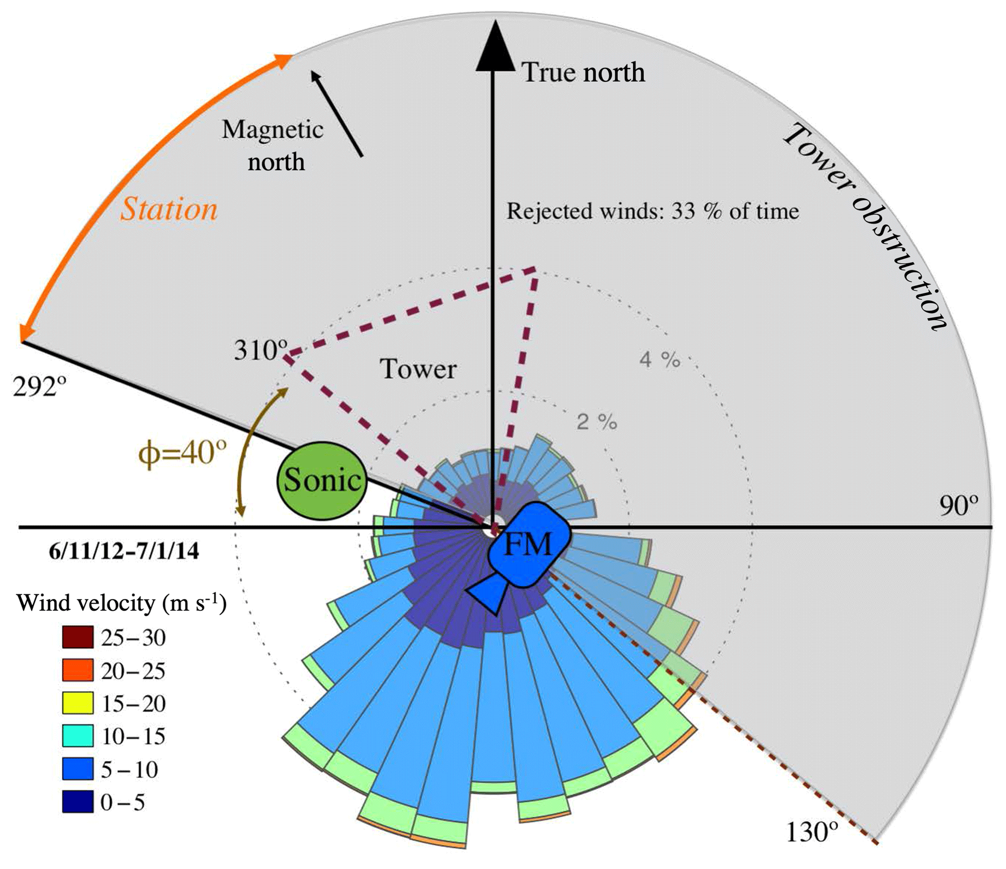
Figure 1Schematic plan view of the field setup of the FM100 (blue icon labeled “FM”) on the tower (dashed triangle) at Summit Station. The green oval (“Sonic”) is the position of the Metek sonic anemometer. The grey shaded area shows the wind directions that were rejected and the orange arrow denotes the sector facing the station. The wind rose is also shown cantered on the FM position.
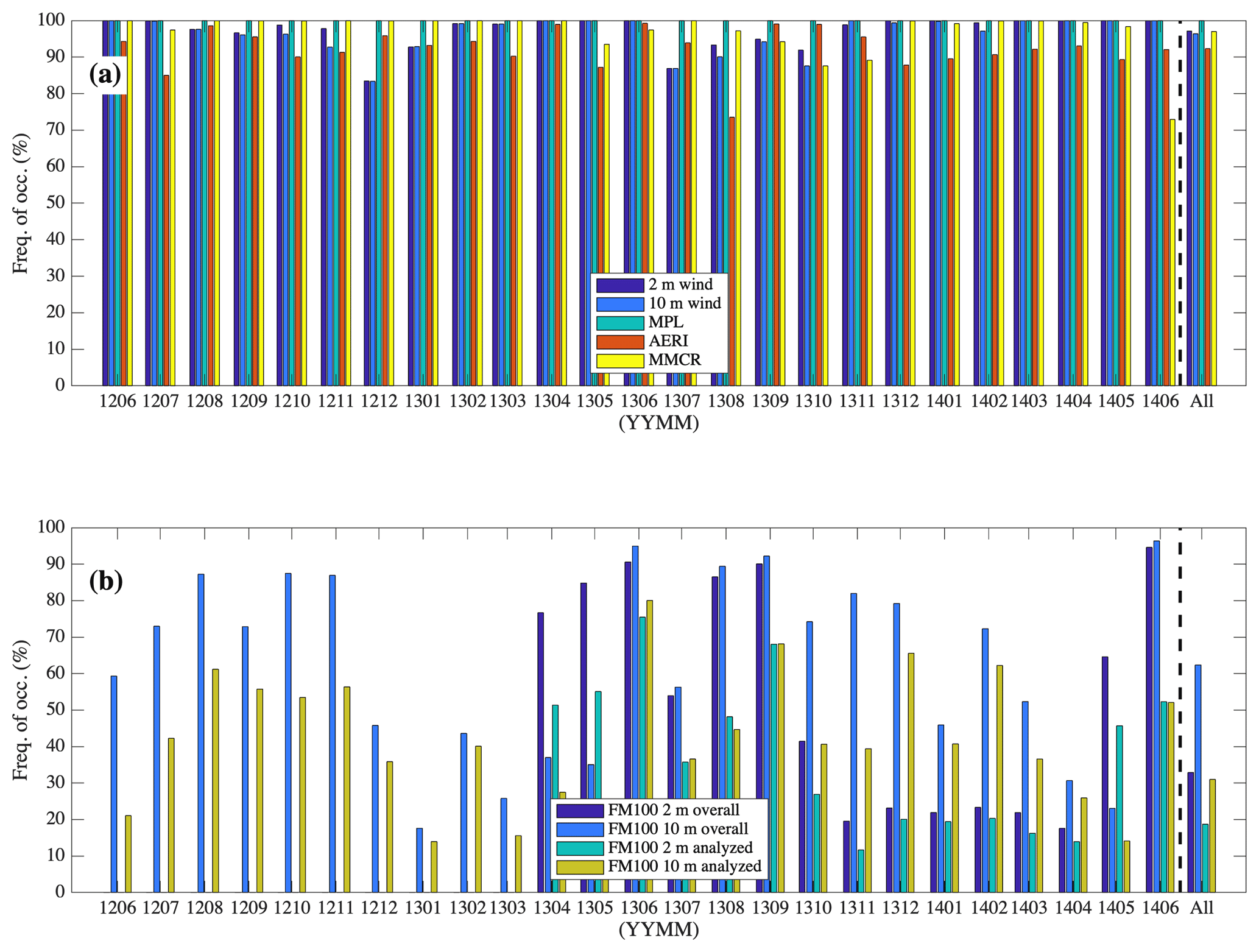
Figure 2(a) Percent of available data: wind (blues), MPL (green), AERI (red), and MMCR (yellow) for each month in the study period. (b) Similar to panel (a) but for the FM100s at 2 m (dark blue and green) and 10 m (light blue and yellow). Blues show the amount of available data while yellow and green show the amount of analyzed data after screening for wind direction and availability of ancillary measurements from panel (a).
Valid observations for each FM100 require availability of all ancillary measurements (Fig. 2a) and also that the wind direction relative to the probe inlet horn was within an acceptable range (refer to the Supplement). For this work, fog microphysics is only presented for data collected when the wind direction was within 50∘ of the inlet horn while radiative, meteorological, and occurrence data are presented for all previously described valid wind directions with respect to the tower. Figure 2b shows both the operational uptime and effective uptime (or microphysical analysis uptime) for the FM100s, given these criteria. The effective uptime varied between about 10 % and 80 %, depending on the month. The 2 m FM100 was not operational until April 2013 due to mechanical problems. In general, uptime was greater than 50 % during the summer but was less than 50 % in winter. Downtime was typically due to data dropouts associated with cold-soaked electronics.
Wind velocity and direction are necessary for processing the data acquired by the FM100s. At Summit, wind measurements were acquired from Metek USA-1 sonic anemometers that were installed alongside both FM100s. These data were acquired at ∼20 Hz and were averaged to 1 min. The anemometers were operated year-round and were heated during icing conditions to prevent riming and frosting of the sensors. Overall, the sonic anemometer at 2 m was operational 74 % of the time and the sonic anemometer at 10 m was operational 79 % of the time during the study period. Gaps in the data at both heights were filled using the station measurements. Though local wind measurements are preferred, this is justified because for wind directions in the range used for analysis, the station data were well correlated with sonic anemometers (at 10 m (2 m) r2=0.94 (0.88) and 0.88 (0.78) for wind speed and direction, respectively). With the station data supplementing the sonic anemometers, the total availability for wind measurements was >99 % for the valid range of wind directions at both heights.
The FM100 is a single-particle light-scattering spectrometer. The instruments were adapted for cold temperatures by limiting internal ventilation of electronics and adding external insulation around the instruments. Ambient air is drawn into a contraction horn inlet using pumps installed on the tower. The air flow within the instrument (the probe air speed, PAS) is measured continuously with a Pitot tube located in the probe's inlet tunnel; at Summit, the PAS was approximately 15 and 7.5 m s−1 at 2 and 10 m, respectively. Sample air in the instrument is drawn past a narrow 658 nm laser. Hydrometeors that pass through the inlet scatter the beam and a portion of the forward-scattered light (between approximately 3 and 12∘) is collected by a detector. An equivalent optical diameter is then derived for each particle from the voltage measured by the detector, which is calibrated to the scattering cross sections for liquid spheres. The detectable particle size range is 1–50 µm and individual detections are binned to provide size distribution measurements at 1 Hz. The data were averaged to 1 min temporal resolution. Thus, for the present work, the term particle size refers to measurements of individual hydrometeors averaged over measurements made 60 times each minute and should be interpreted as an optically equivalent diameter of spheres, regardless of the particle's geometric shape. Refer to Borrmann et al. (2000) for information on sizing errors associated with ice particles.
There are two main uncertainties associated with the FM100 measurement (Spiegel et al., 2012). The first is sizing ambiguities arising from the nonmonotonic Mie scattering function used to convert voltage measured at the detector to particle size. Following Pinnick and Auvermann (1979) and Dye and Baumgardner (1984), ambiguous sizing bins were identified and combined. The second set of uncertainties involve sampling losses in the aspiration and transmission of particles. The data were corrected for these biases following the recommendations of Spiegel et al. (2012). Details of this post-processing can be found in the Supplement.
Between November and March, the FM100 heaters were frequently unable to maintain continuously ice-free Pitot tubes, resulting in disruptions to the monitoring of the PAS. The problem affected the 2 m instrument more because it was located closer to the surface where the temperature is typically colder, and the problem persisted even after insulation was applied to the instrument case. Analysis of the data, in addition to measurements made by station technicians, confirmed that the pumps continued to operate normally during this time. In spring, the return of sunlight was found to provide sufficient heating to correct the problem, even when temperatures remained low. The affected data were recalculated using the mean PAS for normal operating conditions, which varies by approximately ±5 % (1σ). Note that the pumps may operate more efficiently in colder temperatures, potentially producing a small positive bias in estimated PAS.
Several ICECAPS datasets were also used to support the analysis of the probe data, including from an atmospheric emitted radiance interferometer (AERI), a millimeter cloud radar (MMCR), a microwave radiometer (MWR), a micropulse lidar (MPL), radiosondes, and a sodar acoustic sounder. The AERI is a self-calibrated infrared spectrometer (Knuteson et al., 2004a, b) that acquires spectra at subminute intervals from about 490 to 3000 cm−1 (3–20 µm) with a spectral resolution of ∼1 cm−1. The spectra were post-processed using a principal components algorithm that reduces spectral noise (Antonelli et al., 2004; Turner et al., 2006). Quality control procedures removed 7.7 % of the data due to instability of the reference sources, excessive noise, and iced optics (Fig. 2a). The AERI is used to determine the phase of particles measured by the FM100s, as described in Sect. 3. The MMCR and MPL data were used to identify tropospheric clouds. The MMCR is a zenith-pointing 35 GHz Doppler radar (Moran et al., 1998) with high sensitivity to cloud particles and little attenuation through the typical clouds observed at Summit. It samples with ∼4 s temporal and 45 m vertical resolutions. It has been used previously to identify precipitation at Summit by Castellani et al. (2015) and Pettersen et al. (2018). The MPL is a 532 nm depolarization lidar with 5 s temporal and 15 m vertical resolutions. The MPL data product used here is from a phase-resolved cloud mask described by Edwards-Opperman et al. (2018). MWR data are used to retrieve liquid water path (LWP) during fog conditions using a physical retrieval algorithm (Turner et al., 2007). The sodar (Neff et al., 2008) is a 2100 Hz acoustic sounder that samples every ∼1 s with a vertical resolution of 1 m. More details on each of these instruments and data streams can be found in Shupe et al. (2013) and references therein.
Broadband radiometric fluxes (Shupe and Miller, 2016) were measured by Kipp & Zonen CG4 pyrgeometers (longwave) and CM22 pyranometers (shortwave). The processing of these data is described by Miller et al. (2015, 2017). Cloud radiative forcing (CRF) is defined as the instantaneous effect of clouds on the radiative flux at the surface. CRF is calculated by subtracting a modeled clear-sky estimate from the measured radiative flux, as described by Miller et al. (2015). The cloud radiative effect of the longwave component (LWCRE) is calculated in the same manner as CRF but only includes measured and modeled estimates from the downwelling longwave component (e.g., Cox et al., 2015). Sensible and latent heat fluxes (Shupe and Miller, 2016) were estimated via the bulk aerodynamic method and a two-level approach (10 and 2 m), respectively (Miller et al., 2017).
3.1 Introduction to the classification
The FM100 observations may be liquid fog, ice fog (note that we do not distinguish between ice fog and clear-sky precipitation, also known as “diamond dust”), blowing snow, or snow. Thus, it is desirable to classify the probe observations in order to identify the scenes containing liquid fogs. To do this, information about particle phase, precipitation occurrence, the presence of elevated cloud layers, and the likelihood of blowing snow is needed.
The classification procedure is as follows: (1) scenes containing near-surface particles are separated from clear boundary layer scenes using a number concentration (Nc, cm−3) threshold in the 10 m FM100, (2) elevated tropospheric cloud layers are identified, followed by (3) occurrences of blowing snow and snow, and then (4) the phase of the particles is determined for all cases where particles were observed near the surface (step 1) but the sky was otherwise clear (step 2) and there was no blowing snow (step 3). Next, we will describe the individual classifications.
3.2 Classification steps
3.2.1 Identification of near-surface particles
A large proportion of the observations at Summit are of particle concentrations with low density (<1 cm−3), such as snow and light blowing snow. It is desirable to set a threshold low enough to capture these conditions. Using an FM100, Spiegel et al. (2012) set a threshold Nc>10 cm−3 for similar purposes, which is low enough to observe snow (Braham, 1990). Figure 3 shows frequency of occurrence of FM100 observations classified as containing any type of surface-based cloud (red and black lines) as a function of Nc. The other lines in the figure represent classifications of cloud types that are discussed later. Overall, particles are identified ∼80 % of the time at 10 m when the threshold for detection is 10−3 cm−3. Due to the consistent volume size of the FM100, this is also roughly the lowest Nc it can measure. Therefore, cm−3 is a natural threshold for this study.
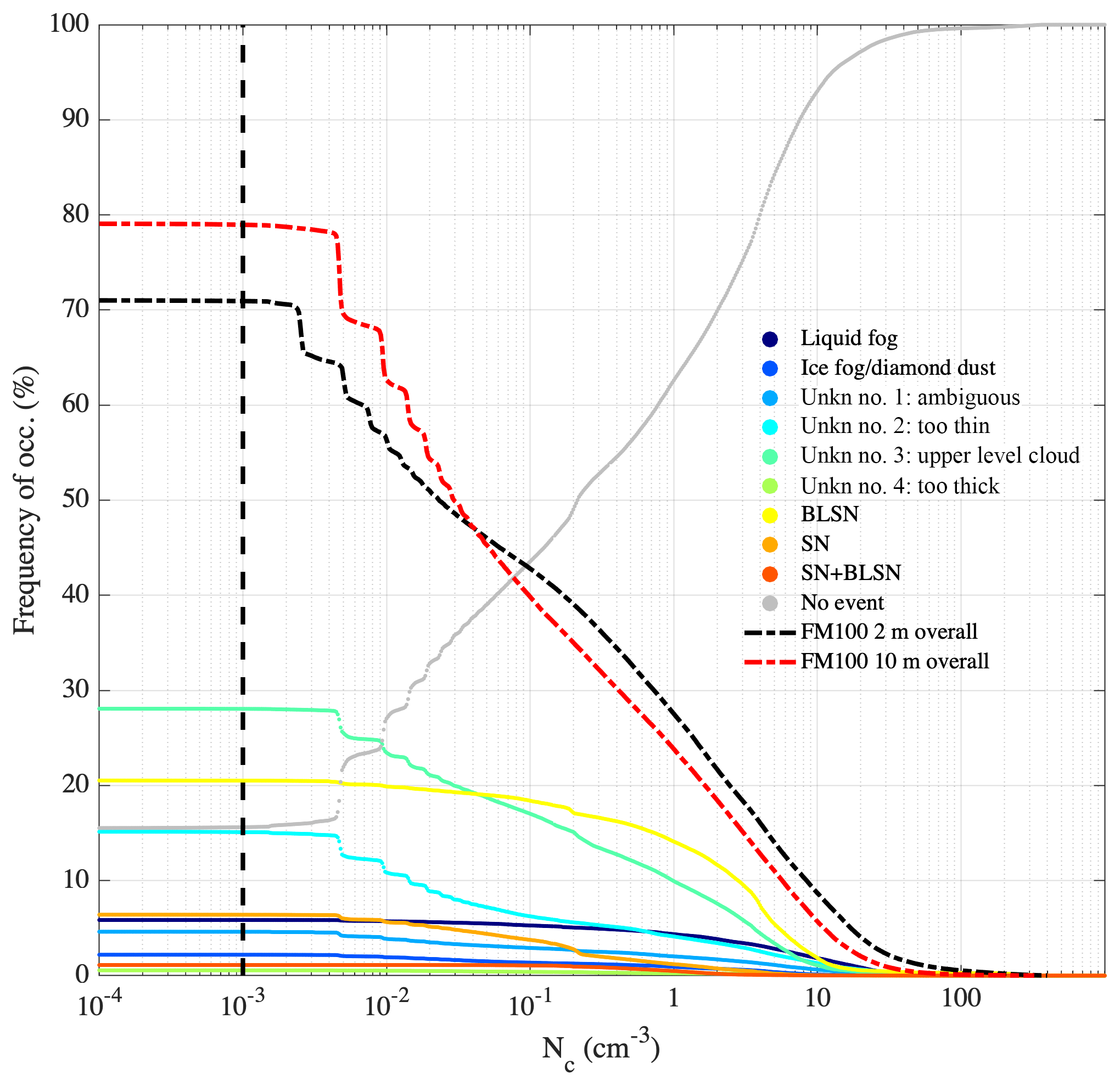
Figure 3Percent of time clouds are identified in FM100 data at 2 m (black dashed) and 10 m (red dashed) as a function of threshold in number concentration. Colors show the same for the classifications that are reported in Fig. 5.
3.2.2 Tropospheric clouds
Scenes with elevated cloud layers are identified because the phase classification (see below) is only valid when no other clouds are present in the scene. Cases with elevated cloud layers are therefore rejected from analysis of the fogs presented later. Using the MPL cloud mask, elevated clouds are defined as clouds with bases above 200 m, similar to the definitions used by Starkweather (2004) and Castellani et al. (2015).
3.2.3 Snow and blowing snow
Radar reflectivities greater than −5 dBZ, which are indicative of light snow (Shupe et al., 2013), are used as a conservative threshold to identify precipitation falling between 200 and 300 m. These particles are assumed to be formed above the height of blowing snow and fall to the surface as precipitation and are therefore classified as snow. While estimates of the depth of blowing snow layers are currently unavailable at Summit, layer depths exceeding 300 m are infrequent in Antarctica and when they do occur they generally coincide with precipitation (Gossart et al., 2017). The radar data are combined with wind parameterizations for lofting (i.e., blowing) snow calculated for western Canada by Li and Pomeroy (1997). When the radar data indicate snow and the Li and Pomeroy parameterization indicates blowing snow, the classification of a combination of snow and blowing snow is assigned.
3.2.4 Phase classification
Events composed of ice are distinguished from those composed of liquid using the AERI data, which are collected at intervals of about 20–75 s. These spectra are linearly interpolated to the regular 1 min sampling used for the FM100 data. The imaginary component of the complex index of refraction, which is proportional to absorption, has different spectral dependencies for ice and liquid in the infrared. Previous studies have exploited these dependencies to infer particle phase using spectral differencing techniques (Strabala et al., 1994; Turner et al., 2003). Particle size and habit also exhibit spectral dependencies, which are a large source of uncertainty in these methods, as is uncertainty in water vapor amount and cloud temperature. In general, the uncertainty also increases for optically thin clouds because of reduced signal and for optically thick clouds because of loss of spectral structure (Turner, 2005). However, the spectral differencing approach is justified for this work because the cases of interest are less sensitive to the associated uncertainties. First, atmospheric transmission between the surface and the cloud is close to unity in the dry Arctic atmosphere (Turner et al., 2003) and can be assumed to be unity for the present purposes because the focus is on clouds with bases at the surface. Second, cloud temperature is well-characterized because it is measured in situ. Finally, because the scenes that are tested feature fogs that were observed when the sky was otherwise clear, it is reasonable to assume that these scenes were single-layer, negating ambiguity from multiple cloud layers.
Calculations of cloud emissivity are used for the phase identification using spectral microwindows that are sensitive to cloud detection (Turner et al., 2003). The necessary radiative transfer calculations were performed using the Line-by-line Radiative Transfer Model (LBLRTM), version 12.2 (Clough et al., 2005). Inputs to LBLRTM include twice daily radiosonde profiles from Summit and estimates of trace-gas profiles, as described by Cox et al. (2014). A small positive bias common in AERIs (less 0.5 mW m−2 sr−1 (cm−1)−1) was estimated empirically for each microwindow by comparison to the radiative transfer calculations during clear days and was subtracted from the microwindow radiance before analysis.
We use two spectral cloud emissivity differencing tests. The first, adapted from Strabala et al. (1994), is a threshold set to the 11 minus 12 µm emissivity versus the 11 minus 8.1 µm emissivity. The threshold to separate the clusters was qualitatively set to . As indicated by the example in Fig. 4a, the clusters separate distinctly and therefore the precise slope of the threshold is not important. The second test is applied in the far-infrared spectral region where ice and liquid absorption characteristics are different and determines whether the 11 minus 17.8 µm emissivity is greater or less than zero (see example in Fig. 4b). If both tests agree, the identification is deemed valid. If the tests disagree, the observation is considered ambiguous. Ambiguous identifications are expected when the microwindow differences are near zero, which typically occurs when the emissivity of the fog is low. However, Fig. 4b also indicates that a small number of cases are not clustered as expected in the far-infrared region, even when the microwindow signal differences are large (red points near the center of the figure). The reason for these ambiguous identifications is not known and their source may be from instrumental errors or environmental conditions. These cases represent <1 % of the data, and the methodology has successfully screened them out.
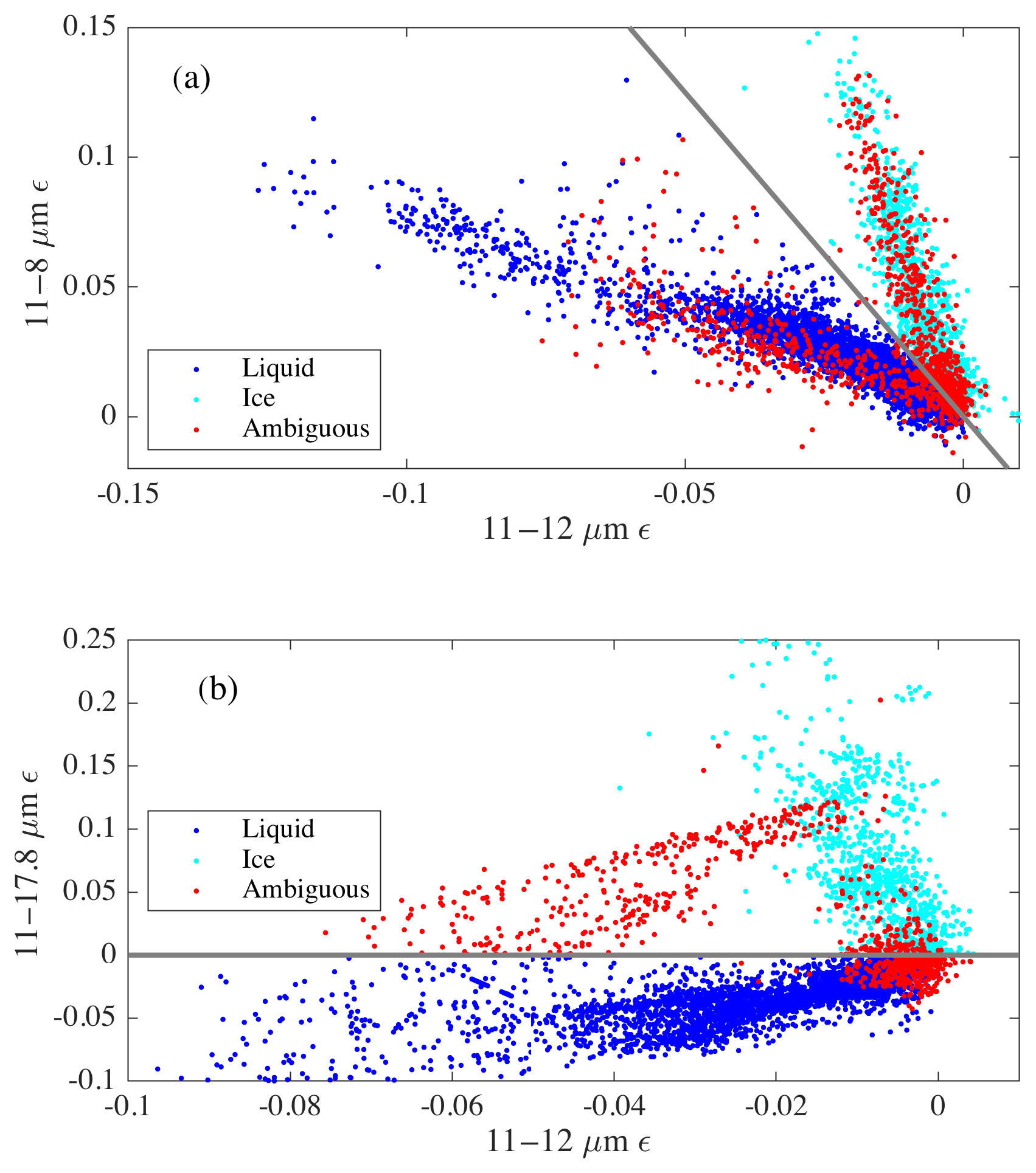
Figure 4Example of phase classification using microwindow cloud emissivity measured by the AERI for the month of June. Panel (a) shows the first test described in the text and panel (b) shows the second. The colors indicate the classification. Only scenes containing identified events where the AERI 11 µm emissivity was >0.02 and no upper-level clouds were detected are shown (n=4527).
3.3 Summary of classification
Figure 5 summarizes the fractional occurrence of the classified cloud types. Particles were observed in the lowest 10 m for a majority of the time in all months, from 65 % of the time in July to >85 % of the time in winter. Liquid fogs under otherwise clear skies were classified between 1 % of the time (April) and 12 % of the time (September); if liquid fogs could be reliably detected in the presence of tropospheric clouds, these percentages would likely be higher. While most common in late summer, liquid fogs were also identifiable 3 %–7 % of the time during January–March. The fact that there were fewer ice identifications than liquid identifications does not necessarily indicate that in situ formation of ice near the surface at Summit is less common than liquid formation for three reasons: (1) the number density of liquid fog is expected to be higher, so liquid is more likely to be identifiable using the AERI, (2) some ice fog events may be incorporated within the blowing snow or snow categories, and (3) the phase partitioning for events from which phase could not be retrieved using the AERI is unknown.

Figure 5Composite monthly frequencies of occurrence of each classification. BLSN and SN refer to blowing snow and snow, respectively. Precipitation occurrence is the sum of SN and BLSN+SN.
The classification scheme reveals several key features of hydrometeor occurrence over the Greenland Ice Sheet:
-
Precipitation occurred predominantly from July through to October (similar to the study by Pettersen et al., 2018). This seasonal cycle is shifted later in the year compared to total precipitation amount, which peaks in July (Castellani et al., 2015).
-
In months when blowing snow occurred most frequently (winter and spring), precipitating snow was less common; and during summer when most of the precipitating snow occurred, blowing snow was least common.
-
A high frequency of events (composite annual average =27.3 %) was detected by the 10 m FM100 under tropospheric clouds, which are common at Summit (Miller et al., 2015).
-
Identification of ice fog was less frequent than liquid fog and ice fog had a distinctly different seasonal cycle than that of liquid, with a peak in April (9.2 %) and a low in July (0.3 %).
We contrast two cases of liquid fogs to illustrate the conditions captured with the categorization scheme. We first discuss a case of near-idealized fog formation conditions that appeared on the 16 June 2013 in Sect. 4.1. Then, this case is contrasted with a winter case from January 2014 in Sect. 4.2. The discussion of the time evolution of the fogs assumes spatial homogeneity. While the meteorology observed during the cases generally supports this assumption, we cannot rule out advection, either from distant regions or associated with local topographical variability (–3 m) as a source of some of the observed variability.
4.1 Case of 16 June 2013
Clear skies persisted from 15 to 24 June 2013, and liquid fogs were observed in the early morning on most days during this period. While this case represents an ideal illustration of fog formation at Summit, several similar cases can be found in the dataset. Figure 6a and b show the time–particle-size cross sections of Nc from the FM100s beginning at 20:00 UTC on 15 June extending through 14:00 UTC on the 16 June. During this period, the 10 m air temperature was −15 to −22 ∘C with light southerly winds (Fig. 6e). At 10 m, condensate first occurred ∼00:10 UTC as the solar elevation angle (SEA) dipped to 10∘ (<20 W m−2 SWnet, Fig. 6d) and 7 h into development of the surface-based inversion (Fig. 6d). Initiation was followed by a period of uniform growth lasting 4–5 h that closely aligns with a theoretical growth curve (Houghton, 1985), calculated assuming a constant supersaturation of 0.1 % (Fig. 6a). During the first hour of growth, the droplets reached approximately 25 µm in diameter after which the growth slowed and deviated from the theoretical curve, with particles eventually reaching ∼40 µm. The curve neglects the gradual decrease in supersaturation that accompanies condensation without replacement of moisture, implying a decrease in supersaturation during development and indicating that the moisture source did not introduce new vapor as quickly as it was condensed. While most of the droplets closely followed the main growth curve, nucleation of new droplets continued until about 03:00 UTC. The fog disappeared completely by ∼10:30 UTC when the sun reached an elevation angle of ∼30∘.
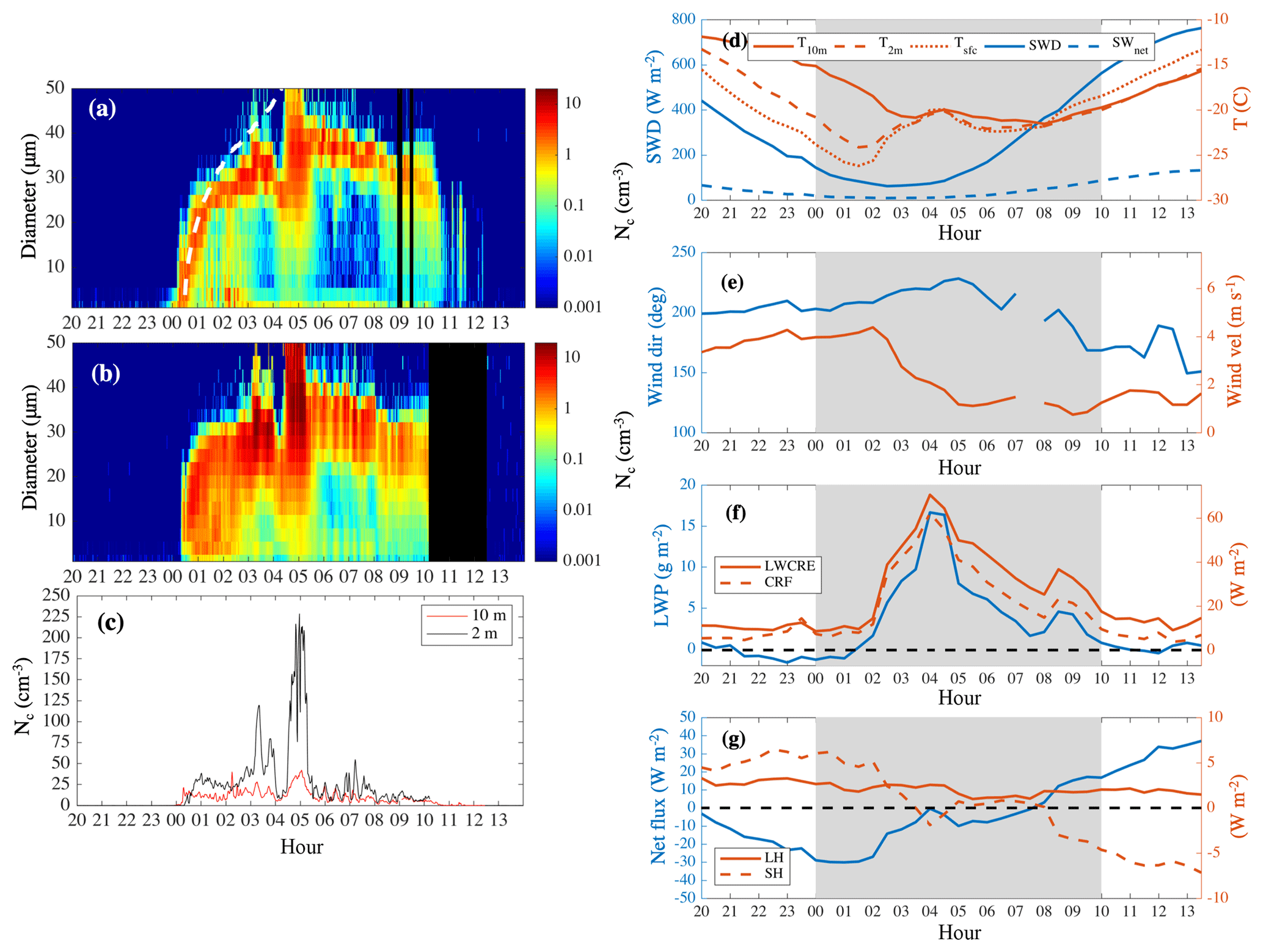
Figure 616 June 2013 case study. Number concentration and particle diameter from FM100 at (a) 10 m and (b) 2 m. (c) Total number concentration (Nc) in all bins for the 10 m FM100 (red) and the 2 m FM100 (black). (d) Temperatures at surface (skin), 2 and 10 m (reds) and downwelling shortwave radiation (SWD) and net shortwave radiation (SWnet) (blues). (e) Wind direction (blue) and velocity (red). (f) Longwave cloud radiative effect (LWCRE) and total cloud radiative forcing (CRF) (reds) and liquid water path (LWP) (blue). (g) Latent (LH) and sensible (SH) (reds) turbulent fluxes and net flux (blue). The white dashed line in panel (a) is a theoretical growth curve calculated from Houghton (1985).
The sodar detects thermal turbulence where mixing occurs within a vertical temperature gradient. Note that structure in the sodar record may only reflect structure in temperature and not necessarily the boundaries of the fog; although in some cases radiative cooling at the top of the fog may account for the thermal contrast that is observable with the sodar. The sodar record shows a typical pattern of a “nighttime” stable surface layer 10–25 m deep before 07:00 and after 20:00 UTC (Fig. 7a). This surface layer represents a shallow, but strong, temperature inversion embedded within a deeper inversion that extended about 100 m above the surface at initiation, further deepening to several hundred meters 12 h later. The surface layer increased in depth from about 15 to about 65 m during the course of the duration of the fog layer, transitioning from statically stable to a shallow convective layer in association with the diurnal cycle (Fig. 7a). The convective plumes are visible in Fig. 7a as vertically oriented echoes below the red dashed line with intervals on the order of minutes. Dissipation occurred shortly after the onset of convection ∼08:45 UTC (SEA ∼23∘, SWnet=61 W m−2, SWD =426 W m−2), and the fog disappeared when the convection reached a developed stage around 10:00 UTC (SEA ∼29∘, SWnet=87 W m−2, SWD =562 W m−2).
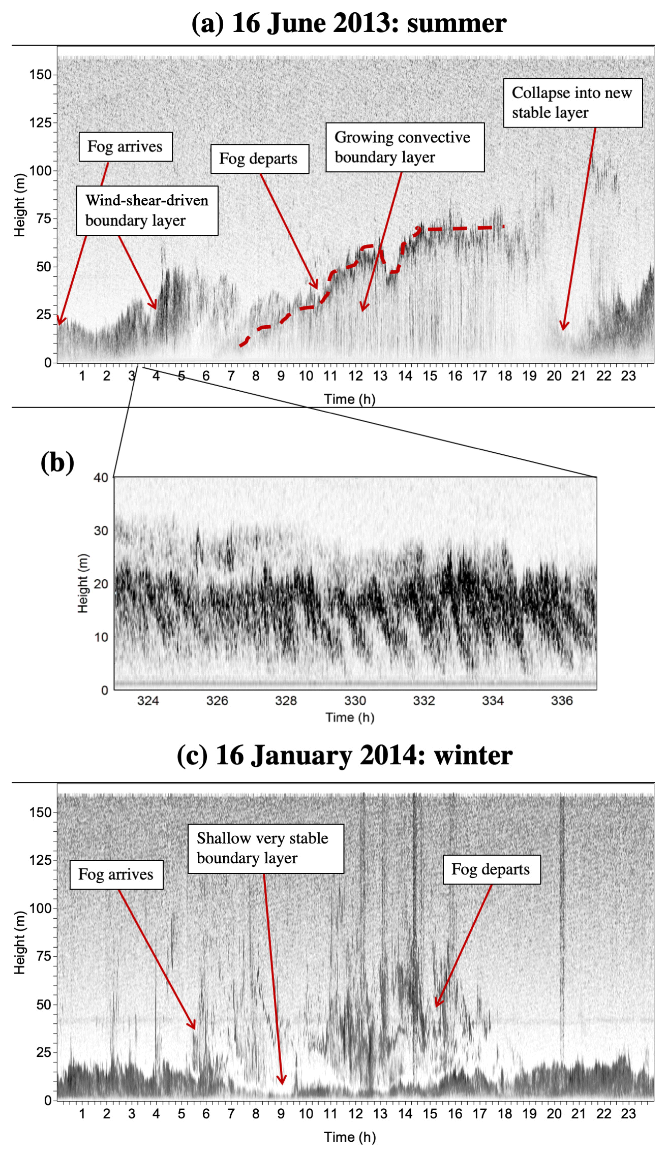
Figure 7Sodar facsimile records between the surface and 160 m height for the summer case (16 June 2013, a). Panel (b) shows an expansion of a brief period from 03:23 to 03:37 UTC and 0–40 m height from panel (a) to highlight the Kelvin–Helmholtz instabilities observed at this time. Panel (c) is similar to (a) but for the winter case on 16 January 2014. Dark features that extend to the top of the plot in panel (c) (e.g., near 20:00 UTC) are likely noise from station activities and the horizontal feature in panel (c) near 40 m height is due to reflections of a side lobe from an object nearby on the ice surface.
Particles were observed at 2 m 10–20 min after initiation at 10 m. Both the Nc and the width of the size distribution were larger at 2 m than 10 m, consistent with particle formation near 10 m followed by settling and evaporation (∼ 0.01 m s−1). At Summit, condensation in radiation-induced fog frequently occurs near 10 m because nonlinearity between temperature and saturation within the inversion leads to supersaturation first between 3 and 18 m, with lower vapor pressures both above and below this layer (Berkelhammer et al., 2016). A lag in Nc of 3 to 4 min between 10 and 2 m near the peak particle size is evident in the time series (Fig. 6c), implying a maximum settling rate of 0.03 to 0.04 m s−1. Theoretical calculations of settling rates assuming laminar conditions following Pruppacher and Klett (2010) agree with these estimates. Specifically, the calculations indicate settling rates up to 0.01 m s−1 during the first hour of the case and 0.03–0.035 m s−1 during the mature phase of the fog between 06:00 and 08:00 UTC.
Between 02:00 and 05:00 UTC, the 2 m air temperature deviated by ∘C from the smooth diurnal cycle that is evident both before and after the fog, and the LWP increased to ∼15 g m−2 with no clouds observed above the fog layer by the radar or lidar. This corresponded to an increase in CRF from <10 to ∼65 W m−2, caused primarily by increased downwelling longwave radiation, as evidenced by the LWCRE (Fig. 6f). These values are within the range of the thickest clouds at Summit (Cox et al., 2014; Miller et al., 2015) and large enough to drive latent and sensible heat fluxes to near-neutral conditions (Fig. 6g), indicating a well-mixed surface layer. As we will see later, fogs generally produce closer to ∼10–20 W m−2, but larger values such as the 16 June case occur occasionally. Because of these factors, the temperature inversion within the surface layer completely eroded by around 03:30 UTC. Surprisingly, this did not dissipate the fog, and, in fact, an increase in Nc at 2 m occurred in conjunction with a brief interruption in the otherwise smooth growth rate. Following the brief interruption, the particle size and Nc were larger than before with Nc at 2 m exceeding 200 cm−3; as we will see later, such high Nc as observed from 04:00 to 05:00 UTC are atypical.
Thus, while the fog was likely induced by radiation initially, it was maintained, and ultimately continued to grow, without additional infrared loss at the surface driving saturation in the air column. Indeed, with warming of the surface layer, introduction of large quantities of vapor would have been necessary to maintain the relative humidity supporting the fog. The large LWP (Fig. 6f) implies significant cloud-top radiative cooling may have occurred; therefore, buoyancy-driven mixing is a plausible mechanism to have supplied the moisture that maintained the fog. However, the moisture was more likely introduced to the surface layer from above by mixing generated by wind shear. This is supported by the sodar data, which shows signatures of turbulence in the form of Kelvin–Helmholtz instabilities (Fig. 7b) driven by shear at the top if the surface layer (30–50 m) between 03:00 and 05:00 UTC, corresponding to the period of time with enhanced LWP, CRF, and Nc, and generally more variable particle size at both measurement heights. Indeed, in June, the firn is generally colder than the surface (Miller et al., 2017) so vapor transfer tends to be downward, toward the surface, from the atmosphere because the mixing ratio is higher in the (saturated) air immediately above the surface than in the firn (Berkelhammer et al., 2016). The latent heat flux (LH) was positive (defined positive into the surface) for the duration of the case study, consistent with the hypothesis that the fog was driven by moisture from aloft (Fig. 6g). Therefore, the moisture source for this case was likely the atmosphere and not the local surface. Interestingly, the Nc at 10 m was consistently lower than at 2 m. The reasons for this are unclear but since there were also more small particles at 2 m, it is possible that the concentration of particles at 2 m was associated with partial evaporation and subsequent slowing of the particles descent. The difference may also be associated with the heights of the instruments relative to the height of maximum supersaturation (see Fig. 2 by Berkelhammer et al., 2016).

Figure 816 January 2014 case study. Number concentration from FM100 at 10 m (a) and 2 m (b). (c) Total number concentration (Nc) in all bins for the 10 m FM100 (red) and the 2 m FM100 (black). (d) Cloud mask from the MPL: yellow is ice, green is liquid, blue is clear, and black is below the minimum height for acceptable data. The height scale is log. (e) Temperatures at surface (skin), 2 and 10 m (reds), and downwelling shortwave radiation (SWD), net shortwave radiation (SWnet), and solar zenith angle (minus 93 then divided by 10 to fit on the figure) (blues); (f) wind direction (blue) and velocity (red); (g) longwave cloud radiative effect (LWCRE) and total cloud radiative forcing (CRF) (reds) and liquid water path (LWP) (blue). (h) Latent (LH) and sensible (SH) (reds) turbulent fluxes and net flux (blue).
4.2 Case of 16 January 2014
Figure 8 is similar to Fig. 6, but for a wintertime case. The fog was detected at ∼05:30 UTC at 10 m, and the particles grew quickly to ∼35 µm within approximately 30 min (Fig. 8a, b). The Nc at both heights was about an order of magnitude smaller than the June case (Fig. 8c). The troposphere was clear with intermittent ice clouds above 2 km (Fig. 8d). Similar to the June case, the wind was southerly and light with lower wind speeds during the period of the fog (Fig. 8f). The net atmospheric heat flux was generally negative (Fig. 8h) due to radiative cooling at the surface that maintained a temperature inversion with a gradient of ∼10 ∘C between 2 and 10 m (Fig. 8e). There was not enough LWP for reliable detection by the MWR (uncertainty ∼5.5 g m−2), but the CRF was between 10 and 40 W m−2; note that the upper-level clouds contributed some to this forcing, in particular after 14:30 UTC. The CRF quickly spiked to 40 W m−2 during the initial fog development around 06:00 UTC, which was also the time period when the Nc was the highest. Later increases in CRF also corresponded in time to increased Nc. Consistent with variable wind direction, the apparent intermittence of Nc may be explained by a spatially heterogeneous fog periodically passing the tower instruments.
This case was likely a mixed-phase fog with a liquid formation layer precipitating into an underlying settling layer composed of homogeneously frozen ice. The air temperature at 10 m (near the formation height) was between −35 and −38 ∘C. While the homogeneous freezing point for liquid is imprecise and dependent on conditions (generally about −40 ∘C), the 2 m air temperature and skin temperatures were and −50 ∘C, respectively, both too cold to support liquid particles. Thus, it is likely that the particles observed at 2 m were frozen droplets. While we can only infer the phase of the underlying layer from the measured temperature, we do have confidence that the droplets that formed aloft were liquid: the AERI classifications were not ambiguous as 176 of 177 samples for this event were identified as liquid; the AERI classification should not have been confounded by the presence of the ice because the viewport for the AERI is a few meters above the surface, and therefore near the top or above the ice layer; the AERI results are also supported by the MPL data, which indicate mostly liquid at levels where the MPL has sensitivity, between 100 and 150 m (Fig. 8d).
The ceilometer (not shown) and MPL (Fig. 8d) data indicate a deeper fog layer than the previous case, which may have been enabled by generally deeper and more persistent inversions in winter (Miller et al., 2013); the height of the maximum temperature within the troposphere for this case was 300–400 m compared to ∼100 m at initiation for the June case. However, the sodar record (Fig. 7b) shows that the depth of the surface layer embedded within the deeper inversion for the winter case was actually much shallower than in the summer case, <10 m during the duration of the fog. The particles within the surface layer were sampled by the measurements made at the tower (e.g., Fig. 8a, b) and may be distinct from the deeper fog layer visible in the MPL data: the sodar record also shows a significant amount of structure throughout the upper fog layer indicating additional stable layers (Fig. 7c). This structure is physically decoupled from the surface layer, separated by a thin layer of low reflectivity that may be indicative of a low-level jet, which could suppress mixing between the layers. However, the layers may be dynamically coupled in other ways. Buoyancy waves with periods of a few minutes to 15 min in the upper layer have an observable remote influence on the surface layer through fluctuations in the horizontal pressure field that produce a moving pattern of convergence and divergence (not shown). It is unknown if the observed microphysics below 10 m is representative of the fog above the surface layer. However, radiatively, the combined physically thick layer of fog compensates somewhat for the low Nc observed near the surface, enhancing the CRF relative to the summer case with a larger optical depth. The strength of the inversion also contributed to enhancing the CRF because the particles were warmer than the surface.
Interestingly, the fog development coincides closely with the weak early-season diurnal cycle. In mid-January, the sun does not rise above the horizon at Summit but is about 3∘ below the horizon at solar noon (Fig. 8e). Atmospheric scattering in these twilight conditions produced 1–3 W m−2 of diffuse incident solar radiation (Fig. 8e) that corresponded in time with the fog initiation. Though the mechanism is unknown, there is a possibility that the fog was diurnally forced, similar to the June case; yet, unlike summer, the timing was coincident with a peak in solar radiation rather than the minimum.
The stably stratified surface layer was largely isolated from the free troposphere in this case. The temperature gradient within the firn (which is warmer at depth than at the surface) produces a constant supply of vapor towards the surface from below, providing moisture for the fog, which is then returned via settling (Berkelhammer et al., 2016). As before, we observed higher concentrations and more small particles at 2 than 10 m.
5.1 Physical properties
Figure 9 shows distributions of the particle sizes for liquid fogs (blue) compared to those for the ice categories; the figure displays sensor height as rows (10 m – top row, 2 m – bottom row) and season as columns (left column – low-light winter season, NDJF, and right column – sunlit summer season, JJAS). Ice particles are nonspherical and, thus, the distributions represent an effective size with reference to the scattering properties of spherical liquid; asphericity and orientation are important factors in the sizing of ice using a scattering spectrometer that imposes significant uncertainties (Borrmann et al., 2000). Thus, the distributions of ice classes should be treated cautiously and are shown here for context. The liquid classification stands out distinctly from the ice both in the shape of the distribution and the overall Nc within each size bin. For smaller particles, liquid particles are present in higher concentrations than ice particles in summer and are smaller in winter, while the opposite is generally true for larger particles. Despite the uncertainties in sizing ice particles, the relative Nc within each size bin separates logically between the different types. For example, there are more particles in blowing snow at 2 m than at 10 m, while the two heights show similar concentrations of ice fog. Also, the occurrences of snow have consistently low Nc.
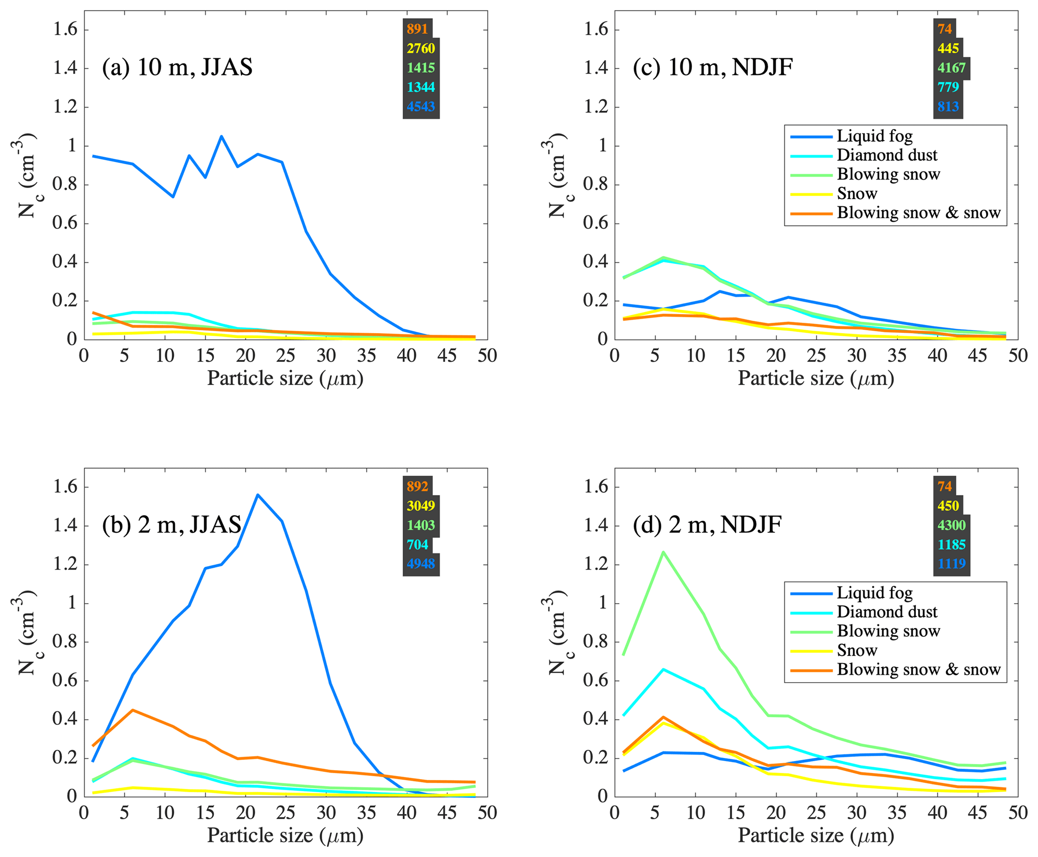
Figure 9Average number concentration (Nc) within the FM100 size bins for different classifications measured at 10 m (top row; a, c) and 2 m (bottom row; b, d). The left column (a, b) is for June–September (JJAS) and the right column (c, d) is for November–February (NDJF). The bin centers for the sizes are 1, 6, 11, 13, 15, 17, 19, 21.5, 24.5, 27.5, 30.5, 33.5, 36.5, 39.5, 42.5, 45.5, and 48.5 µm (refer also to the Supplement for additional information on FM100 sizing). Because the FM100 bin sizes are variable, the bin counts have been normalized such that the integral of the curves equals average concentration for all bins. The values over the grey background are the number of 1 min samples in each distribution.
As implied by the case studies, fogs in winter have lower Nc overall compared to summer. This relationship between temperature and fog Nc is evident when analyzed directly: Nc is smaller in colder fogs, with temperature being correlated with the log of Nc (r=0.54). Gultepe et al. (2002) and Gultepe and Isaac (2004) reported similar findings in tropospheric Arctic clouds containing supercooled liquid. Note that while aerosol concentration is likely a factor, dynamical and thermodynamical processes can also play a role (Gultepe et al., 2002; Gultepe and Isaac, 2004).
The distribution of liquid particles in summer peaks between 20 and 25 µm in diameter at 2 m (Fig. 9b) while the distribution at 10 m (Fig. 9a) is broader with more small particle sizes. This is consistent with particles preferentially forming near 10 m before settling to 2 m. Specifically, multiple growth stages are likely represented in the distribution at 10 m, while the distribution at 2 m is more idealized because it is composed primarily of mature particles. Though the winter liquid distributions are more difficult to interpret owing to a limited number of data, this finding is supported by a calculation of the effective diameter (the ratio of the third and second moments of the size distribution) for all liquid fog scenes in all months, which shows a correlative relationship between effective diameter and Nc at 10 m (Fig. 10a) (), but not at 2 m (Fig. 10b). This indicates that at 10 m, when the Nc is high, the particles are small (forming), while at the same time low Nc for large particles is consistent with loss via settling out of the layer. While a similar relationship might be expected from a range of aerosol concentrations, if aerosols were the explanation for the observations at 10 m, a similar result should be found at 2 m, but it is not.
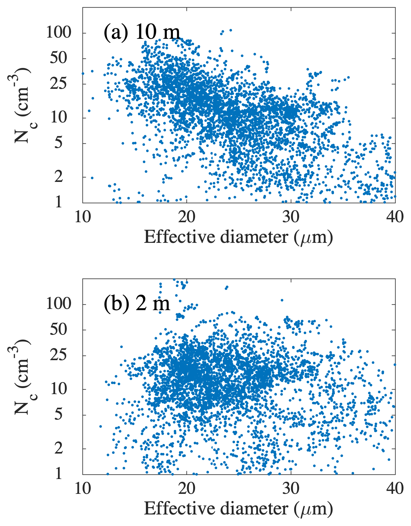
Figure 10Number concentration (Nc) as a function of particle size for liquid fogs measured by FM100s at 10 m (a) and 2 m (b). Note that the y axis is log.
The overall distributions of Nc (Fig. 11) at both heights show concentrations in winter that are smaller than in summer. In winter, there are typically more particles at 2 m than 10 m, whereas during summer the differences between the heights are less discernible. The median value of Nc was typically <7 cm−3 in winter and between 5 and 20 cm−3 in summer (Fig. 11).
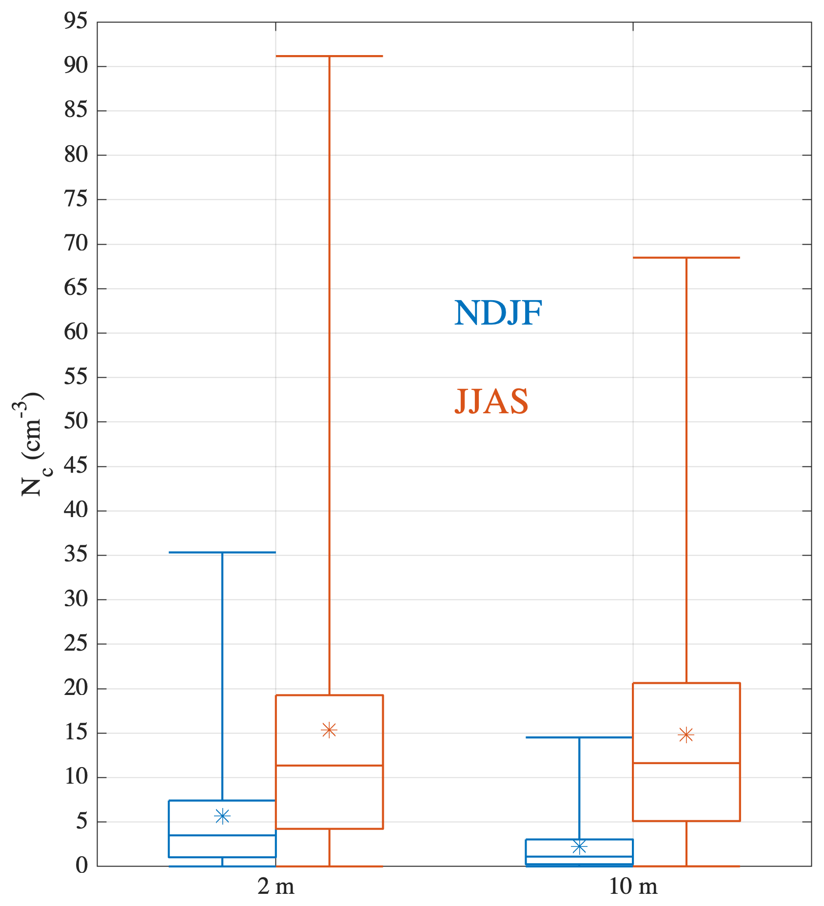
Figure 11Box and whisker plots ( mean, boxes are 25th, 50th, and 75th percentiles, whiskers are 1st and 99th percentiles) for all observations at times when both probes were operational in winter (NDJF, blue) and summer (JJAS, red) at 2 and 10 m.
Figure 12 shows the temperature distributions for times classified as liquid fog and ice fog (the two types associated with in situ formation). In Fig. 12, Nc was only used for identification of events. Thus, precise estimates of Nc are not important, and the threshold for wind direction is less restrictive than the microphysical results shown in Figs. 9–11. Consequently, larger sample sizes are incorporated into this analysis. Three different temperatures are plotted beginning with brightness temperatures derived from near-saturated CO2 emission between 675–680 cm−1 measured by the AERI in Fig. 12a. These frequencies are sensitive to the lowest few tens of meters above the instrument and may be most similar to the fog thermodynamic temperature. Since liquid freezes homogeneously near −40 ∘C, observations at lower temperatures are not possible; less than 1 % of observations classified as liquid occur at temperatures ∘C in Fig. 12a. The air temperatures at 10 m (Fig. 12b) are similar to the AERI-derived temperatures. Air temperatures closer to the surface at 2 m (Fig. 12c) are generally colder and include many more instances with temperatures below −40 ∘C. Note that this is not an indication of water existing in a liquid phase below −40 ∘C but rather indicates that the liquid layer lies above this cold air where the temperature is warm enough to permit the existence of liquid droplets. Between November and March, two-thirds of the liquid fog identifications occurred when the 2 m air temperature was below −40 ∘C. This result indicates that the 16 January case is typical. A stretch of such occurrences was observed when the 2 m air temperature was ∘C during an extended clear-sky period during the last 2 weeks of March 2013. Unlike the 16 January case, for cases during the spring and autumn, there was sufficient daylight for images acquired by cameras mounted to the tower to show evidence of optical phenomena caused by liquid droplets. Images of fogbows appeared at times that coincided with the identification of liquid fogs in March 2013. Fogbows are formed by scattering processes dominated by diffraction when the size of spherical particles is within the Mie regime (e.g., Lynch and Schwartz, 1991). Note that the presence of a fogbow is suggestive of the presence of liquid, but it does not rule out the presence of ice. Additionally, spherical or quasi-spherical ice formed by freezing of supercooled liquid has been reported by other studies (e.g., Thuman and Robinson, 1954), though the preferred habits of ice fog particles remain controversial (see Gultepe et al., 2015) and we are unaware of any studies linking ice fogs to optical phenomena normally associated with liquid droplets.
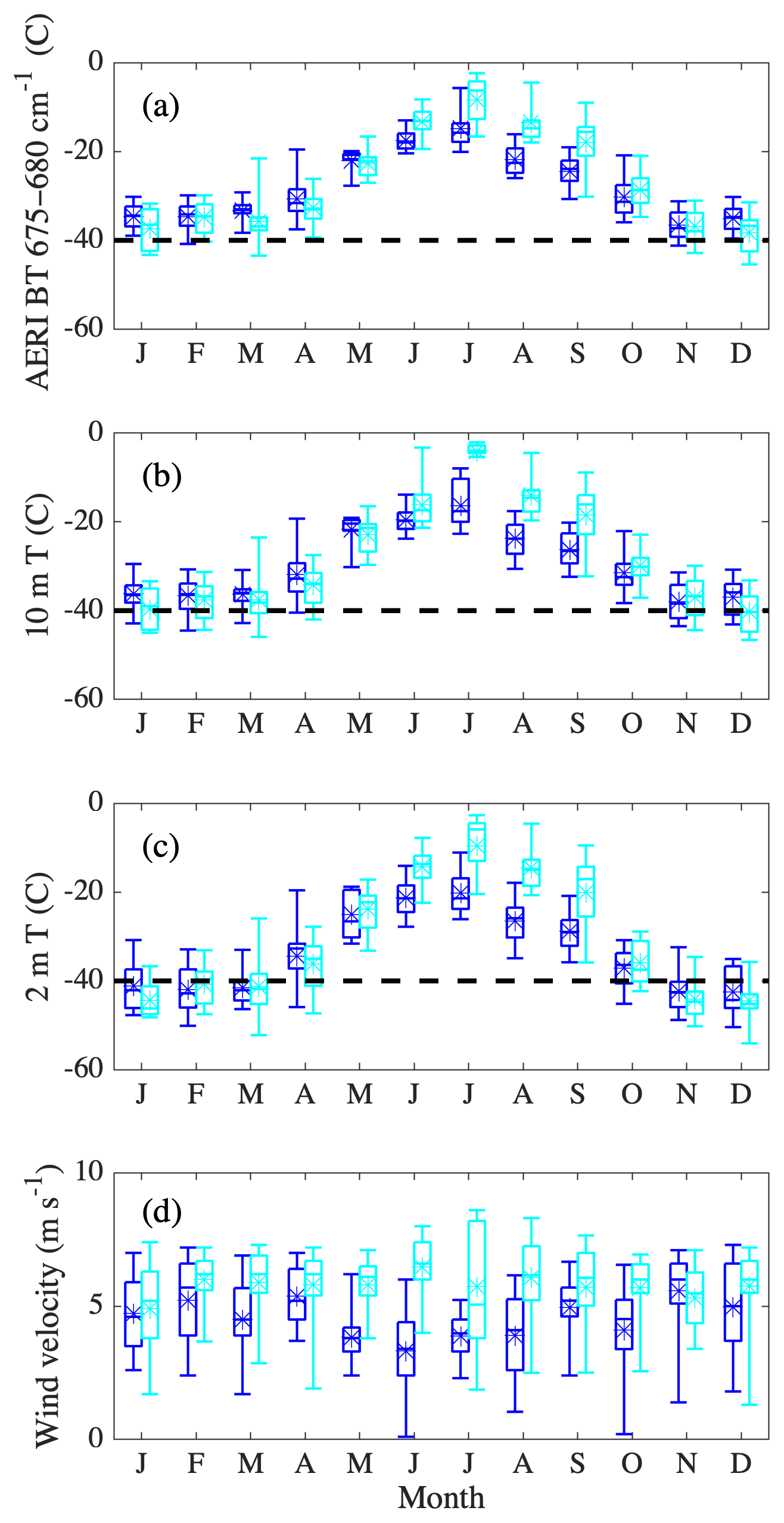
Figure 12Box and whisker plots ( mean, boxes are 25th, 50th, and 75th percentiles, whiskers are 5th and 95th percentiles) for each month for the ice fog category (cyan) and liquid fogs (blue); (a) AERI 675–680 cm−1 brightness temperatures (BT), (b) 10 m air and (c) 2 m air temperature; Panel (d) shows wind velocity at 10 m.
For both ice and liquid identifications in Fig. 12a–c, the temperatures at which they occur are lower in winter and higher in summer. Liquid generally occurs during cooler temperatures than ice in summer and thus the seasonal cycle for liquid is muted compared to that of ice. This is likely a result of diurnally forced radiation fogs occurring during the colder part of the day in summer. There is also a notable difference in the timing of the seasonal cycle with the liquid tending to be warmer than ice in the spring transition and cooler than ice in fall. It is unclear whether this is more closely tied to the seasonal cycle in aerosols (e.g., Schmeisser et al., 2018) or to meteorology. The wind regimes are similar between ice and liquid in winter but liquid fogs in summer occur during particularly calm conditions in association with the diurnal development of stable stratification (Fig. 12d).
5.2 Radiative properties
The impact on the surface radiation budget from the various classifications is evaluated in Fig. 13. The sample sizes in Fig. 13 are analogous to those in Fig. 12. First, distributions of LWCRE for the classes appear alongside those for all observations in Fig. 13a. The peaks for both liquid fog and ice fog are close to 10 W m−2. Both ice and liquid fogs show long tails to larger values and thus the mean is 19.8 (median =14.8) W m−2 for ice and 26.1 (median =18.1) W m−2 for liquid fogs. It is notable that unlike distributions of temperature and microphysics shown earlier, the distributions of LWCRE for ice and liquid are similar. It is therefore possible that a similar amount of downward longwave radiation is needed, when both liquid and ice fogs form, to achieve radiation balance between the surface and the lower atmosphere. However, note that the sample selection was radiative in origin in the first place, and the proportions of missed classifications, in particular at the low end of LWCRE, may be different for the two types. The other ice classes, snow, blowing snow, and a mixture of both, are also plotted in the panel for context. Blowing snow is distributed across the range of LWCRE with the larger values more likely to be associated with higher wind speeds (r2=0.31). Snow also is distributed over a wide range of values, but generally higher than blowing snow alone, which is expected because LWCRE during snowy conditions is associated with a precipitating cloud, whereas blowing snow may occur under otherwise clear skies. When snow and blowing snow occur together, the distribution is clustered near the largest values, a condition mostly associated with storms.
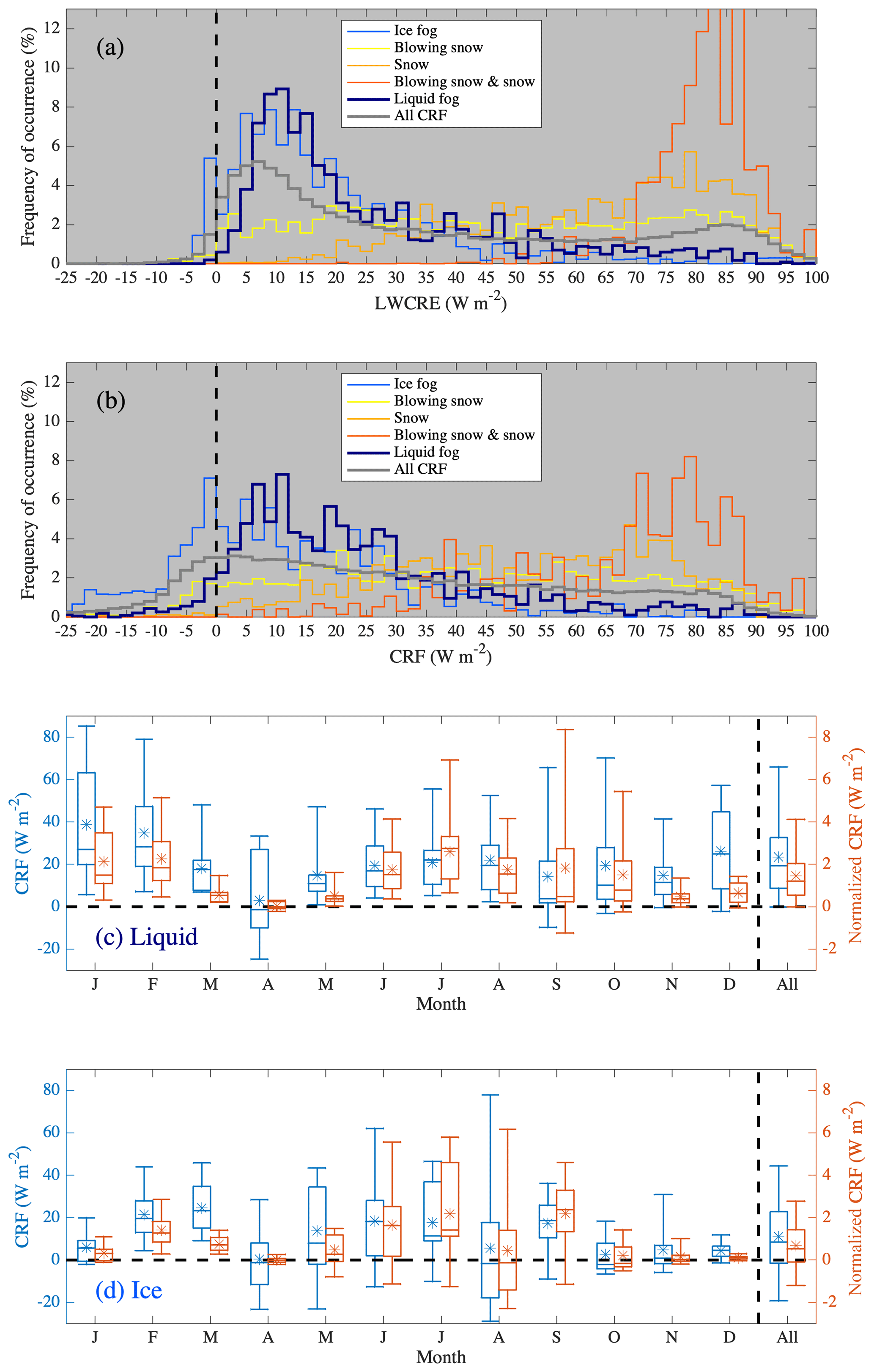
Figure 13Distributions for all seasons for classified data types of (a) longwave cloud radiative effect (LWCRE), defined as the perturbation to the downwelling longwave radiation (LWD) caused by clouds, LWD – LWDclear-sky; (b) Cloud radiative forcing (CRF); (c) For just liquid fog classifications, box and whisker plots ( mean, boxes are 25th, 50th, and 75th percentiles, whiskers are 5th and 95th percentiles) for each month for CRF of identified cases (blue) and CRF normalized by frequency of occurrence of liquid fog (red). Panel (d) as in panel (c) but for the ice fog category.
When the total CRF is considered (Fig. 13b), the results are similar. The forcing is smaller because of the addition of shortwave cloud cooling but only slightly smaller because the high year-round albedo at Summit limits the ability of clouds to cool the surface there (Miller et al., 2015). Notably, there is increased separation in CRF compared to LWCRE between the ice fog class (μ=12.1 W m−2, median =7.9 W m−2) and liquid fog (μ=22.1 W m−2, median =17.1 W m−2). This is because a larger proportion of ice fog occurs at higher sun angles when the shortwave cloud-cooling effect is larger. Therefore, the time of day when liquid fogs typically occur maximizes their net radiative forcing.
Figure 13c and d give the statistics for each month and annually for liquid (Fig. 13c) and ice (Fig. 13d). The annual mean CRF for liquid fogs under otherwise clear skies was 1.5 W m−2 when normalized by the frequency of occurrence. The maximum occurred in July (2.6 W m−2) and the minimum was in April (∼0 W m−2). Due to subsampling, this estimate is probably slightly lower than the total annual CRF from the fogs under all sky types because fogs that were present under optically thin cloud cover may have contributed additional CRF. However, events that were missed for being too thin contributed little radiatively (and consequently, no identification was possible); only a small number of “too thick” (0.8 %) fogs were identified, limiting the influence of this class on the mean CRF; and when ambiguous identifications are included in the analysis (not shown), the annual mean CRF decreases slightly to 1.2 W m−2. For ice, the normalized annual mean is 0.7 W m−2. While the magnitude of the values is similar between ice and liquid, the seasonal cycles are different with ice peaking in July and September (2.2 W m−2). For reference, the mean annual CRF for all sky conditions at Summit is 33 W m−2 and is positive in all months (Miller et al., 2015).
This study analyzed in situ measurements of fog properties over the Greenland Ice Sheet at Summit Station within the predominant southerly-to-westerly wind regimes. At 10 m above the surface, particles associated with snow, blowing snow, fog, or transient particles were observed more than 60 % of the time in all months and over 90 % of the time in winter. Liquid fogs occurring under otherwise clear skies are observed in all months, peaking in September and with a minimum in April. Generally, winter fogs had significantly lower number concentrations (Nc), but only slightly smaller particle sizes compared to summer when mature particles were measured to be typically 20–25 µm in diameter, similar to reports from Borys et al. (1992). Typically, we find that Nc in fogs are <7 cm−3 in winter and between 5 and 20 cm−3 in summer. While these are lower number concentrations than the 30 to 165 cm−3 reported by Borys et al., their study was limited to six well-developed fog cases in August. Their results are actually similar to the well-developed fog analyzed as a case study discussed here in Sect. 4 when Nc was briefly observed above 200 cm−3.
In isolation, the average cloud radiative forcing (CRF) from the liquid fogs when the sky was otherwise clear was 26.1 W m−2 but was much higher in some cases. When normalized by the fractional occurrence when no other clouds were present, the annual average CRF for liquid fog was 1.5 W m−2. As discussed, this estimate may be conservative given subsampling. Given the small overall forcing, it may be more instructive to consider the role of fogs at times in which they occur. Fogs that occur in summer generally appear near the cold times of the diurnal cycle when the surface layer is typically stably stratified. For the 16 June 2013 case, the fog produced enough radiative forcing to increase temperatures by about 5 ∘C. Thus, the development of fog under these conditions constitutes a negative feedback on surface temperature during the coldest part of the day. While surface melt is rare at Summit, at lower elevations where melting produces runoff and is more frequent this damping of surface cooling by fogs could precondition the surface for melting later in the day.
Previous analysis of vapor isotope profiles up to 38 m at Summit (Berkelhammer et al., 2016) indicate that condensation occurs preferentially between 2 and 10 m. In situ observations of particles from the FM100 scattering spectrometers at the two heights support this finding, showing distinct signatures of droplet growth near 10 m and concentration of mature particles near 2 m. The higher number concentrations observed at 2 m may indicate that surface riming is an inefficient process, possibly associated with evaporation of the descending particles. Though most of the droplets nucleated at initiation of the fog in the case studies, some new droplets nucleated later. While recycling of aerosols following droplet evaporation is plausible, Bergin et al. (1995) found that large aerosols (>0.5 µm) occurring in low concentrations were scavenged while populations of smaller aerosols (>0.01 µm) were only partially activated.
The liquid fogs at Summit are supercooled because temperatures are (nearly) always below freezing. However, winter temperatures are frequently near or below −40 ∘C, which is approximately the homogeneous freezing point of liquid. We have observed liquid fogs to develop very close to this threshold, which can only occur in environments that are devoid of ice-forming nuclei. Elevated fog formation at Summit has the important implication that it extends the season under which liquid fogs can form to the winter months. Two out of three scenes containing liquid fogs from November–March occurred when the surface was colder than −40 ∘C with surface skin temperatures as low as −57 ∘C. Particles were large enough to settle out and were observed at 2 m for these cases. We postulate that such fogs were therefore mixed-phase fogs, with a liquid formation layer residing above and feeding a settling layer of frozen ice particles. The resulting surface accumulation may be more likely to behave like light precipitation than rime with respect to surface roughness and has a higher potential to be relofted. Additionally, the lower density of the ice particles compared to their liquid state could serve to reduce their settling rate, while the phase change may buffer the settling particles somewhat from revaporizing, or even reverse the process, as their sublimation rate as ice would be weaker than their evaporation rate as liquid.
The interplay between thermal, dynamical, and microphysical processes, coupled with the significant radiative impact of fogs, highlights that more work is needed to understand the dynamics of the boundary layer during fog events. For example, the multiple fog layers apparent from the sodar record in the wintertime case study are intriguing but will require additional analyses and possibly new measurements in order to ascertain the processes involved in developing and maintaining the distinct layers, as well as to identify the ways they are coupled and what role they may have in regulating the surface mass balance. A complete physical characterization of the fogs also requires detailed observations of aerosols, which were not collected during the period the FM100s operated. While aerosol optical properties are routinely observed at Summit (Schmeisser et al., 2018), additional observations previously only made for brief periods (e.g., Bergin et al., 1995) of number concentration and speciation are necessary for further study. Indeed, such measurements are warranted as the influence of the fogs on climate is likely important for surface melt potential (this work), aerosol cycling (Bergin et al., 1995), and sublimation or deposition processes (Berkelhammer et al., 2016). We anticipate that these processes will act differently at other locations over the Greenland Ice Sheet where different boundary-layer characteristics occur, including wind regimes associated with sloped topography (e.g., katabatic wind), cloud occurrence (e.g., Starkweather, 2004; Cox et al., 2014), and moisture availability. The findings presented here suggest that fogs significantly influence the surface mass and energy budgets over the Greenland Ice Sheet and therefore require consideration when modeling ice sheet boundary-layer processes.
The broadband radiation data were collected by the Swiss Federal Institute, ETH; the data from Miller et al. (2015, 2017) is archived at the NSF Arctic Data Center (ADC), https://doi.org/10.18739/A2Z37J (Shupe and Miller, 2016). Meteorological data collected by NOAA's Global Monitoring Division (GMD) may be accessed from https://www.esrl.noaa.gov/gmd/ (last access: June 2018). The ICECAPS data are available from the ADC from the following DOIs: ceilometer (https://doi.org/10.18739/A2221V; Shupe, 2014a), radar (https://doi.org/10.18739/A2BJ3X; Shupe, 2012a – https://doi.org/10.18739/A2318G; Shupe, 2013a – https://doi.org/10.18739/A2121J; Shupe, 2014b), sodar (https://doi.org/10.18739/A21V2V; Shupe, 2013b), radiosondes (https://doi.org/10.18739/A2X508; Walden and Shupe, 2012 – https://doi.org/10.18739/A2NN44; Walden and Shupe, 2013 – https://doi.org/10.18739/A2WZ18; Walden and Shupe, 2014), AERI (https://doi.org/10.18739/A2TF7R; Walden, 2012a – https://doi.org/10.18739/A2VF6P; Walden, 2012b – https://doi.org/10.18739/A2JZ2J; Walden, 2013a – https://doi.org/10.18739/A29F73; Walden, 2013b – https://doi.org/10.18739/A2PJ65; Walden, 2014), MWR (https://doi.org/10.18739/A22J6K; Turner and Bennartz, 2013 – https://doi.org/10.18739/A2HJ57; Turner and Bennartz, 2014), and MPL (https://doi.org/10.18739/A20R48; Shupe, 2012b – https://doi.org/10.18739/A2MJ55; Shupe, 2013c – https://doi.org/10.18739/A23J5H; Shupe, 2014c). The CIBS data are available from the ADC from the following DOIs: meteorology (https://doi.org/10.18739/A2WW76Z78; Noone et al., 2018a – https://doi.org/10.18739/A21N7XM2W; Noone et al., 2018b – https://doi.org/10.18739/A25D8ND61, Noone et al., 2018c) and cloud probe (https://doi.org/10.18739/A28K74W5W; Noone and Cox, 2019). The sonic anemometer data are available from https://www.esrl.noaa.gov/psd/arctic/observatories/summit/index.html (last access: July 2017).
The supplement related to this article is available online at: https://doi.org/10.5194/acp-19-7467-2019-supplement.
DCN, MB, VPW, MDS, and KS led and collected the observations with assistance from NBM and CJC. CJC led the analysis with contributions from DCN, MB, WDN, NBM, and MDS. CJC prepared the paper with contributions from DCN, MB, MDS, NBM, and VPW.
The authors declare that they have no conflict of interest.
The Department of Energy's Atmospheric Radiation Measurement (ARM) program provided the MPL and ceilometer. We appreciate the CIBS program data management and field efforts of Michael O'Neill (formerly NOAA) and David Schneider (CIRES, NCAR). We acknowledge useful conversations on aerosols with Jessie Creamean (CIRES/NOAA) and instrumentation with Bill Dawson and Matt Freer at Droplet Measurement Technologies (DMT). We appreciate the efforts of David Turner (NOAA), Claire Pettersen (SSEC), Aronne Merrelli (SSEC), and Jonathan Edwards-Opperman (Univ. Oklahoma) in product development for the MWR and MPL datasets. We also appreciate the constructive comments from two anonymous reviewers and the efforts of the technicians at Summit Station and Polar Field Services, who provided high-quality science support and the efforts of the many contributors to the ICECAPS and CIBS research programs.
This research has been supported by the Arctic Research Program of the the NOAA Climate Program Office and the National Science Foundation, Division of Polar Programs (grant nos. 1023574, 1303879, 1314156, 1414314, 1420932).
This paper was edited by Martina Krämer and reviewed by two anonymous referees.
Antonelli, P., Revercomb, H. E., Sromovsky, L. A., Smith, W. L., Knuteson, R. O., Tobin, D. C., Garcia, R. K., Howell, H. B., Huang, H. L., and Best, F. A.: A principal component noise filter for high spectral resolution infrared measurements, J. Geophys. Res.-Atmos., 109, D23102, https://doi.org/10.1029/2004JD004862, 2004.
Bennartz, R., Shupe, M. D., Turner, D. D., Walden, V. P., Steffen, K., Cox, C. J., Kulie, M. S., Miller, N. B., and Pettersen, C.: July 2012 Greenland melt extent enhanced by low-level liquid clouds, Nature, 496, 83–86, https://doi.org/10.1038/nature12002, 2013.
Bergin, M. H., Jaffrezo, J.-L., Davidson, C. I., Dibb, J. E., Pandis, S. N., Hillamo, R., Maenhaut, W., Kuhns, H. D., and Makela, T.: The contributions of snow, fog, and dry deposition to the summer flux anions and cations at Summit, Greenland, J .Geophys. Res., 100, 16275–16288, https://doi.org/10.1029/95JD01267, 1995.
Berkelhammer, M., Noone, D. C., Steen-Larsen, H. C., Bailey, A., Cox, C. J., O'Neill, M. S., Schneider, D., Steffen, K., and White, J. W. C.: Surface-atmosphere decoupling limits accumulation at Summit, Greenland, Sci. Adv., 2, e1501704, https://doi.org/10.1126/sciadv.1501704, 2016.
Borrmann, S., Luo, B., and Mishchenki, M.: Application of the T-Matrix method to the measurement of aspherical (ellipsoidal) particles with forward scatting optical particle counters, J. Aerosol Sci., 31, 789–799, https://doi.org/10.1016/S0021-8502(99)00563-7, 2000.
Borys, R. D., Del Vecchio, D., Jaffrezo, J. L., Dibb, J. E., and Mitchell, D. L.: Field observations, measurements and preliminary results from a study of wet deposition processes influencing snow and ice chemistry at Summit, Greenland, in Precipitation, Scavenging and Atmospheric Surface Exchange, edited by: Schwartz, S. E. and Slinn, W. G. N., 1693–1702, Hemisphere Pub., Philadelphia, USA, 1992.
Braham, R. R.: Snow particle size spectra in lake effect snows, J. Atmos. Sci., 29, 200–207, https://doi.org/10.1175/1520-0450(1990)029<0200:SPSSIL>2.0.CO;2, 1990.
Castellani, B., Shupe, M. D., Hudak, D. R., and Sheppard, B .E.: The annual cycle of snowfall at Summit, Greenland, J. Geophys. Res.-Atmos., 120, 6654–6668, https://doi.org/10.1002/2015JD023072, 2015.
Clough, S. A., Shepard, M .W., Mlawer, E. J., Delamere, J. S., Iacono, M. J., Cady-Pereira, K., Boukabara, S., and Brown, P. D.: Atmospheric radiative transfer modeling: a summary of the AER codes, short communications, J. Quant. Spectrosc. Ra., 91, 233–244, https://doi.org/10.1016/j.jqsrt.2004.05.058, 2005.
Cox, C. J., Walden, V. P., Compo, G. P., Rowe, P. M., Shupe, M. D., and Steffen, K.: Downwelling longwave flux over Summit, Greenland, 2010–2012: Analysis of surface-based observations and evaluation of ERA-Interim using wavelets, J. Geophys. Res.-Atmos., 119, 12317–12337, https://doi.org/10.1002/2014JD021975, 2014.
Cox, C. J., Walden, V. P., Rowe, P. M., and Shupe, M. D.: Humidity trends imply increased sensitivity to clouds in a warming Arctic, Nat. Commun., 6, 10117, https://doi.org/10.1038/ncomms10117, 2015.
Crane, R. G. and Anderson, M. R.: Satellite discrimination of snow/cloud surfaces, Int. J. Remote Sens., 5, 213–223, https://doi.org/10.1080/01431168408948799, 1984.
Dye, J. E. and Baumgardner, D.: Evaluation of the forward scattering spectrometer probe, I: Electronic and optical studies, J. Atmos. Ocean Tech., 1, 329–344, https://doi.org/10.1175/1520-0426(1984)001<0329:EOTFSS>2.0.CO;2, 1984.
Edwards-Opperman, J., Cavallo, S., and Turner, D. D.: The occurrence and properties of long-lived liquid bearing clouds over the Greenland Ice Sheet and their relationship to the North Atlantic Oscillation, J. Appl. Meteorol. Clim., 57, 921–935, https://doi.org/10.1175/JAMC-D-17-0230.1, 2018.
Garrett, T. J. and Zhao, C.: Increased Arctic cloud longwave emissivity associated with pollution from mid-latitudes, Nature, 440, 787–789, https://doi.org/10.1038/nature04636, 2006.
Gossart, A., Souverijns, N., Gorodetskaya, I. V., Lhermitte, S., Lenaerts, J. T. M., Schween, J. H., Mangold, A., Laffineur, Q., and van Lipzig, N. P. M.: Blowing snow detection from ground-based ceilometers: application to East Antarctica, The Cryosphere, 11, 2755–2772, https://doi.org/10.5194/tc-11-2755-2017, 2017.
Gultepe, I. and Isaac, G. A.: Aircraft observations of cloud droplet number concentration: Implications for climate studies, Q. J. Roy. Meteor. Soc., 130, 2377–2390, https://doi.org/10.1256/qj.03.120, 2004.
Gultepe, I., Isaac, G. A., and Cober, S. G.: Cloud microphysical characteristics versus temperature for three Canadian field projects, Ann. Geophys., 20, 1891–1898, https://doi.org/10.5194/angeo-20-1891-2002, 2002.
Gultepe, I. R., Tardif, S. C., Michaelides, J., Cermak, A., Bott, A., Bendix, J., Müller, M. D., Pagaowski, M., Hansen, B., Ellrod, G., Jacobs, W., Toth, G., and Tober, S. G.: Fog research: A review of past achievements and future perspectives, Pure Appl. Geophys., 164, 1121–1159, https://doi.org/10.1007/s00024-007-0211-x, 2007.
Gultepe, I. R., Zhou, B., Milbrandt, J., Bott, A., Li, Y., Heymsfield, A. J., Ferrier, B., Ware, R., Pavolonis, M., Kuhn, T., Gurka, J., Liu, P., and Cermak, J.: A review on ice fog measurements and modeling, Atmos. Res., 151, 2–19, https://doi.org/10.1016/j.atmosres.2014.04.014, 2015.
Hoch, S. W., Calanca, P., Philipona, R., and Ohmura, A.: Year-round observation of longwave radiative flux divergence in Greenland, J. Appl. Meteorol. Clim., 46, 1469–1479, https://doi.org/10.1175/JAM2542.1, 2007.
Houghton, H. G.: Physical Meteorology, MIT Press, https://doi.org/10.1002/qj.49711247218, 1985.
Knuteson, R. O., Revercomb, H. E., Best, F. A., Ciganovich, N. C., Dedecker, R. G., Dirkx, T. P., Ellington, S. C., Feltz, W. F., Garcia, R. K., Howell, H. B., Smith, W. L., Short, J. F., and Tobin, D. C.: Atmospheric Emitted Radiance Interferometer: Part I: Instrument design, J. Atmos. Ocean. Tech., 21, 1763–1776, J. https://doi.org/10.1175/JTECH-1662.1, 2004a.
Knuteson, R. O., Revercomb, H. E., Best, F. A., Ciganovich, N. C., Dedecker, R. G., Dirkx, T. P., Ellington, S. C., Feltz, W. F., Garcia, R. K., Howell, H. B., Smith, W. L., Short, J. F., and Tobin, D. C.: Atmospheric Emitted Radiance Interferometer: Part II: Instrument performance, J. Atmos. Ocean. Tech., 21, 1777–1789, J. https://doi.org/10.1175/JTECH-1663.1, 2004b.
Li, L. and Pomeroy, J. W.: Probability of occurrence of blowing snow, J. Geophys. Res.-Atmos., 102, 21955–21964, https://doi.org/10.1029/97JD01522, 1997.
Lynch, D. K. and Schwartz, P.: Rainbows and fogbows, Appl. Optics, 30, 3415–3420, https://doi.org/10.1364/AO.30.003415,1991.
Miller, N. B., Turner, D. D., Bennartz, R., Shupe, M. D., Kulie, M. S., Cadeddu, M. P., and Walden, V. P.: Surface-based inversions above central Greenland, J. Geophys. Res.-Atmos., 118, 495–506, https://doi.org/10.1029/2012JD018867, 2013.
Miller, N. B., Shupe, M. D., Cox, C. J., Walden, V. P., Turner, D. D., and Steffen, K.: Cloud radiative forcing at Summit, Greenland, J. Climate, 28, 6267–6280, https://doi.org/10.1175/JCLI-D-15-0076.1, 2015.
Miller, N. B., Shupe, M. D., Cox, C. J., Noone, D., Persson, P. O. G., and Steffen, K.: Surface energy budget responses to radiative forcing at Summit, Greenland, The Cryosphere, 11, 497–516, https://doi.org/10.5194/tc-11-497-2017, 2017.
Moran, K. P., Martner, B. E., Post, M. J., Kropfli, R. A., Welsh, D. C., and Widener, K. B.: An unattended cloud-profiling radar for use in climate research, B. Am. Meteorol. Soc., 79, 443–455, https://doi.org/10.1175/1520-0477(1998)079<0443:AUCPRF>2.0.CO;2, 1998.
Nakanishi, M.: Large-Eddy Simulation of radiation fog, Bound.-Lay. Meteorol., 94, 461–493, https://doi.org/10.1023/A:1002490423389, 2000.
Neff, W., Helmig, D., Grachev, A., and Davis, D.: A study of boundary layer behavior associated with high NO concentrations at the South Pole using a minisodar, tethered balloon, and sonic anemometer, Atmos. Environ., 42, 2762–2779, https://doi.org/10.1016/j.atmosenv.2007.01.033, 2008.
Nghiem, S. V., Hall, D. K., More, T. L., Tedesco, M., Albert, M. R., Keegan, K., Shuman, C. A., DiGirolamo, N. E., and Neumann, G.: The extreme melt across the Greenland ice sheet in 2012, Geophys. Res. Lett., 39, L20502, https://doi.org/10.1029/2012GL053611, 2012.
Noone, D. C. and Cox, C. J.: Summit, Greenland, Meteorology and Snow Temperatures: 2011–2014, Arctic Data Center, https://doi.org/10.18739/A28K74W5W, 2019.
Noone, D. C., Cox, C. J., Berkelhammer, M., and O'Neill, M.: Tower meteorology at multiple heights and snow temperature, Summit, Greenland, 2011–2014, Arctic Data Center, https://doi.org/10.18739/A2WW76Z78, 2018a.
Noone, D. C., Cox, C. J., Berkelhammer, M., and O'Neill, M.: Tower meteorology at multiple heights and snow temperature, Summit, Greenland, 2013–2014, Arctic Data Center, https://doi.org/10.18739/A21N7XM2W, 2018b.
Noone, D. C., Cox, C. J., Berkelhammer, M., and O'Neill, M.: Tower meteorology at multiple heights and snow temperature, Summit, Greenland, 2011–2012, Arctic Data Center, https://doi.org/10.18739/A25D8ND61, 2018c.
Pettersen, C., Bennartz, R., Merrelli, A. J., Shupe, M. D., Turner, D. D., and Walden, V. P.: Precipitation regimes over central Greenland inferred from 5 years of ICECAPS observations, Atmos. Chem. Phys., 18, 4715–4735, https://doi.org/10.5194/acp-18-4715-2018, 2018.
Pinnick, R. and Auvermann, H.: Response characteristics of Knollenberg light-scattering aerosol counters, J. Aerosol Sci., 10, 55–74, https://doi.org/10.1016/0021-8502(79)90136-8, 1979.
Pruppacher, H. R. and Klett, J. D.: Microphysics of Clouds and Precipitation, 2nd ed., Springer Science & Business Media, London, UK, 954 pp., https://doi.org/10.1007/978-0-306-48100-0, 2010.
Schmeisser, L., Backman, J., Ogren, J. A., Andrews, E., Asmi, E., Starkweather, S., Uttal, T., Fiebig, M., Sharma, S., Eleftheriadis, K., Vratolis, S., Bergin, M., Tunved, P., and Jefferson, A.: Seasonality of aerosol optical properties in the Arctic, Atmos. Chem. Phys., 18, 11599–11622, https://doi.org/10.5194/acp-18-11599-2018, 2018.
Shupe, M.: Millimeter Cloud Radar measurements taken at Summit Station, Greenland, 2012, Arctic Data Center, https://doi.org/10.18739/A2BJ3X, 2012a.
Shupe, M.: Micropulse lidar (MPL) measurements taken at Summit Station, Greenland, 2012, Arctic Data Center, https://doi.org/10.18739/A20R48, 2012b.
Shupe, M.: Millimeter Cloud Radar measurements taken at Summit Station, Greenland, 2013, Arctic Data Center, https://doi.org/10.18739/A2318G, 2013a.
Shupe, M.: SOnic Detection And Ranging (SODAR) measurements taken at Summit Station, Greenland, 2013, Arctic Data Center, https://doi.org/10.18739/A21V2V, 2013b.
Shupe, M.: Micropulse lidar (MPL) measurements taken at Summit Station, Greenland, 2013, Arctic Data Center, https://doi.org/10.18739/A2MJ55, 2013c.
Shupe, M.: Ceilometer Cloud Base Height Measurements at Summit Station, Greenland, 2014, Arctic Data Center, https://doi.org/10.18739/A2221V, 2014a.
Shupe, M.: Millimeter Cloud Radar measurements taken at Summit Station, Greenland, 2014, Arctic Data Center, https://doi.org/10.18739/A2121J, 2014b.
Shupe, M.: Micropulse lidar (MPL) measurements taken at Summit Station, Greenland, 2014, Arctic Data Center, https://doi.org/10.18739/A23J5H, 2014c.
Shupe, M. D. and Intrieri, J. M.: Cloud radiative forcing of the Arctic surface: Influence of cloud properties, surface albedo, and solar zenith angle, J. Climate, 17, 616–628, https://doi.org/10.1175/1520-0442(2004)017<0616:CRFOTA>2.0.CO;2, 2004.
Shupe, M. D. and Miller, N. B.: Surface-energy budget at Summit, Greenland, NSF Arctic Data Center, https://doi.org/10.18739/A2Z37J, 2016.
Shupe, M. D., Walden, V. P., Eloranta, E., Uttal, T., Campbell, J. R., Starkweather, S. M., and Shiobara, M.: Clouds at Arctic atmospheric observatories. Part I: Occurrence and macrophysical properties, J. Appl. Meteorol. Clim., 50, 626–644, https://doi.org/10.1175/2010JAMC2467.1, 2011.
Shupe, M. D., Turner, D. D., Walden, V. P., Bennartz, R., Cadeddu, M. P., Castellani, B. B., Cox, C. J., Hudak, D. R., Kulie, M. S., Miller, N. B., Neely III, R. R., Neff, W. D., and Rowe, P. M.: High and Dry: New observations of tropospheric and cloud properties above the Greenland ice sheet, B. Am. Meteorol. Soc., 94, 169–186, https://doi.org/10.1175/BAMS-D-11-00249.1, 2013.
Spiegel, J. K., Zieger, P., Bukowiecki, N., Hammer, E., Weingartner, E., and Eugster, W.: Evaluating the capabilities and uncertainties of droplet measurements for the fog droplet spectrometer (FM-100), Atmos. Meas. Tech., 5, 2237–2260, https://doi.org/10.5194/amt-5-2237-2012, 2012.
Starkweather, S. M.: Characteristics of cloud cover and its radiative impacts over high elevations of the Greenland ice sheet, PhD dissertation, Dep. of Atmos. Oceanic Sci., Univ. of Colorado, Boulder, USA, 2004.
Strabala, K. I., Ackerman, S. A., and Menzel, W. P.: Cloud properties inferred from 8–12-µm data, J. Appl. Meteorol., 33, 212–229, https://doi.org/10.1175/1520-0450(1994)033<0212:CPIFD>2.0.CO;2, 1994.
Thuman, W. C. and Robinson, E.: Studies on Alaskan ice-fog particles, J. Meteorol., 11, 151–156, https://doi.org/10.1175/1520-0469(1954)011<0151:SOAIFP>2.0.CO;2, 1954.
Tjernström, M.: The summer Arctic boundary layer during the Arctic Ocean Experiments 2001 (AOE-2001), Bound.-Lay. Meteorol., 117, 5–36, https://doi.org/10.1007/s10546-004-5641-8, 2005.
Turner, D. D.: Arctic mixed-phase cloud properties from AERI lidar observations: Algorithm and results from SHEBA, J. Appl. Meteorol., 44, 427–444, https://doi.org/10.1175/JAM2208.1, 2005.
Turner, D. and Bennartz, R.: Microwave Radiometer measurements of sky brightness temperature taken at Summit Station, Greenland, 2013, Arctic Data Center, https://doi.org/10.18739/A22J6K, 2013.
Turner, D. and Bennartz, R.: Microwave Radiometer measurements of sky brightness temperature taken at Summit Station, Greenland, 2014, Arctic Data Center, https://doi.org/10.18739/A2HJ57, 2014.
Turner, D. D., Ackerman, S. A., Baum, B. A., Revercomb, H. E., and Yang, P.: Cloud phase determination using ground-based AERI observations at SHEBA, J. Appl. Meteorol., 42, 701–715, https://doi.org/10.1175/1520-0450(2003)042<0701:CPDUGA>2.0.CO;2, 2003.
Turner, D. D., Knuteson, R. O., Revercomb, H. E., Lo, C., and Dedecker, R. G.: Noise reduction of Atmospheric Emitted Radiance Interferometer (AERI) observations using Principal Component Analysis, J. Atmos. Ocean. Tech., 23, 1223–1238, https://doi.org/10.1175/JTECH1906.1, 2006.
Turner, D. D., Clough, S. A., Liljegren, J .C., Clothiaux, E. E., Cady-Pereira, K. E., and Gaustad, K. L.: Retrieving liquid water path and precipitable water vapor from the Atmospheric Radiation Measurement (ARM) microwave radiometers, IEEE T. Geosci. Remote, 45, 3680–3690, https://doi.org/10.1109/TGRS.2007.903703, 2007.
Walden, V. P.: Polar atmospheric emitted radiance interferometer measurements, Summit Station, Greenland, July–December 2012, Arctic Data Center, https://doi.org/10.18739/A2TF7R, 2012a.
Walden, V. P.: Polar atmospheric emitted radiance interferometer measurements, Summit Station, Greenland, January–June 2012, Arctic Data Center, https://doi.org/10.18739/A2VF6P, 2012b.
Walden, V. P.: Polar atmospheric emitted radiance interferometer measurements, Summit Station, Greenland, January–June 2013, Arctic Data Center, https://doi.org/10.18739/A2JZ2J, 2013a.
Walden, V. P.: Polar atmospheric emitted radiance interferometer measurements, Summit Station, Greenland, July–December 2013, Arctic Data Center, https://doi.org/10.18739/A29F73, 2013b.
Walden, V. P.: Polar atmospheric emitted radiance interferometer measurements, Summit Station, Greenland, January–June 2014, Arctic Data Center, https://doi.org/10.18739/A2PJ65, 2014.
Walden, V. P. and Shupe, M.: Radiosonde temperature and humidity profiles taken at Summit Station, Greenland, 2012, Arctic Data Center, https://doi.org/10.18739/A2X508, 2012.
Walden, V. P. and Shupe, M.: Radiosonde temperature and humidity profiles taken at Summit Station, Greenland, 2013, Arctic Data Center, https://doi.org/10.18739/A2NN44, 2013.
Walden, V. P. and Shupe, M.: Radiosonde temperature and humidity profiles taken at Summit Station, Greenland, 2014, Arctic Data Center, https://doi.org/10.18739/A2WZ18, 2014.