the Creative Commons Attribution 4.0 License.
the Creative Commons Attribution 4.0 License.
 | 29 May 2019
Large-eddy simulation of radiation fog with comprehensive two-moment bulk microphysics: impact of different aerosol activation and condensation parameterizations
Johannes Schwenkel
Björn Maronga
In this paper we study the influence of the cloud microphysical parameterization, namely the effect of different methods for calculating the supersaturation and aerosol activation, on the structure and life cycle of radiation fog in large-eddy simulations. For this purpose we investigate a well-documented deep fog case as observed at Cabauw (the Netherlands) using high-resolution large-eddy simulations with a comprehensive bulk cloud microphysics scheme. By comparing saturation adjustment with a diagnostic and a prognostic method for calculating supersaturation (while neglecting the activation process), we find that, even though assumptions for saturation adjustment are violated, the expected overestimation of the liquid water mixing ratio is negligible. By additionally considering activation, however, our results indicate that saturation adjustment, due to approximating the underlying supersaturation, leads to a higher droplet concentration and hence significantly higher liquid water content in the fog layer, while diagnostic and prognostic methods yield comparable results. Furthermore, the effect of different droplet number concentrations is investigated, induced by using different common activation schemes. We find, in line with previous studies, a positive feedback between the droplet number concentration (as a consequence of the applied activation schemes) and strength of the fog layer (defined by its vertical extent and amount of liquid water). Furthermore, we perform an explicit analysis of the budgets of condensation, evaporation, sedimentation and advection in order to assess the height-dependent contribution of the individual processes on the development phases.


The prediction of fog is an important part of the estimation of hazards and efficiency in traffic and economy (Bergot, 2013). The annual damage caused by fog events is estimated to be the same as the amount caused by winter storms (Gultepe et al., 2009). Despite improvements in numerical weather prediction (NWP) models, the quality of fog forecasts is still unsatisfactory. The explanation for this is obvious: fog is a meteorological phenomenon influenced by a multitude of complex physical processes. Namely, these processes are radiation, turbulent mixing, atmosphere–surface interactions and cloud microphysics (hereafter referred to as microphysics), which interact on different scales (e.g., Gultepe et al., 2007; Haeffelin et al., 2010). The key issue for improving fog prediction in NWP models is to resolve the relevant processes and scales explicitly or – if that is not possible – to parameterize them in an appropriate way.
In recent years, various studies focused on the influence of microphysics on fog. In particular, the activation of aerosols (hereafter simply referred to as activation), which determines how many aerosols at a certain supersaturation get activated and hence can grow into cloud drops, is a key process and thus of special interest (e.g., Bott, 1991; Hammer et al., 2014; Boutle et al., 2018).
Stolaki et al. (2015) investigated and compared the influence of aerosols on the life cycle of a radiation fog event while using the one-dimensional (1-D) mode of the MESO-NH model with a two-moment warm microphysics scheme, after Geoffroy et al. (2008) and Khairoutdinov and Kogan (2000), and included an activation parameterization after Cohard et al. (1998). In other fog studies, using single-column models, different activation schemes such as the simple Twomey power law activation in Bott and Trautmann (2002) and the scheme of Abdul-Razzak and Ghan (2000)(see Zhang et al., 2014) were applied. Furthermore, also more advanced methods such as sectional models have been used for an appropriate activation representation. Maalick et al. (2016) used the Sectional Aerosol module for Large Scale Applications (SALSA; Kokkola et al., 2008) in two-dimensional (2-D) studies for a size-resolved activation. Mazoyer et al. (2017) conducted, similar to Stolaki et al. (2015), simulations for the ParisFog Experiment with the MESO-NH model (for more information to the MESO-NH model, see Lac et al., 2018), but using the three-dimensional (3-D) large-eddy simulation (LES) mode and focusing on the drag effect of vegetation on droplet deposition. For the fog microphysics, they used the activation parameterizations after Cohard et al. (2000) in connection with saturation adjustment. As outlined above, several different activation parameterizations have been employed for simulating radiation fog. This raises the question how different methods affect the structure and life cycle of radiation fog. Furthermore, schemes that parameterize activation based on updrafts (typically done in NWP models) might fail for fog. Such schemes derive supersaturation as a function of vertical velocity, which is valid for convective clouds that are forced by surface heating but not for radiation fog, which is mainly driven by longwave radiative cooling in its development and mature phase (Maronga and Bosveld, 2017; Boutle et al., 2018).
Although great progress has been made to understand different microphysical processes in radiation fog based on numerical experiments, turbulence as a key process has been either fully parameterized (single-column models) or oversimplified (2-D LES). Since turbulence is a fundamentally 3-D process, the full complexity of all relevant mechanisms can only be reproduced with 3-D LESs (Nakanishi, 2000).
Moreover, a disadvantage of most former studies is the use of saturation adjustment, which implies that supersaturations are immediately removed within one time step. This approach is only valid when the timescale for diffusion of water vapor (on the order of 2–5 s) is much smaller than the model time step. This is the case in large-scale models where time steps are on the order of 1 min, but in LES of radiation fog, time steps easily go down to split seconds so that the assumption made for saturation adjustment is violated and might lead to excessive condensation (e.g., Lebo et al., 2012; Thouron et al., 2012). As a follow-up to these studies, which investigated the influence of different supersaturation calculations for deep convective cloud and stratocumulus, the present work investigates the effect of saturation adjustment on radiation fog.
As Mazoyer et al. (2017) and Boutle et al. (2018) stated that both LES and NWP models tend to overestimate the liquid water content and the droplet number concentration for radiation fog, the following questions are derived from these shortcomings:
- i.
Is saturation adjustment appropriate as it crucially violates the assumption of equilibrium? How large is the effect of different methods to calculate supersaturation on diffusional growth of fog droplets?
- ii.
As the number of activated fog droplets is essentially determined by the supersaturation, how large is the effect of different supersaturation modeling approaches on aerosol activation and thus on the strength and life cycle of radiation fog (see Thouron et al., 2012)?
- iii.
What is the impact of different activation schemes on the fog life cycle for a given aerosol environment?
In the present paper we will address the above research questions by employing idealized high-resolution LESs with atmospheric conditions based on an observed typical deep fog event with continental aerosol conditions at Cabauw (the Netherlands).
The paper is organized as follows: Sect. 2 outlines the methods used, that is, the LES modeling framework and the microphysics parameterizations used. Section 3 provides an overview of the simulated cases and model setup, while results are presented in Sect. 4. Conclusions are given in Sect. 5.
This section will outline the used LES model and the treatment of radiation and land–surface interactions, followed by a more detailed description of the bulk microphysics implemented in the Parallelized Large-Eddy Simulation Model (PALM) and the extensions made in the scope of the present study.
2.1 LES model with embedded radiation and land surface model
In this study the LES PALM (Maronga et al., 2015; revision 2675 and 3622) was used with additional extensions in the microphysics parameterizations. PALM has been successfully applied to simulate the stable boundary layer (BL) (e.g., during the first intercomparison of LES for stable BL – GABLS; Beare et al., 2006) as well as radiation fog (Maronga and Bosveld, 2017). The model is based on the incompressible Boussinesq-approximated Navier–Stokes equations and prognostic equations for total water mixing ratio, potential temperature and subgrid-scale turbulent kinetic energy (TKE). PALM is discretized in space using finite differences on a Cartesian grid. For the non-resolved eddies, a 1.5-order flux–gradient subgrid closure scheme after Deardorff (1980) is applied, which includes the solution of an additional prognostic equation for the subgrid-scale TKE. Moreover, the discretization for space and time is done by a fifth-order advection scheme after Wicker and Skamarock (2002) and a third-order Runge–Kutta time-step scheme (Williamson, 1980), respectively. The interested reader is referred to Maronga et al. (2015) for a detailed description of the PALM.
In order to account for radiative effects on fog and the Earth's surface energy balance, the radiation code RRTMG (Clough et al., 2005) has been recently coupled to PALM, running as an independent single-column model for each vertical column of the LES domain. RRTMG calculates the radiative fluxes (shortwave and longwave) for each grid volume while considering profiles of pressure, temperature, humidity, liquid water, the droplet number concentration (nc) and the effective droplet radius (reff). Compared to the precursor study of Maronga and Bosveld (2017), improvements in the microphysics parameterization introduced in the scope of the present study allow a more realistic calculation of the fog's radiation budget, as nc is now represented as a prognostic quantity instead of the previously fixed value specified by the user. This involves an improved calculation of reff, entering RRTMG, which is given as
where ql is the liquid water mixing ratio, ρ is the density of air, ρl is the density of water and σg=1.3 is the geometric standard deviation of the droplet distribution. The effective droplet radius is the main interface between the optical properties of the cloud and the radiation model RRTMG. Note that 3-D radiation effects of the cloud are not implemented in this approach, which, however, could affect the fog development at the lateral edges during formation and dissipation phases when no homogeneous fog layer is present. As radiation calculations traditionally require enormous computational time, the radiation code is called at fixed intervals on the order of 1 min.
Moreover, PALM's land surface model (LSM) is used to calculate the surface fluxes of sensible and latent heat. The LSM consists of a multi-layer soil model, predicting soil temperature and soil moisture, as well as a solver for the energy balance of the Earth's surface using a resistance parameterization. The implementation is based on the ECMWF-IFS land surface parameterization (H-TESSEL) and its adaptation in the DALES model (Heus et al., 2010). A description of the LSM and a validation of the model system for radiation fog are given in Maronga and Bosveld (2017).
2.2 Bulk microphysics
As a part of this study, the two-moment microphysics scheme of Seifert and Beheng (2001) and Seifert et al. (2006) implemented in PALM, basically only predicting the rain droplet number concentration (nr) and cloud water mixing (qr), was extended by prognostic equations for nc and the cloud water mixing ratio (qc). The scheme of Seifert and Beheng (2001) and Seifert et al. (2006) is based on the separation of the cloud and rain droplet scale by using a radius threshold of 40 µm. This separation is mainly used for parameterizing coagulation processes by assuming different distribution functions for cloud and rain droplets. However, as collision and coalescence are weak in fog due to small average droplet radii, the production of rain droplets is negligible. Consequently, only the number concentration and mixing ratio of droplets (containing all liquid water and thus abbreviated with ql here) are considered in the following. The budgets of the cloud water mixing ratio and number concentration are given by
The terms on the right-hand side represent the decrease or increase by advection, activation, diffusional growth, autoconversion, accretion and sedimentation (from left to right). Following Ackerman et al. (2009), cloud water sedimentation is parameterized, assuming that droplets have a log-normal distribution and follow a Stokes regime. This results in a sedimentation flux of
with the parameter m−1 s−1 (Geoffroy et al., 2010). The main focus of this paper is to study the effect of different microphysical parameterizations of activation and condensation processes on microphysical and macroscopic properties of radiation fog. Those different activation and supersaturation parameterizations will be discussed in the following.
2.2.1 Activation
It is well known that the aerosol distribution and the activation process are of great importance for the life cycle of fog (e.g., Gultepe et al., 2007). The amount of activated aerosols determines the number concentration of droplets within the fog, which, in turn, has a significant influence on radiation through optical thickness as well as on sedimentation and consequently affects macroscopic properties of the fog, like, for instance, its vertical extent. For these reasons, a sophisticated treatment of the activation process is an essential prerequisite for the simulation of radiation fog. Several activation parameterizations for bulk microphysics models have been proposed in literature. In this work, three of these activation schemes were compared with each other in order to quantify their effect on the development of a radiation fog event. The schemes considered in this scope are the activation scheme of Twomey (1959), which was used, for example, by Bott and Trautmann (2002) to simulate radiation fog, the scheme of Cohard et al., 1998 (used by, for example, Stolaki et al., 2015; Mazoyer et al., 2017), and the one by Khvorostyanov and Curry (2006). The latter two represent an empirical and analytical extension of Twomey's scheme, respectively. Consequently, these parameterizations are frequently termed Twomey-type parameterizations that have the following form:
where NCCN values are the number of activated cloud condensation nuclei (CCN), N0 and k are parameters depending on the aerosol distribution, and s is the supersaturation. The three parameterizations considered in the present study are variations of Eq. (5) differing in mathematical complexity:
-
Twomey (1959). The power law expression (Eq. 5) is well known and has been used for decades to estimate the number of activated aerosols for a given air mass in dependence of the supersaturation. A weakness of this approach is that the parameters N0 and k are usually assumed to be constant and are not directly linked to the microphysical properties. Furthermore, this relationship creates an unbounded number of CCN at high supersaturations.
-
Cohard et al. (1998). This extended Twomey's power law expression by using a more realistic four-parameter CCN activation spectrum as shaped by the physiochemical properties of the accumulation mode. Although an extension to the multi-modal representation of an aerosol spectrum would be possible, all relevant aerosols that are activated in typical supersaturations within clouds and especially fog are represented in the accumulation mode (Cohard et al., 1998; Stolaki et al., 2015). Following Cohard et al. (1998) and Cohard and Pinty (2000), the activated CCN number concentration is expressed by
where C is proportional to the total number concentration of CCN that is activated when supersaturation s tends to infinity. Beside k, the parameters μ and β are adjustable shape parameters associated with the characteristics of the aerosol size spectrum such as the geometric mean radius and the geometric standard deviation as well as with chemical composition and solubility of the aerosols. Thus, in contrast to the original Twomey approach, the effect of physiochemical properties on the aerosol spectrum are taken into account.
-
Khvorostyanov and Curry (2006). This found an analytical solution to express the activation spectrum using Köhler theory. Therein, it is assumed that the dry aerosol spectrum follows a log-normal size distribution of aerosol fd:
Here, rd is the dry aerosol radius, Nt is the total number of aerosols, σd is the dispersion of the dry aerosol spectrum and rd0 is the mean radius of the dry particles. The number of activated CCN as a function of supersaturation s is then given by
where erf is the Gaussian error function, and
In this case, AK is the Kelvin parameter and b and β depend on the chemical composition and physical properties of the soluble part of the dry aerosol.
Since prognostic equations were neither considered for the aerosols nor for their sources and sinks, a fixed aerosol background concentration was prescribed by setting parameters N0, C and Nt for the three activation schemes. The different nomenclature of the aerosol background concentration is based on the nomenclature used in the original literature.
The activation rate is then calculated as
where nc is the number of previously activated aerosols that are assumed to be equal to the number of pre-existing droplets and Δt is the length of the model time step. Note that this method does not take into account reduction of CCN. However, this error can be neglected, since processes like aerosol washout and dry deposition are of minor importance for radiation fog. For all activation schemes it is assumed that every activated CCN becomes a droplet with an initial radius of 1 µm. This results in a change of liquid water, which is considered by the condensation scheme and is described in the next section. Furthermore, we performed a sensitivity study with initial radii of 0.5 to 2 µm, which showed that the choice of the initial radius had no impact on the results (not shown). This is consistent with the findings of Khairoutdinov and Kogan (2000) and Morrison and Grabowski (2007).
2.2.2 Condensation and supersaturation calculation
The representation of diffusional growth, evaporation and calculating the underlying supersaturation (which is the main driver for activation) is one of the fundamental tasks of cloud physics. Three different methods have been evaluated and widely discussed in the scientific community. Namely, these are the saturation adjustment scheme, the diagnostic scheme, where the supersaturation is diagnosed by the prognostic fields of temperature and water vapor, and a prognostic method for calculating the supersaturation following, for example, Clark (1973), Morrison and Grabowski (2007), and Lebo et al. (2012). Basically, the supersaturation is given by , while the absolute supersaturation (or water vapor surplus) is defined as , where qv is the water vapor mixing ratio and qs is the saturation mixing ratio. In the following, these three methods are briefly reviewed.
-
Saturation adjustment. In many microphysical models, a saturation adjustment scheme is applied. The basic idea of this scheme is that all supersaturation is removed within one model time step and supersaturations are thus neglected. Saturation adjustment thus potentially leads to excessive condensation. Despite the many years of application of this scheme, its impact on microphysical processes is discussed controversially (e.g., Morrison and Grabowski, 2008; Thouron et al., 2012; Lebo et al., 2012). Saturation adjustment might hence especially be a source of error in fog simulations, where very small time steps are used due to small grid spacings, as already discussed. Using the saturation adjustment scheme, ql represents a diagnostic value calculated by means of
where q is the total water mixing ratio. The saturation mixing ratio, which is a function of temperature, is approximated in a first step by
where Tl is the liquid water temperature and p is pressure. Rd and Rv are the specific gas constants for dry air and water vapor, respectively. For the saturation vapor pressure (es) an empirical relationship of Bougeault (1981) is used. In a second step, qs is corrected using a first-order Taylor series expansion of qs:
with
where cp is the specific heat of dry air at constant pressure and Lv is the latent heat of vaporization. As previously mentioned, in each model time step, all supersaturation is converted into liquid water or, in subsaturated regions, the liquid water is reduced until saturation. In order to use this scheme with aerosol activation parameterizations, it is necessary to estimate the supersaturation (see Eq. 5). This can be achieved for the activation scheme of Cohard et al. (1998) following, for example, Thouron et al. (2012), Mazoyer et al. (2017) and Zhang et al. (2014), directly translating into a droplet number concentration by
where ϕ1, ϕ2 and ϕ3 are functions of temperature and pressure and are given in Cohard et al. (1998) and Zhang et al. (2014). w is the vertical velocity and B is the beta function.
-
Diagnostic supersaturation calculation. Supersaturation is calculated diagnostically from qv and temperature T (from which qs can be derived). However, since it is assumed that the supersaturation is kept constant during one model time step, the diagnostic approach requires a very small model time step of
due to stability reasons (Árnason and Brown Jr., 1971). Here, τ is the supersaturation relaxation time which is approximated by
where is the average droplet radius, and D is the diffusivity of water vapor in air. Due to the low dynamic time step in the present study imposed by the Courant–Friedrichs–Lewy criterion (on the order of 0.1 s), however, the condensation time criterion is fulfilled, and no additional time-step decrease is needed. The rate of cloud water change due to condensation or evaporation is given by
where rc is the integral radius and included the thermal conduction and the diffusion of water vapor (Khairoutdinov and Kogan, 2000). The density ratio of liquid water and the solute is given by ρw∕ρa.
-
Prognostic supersaturation. The prognostic approach, which was first introduced by Clark (1973), includes an additional prognostic equation for the absolute supersaturation. Even though this requires solving one more prognostic equation, it mitigates the problem of spurious cloud-edge supersaturations and prevents inaccurate supersaturation caused by small errors in the advection of heat and moisture (Morrison and Grabowski, 2007; Grabowski and Morrison, 2008; Thouron et al., 2012).
The temporal change of δ is given by
with A being described by
with g being gravitational acceleration. The supersaturation relaxation time is given in Eq. (17). The second term on the left-hand side of Eq. (20) describes the change of the absolute supersaturation due to advection, while the right-hand side considers changes of δ due to changes in pressure, adiabatic compression and expansion, and radiative effects (from left to right). By doing so, the predicted supersaturation is used for determining the number of activated droplets as well as the condensation and evaporation processes. Note that here the absolute supersaturation is taken, as using s would involve more terms and is more complex to solve (Morrison and Grabowski, 2007).
The simulations performed in the present study are based on an observed deep fog event during the night from 22 to 23 March 2011 at the Cabauw Experimental Site for Atmospheric Research (CESAR). The fog case is described in detail in Boers et al. (2013) and was used as a validation case for PALM by Maronga and Bosveld (2017). The CESAR site is dominated by rural grassland landscape and, although it is relatively close to the sea, continental aerosol conditions are commonly observed and are characterized by agricultural processes (Mensah et al., 2012).
The fog initially formed at midnight (as a thin near-surface layer), induced by radiative cooling, which also produced a strong inversion with a temperature gradient of 6 K between the surface and the 200 m tower level. In the following, the fog layer began to develop: at 03:00 UTC the fog had a vertical extension of less than 20 m then deepened rapidly to 80 m, reaching 140 m depth at 06:00 UTC. At 03:00 UTC, the visibility had also reduced to less than 100 m. After sunset (around 05:45 UTC) a further invigoration close to the ground was suppressed, and after 08:00 UTC the fog started to quickly evaporate due to direct solar heating of the surface. For details, see Boers et al. (2013).
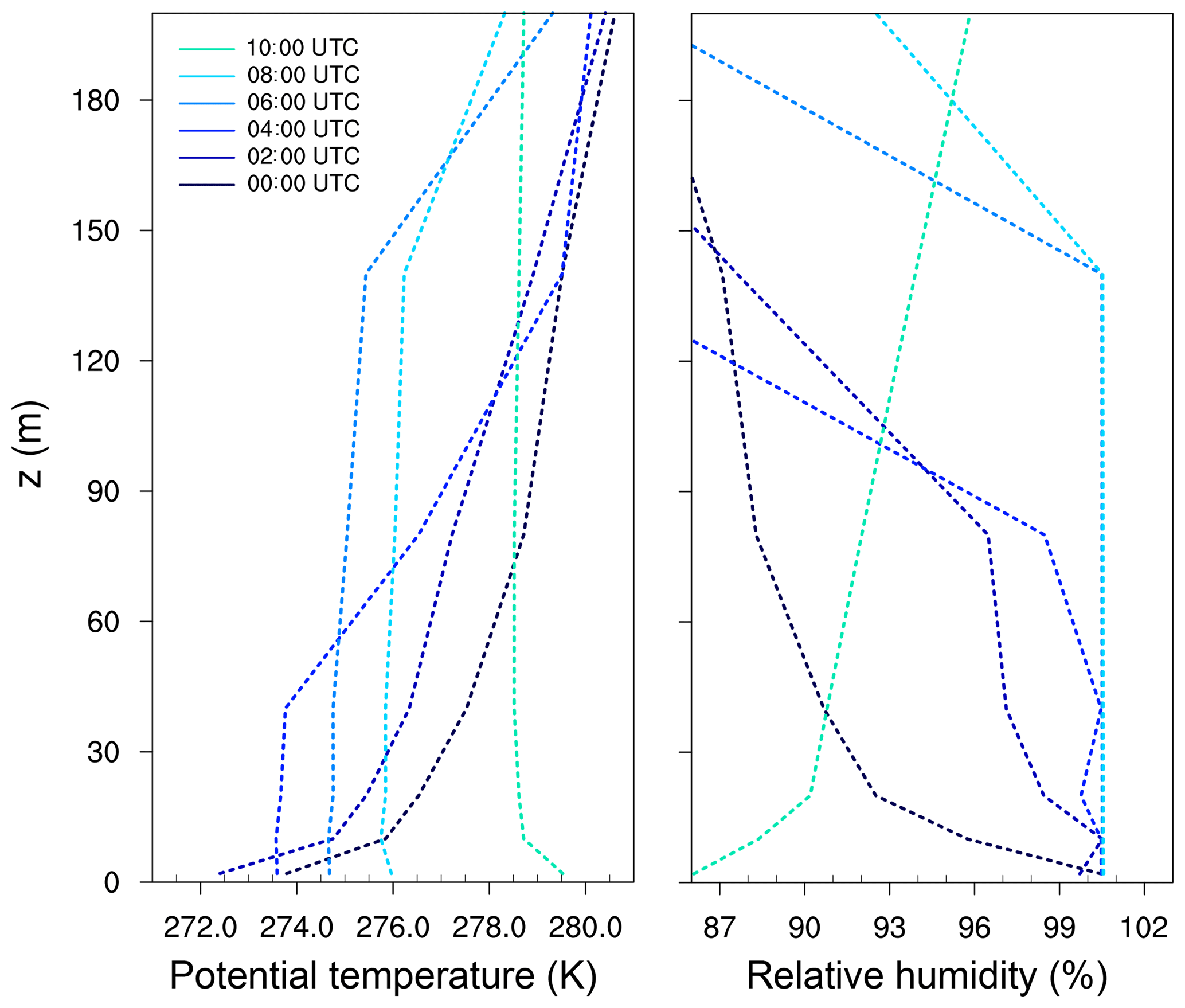
Figure 1Profiles of potential temperature and relative humidity at different times, as observed at Cabauw.
The model was initialized as described in the precursor study of Maronga and Bosveld (2017). Profiles of temperature and humidity (see Fig. 1) were derived from the CESAR 200 m tower and used as initial profiles in PALM. A geostrophic wind of 5.5 m s−1 was prescribed based on the observed value at Cabauw at 00:00 UTC.
The land surface model was initialized with short grassland as surface type and four soil model layers at the depths of 0.07, 0.28, 1.0 and 2.89 m. The measured surface layer temperatures were interpolated to the respective levels, resulting in temperatures of 279.54, 279.60, 279.16 and 279.16 K for soil layers one to four, respectively. Furthermore, the initial soil moisture was set to the value at field capacity (0.491 m3 m−3), which reflects the very wet soil and low water table in the Cabauw area. Moreover, the roughness length for momentum was prescribed to 0.15 m. Note that Maronga and Bosveld (2017) discussed that this value appears to be a little high given the season and wind direction. This does not play an important role in the present study, however, as we will not focus on direct comparison against observational data from Cabauw.
All simulations start at 00:00 UTC, before fog formation, and end at 10:15 UTC on the next morning after the fog layer has fully dissipated. Precursor runs are conducted for an additional 25 min using the initial state at 00:00 UTC, but without radiation scheme and LSM in order to allow the development of turbulence in the model without introducing feedback during that time (see Maronga and Bosveld, 2017).
Based on sensitivity studies of Maronga and Bosveld (2017), a grid spacing of Δ=1 m was adopted for all simulations, with a model domain size of grid points in x, y and z direction, respectively. Cyclic conditions were used at the lateral boundaries. A sponge layer was used starting at a height of 344 m in order to prevent gravity waves from being reflected at the top boundary of the model.
Table 1 gives an overview of the simulation cases. All cases were initialized with (identical) continental aerosol conditions. Case SAT represents a reference run with no activation scheme and thus a prescribed constant value of nc=150 cm−3 (estimated from simulations of Boers et al., 2013). This case represents the same setup to the one described in Maronga and Bosveld (2017) except for modifications concerning the aerosol environment as outlined below. Condensation processes were treated here with the saturation adjustment scheme (Seifert et al., 2006). In order to evaluate the influence of saturation adjustment in a one-moment microphysics scheme on the development of radiation fog, identical assumptions were made in case DIA and PRG, except that diffusional growth was calculated with the diagnostic and prognostic method, respectively (see Sect. 2.2.2).
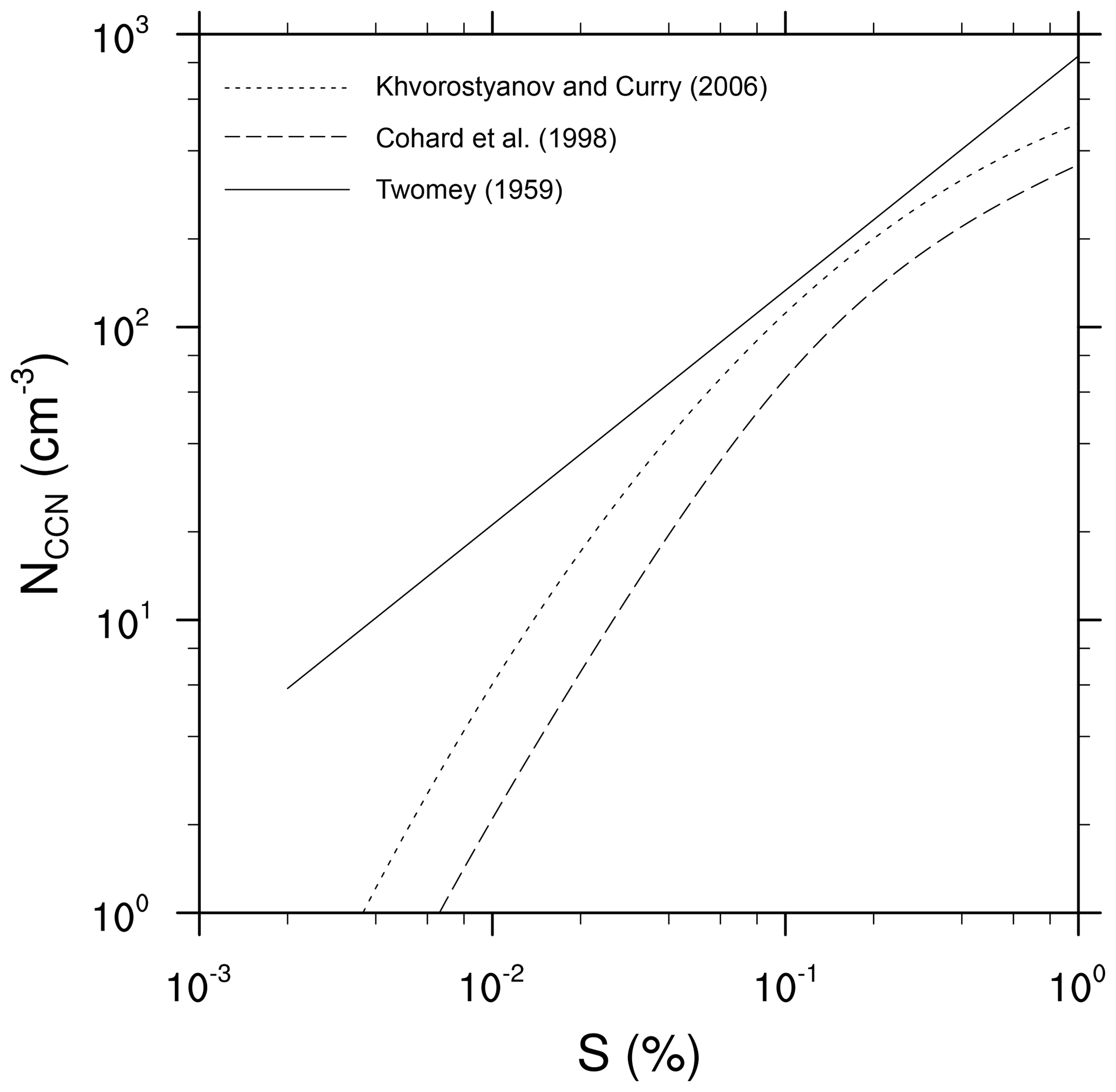
Figure 2Activation spectrum for three different activation schemes of Twomey (1959), Cohard et al. (1998), and Khvorostyanov and Curry (2006) for a typical continental aerosol environment.
Moreover, as small differences in supersaturation can affect the number of activated droplets significantly, the impact of different methods for calculating supersaturation on CCN activation is investigated in a two-moment microphysics approach (see Sect. 4.2.2). Therefore, the simulations N2SAT, N2DIA and N2PRG were compared to each other. In all three cases the activation scheme of Cohard et al. (1998) is used and initialized as described below.
Furthermore, cases N1DIA–N3DIA used the activation schemes described in Sect. 2.2.1. To ensure comparability between the different schemes, all of them were initialized with a continental aerosol background described in Cohard et al. (1998), which is characterized by an aerosol with the chemical composition of ammonium sulfate [(NH4)2SO4], a background aerosol concentration of 842 cm−3, a mean dry aerosol radius of rd0=0.0218 µm and a dispersion parameter of the dry aerosol spectrum of σd=3.19. For the Twomey activation scheme this results in N0=842 cm−3 and k=0.8, which is a typical value for the exponent for continental air masses (e.g., Pruppacher and Klett, 1997, p. 289 et seq.). The Twomey activation scheme does not allow for taking aerosol properties into account. In contrast, the activation scheme of Cohard et al. (1998) requires the parameters C, k, β and μ to be derived from the aerosol properties. Here, values of cm−3, k=3.251, β=621.689 and μ=2.589 were used as described in Cohard and Pinty (2000). Finally, the activation scheme of Khvorostyanov and Curry (2006) can directly consider the aerosol properties, which are prescribed as previously mentioned. Using those different parameterizations resulted in different activation spectra, which are shown in Fig. 2. One can see that especially the CCN concentration is changed by using these different methods, such that this part of the study is equivalent to a sensitivity study of different CCN concentration but is realized by using different coexisting parameterizations.
4.1 General fog life cycle and macrostructure
The reference case SAT is conducted with a constant droplet number concentration of nc=150 cm−3. The deepening of the fog layer can be seen in Fig. 3, which shows the profiles of the potential temperature, relative humidity and liquid water mixing ratio at different times.
The fog onset is at 00:55 UTC, defined by a visibility below 1000 m and a relative humidity of 100 %. In the following the fog layer deepens and extends to a top of approximately 20 m at 02:00 UTC. However, at this point the stratification of the layer is still stable with a temperature gradient of 6 K between the surface and the fog top. The persistent radiative cooling of the surface and the fog layer leads to a further vertical development of the fog, which is accompanied with a regime transition from stable to convective conditions within the fog layer (see Fig. 3a). This starts as soon as the fog layer begins to become optically thick (at 03:30 UTC), and when radiative cooling at the fog top becomes the dominant process, creating a top-down convective boundary layer. The highest liquid water mixing ratio of ql=0.41 g kg−1 is achieved at 06:00 UTC at a height of 60 m (see Fig. 3c), while the fog layer in total reaches the maximum 1 h later at 07:00 UTC. The lifting of the fog, which is defined by a non-cloudy near-surface layer (ql≤0.01 g kg−1), occurs at 08:45 UTC. At 11:30 UTC the fog is completely dissipated.
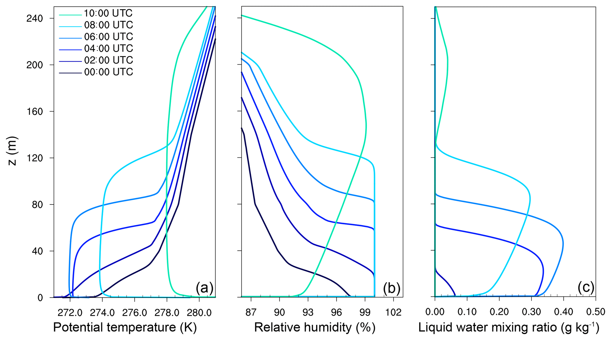
Figure 3Profiles of potential temperature (a), relative humidity (b) and liquid water mixing ratio (c) at different times for the reference case REF.
4.2 Influence of different supersaturation calculation
In this section we discuss the influence of three different method considering supersaturation. Namely these are (as previously mentioned) saturation adjustment, a diagnostic supersaturation calculation and a prognostic method. In the first subsection a one-moment microphysics scheme is used and the impact of the different supersaturation methods is limited to the effect of diffusional growth. In the second part of this study those methods are applied in a two-moment microphysics scheme, considering the effect of such different approaches of supersaturation calculations for activation.
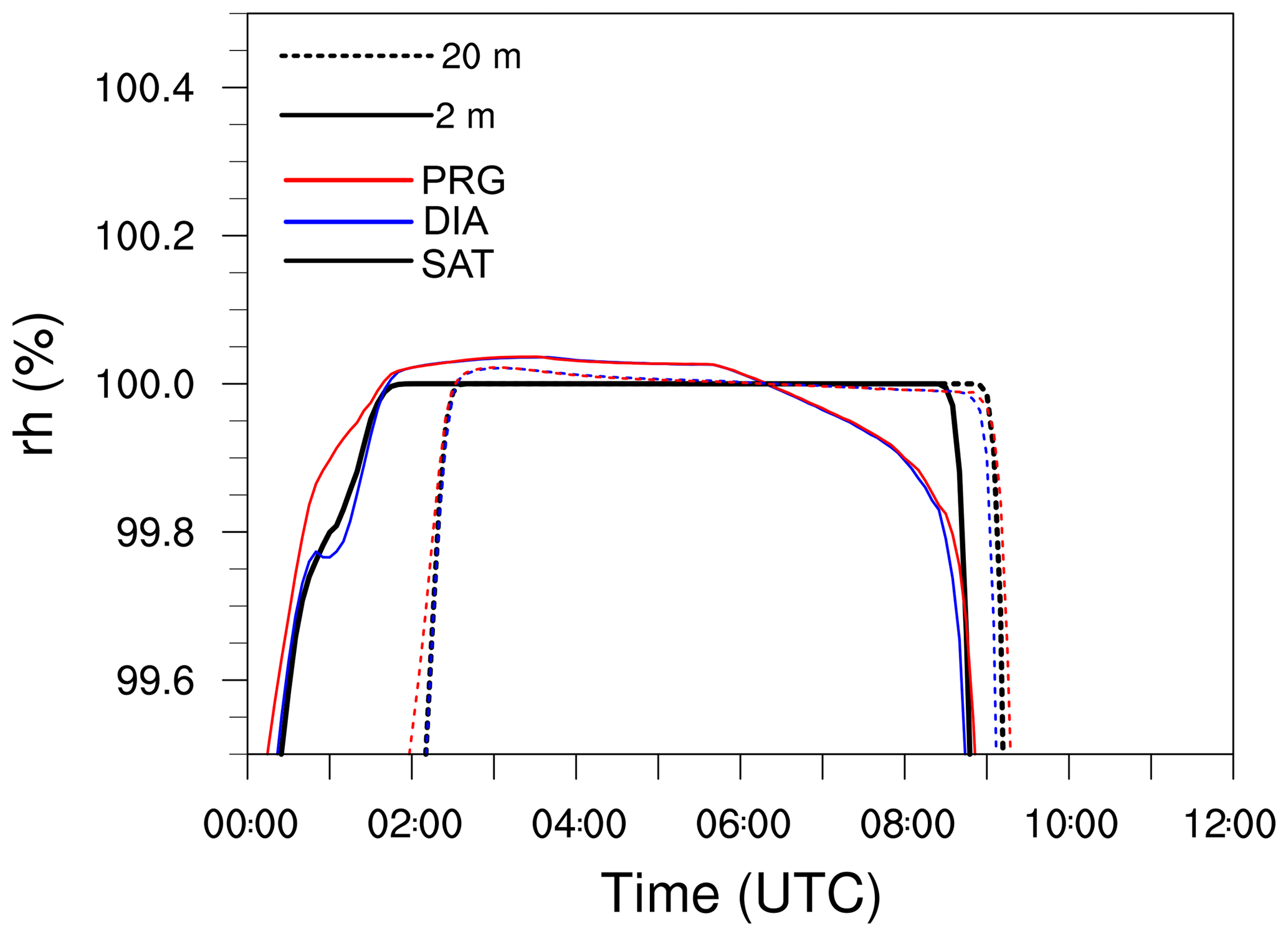
Figure 4Time series of horizontally averaged relative humidity (rh) and supersaturation at height levels of 2 m (solid) and 20 m (dotted) for different methods in treating the supersaturation calculation.
4.2.1 One-moment microphysics scheme: impact of supersaturation calculation on diffusional growth
In this section we discuss the error introduced by using saturation adjustment for simulating radiation fog with a one-moment scheme in a LES. For this, we compare three simulations with identical setups (cases SAT, DIA, and PRG), which differ only in the way supersaturation is calculated and consequently the amount of condensed or evaporated liquid water. To isolate this effect, activation is neglected in all cases and nc is set to a constant value of 150 cm−3 (a typical value in fog layers). The effect on different supersaturations driving the diabatic process of activation is discussed in Sect. 4.2.2. As mentioned before the time step is roughly 0.1 s, which is more than 1 order of magnitude smaller than the allowed values of 2–5 s for assuming saturation adjustment (Thouron et al., 2012). The present case hence is an ideal environment evaluating the error introduced by using saturation adjustment and by keeping all other parameters fixed.
Figure 4 shows time series of the horizontally averaged saturation (supersaturation) for cases SAT, DIA and PRG at selected heights close to the surface. In all cases saturation occurs simultaneously around 01:20 UTC. In case SAT, relative humidity does not exceed 100 % due to its limitation by saturation adjustment, while in case DIA and PRG, average supersaturations of 0.05 % are reached at a height of 2 m, which corresponds to typical values within fog (Hammer et al., 2014; Mazoyer et al., 2019; Boutle et al., 2018).
For cases DIA and PRG, starting from 06:15 UTC (in 2 m height) and 07:15 UTC (in 20 m height), supersaturations are removed and the air becomes subsaturated (on average). This is in contrast with case SAT, where the saturation adjustment approach keeps the relative humidity at 100 % as long as liquid water is present (i.e., until the fog has dissipated). Around 06:00 UTC, which is shortly after sunrise, relative humidity drops rapidly in PRG and DIA as a direct consequence of direct solar heating of the surface and the near-surface air, preventing further supersaturation at these heights. While we cannot clearly identify the lifting of the fog in case DIA and PRG (due to the limited humidity range displayed), we note that for case SAT we can identify lifting times as a decrease of relative humidity around 08:45 UTC at 2 m height and around 09:10 UTC at 20 m height.
Besides this inherent difference in relative humidity, the general time marks (formation, lifting and dissipation, defined by Maronga and Bosveld, 2017) of the fog layer are identical for cases SAT, DIA and PRG.
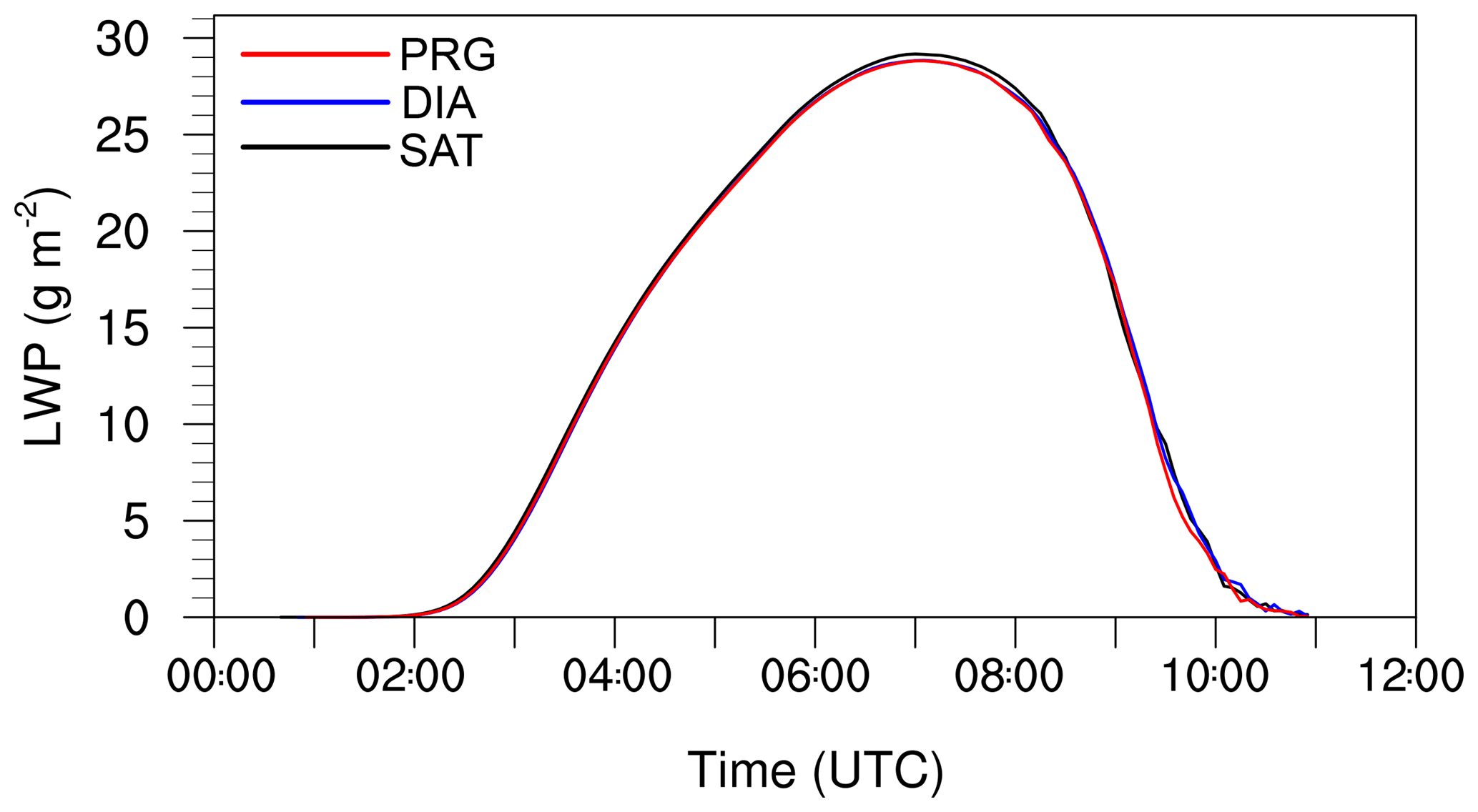
Figure 5Time series of liquid water path (LWP) for cases using saturation adjustment, the diagnostic approach and a prognostic method for the diffusional growth.
Figure 5 shows the liquid water path (LWP) for all cases. Differences in the LWP appear between 04:00 and 11:00 UTC and do not exceed 1 % (lower values for cases DIA and PRG), indicating that the choice of the condensation scheme does not affect the total water content of the simulated fog layer.
It can be summarized that, although the assumptions of saturation adjustment are not valid for the simulation of fog when using a very small time step, the mean liquid water content is not changed by more than 1 % and the general fog structure is not altered when using a one-moment microphysics and neglecting supersaturation. This is probably due to the very small supersaturation that is not strong enough to generate a significant change in the effective droplet radius and which could possibly lead to stronger sedimentation or higher radiative cooling rates.
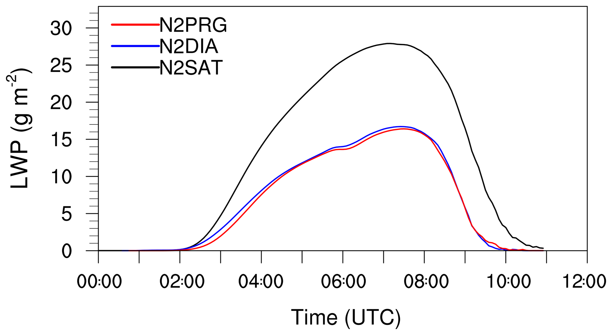
Figure 6Time series of LWP for simulations using saturation adjustment (N2SAT in black), the diagnostic scheme (N2DIA in blue) and the prognostic method (N2PRG in red). All cases use the activation scheme of Cohard et al. (1998).

Figure 7Profiles for liquid water mixing ratio (a) and droplet number concentration (b) at 04:00, 06:00 and 08:00 UTC.
4.2.2 Two-moment microphysics scheme: impact of supersaturation calculation on CCN activation
Even though different methods for calculating supersaturation which interacts with the diffusional growth are not strong enough to generate any noteworthy differences by using a one-moment microphysics (considering a constant value for nc), the impact of different methods modeling supersaturation on CCN activation by using a two-moment microphysics might be significant.
Cohard et al. (1998)Cohard et al. (1998)Cohard et al. (1998)Twomey (1959)Khvorostyanov and Curry (2006)Table 1Overview of conducted simulations. The droplet number concentration nc is only prescribed for simulations without activation scheme. In the simulations N1DIA–N3DIA, nc is a prognostic quantity and is thus variable in time and space. The aerosol background concentration is abbreviated with Na,tot and used to initialize the activation schemes. Note for the scheme after Cohard et al. (1998) a conversion to the parameter C must be applied, while for both other activation schemes this value is directly used to prescribe N0 and Nt, respectively.
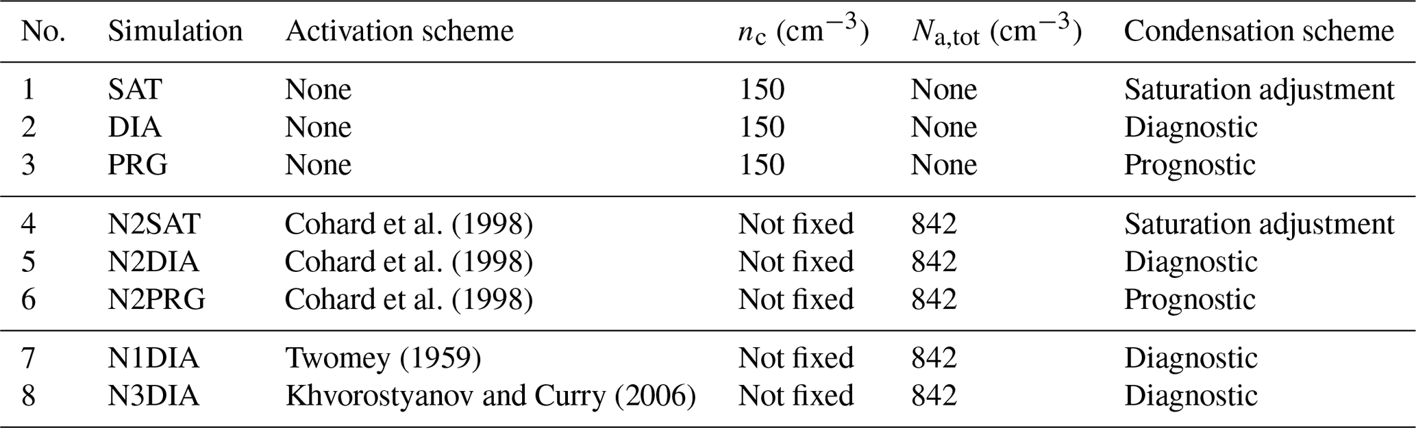
Figure 6 shows the LWP for simulations applying the activation scheme of Cohard et al. (1998) in conjunction with the usage of saturation adjustment (N2SAT), the diagnostic scheme (N2DIA) and the prognostic scheme (N2PRG) for calculating supersaturations. It can be seen that the prognostic and diagnostic methods produce similar LWP values. However, for case N2SAT the LWP is nearly 70 % higher than for the other two cases. In Fig. 7 profiles of the liquid water mixing ratio (left) and droplet number concentration (right) are shown. From that figure it can be seen that in case of N2SAT, both the fog height as well as the liquid water mixing ratios within the layer are higher than in N2DIA and N2PRG, respectively. However, small differences in ql can also be found between N2DIA and N2PRG (e.g., at 06:00 UTC in the second third of the fog layer). This is explained by slightly higher values for the number concentration in case of N2DIA than in N2PRG. However, both are at approximately 75 cm−3 at 06:00 UTC. In contrast, in simulation N2SAT, a number concentration of 120 to 150 cm−3 (at the top) is observed, which is about 60 %–100 % higher in comparison to N2DIA and N2PRG. These differences can be explained by the different methods for calculating the supersaturation, since activation is the main process altering the droplet number concentration. Therefore, we can implicitly derive from the droplet number concentration that the predicted and diagnosed supersaturations using the prognostic and diagnostic method are similar. These differences between N2SAT and N2DIA–N2PRG are, however, in good agreement with values reported for a stratocumulus case by Thouron et al. (2012). Their Fig. 2 shows that the number concentration of the diagnostic and prognostic method were also similar and the case with saturation adjustment overestimated the supersaturation and therefore the droplet number concentration. As the fog droplet number concentration has a crucial feedback on the overall LWP of the fog layer, the times of lifting and the time of its dissipation, the reported differences in nc are significant regarding the accurate modeling and prediction of fog. The reason why the number concentration is such a critically parameter can be ascribed to their impact on sedimentation and radiative cooling, which is explained in more detail in Sect. 4.4.3.

In order to evaluate the possible effect of the grid spacing, in conjunction with different methods for calculating the supersaturation, on CCN activation, we repeated each of the cases N2SAT, N2DIA and N2PRG with two coarser grid spacings of 2 and 4 m. The general effect of the grid spacing on the temporal development and structure of radiation fog is discussed in detail in Maronga and Bosveld (2017). In this section, we will focus only on changes in LWP due to different supersaturation calculations at different spatial model resolutions. For isolating the effect of the grid spacing, all simulations with a coarser grid spacing were carried out with the same time step of 0.125 s, which corresponds to the average time step of the simulations at highest grid spacing of 1 m. In this way, effects of different time steps induced by different grid spacings could be eliminated.
Figure 8 shows the LWP for all grid sensitivity runs. First of all, note that for 1 m grid spacing, the results reflect the results shown in Fig. 6 and discussed above (i.e., significantly higher LWP for case N2SAT than for cases N2DIA and N2PRG). Moreover, Fig. 8 reveals that these results are somewhat sensitive to changes in the grid spacing. For all cases we observe a tendency towards higher LWP values with increasing grid spacing, at least for cases N2DIA and N2PRG. These difference are, however, not larger than 4 g m−2 and are thus significantly smaller than the observed differences found between the different methods to calculate supersaturation. Note, however, that the relative change in LWP with grid spacing is higher for case N2DIA than for case N2PRG. Quantitatively speaking, in case of 1 m grid spacing the relative difference of the LWP is 2.1 % between N2DIA and N2PRG during the mature phase, while for the case with a grid spacing of 4 m it reaches 8.1 %. This might be explained by the fact that the diagnostic scheme is very sensitive to small errors (e.g., induced by the numerical advection) in the temperature and humidity fields (e.g., Morrison and Grabowski, 2008; Thouron et al., 2012). A coarser spatial resolution here can lead to larger error introduced by spurious supersaturation. We thus suppose that the increased differences (see Fig. 8) by larger grid spacings are induced by spurious supersaturation, which affect the CCN activation and hence influence the LWP of the fog layer.
Furthermore, we note that coarser grid spacings lead to a later fog formation time, which is in agreement with Maronga and Bosveld (2017) and can be ascribed to under-resolved turbulence near the surface at coarse grids.
In summary, we can thus conclude that the sensitivity to changes in the grid spacing is rather small, but it might imply differences in the LWP of the simulated fog layer of up to 4 g m−2.

Figure 9Time series of LWP and nc (as a horizontal and vertical average of the fog layer) for the reference and N1DIA–N3DIA case.
4.3 Two-moment microphysics scheme: comparison of different activation parameterizations
In numerous previous studies, the influence of aerosols and the activation process on the life cycle of fog was investigated (e.g., Bott, 1991; Stolaki et al., 2015; Maalick et al., 2016; Zhang et al., 2014; Boutle et al., 2018). Although all three activation schemes outlined in Sect. 2.2.1 are comparable power law parameterizations that are initialized with identical aerosol spectra, the effect on simulations of radiation fog is still unknown. Because changes in nc due to different activation schemes have a considerable effect on the life cycle of fog, we might consider that even small differences in nc might alter simulated fog layers significantly. This part of the study can be regarded as a sensitivity study of different CCN concentrations realized by applying different activation schemes, which is illustrated also in Fig. 2. However, from a model user's perspective, such a sensitivity is of great importance, as CCN concentrations are usually difficult (case studies) or even impossible (forecasting) to obtain, and model results thus might highly depend on the chosen activation parameterization.

4.4 LWP and nc
Time series of the LWP for the reference run (case SAT) and the three different cases (N1DIA–N3DIA) are shown in Fig. 9a. The highest LWP occurs for case SAT, which also shows the highest nc during the formation and mature phase in comparison with the other simulations (see Fig. 9b). The time series of nc shown in Fig. 9b (representing runs with the three different aerosol activation parameterization schemes; see Table 1) reveal that, depending on the parameterization used, the a shift in nc towards smaller or larger values is found. The quantitative differences in the number of activated aerosol by using the different activation schemes is due to a slightly different activation spectrum (see Fig. 2). A linear relationship between LWP and nc can be found: a higher nc leads to higher LWP, which is in agreement with other studies, like Boutle et al. (2018), for example. In principle, a similar qualitative development of nc can be observed. While nc increases during fog formation (with a local maximum with values between 70 and 140 cm−3), it remains nearly constant during the mature phase of the fog (values between 65 and 145 cm−3). We will see later see that activation here happens mostly at the top of the fog, but due to vertical mixing in the convective fog layer, cloud droplets are evenly distributed over a large vertical domain. Furthermore, the mixing layer is increasing in time so that there is no net change of the (averaged) nc in the fog layer. As soon as the sun rises and the fog layers start to lift and turn into a stratocumulus cloud, all cases show a strong increase in nc. This increase can be explained by stronger supersaturations induced by thermal updrafts in the developing surface-driven convective boundary layer due to surface heating by solar radiation. Moreover, we note that while the qualitative course of nc is similar for all cases, the choice of the activation algorithm has an impact on the number of activated aerosols and thus on the strength of the fog layer, e.g., illustrated in Fig. 10 via ql. This is due to the radiation effect of the droplets. The number of droplets to which a certain amount of liquid water is distributed plays an important role: the larger the number of droplets, the larger the radiation–effective surface and the higher also the optical thickness. As a result the cooling rate in fog with many small droplets is increased, allowing more water vapor to condense and the fog to grow stronger. By the same token, sedimentation also depends on the droplet radius and plays a major role in fog development. This will be further discussed below.
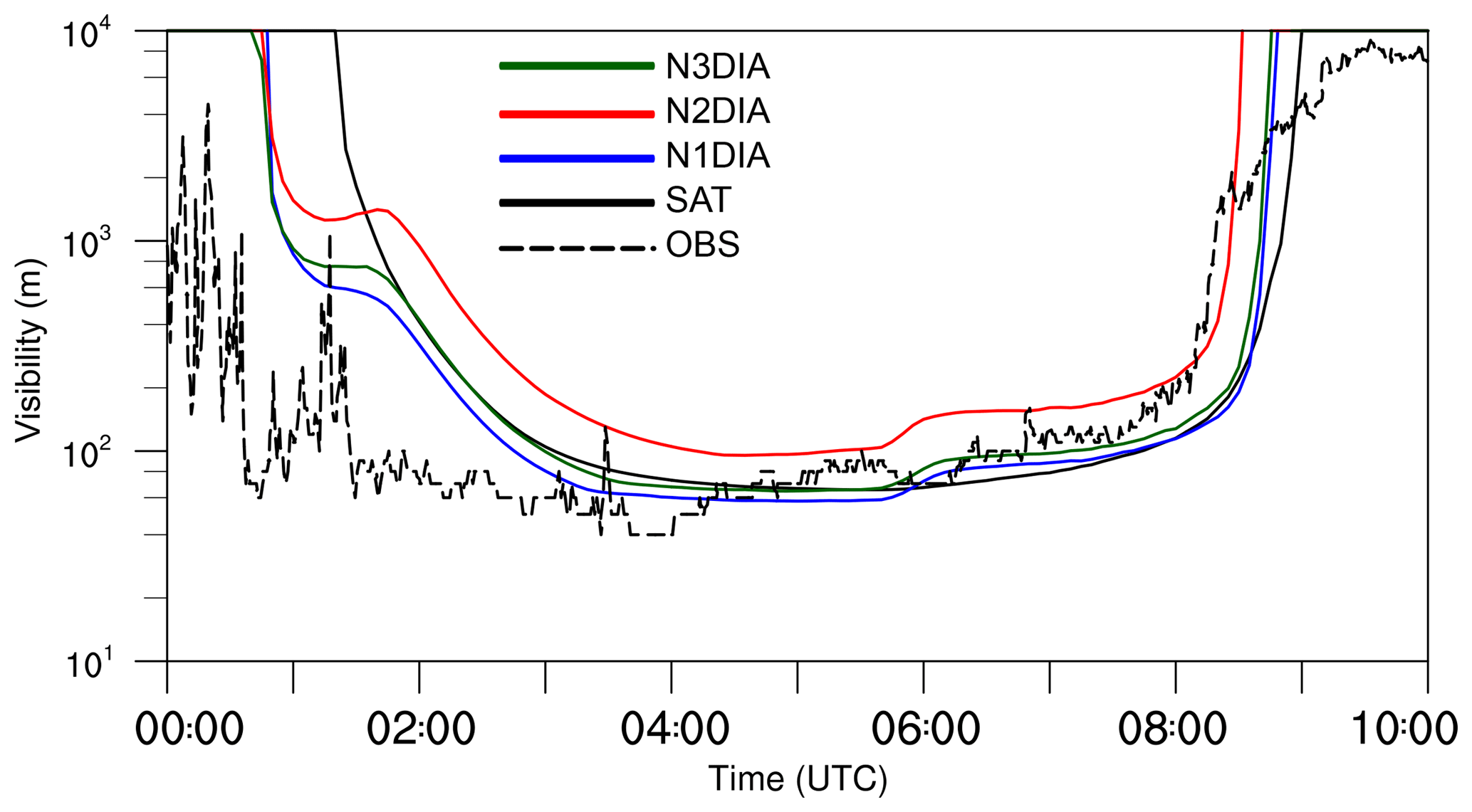
Figure 11Time series of simulated visibility in 2 m height. Observations from Cabauw (dashed lines) were added for illustration only.
4.4.1 Visibility
In Fig. 11 the simulated visibility is shown for the cases N1DIA–N3DIA in 2 m height together with the observed values at Cabauw (for illustration only). Visibility is calculated from the LES data following Gultepe et al. (2006) as
This visibility estimation (with nc and ql given in units of cm−3 and g m−3, respectively) thus significantly depends on the droplet number concentration and the liquid water content. Unlike in the first part of this paper, analyzing visibility estimations from the simulations might illuminate the capability of LES to predict visibility. Figure 11 reveals that visibility follows the same general temporal developed for all cases, with a rapid decrease at fog formation, deepening and dissipation, with minimum values at around 100 m (which is close to the observed values). We also see noteworthy differences, particularly shortly before 02:00 UTC (before fog deepening) at around 05:45 UTC (shortly after sunrise). For both time marks, cases N1DIA–N3DIA display sudden increases in visibility, due to an fast decrease in nc in 2 m height, which are not reproduced by case SAT, as nc is fixed value in this case. The sudden increase in visibility around 00:45 UTC in the observations is possibly related to this process. Also, the time marks of formation and dissipation vary. For cases N1DIA–N3DIA, the formation time is significantly advanced compared to case SAT, while dissipation time only shows a small tendency towards earlier times, at least for N1DIA and N3DIA. Case N2DIA displays a different behavior, with a later fog formation and higher visibility and accordingly earlier dissipation time. This is in line with the findings discussed above (i.e., a much weaker fog layer that, as a direct consequence, can dissipate much faster). Otherwise, all cases display almost identical visibility as soon as the fog has deepened.
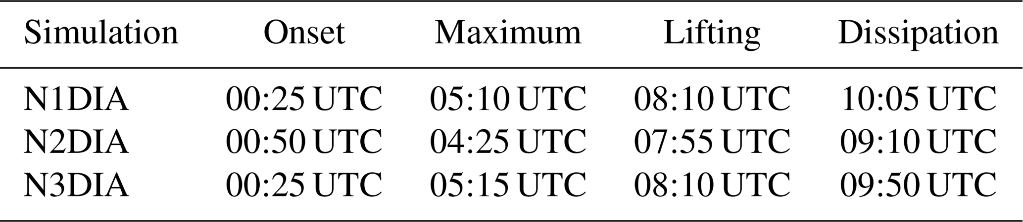
4.4.2 Time marks of the fog life cycle
The effect of the different droplet concentration (induced by the usage of different activation schemes) on the time marks of the fog life cycle is summarized in Table 2. While N1DIA and N3DIA have similar time marks, N2DIA stands out and shows a delayed onset by 25 min, while the maximum liquid water mixing ratio is reached 45 min earlier than in the other cases. Also lifting and dissipation are affected and occurred 15 and 40 min (with respect to simulation N3DIA) earlier. This is due to a lesser absolute liquid water mixing ratio which evaporates faster by the incoming solar radiation. Therefore, it can be concluded that the use of different activation schemes (if they change the droplet number concentration) has an effect on the time marks on the life cycle as well as on the fog height and the amount of liquid water within the fog layer.
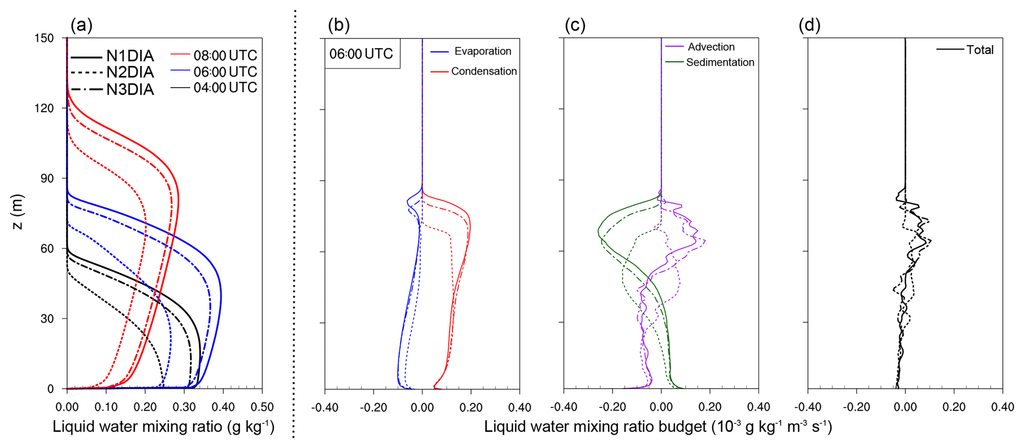
Figure 12Profiles (instantaneously and horizontally averaged) of liquid water mixing ratio at 04:00, 06:00 and 08:00 UTC, and profiles of liquid water budget terms at 06:00 UTC.
4.4.3 Budgets of liquid water and droplet number concentration
In this section we will analyze the budgets of liquid water and droplet number concentration in physical terms. As in the preceding section, we will use the cases with different activation parameterizations, since they provide us a range of different CCN concentrations. Figure 12a shows the profiles of the liquid water mixing ratio at 04:00, 06:00 and 08:00 UTC, i.e at different times during the mature phase of the fog. A detailed analysis of budgets at other stages of the life cycle of the fog is beyond the scope of this paper. The maximum ql in the fog layer is reached at approximately 06:00 UTC at a height of 60 m. Afterwards a further vertical growth of the fog can be observed, where no further increase in liquid water takes places as a result of larger vertical extent of the mixing layer and due to rising temperatures after sunrise. Moreover, Fig. 12b and c show the liquid water budget during the mature phase of the fog at 06:00 UTC, when the fog was fully developed. Almost all three cases show identical values for condensation rates in the lowest part of the fog layer, with values being in the same order as the evaporation rates so that the net gain in this region appears to be small (see Fig. 12b). However, the N2DIA case (with the lowest nc) exhibits a generally lower absolute evaporation rate compared to both other cases, which can be attributed to the slightly higher mean values of the relative humidity (not shown) than in N1DIA and N3DIA. In the upper part of the fog layer, higher values of the condensation rate are observed (especially for N1DIA and N3DIA) with a concurrent decrease in evaporation rates, leading to differently strong deepening of the fog layer. At a height of approximately 80 m, a maximum of the evaporation rates can be observed, representing the presence of subsaturated regions at this height and the top of the fog. Larger differences can be observed in the sedimentation rates. First and foremost the sedimentation is proportional to the liquid water mixing ratio (see also Eq. 4). The strength of sedimentation also depends on the mean radius of the droplets, which increases with a decreasing number of activated drops. Here, a lower nc for a given amount of liquid water leads to a higher mean radius, compared to a higher nc where the same amount of water is distributed to more drops, decreasing the mean radius. Integrated over height, all three cases exhibit approximately the same sedimentation rates. Therefore, case N2DIA experiences the strongest loss of liquid water due to sedimentation (in relative terms). Moreover, Fig. 12c shows that sedimentation partially counteracts the gains caused by condensation at the upper edge of the fog. The net advection transports liquid water from the second third of the fog layer (position of the maximum) to higher levels. It can be summarized that all terms contribute significantly to the net change of the liquid water mixing ratio, illustrating that all microphysical processes deserve a proper modeling for radiation fog. In the mature phase, however, sedimentation plays a key role, showing the highest values for the individual tendencies. As a result liquid water is slowly and constantly removed from the fog layer. These findings are in good agreement with previous investigations by Bott (1991).
The sum of all tendencies, which is shown in Fig. 12d, is the height-dependent change of the liquid water. Also here it can be seen that in the lower 50 m the net tendency is negative, while in higher levels we observe a positive tendency so that the fog continues growing vertically while the liquid water content within the fog layer decreases.
Figure 13a additionally shows the profiles of nc. We note that the profiles of the different cases differ quantitatively but not qualitatively. The stage of the fog can thus be identified in the profiles for all cases. At 04:00 UTC, the highest supersaturations occur close to the ground due to cooling of the surface and near-surface air, leading to high activation rates and therefore high nc near the surface (not shown). At 06:00 UTC a well-mixed layer has developed that is driven by the radiative cooling from the fog top. While the turbulent mixing leads to a vertical well-mixed nc, we note the maximum at the top, where the radiative cooling induces immense aerosol activation. This is further illustrated in the budget of the nc in Fig. 13b and c, where instantaneous data at 06:00 UTC are shown. Here, we see clearly that aerosol activation at the top of the fog layer is the dominant process in the mature phase of the fog, while activation near the surface is comparably small. Evaporation of droplets, though small in magnitude, occurs only at the fog top, reflecting upward motions of foggy air penetrating the subsaturated air aloft where droplets then evaporate. Also, we see that both advection and sedimentation rates are much smaller than activation rates so that the net change in nc is controlled by the activation near the fog top during the mature phase of the fog.
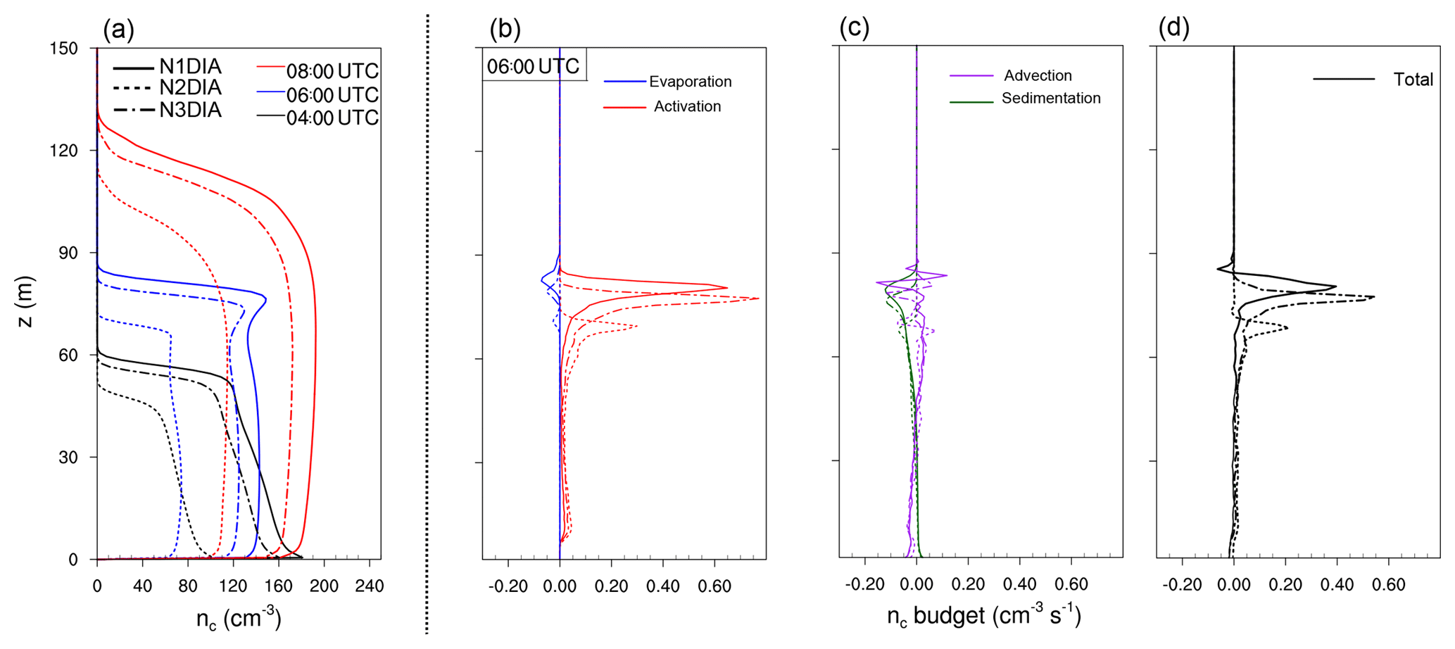
Figure 13Profiles (instantaneously and horizontally averaged) of nc at 04:00, 06:00 and 08:00 UTC, and profiles of nc budget terms at 06:00 UTC.
The main objective of this work was to investigate the influence of the choice of the supersaturation calculation and activation parameterizations used in LES models on the life cycle of simulated nocturnal deep radiation fog under typical continental aerosol conditions. For this purpose we performed a series of LES runs based on a typical deep fog event as observed at Cabauw (the Netherlands).
In the main part of this study we applied a two-moment microphysics scheme with an activation parameterization of Cohard et al. (1998) and investigated the influence of three different (but commonly used) supersaturation calculation methods, i.e., saturation adjustment, a diagnostic method, and a prognostic method, on the life cycle and LWP of the simulated fog event. From the results we found that in the case of saturation adjustment, nearly 60 % higher droplet number concentrations are produced in comparison with simulation with the diagnostic or prognostic method. This results in a more than 70 % higher LWP for the saturation adjustment case and a later occurrence of lifting and dissipation of the fog layer. An explanation for such differences between the schemes can be found in the general assumptions made within the methods. As saturation adjustment assumes that the complete water vapor surplus is removed within one time step, the supersaturation used for activation must be parameterized. In agreement with Thouron et al. (2012) we found that those values are higher than in the other cases, which leads to great feedback of the fog layer. Moreover, we found that the diagnostic method and the prognostic method yield similar results. However, in a grid spacing sensitivity study we observed that the relative differences between the prognostic and diagnostic approach increase as the spatial resolution decreases. We assume that this is due to larger errors of spurious supersaturations which lead to an overestimation of activation in the diagnostic case. This in turn affects the sedimentation velocity as well as the effective radius and hence the radiative cooling, which results in higher values for the LWP.
In a further test, using a one-moment microphysics scheme, we compared the possible error introduced by using saturation adjustment in comparison with an diagnostic and prognostic method for calculating the supersaturation for diffusional growth, i.e., neglecting activation and prescribing a constant droplet number concentration. With these assumptions we were able to isolate the error introduced by saturation adjustment on condensation and evaporation. However, the results showed that, although the model time step was inappropriate for the assumptions made during saturation adjustment, the differences in LWP are at most 1 % and the general life cycle is not affected. This could be attributed to the fact that the typical supersaturations in fog are in the range of a few tenths of a percent, and the resulting absolute differences are too small to induce further influence on dynamics, microphysics or radiation. This result implies that saturation adjustment is an acceptable method if no activation parameterization is available (with simultaneous consideration that the latter is highly recommended).
In a second part of our study, the effect of different activation schemes of Twomey (1959), Cohard et al. (1998), and Khvorostyanov and Curry (2006) on the simulated fog life cycle was investigated. Even though these parameterizations appear to be rather similar, our results indicate that the resulting number of activated aerosols (and consequently the number of droplets), known to be a crucial parameter for the fog development, can differ significantly. However, it must be mentioned that these differences are attributed to the fact that the CCN concentration is different for the investigated schemes. This part of the study can thus also be understood as a sensitivity study for different CCN concentrations realized by the usage of different activation schemes.
In order to get a deeper insight into the spatial and temporal development of deep radiation fog, we performed an additional analysis of budgets nc and ql during the mature phase of the fog for simulations with different aerosol activation parameterizations. We found that gain of liquid water is dominated by condensational growth throughout the fog layer with a maximum at the top of the fog layer (due to longwave radiative cooling) and by significant sedimentation of fog droplets from upper levels towards lower levels, while only little liquid water is lost by sedimentation (to the ground) and evaporation. The fact that the simulated cases display significant differences in the fog strength could be traced back to the differences in the condensational growth at the fog top, induced by different activation of CCN. For nc, our simulations indeed indicate that activation is the dominant process, located in a narrow height level, while all other processes (i.e., evaporation, advection and sedimentation) were found to be comparably small. The amount of generated liquid water thus is a direct consequence of the strength of the activation process and is thus related to the number of CCN and accordingly the activation parameterization used in the model.
In summary, the present study indicates that the choice of the used supersaturation calculation can be a key factor for the simulation of radiation fog. In agreement with Thouron et al. (2012) we recommend using the prognostic approach to calculate the supersaturation for fog layer in case of a two-moment microphysics considering activation. With this, the effect of spurious cloud-edge supersaturation is mitigated and activation rates that are too large are omitted. Further, the choice of the chosen activation scheme has a noticeable impact on the number concentration of CCN and hence on the LWP and fog layer depth. However, we have no means to give advice on which activation parameterization performs best. In order to give a more educated recommendation here, we would need observational data of size distributions from aerosol and fog droplets.
In order to overcome the remaining limitations of the present study that are related to microphysical parameterizations, we are currently working on a follow-up study in which we are revisiting this particular fog case using a Lagrangian particle-based approach to simulate the microphysics of droplets. This will allow for explicitly simulating the development of the 3-D droplet size distribution in the fog layer (e.g., Shima et al., 2009). This approach will also allow resolving all relevant microphysical processes such as activation and diffusional growth directly instead of parameterizing them. As such simulations are computationally very expensive, only a very limited number of simulations are feasible at the moment, so most future numerical investigations will – as in the present work – rely on bulk microphysics parameterizations. Based on the results using the Lagrangian approach, however, we hope to be able to give an educated recommendation on the best choice for such bulk parameterizations.
The PALM used in this study (revision 2675 and revision 3622) is publicly available on http://palm-model.org/trac/browser/palm?rev=2675 (last access: 28 May 2019) (PALM, 2019a) and http://palm-model.org/trac/browser/palm?rev=3622 (last access: 28 May 2019) (PALM, 2019b), respectively. For analysis, the model has been extended and additional analysis tools have been developed. The extended code, as well as the job setups and the PALM source code used, are publicly available on https://doi.org/10.25835/0067929 (PALM group, 2019c). All questions concerning the code-extension will be answered from the authors on request.
The numerical experiments were jointly designed by the authors. JS implemented the microphysics parameterizations, conducted the simulations and performed the data analysis. Results were jointly discussed. JS prepared the paper, with significant contributions by BM.
The authors declare that they have no conflict of interest.
This work has been funded by the German Research Foundation (DFG) under grant MA 6383/1-1, which is greatly acknowledged. All simulations have been carried out on the Cray XC-40 systems of the North-German Supercomputing Alliance (HLRN; https://www.hlrn.de/, last access: 28 May 2019).
This research has been supported by the German Research Foundation (grant no. MA 6383/1-1).
The publication of this article was funded by the
open-access fund of Leibniz Universität Hannover.
This paper was edited by Barbara Ervens and reviewed by Thierry Bergot and one anonymous referee.
Abdul-Razzak, H. and Ghan, S. J.: A parameterization of aerosol activation: 2. Multiple aerosol types, J. Geophys. Res.-Atmos., 105, 6837–6844, 2000. a
Ackerman, A. S., VanZanten, M. C., Stevens, B., Savic-Jovcic, V., Bretherton, C. S., Chlond, A., Golaz, J.-C., Jiang, H., Khairoutdinov, M., Krueger, S. K., Lewellen, D. C., Lock, A., Moeng, C.-H., Nakamura, K., Petters, M. D., Snider, J. R., Weinbrecht, S., and Zulauf, M.: Large-eddy simulations of a drizzling, stratocumulus-topped marine boundary layer, Mon. Weather Rev., 137, 1083–1110, 2009. a
Árnason, G. and Brown Jr., P. S.: Growth of cloud droplets by condensation: A problem in computational stability, J. Atmos. Sci., 28, 72–77, 1971. a
Beare, R. J., Macvean, M. K., Holtslag, A. A., Cuxart, J., Esau, I., Golaz, J.-C., Jimenez, M. A., Khairoutdinov, M., Kosovic, B., Lewellen, D., Lund, T. S., Lundquist, J. K., Mccabe, A., Moene, A. F., Noh, Y., Raasch, S., and Sullivan, P.: An intercomparison of large-eddy simulations of the stable boundary layer, Bound.-Lay. Meteorol., 118, 247–272, 2006. a
Bergot, T.: Small-scale structure of radiation fog: a large-eddy simulation study, Q. J. Roy. Meteorol. Soc., 139, 1099–1112, 2013. a
Boers, R., Baltink, H. K., Hemink, H., Bosveld, F., and Moerman, M.: Ground-based observations and modeling of the visibility and radar reflectivity in a radiation fog layer, J. Atmos. Ocean. Tech., 30, 288–300, 2013. a, b, c
Bott, A.: On the influence of the physico-chemical properties of aerosols on the life cycle of radiation fogs, Bound.-Lay. Meteorol., 56, 1–31, 1991. a, b, c
Bott, A. and Trautmann, T.: PAFOG – a new efficient forecast model of radiation fog and low-level stratiform clouds, Atmos. Res., 64, 191–203, 2002. a, b
Bougeault, P.: Modeling the trade-wind cumulus boundary layer. Part I: Testing the ensemble cloud relations against numerical data, J. Atmos. Sci., 38, 2414–2428, 1981. a
Boutle, I., Price, J., Kudzotsa, I., Kokkola, H., and Romakkaniemi, S.: Aerosol-fog interaction and the transition to well-mixed radiation fog, Atmos. Chem. Phys., 18, 7827–7840, https://doi.org/10.5194/acp-18-7827-2018, 2018. a, b, c, d, e, f
Clark, T. L.: Numerical modeling of the dynamics and microphysics of warm cumulus convection, J. Atmos. Sci., 30, 857–878, 1973. a, b
Clough, S. A., Shephard, M. W., Mlawer, E. J., Delamere, J. S., Iacono, M. J., Cady-Pereira, K., Boukabara, S., and Brown, P. D.: Atmospheric radiative transfer modeling: A summary of the AER codes, Short Communication, J. Quant. Spectrosc. Ra., 91, 233–244, 2005. a
Cohard, J.-M. and Pinty, J.-P.: A comprehensive two-moment warm microphysical bulk scheme. I: Description and tests, Q. J. Roy. Meteorol. Soc., 126, 1815–1842, 2000. a, b
Cohard, J.-M., Pinty, J.-P., and Bedos, C.: Extending Twomey's analytical estimate of nucleated cloud droplet concentrations from CCN spectra, J. Atmos. Sci., 55, 3348–3357, 1998. a, b, c, d, e, f, g, h, i, j, k, l, m, n, o, p, q, r, s
Cohard, J.-M., Pinty, J.-P., and Suhre, K.: On the parameterization of activation spectra from cloud condensation nuclei microphysical properties, J. Geophys. Res.-Atmos., 105, 11753–11766, 2000. a
Deardorff, J. W.: Stratocumulus-capped mixed layers derived from a three-dimensional model, Bound.-Lay. Meteorol., 18, 495–527, 1980. a
Geoffroy, O., Brenguier, J.-L., and Sandu, I.: Relationship between drizzle rate, liquid water path and droplet concentration at the scale of a stratocumulus cloud system, Atmos. Chem. Phys., 8, 4641–4654, https://doi.org/10.5194/acp-8-4641-2008, 2008. a
Geoffroy, O., Brenguier, J.-L., and Burnet, F.: Parametric representation of the cloud droplet spectra for LES warm bulk microphysical schemes, Atmos. Chem. Phys., 10, 4835–4848, https://doi.org/10.5194/acp-10-4835-2010, 2010. a
Grabowski, W. W. and Morrison, H.: Toward the mitigation of spurious cloud-edge supersaturation in cloud models, Mon. Weather Rev., 136, 1224–1234, 2008. a
Gultepe, I., Müller, M. D., and Boybeyi, Z.: A new visibility parameterization for warm-fog applications in numerical weather prediction models, J. Appl. Meteor. Climatol., 45, 1469–1480, 2006. a
Gultepe, I., Tardif, R., Michaelides, S., Cermak, J., Bott, A., Bendix, J., Müller, M. D., Pagowski, M., Hansen, B., Ellrod, G., Jacobs, W., Toth, G., and Cober, S. G.: Fog research: A review of past achievements and future perspectives, in: Fog and Boundary Layer Clouds: Fog Visibility and Forecasting, Springer, 1121–1159, 2007. a, b
Gultepe, I., Hansen, B., Cober, S., Pearson, G., Milbrandt, J., Platnick, S., Taylor, P., Gordon, M., and Oakley, J.: The fog remote sensing and modeling field project, B. Am. Meteorol. Soc., 90, 341–359, 2009. a
Haeffelin, M., Bergot, T., Elias, T., Tardif, R., Carrer, D., Chazette, P., Colomb, M., Drobinski, P., Dupont, E., Dupont, J.-C., Gomes, L., Musson-Genon, L., Pietras, C., Plana-Fattori, A., Protat, A., Rangognio, J., Raut, J.-C., Rémy, S., Richard, D., Sciare, J., and Zhang, X.: PARISFOG: shedding new light on fog physical processes, B. Am. Meteorol. Soc., 91, 767–783, 2010. a
Hammer, E., Gysel, M., Roberts, G. C., Elias, T., Hofer, J., Hoyle, C. R., Bukowiecki, N., Dupont, J.-C., Burnet, F., Baltensperger, U., and Weingartner, E.: Size-dependent particle activation properties in fog during the ParisFog 2012/13 field campaign, Atmos. Chem. Phys., 14, 10517–10533, https://doi.org/10.5194/acp-14-10517-2014, 2014. a, b
Heus, T., van Heerwaarden, C. C., Jonker, H. J. J., Pier Siebesma, A., Axelsen, S., van den Dries, K., Geoffroy, O., Moene, A. F., Pino, D., de Roode, S. R., and Vilà-Guerau de Arellano, J.: Formulation of the Dutch Atmospheric Large-Eddy Simulation (DALES) and overview of its applications, Geosci. Model Dev., 3, 415–444, https://doi.org/10.5194/gmd-3-415-2010, 2010. a
Khairoutdinov, M. and Kogan, Y.: A new cloud physics parameterization in a large-eddy simulation model of marine stratocumulus, Mon. Weather Rev., 128, 229–243, 2000. a, b, c
Khvorostyanov, V. I. and Curry, J. A.: Aerosol size spectra and CCN activity spectra: Reconciling the lognormal, algebraic, and power laws, J. Geophys. Res.-Atmos., 111, D12202, https://doi.org/10.1029/2005JD006532, 2006. a, b, c, d, e, f
Kokkola, H., Korhonen, H., Lehtinen, K. E. J., Makkonen, R., Asmi, A., Järvenoja, S., Anttila, T., Partanen, A.-I., Kulmala, M., Järvinen, H., Laaksonen, A., and Kerminen, V.-M.: SALSA – a Sectional Aerosol module for Large Scale Applications, Atmos. Chem. Phys., 8, 2469–2483, https://doi.org/10.5194/acp-8-2469-2008, 2008. a
Lac, C., Chaboureau, J.-P., Masson, V., Pinty, J.-P., Tulet, P., Escobar, J., Leriche, M., Barthe, C., Aouizerats, B., Augros, C., Aumond, P., Auguste, F., Bechtold, P., Berthet, S., Bielli, S., Bosseur, F., Caumont, O., Cohard, J.-M., Colin, J., Couvreux, F., Cuxart, J., Delautier, G., Dauhut, T., Ducrocq, V., Filippi, J.-B., Gazen, D., Geoffroy, O., Gheusi, F., Honnert, R., Lafore, J.-P., Lebeaupin Brossier, C., Libois, Q., Lunet, T., Mari, C., Maric, T., Mascart, P., Mogé, M., Molinié, G., Nuissier, O., Pantillon, F., Peyrillé, P., Pergaud, J., Perraud, E., Pianezze, J., Redelsperger, J.-L., Ricard, D., Richard, E., Riette, S., Rodier, Q., Schoetter, R., Seyfried, L., Stein, J., Suhre, K., Taufour, M., Thouron, O., Turner, S., Verrelle, A., Vié, B., Visentin, F., Vionnet, V., and Wautelet, P.: Overview of the Meso-NH model version 5.4 and its applications, Geosci. Model Dev., 11, 1929–1969, https://doi.org/10.5194/gmd-11-1929-2018, 2018. a
Lebo, Z. J., Morrison, H., and Seinfeld, J. H.: Are simulated aerosol-induced effects on deep convective clouds strongly dependent on saturation adjustment?, Atmos. Chem. Phys., 12, 9941–9964, https://doi.org/10.5194/acp-12-9941-2012, 2012. a, b, c
Maalick, Z., Kühn, T., Korhonen, H., Kokkola, H., Laaksonen, A., and Romakkaniemi, S.: Effect of aerosol concentration and absorbing aerosol on the radiation fog life cycle, Atmos. Environ., 133, 26–33, 2016. a, b
Maronga, B. and Bosveld, F.: Key parameters for the life cycle of nocturnal radiation fog: a comprehensive large-eddy simulation study, Q. J. Roy. Meteor. Soc., 143, 2463–2480, 2017. a, b, c, d, e, f, g, h, i, j, k, l, m
Maronga, B., Gryschka, M., Heinze, R., Hoffmann, F., Kanani-Sühring, F., Keck, M., Ketelsen, K., Letzel, M. O., Sühring, M., and Raasch, S.: The Parallelized Large-Eddy Simulation Model (PALM) version 4.0 for atmospheric and oceanic flows: model formulation, recent developments, and future perspectives, Geosci. Model Dev., 8, 2515–2551, https://doi.org/10.5194/gmd-8-2515-2015, 2015. a, b
Mazoyer, M., Lac, C., Thouron, O., Bergot, T., Masson, V., and Musson-Genon, L.: Large eddy simulation of radiation fog: impact of dynamics on the fog life cycle, Atmos. Chem. Phys., 17, 13017–13035, https://doi.org/10.5194/acp-17-13017-2017, 2017. a, b, c, d
Mazoyer, M., Burnet, F., Denjean, C., Roberts, G. C., Haeffelin, M., Dupont, J.-C., and Elias, T.: Experimental study of the aerosol impact on fog microphysics, Atmos. Chem. Phys., 19, 4323–4344, https://doi.org/10.5194/acp-19-4323-2019, 2019. a
Mensah, A. A., Holzinger, R., Otjes, R., Trimborn, A., Mentel, Th. F., ten Brink, H., Henzing, B., and Kiendler-Scharr, A.: Aerosol chemical composition at Cabauw, The Netherlands as observed in two intensive periods in May 2008 and March 2009, Atmos. Chem. Phys., 12, 4723–4742, https://doi.org/10.5194/acp-12-4723-2012, 2012. a
Morrison, H. and Grabowski, W. W.: Comparison of bulk and bin warm-rain microphysics models using a kinematic framework, J. Atmos. Sci., 64, 2839–2861, 2007. a, b, c, d
Morrison, H. and Grabowski, W. W.: Modeling supersaturation and subgrid-scale mixing with two-moment bulk warm microphysics, J. Atmos. Sci., 65, 792–812, 2008. a, b
Nakanishi, M.: Large-eddy simulation of radiation fog, Bound.-Lay. Meteorol., 94, 461–493, 2000. a
PALM: revision 2675, available at: http://palm-model.org/trac/browser/palm?rev=2675, last access: 28 May 2019a.
PALM: revision 3622, available at: http://palm-model.org/trac/browser/palm?rev=3622, last access: 28 May 2019b.
PALM group: Dataset: Model Code, extended Code and Job Setup for publication, available at: https://doi.org/10.25835/0067929, last access: 28 May 2019c.
Pruppacher, H. R. and Klett, J. D.: Microphysics of clouds and precipitation, Kluwer Academic Publishers, Dordrecht, Netherlands, 2nd revised edition, 1997. a
Seifert, A. and Beheng, K. D.: A double-moment parameterization for simulating autoconversion, accretion and selfcollection, Atmos. Res., 59, 265–281, 2001. a, b
Seifert, A., Khain, A., Pokrovsky, A., and Beheng, K. D.: A comparison of spectral bin and two-moment bulk mixed-phase cloud microphysics, Atmos. Res., 80, 46–66, 2006. a, b, c
Shima, S., Kusano, K., Kawano, A., Sugiyama, T., and Kawahara, S.: The super-droplet method for the numerical simulation of clouds and precipitation: A particle-based and probabilistic microphysics model coupled with a non-hydrostatic model, Q. J. Roy. Meteor. Soc., 135, 1307–1320, 2009. a
Stolaki, S., Haeffelin, M., Lac, C., Dupont, J.-C., Elias, T., and Masson, V.: Influence of aerosols on the life cycle of a radiation fog event. A numerical and observational study, Atmos. Res., 151, 146–161, 2015. a, b, c, d, e
Thouron, O., Brenguier, J.-L., and Burnet, F.: Supersaturation calculation in large eddy simulation models for prediction of the droplet number concentration, Geosci. Model Dev., 5, 761–772, https://doi.org/10.5194/gmd-5-761-2012, 2012. a, b, c, d, e, f, g, h, i, j
Twomey, S.: The nuclei of natural cloud formation part II: The supersaturation in natural clouds and the variation of cloud droplet concentration, Pure Appl. Geophys., 43, 243–249, 1959. a, b, c, d, e
Wicker, L. J. and Skamarock, W. C.: Time-splitting methods for elastic models using forward time schemes, Mon. Weather Rev., 130, 2088–2097, 2002. a
Williamson, J.: Low-storage runge-kutta schemes, J. Comput. Phys., 35, 48–56, 1980. a
Zhang, X., Musson-Genon, L., Dupont, E., Milliez, M., and Carissimo, B.: On the influence of a simple microphysics parametrization on radiation fog modelling: A case study during parisfog, Bound.-Lay. Meteorol., 151, 293–315, 2014. a, b, c, d