2.1 Sampling site and pollutants measured

Delhi experiences a wide range of variation in temperature (T), relative humidity (RH), wind speeds, and precipitation across the year and by time of day (Fig. 1). The winters (December to mid-February) are cool (T∼10–20 ^∘C, average diurnal range) and humid (RH ∼45 %–90 %) with low wind speeds (∼2–3 m s⁻¹). Delhi frequently experiences shallow inversion layers (depth <100 m) during the winter, especially at night and in the morning hours. Summers (April to June) are very hot (T∼25–40 ^∘C) and dry (RH ∼30 %–55 %). Delhi and most of the Indo-Gangetic Plain experiences episodic heavy rainfall during the monsoon (July to mid-September), accompanied by slightly lower temperatures (T∼25–35 ^∘C) than the summers. While the winds throughout most of the year are predominately from the northwest, during the monsoon the wind is from the south during the nighttime. Spring (mid-February to March) and autumn (mid-September to November) are periods of transition between these meteorological extremes. For all seasons, the ventilation coefficient is highest during the daytime when the boundary layer height and the wind speeds reach their diurnal maxima. Changes in ventilation play an important role in the large seasonal and diurnal variation of PM (Trivedi et al., 2014). Unfavorable meteorological conditions often amplify primary emissions to produce spectacularly high PM_2.5 concentrations (Guttikunda and Gurjar, 2012).

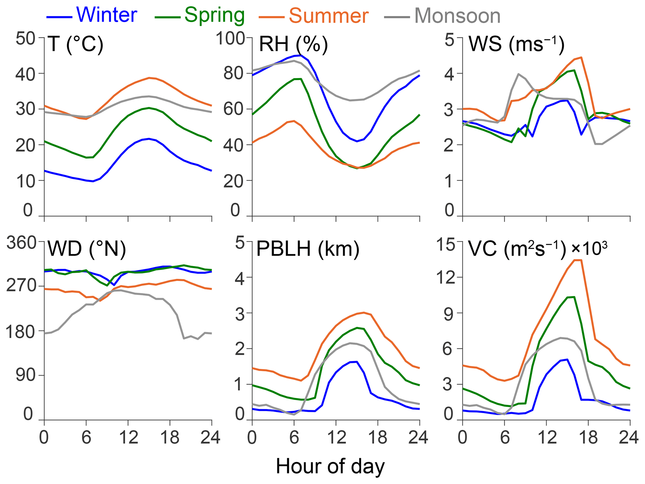
Figure 1Diurnal profiles of meteorological parameters (temperature, relative humidity, wind speed, wind direction, PBLH, and VC) by season. Average values by season and hour of day are presented for all parameters except wind direction. The median value is presented for wind direction. Ventilation coefficient (VC) = PBLH × wind speed.

Download

To investigate the composition of ambient air in New Delhi at high time resolution, we installed a suite of online aerosol measurement instrumentation at the Indian Institute of Technology Delhi (IITD) campus in South Delhi. The instruments are situated in a temperature-controlled laboratory on the top floor of a four-story building. The nearest source of local emissions is an arterial road located 150 m away from the building. We measured chemical composition of nonrefractory PM₁ (NR-PM₁) was measured using an Aerodyne Aerosol Chemical Speciation Monitor (ACSM; Aerodyne Research, Billerica, MA). BC was measured using a multi-channel aethalometer (Magee Scientific Model AE33, Berkeley, CA) with a multi-spot sampling system designed to minimize the filter loading artifact present on earlier aethalometer systems (Drinovec et al., 2015). Particle size distributions (PSDs) were measured using a scanning mobility particle sizer (SMPS; TSI, Shoreview, MN), consisting of an electrostatic classifier (TSI model 3080), a differential mobility analyzer (DMA; TSI model 3081), an X-ray aerosol neutralizer (TSI model 3088), and a water-based condensation particle counter (CPC; TSI model 3785).

2.2 Instrumentation

The instruments were placed on two separate sampling lines. The first sampling line (SL₁) had the ACSM and the SMPS in parallel. The second sampling line (SL₂) was for the aethalometer. Both sampling lines had a PM_2.5 cyclone at the inlet, followed by a water trap and a Nafion membrane diffusion dryer (Magee Scientific sample stream dryer, Berkeley, CA). The flow rate in SL₁ was 3 L min⁻¹, divided as follows: 1 L min⁻¹ pulled by the SMPS, 0.1 L min⁻¹ by the ACSM, and the remaining 1.9 L min⁻¹ by an in-line flow controller which was in parallel with the SMPS and downstream from the ACSM. SL₂ had a flow rate of 2 L min⁻¹ pulled by the aethalometer. For the SMPS, the CPC pulled at a 1 L min⁻¹ flow rate, and the electrostatic classifier was operated at a sheath flow rate of 4 L min⁻¹ to enable SMPS scanning over a broad range of particle sizes. We conducted experiments at multiple sheath flow rates from 4 to 10 L min⁻¹ and found the results to be consistent.

The ACSM measures NR-PM₁, i.e., those compounds that flash vaporize at the heater temperature of ∼600 ^∘C. The flash-vaporized compounds are subsequently ionized in the ACSM via 70 eV electron impact ionization and detected with a quadrupole mass spectrometer (Ng et al., 2011c). The scan speed was set at 200 ms amu⁻¹ and pause setting at 125 for a sampling time (64 s). Detailed operational procedures for the ACSM are provided in Appendix A1. Some submicron aerosol constituents are refractory, including BC, metals, and crustal materials. For our core analyses of PM₁ mass, we use the sum of NR-PM₁ + BC as a composition-based proxy for total PM₁, which we term “C-PM₁”. This C-PM₁ metric excludes the contribution to submicron mass of refractory metals and crustal materials, which we estimate results in a 5 %–10 % underestimate of total PM₁ mass (see below).

2.3 Data processing

The SMPS scanned from 12 to 560 nm, with each subsequent scan 135 s apart. We used a mode fitting algorithm (Hussein et al., 2005) in the mass domain to estimate the PSD between 560 and 1000 nm. We validated the performance of our model by comparing the modeled and observed volume and number concentrations for the observed particle size range. We found that the model predicted the same volume as was observed (slope=1.00, R²=1.00) but slightly overestimated particle number concentrations (slope=1.06, R²=0.96), mostly for smaller particles. In order to develop a supplemental PSD-based estimate of submicron mass, we first estimated a complete (hybrid) PSD up to 1000 nm by combining the observed PSD from 12 to 560 nm and the modeled PSD from 560 to 1000 nm. Estimates of aerosol densities from Asia range between 1.3 and 1.6 g cm⁻³ (Sarangi et al., 2016; Hu et al., 2012). Using a particle density of 1.6 g cm⁻³ and the hybrid PSD, we developed a SMPS-based PM₁ estimate (“SMPS-PM₁”). On an hourly basis, the linear fit between our core C-PM₁ and supplemental SMPS-PM₁ estimates had a slope of 0.96 and an R² of 0.85 (Fig. S1 in the Supplement). This linear fit suggested that our speciated PM₁ data (NR-PM₁ species and BC) agreed reasonably well with the SMPS-PM₁ estimates. We used the PSD to estimate the transmission efficiency (TE) of the ACSM. The details of this correction along with other ACSM data processing steps are provided in Appendix A2. We estimate an overall uncertainty of up to 20 %–25 % in the ACSM data, which is within expectations for measurements from this instrument (Crenn et al., 2015).

While we acquired data for each instrument at high time resolution (∼1 min for the aethalometer and the ACSM; ∼2 min for the SMPS), for analytical simplicity we generally present the hourly averaged data for each instrument in this study. We categorize the seasons as winters (December to mid-February), summers (April to June), the monsoon (July to mid-September), and spring (mid-February to March) (Indian National Science Academy, 2018). Autumn (mid-September to November) is not included in our core analyses due to the unavailability of ACSM data for that period. In our analysis, we define day as 07:00–19:00 and night as 19:00–07:00.

We retrieved the hourly temperature and relative humidity (RH) data from the Indira Gandhi International Airport (IGIA; 8 km from our site). To obtain mesoscale (regional) meteorological data for wind speed, direction (10 m from ground), and planetary boundary layer height (PBLH) in Delhi, we used a NASA meteorological reanalysis dataset, MERRA2 (Gelaro et al., 2017). MERRA2 has a spatial resolution of $\mathrm{0.5}{}^{\circ }\times \mathrm{0.625}{}^{\circ }$ (55 km × 60 km) and an hourly temporal resolution. We retrieved daily precipitation data for Delhi from the European Centre for Medium-Range Weather Forecasts' reanalysis dataset, ERA-Interim (Dee et al., 2011).

The hourly data for all species across the campaign are neither strictly normally nor log-normally distributed (Fig. S2). However, since the data are relatively closer to being log-normally distributed, we have included geometric mean (GM) and geometric standard deviation (GSD) in addition to the arithmetic mean (AM) wherever possible to provide a more complete representation of the central tendency of the data. Furthermore, the annual averages reported in this study are the averages of all the available hourly data from 2017 for the NR-PM₁ species and BC. It should be noted that we do not have ACSM data (NR-PM₁ species) for autumn and only a few days of aethalometer data (BC) for the monsoon. On the basis of available SMPS-PM₁ data (our site) and PM_2.5 data (multiple regulatory monitors in Delhi), we estimate that the true annual average differs from the data we collected by within ±20 %. As a sensitivity analysis, we reconstruct annual and campaign averages by giving equal weight to each 2-month period. For example, to calculate the synthetic (reconstructed) annual average for 2017, we averaged the averages of the six 2-month periods (January–February through November–December). In Table S1 we have provided a comparison between the AM, GM, and the synthetic averages of the PM₁ components for the 2017 data against the entire campaign data.

3.1 Mass concentration

We observed marked seasonal and diurnal variation in the PM mass concentration owing to the interactions of sources, atmospheric mixing, and physicochemical processing. Figure 2 shows the time series of NR-PM₁, individual submicron species, PM_2.5 at a background site, and selected meteorological parameters. The daily average NR-PM₁ concentrations at our site varied between 12.7 and 392 µg m⁻³, with an annual average of 87.3 µg m⁻³. Most C-PM₁ mass was nonrefractory – the average NR-PM₁ fraction of C-PM₁ was highest in the winter (94 %) and lowest for warmer months (85 %) (Fig. 3). The average wintertime NR-PM₁ concentration was ∼2 times higher than spring and ∼4 times higher than the warmer months. Using speciated mass concentrations and the PSD, we observed that C-PM₁ was highly correlated with SMPS-PM₁ (R²=0.83), and we achieved almost complete mass closure (Fig. S1). That most of the PM₁ was composed of nonrefractory material and BC was consistent with past literature from Delhi which observed that metals and other nonrefractory crustal materials, which we did not measure in this study, constituted less than 5 % of PM₁ (Jaiprakash et al., 2017).

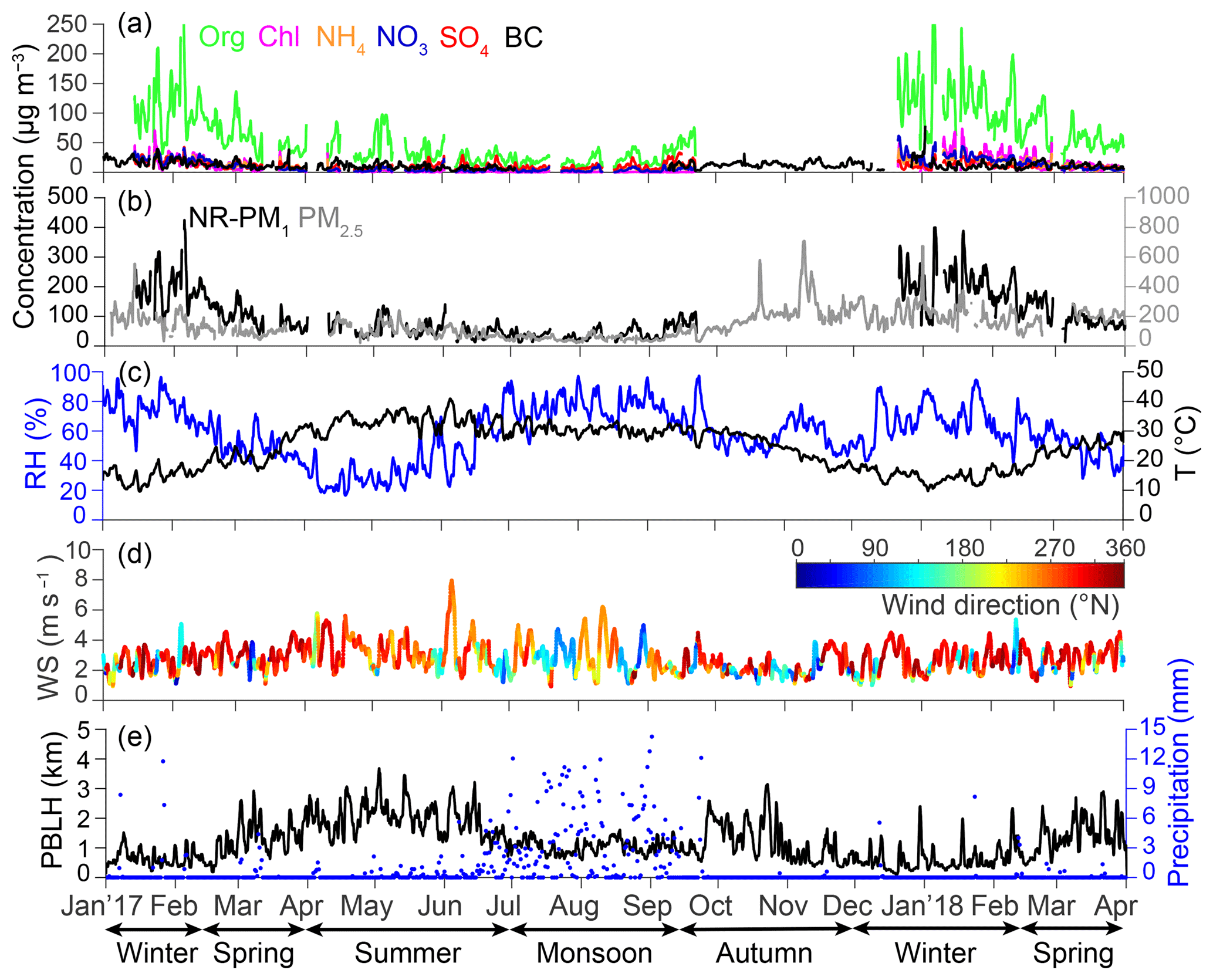
Figure 2Time series of (a) PM₁ species (Org, Chl, NH₄, NO₃, SO₄, and BC), (b) NR-PM₁ and PM_2.5 (DPCC, R.K. Puram – 3 km from our site), (c) relative humidity and temperature, (d) wind speed and direction, and (e) PBLH and precipitation. A 24 h moving average is applied on all time series presented.

Download

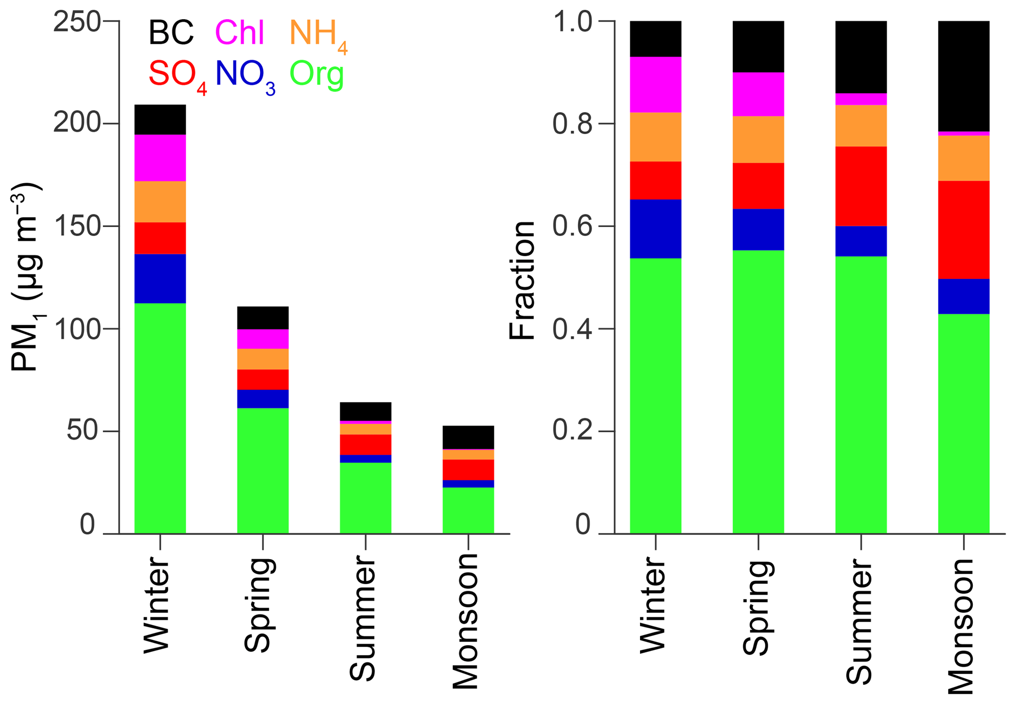
Figure 3Average absolute and fractional composition of PM₁ (Org, Chl, NH₄, NO₃, SO₄, and BC) by season. Limited BC data for the monsoon due to instrument downtime.

Download

We estimated that the C-PM₁ concentrations observed at our site were generally ∼85 % of the PM_2.5 concentrations (R²=0.54 and slope=0.85 for linear fit of hourly C-PM₁ and PM_2.5 concentrations over entire campaign) measured at the nearest monitoring station that is operated by the Delhi Pollution Control Committee (DPCC), R.K. Puram (3 km away), where the annual average PM_2.5 concentration for 2017 was 140 µg m⁻³. There were strong seasonal and diurnal variations in mass loadings, with winter being the most polluted with average concentration ∼4 times higher than the least polluted summer and monsoon months. The daily average PM_2.5 concentration exceeded the daily average Indian National Ambient Air Quality Standards (NAAQS; 60 µg m⁻³) on more than 80 % of the days and the World Health Organization (WHO) 24 h average air quality guidelines (25 µg m⁻³) on all but two days. A distinct feature of Delhi's wintertime air pollution is the nearly complete absence of periods of clean air, in contrast to some other polluted megacities (e.g., Beijing), which are characterized by episodic alternation between clean and polluted conditions (Sun et al., 2013). For wintertime, the daily average PM_2.5 concentrations exceeded 100 µg m⁻³ on 94 % of the days, the Indian NAAQS on 99 % of the days, and the WHO guidelines on all days. Daily-average PM_2.5 concentrations at R.K. Puram exceeded 500 µg m⁻³ on four days in 2017.

3.2 PM₁ composition: seasonal and diurnal variation

The concentrations and fractional contribution to PM₁ of each species varied by season and time of day. Over the campaign, organics comprised 54 % of the submicron mass, inorganics (chloride, ammonium, nitrate, and sulfate) 36 %, and BC 10 %. There was a strong seasonality in C-PM₁ loadings, with the wintertime average loadings exceeding the relatively less polluted and warmer summer and monsoon months by 3–4 times. We report the average seasonal concentrations of organics, sulfate, ammonium, nitrate, chloride, and BC in Table 1 and their contribution to C-PM₁ in Fig. 3. Within each season there were distinct diurnal (time-of-day) trends for the average concentrations by hour of day for NR-PM₁ and PM₁ components (Fig. 4). These diurnal swings of the average hourly concentrations were the most prominent for the colder winter and spring months. In winter, average hourly NR-PM₁ concentrations ranged between 97.4 and 254 µg m⁻³ (minimum and maximum concentrations for the average diurnal cycle). Spring conditions were moderately less polluted, with hourly average concentrations ranging diurnally from 37.0 to 167 µg m⁻³. The NR-PM₁ concentrations varied much less during summer (range of concentrations for an average diurnal cycle: 38.7 to 72.4 µg m⁻³) and the monsoon (32.1 to 47.7 µg m⁻³). For most seasons, the hourly averaged NR-PM₁ concentrations peaked around 07:00–08:00 and then again around 21:00–22:00, with the daily minimum typically occurring around 15:00–16:00. However, for the monsoon months the NR-PM₁ average hourly concentrations were similar throughout the day. The diurnal variation in average hourly concentrations and fractional composition of NR-PM₁ species for each season is presented in Fig. 5. The day and night averages by season for each PM₁ species along with the summary averages of meteorological parameters are presented in Table 2. We did not observe any marked day of the week difference in the levels or composition of C-PM₁ (Fig. S3).

Table 1Seasonal summary of PM₁ species – arithmetic mean (AM), geometric mean (GM), and geometric standard deviation (GSD) for hourly concentrations.

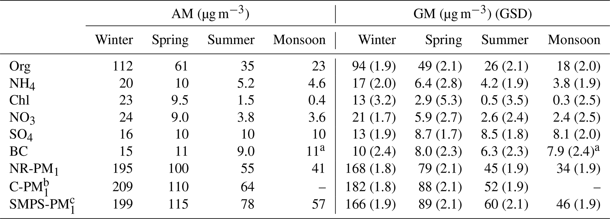
^a Based on limited BC data for the monsoon due to instrument downtime. ^b Composition-based estimate of PM₁ (BC + NR-PM₁). ^c SMPS-based estimate using hybrid PSD and assuming a density of 1.6 g cm⁻³.

Download Print Version | Download XLSX

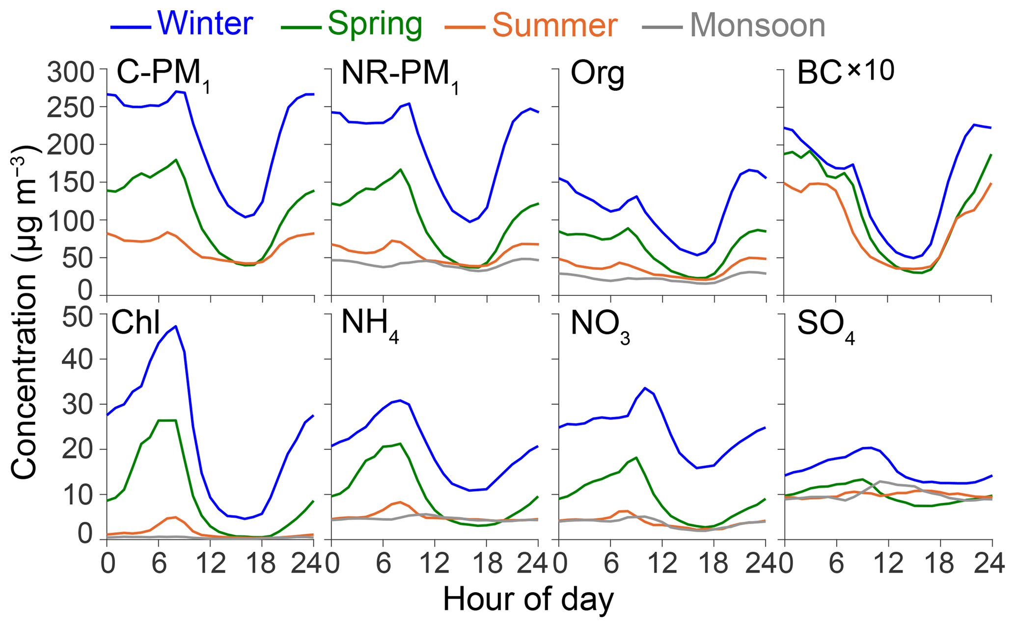
Figure 4Average diurnal profiles of PM₁ species by season. Limited BC data for the monsoon due to instrument downtime. Composition-based estimate of PM₁ (C-PM₁) = BC + NR-PM₁.

Download

Figure 5Stacked average absolute and fractional diurnal profiles of NR-PM₁ species by season.

Download

Table 2Day and night summary of PM₁ species and meteorological parameters. Arithmetic mean used for all species and parameters, except wind direction for which we used median to estimate its central tendency.

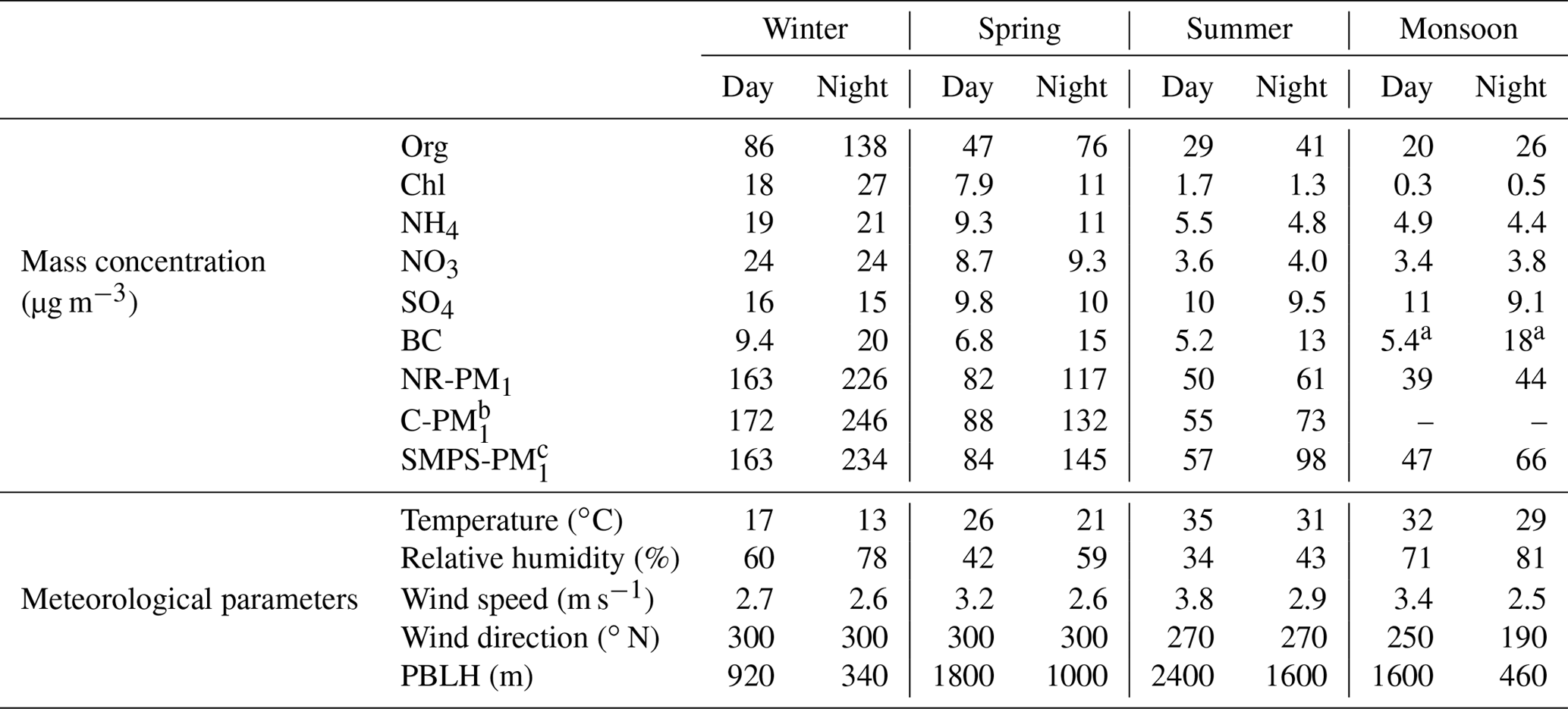
^a Based on limited BC data for the monsoon due to instrument downtime. ^b Composition-based estimate of PM₁ (BC + NR-PM₁). ^c SMPS-based estimate using hybrid PSD and assuming a density of 1.6 g cm⁻³.

Download Print Version | Download XLSX

Organics were the single largest C-PM₁ mass component for all seasons and at all times of the average diurnal cycle. Organics consistently contributed to more than ∼50 % of seasonal C-PM₁ mass, with some episodes when their contribution was as high as 80 %. The high organic fraction of PM is consistent with studies from across the world (Zhang et al., 2007; Jimenez et al., 2009). The daily averages of organics at our site varied between 6.4 and 293 µg m⁻³, with an annual average of 51.5 µg m⁻³. The average wintertime organic concentration was ∼2 times higher than spring and ∼4–5 times higher than summer and the monsoon. While the wintertime organic concentrations ranged between 53.3 and 166 µg m⁻³, with the highest concentration during the night, the diurnal variations were less dynamic for the warmer months, with the hourly average organic concentrations ranging between 20.8 and 49.8 µg m⁻³ for summertime. Comparing daytime and nighttime f₄₃ and f₄₄ values for each season, the bulk organic aerosol was generally more oxidized during the warmer periods (Fig. S4), presumably owing to the higher photochemical activity during that time (Ng et al., 2011a).

Ammonium was the prominent inorganic cation in C-PM₁ and generally balanced all the anionic inorganic species (chloride, nitrate, and sulfate). Over the campaign, the molar ratio of the inorganic anions to cations (ammonium) was 0.82 (R²=0.96). Ammonium mass concentrations were consistently around ∼10 % of the observed C-PM₁. The daily average of ammonium at our site varied between 1.5 and 37.9 µg m⁻³, with an annual average of 9.0 µg m⁻³. The average ammonium concentration for wintertime was ∼2 times higher than spring and ∼4 times higher than summer and the monsoon. Ammonium concentration hourly averages ranged between 10.9 and 30.8 µg m⁻³ during the winter and between 4.2 and 8.3 µg m⁻³ during the summer.

We observed some of the highest chloride concentrations reported anywhere in the world, with episodes when hourly averages exceeded 100 µg m⁻³ (more than 40 such hours across the campaign). The 90th and 95th percentile values of the hourly concentrations of chloride over the campaign were 26.7 and 43.8 µg m⁻³, respectively. The daily average of chloride concentration at our site varied between 0.1 and 66.6 µg m⁻³, with an annual average of 6.1 µg m⁻³. Chloride concentrations showed the strongest seasonal variability, with the average wintertime concentration ∼2 times higher than during spring and more than 20 times higher than during the warm (summer and monsoon) months. During the cooler winter and spring months, chloride concentrations had the largest diurnal variation among all PM species observed, with the average diurnal minimum and maximum hourly concentration ranging between 4.6 and 47.3 µg m⁻³ in wintertime. The winter chloride peak is notable for its timing in the early morning hours (∼ 07:00), which is considerably later than the diurnal peak in organics and BC, which tended to occur shortly before midnight. While chloride contributed more than 10 % of the submicron mass in the winters, it comprised less than 2 % of the C-PM₁ mass concentration during the summer and monsoon. Furthermore, chloride constituted around 12 %–16 % of NR-PM₁ for temperatures below 15 ^∘C but dropped to less than 4 % of the NR-PM₁ concentrations for temperatures above 25 ^∘C (Fig. S5). Given that ammonium was nearly always present in sufficient quantities to neutralize the major inorganic anions measured by the ACSM, we infer that the dominant fraction of chloride was usually present as ammonium chloride, for which gas–particle partitioning is strongly temperature dependent. (However, we cannot exclude the possibility that organic chlorides contributed a subsidiary fraction of the chloride mass.) Even for high episodic chloride concentrations, ammonium was present in sufficient levels to neutralize most of the anionic species, with a deficiency of only ∼20 % when considering only hours with chloride concentrations higher than the 90th percentile campaign value (26.7 µg m⁻³).

To understand whether the sharp drop in chloride concentrations for warmer times of day could be explained by evaporation of ammonium chloride, we used an inorganic aerosol thermodynamics model (Friese and Ebel, 2010). The detailed methodology and results of the model used are presented in Appendix B. Results from inorganic thermodynamic modeling suggest that most of the ammonium chloride observed in the winter is expected to evaporate at summer temperatures and relative humidity, consistent with our observations. The volatile nature of ammonium chloride has also been observed in other parts of the world (Salcedo et al., 2006; Wang et al., 2016) and was consistent with the sharp drop in the chloride fraction that we observed for the warmer periods. We believe that gas–particle partitioning and episodic sources (Sect. 3.4.1) may drive much of the diurnal and seasonal variation in particulate chloride. We would therefore expect a large fraction of chloride to be in the gas phase, especially for warmer periods. We did not collect gas-phase HCl measurements here, but future studies could validate this hypothesis through measurements of gas-phase chloride.

Nitrate comprised 6 %–12 % of Delhi's C-PM₁, with daily averages between 0.6 and 58.5 µg m⁻³, with an annual average of 8.8 µg m⁻³. The average wintertime nitrate concentration was more than 2 times higher than spring and more than 6 times higher than summer and the monsoon. The average diurnal cycle (lowest and highest hourly average concentration) for wintertime concentrations ranged between 15.9 and 33.6 µg m⁻³, and the summer concentrations ranged between 2.2 and 6.3 µg m⁻³. The nitrate fraction of NR-PM₁ dropped from 12 % at temperatures below 25 ^∘C to 5 %–9 % at temperatures above 25 ^∘C, likely due to the thermodynamics of ammonium nitrate. As with chloride, nitrate concentrations were also generally highly correlated with ammonium concentrations (R²=0.69 for hourly data over entire campaign), suggesting that most of the nitrate observed was present as ammonium nitrate. Considering the ubiquitous NO_x sources in this megacity, organic nitrates may also contribute to the total nitrate measured by the ACSM.

The daily averages of sulfate at our sites varied between 3.1 and 34.5 µg m⁻³, with an annual average of 11.8 µg m⁻³. Sulfate had the least seasonal variability among the NR-PM₁ species, with wintertime average concentration ∼1.5 times higher than each of the other seasons (spring, summer, and monsoon). In addition to the low seasonal variability, sulfate was also the chemical constituent with the least diurnal variation and had relatively higher daytime concentrations for the warmer summer months. The diurnal variation in sulfate concentration for the cooler months was similar to that of other PM₁ species, with the average early morning concentrations for winter and spring almost 2 times higher than the daytime concentrations. Sulfate was the only NR-PM₁ species that had a higher mass fraction during the warmer months, contributing 13 %–30 % to the C-PM₁ mass in the warmer months, 8 %–20 % in spring, and 5 %–13 % in winter, with the mass fraction being highest during the daytime for all seasons. The sulfate fraction of NR-PM₁ increased from less than 10 % for periods cooler than 25 ^∘C to more than 25 % for periods above 35 ^∘C. The increase in sulfate mass fraction for warmer periods can be explained by the lower diurnal and seasonal variability in its absolute concentration, possibly due to a combination of increased daytime photochemical formation rates for warmer months and sulfate being well mixed in the atmosphere because of its transport from longer distances (Verma et al., 2012).

BC contributed to 6.4 % of the C-PM₁ mass concentration in the winter compared to 10 % in the spring and 14 % in the summer. We had limited monsoon data for BC. The daily average of BC at our site varied between 2.2 and 35.2 µg m⁻³, with an annual average of 12.4 µg m⁻³. The average wintertime BC concentration was ∼1.5 times higher than spring and summer. The seasonal differences in the absolute BC concentrations were not as high as any of the other PM₁ species. One possible explanation for this result relates to the presence of nearby BC sources within Delhi, including the major ring road with truck traffic near our sampling site. These trucks are often restricted to only passing through Delhi at night (Guttikunda and Calori, 2013). It is plausible that these nearby primary emissions would be incompletely mixed into the boundary layer and are therefore relatively less affected by atmospheric mixing (Sect. 3.3 and 3.5). Accordingly, BC had sharp diurnal variability, with peak nocturnal BC concentrations typically ∼3–4 times higher than during midday hours, with peak concentrations occurring at a similar time to the temporal peak for organics (typically just before midnight).

3.3 Role of meteorology

The planetary boundary layer height (PBLH) had a strong seasonal variation with summer heights 2–4 times larger than those during the cooler months. The seasonal variability in the PBLH along with that in wind speed resulted in the ventilation coefficient (VC = PBLH × wind speed, sometimes referred to as normalized dilution rate) being 4–6 times slower for the wintertime compared to the summer. The VC is often used as a parameter to characterize the role of atmospheric dilution in pollutant concentrations, both in the Indian context (Vittal Murty et al., 1980) and globally (Marshall et al., 2005; Apte et al., 2012). Seasonal variability in the VC appears to reasonably agree with the higher NR-PM₁ concentrations in less ventilated cold months and lower concentrations in the warmer months when the VC was higher (Fig. 6). The week with the lowest VC was ∼6 times less ventilated than the most ventilated week and had ∼6 times higher NR-PM₁ mass concentrations. For the non-monsoon periods, the VC was generally a good indicator of NR-PM₁ concentrations (R²=0.56 for weekly averaged data). For the cooler winter and spring months, the R² for the linear fit of the weekly averaged VC and NR-PM₁ concentrations was 0.79. The monsoon concentrations were lower than those that would be expected by the VC calculated for those periods. This result could be explained by a combination of change in the prominent nighttime wind direction from northwest to south during the monsoon and the washout of PM by the monsoon rain. For the monsoon period, we observed that the average NR-PM₁ mass concentration was almost half on days when it rained compared to the dry (no rain) days with no change in the composition of NR-PM₁. The strong modulating effect of meteorology on air pollution is well appreciated for Delhi and other Indian cities (Guttikunda and Gurjar, 2012; Tiwari et al., 2015; Sujatha et al., 2016).

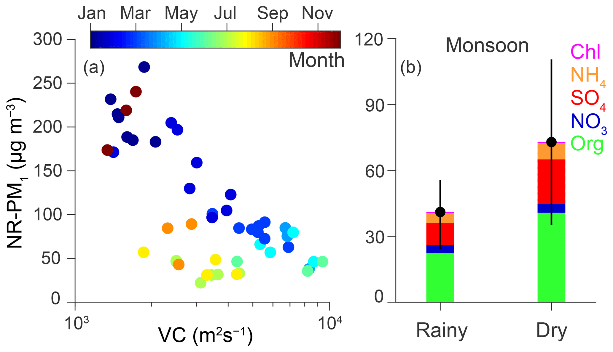
Figure 6(a) Variations of NR-PM₁ mass concentrations as a function of ventilation coefficient. Each scatter point is a weekly average and is color coded by month. Note that July to mid-September is the monsoon season. (b) Average NR-PM₁ composition for days with (rainy) and without rain (dry). The vertical lines are the 25th (bottom) and 75th (top) percentiles.

Download

Even within each season, the VC showed large time-of-day variations, with highest hourly average values 5–10 times larger than the lowest. For each season, times of day with a lower VC had the highest NR-PM₁ concentrations, and the concentrations decreased as the VC value increased (Fig. S7). The large diurnal range of the VC seemed to explain most of the variability in NR-PM₁ concentrations by time of day for most seasons ($R_{\mathrm{winter}}^{\mathrm{2}}=\mathrm{0.88}$; $R_{\mathrm{spring}}^{\mathrm{2}}=\mathrm{0.93}$; $R_{\mathrm{summer}}^{\mathrm{2}}=\mathrm{0.81}$). For the monsoon, the diurnal variability of most PM₁ species was generally low, even though the VC varied by time of day, possibly due to precipitation washout of PM and a change in characteristic wind direction during the monsoon (as discussed above).

In general, the sharp variation in the VC by season and time of day appear to explain much of the variability in NR-PM₁ concentrations. Furthermore, volatile species (e.g., ammonium chloride and ammonium nitrate) evaporate to the gas phase during warmer periods, further lowering the mass concentrations compared to the cooler periods. While there are seasonal differences in emissions from sources such as crop burning and local biomass burning for heat (Guttikunda and Calori, 2013), our analysis suggests that in addition to episodic sources, meteorology being unfavorable is an important factor for some of the high PM concentrations observed.

3.4 Episodic high concentrations

3.4.1 Chloride episodes and wind direction

Delhi experiences a prominently northwestern wind (Fig. 1). However, we observed that for brief periods during winter and spring when the wind was from the south, the peak chloride concentrations dropped from as high as 50–100 µg m⁻³ on one day to less than 10 µg m⁻³ on the next (Fig. 7). Furthermore, the highest decile of chloride concentrations in the campaign were mostly observed when the wind was from the northwest (Fig. 8). During winter mornings, when chloride concentrations were generally highest, the chloride fraction of C-PM₁ was almost 2 times higher for periods with a northwestern wind compared to periods with wind from any other direction (Fig. S8). These findings suggest a large source of chloride in the northwest of Delhi. The high levels of chloride observed in Delhi are neither observed in other South Asian countries (Kim et al., 2015; Stone et al., 2010; Salam et al., 2003), nor in other parts of India (Gupta and Mandariya, 2013; Guttikunda et al., 2013; Gupta et al., 2007), suggesting that these extreme levels of chloride probably come from more than just the usual type of biomass and waste burning (Goetz et al., 2018), which is ubiquitous across South Asia (Streets et al., 2003). While filter-based studies can cause underreporting of volatile species such as ammonium chloride, the levels of chloride we observe in Delhi are much higher than those reported from studies in South Asia (outside Delhi) that use online aerosol instrumentation (Goetz et al., 2018; Chakraborty et al., 2015). Furthermore, the PMF factor for biomass burning organic aerosol of Bhandari et al. (2019) does not correlate with chloride. There are many industrial sites in the northwest of Delhi, including metal processing plants that use HCl for steel pickling (Jaiprakash et al., 2017). The fugitive HCl fumes from these industries along with the high ammonia in Delhi (Warner et al., 2017) could be a pathway for these high observed particulate chloride concentrations (Pio and Harrison, 1987). Other possible sources of HCl are from the combustion of polyvinyl chloride, coal, and biomass burning (Yudovich and Ketris, 2006; Lightowlers and Cape, 1988; Palmer, 1976). Our findings are based on measurement of particulate chloride and inorganic thermodynamic modeling and can be tested by future studies that measure both gas and particulate chloride.

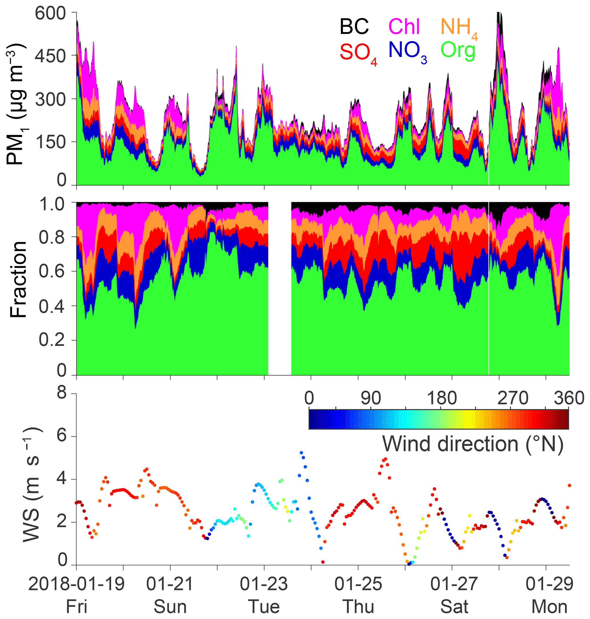
Figure 7Time series of PM₁ species (Org, Chl, NH₄, NO₃, SO₄, and BC) – stacked absolute concentrations and fraction of PM₁ – along with wind speed and wind direction for a period with high chloride concentrations.

Download

Figure 8Relative frequency for high episodic concentrations of PM₁ species (concentrations greater than the 90th percentile concentration of that species for the entire campaign) as a function of the wind direction.

Download

3.4.2 High organic episode

While organics contributed to almost half of the C-PM₁ for all seasons and times of day, there were episodes for which the contribution of organics increased to as high as 80 % of the C-PM₁. One such episode was around Lohri (13 January 2018), a festival celebrated in many parts of north India (including Delhi and regions upwind of Delhi), with bonfires burnt at night. In 2018, Lohri was on a weekend (Saturday), and we observed a sharp increase in nighttime C-PM₁ concentrations, almost 2–3 times higher than the weekday nights preceding Lohri (Fig. 9). The contribution of both organics and BC increased for this period, with organics concentrations as high as 300 µg m⁻³ during these bonfire nights, contributing to ∼60 %–70 % of the C-PM₁.

Figure 9Time series of PM₁ species (Org, Chl, NH₄, NO₃, SO₄, and BC) – stacked absolute concentrations and fraction of PM₁ – for a period with high organic PM concentration coinciding with the Lohri bonfire festival of 15 January 2018.

Download

3.5 Primary vs. secondary organic aerosol

Positive matrix factorization (PMF) conducted on the ACSM mass spectra provided further information on the sources and atmospheric processes that affect NR-PM₁ concentrations in Delhi (Bhandari et al., 2019). The organic aerosol (OA) was separated into two factors: primary OA (POA) and oxygenated OA (OOA), with periods when the POA factor further separated into hydrocarbon-like OA (HOA) and biomass-burning OA (BBOA). POA exhibited strong diurnal variability, reflecting the impact of primary combustion emissions modulated by diurnal cycles in the PBLH. The POA fraction of organics was generally highest during the nighttime (∼50 % for winter and ∼40 % for summer) and lowest during the daytime (∼20 % for both winter and summer). As observed in other megacities, OOA was the largest constituent of the organic aerosol throughout the year (Jimenez et al., 2009), demonstrating the profound influence of secondary formation on particle concentrations in Delhi. OOA contributed to 50 %–80 % of the organics almost year-round (Fig. S9). We estimated primary particulate matter ($\mathrm{PPM}=\mathrm{POA}+\mathrm{Chl}+\mathrm{BC}$) and secondary particulate matter ($\mathrm{SPM}=\mathrm{OOA}+{\mathrm{NH}}_{\mathrm{4}}+{\mathrm{NO}}_{\mathrm{3}}+{\mathrm{SO}}_{\mathrm{4}}$) following Sun et al. (2013). Since chloride was considered primary, and ammonium was generally highly correlated with chloride, we apportioned a chloride-equimolar amount of ammonium as primary and the remaining as secondary organic aerosol. In Fig. 11 we separate C-PM₁ into PPM and SPM by season and time of day. We observed that almost 50 %–70 % of Delhi's C-PM₁ was secondary in nature for the winter and spring months and up to 60 %–80 % for the warmer summer and monsoon months. Our results show that secondary aerosol accounts for the dominant fraction of Delhi's ambient NR-PM1 under most conditions. While our analyses do not provide direct evidence for the origin of the secondary fraction of PM₁, consideration of typical advection timescales from the upwind boundaries of Delhi (∼2–3 h at typical wind speeds) suggests that a substantial fraction of Delhi's secondary aerosol may be transported from upwind regions, which also experience high PM mass loadings (Guttikunda and Goel, 2013). These findings suggest that improving Delhi's air quality will require a concerted effort at both at the local and the regional level. Future work could usefully apportion the composition of PM₁ at receptor sites upwind of Delhi.

BC was found to be well correlated (R²=0.65) with HOA (for periods when HOA was a separate factor) (Bhandari et al., 2019), suggesting that traffic, diesel generators, and other liquid fossil fuel combustion contribute substantially to the BC inventory for Delhi. Furthermore, unlike chloride, the highest BC concentrations were uncorrelated with any particular wind direction (Fig. 8) and also showed less seasonal variation than other PM₁ species (Fig. 4), potentially indicating a nearby year-round source that was less affected by atmospheric mixing. We suspect that trucks (and other diesel vehicles) were a major source of the high BC concentrations that we observed, similar to what has been observed in other urban environments in India (Latha et al., 2004). While BC absolute concentrations did not vary as much as other PM₁ species, the fractional contribution to BC was as high as 20 % during periods when the C-PM₁ was lower (Fig. 10). These findings indicate the large local nature of BC emissions and the potential to reduce BC concentrations by targeting high emitters such as heavy-duty trucks and diesel generation systems (Baidya and Borken-Kleefeld, 2009). Previous studies have shown that a small fraction (10 %–20 %) of high-emitting heavy-duty trucks contribute to almost half of the total BC emissions from heavy-duty trucks (Ban-Weiss et al., 2009).

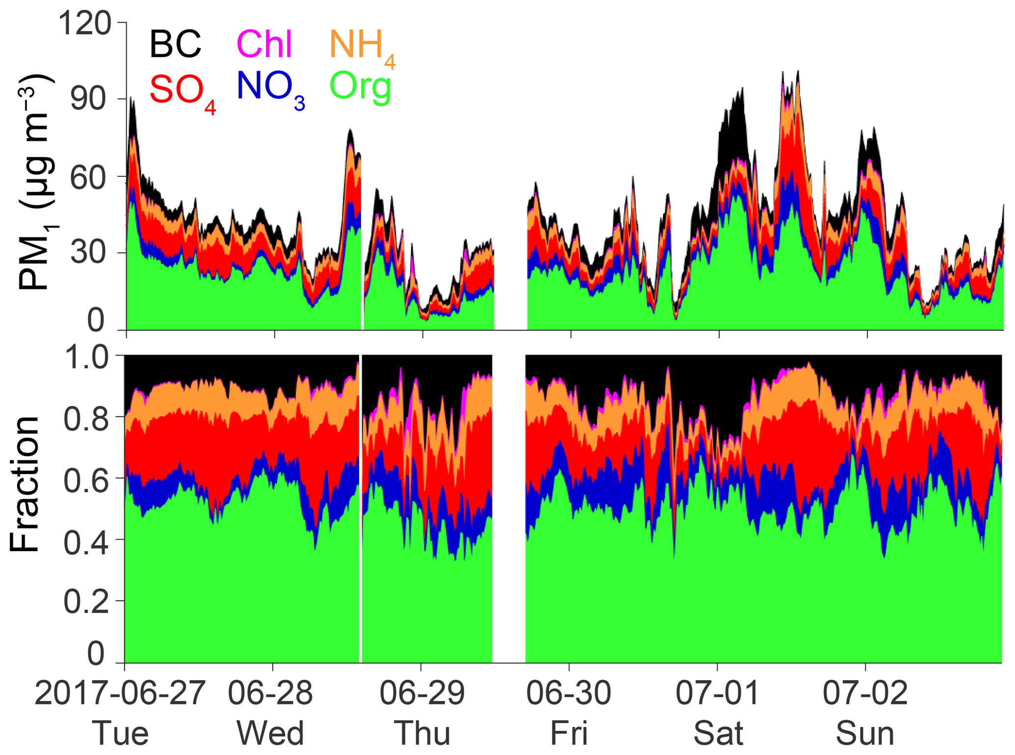
Figure 10Time series of PM₁ species (Org, Chl, NH₄, NO₃, SO₄, and BC) – stacked absolute concentrations and fraction of PM₁ – for a relatively less polluted (warm) period.

Download

Figure 11Average diurnal variation of mass concentrations and mass fractions of primary and secondary C-PM₁ by season.

Download