the Creative Commons Attribution 4.0 License.
the Creative Commons Attribution 4.0 License.
 | 21 May 2019
Antarctic clouds, supercooled liquid water and mixed phase, investigated with DARDAR: geographical and seasonal variations
Constantino Listowski
Julien Delanoë
Amélie Kirchgaessner
Tom Lachlan-Cope
John King
Antarctic tropospheric clouds are investigated using the DARDAR (raDAR/liDAR)-MASK products between 60 and 82∘ S. The cloud fraction (occurrence frequency) is divided into the supercooled liquid-water-containing cloud (SLC) fraction and its complementary part called the all-ice cloud fraction. A further distinction is made between SLC involving ice (mixed-phase clouds, MPC) or not (USLC, for unglaciated SLC). The low-level (<3 km above surface level) SLC fraction is larger over seas (20 %–60 %), where it varies according to sea ice fraction, than over continental regions (0 %–35 %). The total SLC fraction is much larger over West Antarctica (10 %–40 %) than it is over the Antarctic Plateau (0 %–10 %). In East Antarctica the total SLC fraction – in summer for instance – decreases sharply polewards with increasing surface height (decreasing temperatures) from 40 % at the coast to <5% at 82∘ S on the plateau. The geographical distribution of the continental total all-ice fraction is shaped by the interaction of the main low-pressure systems surrounding the continent and the orography, with little association with the sea ice fraction. Opportunistic comparisons with published ground-based supercooled liquid-water observations at the South Pole in 2009 are made with our SLC fractions at 82∘ S in terms of seasonal variability, showing good agreement. We demonstrate that the largest impact of sea ice on the low-level SLC fraction (and mostly through the MPC) occurs in autumn and winter (22 % and 18 % absolute decrease in the fraction between open water and sea ice-covered regions, respectively), while it is almost null in summer and intermediate in spring (11 %). Monthly variability of the MPC fraction over seas shows a maximum at the end of summer and a minimum in winter. Conversely, the USLC fraction has a maximum at the beginning of summer. However, monthly evolutions of MPC and USLC fractions do not differ on the continent. This suggests a seasonality in the glaciation process in marine liquid-bearing clouds. From the literature, we identify the pattern of the monthly evolution of the MPC fraction as being similar to that of the aerosols in coastal regions, which is related to marine biological activity. Marine bioaerosols are known to be efficient ice-nucleating particles (INPs). The emission of these INPs into the atmosphere from open waters would add to the temperature and sea ice fraction seasonalities as factors explaining the MPC fraction monthly evolution.


Antarctic clouds need to be correctly represented in regional and global atmospheric models to improve daily operational forecast as well as future global climate predictions. Clouds' contribution to Antarctica's ice mass balance via precipitation and to the Antarctic surface energy budget are poorly constrained. However, it has been shown that they exert a warming effect on the ice sheet (Scott et al., 2017; Nicolas et al., 2017). The microphysical properties of clouds can also affect circulation at much lower latitudes due to the changes they induce in the energy budget and the meridional temperature gradients (Lubin et al., 1998). In the Southern Ocean (SO) and Antarctic seas, clouds cause major radiative biases in climate prediction models (Haynes et al., 2011; Flato et al., 2013; Bodas-Salcedo et al., 2014; Hyder et al., 2018). The supercooled liquid water causes major difficulties in cloud microphysics modelling over the SO (Bodas-Salcedo et al., 2016). It is difficult to conceive that the SO energy budget's long-standing dilemma can be solved without paying close attention to clouds in the Antarctic region (60–90∘ S), which is the southern boundary of the SO and more generally the cold sink of our planet. In Antarctica, surface radiation biases of several tens of watt per square metre are derived from mesoscale high-resolution models, which point to major problems in the simulation of the cloud cover (Bromwich et al., 2013a) and of the cloud thermodynamic phase and more particularly of the supercooled liquid water (the water staying in the liquid phase below the freezing point) (Lawson and Gettelman, 2014; King et al., 2015; Listowski and Lachlan-Cope, 2017). Ultimately, the right balance of ice vs. liquid mass in Antarctic clouds in high-resolution models will largely depend on the way the ice microphysics is implemented, the way it leaves or removes the formed supercooled liquid water (Listowski and Lachlan-Cope, 2017), and how processes like secondary ice multiplication observed in that region (Grosvenor et al., 2012; Lachlan-Cope et al., 2016; O'Shea et al., 2017) can be correctly accounted for (Young et al., 2019). This balance will in turn determine the ability of the model to minimise the surface radiative biases. Improving the modelling of the supercooled liquid water over the region may induce drastic changes in the simulations of clouds in the SO (Lawson and Gettelman, 2014), without being certain that any improvement for one part of the region will also lead to the improvement of cloud modelling over the rest of the Antarctic. Hence, being able to track the Antarctic-wide formation of supercooled liquid and the mixed phase and adding to the efforts of ground-based observation studies (Lawson and Gettelman, 2014; Scott and Lubin, 2014; VanTricht et al., 2014; Gorodetskaya et al., 2015; Silber et al., 2018) appear to be necessary steps towards improve cloud microphysics modelling in the Antarctic for lowering the surface radiative biases across the regions that are observed in the climate prediction models (e.g. Lenaerts et al., 2017).
Because of the remoteness of the continent, the harsh environment to which every ground or aircraft operation is exposed, and the inaccessibility of most of Antarctica to in situ observations, satellite observations appear as a welcome if not crucial complement. For instance, Palerme et al. (2014) used satellite radar products to build the first climatology of snowfall rates across the Antarctic continent (updated by Palerme et al., 2019). Nonetheless, a few airborne and ground-based campaigns took place in the last 10 years, presenting new cloud and precipitation studies that unveiled cloud or precipitation properties in different regions like the Antarctic Peninsula (Grosvenor et al., 2012; Lachlan-Cope et al., 2016), the Weddell Sea (O'Shea et al., 2017), the West Antarctic Ice Sheet (Scott and Lubin, 2014; Silber et al., 2018), Adélie Land (Grazioli et al., 2017a, b; Genthon et al., 2018), Dronning Maud Land (Gorodetskaya et al., 2015) or the South Pole (Lawson and Gettelman, 2014). In order to get the needed wider perspective on the Antarctic-wide geographical distribution and seasonal variation in the cloud thermodynamic phase and the supercooled liquid water, we make use of the synergetic DARDAR (raDAR/liDAR) products (Delanoë and Hogan, 2010; Ceccaldi et al., 2013), which were recently used for mapping the Arctic mixed-phase clouds (Mioche et al., 2015). Bromwich et al. (2012), who gave a review on all aspects of tropospheric Antarctic clouds, illustrated the strength of using active remote sensing over passive remote-sensing systems to correctly capture cloud cover over icy terrain and especially over the Antarctic continent. Previous studies used other radar–lidar satellite products to describe the horizontal and vertical distribution of clouds in the SO and the Antarctic during the 2007–2009 period (Verlinden et al., 2011), the ice microphysical properties and the cloud distribution in the Antarctic during the 2007–2010 period (Adhikari et al., 2012). Jolly et al. (2018) described the cloud and phase distribution over the Ross Sea and the Ross Ice Shelf (RIS) according to a classification of dynamical regimes evidenced in previous works. However, it is the first time that the DARDAR products are used in that region. More particularly, we aim to describe the Antarctic-wide cloud geographical and seasonal variation on a monthly to seasonal scale with a specific focus on the supercooled liquid water (SLW).
In Sect. 2 we recall the main features of the Antarctic atmosphere, and in Sect. 3 we present the data and the method we use. In Sect. 4 we present results on the seasonal, geographical and vertical variations of different cloud types, as well as the monthly variations over specific regions. We also present comparisons made with ground-based measurements taken over our period of interest. Finally, we investigate links with the sea ice fraction for the different cloud phases. In Sect. 5, we discuss the results and, importantly, the link between the seasonality of mixed-phase clouds and the sea ice fraction and provide an explanation of the observed monthly time series for these clouds. Section 6 concludes and recalls our main results.
We recall the salient features of the Antarctic environment, focusing on our 4 years of interest (2007–2010; see Sect. 3). Antarctica is characterised by a very contrasted topography illustrated in Fig. 1. Recall that “Antarctica” refers to the continent while “Antarctic” refers to the whole region, including the ocean (60–82∘ S in this study). West Antarctica (WA) has the lowest average surface height, with a peak altitude at around 2.5 km above sea level (a.s.l.) in the interior of the West Antarctic Ice Sheet (WAIS). East Antarctica (EA) hosts the Antarctic Plateau, which reaches altitudes of 4 km a.s.l.

Figure 1The Antarctic continent (Antarctica) and its topography (Fretwell et al., 2013), along with names of places mentioned in this study. The Transantarctic (TA) Mountains separate West Antarctica (WA) from East Antarctica (EA). Two ice shelves are also reported: the Ross Ice Shelf (RIS) and the Amery Ice Shelf (AIS). MBL stands for Marie Byrd Land and PEL for Princess Elisabeth Land. Bellings. refers to Bellingshausen. The location of two UK, one French–Italian and one US Antarctic stations are indicated with markers: Rothera (triangle), Halley VI (circle), Concordia (square) and Amundsen–Scott South Pole Station (diamond shape). Measurements made at these stations are used in Sect. 4.4.
Antarctica is surrounded by an uninterrupted stream of westerlies favoured by the lack of land as illustrated by the isobars of the mean sea level pressure (MSLP) depicted in Fig. 2a. We used ERA-Interim reanalysis monthly average products (Dee et al., 2011) averaged over 2007–2010 for each season. There are three permanent (climatic) low-pressure systems (King and Turner, 1997), with average positions that are essentially determined by the topography of the continent (Baines and Fraedrich, 1989). The most obvious of these lows is the Amundsen Sea low (ASL) to the west of the continent, across the Amundsen and the Ross seas around 140∘ W (Fig. 2a–d). The two other lows are located around 100∘ E (see in Fig. 2b and c) and around 30∘ E (see in Fig. 2a and c).
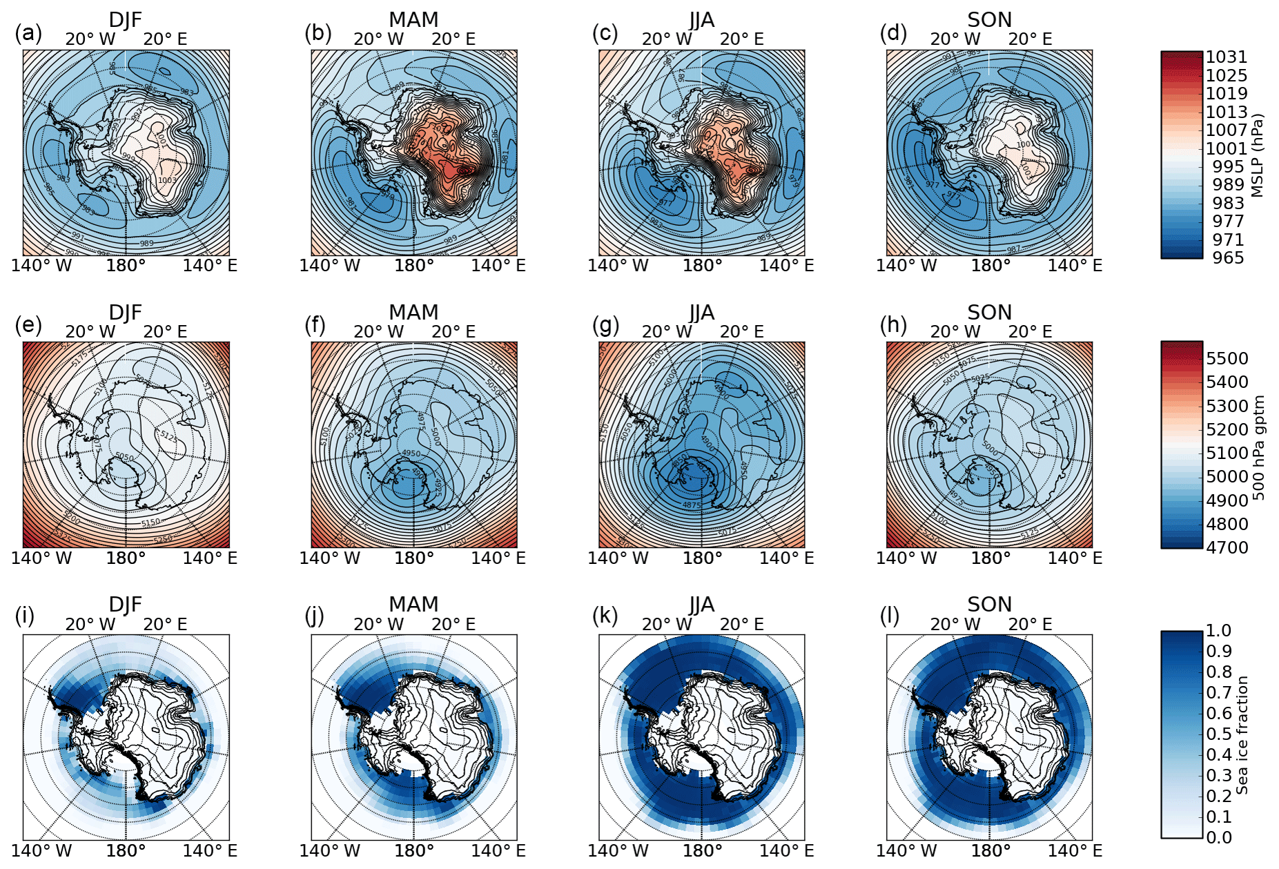
Figure 2Four-year (2007–2010) seasonal averages of (a–d) the mean sea level pressure (MSLP, in hPa), (e–h) the 500 hPa geopotential height (m). Panels (i–l) show the 4-year seasonal average of the sea ice fraction obtained from the National Snow and Ice Data Center and projected onto the grid used to map the cloud fraction (see Sect. 3.2). The topography contours are also indicated.
Along the coastline an easterly circulation prevails, fuelled by the above-mentioned lows and also by the regime of katabatic winds, which characterise Antarctica (see e.g. King and Turner, 1997). These downslope winds are induced by the strong cooling of the atmosphere over the high-altitude icy terrain in the interior of the continent, and their deviation to the west while reaching the coast – due to the Coriolis force – contributes to the coastal easterly circulation. Hence, a weak anticyclonic regime prevails in the interior of the continent in EA, where air subsidence contributes to the outward surface flow of the katabatic wind regimes (James, 1989). A cyclonic circulation dominates above the surface with a strong permanent low above the RIS area, as illustrated by the 500 hPa geopotential height contour lines plotted in Fig. 2e–h.
Finally, the sea ice exerts control over the moisture and heat transported into the lower atmosphere and therefore will affect the cloud cover and their properties, as evidenced in the Arctic (Kay and Gettelman, 2009; Taylor et al., 2015; Morrison et al., 2018) and over the Southern Ocean in winter (Wall et al., 2017), spring and summer (Frey et al., 2018). The sea ice can also impact cloud formation by acting as a source of cloud condensation nuclei (for sea salt coming from blowing snow; see e.g. Yang et al., 2008; Legrand et al., 2016), although this link between sea ice and clouds has been much less investigated in the literature so far. Figure 2i–l show the average seasonal sea ice fraction over 2007–2010 plotted using the passive microwave sea ice concentration data record (Cavalieri et al., 1996) archived by the National Snow and Ice Data Center (NSIDC) and projected onto the grid used to map the cloud fraction (see Sect. 3.2). The largest extent of sea ice occurs in September and the smallest in February. The westernmost part of the Weddell Sea shows a persistent and dense sea ice coverage throughout the year.
3.1 The DARDAR-MASK version 2 products
The DARDAR products were developed in order to use the complementarity of the CALIOP (Cloud Aerosol Lidar with Orthogonal Polarization) lidar on board CALIPSO (Cloud Aerosol Lidar and Infrared Pathfinder Satellite Observations, Winker et al., 2010) and the Cloud Profiling Radar (CPR) on board CloudSat (Stephens et al., 2002). Both satellites are part of the A-Train constellation (Stephens et al., 2002). A seamless retrieval algorithm uses both signals to obtain two products, namely the DARDAR-MASK (Delanoë and Hogan, 2010; Ceccaldi et al., 2013) and the DARDAR-CLOUD (Delanoë and Hogan, 2008; Cazenave et al., 2018). Due to their different wavelengths, the radar and the lidar are not sensitive to the same part of the hydrometeor size distribution. The cloud radar will be more sensitive to the large particles and will miss very small droplets or ice crystals. In contrast the lidar is very sensitive to the concentration of hydrometeors and can detect optically thin cirrus and supercooled water but suffers from a strong attenuation effect. The lidar signal is almost fully extinguished in a cloud with an optical thickness larger than 3. This synergy provides the unique opportunity to vertically describe the interior of clouds across the entire Antarctic. In this study we only make use of the DARDAR-MASK product, which contains information on the three-dimensional cloud thermodynamic phase classification at the vertical resolution of the lidar (60 m) and at the horizontal resolution of the CPR 1.7 km (along track) ×1.4 km (cross track). We use the most recent version 2 of those products recently made available by the Aeris/ICARE data centre and that are introduced in Ceccaldi et al. (2013). The DARDAR-MASK v2 is built from the lidar attenuated backscatter coefficient at 532 nm (CALIPSO Level 1 products, version 4-1), the vertical feature mask (VFM, CALIPSO Level 2 products, version 4-1) and the 94 GHz radar reflectivity (CloudSat 2B GEOPROF, version 4). The ECMWF-AUX (version R04) products provide thermodynamic state variables stored in the DARDAR-MASK. They are analysis products provided by the European Centre for Medium-Range Weather Forecasts (ECMWF) that are interpolated on the CloudSat grid by the CloudSat team. The DARDAR-CLOUD products, which give access to the ice microphysical properties like the ice water content and the ice effective radius, will be investigated in a separate work (their version 2 products were not yet available at the time of writing).
Substantial improvements were made for the DARDAR-MASK v2 in comparison to v1 (Ceccaldi et al., 2013). The main features are a better assessment of the higher cloud cover (above 5 km height), which was overestimated in v1 due to a block effect present in the CALIOP VFM (An overcounting of cloud occurrences due to a coarser resolution of the VFM projected on the DARDAR 60 m vertical resolution grid). As version 2 now relies directly on the original 60 m resolution lidar signal, it does not suffer from this effect. The other significant improvement is a better categorisation of supercooled water pixels that were overestimated in v1 in the lowest atmospheric layers (Ceccaldi et al., 2013). Two examples of typical Antarctic DARDAR scenes are shown in Fig. 3. The topography shows up as brown in the colour-coded DARDAR-MASK transects. These two examples of transects illustrate the different categories of the mask introduced in Ceccaldi et al. (2013), along with some common features of the cloud phase and its vertical distribution observed in the Antarctic region. The summer transect (top) shows the high occurrences of supercooled liquid water (SLW) with (light green) or without (red) ice, allowing differentiation between mixed-phase and unglaciated layers. The early spring transect (bottom) is an example of intrusion of large synoptic-scale systems that can happen over the Antarctic plateau, to the east of the continent, with no or very few occurrences of a mixed phase.
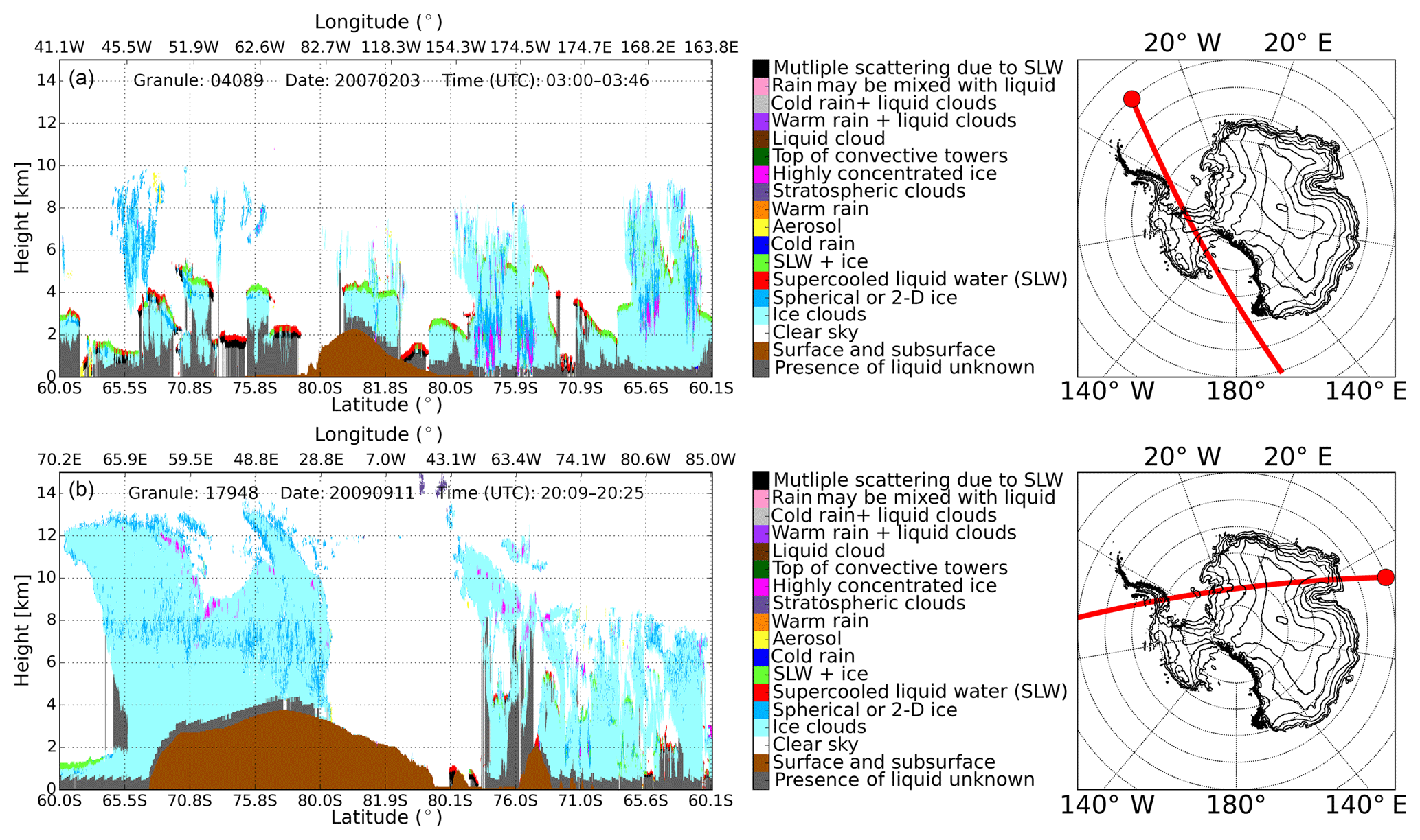
Figure 3Two examples of DARDAR-MASK transects (altitude vs. latitude and longitude) illustrating the various categorisation included in the DARDAR-MASK version 2. The summer transect (a) occurred on 3 February 2007, while the early spring one (b) occurred on 11 September 2009. The small map next to each transect shows the satellite track (solid red line) projected over the Antarctic region. The circle indicates the beginning of the tracks across the Antarctic.
As we are interested in mapping the occurrences of the liquid and the ice phase, we do not use the distinct categories developed for the ice phase but we consider all the ice categories together (namely the ice clouds, the highly concentrated ice and the spherical or 2-D ice). Hence we track the general ice phase occurrences (light blue, dark blue, purple of the colour-coded mask) and the occurrences of SLW wether it is mixed with ice (light green of the colour-coded mask) or not (red of the colour-coded mask). The vast majority of Antarctic tropospheric clouds occurs in these categories. Warm liquid cloud occurrence is observed on the margins of the domain (60–62∘ S; 100–180∘ W) in very negligible amounts compared to the rest of the investigated cloud phases.
Finally, note that the category “multiple scattering due to SLW” was not introduced in Ceccaldi et al. (2013) and was subsequently added by Ceccaldi (2014, their Sect. III.3.5). As explained in that work, this corresponds to the detection of a backscatter signal from below the SLW layer, which is still important despite a strong attenuation of the lidar signal there. If the radar does not detect any ice, this signal has to be caused by the multiple scattering in the layer of supercooled droplets above.
3.2 Methodology
3.2.1 Statistics
About 15 overpasses occur each day over the Antarctic region (Fig. 4a), which we define as the region poleward of 60∘ S. Following Adhikari et al. (2012) and Mioche et al. (2015), we divide the area into grid boxes of 2∘ in latitude and 5∘ in longitude, which correspond approximately to a grid box of 280 km by 220 km at 60∘ S and of 280 km by 80 km at 82∘ S (the southernmost latitude observed by the satellites). The grid, on which the overpasses are combined to derive the occurrence frequency of the clouds, appears in the maps of Fig. 4a and c. The shaded areas in Fig. 4d delimit the investigated Antarctic region in this study located between 60 and 82∘ S and the three different latitudinal bands used to derived latitudinally averaged vertical transects: the Southern Ocean (SO) transect (60–65∘ S), the coastal transect (65–75∘ S) and the interior transect (75–82∘ S).
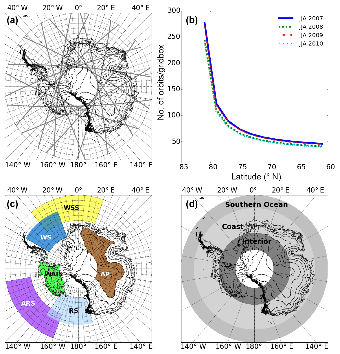
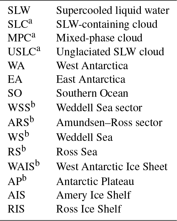
Figure 4(a) The Cloudsat tracks across the Antarctic on 1 January 2007, and the grid (grid boxes of 2∘ in latitude and 5∘ in longitude) used to derive the geographical distribution of cloud occurrences and extending between 60 and 82∘ S (b) The zonally averaged number of satellite overpasses per grid box as a function of latitude, for the whole winter season each year. (c) Areas of interest used in the study and introduced in Sect. 4.3 to investigate the monthly evolution of cloud occurrences. They are called WSS (in the Weddell Sea sector), ARS (in the Amundsen–Ross sector), WS (in the Weddell Sea), RS (in the Ross Sea), the WAIS (on the West Antarctic Ice Sheet) and AP (on the Antarctic Plateau). Names are recalled in Table 1. (d) The three latitudinal bands used for the average vertical transects presented in Sect. 4.2.
The sun-synchronous polar orbit of the satellites results in an exponentially increased sampling of the continent as we observe closer to the pole (Fig. 4b). The SO limit at 60∘ S shows one overpass every 2 days (∼45 per season) per grid box, while the southernmost limit at 82∘ S shows on average more than 2.5 overpasses per day (∼250 per season) per grid box. The sharp increase in the statistics towards the South Pole is welcome as it is the area where the cloud cover is the lowest (e.g. Bromwich et al., 2012). The measurement statistics hardly change along a given parallel due to the symmetry of the polar orbiters' trajectories in relation to the South Pole (hence the zonal average presented in Fig. 4b). The measurement statistics are very similar from one season and one year to the next. JJA is shown as an example in Fig. 4b. Only DJF 2010 shows a significant reduction (by 40 %) in the number of available DARDAR products. We use the 4 years 2007–2010 as they are the only 4 full years with night-time observations for the CPR, which works only by daylight due to a battery failure from 2011 onwards.
Note that despite the different times of satellite overpasses over the different Antarctic areas, we do not expect any diurnal cycle to bias our observations and conclusions. For instance, the local (UTC) times of the overpasses above the grid box including Rothera are 02:00 (05:00) and 17:00 (20:00), while for Halley they are on average at 01:30 (01:30) and 18:00 (18:00). The morning and evening times correspond to the descending and ascending nodes of the satellite overpasses. Cloud cover varies diurnally as a result of the development of convection, but in and around Antarctica this will be weak at all times of the year. Over the ocean, diurnal variation in the surface temperature is small. Even over the ice sheets, diurnally varying convective boundary layers develop in summer at locations like Dome C, but these layers are very shallow and do not generate convective cloud (King et al., 2006). Moreover, the ceilometer data introduced in Sect. 3.3 and used in Sect. 4.4.1 confirm the low amplitude of the cloud occurrence diurnal cycle (not shown) at Halley (2.5 % absolute variation) and Rothera (6 % absolute variation) compared to the average amplitude of the seasonal cycle (>20 %).
3.2.2 Cloud fraction mapping
Following Mioche et al. (2015) in their study of Arctic clouds with DARDAR v1 products, we derive a (temporal absolute) cloud fraction (or cloud occurrence frequency) Fcloud. It is the ratio of the number of cloud occurrences Ncloud per grid box over the number of observations (footprints) Nfootprints in that grid box: . A valid cloud occurrence is an occurrence of at least three adjacent vertical pixels flagged with the same condensed phase. We do not distinguish between precipitable and non-precipitable frozen hydrometeors as the ice phase includes both cloud ice and snow in the DARDAR products. We focus on tropospheric clouds, so that stratospheric features are not accounted for in the derived horizontal or vertical distributions of the cloud fraction. We use the tropopause height provided by the CALIOP product and stored in the DARDAR product. The tropopause lies at ∼9 km in the summer and at ∼12 km in the winter. The same method is used to derive the fraction FX of any given cloud type X (see below). This technique is applied for every month to derive a monthly averaged fraction in every single lat–lon grid box. To obtain the cloud (or any cloud type) seasonal fraction, the number of total occurrences of clouds (or any cloud type) over the 3 months of interest is divided by the total number of footprints in each grid box over these months. The relative fraction (as opposed to the previously defined absolute fraction) can also be computed for the different cloud types, where the number of observations Nfootprints is replaced by the number of cloud occurrences Ncloud in the ratio. In DJF (austral summer) of a given year, the month of December is the one from the previous year. For instance, DJF 2007 uses December 2006. Thus, we obtain maps of the geographical distribution of the cloud fractions. The vertical distribution of the cloud or any cloud type fraction is also computed by deriving the ratios as explained above but for each of the 60 m vertical pixels.
The fraction of SLW-containing clouds is called the SLC fraction, FSLC. Table 1 recalls the acronyms used for the various cloud types (as well as the ones for specific Antarctic regions). The DARDAR-MASK includes a mixed-phase category (“SLW with ice” – first type), and we extend this category by adding the clouds where a pure SLW layer is detected with at least three adjacent vertical pixels containing ice below (second type), following Mioche et al. (2015). In practice, most of the detected mixed-phase clouds are of the first type, but pure SLW layers with an ice phase immediately below are clearly detected. We interpret these as occurrences of a mixed phase since the ice below is immediately in contact with the liquid layer; their microphysics must be interacting. Note that cloud where ice crystals are too small and/or too few to be detected by the radar in the top SLW layer of the cloud is also possible (recall that in the upper atmosphere, for instance, the CPR cannot detect thin cirrus). A cloud top made out of SLW with ice precipitating below is characteristic of boundary layer mixed-phase clouds (e.g. Korolev et al., 2017) and, in practice, cloud layers flagged by DARDAR as actual mixed phase (and not pure SLW) come systematically along with ice below. The mixed-phase clouds (first and second types) are described by the MPC fraction, FMPC. Supercooled liquid-water-containing clouds (SLCs) that are not part of any mixed-phase clouds as defined above (hence being pure liquid) are categorised as unglaciated supercooled liquid clouds (USLCs), with a fraction of FUSLC. They are liquid clouds for which no glaciation process has occurred (see for example Fig. 3a: the layer appearing in red around 2 km altitude at longitudes between 51∘ W and 82∘ W). By “glaciation processes” we designate the processes by which a pure liquid layer becomes a mixed-phase layer. The SLC fraction will refer to any detection of SLW (whether involved in a mixed layer or not). Adding the USLC fraction and the MPC fraction gives the SLC fraction. An all-ice cloud category is defined and accounts for occurrences of the ice phase when no SLW at all is present in the investigated part of the troposphere (the whole of it or the low, middle or high part of it). This is proven to be useful to investigate occurrences of strict ice-only processes in order to put the behaviour of these clouds into perspective with SLCs. Importantly, all-ice and SLC fractions are complementary by definition. We can summarise all the fractions we are interested in and their relationships by writing the following:
Following Mioche et al. (2015), a distinction is made between low-level clouds (at altitudes between 500 m and 3 km above ground level), mid-level clouds (3–6 km above ground level) and high-level clouds (more than 6 km above ground level). When no restriction to a particular altitude level is considered, we will speak about the total cloud fraction or, simply, the cloud fraction. We choose to use ground level and not mean sea level as a reference for altitudes and, similarly, altitude levels rather than pressure levels in order to remain consistent in our description of clouds across the Antarctic region, where ground levels between 0 and 4 km above mean sea level are found. Using a mean sea level reference or pressure levels to discriminate between clouds of different height would artificially lead to an empty low-level cloud category as looking closer to the pole. Thus we do not make use of the International Satellite Cloud Climatology Project (ISCCP, Rossow and Schiffer, 1999) pressure levels (680 and 440 hPa, which approximately correspond to 3 and 6 km above mean sea level) as this was done for studies over the SO only. Our goal is to describe the marine and continental clouds of the Antarctic and their differences rather than comparing our observations to the numerous characterisations made over part of or the whole of the SO using A-Train (and sometimes DARDAR v1) and/or ISCCP observations (e.g. Hu et al., 2010; Haynes et al., 2011; Huang et al., 2012; Mason et al., 2014; Bodas-Salcedo et al., 2014; Huang et al., 2015).
3.2.3 Limitations of the products
Finally, two main limitations have to be considered when using space-borne lidar and radar data sets. First, the strong extinction of the lidar meeting a supercooled liquid layer prevents it from detecting any other liquid layer that could exist below this one. The lidar signal can also be extinguished closer to the surface because of optically thick ice clouds above. Figure 3a shows grey-shaded areas flagged “presence of liquid unknown”. This is illustrative of the lidar signal extinction below the detections of supercooled liquid layers (first part of the transect in Fig. 3a). This category is flagged in the mask when the lidar signal is extinguished and when at the same time the radar does not detect any ice. Second, the surface clutter or blind zone of the radar (Tanelli et al., 2008) (surface wave reflection blurring the signal) prevents it from detecting any ice cloud (or identifying the ice part of the MPC) close to the surface. This can be clearly seen when the identification of the ice phase ceases when nearing the ground (at ∼500 m above the surface) in Fig. 3a after the longitude 168∘ E and in Fig. 3b right at the beginning of the transect.
Practically, the clutter height is not constant, and it is flagged in the CloudSat products used to build the DARDAR-MASK products so that the latter does not take into account the radar signal in areas where the clutter is identified. This will result effectively in a reduced statistics close to the surface. The lidar information, however, is not filtered out. Hence, detection of supercooled liquid layers even in the blind zone of the radar can happen. To derive the geographical distribution of the cloud fraction we consider the atmosphere above 500 m above the surface, ignoring a large part of the radar signal ground contamination in order not to work with the very reduced radar or lidar statistics too close to the surface, following (Mioche et al., 2015). Their statistics was approximately halved (∼60 % loss) between 500 and 1000 m above the surface. In Appendix A we show vertical transects of the occurrence frequency of the lidar extinctions and the radar signal contamination (Fig. A1). Additionally, the monthly time series of the occurrences of radar signal contamination and lidar extinction or attenuation above 500 m above the surface are shown in Fig. A2. In our data set, ∼80 % of the radar observations are still available at an altitude of 500 m above the ground (Fig. A2a), and almost no contamination occurs above 1 km. Importantly, there is almost no seasonality in the radar clutter occurrences. Seasonality in the radar signal reflection can occur because of the changing nature of the surface (caused by more waves at the sea surface at a given time of the year Tanelli et al., 2008). The statistics of lidar observations show a ∼55 % occurrence in the signal extinction at 1 km above the surface and ∼65 % at 500 m above the surface (Fig. A2b). The lower altitude cut-off set at 500 m above the surface to derive the geographical distributions of the cloud fractions does not affect our conclusions, and this is discussed in Appendix B. It is mainly the absolute value of the USLC monthly fraction that is affected by this cut-off but not its relative variations (Fig. B1).
3.3 Ceilometer data set
Vaisala CT25k ceilometers were installed at Halley and Rothera in 2003, their purpose being to support logistical and scientific aircraft operations. They operate on the lidar principle, with a laser at 905 nm as a light source. The maximum measurement range of the instruments is 25 000 ft (∼7500 m) with a vertical range resolution of 15 m. In this study we use data sets from Rothera and Halley over 2007–2010 (Sect. 4.4.1). We use the operational products from the internal software of the instruments, providing the cloud base height. We do not use the complete backscatter signal. This requires specific processing (e.g. VanTricht et al., 2014), which is out of scope of the present study. The ceilometer allows different recording intervals (one measurement every 60, 30 or 15 s). Most of the time these settings were kept constant for years at one level or another, but there are also changes from one month to the next or even from day to day. Since we are looking at the ratio of cloud observation over the number of total observations, this is not an issue. Several cloud base heights are recorded if the instruments detects more than one cloud layer. However, the number of measurements when a clear second or third cloud layer is detected is negligible and we only used the first (lowest) detected cloud base height. For instance, at Rothera, 897 947 individual ceilometer measurements were recorded in 2007 and a first clear cloud base was detected in 400 589 cases (45 %). A second and third cloud layer with a clearly defined base height were recorded in 35 530 (4 %) and 1499 (0.2 %) cases, respectively.
The polar-optimised algorithm by VanTricht et al. (2014) effectively lowers the cloud base height by allowing for the detection of thin precipitating ice below the supercooled liquid layer at the top of the mixed-phase clouds. Since most of the cloud bases detected by the Vaisala's algorithm are already at a low level (see Sect. 4.4.1), in our particular case of (vertically integrated) low-level cloud cover comparisons between the ceilometers and DARDAR we cannot expect a significant change in using the VanTricht et al. (2014) algorithm. However, future work will certainly benefit from using the polar-optimised algorithm for characterising the vertical structure of clouds at these stations and improving the comparison between ceilometer and satellite detections.
4.1 Geographical and seasonal distribution of clouds and supercooled liquid water
The geographical distributions of the total cloud and SLC fractions are shown as seasonal averages derived over 2007–2010 in Fig. 5. They clearly show how the total SLC fraction distribution (Fig. 5e–h) differs from the total cloud fraction distribution (Fig. 5a–d). We first comment on the cloud fraction and then on the SLC fraction.
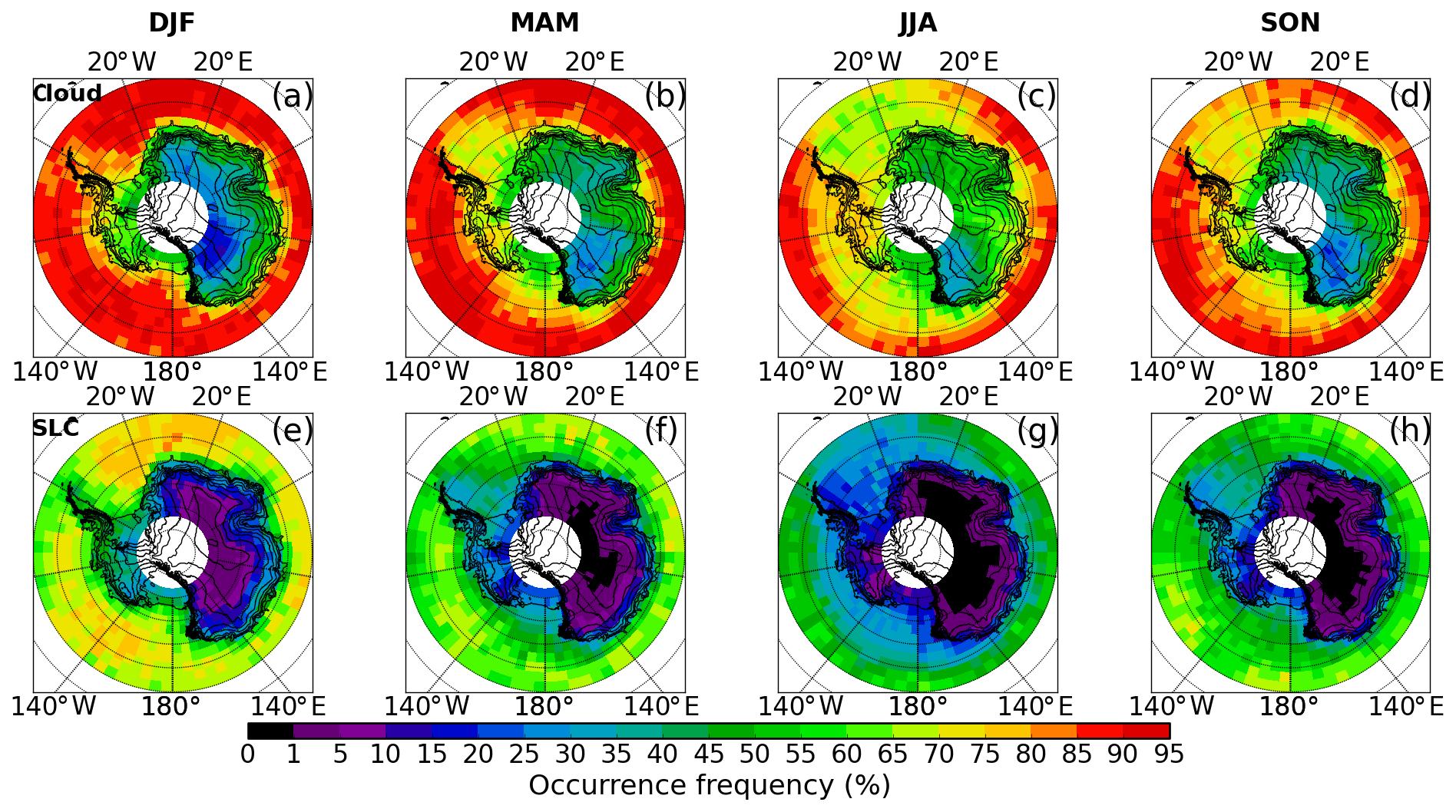
Figure 5Geographical distribution of the total cloud fraction (a–d) and the total SLC fraction (e–h) for each of the four seasons based on 2007–2010 averages.
Figure 5a–d show that the SO and the Antarctic seas have the largest cloud fractions as already demonstrated in previous studies using other synergetic A-Train products (Verlinden et al., 2011; Bromwich et al., 2012; Adhikari et al., 2012). There, the cloud fraction reaches values larger than 90 %. From summer to winter the cloud fraction decreases the most in the Weddell Sea and the Weddell Sea sector and in the Ross Sea (by an amplitude of ∼30 %). These are places where the sea ice formation extends the most equatorward (Fig. 2k). Observing the highest continental cloud fractions over the WAIS is consistent with the presence of the ASL to the north of it, which brings moisture from lower latitudes to the slopes of WA coasts. There, the orography induces adiabatic cooling and cloud formation (e.g. Scott et al., 2017). The deepening of the ASL in winter (Fig. 2c) is associated with an increase in the cloud fraction over the WAIS (Fig. 5c), which is consistent with the intense moisture fluxes and higher cloudiness related to the sustained cyclonic activity across the Amundsen and Ross seas (Nicolas and Bromwich, 2011), a process also observed along EA's coasts (Dufour et al., 2019).
A salient feature is the minimum of the cloud fraction reached over the megadune region (75–82∘ S, 110–150∘ E) (e.g. Frezzotti, 2002), west of the Transantarctic Mountains. In fact, the minimum cloud fraction occurs around 140∘ E longitude throughout the year. The largest value of this minimum occurs in winter (30 %–35 %). This region corresponds to the area with the largest subsidence of air on the plateau, as emphasised by Verlinden et al. (2011) (their Fig. 4). More generally, the lowest cloud fractions are found across the high-altitude terrain of the Antarctic Plateau, compared to the cloudier WAIS (by at least 20 % in absolute value). Outside of the megadune region, the cloud fraction in EA increases from 30 %–35 % in summer to 60 %–65 % in winter.
The SLC fraction geographical distribution (Fig. 5e–h) is in strong contrast to that of the cloud fraction, especially over the continent. In EA, the SLC fraction decreases sharply polewards and away from the coast in all seasons (Fig. 5e–h), following the increasing surface height. The SLC fraction is at most 10 % in summer over the plateau, decreasing to almost 0 % during other seasons and especially in winter. WA shows, in comparison to EA, larger continental SLC fractions in summer (30 %–40 % vs. 10 %–20 %). The SLC fractions are the largest over the ocean with an average value of ∼70 % (Fig. 5e). As for the cloud fraction, the strongest decrease in offshore SLC fractions in winter occurs in regions where sea ice forms. In summer, the eastern Weddell Sea and the Weddell Sea sector have the largest SLC fractions (75 %–80 %). The western Weddell Sea (60–40∘ W) shows systematically lower SLC fractions than the eastern Weddell Sea (40–20∘ W) and more particularly in summer, with a 12 % absolute difference in the SLC fraction (Fig. 5e).
To further emphasise the difference between cloud fraction distributions, we show the seasonal geographical distribution of the total all-ice, MPC and USLC fractions in Fig. 6. Recall that all-ice, MPC and USLC fractions describe – when added up – the entire cloud fraction (Eq. 1). By considering the all-ice fraction (Fig. 6a–d), we clearly highlight the enhancement of ice clouds over the WAIS from the summer season (20 %–25 %, Fig. 6a) to the winter season (∼65 %–70 %, Fig. 6c). This feature is explicable by the deepening of the ASL (Fig. 2c) and the upper-level low-pressure system in the Ross Sea region (Fig. 2g). The increase in the all-ice fraction in winter on the WAIS and in EA close to Princess Elizabeth Land (Fig. 1) near the coasts at ∼90∘ E is in agreement with the strengthening of the ASL and the other climatic low-pressure system located around 100∘ E (Fig. 2c) and drives the increase in the cloud fraction (Fig. 5c).
The all-ice fraction distribution in winter (Fig. 6c) ranges between 45 % and 70 % across the whole continent, except west of the Transantarctic Mountains, where it is around 30 %. It is interesting to note that the cloud-depleted area observed in the cloud fraction over the megadune region is observed in the all-ice fraction throughout the year but not in the SLC fraction. This area is located downwind of the ASL (the upwind area being Marie Byrd Land, Fig. 4a) and of the upper-level low-pressure system of the RIS. The airstream of the ASL will meet with the Transantarctic Mountains and prevent moisture or cloudiness from progressing further.
West and east of the Amery Ice Shelf (AIS, Fig. 1), the all-ice fraction is larger than over it. At the same time the SLC fraction is actually larger over the AIS than in the neighbouring areas of similar latitudes. This can be seen in all seasons. This is consistent with the presence of the depression in the land south of the AIS, where the absence of a sharp longitudinal gradient in the orography would allow (due to the lack of adiabatic cooling) for slower or delayed cooling and the liquid phase not to freeze.
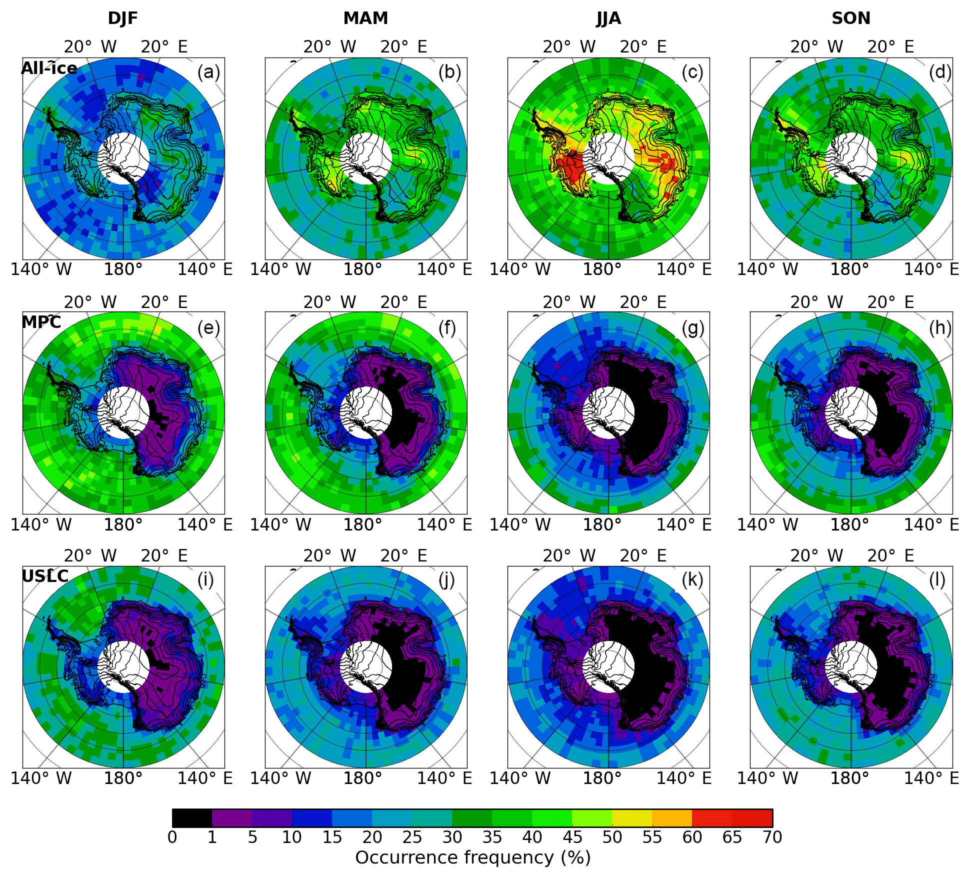
Figure 6Geographical distribution of the total all-ice cloud fraction (a–d), MPC fraction (e–h) and USLC fraction (i–l) for each of the four seasons based on 2007–2010 averages.
The largest all-ice fractions each season happen to be where the orography is and southwards of places where the three climatic low-pressure systems are (see Sect. 2, and Fig. 2a–d). Hence, the all-ice fraction corresponds to orographic clouds and fewer of those clouds occur over the large Weddell and Ross sea embayments (e.g. Fig. 5e). The Antarctic Peninsula (∼65∘ W) also acts as a barrier to the dominant westerlies and triggers ice cloud formation through interaction between the airflow and the orography. The all-ice fraction is larger in that region than in areas over water nearby at similar latitudes. It can be already noticed that the spatial pattern of the sea ice fraction spatial distribution in winter is not similar to that of the all-ice cloud fraction distribution, contrary to what is observed for the SLC fraction (for instance, compare the winter patterns of sea ice in Fig. 2o with the winter cloud and SLC distributions in Fig. 5c and g on one side and the winter all-ice distribution in Fig. 6c on the other side).
The MPC fraction (Fig. 6e–h) and the USLC fraction (Fig. 6i–l) are the largest in summer. There is an area of concentrated higher USLC fraction in the eastern Weddell Sea in summer, which has no counterpart elsewhere in the Antarctic region (e.g. in the Ross Sea). Over the SO and the seas, the absolute difference between the average MPC fraction and USLC fraction is the largest in autumn (33 % vs. 20 %, Fig. 6f and j), while it is the smallest in spring (26 % vs. 23 %, Fig. 6h and l). This difference is 8 % in summer and 4 % in winter. As for the SLC fraction, the MPC and USLC fractions are lower on the continent and particularly in EA, where they decrease polewards. Interestingly, these fractions show no significant differences between each other on the continent, in contrast to what is observed over seas. This will be investigated and discussed further below.
4.2 Vertical distribution of clouds and supercooled liquid water
As a complement to the geographical distribution of clouds, we now investigate their vertical distribution with a focus on the SLW. We show the 4-year average transects (at the 60 m vertical resolution) in the three latitudinal bands defined in Fig. 4d, aimed at roughly describing the SO (60–65∘ S), the coastal areas (65–75∘ S) and the interior of the continent (75–82∘ S). Transects were built for the cloud fraction (Fig. 7a), the SLC fraction (Fig. 7b), the MPC fraction (Fig. 8a) and the USLC fraction (Fig. 8b). In Fig. 8, isotherms built using the ECMWF temperatures stored in the DARDAR product indicate the average temperature at which MPCs and USLCs form. Similar transects of the cloud fraction as the ones shown in Fig. 7 are discussed in Adhikari et al. (2012) for 2007–2010 and in Verlinden et al. (2011) for 2007–2009. However, we show the 4-year average for the cloud fraction to put the other transects into context. We limit ourselves to the low and middle altitudes as this is where all SLC form. The average topography in each transect is indicated by the solid white line. Since the topography is not homogeneous along any given meridian within each latitudinal band, the number of effective footprints per altitude level will change along any meridian in the coastal and the interior transects. In order to show a smooth pattern of cloud vertical distribution we divide the number of occurrences of any cloud type in any three-dimensional grid box by the effective number of footprints in it (this number equals the number of overpasses above that grid box if the grid box is above the surface, and zero, if it is below the surface). In doing so, when averaging to build the transect, we account for the actual reduction in footprints along each meridian at altitude levels that are partly above and partly below the surface. Note that, since the fractions are derived in each of the 60 m vertical bins, they are lower than the ones derived for the geographical distributions, for which the occurrences of clouds were derived over the tropospheric column whatever their altitude.
The reduced statistics due to the radar blind zone and the lidar signal extinction across the Antarctic clearly appears in the resulting transects for the cloud fraction at ∼500 m a.s.l. (e.g. Fig. 7Aa). This is illustrated and discussed in Appendix A with Fig. A1. There is a sharp reduction in the low-level cloud fraction below ∼500 m a.s.l., which corresponds to the lesser ability to detect clouds because of the radar blind zone. Satisfyingly, despite a reduction by up to 40 % of the number of valid radar observations from 1 km to 500 m a.s.l. (Fig. A1a), no discontinuity appears in the vertical transects above 500 m a.s.l. (Fig. 7Aa). This suggests that the vertical distribution of cloud fraction is well reproduced above this altitude and that it is legitimate to use 500 m as a lower-altitude cut-off for the geographical distributions introduced in the previous section.
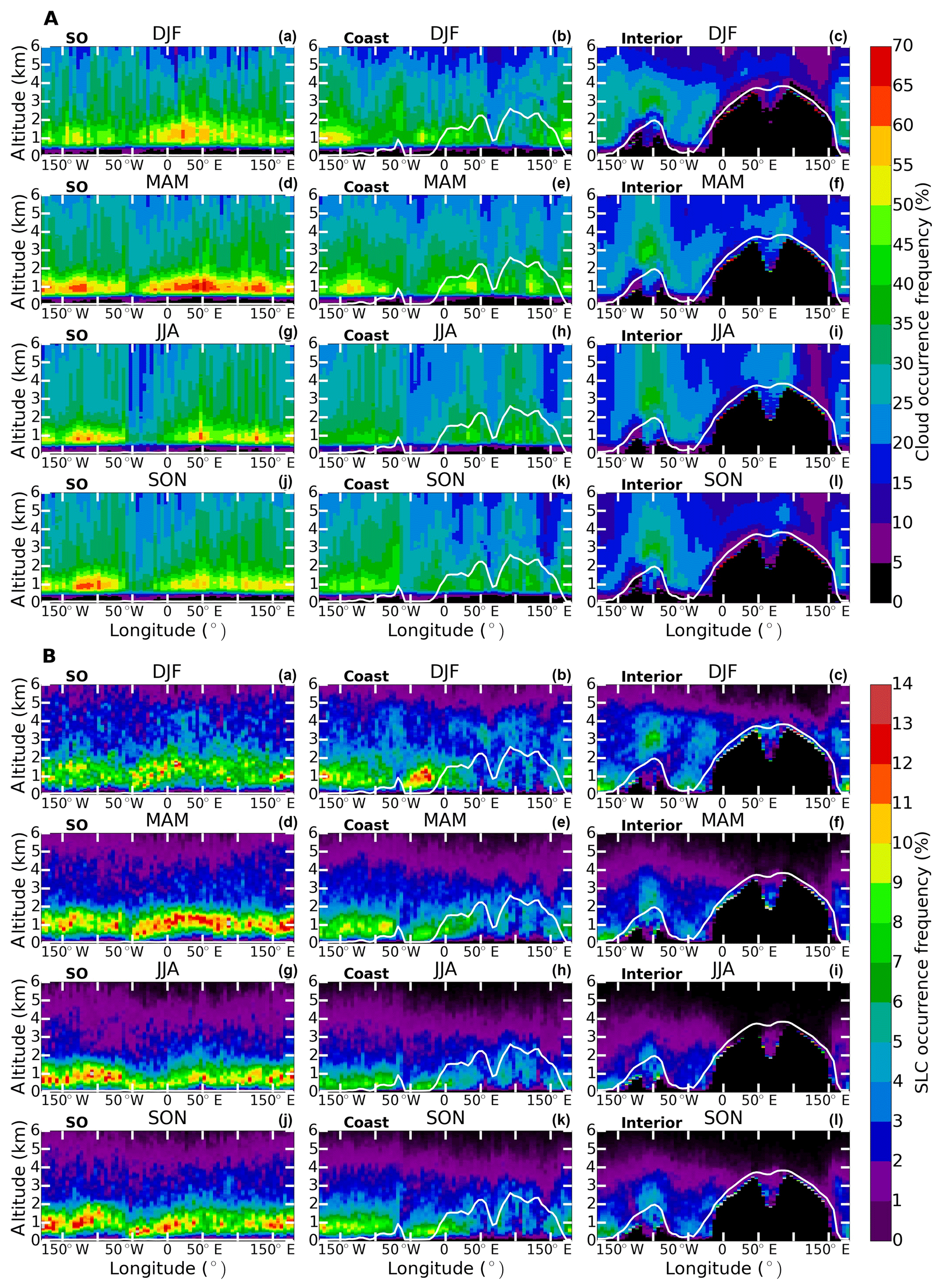
Figure 7(A) Four-year (2007–2010) average seasonal vertical transects of the cloud fraction, spatially averaged over three latitudinal bands defined in Fig. 4d (SO stands for Southern Ocean). One column corresponds to one latitudinal band, showing the four seasons. Each line corresponds to one season. (B) Same as (A) for the SLC fraction. The white line is the average surface elevation in the latitudinal band.

Figure 8(A) Same as Fig. 7A but for the MPC fraction. (B) Same as (A) but for the USLC fraction. Additionally, isotherms are shown every 5 ∘C (dotted white lines) and they are labelled but ignore the minus sign in the temperature value. The warmest temperature shown in all panels is −5 ∘C. In plots (Aa) to (Ak) and (Ba) to (Bk) (SO and coastal transects) isotherms are shown down to −25 ∘C only, while for the interior transects they are shown down to −35 ∘C.
4.2.1 Cloud vertical distribution
The highest vertical cloud fractions (70 %) occur at low altitudes in the SO transects (Fig. 7Aa, d, g and j). The maximum of the summer cloud fraction occurs across the boundary between the Weddell Sea sector and the Indian sector (20∘ E) and in autumn in the Indian sector and the Amundsen–Ross sector (Fig. 7Aa and d). In spring, the latter has the highest occurrences of low-level clouds. To the east of the Antarctic Peninsula (∼65∘ W, hereafter called the peninsula), north of and in the Weddell Sea (60–25∘ W), the cloud fraction is halved at each altitude level between 0.5 and 2 km a.s.l. in winter (20 %–30 % Fig. 7Ag and h) compared to summer (40 %–60 % Fig. 7Aa and b). This reduction is less pronounced above 2 km a.s.l. To the west of the peninsula, the cloud fraction is hardly changed at similar altitudes. Hence, this drop in the cloud fraction induces a dramatic difference in the winter and spring longitudinal distributions of low-level clouds across the peninsula, between the west (45 %–55 %) and the east (20 %–30 %) of the mountain chain. Additionally, and whatever the season (Fig. 7b, e, h and k), there is a ∼20 % absolute difference in the mid-level cloud fractions between both sides of the peninsula, i.e. well above the highest peak of the peninsula (∼2.5 km). East of the peninsula, the lowest low-level cloud fractions in winter and spring coincide with the largest sea ice fractions (Fig. 4k and l).
In EA, east of the AIS (around 90–100∘ E, Fig. 7Ah) a local increase in the vertical extension of coastal cloud fraction occurs in winter, at altitudes up to 6 km a.s.l. This feature in the vertical distribution of clouds occurs while the climatic low-pressure system located off the coast is strengthened (Fig. 4c). This low-pressure system is the weakest in summer (Fig. 4a), and the cloud fraction is also at its lowest (∼25 %) (Fig. 7Ab). This seasonal variation is seen during each year taken separately. South of the AIS (∼70∘ E), the cloud fraction is lower than immediately to the east and to the west of the AIS (Fig. 7Ae, h and k). This is the effect of the land depression there, preventing the orographically induced cloud formation from occurring.
Generally, the cloud vertical extension follows the air mass interactions with the coastal topography. This is also clearly visible in the interior transects (Fig. 7Ac, f, i and l) around 100∘ W, on the WAIS. There, the ASL brings moisture from lower latitudes, triggering cloud formation through adiabatic cooling on the steep coasts. In winter the vertical extension of clouds lead to values of 45 % and 30 % at 2 km and 6 km a.s.l. against 40 % and 10 % in summer. Hence, higher clouds occur at higher altitudes in winter and this is consistent with the deeper ASL and the contraction of the westerly circulation towards the coast (Fig. 4c). In EA, the area of lowest cloud fraction (∼5 %–10 %) is visible around 140∘ E consistently with observations made by Verlinden et al. (2011) over 2007–2009. It is the area of largest subsidence and also immediately west of the Transantarctic Mountains, which prevents moisture or cloudiness from WA entering EA. The land depression extending poleward from the AIS is the area of maximum cloud fraction in the interior in winter (∼70∘ E, Fig. 7Ac, f, i).
4.2.2 Supercooled liquid-water vertical distribution
The largest SLC fractions are consistently found in the lowest (warmest) atmospheric layers, below 2 km altitude in the Southern Ocean transect (Fig. 7Ba, d, g, and j) and the coastal regions (Fig. 7Bb, e, h, and k). The largest SLC fractions over the largest oceanic area are found in autumn across the Weddell Sea sector and the Indian sector (0–70∘ E) at 1–1.5 km altitude (Fig. 7Bd). This corresponds to an area of preferred MPC formation compared to USLCs (compare transects Fig. 8Ad and Bd). In the coastal transect the Weddell Sea is an area of enhanced SLC formation (60–25∘ W, Fig. 7Bb). This maximum is principally due to the increase in the USLC fraction there (Fig. 8Bb) rather than to the MPC fraction (Fig. 8Ab). This already appeared in the USLC fraction geographical distribution (Fig. 6i). This suggests that the Weddell Sea is an area more prone to maintain layers of supercooled liquid with no significant glaciation process. There is a clear cut in the SO zonal distribution of the SLC fractions at the northern tip of the peninsula (∼60∘ W), causing an asymmetry in this distribution. Lower altitudes (a.s.l.) are reached by SLCs to the east of the peninsula compared to the west. This is particularly visible outside summer months (Fig. 7Bd, g, and j) and can be explained by the lower surface temperatures on the eastern side of the peninsula, which is well documented in the literature (e.g. Morris and Vaughan, 2003). Also note the changes in the isotherms, which have lower altitudes to the east of the peninsula (Fig. 8Aa, d, g and j).
Over water, the largest USLC fractions generally occur between 0.5 km and 1 km a.s.l., and the largest vertical extent of the largest USLC fractions occurs in the Weddell Sea (Fig. 8Bb). The maximum MPC fractions are located between 1 km and 1.5 km a.s.l. with no MPCs detected below 500 m a.s.l. The isotherms indicate the average temperatures at which MPCs and USLCs form. In the SO transect and in the coastal transect, the largest MPC fractions occur between −15 and −5 ∘C and more particularly between −15 and −10 ∘C. In the SO transect, USLCs occur at temperatures above −5 ∘C in summer (Fig. 8Ba) and between −10 and −5 ∘C in other seasons (Fig. 8Bd, g and j). The high USLC fractions in the Weddell Sea in summer between 0.5 km and 1 km a.s.l. occur at temperatures between −10 and −5 ∘C (Fig. 8Bb).
In the interior transects, the SLC fraction is the largest above the WAIS (∼100∘ W) and the RIS (170∘ E–150∘ W) throughout the year (Fig. 7Bc, f, i, and l). In EA, on the plateau, SLCs occur almost exclusively in summer at temperatures down to −35 ∘C. The SLC fraction maximises in summer at 3 km a.s.l. over the WAIS and below 500 m a.s.l. above the RIS (Fig. 7Bc), mainly in the form of USLCs (compare Fig. 8Bc and Ac). Over the WAIS, this maximum occurs at average temperatures between −23 ∘C and −20 ∘C (Fig. 8Bc) and around −25 ∘C in other seasons. It is reminiscent of quasi-steady-state mountain-wave orographic clouds displaying supercooled droplets down to −33 ∘C with no ice (Heymsfield and Miloshevich, 1993). However, satellite observations do not allow a statement to be made on the lifetime of such a feature. Note that low-level SLCs that are categorised as USLCs in the radar blind zone above the RIS (below 500 m a.s.l.) could actually be MPCs. Silber et al. (2018), who investigated liquid-bearing clouds with ground-based measurements at McMurdo Station (167∘ E) at the edge of the RIS throughout the year 2016 did not differentiate between pure and mixed SLC layers. Thus, we cannot determine the preferred formation of USLCs or MPCs at very low altitudes there. In EA, the presence of SLCs is evidenced in summer (Fig. 7Bc), while no SLCs are detected over the plateau in winter, except where the depression of the land south of the AIS is (Fig. 7Bi). There, poleward intrusion of moisture and cloudiness from the coastal areas would cause enhanced SLC fractions (Fig. 7Ai).
Unlike for the cloud fraction, no discontinuity occurs in the SLC fraction vertical distribution close to the surface, especially over seas (Fig. 7B). This suggests that the statistics of the SLC fraction vertical distribution close to the surface is not much affected by the reduced statistics due to the lidar extinctions (∼80 % near the surface, Fig. A1d). Above land, some spurious SLC fraction enhancements appear at the surface on very rare occasions, though (e.g. Fig. 7Bc, at ∼50∘ E). It is also interesting to note that the maximum in the vertical MPC fraction occurs above 1 km height above ground level in the transects (Fig. 8A), suggesting that the decrease in MPC occurrences below 1 km is rather real and not an artefact of the 40 % reduced statistics (at 500 m a.s.l.) caused by the radar blind zone. The consequence of this is that the picture given by the DARDAR-MASK products of the MPC fraction and the USLC fraction is representative of their actual averaged distribution down to 500 m a.s.l. and possibly down to the surface for the SLC fraction at least (which does not rely on the radar signal). Hence, using a 500 m lower altitude cut-off for deriving the distributions of MPC and USLC fractions seems legitimate despite the reduced statistics.
4.3 Monthly time series over specific Antarctic regions
4.3.1 Total cloud and phase fractions
We now spatially average the geographical distribution of the total cloud fractions presented in Sect. 4.1 over distinct areas defined in Fig. 4c. In doing so, we increase the statistics compared to a single grid box, while we pin down the monthly evolution in these regions. The geographical areas investigated are called WSS (in the Weddell Sea sector), ARS (in the Amundsen–Ross sector), WS (in the Weddell Sea), RS (in the Ross Sea), AP (the Antarctic Plateau) and the WAIS (Fig. 4c and Table 1). We also show the monthly time series for the whole Antarctic region (60–82∘ S). Note that ARS and WSS are of similar sizes, as WS and RS. Figure 9 shows the monthly evolution of several total fractions: cloud (a), SLC (b), all-ice (c), MPC (d) and USLC (e). The shaded areas indicate the 4-year maximum and minimum monthly average values as an indication of the amplitude of interannual variability.
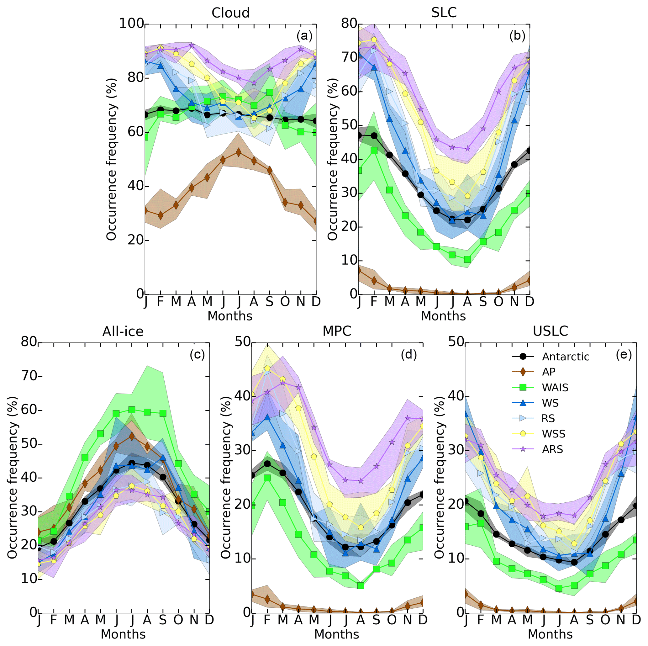
Figure 9Four-year (2007–2010) average monthly time series of the total cloud fraction (a), SLC fraction (b), all-ice fraction (c), MPC fraction (d), and USLC fraction (e). See Sect. 3.2 for the definition of the cloud categories. The different colours correspond to the different investigated regions (see map in Fig. 4c): WSS (in the Weddell Sea sector), ARS (for the Amundsen–Ross sector), WS (in the Weddell Sea), RS (in the Ross Sea), the WAIS (on the West Antarctic Ice Sheet) and AP (Antarctic Plateau). The shaded areas indicate the amplitude between the monthly minimum and maximum encountered over the years from 2007 to 2010.
A striking feature is the constant average cloud fraction throughout the year for the whole Antarctic region, around 68 % (black lines in Fig. 9) (Fig. 9a). When considering specific regions, different patterns appear. Generally, the maximum cloud fraction over continental regions occurs in winter and the minimum in summer, while the opposite occurs over oceanic regions. The cloud fraction derived for ARS shows the lowest amplitude of variation. It decreases from 90 % to 92 % in mid-autumn and throughout the winter and reaches a minimum of 78 % by the end of it. It increases again, reaching a second maximum around 90 % in late spring. A similar pattern appears for WSS, with a stronger decrease throughout winter, down to 65 %. This is consistent with the larger sea ice fractions observed in that area in JJA (Fig. 2o) and SON (Fig. 2p) and can be related to the likely reduced moisture flux into the atmosphere. WS and RS show the same pattern of a decreasing cloud fraction, starting from a maximum in summer. However, the cloud fractions are on average lower in winter over RS (∼60 %) than over WS (∼70 %). On the continent, the WAIS shows a slight increase in cloud fraction from summer (60 %) to winter (75 %) before decreasing abruptly from September to October. A much clearer trend emerges over the AP with a steady increase in cloud fraction from summer to winter and a maximum in July. It is the area where the seasonal cycle has the largest amplitude of variation (as already noted by Verlinden et al., 2011, using vertical transects). The same abrupt decrease in the cloud fraction as over the WAIS is noticeable between September and October.
The monthly evolution of the SLC fraction (Fig. 9b) is a general decrease from summer to winter with a minimum reached in August, before increasing again. This seasonal cycle is not biased by one of the lidar signal extinctions, which has occurrences that are equal to or lower than the SLC occurrences and follow the same pattern (Appendix A, Fig. A2). As a lidar signal extinction will happen below a SLC detection, this is expected. Some of the SLCs may be detected just above the 500 m lower altitude cut-off, so that the SLC occurrence is then counted, but the extinguished area below is missed in the statistics. Extinction or attenuation of the lidar signal can also happen because of optically thick ice clouds, and this is why the occurrences of extinctions and attenuations are almost as important in the winter as they are in the summer over the WAIS (Fig. A2). Overall, the seasonal cycle of the SLC fraction above 500 m above the surface is not biased by the lidar extinctions. The largest SLC fractions occur in ARS and WSS (both 75 %) in summer against 40 % and 30 % in winter. The lowest values of the SLC fraction are observed above the continental areas. The SLC fraction in the WAIS is 40 % in summer and 10 % in winter. The plateau has few but non-negligible SLC occurrences, with ∼10 % in January, and none by the end of winter and early spring. The relatively simple SLC fraction seasonal cycle points to the temperature seasonality as being one of the main drivers everywhere in the Antarctic (colder temperatures favour more glaciation in clouds).
Contrary to the cloud fraction evolution, the all-ice cloud fraction shows the same evolution over each area, increasing from the end of the summer to the winter (Fig. 9c). ARS and WSS show similar values ranging from 15 % to 35 %, while the WAIS reaches the largest 4-year average of 60 %. The AP has the second largest values of all-ice fractions in winter (50 %). This fraction is lower than in the WAIS and can be explained by the ASL located off the WAIS coast, contributing to a direct inflow of moisture (and cloudiness). Note the almost identical evolution for the cloud and all-ice fractions over the AP, showing the almost exclusive presence of ice clouds there. These fractions only differ during the summer months, when SLC fractions are not negligible (∼10 %, Fig. 9b).
A striking difference appears between the MPC and the USLC fractions (Fig. 9d and e) when considering the transition from beginning of summer to autumn. All regions – with the exception of the AP – show a local maximum of the MPC fraction in late summer or early autumn before a decrease in the following months, with a minimum reached around August. Conversely, the USLC fraction shows a steep decrease over the same period, which starts in January. This difference suggests that the glaciation process converting the supercooled liquid to a mixed phase follows a distinctly different cycle from the one describing the mere occurrence of supercooled liquid (although the former is obviously related to the latter). These differing behaviours are readily observed by comparing the Antarctic averages (solid black lines) in Fig. 9d and e. The differences in MPC fractions between marine areas (ARS, WSS, WS and RS) are larger than the differences in the USLC fraction between the same areas. For instance the USLC fractions are within a 5 % range of values except during winter (8 %), while the MPC fractions can differ by more than 15 %. This points to larger regional differences in the glaciation process (and occurrences of MPC) than in the mere occurrences of USLCs.
4.3.2 Cloud and phase fractions at low, middle and high levels
To look further into the details of the monthly evolution of the different cloud fractions, we divide them into low-level, mid-level and high-level fractions, as defined in Sect. 3.2. Figure 10 shows the all-ice fractions (a–c), the SLC fractions (d–f) and the MPC fraction (g–i). Since the addition of the all-ice and the SLC fractions gives the cloud fraction, it is easy to infer what the dominant component of the cloud fraction is and we do not show the cloud fraction here, although we still refer to it.
Over the continent, the monthly variability of the cloud fraction is primarily driven by the mid-level and high-level all-ice clouds (Fig. 10b and c). The monthly variability is within a 30 % range and 35 % range for mid- and high-level all-ice fractions on the WAIS, and 30 % and 15 % over the AP. Regarding the AP, the mid-level clouds can virtually be considered high clouds (in comparison to the oceanic regions) since the average altitude of the plateau is 3 km a.s.l. The evolution of the continental mid-level and high-level all-ice cloud fractions appears to be the same in both WAIS and AP, changing from a minimum in summer to a maximum in winter. This is consistent with the increases in cyclogenesis and depressions offshore in that season (e.g. King and Turner, 1997), leading to more intrusions of weather systems over the continent. The monthly evolution of continental clouds is essentially driven by the all-ice clouds. The mid- and high-level clouds detected over the WAIS and the AP are almost exclusively of the all-ice type given the much smaller mid-level SLC fractions (0 % and ≤10 % for AP and WAIS) compared to the mid-level all-ice fractions (20 %–50 % and 10 %–40 % for AP and WAIS) on one side and the almost null high-level SLC fraction (except over ARS) compared to the all-ice fractions on the other side.
Interestingly, over water (WS, RS, WSS and ARS regions) the mid-level cloud fraction shows almost no monthly variability compared to the low-level cloud fraction and the high-level cloud fraction (not shown). Mid-level cloud fractions are always within a 10 % range of values in ARS, WSS, RS and WS. We can understand the absence of monthly variation for mid-level cloud fractions over marine areas, since the ∼13 % increase in mid-level all-ice fraction (Fig. 10b) is almost compensated by a similar decrease in the SLC fraction (∼10 % decrease, Fig. 10e). This may be explained by the mid-level liquid phase being more often converted or replaced by ice in the winter season. Over water, the low-level cloud fractions are within a ∼40 % range of values in WS, ∼30 % in RS, ∼35 % in WSS and ∼20 % in ARS and this variability is caused by the SLC fraction (Fig. 10d). High-level cloud fractions are driven by the all-ice fraction and are within a ∼25 % range of values in WS, ∼15 % in ARS and WSS, and ∼10 % in RS. This demonstrates that the variability of the cloud fractions over water is firstly due to the low-level liquid-bearing clouds, which dominate the cloud fraction, and secondly to the high-level all-ice clouds, while mid-level clouds have little influence. Over marine regions (WS, RS, WSS, ARS), the monthly variability of the all-ice fraction (Fig. 10a–c) is largely driven by the mid- and high-level all-ice clouds (Fig. 9b and c), pointing to the increased cyclonic activity and number of frontal systems in winter (as for the general cloud fraction).

Figure 10(a–c) Four-year (2007–2010) average monthly time series of the low (a), middle (b) and high-level (c) all-ice fraction for the different Antarctic regions defined in Fig. 4c. (d–f) Same as top row but for the SLC fraction. (g–i) Same as top row but for the MPC fraction.
The monthly evolution of the low-level MPC fraction clearly differs from the low-level all-ice fraction, but also from the low-level SLC fraction. Over marine areas, little monthly variation in the low-level all-ice fraction occurs throughout the year in comparison to the low-level MPC fraction, suggesting that different factors affect their respective formation and evolution. More particularly, the monthly variation observed for the low-level all-ice fraction in WS, WSS and ARS is in a range of values of 5 % (10 % for RS), while the monthly variations in low-level MPC fractions are within a larger range of values, i.e. 20 % for WSS, 15 % for WS and RS, and 10 % for ARS. The largest part of the total USLC fraction is driven by the low-level USLCs (not shown), which does not show a local maximum at the end of summer or beginning of autumn, explaining the different patterns between the low-level SLC (Fig. 10d) and MPC (Fig. 10g) seasonal cycles. Finally, Fig. 10g demonstrates that the singular evolution of the MPC fraction from summer to autumn (Fig. 9d) is due to the low-level MPC. The mid-level MPC fraction does not display any similar local maximum in autumn. The particular monthly variation in the low-level MPC fractions points to a seasonal cycle of the glaciation process, involving interactions with the surface and/or the lowest layers of the troposphere. Note that, given the absence of seasonality in the radar clutter occurrences (Fig. A2), identifying ice in SLCs to assess the existence of a mixed-phase cloud seasonality is not biased.
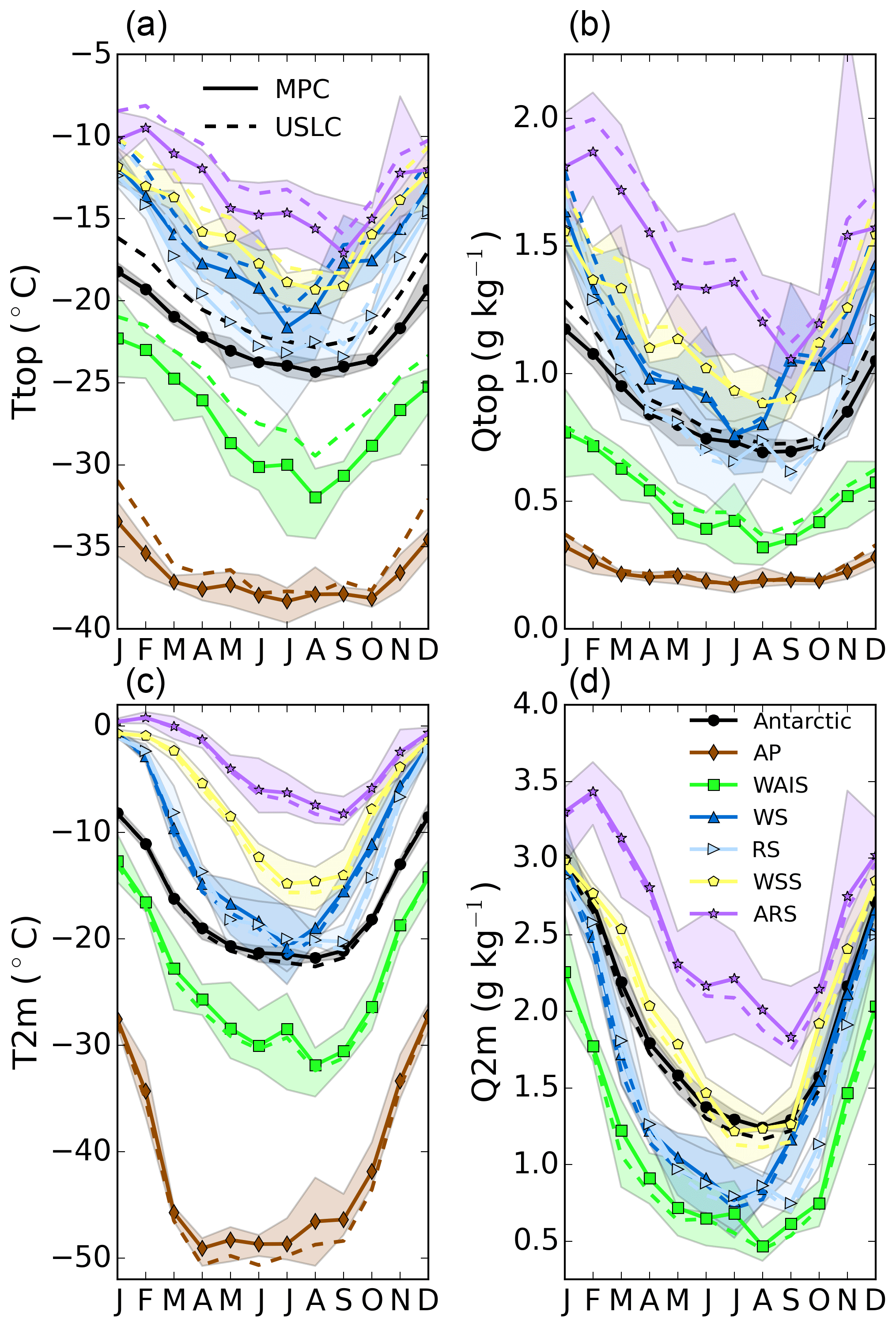
Figure 11(a–b) Monthly time series of the in-cloud temperature (Ttop) (a), and of the in-cloud water vapour mixing ratio (Qtop) (b), at the top of the low-level MPC and USLC layers, for the different regions of interest. (c–d) Monthly time series of near-surface (2 m) temperature (c) and the water vapour mass mixing ratio (d) below these layers. The shaded areas indicate the interannual variability for the MPC layers. For readability, the ones for the USLC layers are not shown, but they are of similar amplitude.
Figure 11 shows the monthly time series of the in-cloud temperature and water vapour mass mixing ratio at the top (Ttop and Qtop) of the low-level MPCs and USLCs, as well as the ones at the surface (T2m and Q2m) below where these clouds occur. The seasonal cycles of Ttop and T2m show a similar pattern to that of the SLC fraction suggesting the temperature as being the main driver of the SLC fraction evolution. The decrease in Qtop and Q2m is a direct consequence of the formation of sea ice and the reduction in moisture coming from the sea surface. Ttop of USLCs are larger than those of the MPC layers as the latter form at higher altitudes on average and have some active glaciation process suggestive of these lower temperatures. Note that, in the DARDAR-MASK, the two criteria using temperature in the identification of supercooled liquid is −40 ∘C, taken as the homogeneous nucleation temperature, below which the lidar backscatter will be considered to come from highly concentrated small ice crystals, and 0 ∘C, above which the liquid layer will be considered warm liquid (Ceccaldi et al., 2013). Apart from that it is the combination of lidar and radar observations that determines whether or not liquid and ice are simultaneously present. Hence, our observations of systematic higher average temperatures (and lower altitude – from Sect. 4.2) of the USLC are, while being independent, in line with the identification of these layers. Marine SLC top temperatures range between −22 and −10 ∘C. Continental SLC top temperatures range between −38 and −22 ∘C. The average lowest SLC top temperature occurs on the plateau (−35 in summer and −38∘ in winter). The statistics based on the highest number of samples, i.e. those for the whole Antarctic region (black lines in Fig. 11a), give a 1.5–2 ∘C warmer Ttop for USLCs than for MPCs. This temperature difference is significant at the 99.9 % level (using a t test), while the differences between Qtop for MPCs and USLCs is significant at the 90 % level only. There are no statistically significant Antarctic-wide differences in the near-surface temperature and water vapour mixing ratio between the MPCs and USLCs (Fig. 11c and d). This shows that the average near-surface conditions are the same for both types of SLC and more particularly over water. The only exception is the winter near-surface temperature on the plateau, which corresponds to extremely low and almost null SLC occurrences (Fig. 10g and j).
4.4 Comparison with ground-based measurements from the coast to the interior
The DARDAR products were validated in the Arctic by Mioche et al. (2015) using comparisons with a ground-based micropulse lidar. In this section we use the geographical cloud fraction distributions derived above to make comparisons with ground-based measurements of different sorts (cloud fraction, precipitation, SLC fraction) taken over 2007–2010 in Antarctica.
4.4.1 Ceilometer cloud base observations at Rothera and Halley between 2007 and 2010
In order to get a better perspective of the monthly evolution of cloud fraction illustrated by Fig. 9a, we performed qualitative comparisons with ceilometer data collected at the British Antarctic Survey's stations Rothera and Halley (Fig. 1) for the period 2007–2010. These were introduced in Sect. 3.3. We compare these with our low-level cloud fraction as the average height of cloud bases detected by the ceilometers is ∼1600 m at Rothera and ∼1000 m at Halley. When using the data from the ceilometers, we plot cloud base occurrences as measured starting from above the surface (>0 m) and from above 500 m above the surface (>500 m). In order to have enough monthly statistics from the satellite overpasses we extend the analyses to larger regions than the grid box containing the respective station (see Fig. 4a). Hence, in addition to the stations' grid boxes we derive the low-level cloud fraction using – for Rothera Station – the Bellingshausen sea (i.e. upwind of the station) and – for Halley – the Weddell Sea (off the Brunt Ice Shelf where Halley sits). From Fig. 5a–d, both station grid boxes experience similar seasonal cloud fractions to the one from these nearby areas. Thus it is legitimate to use those larger areas as proxies for both stations. Rothera is on the lee side of Adelaide Island's mountains, though, meaning that part of the clouds observed over Rothera are orographic in nature and that local effects should be more pregnant than at Halley.
Figure 12a shows the monthly evolution of the low-level cloud fraction derived for the grid boxes corresponding to Rothera (triangles) and Halley (circles) using solid lines, as well as for the Bellingshausen Sea and the Weddell Sea using dotted lines. Figure 12b shows the cloud fraction restrained to and not restrained to ceilometer detections above 500 m above the surface for both stations (using the same distinct markers as for Fig. 12a). In each figure the shaded area indicates the maximum and the minimum monthly average over the 4 years (the interannual variability). The monthly evolution of fog occurrences (reported in the ceilometer data set as “full obscuration but no cloud base detected”) is also reported for both stations.

Figure 12(a) Four-year (2007–2010) average time series of the monthly mean low-level cloud fraction plotted for the grid box corresponding to Rothera (triangles, solid line) and Halley Station (circles, solid line), and the Bellingshausen Sea (triangles, dotted line) and the Weddell Sea (circles, dotted line). (b) Four-year (2007–2010) average time series of the monthly mean of the cloud base detections by the ceilometers at Rothera (triangles) and Halley (circles), for detections above 0 m (dashed line) and 500 m (solid line) above surface. Dashed light-blue lines show the fog detections for Rothera and Halley.
The ceilometer cloud fractions (Fig. 12b) are systematically lower than those derived from DARDAR products (Fig. 12a). This has two potential causes. First, ceilometers record thousands of observations per day at one single point, while the satellite has two observations per grid box per day in the best case at these latitudes and the cloud cover over the grid box may not be uniform. Also, the ceilometer has a much smaller footprint than the satellite and it samples the “patchiness” of the cloud on small scales. At least we found that, using only the ceilometer observations corresponding to the satellite overpasses, no difference appears in the annual cycle (not shown). This is consistent with the fact that the amplitude of diurnal cycles at both stations is negligible and therefore does not bias our study. Nonetheless, the problem of detecting much finer structures in the cloud cover with the ceilometer, which the satellite cannot resolve, spatially or temporally, is still a likely cause for mismatches. The second explanation is that fog and blowing snow – particularly at Halley for the latter – can lead to signal obscuration and prevent the ceilometer from observing the clouds from the surface, thus lowering the number of observations. This is discussed below.
Consistently, the cloud fraction at Halley is lower than at Rothera for both the DARDAR and the ceilometer data sets. A similar pattern appears between the ceilometers' cloud fractions at Halley (>0 m), and the DARDAR cloud fraction across the Weddell Sea: a decrease in the cloud fraction with a minimum in September, followed by a steeper increase. However, this feature is much dampened in the ceilometer's data set when restricting detections to altitudes above 500 m above the surface.
A similar seasonal evolution is detected at Rothera for both the ceilometer and the DARDAR products. For both data sets the minimum in cloud fractions at Rothera occurs in July. This minimum is 60 % for the DARDAR products and 40 % (30 %) for the >0 m (>500 m) ceilometer detections. Also, for both data sets the maximum cloud fraction values occur in summer (75 % with DARDAR and 50 % with the ceilometers). Note that the local maximum observed in March with the DARDAR data set is not observed with the ceilometers. Absolute differences in cloud fractions between ceilometer detections above 0 m and above 500 m at Halley (more than 20 % in summer, and down to 10 % in the winter) are larger than at Rothera (less than 10 %). This suggests a less vertically homogeneous distribution of hydrometeors at Halley.
Focusing on the detection of fog at both stations, we find fog occurrences of 10 % to 30 % at Halley with the maximum reached in July, and 20 % to 37 % at Rothera, with a maximum in June (Fig. 12b). Interestingly the average difference between the cloud fractions from DARDAR and from the ceilometers ranges between 22 % and 43 % at Rothera, and between 32 % and 40 % at Halley. Hence, the fog occurrences can possibly explain a large part of the lower cloud fraction seen by the ceilometers and help reconcile both data sets, particularly at Rothera. At Halley, however, blowing snow events (Mann et al., 2000) are an additional likely source of ceilometer obscuration. It is probable that the signal of the seasonal cycle in cloud fraction seen in the DARDAR data set is masked in the ceilometer data set because of the seasonal cycle in fog occurrences and blowing snow events. This would explain the reduced seasonal cycle at Halley when restricting the ceilometer observations to altitudes above 500 m. Another study comparing the DARDAR v2 data set with ground-based measurements of SO clouds at Cape Grim, Australia (Alexander and Protat, 2018) used a space-averaging technique based on typical wind speeds for the DARDAR observations. However, the high occurrence of obscuration of the ceilometer signal (Fig. 12b) makes it unlikely that using more sophisticated averaging techniques will improve our comparisons at both stations.
Finally, one should also note that the ceilometer detects a cloud base and we work with cloud phase fraction on a vertical grid from the DARDAR and do not derive cloud base values here. Our low-level cloud fraction statistics could include clouds with a base below 500 m, which are counted in the >0 m ceilometer statistics but not in the >500 m statistics. It is difficult to assess the bias induced by this difference since the cloud base of low-level clouds detected with the DARDAR products is difficult to determine because of the lidar signal extinction or the radar ground clutter. We have shown qualitative agreements between DARDAR and ceilometer observations at both stations. The use of a polar-optimised algorithm for ceilometer observations (VanTricht et al., 2014) for further cloud vertical distributions comparisons is needed but it would not have affected our conclusions in the present study, as explained in Sect. 3.3. More generally, there is a need for more systematic comparisons of ground-based measurements of cloud occurrences with combinations of lidars and cloud profiling radars in Antarctica. This will be the topic of a future study using the DARDAR products for more recent years, when such ground instruments were deployed.
4.4.2 Precipitation measurements at Dome C in 2009 and 2010
A study of in situ precipitation measurements over the plateau showed that snowfall over winter at Concordia Station at Dome C (75.1∘ S; 123∘ E, Fig. 1) was about 5 times less important in winter 2010 (∼1 mm water equivalent – w.e.) than in winter 2009 (∼5 mm w.e.) (Schlosser et al., 2016, their Fig. 4). Schlosser et al. (2016) related this change to the changing strength of the westerly wind belt around Antarctic coasts quantified by the Southern Annular Mode (SAM) index (Marshall, 2003): winter 2009 was a low-SAM-index season, allowing more intrusions of moisture, while winter 2010 was a high-SAM-index season.
We do not investigate interannual variability here, but these measurements are an opportunity to assess the consistency of our cloud fraction variability with changes in winter precipitation measured from the ground over 2009 and 2010. Recall that the ice phase in the DARDAR-MASK products include both cloud ice and precipitating ice, so that increased precipitation is expected to cause an increase in our low-level cloud fraction. From the 2009 and 2010 cloud fraction winter averages we subtract the 4-year average introduced in Sect. 4.1. Thus, we derive an anomaly for the grid box centred on Concordia Station (120–125∘ E and 74–76∘ S). Given that synoptic-scale systems are the ones causing the substantial increases in precipitations from one year to the next in these high-altitude regions of the continent (Schlosser et al., 2016), it is reasonable to think that, given the absence of any topographical feature for hundreds of kilometres around Concordia Station, the grid box of size 280×100 km is representative of the location.
The cloud fraction anomalies in winter 2009 and 2010 are +5 % and 0 %. The relative increase in winter 2009 (ratio of the winter 2009 value to the winter 4-year average) is 15 %. Looking at different levels, the anomaly (relative increase) in low-level cloud fraction is +7 % (+32 %) in JJA 2009 against −4 % (−20 %) in JJA 2010; for the high-level clouds it is +5 % (+74 %) in JJA 2009 against +0.2 % (+4 %) in JJA 2010. The picture differs only for the mid-level clouds with −0.3 % (−2 %) in JJA 2009, and +4 % (+20 %) in JJA 2010. The increase in the low-level cloud fraction in JJA 2009 is consistent with the increased snowfall observed on the ground. The simultaneous increase in high-level cloud fractions illustrates the more numerous deep (thick) clouds reaching Dome C in JJA 2009. The decrease in low-level cloud fraction in winter 2010 consistently shows the less numerous precipitating clouds in agreement with the lower precipitation measured at the surface that year. No SLW is involved in this change in cloud fraction, as the SLC fraction is null above Dome C during winter (Fig. 5g). Overall, a 15 % relative increase in the all-ice fractions in winter 2009 (+32 % for low-level all-ice and +75 % for high-level all-ice) is consistent with the increased snowfall measured on the ground by Schlosser et al. (2016) during this winter.
4.4.3 Supercooled liquid-water observations at the South Pole in 2009
On the continent the DARDAR data are limited to latitudes lower than 82∘ S. In this respect, measurements of SLW like the ones done by Lawson and Gettelman (2014) at the Amundsen–Scott South Pole Station (SPS) are essential for better constraining the distribution of the Antarctic-wide liquid phase. During the summer 2009, they used a tethered balloon to calibrate their mixed-phase clouds detections made with a micropulsed lidar (MPL) and to subsequently deduce the number of mixed-phase clouds detection in comparison to the ice cloud detections throughout the year. From Fig. 2d of (Lawson and Gettelman, 2014), we can extract the ratio of mixed-phase cloud occurrences over the total number of cloud occurrences. The authors show the number of 10 min detections of mixed-phase clouds and pure ice clouds each month. We divide their numbers of monthly mixed-phase cloud occurrences by their numbers of monthly cloud detections to build a monthly relative fraction of mixed-phase clouds. We attempt here a comparison with our low-level SLC relative fraction. We use our low-level fraction as the detections by the MPL are all below 3 km above the surface. The ground clutter prevents the CPR from correctly assessing the presence of ice mixed with SLW close to the surface. At the same time it is not clear in which case the strong backscatter signal of their MPL was indeed a signature of a MPC or just of a USLC layer, and the authors do not distinguish between them. Since we detect MPCs and USLCs in the interior of the continent we consider both in our case. Thus, we use our low-level SLC relative fraction. Additionally, the cloud detections by the MPL range between 200 and 2200 m above the surface (Lawson and Gettelman, 2014, their Fig. 2c). Only the lidar can detect the lowest layers because of the CPR blind zone.
On the continent, from the geographical distribution of the SLC fractions (Fig. 5e–h) it is clear that it follows the topography as higher terrain experiences lower temperatures and moisture (due to the distance to the coast) and hence lower low-level SLC fractions. SPS is located at an altitude of 2840 m a.s.l. It is on the slope of the ice sheet that extends northwards towards the Transantarctic Mountains (diamond-shaped marker in Fig. 13a and c). Relying on the idea that the SLC fraction variations follow the changes in orography, the SLC fractions at the South Pole should be close to the ones of the EA's side of the Transantarctic Mountains, at similar altitudes (circle marker in Fig. 13a and c). Thus, we extract values of the SLC relative fractions from the few grid boxes verifying 20∘ W < lon <20∘ E and 80∘ S < lat <82∘ S with a surface height between 2500 and 3000 m a.s.l. (called area 1; north of the circle marker in Fig. 13a and c). As an element of comparison we also extract the monthly time series of the relative SLC fraction from the grid boxes on the southernmost boundary of the WAIS verifying 60∘ E < lon <140∘ E and 80∘ S < lat <82∘ S with a surface height between 2000 and 2500 m a.s.l. (called area 2; north of the square marker in Fig. 13a and c). Recall that our statistics is the best close to 82∘ S, with ∼2.5 overpasses per grid box each day (Fig. 4b).
Figure 13a and c show the 4-year average summer and winter geographical distributions of the SLC relative fraction. Figure 13b shows the monthly time series of the SLC relative fraction for 2009 with (solid red line) and without (dotted red line) the 500 m lower altitude cut-off in area 1 and without the cut-off in area 2 (dotted green line). To give context, the interannual variability over 2007–2010 is also shown as a shaded area for each extraction. SPS observations (Lawson and Gettelman, 2014, their Fig. 2d) are shown in black (diamond markers).
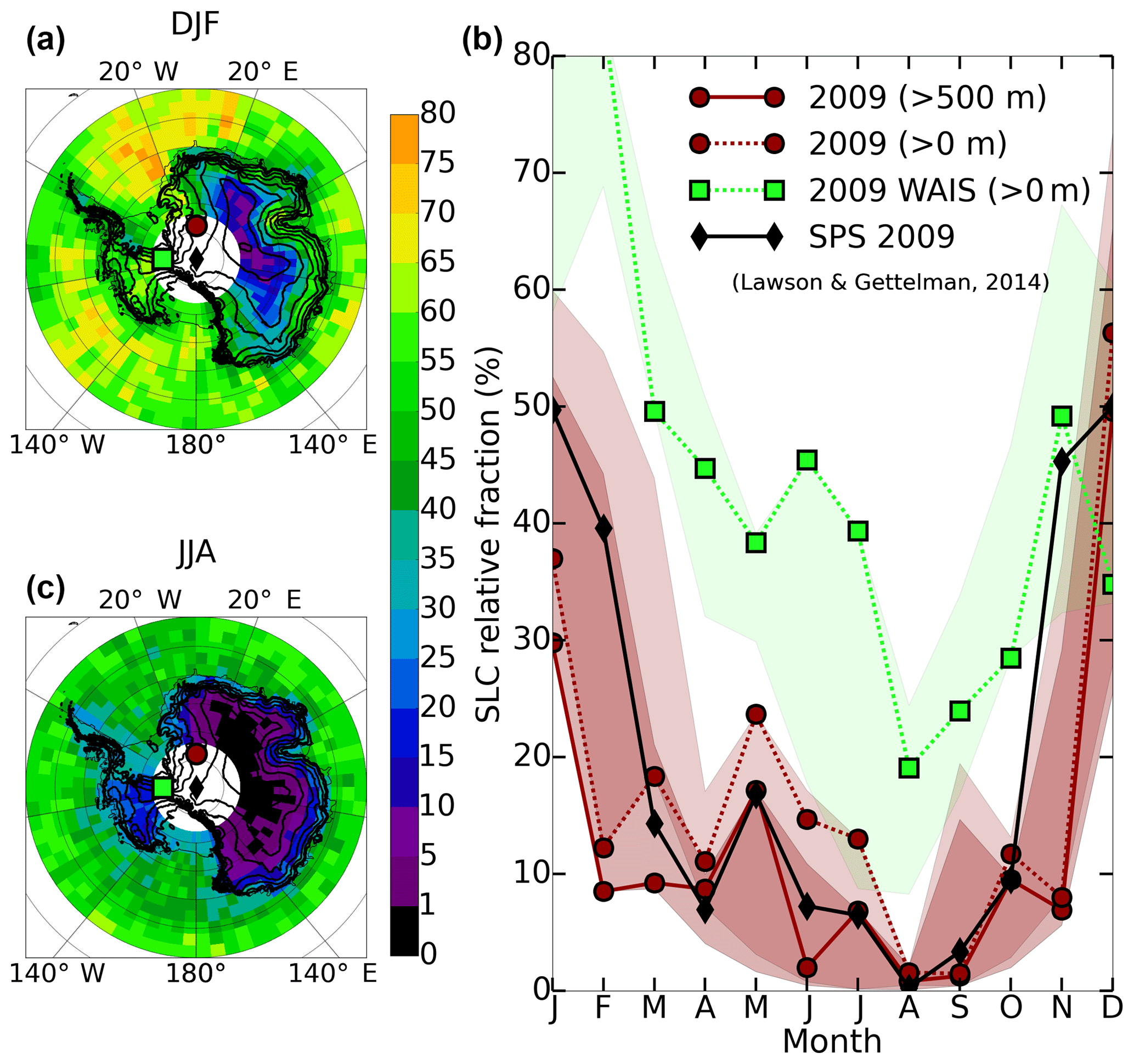
Figure 13(a, c) Geographical distribution of the 2007–2010 average of the SLC relative fraction in DJF (a) and JJA (c). The diamond marker indicates the Amundsen–Scott South Pole Station (SPS). The circle and square markers indicate the approximate locations of the grid boxes – north of the markers – used to extract the time series in area 1 (circle) and area 2 (square), respectively (see text for exact definition of area 1 and 2). (b) column: Monthly time series of the DARDAR SLC relative fraction in 2009 with (solid red line) and without (dotted red line) the lower altitude cut-off of 500 m, extracted north of the circle marker shown in (a) and (c). The dotted green line shows the time series extracted north of the square marker shown in (a) and (c). The shaded areas represent the corresponding interannual variabilities. The black diamond markers show the relative fraction of mixed-phase clouds observed with the MPL at SPS (2850 m a.s.l.) in 2009 (Lawson and Gettelman, 2014, extracted from their Fig. 2d).
It is remarkable how the seasonal cycles from DARDAR observations with or without cut-off in area 1 show a similar pattern to the ground-based observations despite the different locations investigated. This is in spite of the much larger temporal resolution of the MPL, which continuously observes at a single point and can detect features missed by the satellites (similarly to the ceilometers). It is also clear that area 1 is much more representative of SPS than area 2, where SLC relative fractions are far larger than at SPS during all seasons but SON. Expectedly, the SLC relative fractions in area 1 are larger without the altitude cut-off but only between March and July 2009. The 2009 DARDAR fraction is lower than the SPS observations by 10 % and 20 % (absolute difference) in January and February and by 35 % in November. For the rest of the months, the difference is less than 10 %. Importantly, though, the MPL observations lie in the interannual variability range of the DARDAR observations (with or without cut-off) throughout the year (except in November). These results suggest that cloud and SLW observations at the South Pole are representative of lower latitudes on the plateau and on its outskirts. The contribution of SLCs to clouds clearly maximises in summer with average values of 50 % in December and January for the MPL and 40 % for DARDAR (45 % for the 2007–2010 average). The minimum of the SLC relative fraction is in August for both data sets: 1 % for DARDAR (with and without the altitude cut-off) and 0 % at SPS.
Finally, note that in 2009 the occurrences of mixed-phase clouds at the South Pole were all below 5 km a.s.l. (Lawson and Gettelman, 2014). This is also the highest altitude at which we retrieve SLCs, for terrain as high as SPS, in summer (Fig. 7Bc). The temperatures reported by Lawson and Gettelman (2014) in summer are between −28 and −32 ∘C and this is consistent with our values of −33 to −31 ∘C derived for January on the plateau (Fig. 11a). This successful comparison, although made between different locations, validates the ability of DARDAR to capture the seasonal cycle of the SLC fraction, and more particularly in the southernmost regions probed by the satellites.
4.5 Sea ice, supercooled liquid-water and mixed-phase clouds
The monthly evolution of the various cloud types derived in Sect. 4.3 showed distinct patterns. Here, we investigate the potential links between the low-level clouds and the sea ice. Very recently, two studies investigated the impact of the sea ice on the winter low-level clouds in the Southern Ocean and the Antarctic seas (Wall et al., 2017), and on the summer and spring low-level clouds (Frey et al., 2018), and we compare our results to theirs in Sect. 5.2. For the four seasons we distinguish between the low-level cloud fraction and the low-level SLC fraction. We also keep investigating the complementary all-ice fraction to contrast with the observations of SLCs. As we do not have the information from the DARDAR footprint about the presence or absence of sea ice at the sea surface we use monthly products of the sea ice fraction provided by NSIDC at a resolution of 25 km × 25 km, which we project on the grid we use to map the cloud occurrences (Fig. 2i–l). Hence, we work with the distribution of the sea ice (spatial) fraction derived on a monthly timescale. In each grid box we investigate how often a given type of cloud layer forms on a monthly average basis given the monthly average sea ice fraction in that grid box. In Fig. 14 we show the low-level cloud, SLC and all-ice fractions as a function of the sea ice fraction. We also give the Spearman's rank correlation coefficient computed for each seasonal sample (over the 4 years). We also report the amplitude of change in the different fractions between areas where sea ice fraction is <5 % and areas where the sea ice fraction is ≥95 %. In the following we will refer to this quantity when speaking of the difference in the average low-level fractions between open water and sea ice. All the changes in low-level fractions between open water and sea ice reported here were found to be statistically significant at the 99 % level (using a t test).
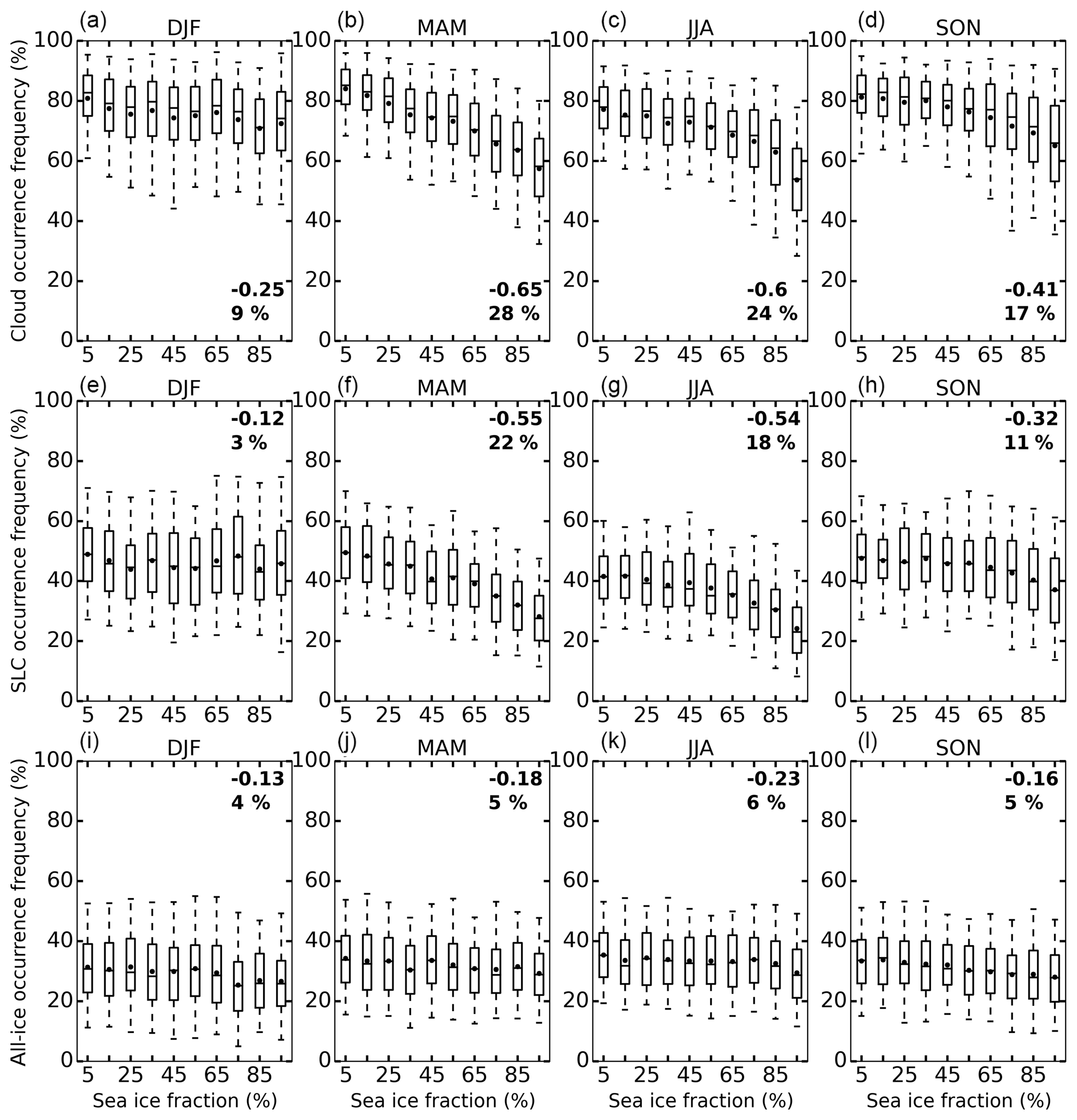
Figure 14Whisker plots with the median (horizontal lines), the mean (circles), the first and third quartiles and the 5 and the 95 percentiles showing – as a function of the sea ice fraction – the evolution of the low-level cloud fraction (a–d), the low-level SLC fraction (e–h) and the low-level all-ice fraction (i–l). The sea ice bin width is 10 %, and the centre value of each bin is labelled on the x axis. Each column represents one season. The Spearman's rank correlation coefficient between the low-level cloud fraction and the sea ice fraction is derived over the whole sample that is used to then compute the whisker plots, and it is indicated at the top-right corner of each panel. The p values for the correlation coefficients are always <0.01. The absolute difference (in %) of occurrence frequency (fraction) of clouds between open water (sea ice fraction <5 %) and sea ice (sea ice fraction >95 %) is indicated below each correlation coefficient.
A clear signal of decreasing low-level cloud fraction as the sea ice fraction increases is detected in autumn, winter and spring (Fig. 14b, c and d), while it is much lower in summer (Fig. 14a), when the negative correlation is the weakest (−0.25) and the absolute change in cloud fraction between open water and sea ice the smallest (9 %). The largest anticorrelation occurs in autumn (−0.6) along with the largest difference in cloud fraction between open water and sea ice (28 %). Note that an equivalent signal is not found for the mid- and high-level cloud fractions (not shown). Comparing the seasonal plots for the SLC fraction (Fig. 14e–h) and for the all-ice fraction (Fig. 14i–l), we conclude that the anticorrelation found between low-level cloud fractions and sea ice fraction is largely due to the SLC fraction changes, rather than to the all-ice fraction changes. The latter show the weakest anticorrelation with sea ice fraction changes (−0.23 to −0.13) with a constant change in amplitude between open water and sea ice (∼5 %) throughout the year. In contrast, the SLC fraction shows the most pronounced anticorrelation with sea ice fraction (−0.55) and the strongest absolute decrease of its value (22 %) in autumn. In winter these values are −0.54 and 18 %, while in spring they are −0.32 and 11 %. In summer, the SLC fraction shows the weakest correlation coefficient of all coefficients derived here (−0.12) and the smallest seasonal change between open water and sea ice (3 %). The contrasting behaviour between SLC fractions and all-ice fractions demonstrates that the latter are not driven by sea ice variability, at least to the point of inducing clear changes in their values when sea ice fraction varies.
In Fig. 15 we further distinguish between low-level MPCs and USLCs since distinct monthly time series prevailed for both cloud types (Fig. 9d and e). The strongest anticorrelations with sea ice fraction occurs for the low-level MPC, which also shows the largest change in fraction between open water and sea ice. The strongest anticorrelations for the MPC fractions are observed in autumn and winter with correlation coefficients of −0.54 and −0.51 and changes in fraction of 14 % and 11 % between open water and sea ice. The difference between open water and sea ice and the anticorrelation with sea ice for the USLC fraction are about two times lower than for the MPC fraction. In spring the anticorrelation weakens and so does the fraction change between open water and sea ice, especially for the USLCs (1 % change against 9 % for MPC). The summer months display strikingly different patterns. The USLC fractions are larger by 5 %–10 % than the MPC fractions, with the largest differences at larger sea ice fractions. The USLC fraction remains within 2 % and no correlation with sea ice fraction is detected (0.03). However, the MPC fractions remains weakly correlated to the sea ice fraction (−0.22) with a 6 % change in fraction between open water and sea ice. With respect to the anticorrelations between MPC or USLC fractions and sea ice fraction the spring months appear between autumn–winter and summer. The MPCs always display some anticorrelation with sea ice fraction, while the USLCs are not correlated with the sea ice fraction in summer and are less than MPC fractions in other seasons. These observations suggest a stronger link between MPCs and sea ice than between USLCs and sea ice. More generally they show that the low-level cloud fraction variability as a function of sea ice is more driven by one of the low-level MPCs. This strongly points to a link between glaciation processes in clouds and sea ice variability.
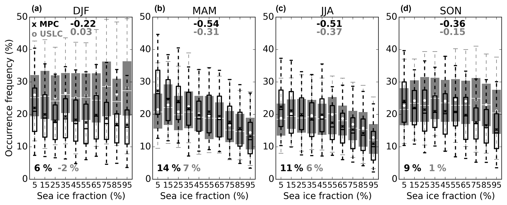
Figure 15Same as Fig. 14 for the low-level MPC (narrow empty black boxes, with a cross showing the average) and USLC (larger shaded grey boxes, with a white circle for the average) fractions. The p values for the correlation coefficients are always <0.01, except for the USLC fraction in summer (p value =0.06).
In order to illustrate the way sea ice spatial variability affects the lower atmosphere, we derive the differences in potential temperature between the surface pressure level (θSLP) and the 850 hPa pressure level (θ850 hPa) at all seasons, for all years. We use the ECMWF temperature and pressure profiles collocated with the satellite overpasses at the DARDAR footprint level and provided with the DARDAR products. The difference θ850 hPa-θSLP is an indicator of the coupling between the sea surface and the atmosphere (e.g. Klein and Hartmann, 1993; Kay and Gettelman, 2009). The pressure level 850 hPa roughly corresponds to a representative altitude level where we find low-level MPC. A larger difference in potential temperature indicates a stronger surface static stability and a weaker coupling between the sea surface and the atmosphere. In this case, the exchange of heat and moisture between the sea surface and the atmosphere is not favoured. The potential temperature difference is plotted as a function of sea ice fractions in Fig. 16. We derive the Spearman's rank correlation coefficient between the potential temperature difference and the sea ice fraction, as well as the difference in θ850 hPa-θSLP (near-surface atmospheric stability) between open water and sea ice. The largest near-surface static stability variations between open water and sea ice are found in autumn and winter (9 and 8 K, Fig. 16b and c), and intermediate stability variation is found in spring (5 K amplitude, Fig. 16d), while no dependency of the sea-surface–atmosphere coupling on sea ice fraction is observed in summer (Fig. 16a). This is in agreement with the differences observed for the low-level SLC, MPC and USLC fractions between open water and sea ice. This difference decreases in autumn, winter, spring and summer, in that order. The same observation can be made for the strength of the anticorrelation with the sea ice fraction, which is the largest for both the near-surface stability and the SLC (MPC) fraction in autumn, winter, spring and summer, in that order. These results support the idea that the decrease in the SLC fraction (which comes mainly from the MPC fraction) with the sea ice fraction increase is caused by a reduction in the coupling between the sea surface and the atmosphere. It is interesting to note that in summer, however, while the strength of the coupling between the sea surface and the atmosphere does not vary as a function of the sea ice fraction, the MPC fraction still shows some variation. This will be discussed below.
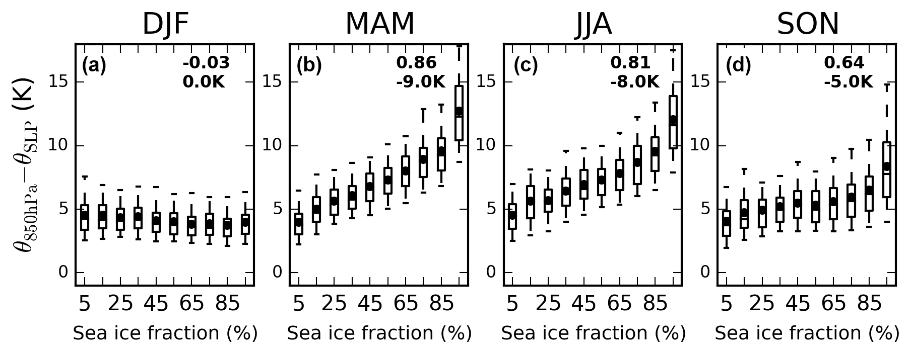
Figure 16Whisker plots showing the potential temperature difference θ850 hPa-θSLP as a function of the sea ice fraction for each season. The potential temperatures are derived from the ECMWF temperatures and pressure profiles are collocated with the satellite overpasses at the DARDAR footprint level. The Spearman's rank correlation coefficient between θ850 hPa-θSLP and the sea ice fraction is derived over the whole sample that is used to then compute the whisker plots, and it is indicated at the top-right corner of each panel. The p values for the correlation coefficients are always <0.01, except for summer (p value =0.03). The absolute difference (in K) in near-surface static stability between open water (sea ice fraction <5 %) and sea ice (sea ice fraction >95 %) is indicated below each correlation coefficient.
5.1 On the clear differences between supercooled-liquid-containing clouds and all-ice clouds
The average total cloud fraction in the Antarctic region is around 68 % at any time of the year, each year (Fig. 9a), demonstrating the absence of Antarctic-wide seasonal or interannual variability. However the Antarctic-wide SLC fraction decreases from ∼47 % in summer to ∼23 % in winter (Fig. 9b). The complementary all-ice fraction increases accordingly. The largest seasonal variability for the total cloud fraction is found on the plateau as noted by previous studies (Verlinden et al., 2011; Adhikari et al., 2012), and it is exclusively due to the all-ice fraction given the same values of cloud and all-ice fractions over the plateau (Fig. 9a and c). The lowest seasonal cloud fractions are found in the eastern part of the plateau in the so-called megadune region (120–160∘ E; 75–82∘ S) in summer (Fig. 5). This minimum in the cloud and all-ice fractions is not detected in the SLC fraction which has a more zonally homogenous distribution in EA (Fig. 5e–h). The megadune region actually witnesses the lowest occurrence of clouds all year. The weak anticyclonic continental circulation creates a centre of higher pressure (Fig. 2a) associated with the strongest subsidence of air in that region (Verlinden et al., 2011). Consistently, it also corresponds to an area where the lowest snowfall rates were mapped by Palerme et al. (2014) and more particularly to the areas with the lowest contribution of snow to the overall accumulation (see their Fig. 6). Interestingly, it is also the area with the most blowing snow events reported from CALIPSO observations (Palm et al., 2017). This could be partly explained by the higher ability to detect those blowing snow events in an area of minimum cloud fraction.
Additionally, we do not expect blowing snow to bias our all-ice fraction. Using a dedicated algorithm based on CALIOP signal, Palm et al. (2017) showed that the blowing snow layer depth in Antarctica was on average 120 m and almost always smaller than 500 m with a depth reaching 1000 m (Palm et al., 2011) on very rare occasions. DARDAR products are not tuned to detect blowing snow and Palm et al. (2011, 2017) demonstrate the need for a specific algorithm for this purpose. However, and interestingly, Lachlan-Cope et al. (2001) mentioned the possible effect of blowing snow on clouds over the Avery Plateau (Antarctic Peninsula) but only for cloud layers in contact with the surface. Lloyd et al. (2015) documented the effect of blowing snow by increasing the number of cloud ice particles in situations of cloud-enveloped surfaces during strong wind events at an alpine site, and Geerts et al. (2015) demonstrated the contribution of turbulent surface-induced processes in the boundary layer over complex terrain, which is certainly relevant to the Antarctic coastal areas. In any case blowing snow is expected to not affect our statistics because of our 500 m lower altitude cut-off and given the little difference between our low-level all-ice cloud statistics by removing the lower altitude cut-off (Fig. B1c). Hence, it is very likely that blowing snow does not bias our low-level cloud fraction statistics even in the (unlikely) case of blowing snow being detected as cloud ice by DARDAR.
The choice of a lower altitude cut-off at 500 m above the surface does not bias our results and discussions as shown in Appendix B. It has the smallest impact on the all-ice fractions (Fig. B1c) and the seasonality of the different cloud types is not altered. Suppressing this cut-off mainly changes the low-level USLC fractions (Fig. B1e), because they can be detected by the lidar down to the surface. However, since it is in the radar blind zone, it is not possible to say whether these USLCs are actually not MPCs. But suppressing the cut-off does not change the shape of the MPC monthly evolution in places where the radar can still assess the presence of ice (Fig. B1d). The ground clutter quickly reduces the number of available observations between 500 m and the surface, but it is not zero (Fig. A1a).
The changes in the SLCs and all-ice fractions do not occur at similar altitudes and are not driven by similar mechanisms. The monthly variability in all-ice fractions increases with altitude over marine regions (from 5 % at low levels up to 30 % at high levels, Fig. 10d–f). The all-ice fraction maximises in winter and autumn as a consequence of the increase in storm activity and deep clouds (Adhikari et al., 2012). Over the continent the changes in all-ice fractions are large already at low-altitude levels, because of the interactions of air masses with the orography and especially where the permanent low-pressure systems around the continent are (Fig. 6a–d). In these places the vertical extension of the cloud (or equivalently, all-ice) fraction is also the largest, especially in winter (e.g. Fig. 7Ah an di) with the strengthening of the lows and the increased cyclonic activity near the coasts (Simmonds et al., 2003). The overall amplitude of change of the low-level all-ice fraction is larger on the WAIS (∼20 %) than on the plateau (15 %). This can be explained by the location of the WAIS closer to the sea and to the ASL. At mid-levels and high-levels the continental all-ice fractions increase by 30 %–35 % in winter as a consequence of synoptic-scale systems made of deep clouds reaching the interior. The SLC fraction decreases poleward, reaching <1 % at 82∘ S in EA compared to 35 % in WA. This difference is due to the increasing surface height polewards, which reaches higher altitudes in EA where the plateau lies, with the coldest temperatures year long.
5.2 On the links with sea ice
In contrast to the all-ice fraction, the seasonality of the SLC fraction is largely driven by its low-level part. It is determined by the tropospheric temperature and sea ice fraction seasonality. This result is in line with the observations made over the Ross Sea and Ross Ice Shelf by Jolly et al. (2018), that the occurrences of liquid-containing clouds varied more as a function of seasons than of circulation regimes in that region. Our results suggest it is actually the case Antarctic-wide. The anticorrelation of the low-level cloud fraction with sea ice fraction is clearly due to the SLC fraction and not to the all-ice fraction (Fig. 14). This points to an exclusive link between liquid-containing cloud formation and sea ice fraction evolution. The largest anticorrelations between the low-level SLC fraction and the sea ice fraction occurs in autumn and winter (Fig. 14f and g) when the sea-surface–atmosphere coupling strength also shows the strongest anticorrelation with sea ice fraction (Fig. 16b an c). No correlation occurs in summer (Fig. 14e), when no variation in sea-surface–atmosphere coupling with the sea ice fraction is observed (Fig. 16a). The spring case (Fig. 14h) is between winter–autumn and summer. The sea ice extent is at its lowest in summer so, at this time of year, more sea ice points will be close to the ice edge than in other seasons and the vertical (potential) temperature gradient will be the smallest. Hence, in summer, advection of cloud may be a more important control on cloudiness at a given location than local processes controlled by sea ice concentration. The lack of correlation between the SLC fraction and the sea ice fraction in summer (Fig. 14e) is consistent with the lack of cloud cover differences between open water and sea ice found by Frey et al. (2018) in the Southern Ocean, and with the similar findings in the Arctic (Kay and Gettelman, 2009; Taylor et al., 2015; Morrison et al., 2018).
The reduction in our winter SLC fraction between open water and sea ice (18 %) is strikingly similar to the reported value by Wall et al. (2017) (17 % between areas with sea ice fraction of 95 % and areas of a sea ice fraction of 0 %). Wall et al. (2017) investigated the effect of advection of cold air off of the sea ice edge (low-level jets), which caused clouds to form right above the nearby open waters in the Southern Ocean. This agreement occurs despite the fact that they work in the 2006–2014 period, while we investigate the 2007–2010 period. Also, we use a combined radar–lidar product, while they use a lidar-only product (GCM-oriented CALIPSO Cloud products developed by Chepfer et al., 2010). However, it is the SLC part of the cloud fraction, which anticorrelates with sea ice fraction, and SLCs are detected with the lidar. Our low-level cloud fractions are 78 % and 54 % over open water and sea-ice. Cloud fractions by Wall et al. (2017) are ∼70 % and ∼50 % (their Fig. 9a). Our larger values of cloud fraction can be explained by our additional use of the radar while Wall et al. (2017) will miss more low-level clouds due to lidar signal extinctions. Nonetheless the cloud fractions are in agreement by <10 %.
In spring, the 11 % difference in the SLC fraction between open water and sea ice is larger than the one reported by Frey et al. (2018) over the SO (4 %). This difference is even larger (17 %) when considering our low-level cloud fraction, mainly because of a slight difference (5 %), also seen in the all-ice clouds. Our low-level cloud fraction in spring is 81 % over open water and 64 % over sea ice. Their low-level cloud fraction is 68 % over open water and 64 % over sea ice. While our respective low-level cloud fractions are the same over sea ice (64 %), they are strikingly different over open water (81 % vs. 68 %). Deeper clouds will form over open water than over sea ice (Wall et al., 2017; Frey et al., 2018; Morrison et al., 2018), and this may explain the difference between our radar–lidar cloud detections and their lidar-only detections over open water. It is unclear, though, what else could contribute to this difference over open water. In summer, a similar difference occurs between our value (81 %) and their value (68 %) over both open water and sea ice. In summer, the occurrences of lidar attenuation are actually larger than in spring and particularly between 2000 m and 3000 m a.s.l. (Frey et al., 2018, their Fig. 8). It is beyond the scope of the paper to further compare lidar-only and radar–lidar products. However, this should be addressed in future studies.
Breaking the SLC fraction down to its MPC and USLC components, we showed a stronger anticorrelation with sea ice fraction for the MPC fraction than for the USLC fraction (Fig. 15). Interestingly, in summer the USLC fraction shows no anticorrelation with sea ice fraction, while the MPC fraction does to some extent (Fig. 15a). It is in spring and summer that both fractions differ the most in both their values and anticorrelation strength with sea ice (Fig. 15a and d). This can be related to the different monthly variability of the MPC and USLC fractions (Fig. 10g and j). In order to discuss these differences in more detail we plot the monthly time series for each marine region separately (Fig. 17). We also add all of the Antarctic seas and the ocean (Fig. 17a) and – as an element of comparison – the Antarctic continent for surface height above 1.5–3 km a.s.l., i.e. away from the coasts (Fig. 17f). The monthly time series of the sea ice fraction is also represented and its y axis is flipped to help with the interpretation.
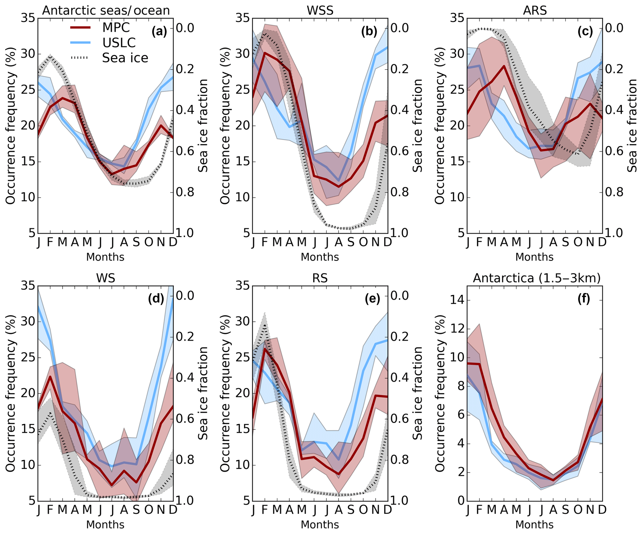
Figure 17Four-year (2007–2010) average monthly time series of the low-level MPC fraction (black line) and the low-level USLC fraction (blue line), for the whole Antarctic waters (a) and for Antarctica (f) for surface heights between 1.5 km and 3 km a.s.l., as well as for the marine regions defined in Fig. 4b–eİn each plot, the monthly time series of the sea ice fraction (dotted line, labelled on the right y axis that is flipped) is also plotted when relevant. The shaded areas indicate the amplitude of variation between the maximum and the minimum monthly averaged fractions recorded over 2007–2010.
Looking at the differences between monthly time series of MPC fractions and USLC fractions as well as the time series of the sea ice fraction, it can be understood why the MPC fractions weakly anticorrelate with the sea ice fraction in summer, while the USLC fractions do not at all in Fig. 15a. This is related to the maximum of the MPC fraction by February or March, which is concomitant of the minimum in sea ice fraction (Fig. 17a–d). In contrast, the USLC fraction decreases from January onwards. This difference between MPCs and USLCs is observed for all the Antarctic seas taken together (Fig. 17a). On the continent, however, both seasonal cycles of the MPC and USLC fractions have the same pattern (Fig. 17f). The further away from the coast it is, the more marked the maximum of the MPC fraction is by the end of summer and beginning of autumn (compare ARS and WSS with WS and RS). WSS and ARS are areas where the clear increase in the sea ice fraction starts later (March–April) than in WS and RS (February). Also, the monthly evolution of the MPC fractions has a larger amplitude for larger monthly sea ice variations (compare WSS and ARS in Fig. 17b and c) as well as – consistently – a larger amplitude in the surface static stability monthly variation (not shown). In autumn, the MPC fraction decreases more strongly in WSS than it does in ARS, and its values in WSS are below that of ARS by the end of that season. In winter, the MPC fraction in WSS is smaller by 5 %–10 % than in ARS (Fig. 10g). In parallel, the sea ice fraction increases from 0.05 to 0.95 in WSS, but only from 0 to 0.6 in ARS. Overall, these observations point to a possible role of the sea ice in modulating the seasonality of the glaciation processes leading to MPC. The “surplus” of anticorrelation with sea ice found for the MPC fraction compared to the USLC fraction (Fig. 15a) hints towards an additional factor in the link between sea ice and the formation of a mixed phase. This would come on top of the role of sea ice melting in the strengthening of sea-surface–atmosphere coupling (Fig. 16) and the release of moisture that drives the formation of SLCs as a whole.
The near-surface conditions (atmospheric temperature and water vapour mass mixing ratio) are similar below MPCs and USLCs over seas (Fig. 11c and d). Consistently, the near-surface static stability below either MPCs or USLCs is the same (not shown). This suggests that it is not a stronger coupling of the sea surface with the atmosphere at particular places that drives the difference between MPC and USLC seasonalities overall, notably by the adiabatic cooling caused by enhanced upward motions where the coupling is stronger. Hence, differences in surface atmospheric states cannot explain the stronger correlations of the MPC fraction with the sea ice fraction compared to the USLC fraction. The average altitude of MPCs is higher than that of USLCs, and the former are logically associated with colder temperatures than the latter (hence more glaciation process is favoured). However, it is not the temperature seasonal cycle alone that is responsible for the differences between the MPC and the USLC seasonal cycles, since the temperatures measured at the top of both cloud types show a similar and simpler seasonal evolution (Fig. 11a). Importantly, Fig. B1 (used for testing the sensitivity of our results to the choice of the lower altitude cut-off) shows that, above 1000 m a.s.l., where MPCs dominate compared to USLCs (Fig. 8), the seasonal cycle of USLCs still differs from that of MPCs in a similar way to how it does with the 500 m a.s.l. cut-off. Finally, the difference between the MPC and the USLC seasonal cycles cannot be an artefact caused by the radar signal loss since the radar clutter occurrences do not show any seasonality (Fig. A2a).
5.3 On the marine origin of the (biological) INPs
The remaining option is to consider the aerosols, and more particularly, the availability of ice-nucleating particles (INPs). The open ocean is a documented source of INPs via sea spray emissions (Burrows et al., 2013; Wilson et al., 2015; DeMott et al., 2015). INPs are most probably of organic origin (e.g. phytoplankton exudates, according to studies performed in the Arctic seas; Wilson et al., 2015), and their emission is possibly favoured by blooming events (from laboratory experiment; DeMott et al., 2015). The marine MPC layers form at an average temperature range of −15 to −5 ∘C (Fig. 8A). At these temperatures samples of collected particles were found to be active INPs in the immersion freezing mode (Wilson et al., 2015; DeMott et al., 2015).
The number concentration of Antarctic aerosols – of which the INPs will be a subset – has been shown to have a seasonal cycle that is well documented. For instance, Weller et al. (2011) and Kim et al. (2017) documented the monthly variation in the total aerosol concentration at the coast in the Weddell Sea sector (Neumayer Station) and at the northern tip of the Antarctic Peninsula (King Sejong Station), respectively. They found that the maximum concentrations occurred in February (Kim et al., 2017, their Fig. 6) or March (Weller et al., 2011, their Fig. 3). Moreover, the increase in aerosols at the end of the year in November–December is much reduced or paused (Weller et al., 2011). Interestingly, in our monthly time series by the end of spring, while the sea ice has already started melting and the USLC fraction is still increasing, the MPC fraction stops increasing in November–December as well (Fig. 17a). In these studies, the authors relate to the enhanced biological activity that prevails with increased solar radiations and sea ice retreat at the sea surface, where phytoplankton grow. They further highlight the possible role of new particle formation (NPF) in the variations in the total aerosol number concentration. Enhanced NPF caused by biological emissions could be an indication of enhanced direct emission of primary biological aerosols as well. Hara et al. (2011) measured the aerosol seasonal cycle at different altitudes using a tethered balloon system in Syowa Station (coastal EA). They demonstrated similar seasonal cycles to those found by Kim et al. (2017). Interestingly, above 1 km a.s.l. – i.e. the typical altitudes at which we detected MPCs – the absolute maximum in aerosol concentration occurred at the beginning of February with a local maximum at the start of November (at least in the range 1 km–1.5 km a.s.l.). Hence, the measured seasonal cycle of the aerosols at the coasts shows striking similarities with that of our MPC fractions. Hara et al. (2011) trace back the highest concentrations with air masses coming from above the SO, emphasising the role of biological activity as an emitter of aerosols or aerosol precursors, of which INPs should happen to be a subset. In fact, the melting of sea ice initiates phytoplankton blooms and the primary production of phytoplankton happens to maximise in January on average (Petrou et al., 2016), and open water reaches its maximum area at the start of February. On smaller scales, though, the production of phytoplankton may appear much more complex, with different local seasonal cycles in a given region (Park et al., 2010). However, and overall the aerosol monthly variability observed at Antarctic coastal stations and related to the biological activity at the sea surface, matches the one of the MPC fraction. Previous studies demonstrated a link between the number of cloud droplets and chlorophyll a concentration (a proxy for phytoplankton biomass) at the sea surface (McCoy et al., 2015). But this is the first time that an indirect signature of the role of biological activity – or say marine aerosols – in glaciation process is pointed at in the observed monthly evolution of mixed-phase cloud occurrences. The time lag between the month of the maximum primary production (January, on average) and the month with the largest MPC fractions (February, on average) could be related to the life cycle of phytoplankton blooms, the demise of which eventually triggers the release of organic material (e.g. exudates) in about 3 weeks to a month (O'Dowd et al., 2015). This would then come along with the surface area of emission of biological INP via sea spray (i.e. open water) being the largest in February.
Interestingly, the Weddell Sea sector is the area with the highest SLC fractions in summer (Fig. 5e) in all years but 2009, when parts of the Amundsen–Ross sector (Fig. 4c) have equally large values (it is also the area with the largest relative contribution of SLCs to low-level clouds as shown by Fig. 13a). This regional increase in SLC fractions in summer is mainly due to an increase in the MPC fraction (Fig. 10g) rather than in the USLC fraction (Fig. 10j). Interestingly, the Weddell Sea sector sits in a part of the SO where chlorophyll a concentration reaches the highest values and has the largest average values throughout the year compared to anywhere else around the continent (Blondeau-Patissier et al., 2014). This observation is in line with our hypothesis of the marine MPC fraction monthly evolution being modulated by the bioaerosol seasonal emissions.
The Weddell Sea shows up as a particularly favourable area for SLW formation in summer (Fig. 7Bb). More particularly, the eastern part of it shows up as a hotspot for maintaining USLC layers in that season (Figs. 6i and 8Bb) up to 1 km a.s.l. No other coastal area shows a similar pattern. This is consistent with recent aircraft measurements during the Microphysics of Antarctic Clouds (MAC) campaign in summer 2015 in the eastern Weddell Sea, where persistent supercooled liquid layers were observed at around 1 km altitude, with only rare and very localised occurrences of patches of ice (O'Shea et al., 2017). A plausible explanation for this is the dominant easterly circulation there, which brings more air masses with more continental influences, hence decreasing the effect of marine INPs. The liquid-dominated layer clouds probed during MAC had a cloud top almost systematically in the range 500–1500 m a.s.l., and their in-cloud temperature was between −5 and −15 ∘C (except from one frontal cloud) (O'Shea et al., 2017, their Table 1). This is consistent with the altitude ranges and temperatures reported for the SLC fractions (Fig. 8). Comparisons between the MAC aircraft measurements and summer satellite observations will be carried out in a separate study. Importantly, (O'Shea et al., 2017) demonstrated the importance of secondary ice production in the formation of the localised patches of ice in the eastern Weddell Sea and this mechanism was also evidenced in the Antarctic Peninsula region by Grosvenor et al. (2012); Lachlan-Cope et al. (2016). Given the relatively warm temperatures at which this ice multiplication process occurs (Hallett–Mossop process between −3 and −8 ∘C; Hallett and Mossop, 1974), we can expect it to happen mainly in the lowest clouds, where the radar may not be always able to detect the presence of ice (thereby distinguishing between USLCs and MPCs). In the Weddell Sea, the SLCs are mainly USLCs at temperatures larger than −10 ∘C and altitudes higher than 500 m a.s.l. (Figs. 7Bb and 8Bb) and the rare patches of ice (O'Shea et al., 2017) may be too small for the radar footprint to resolve them.
It is possible that USLCs or MPCs are more prevalent than suggested by our study at low altitudes since the detection of an SLC at – say – 1000 m a.s.l. will prevent the detection of another SLC below. In this respect, year-long ground-based measurements of microphysical properties of the mixed phase and the primary ice production appear as a needed complement. Note that O'Shea et al. (2017) found no clear trend of an increased number of ice crystals with air masses originated from the SO. This is contrary to our hypothesis of marine INPs driving the glaciation process. However, the limited number of localised patches of ice probed by the aircraft in a restricted period of time, in an area relatively more influenced by continental air masses, might have rendered this task difficult. Note that another area with higher USLC than MPC occurrences was the interior of the WAIS (Fig. 8Bc), an environment relatively more influenced by continental air masses devoid of marine INPs. Our results suggest that satellite observations and their large statistics may indirectly help answer the question of the origin of primary ice production – the first ice – in Antarctic clouds.
Finally, biological activity can also create cloud condensation nuclei (CCN). Why do not we then observe a similar pattern in the USLC seasonal cycle? Recall that we observe larger regional relative differences between the MPC fractions than between the USLC fractions (Fig. 9d and e). This suggests a regional dependence on INP availability and much less on CCN availability. While CCN emission can at least partly be the result of biological activity (McCoy et al., 2015) as initially put by the well-known CLAW hypothesis (Charlson et al., 1987), they are also provided by sea salt emission via bubble-bursting (Quinn and Bates, 2011) or blowing snow from over the sea ice (Yang et al., 2008; Legrand et al., 2016). Hence, the availability of CCN is probably much less dependent on biological activity (Quinn and Bates, 2011). Sea salt is not an INP at (warm) temperatures (Burrows et al., 2013) at which we detect MPCs (T≥15 ∘C). Another open question remains regarding the aerosol seasonal cycle over the plateau (Fiebig et al., 2014, and references therein) and its outskirts, where it is argued that the aerosol baseline originates from the free troposphere and the lower stratosphere in the descent of air happening at these locations (Fiebig et al., 2014) and how these aerosols may or may not affect cloud formation and/or glaciation processes in the continental clouds.
We demonstrated the geographical, vertical and seasonal distribution of the occurrence frequency (fraction) of supercooled liquid-water-containing clouds (SLCs) in the Antarctic region (60–82∘ S) using the radar–lidar DARDAR-MASK v2 products. We described it in comparison to the total cloud fraction, and notably to clouds involving only ice microphysics (all-ice). The combination of the radar and the lidar signals allowed us to further distinguish between mixed-phase clouds (MPCs) and unglaciated (pure) supercooled liquid-water clouds (USLCs) at the pixel level. The Antarctic-wide average total cloud fraction – derived with DARDAR for altitudes above 500 m above the surface – is around ∼70 % and has little interannual variability (≤5 % absolute variation). The Antarctic-wide total SLC fraction varies from ∼50 % in summer to ∼20 % in winter, while the opposite is found for the all-ice fraction. The Antarctic-wide total MPC and USLC fractions have distinct seasonal cycles. While the USLC fraction is maximum in December–January (∼20 %) and minimum in August (∼10 %), the MPC fraction maximises at the end of summer (February, ∼30 %) or in autumn, and it is at minimum in July–August (∼10 %).
The total cloud fraction has the largest monthly variability on the plateau, while its evolution on the WAIS shows an almost constant fraction from February to October (65 %–70 %). However the continental all-ice fraction maximises in winter and is larger on the WAIS (60 %) than on the plateau (50 %), and the monthly variability is larger over the WAIS (+40 % absolute difference from summer to winter) than over the plateau (+30 %). This results from the WAIS being in closer contact to the ASL, which leads to orographic (all-ice) cloud formation. The geographical and vertical distribution of the all-ice fraction is shaped by the orography and its interactions with the permanent low-pressure systems, which are located around the continent, more particularly on the WAIS and south of the AIS. This is particularly evident in winter. In all marine and continental regions the all-ice fraction maximises in winter, when cyclonic activity increases and storms are more numerous over seas. On the continent the cloud fraction monthly variability at mid- and high-level is the largest of the whole Antarctic region and it is exclusively driven by all-ice clouds. Over the Antarctic seas and the SO, the total cloud fraction monthly variability is driven by the low-level SLC fraction variability. Conversely, the mid- and high-level cloud fractions are driven by the mid- and high-level all-ice fractions.
The geographical distribution and seasonality of the SLC fraction is shaped by the temperature seasonal cycle and the sea ice fraction seasonal evolution, which drive the amount of water vapour released into the atmosphere. On the continent the SLC fraction decreases polewards as a result of decreasing temperatures. It is at minimum on the plateau, where it reaches almost zero (<1 %) by winter. We validated our observations of SLC fractions close to 82∘ S by comparing them to opportune ground-based measurements made at the South Pole Station in 2009 with a micropulsed lidar. We demonstrated the representativity of the South Pole for lower latitudes on the plateau, in terms of SLC seasonal cycle measurements. On the WAIS, where the largest continental SLC fractions are found, the detected SLCs are mainly in the form of USLCs and not MPCs, which is reminiscent of the characteristics of lenticular mountain wave clouds. In marine regions, MPCs are principally detected between 1 km and 1.5 km a.s.l., while USLCs dominate between 0 and 1 km a.s.l. The temperature range characteristic of marine MPCs is −15 to −5 ∘C.
The low-level SLC fraction is responsible for the anticorrelation of the low-level cloud fraction with the sea ice fraction, while the all-ice fraction does not show a clear dependency on the sea ice variability throughout the year. The strongest anticorrelations of the SLC fraction with sea ice fraction occur in autumn and winter, when the surface static stability (sea-surface–atmosphere coupling) also shows the strongest response to varying sea ice fraction. The low-level SLC fraction decreases by 22 % and 18 % in amplitude from open water to sea ice in autumn and winter, respectively. In summer, little anticorrelation is found between the low-level SLC fraction and the sea ice fraction, in agreement with a lack of correlation between surface stability and sea ice. Our results are in agreement with recent studies investigating links between sea ice in winter, spring and summer and using lidar-only products.
The monthly time series of the low-level MPC fraction shows a distinct maximum by the end of summer or beginning of autumn, which is absent for the low-level USLC fraction, which maximises at the end of December. This difference is observed over marine areas and not over the continent and it is more marked for the Weddell Sea sector and Amundsen–Ross sector than for the Weddell and the Ross seas, which are closer to the coast. Importantly, the monthly variations in the low-level MPC fraction match the documented seasonal cycle of aerosols in coastal Antarctic stations, which is driven by the biological activity in spring and summer when sunlight increases and sea ice melts. To our knowledge, this is the first time that a link is made between the seasonal cycle of aerosols (of which the INPs are a subset) and the seasonal cycle of mixed-phase clouds over the Antarctic waters. Based on the literature, our results point to the signature of INP emissions from biological activity at the sea surface in the monthly evolution of mixed-phase clouds.
Using satellite products, we provided constraints on the Antarctic-wide distribution of supercooled liquid water and its monthly or seasonal evolution. The radar–lidar synergy appears as a promising tool for pinning down some fundamental links between the glaciation process of polar clouds, supercooled liquid water and biological activity at the sea surface, in association with sea ice variability. We plan to extend our investigation with DARDAR products to more recent years as well as to compare them with more recent field campaigns measuring supercooled liquid water. Surface-based and aircraft measurements of cloud microphysical properties and of the nature of the aerosols, on the coast and offshore, would help test our hypothesis of the MPC seasonal evolution being modulated by the release of marine (biological) INPs.
The DARDAR-MASK v2 products are available on the Aeris/ICARE data centre (http://www.icare.univ-lille1.fr/, last access: December 2017).
Contamination of the radar signal by surface echoes and lidar extinctions or attenuations due to optically thick ice clouds or supercooled liquid layers reduce our statistics as we observe closer to the ground. Figure A1 illustrates this for the summer season (when the lidar signal extinctions are the more numerous, because of higher occurrences of SLCs). Transects are derived by averaging the occurrence frequency of each of the signal contamination over the three latitudinal bands presented in Fig. 4d. The lidar is considered “extinguished” when the surface is not detected. Then all the pixels below the last one detected with a signal are flagged accordingly (Ceccaldi et al., 2013). The lidar is considered “attenuated” when the surface is detected but some features detected by the radar are not seen by the lidar, and the corresponding pixels are flagged accordingly (Ceccaldi et al., 2013). The radar signal is contaminated below 1 km above the ground, with a ∼40 % loss of valid observations at 500 m above the surface (Fig. A1a, b and c). In the coastal areas the contamination occurs more often and affects higher altitudes over terrain with steep slopes (Fig. A1b, compare 0–40 and 50–150∘ E). The lidar extinctions or attenuations depend on the season and more (less) loss will occur at high (low) altitudes in winter over the interior of the WAIS (the ocean) because of more (less) numerous thick ice clouds (SLCs).
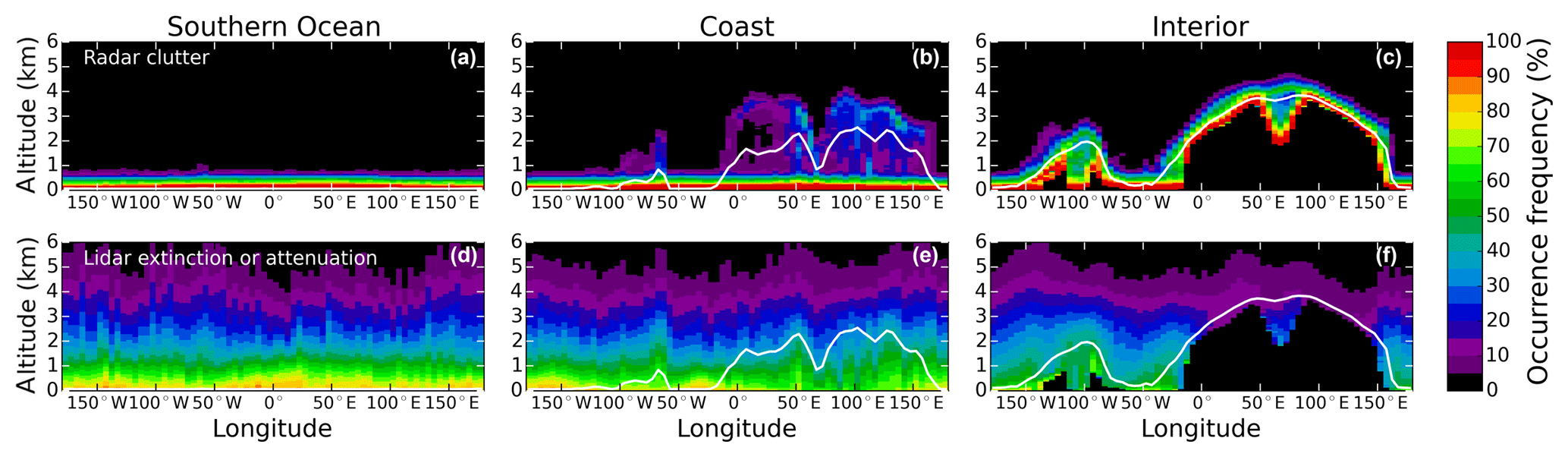
Figure A1Vertical transects (2007–2010 average) showing the occurrence frequency (%) of the radar clutter contamination (a–c) and the lidar signal extinctions or attenuations (d–f). The transects are averaged over the three latitudinal bands presented in Fig. 4d, namely the Southern Ocean (a, d), the coast (b, e) and the interior (c, f). The data are plotted for the summer season.

Figure A2Monthly time series of the low-level occurrences of the radar clutter (a), the lidar extinctions (b) and the lidar attenuations (c) for the areas defined in Fig. 4c and averaged over 2007–2010. The shaded areas correspond to the interannual variability.
The seasonality of the occurrences of signal losses are shown in Fig. A2. The only type of signal obstruction showing a clear seasonality is the lidar extinctions and this is caused by the seasonality of the SLC fractions as discussed in the main text. The radar clutter is responsible for a loss of ∼40 % of the data at ∼500 m above the surface (the occurrences of the clutter are negligible above 1000 m above the surface).
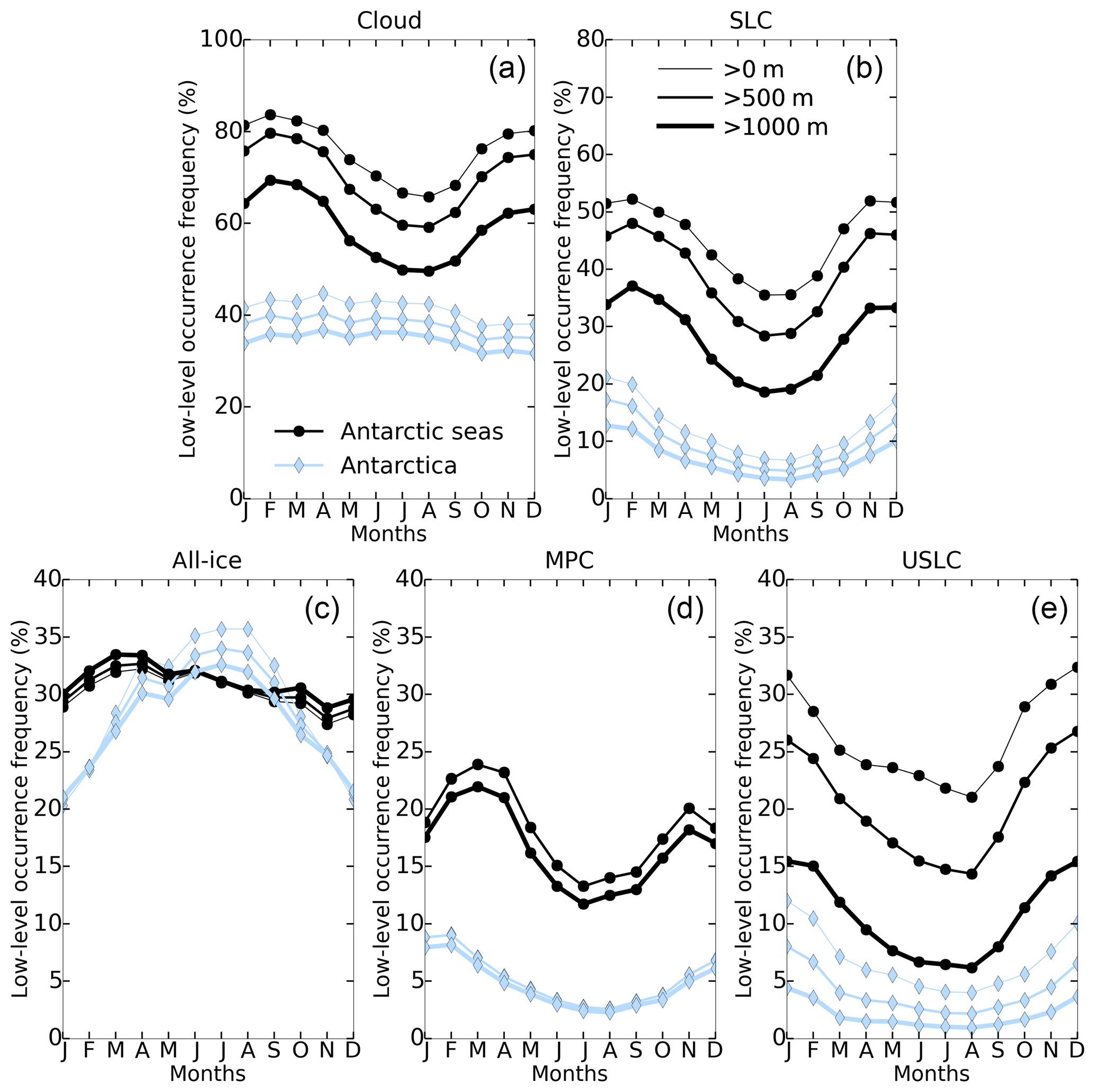
Figure B1Monthly time series of the low-level cloud fraction (a), SLC fraction (b), all-ice fraction (c), MPC fraction (d) and USLC fraction (e) for three different lower-altitude cut-offs: 0 m (thinnest solid line), 500 m (intermediate) and 1000 m (thickest solid line). They are plotted by distinguishing between continental (blue lines) and marine (black lines) clouds. See Sect. 3.2 for the definitions of the phases.
The lower altitude cut-off chosen for deriving the geographical distribution of clouds will affect this distribution at low-levels. This cut-off is used in the present study to avoid low altitudes at which the statistics is significantly reduced because of the radar blind zone and the lidar signal extinctions. A 500 m value was chosen in the present paper. Figure A2 shows the impact of changing this cut-off on the values of the low-level cloud occurrences and on the monthly time series patterns. Changing from a 500 m cut-off to a 1000 m cut-off impacts the SLC fraction (Fig. B1b) and mostly its USLC component (Fig. B1e). There is a 10 % difference between the USLC fraction >500 m (∼20 % yearly average) and the USLC fraction >1000 m (∼10 % yearly average) over seas, where their occurrences are larger than over the continent. Indeed, a large part of the USLCs are detected below 1000 m a.s.l. However the monthly relative variations are not impacted and the seasonal cycle shows similar pattern with the three cut-offs. The difference between the MPC fractions >500 and >1000 m is ∼2 % (Fig. B1d). It is also for the USLC fraction that the difference is the largest between fractions derived without cut-off and with the 500 m cut-off. However, the difference for the MPC fractions is null (Fig. B1d) since these clouds are mainly detected above 500 m above the surface. An additional ∼5 %–8 % of occurrences are added to the USLC fraction when removing the cut-off. The all-ice cloud fractions are only marginally affected in winter over the continent (∼5 % absolute difference between no cut-off and the 1000 m cut-off, Fig. B1c). Overall, changing the cut-off does not change the monthly relative variability of the cloud fraction and the various cloud types fractions, and this only significantly impacts the low-level USLC occurrences over seas. Below 500 m above the surface it is challenging to distinguish between MPCs and USLCs because of the radar blind zone. Hence, all additional SLCs will be identified as USLCs.
CL designed and performed the analysis and wrote the manuscript. JD helped design the study, use the data and write the manuscript. AK derived and analysed the ceilometer cloud fractions and helped write the manuscript. TLC and JK gave advice on the science, the organisation and the writing of the manuscript.
The authors declare that they have no conflict of interest.
We thank two anonymous reviewers, who helped clarify the manuscript and improve the presentation and the discussion of the method through their constructive comments. Constantino Listowski thanks CNES for postdoctoral fellowship funding. Amélie Kirchgaessner, Tom Lachlan-Cope and John King acknowledge the Microphysics of Antarctic Clouds project grant (NE/K01305X/1) funded by the UK Natural Environment Research Council. We thank the Aeris/ICARE data infrastructure for providing access to the DARDAR products used in this study, as well as for the processing of this data and for providing assistance (http://www.icare.univ-lille1.fr/, last access: December 2017). We thank the NASA CloudSat Project and NASA/LaRC/ASDC for making available the CloudSat and CALIPSO products, respectively, which are used to build the synergetic DARDAR products. We thank NOAA and NSIDC for making available the Climate Data Record of sea ice concentration. We thank the mesocentre ESPRI facility for distributing ERAI products in netcdf format, and which is supported by CNRS, UPMC, Labex L-IPSL, CNES and Ecole Polytechnique.
This paper was edited by Michael Pitts and reviewed by two anonymous referees.
Adhikari, L., Wang, Z., and Deng, M.: Seasonal variations of Antarctic clouds observed by CloudSat and CALIPSO satellites, J. Geophys. Res.-Atmos., 117, D00H18, https://doi.org/10.1029/2011jd016719, https://doi.org/10.1029/2011jd016719, 2012. a, b, c, d, e, f
Alexander, S. P. and Protat, A.: Cloud Properties Observed From the Surface and by Satellite at the Northern Edge of the Southern Ocean, J. Geophys. Res.-Atmos., 123, 443–456, https://doi.org/10.1002/2017jd026552, https://doi.org/10.1002/2017jd026552, 2018. a
Baines, P. G. and Fraedrich, K.: Topographic Effects on the Mean Tropospheric Flow Patterns around Antarctica, J. Atmos. Sci., 46, 3401–3415, https://doi.org/10.1175/1520-0469(1989)046<3401:teotmt>2.0.co;2, 1989. a
Blondeau-Patissier, D., Gower, J. F., Dekker, A. G., Phinn, S. R., and Brando, V. E.: A review of ocean color remote sensing methods and statistical techniques for the detection, mapping and analysis of phytoplankton blooms in coastal and open oceans, Prog. Oceanogr., 123, 123–144, https://doi.org/10.1016/j.pocean.2013.12.008, 2014. a
Bodas-Salcedo, A., Williams, K. D., Ringer, M. A., Beau, I., Cole, J. N. S., Dufresne, J.-L., Koshiro, T., Stevens, B., Wang, Z., and Yokohata, T.: Origins of the Solar Radiation Biases over the Southern Ocean in CFMIP2 Models, J. Climate, 27, 41–56, https://doi.org/10.1175/jcli-d-13-00169.1, https://doi.org/10.1175/jcli-d-13-00169.1, 2014. a, b
Bodas-Salcedo, A., Hill, P. G., Furtado, K., Williams, K. D., Field, P. R., Manners, J. C., Hyder, P., and Kato, S.: Large Contribution of Supercooled Liquid Clouds to the Solar Radiation Budget of the Southern Ocean, J. Climate, 29, 4213–4228, https://doi.org/10.1175/jcli-d-15-0564.1, https://doi.org/10.1175/jcli-d-15-0564.1, 2016. a
Bromwich, D. H., Nicolas, J. P., Hines, K. M., Kay, J. E., Key, E. L., Lazzara, M. A., Lubin, D., McFarquhar, G. M., Gorodetskaya, I. V., Grosvenor, D. P., Lachlan-Cope, T., and van Lipzig, N. P. M.: Tropospheric clouds in Antarctica, Rev. Geophys., 50, RG1004, https://doi.org/10.1029/2011RG000363, 2012. a, b, c
Bromwich, D. H., Otieno, F. O., Hines, K. M., Manning, K. W., and Shilo, E.: Comprehensive evaluation of polar weather research and forecasting model performance in the Antarctic, J. Geophys. Res.-Atmos., 118, 274–292, https://doi.org/10.1029/2012jd018139, 2013a. a
Burrows, S. M., Hoose, C., Pöschl, U., and Lawrence, M. G.: Ice nuclei in marine air: biogenic particles or dust?, Atmos. Chem. Phys., 13, 245–267, https://doi.org/10.5194/acp-13-245-2013, 2013. a, b
Cavalieri, D. J., Parkinson, C. L., Gloersen, P., and Zwally, H. J.: updated yearly, Sea Ice Concentrations from Nimbus-7 SMMR and DMSP SSM/I-SSMIS Passive Microwave Data, Version 1. December 2006 to December 2010, 60∘ S to 82∘ S, Boulder, Colorado USA, NASA National Snow and Ice Data Center Distributed Active Archive Center, https://doi.org/10.5067/8GQ8LZQVL0VL, 1996. a
Cazenave, Q., Ceccaldi, M., Delanoë, J., Pelon, J., Groß, S., and Heymsfield, A.: Evolution of DARDAR-CLOUD ice cloud cloud retrieval: new parameters and impacts on the retrieved microphysical properties, Atmos. Meas. Tech. Discuss., https://doi.org/10.5194/amt-2018-397, in review, 2018. a
Ceccaldi, M.: Combinaison de mesures actives et passives pour l'étude des nuages dans le cadre de la préparation à la mission EarthCARE, Climatologie, PhD thesis, Universite de Versailles Saint-Quentin-en-Yvelines, available at: https://hal.archives-ouvertes.fr/tel-01119939 (last access: July 2018), 2014. a
Ceccaldi, M., Delanoë, J., Hogan, R. J., Pounder, N. L., Protat, A., and Pelon, J.: From CloudSat-CALIPSO to EarthCare: Evolution of the DARDAR cloud classification and its comparison to airborne radar-lidar observations, J. Geophys. Res.-Atmos., 118, 7962–7981, https://doi.org/10.1002/jgrd.50579, 2013. a, b, c, d, e, f, g, h, i, j
Charlson, R. J., Lovelock, J. E., Andreae, M. O., and Warren, S. G.: Oceanic phytoplankton, atmospheric sulphur, cloud albedo and climate, Nature, 326, 655–661, https://doi.org/10.1038/326655a0, 1987. a
Chepfer, H., Bony, S., Winker, D., Cesana, G., Dufresne, J. L., Minnis, P., Stubenrauch, C. J., and Zeng, S.: The GCM-Oriented CALIPSO Cloud Product (CALIPSO-GOCCP), J. Geophys. Res., 115, D00H16, https://doi.org/10.1029/2009jd012251, 2010. a
Dee, D. P., Uppala, S. M., Simmons, A. J., Berrisford, P., Poli, P., Kobayashi, S., Andrae, U., Balmaseda, M. A., Balsamo, G., Bauer, P., Bechtold, P., Beljaars, A. C. M., van de Berg, L., Bidlot, J., Bormann, N., Delsol, C., Dragani, R., Fuentes, M., Geer, A. J., Haimberger, L., Healy, S. B., Hersbach, H., Hólm, E. V., Isaksen, L., Kållberg, P., Köhler, M., Matricardi, M., McNally, A. P., Monge-Sanz, B. M., Morcrette, J.-J., Park, B.-K., Peubey, C., de Rosnay, P., Tavolato, C., Thépaut, J.-N., and Vitart, F.: The ERA-Interim reanalysis: configuration and performance of the data assimilation system, Q. J. Roy. Meteor. Soc., 137, 553–597, https://doi.org/10.1002/qj.828, 2011. a
Delanoë, J. and Hogan, R. J.: A variational scheme for retrieving ice cloud properties from combined radar, lidar, and infrared radiometer, J. Geophys. Res., 113, D07204, https://doi.org/10.1029/2007jd009000, https://doi.org/10.1029/2007jd009000, 2008. a
Delanoë, J. and Hogan, R. J.: Combined CloudSat-CALIPSO-MODIS retrievals of the properties of ice clouds, J. Geophys. Res., 115, D00H29, https://doi.org/10.1029/2009jd012346, 2010. a, b
DeMott, P. J., Hill, T. C. J., McCluskey, C. S., Prather, K. A., Collins, D. B., Sullivan, R. C., Ruppel, M. J., Mason, R. H., Irish, V. E., Lee, T., Hwang, C. Y., Rhee, T. S., Snider, J. R., McMeeking, G. R., Dhaniyala, S., Lewis, E. R., Wentzell, J. J. B., Abbatt, J., Lee, C., Sultana, C. M., Ault, A. P., Axson, J. L., Martinez, M. D., Venero, I., Santos-Figueroa, G., Stokes, M. D., Deane, G. B., Mayol-Bracero, O. L., Grassian, V. H., Bertram, T. H., Bertram, A. K., Moffett, B. F., and Franc, G. D.: Sea spray aerosol as a unique source of ice nucleating particles, P. Natl. Acad. Sci. USA, 113, 5797–5803, https://doi.org/10.1073/pnas.1514034112, https://doi.org/10.1073/pnas.1514034112, 2015. a, b, c
Dufour, A., Charrondière, C., and Zolina, O.: Moisture transport in observations and reanalyses as a proxy for snow accumulation in East Antarctica, The Cryosphere, 13, 413–425, https://doi.org/10.5194/tc-13-413-2019, 2019. a
Fiebig, M., Hirdman, D., Lunder, C. R., Ogren, J. A., Solberg, S., Stohl, A., and Thompson, R. L.: Annual cycle of Antarctic baseline aerosol: controlled by photooxidation-limited aerosol formation, Atmos. Chem. Phys., 14, 3083–3093, https://doi.org/10.5194/acp-14-3083-2014, 2014. a, b
Flato, G., Marotzke, J., Abiodun, B., Braconnot, P., Chou, S., Collins, W., Cox, P., Driouech, F., Emori, S., Eyring, V., Forest, C., Gleckler, P., Guilyardi, E., Jakob, C., Kattsov, V., Reason, C., and Rummukainen, M.: Evaluation of Climate Models, in: Climate Change 2013: The Physical Science Basis. Contribution of Working Group I to the Fifth Assessment Report of the Intergovernmental Panel on Climate Change, edited by: Stocker, T. F., Qin, D., Plattner, G.-K., Tignor, M., Allen, S. K., Boschung, J., Nauels, A., Xia, Y., Bex, V., and Midgley, P. M., 2013. a
Fretwell, P., Pritchard, H. D., Vaughan, D. G., Bamber, J. L., Barrand, N. E., Bell, R., Bianchi, C., Bingham, R. G., Blankenship, D. D., Casassa, G., Catania, G., Callens, D., Conway, H., Cook, A. J., Corr, H. F. J., Damaske, D., Damm, V., Ferraccioli, F., Forsberg, R., Fujita, S., Gim, Y., Gogineni, P., Griggs, J. A., Hindmarsh, R. C. A., Holmlund, P., Holt, J. W., Jacobel, R. W., Jenkins, A., Jokat, W., Jordan, T., King, E. C., Kohler, J., Krabill, W., Riger-Kusk, M., Langley, K. A., Leitchenkov, G., Leuschen, C., Luyendyk, B. P., Matsuoka, K., Mouginot, J., Nitsche, F. O., Nogi, Y., Nost, O. A., Popov, S. V., Rignot, E., Rippin, D. M., Rivera, A., Roberts, J., Ross, N., Siegert, M. J., Smith, A. M., Steinhage, D., Studinger, M., Sun, B., Tinto, B. K., Welch, B. C., Wilson, D., Young, D. A., Xiangbin, C., and Zirizzotti, A.: Bedmap2: improved ice bed, surface and thickness datasets for Antarctica, The Cryosphere, 7, 375–393, https://doi.org/10.5194/tc-7-375-2013, 2013. a
Frey, W. R., Morrison, A. L., Kay, J. E., Guzman, R., and Chepfer, H.: The Combined Influence of Observed Southern Ocean Clouds and Sea Ice on Top-of-Atmosphere Albedo, J. Geophys. Res.-Atmos., 123, 4461–4475, https://doi.org/10.1029/2018jd028505, 2018. a, b, c, d, e, f
Frezzotti, M.: Snow megadunes in Antarctica: Sedimentary structure and genesis, J. Geophys. Res., 107, 4344 , https://doi.org/10.1029/2001jd000673, 2002. a
Geerts, B., Pokharel, B., and Kristovich, D. A. R.: Blowing Snow as a Natural Glaciogenic Cloud Seeding Mechanism, Mon. Weather Rev., 143, 5017–5033, https://doi.org/10.1175/mwr-d-15-0241.1, 2015. a
Genthon, C., Berne, A., Grazioli, J., Durán Alarcón, C., Praz, C., and Boudevillain, B.: Precipitation at Dumont d'Urville, Adélie Land, East Antarctica: the APRES3 field campaigns dataset, Earth Syst. Sci. Data, 10, 1605–1612, https://doi.org/10.5194/essd-10-1605-2018, 2018. a
Gorodetskaya, I. V., Kneifel, S., Maahn, M., Van Tricht, K., Thiery, W., Schween, J. H., Mangold, A., Crewell, S., and Van Lipzig, N. P. M.: Cloud and precipitation properties from ground-based remote-sensing instruments in East Antarctica, The Cryosphere, 9, 285–304, https://doi.org/10.5194/tc-9-285-2015, 2015. a, b
Grazioli, J., Genthon, C., Boudevillain, B., Duran-Alarcon, C., Del Guasta, M., Madeleine, J.-B., and Berne, A.: Measurements of precipitation in Dumont d'Urville, Adélie Land, East Antarctica, The Cryosphere, 11, 1797–1811, https://doi.org/10.5194/tc-11-1797-2017, 2017a. a
Grazioli, J., Madeleine, J.-B., Gallée, H., Forbes, R. M., Genthon, C., Krinner, G., and Berne, A.: Katabatic winds diminish precipitation contribution to the Antarctic ice mass balance, P. Natl. Acad. Sci. USA, 114, 1858–10863, https://doi.org/10.1073/pnas.1707633114, 2017b. a
Grosvenor, D. P., Choularton, T. W., Lachlan-Cope, T., Gallagher, M. W., Crosier, J., Bower, K. N., Ladkin, R. S., and Dorsey, J. R.: In-situ aircraft observations of ice concentrations within clouds over the Antarctic Peninsula and Larsen Ice Shelf, Atmos. Chem. Phys., 12, 11275–11294, https://doi.org/10.5194/acp-12-11275-2012, 2012. a, b, c
Hallett, J. and Mossop, S. C.: Production of secondary ice particles during the riming process, Nature, 249, 26–28, https://doi.org/10.1038/249026a0, 1974. a
Hara, K., Osada, K., Nishita-Hara, C., and Yamanouchi, T.: Seasonal variations and vertical features of aerosol particles in the Antarctic troposphere, Atmos. Chem. Phys., 11, 5471–5484, https://doi.org/10.5194/acp-11-5471-2011, 2011. a, b
Haynes, J. M., Jakob, C., Rossow, W. B., Tselioudis, G., and Brown, J.: Major Characteristics of Southern Ocean Cloud Regimes and Their Effects on the Energy Budget, J. Climate, 24, 5061–5080, https://doi.org/10.1175/2011jcli4052.1, 2011. a, b
Heymsfield, A. J. and Miloshevich, L. M.: Homogeneous Ice Nucleation and Supercooled Liquid Water in Orographic Wave Clouds, J. Atmos. Sci., 50, 2335–2353, https://doi.org/10.1175/1520-0469(1993)050<2335:hinasl>2.0.co;2, 1993. a
Hu, Y., Rodier, S., man Xu, K., Sun, W., Huang, J., Lin, B., Zhai, P., and Josset, D.: Occurrence, liquid water content, and fraction of supercooled water clouds from combined CALIOP/IIR/MODIS measurements, J. Geophys. Res., 115, D00H34, https://doi.org/10.1029/2009jd012384, 2010. a
Huang, Y., Siems, S. T., Manton, M. J., Protat, A., and Delanoë, J.: A study on the low-altitude clouds over the Southern Ocean using the DARDAR-MASK, J. Geophys. Res.-Atmos., 117, D18204, https://doi.org/10.1029/2012jd017800, 2012. a
Huang, Y., Protat, A., Siems, S. T., and Manton, M. J.: A-Train Observations of Maritime Midlatitude Storm-Track Cloud Systems: Comparing the Southern Ocean against the North Atlantic, J. Climate, 28, 1920–1939, https://doi.org/10.1175/jcli-d-14-00169.1, 2015. a
Hyder, P., Edwards, J. M., Allan, R. P., Hewitt, H. T., Bracegirdle, T. J., Gregory, J. M., Wood, R. A., Meijers, A. J. S., Mulcahy, J., Field, P., Furtado, K., Bodas-Salcedo, A., Williams, K. D., Copsey, D., Josey, S. A., Liu, C., Roberts, C. D., Sanchez, C., Ridley, J., Thorpe, L., Hardiman, S. C., Mayer, M., Berry, D. I., and Belcher, S. E.: Critical Southern Ocean climate model biases traced to atmospheric model cloud errors, Nat. Commun., 9, 3625, https://doi.org/10.1038/s41467-018-05634-2, 2018. a
James, I. N.: The Antarctic drainage flow: implications for hemispheric flow on the Southern Hemisphere, Antarct. Sci., 1, 279–290, https://doi.org/10.1017/s0954102089000404, 1989. a
Jolly, B., Kuma, P., McDonald, A., and Parsons, S.: An analysis of the cloud environment over the Ross Sea and Ross Ice Shelf using CloudSat/CALIPSO satellite observations: the importance of synoptic forcing, Atmos. Chem. Phys., 18, 9723–9739, https://doi.org/10.5194/acp-18-9723-2018, 2018. a, b
Kay, J. E. and Gettelman, A.: Cloud influence on and response to seasonal Arctic sea ice loss, J. Geophys. Res., 114, D18204, https://doi.org/10.1029/2009jd011773, 2009. a, b, c
Kim, J., Yoon, Y. J., Gim, Y., Kang, H. J., Choi, J. H., Park, K.-T., and Lee, B. Y.: Seasonal variations in physical characteristics of aerosol particles at the King Sejong Station, Antarctic Peninsula, Atmos. Chem. Phys., 17, 12985–12999, https://doi.org/10.5194/acp-17-12985-2017, 2017. a, b, c
King, J. C. and Turner, J.: Antarctic Meteorology and Climatology (Cambridge Atmospheric and Space Science Series), Cambridge University Press, 1997. a, b, c
King, J. C., Argentini, S. A., and Anderson, P. S.: Contrasts between the summertime surface energy balance and boundary layer structure at Dome C and Halley stations, Antarctica, J. Geophys. Res., 111, D02105, https://doi.org/10.1029/2005jd006130, 2006. a
King, J. C., Gadian, A., Kirchgaessner, A., Kuipers Munneke, P., Lachlan-Cope, T. A., Orr, A., Reijmer, C., Broeke, M. R., van Wessem, J. M., and Weeks, M.: Validation of the summertime surface energy budget of Larsen C Ice Shelf (Antarctica) as represented in three high-resolution atmospheric models, J. Geophys. Res.-Atmos., 120, 1335–1347, https://doi.org/10.1002/2014JD022604, 2015. a
Klein, S. A. and Hartmann, D. L.: The Seasonal Cycle of Low Stratiform Clouds, J. Climate, 6, 1587–1606, https://doi.org/10.1175/1520-0442(1993)006<1587:tscols>2.0.co;2, 1993. a
Korolev, A., McFarquhar, G., Field, P. R., Franklin, C., Lawson, P., Wang, Z., Williams, E., Abel, S. J., Axisa, D., Borrmann, S., Crosier, J., Fugal, J., Krämer, M., Lohmann, U., Schlenczek, O., Schnaiter, M., and Wendisch, M.: Mixed-Phase Clouds: Progress and Challenges, Meteor. Mon., 58, 5.1–5.50, https://doi.org/10.1175/amsmonographs-d-17-0001.1, 2017. a
Lachlan-Cope, T., Ladkin, R., Turner, J., and Davison, P.: Observations of cloud and precipitation particles on the Avery Plateau, Antarctic Peninsula, Antarct. Sci., 13, 339–348, https://doi.org/10.1017/s0954102001000475, 2001. a
Lachlan-Cope, T., Listowski, C., and O'Shea, S.: The microphysics of clouds over the Antarctic Peninsula – Part 1: Observations, Atmos. Chem. Phys., 16, 15605–15617, https://doi.org/10.5194/acp-16-15605-2016, 2016. a, b, c
Lawson, R. P. and Gettelman, A.: Impact of Antarctic mixed-phase clouds on climate, P. Natl. Acad. Sci. USA, 111, 18156–18161, https://doi.org/10.1073/pnas.1418197111, 2014. a, b, c, d, e, f, g, h, i, j, k
Legrand, M., Yang, X., Preunkert, S., and Theys, N.: Year-round records of sea salt, gaseous, and particulate inorganic bromine in the atmospheric boundary layer at coastal (Dumont d'Urville) and central (Concordia) East Antarctic sites, J. Geophys. Res.-Atmos., 121, 997–1023, https://doi.org/10.1002/2015jd024066, 2016. a, b
Lenaerts, J. T. M., Tricht, K. V., Lhermitte, S., and L'Ecuyer, T. S.: Polar clouds and radiation in satellite observations, reanalyses, and climate models, Geophys. Res. Lett., 44, 3355–3364, https://doi.org/10.1002/2016gl072242, 2017. a
Listowski, C. and Lachlan-Cope, T.: The microphysics of clouds over the Antarctic Peninsula – Part 2: modelling aspects within Polar WRF, Atmos. Chem. Phys., 17, 10195–10221, https://doi.org/10.5194/acp-17-10195-2017, 2017. a, b
Lloyd, G., Choularton, T. W., Bower, K. N., Gallagher, M. W., Connolly, P. J., Flynn, M., Farrington, R., Crosier, J., Schlenczek, O., Fugal, J., and Henneberger, J.: The origins of ice crystals measured in mixed-phase clouds at the high-alpine site Jungfraujoch, Atmos. Chem. Phys., 15, 12953–12969, https://doi.org/10.5194/acp-15-12953-2015, 2015. a
Lubin, D., Chen, B., Bromwich, D. H., Somerville, R. C. J., Lee, W.-H., and Hines, K. M.: The Impact of Antarctic Cloud Radiative Properties on a GCM Climate Simulation, J. Climate, 11, 447–462, https://doi.org/10.1175/1520-0442(1998)011<0447:TIOACR>2.0.CO;2, 1998. a
Mann, G. W., Anderson, P. S., and Mobbs, S. D.: Profile measurements of blowing snow at Halley, Antarctica, J. Geophys. Res.-Atmos., 105, 24491–24508, https://doi.org/10.1029/2000jd900247, 2000. a
Marshall, G. J.: Trends in the Southern Annular Mode from Observations and Reanalyses, J. Climate, 16, 4134–4143, https://doi.org/10.1175/1520-0442(2003)016<4134:titsam>2.0.co;2, 2003. a
Mason, S., Jakob, C., Protat, A., and Delanoë, J.: Characterizing Observed Midtopped Cloud Regimes Associated with Southern Ocean Shortwave Radiation Biases, J. Climate, 27, 6189–6203, https://doi.org/10.1175/jcli-d-14-00139.1, 2014. a
McCoy, D. T., Burrows, S. M., Wood, R., Grosvenor, D. P., Elliott, S. M., Ma, P.-L., Rasch, P. J., and Hartmann, D. L.: Natural aerosols explain seasonal and spatial patterns of Southern Ocean cloud albedo, Sci. Adv., 1, e1500157–e1500157, https://doi.org/10.1126/sciadv.1500157, 2015. a, b
Mioche, G., Jourdan, O., Ceccaldi, M., and Delanoë, J.: Variability of mixed-phase clouds in the Arctic with a focus on the Svalbard region: a study based on spaceborne active remote sensing, Atmos. Chem. Phys., 15, 2445–2461, https://doi.org/10.5194/acp-15-2445-2015, 2015. a, b, c, d, e, f, g
Morris, E. M. and Vaughan, D. G.: Spatial and temporal variation of surface temperature on the Antarctic Peninsula and the limit of viability of ice shelves, in: Antarctic Peninsula Climate Variability: Historical and Paleoenvironmental Perspectives, 61–68, Wiley-Blackwell, https://doi.org/10.1029/ar079p0061, 2003. a
Morrison, A. L., Kay, J. E., Chepfer, H., Guzman, R., and Yettella, V.: Isolating the Liquid Cloud Response to Recent Arctic Sea Ice Variability Using Spaceborne Lidar Observations, J. Geophys. Res.-Atmos., 123, 473–490, https://doi.org/10.1002/2017jd027248, 2018. a, b, c
Nicolas, J. P. and Bromwich, D. H.: Climate of West Antarctica and Influence of Marine Air Intrusions, J. Climate, 24, 49–67, https://doi.org/10.1175/2010jcli3522.1, 2011. a
Nicolas, J. P., Vogelmann, A. M., Scott, R. C., Wilson, A. B., Cadeddu, M. P., Bromwich, D. H., Verlinde, J., Lubin, D., Russell, L. M., Jenkinson, C., Powers, H. H., Ryczek, M., Stone, G., and Wille, J. D.: January 2016 extensive summer melt in West Antarctica favoured by strong El Niño, Nat. Commun., 8, 15799, https://doi.org/10.1038/ncomms15799, 2017. a
O'Dowd, C., Ceburnis, D., Ovadnevaite, J., Bialek, J., Stengel, D. B., Zacharias, M., Nitschke, U., Connan, S., Rinaldi, M., Fuzzi, S., Decesari, S., Facchini, M. C., Marullo, S., Santoleri, R., Dell'Anno, A., Corinaldesi, C., Tangherlini, M., and Danovaro, R.: Connecting marine productivity to sea-spray via nanoscale biological processes: Phytoplankton Dance or Death Disco?, Sci. Rep.-UK, 5, 14883, https://doi.org/10.1038/srep14883, 2015. a
O'Shea, S. J., Choularton, T. W., Flynn, M., Bower, K. N., Gallagher, M., Crosier, J., Williams, P., Crawford, I., Fleming, Z. L., Listowski, C., Kirchgaessner, A., Ladkin, R. S., and Lachlan-Cope, T.: In situ measurements of cloud microphysics and aerosol over coastal Antarctica during the MAC campaign, Atmos. Chem. Phys., 17, 13049–13070, https://doi.org/10.5194/acp-17-13049-2017, 2017. a, b, c, d, e, f, g
Palerme, C., Kay, J. E., Genthon, C., L'Ecuyer, T., Wood, N. B., and Claud, C.: How much snow falls on the Antarctic ice sheet?, The Cryosphere, 8, 1577–1587, https://doi.org/10.5194/tc-8-1577-2014, 2014. a, b
Palerme, C., Claud, C., Wood, N. B., L'Ecuyer, T., and Genthon, C.: How Does Ground Clutter Affect CloudSat Snowfall Retrievals Over Ice Sheets?, IEEE Geosci. Remote S., 16, 342–346, https://doi.org/10.1109/lgrs.2018.2875007, 2019. a
Palm, S. P., Yang, Y., Spinhirne, J. D., and Marshak, A.: Satellite remote sensing of blowing snow properties over Antarctica, J. Geophys. Res., 116, D16123, https://doi.org/10.1029/2011jd015828, 2011. a, b
Palm, S. P., Kayetha, V., Yang, Y., and Pauly, R.: Blowing snow sublimation and transport over Antarctica from 11 years of CALIPSO observations, The Cryosphere, 11, 2555–2569, https://doi.org/10.5194/tc-11-2555-2017, 2017. a, b, c
Park, J., Oh, I.-S., Kim, H.-C., and Yoo, S.: Variability of SeaWiFs chlorophyll-a in the southwest Atlantic sector of the Southern Ocean: Strong topographic effects and weak seasonality, Deep-Sea Res. Pt. I, 57, 604–620, https://doi.org/10.1016/j.dsr.2010.01.004, https://doi.org/10.1016/j.dsr.2010.01.004, 2010. a
Petrou, K., Kranz, S. A., Trimborn, S., Hassler, C. S., Ameijeiras, S. B., Sackett, O., Ralph, P. J., and Davidson, A. T.: Southern Ocean phytoplankton physiology in a changing climate, J. Plant Physiol., 203, 135–150, https://doi.org/10.1016/j.jplph.2016.05.004, 2016. a
Quinn, P. K. and Bates, T. S.: The case against climate regulation via oceanic phytoplankton sulphur emissions, Nature, 480, 51–56, https://doi.org/10.1038/nature10580, 2011. a, b
Rossow, W. B. and Schiffer, R. A.: Advances in Understanding Clouds from ISCCP, B. Am. Meteor. Soc., 80, 2261–2287, https://doi.org/10.1175/1520-0477(1999)080<2261:aiucfi>2.0.co;2, 1999. a
Schlosser, E., Stenni, B., Valt, M., Cagnati, A., Powers, J. G., Manning, K. W., Raphael, M., and Duda, M. G.: Precipitation and synoptic regime in two extreme years 2009 and 2010 at Dome C, Antarctica – implications for ice core interpretation, Atmos. Chem. Phys., 16, 4757–4770, https://doi.org/10.5194/acp-16-4757-2016, 2016. a, b, c, d
Scott, R. and Lubin, D.: Mixed-phase cloud radiative properties over Ross Island, Antarctica: The influence of various synoptic-scale atmospheric circulation regimes, J. Geophys. Res.-Atmos., 119, 6702–6723, https://doi.org/10.1002/2013jd021132, https://doi.org/10.1002/2013jd021132, 2014. a, b
Scott, R. C., Lubin, D., Vogelmann, A. M., and Kato, S.: West Antarctic Ice Sheet Cloud Cover and Surface Radiation Budget from NASA A-Train Satellites, J. Climate, 30, 6151–6170, https://doi.org/10.1175/jcli-d-16-0644.1, 2017. a, b
Silber, I., Verlinde, J., Eloranta, E. W., and Cadeddu, M.: Antarctic Cloud Macrophysical, Thermodynamic Phase, and Atmospheric Inversion Coupling Properties at McMurdo Station: I. Principal Data Processing and Climatology, J. Geophys. Res.-Atmos., 123, 6099–6121, https://doi.org/10.1029/2018jd028279, 2018. a, b, c
Simmonds, I., Keay, K., and Lim, E.-P.: Synoptic Activity in the Seas around Antarctica, Mon. Weather Rev., 131, 272–288, https://doi.org/10.1175/1520-0493(2003)131<0272:saitsa>2.0.co;2, 2003. a
Stephens, G. L., Vane, D. G., Boain, R. J., Mace, G. G., Sassen, K., Wang, Z., Illingworth, A. J., O'connor, E. J., Rossow, W. B., Durden, S. L., Miller, S. D., Austin, R. T., Benedetti, A., Mitrescu, C., and the CloudSat Science Team: THE CLOUDSAT MISSION AND THE A-TRAIN, B. Am. Meteor. Soc., 83, 1771–1790, https://doi.org/10.1175/bams-83-12-1771, 2002. a, b
Tanelli, S., Durden, S. L., Im, E., Pak, K. S., Reinke, D. G., Partain, P., Haynes, J. M., and Marchand, R. T.: CloudSat's Cloud Profiling Radar After Two Years in Orbit: Performance, Calibration, and Processing, IEEE T. Geosci. Remote, 46, 3560–3573, https://doi.org/10.1109/tgrs.2008.2002030, 2008. a, b
Taylor, P. C., Kato, S., Xu, K.-M., and Cai, M.: Covariance between Arctic sea ice and clouds within atmospheric state regimes at the satellite footprint level, J. Geophys. Res.-Atmos., 120, 12656–12678, https://doi.org/10.1002/2015jd023520, 2015. a, b
Van Tricht, K., Gorodetskaya, I. V., Lhermitte, S., Turner, D. D., Schween, J. H., and Van Lipzig, N. P. M.: An improved algorithm for polar cloud-base detection by ceilometer over the ice sheets, Atmos. Meas. Tech., 7, 1153–1167, https://doi.org/10.5194/amt-7-1153-2014, 2014. a, b, c, d, e
Verlinden, K. L., Thompson, D. W. J., and Stephens, G. L.: The Three-Dimensional Distribution of Clouds over the Southern Hemisphere High Latitudes, J. Climate, 24, 5799–5811, https://doi.org/10.1175/2011jcli3922.1, 2011. a, b, c, d, e, f, g, h
Wall, C. J., Kohyama, T., and Hartmann, D. L.: Low-Cloud, Boundary Layer, and Sea Ice Interactions over the Southern Ocean during Winter, J. Climate, 30, 4857–4871, https://doi.org/10.1175/jcli-d-16-0483.1, 2017. a, b, c, d, e, f, g
Weller, R., Minikin, A., Wagenbach, D., and Dreiling, V.: Characterization of the inter-annual, seasonal, and diurnal variations of condensation particle concentrations at Neumayer, Antarctica, Atmos. Chem. Phys., 11, 13243–13257, https://doi.org/10.5194/acp-11-13243-2011, 2011. a, b, c
Wilson, T. W., Ladino, L. A., Alpert, P. A., Breckels, M. N., Brooks, I. M., Browse, J., Burrows, S. M., Carslaw, K. S., Huffman, J. A., Judd, C., Kilthau, W. P., Mason, R. H., McFiggans, G., Miller, L. A., Nájera, J. J., Polishchuk, E., Rae, S., Schiller, C. L., Si, M., Temprado, J. V., Whale, T. F., Wong, J. P. S., Wurl, O., Yakobi-Hancock, J. D., Abbatt, J. P. D., Aller, J. Y., Bertram, A. K., Knopf, D. A., and Murray, B. J.: A marine biogenic source of atmospheric ice-nucleating particles, Nature, 525, 234–238, https://doi.org/10.1038/nature14986, 2015. a, b, c
Winker, D. M., Pelon, J., Coakley, J. A., Ackerman, S. A., Charlson, R. J., Colarco, P. R., Flamant, P., Fu, Q., Hoff, R. M., Kittaka, C., Kubar, T. L., Treut, H. L., Mccormick, M. P., Mégie, G., Poole, L., Powell, K., Trepte, C., Vaughan, M. A., and Wielicki, B. A.: The CALIPSO Mission, B. Am. Meteor. Soc., 91, 1211–1230, https://doi.org/10.1175/2010bams3009.1, 2010. a
Yang, X., Pyle, J. A., and Cox, R. A.: Sea salt aerosol production and bromine release: Role of snow on sea ice, Geophys. Res. Lett., 35, L16815, https://doi.org/10.1029/2008gl034536, 2008. a, b
Young, G., Lachlan-Cope, T., O'Shea, S. J., Dearden, C., Listowski, C., Bower, K. N., Choularton, T. W., and Gallagher, M. W.: Radiative Effects of Secondary Ice Enhancement in Coastal Antarctic Clouds, Geophys. Res. Lett., 46, 2312–2321, https://doi.org/10.1029/2018gl080551, 2019. a