the Creative Commons Attribution 4.0 License.
the Creative Commons Attribution 4.0 License.
 | 20 May 2019
Composite analysis of the tropopause inversion layer in extratropical baroclinic waves
Daniel Kunkel
Peter Hoor
The evolution of the tropopause inversion layer (TIL) during cyclogenesis in the North Atlantic storm track is investigated using operational meteorological analysis data (Integrated Forecast System from the European Centre for Medium-Range Weather Forecasts). For this a total of 130 cyclones have been analysed during the months August through October between 2010 and 2014 over the North Atlantic. Their paths of migration along with associated flow features in the upper troposphere and lower stratosphere (UTLS) have been tracked based on the mean sea level pressure field. Subsets of the 130 cyclones have been used for composite analysis using minimum sea level pressure to filter the cyclones based on their strength.
The composite structure of the TIL strength distribution in connection with the overall UTLS flow strongly resembles the structure of the individual cyclones. Key results are that a strong dipole in TIL strength forms in regions of cyclonic wrap-up of UTLS air masses of different origin and isentropic potential vorticity. These air masses are associated with the cyclonic rotation of the underlying cyclones. The maximum values of enhanced static stability above the tropopause occur north and northeast of the cyclone centre, vertically aligned with outflow regions of strong updraft and cloud formation up to the tropopause, which are situated in anticyclonic flow patterns in the upper troposphere. These regions are co-located with a maximum of vertical shear of the horizontal wind. The strong wind shear within the TIL results in a local minimum of Richardson numbers, representing the possibility for turbulent instability and potential mixing (or air mass exchange) within regions of enhanced static stability in the lowermost stratosphere.
- Article
(10391 KB) - Companion paper
- BibTeX
- EndNote


The tropopause inversion layer (TIL) is a ubiquitous feature of the upper troposphere and lower stratosphere (UTLS) region in equatorial, mid-latitude, and polar regions (e.g. Birner et al., 2002; Gettelman and Wang, 2015). It is commonly defined as a vertically confined layer of enhanced static stability and is usually analysed using the squared Brunt–Väisälä frequency, (Birner et al., 2002). In the extratropics, the TIL is co-located with a region of strong trace gas gradients between the troposphere and the stratosphere (Hegglin et al., 2009; Kunz et al., 2009; Schmidt et al., 2010), which define the extratropical transition layer (Ex-TL, Pan et al., 2004; Hegglin et al., 2009) or mixing layer (Hoor et al., 2002, 2004). This co-location might imply a possible controlling function of the TIL for mixing in the UTLS, also based on the fluid dynamical ramifications of a layer of enhanced static stability, as large values of N2 suppress vertical motion. Moreover, the TIL is essential for the vertical propagation of waves on different scales, ranging from small-scale gravity waves to large-scale Rossby waves (e.g. Birner, 2006; Sjoberg and Birner, 2014; Gisinger et al., 2017). The sharp jump in static stability at the tropopause from mean tropospheric values of s−2 to mean stratospheric values of s−2, with even larger values in the lowermost stratosphere defining the TIL, results in a maximum of the so-called refractive index, which controls the upward propagation of waves and can lead to partial or even total wave reflection at the tropopause. The overall role of the TIL in mixing processes between the troposphere and stratosphere, however, is still not entirely understood.
This study focusses on the evolution of the TIL at mid-latitudes, where the flow in the UTLS is largely dominated by baroclinic planetary- and synoptic-scale waves. These waves play a major role in the formation and maintenance of the TIL in mid-latitudes, and they have been the subject of a variety of modelling studies on the TIL (Wirth, 2003, 2004; Wirth and Szabo, 2007; Erler and Wirth, 2011; Kunkel et al., 2014, 2016). Wirth (2003, 2004) used idealised studies of frontogenesis to show how adiabatic flow can sharpen the static stability above the tropopause. The underlying mechanisms are related to the convergence of the cross-frontal secondary circulation and the advection of large N2 values from low to high latitudes. These studies were complemented by the work of Wirth and Szabo (2007) who confirmed the concept of an adiabatic sharpening mechanism of the tropopause in baroclinic life cycles using a comprehensive numerical weather prediction model. The nonlinear interactions during the breaking of synoptic-scale waves are crucial for the appearance of a coherent background TIL in adiabatic flow, as shown by Erler and Wirth (2011). Aside from adiabatic dynamics, diabatic processes have been shown to be of importance for the TIL. Randel et al. (2007) showed that the radiative forcing of ozone and water vapour in the UTLS leads to a sharpening of the tropopause due to heating above and cooling below. Kunkel et al. (2016) extended the adiabatic simulations of baroclinic waves by including the contributions from different diabatic forcings. They showed that diabatic effects are important to maintain the TIL and that moist dynamic processes lead to the formation of small-scale regions with large values of N2. Moreover, gravity waves emitted from instabilities along the jet can dissipate in the tropopause region, ultimately altering the thermal structure and thus the static stability N2 (Kunkel et al., 2014). On larger scales, the stratospheric residual circulation also contributes significantly to the sharpening of the tropopause (Birner, 2010), especially at mid-latitudes and during winter, where downwelling in the extratropics induces a warming which lowers the tropopause and results in a strong localised positive forcing on the static stability.
The TIL in mid-latitudes was further studied using a combination of measurement and numerical weather prediction model data. Pilch Kedzierski et al. (2015) analysed the synoptic-scale behaviour of the TIL based on Global Positioning System radio occultation (GPS-RO) temperature profiles in combination with data from the European Centre for Medium-Range Weather Forecasts (ECMWF). They confirmed and expanded earlier theoretical studies that (1) the strongest TIL in mid-latitudes is found within ridges and during winter, and (2) a strong correlation exists between the upper tropospheric relative vorticity and the strength of the TIL. Pilch Kedzierski et al. (2017) applied a wave-number–frequency domain filtering method on GPS-RO temperature profiles and were able to attribute a major part of the instantaneous TIL signal in mid-latitudes to the transient and reversible modulations caused by planetary- and synoptic-scale waves. In conclusion, these previous works show that the adiabatic dynamics of planetary- and synoptic-scale waves in the UTLS region along with diabatic processes and wave breaking play a major role in the instantaneous sharpening of the lower stratospheric temperature gradients, as well as the formation of an irreversible and persistent background TIL.
While previous studies either investigated the evolution of the TIL based on idealised model simulations, focussed on the zonal mean background TIL, or were based on satellite and radiosonde data, the goal of this study is to complement these approaches by analysing common structures of the TIL evolution in baroclinic waves over the North Atlantic in a spatially and temporally high-resolution data set. Furthermore, we investigate the mean flow features within regions of enhanced static stability with a focus on the role of the TIL for cross-tropopause exchange, including a physical mechanism potentially leading to dynamical instabilities above the tropopause.
For this we use ECMWF operational analysis data over a 5-year period and first focus on the evolution of the TIL in individual life cycles. Second we derive composites of life cycles to analyse common patterns in the evolution of the lower-stratospheric static stability over a set of 130 individual baroclinic life cycles over the North Atlantic. The evaluation of mean atmospheric properties with composites, especially in the vicinity of cyclones, was used in a variety of previous studies and based on a variety of underlying data. Wang and Rogers (2001) analysed dynamical and thermal characteristics of explosive cyclones during a 12-year period over the North Atlantic, based on ECMWF analysis data. Catto et al. (2010) compared composites of the 100 most intense extratropical cyclones in the Northern Hemisphere from the 40-year ECMWF reanalysis (ERA-40) data set and the high-resolution global environment coupled climate model (HiGEM), to assess the capability of climate models to produce coherent airstream features. Recently, Flaounas et al. (2015) studied a set of 200 intensive Mediterranean cyclones based on a 20-year Weather Research and Forecasting (WRF) regional model data simulation with one focus among others on the UTLS forcing on the overall life cycle evolution and its synergy with the tropospheric development of the cyclones. To our knowledge this study is the first to focus on the TIL and associated features in the context of cyclone composites.
The paper is structured as follows. In Sect. 2 we present the data set, the surface cyclone tracking algorithm and our approach to derive composites of different dynamical and thermodynamical variables in the UTLS. In Sect. 3 we illustrate the evolution of the UTLS features for two different life cycles which remarkably resemble the well-known life cycles LC1 and LC2 from Thorncroft et al. (1993). In Sect. 4 we present composites of a variety of variables from different subsets of the cyclones emphasising the evolution of the TIL in baroclinic life cycles as well as associated flow features. We close our discussion in Sect. 5 by summarising our findings and putting them into the perspective of previous studies.
2.1 ECMWF operational analysis data
For the detection of cyclone tracks we use operational analysis fields from the integrated forecast system (IFS) from the ECMWF, for August to October from 2010 until 2014. The spatial extent of the area covers the North Atlantic from 60∘ W to 20∘ E and from 20 to 75∘ N, and therefore encompasses the autumn maximum of Atlantic storm tracks (Wernli and Schwierz, 2006). Moreover, the choice of the time period as well as the region of the data was motivated by the preparation of the airborne measurement campaign WISE (Wave driven isentropic exchange) which took place over the North Atlantic in autumn 2017.
We use 6-hourly analysis fields, with a grid spacing of 0.25∘ in the horizontal, a vertical level count of L91 for the years 2010 until 2012, and L137 for 2013 and 2014. The abbreviation L91 (L137) describes the 91 (137) vertical level of the IFS's native hybrid sigma coordinates ranging from the Earth's surface up to 0.01 hPa atmospheric pressure. We decided to use the operational analysis data as opposed to, for example, a more consistent reanalysis data set like ERA-Interim, due to the finer vertical resolution in the tropopause region. While ERA-Interim, with 60 model levels, has a vertical grid spacing of about 1 km in the UTLS, the operational analysis has a vertical grid spacing of about 300–400 m, depending on the tropopause location and on the vertical grid spacing of L91 and of L137. In particular, this leads to a much better representation of the static stability in the lower stratosphere. The formation of the TIL in numerical models is known to be sensitive to the horizontal and vertical resolution as well as their ratio (e.g. Birner, 2006; Wirth and Szabo, 2007; Son and Polvani, 2007; Erler and Wirth, 2011).
We use analysis data on model levels which provide the best vertical resolution in the UTLS of roughly 300 m. Many of the desired variables such as the temperature T, the three-dimensional wind (u, v, ω), the cloud ice water content ciwc, and relative vorticity ζrel are directly provided by the ECMWF, while other quantities have to be derived from the primary fields, such as static stability N2, potential vorticity PV, vertical wind shear S2, and the Richardson number Ri.
We define the strength of the TIL as the maximum in static stability within 3 km above the lapse rate tropopause. The lapse rate tropopause is defined as the lowest level where the temperature lapse rate falls below 2.0 K km−1 and its average between this level and all higher levels within 2 km above this level remains below this value (WMO, 1957). We use this specific TIL strength definition, since the high-resolution data show large variability in the UTLS region, with several maxima often evident above the tropopause. Therefore, we find this definition of the TIL strength to be preferable over, for example, the first maximum in static stability above a threshold ( s−2, e.g. Gettelman and Wang, 2015). Another way to describe the static stability above the tropopause is to calculate the mean value of N2 over a predefined vertical extent relative to the tropopause (e.g. Kunkel et al., 2014). While such a TIL strength definition achieves very similar results on a synoptic scale to the ones we will describe in Sect. 3, it also filters a lot of small-scale variability and therefore partly neutralises the advantage of analysing high-resolution data.
2.2 Cyclone tracking
A major goal of this study is to analyse the evolution of dynamical features in the UTLS in life cycles of baroclinic waves and link these with the evolution of the static stability N2 above the tropopause. Baroclinic life cycles up to the point of breaking are often associated with surface cyclones (e.g. Thorncroft et al., 1993), and the flow in the UTLS above these cyclones is an important region with regard to the enhancement in static stability above the tropopause. Several methods are available to trace cyclones, using for example the associated maximum in relative vorticity on lower- or middle-tropospheric pressure levels, or the minimum in mean sea level (MSL) pressure. The IMILAST experiment (Neu et al., 2013) showed that many of these methods achieve comparable results. We tested several methods with short time periods and with comparable results. Ultimately, we decided to use the MSL pressure field due to its smoothness compared to, for example, the relative vorticity, which makes it easier to identify cyclone centres. Our algorithm based on Hanley and Caballero (2012) therefore identifies surface cyclones from local minima in the MSL pressure field and traces them in time and space. Since our data have a fine horizontal grid spacing and are limited to the North Atlantic, we had to partly adapt the tracking algorithm to our data set. The major steps are (1) smoothing of the MSL pressure field, (2) identification of all local minima at all time steps, and (3) the connection of the local minima from consecutive time steps to cyclone tracks. The following paragraph will give more details.
A local minimum in a gridded MSL pressure field is defined as a grid point that has a lower value than its surrounding eight grid points. To reduce the amount of local MSL pressure minima found at each time step, a Cressman filter (Cressman, 1959) is applied, averaging each grid point in the field with its neighbouring grid points within a radius r<r0 (r0 being 500 km), using weights of . The smoothed field exhibits fewer local minima, reducing the amount of criteria needed to define a cyclone centre, without altering the tracks of the cyclones fundamentally. After applying the Cressman filter and following Hanley and Caballero (2012) once more, the MSL pressure field at each time step is projected onto an area-preserving Lambert projection centred at the North Pole, to counteract the bias in zonal resolution caused by the convergence of the meridians on the native latitude–longitude grid. The projected MSL pressure field is then interpolated onto a regular equidistant grid with 28 km grid spacing, which corresponds to the 0.25∘ horizontal resolution at the Equator. The algorithm then searches and saves every local minimum in the MSL pressure field, with two extra criteria being applied: (1) an upper threshold of pt=1007.25 hPa, and (2) the neglection of all minima located over orography higher than 1500 m. The first criterion replaces the pressure gradient criterion applied in Hanley and Caballero (2012), since the limitation to a regional domain makes it difficult to calculate consistent pressure gradients. The value for pt was determined by testing several values below 1013.25 hPa, with 1007.25 hPa being the largest value of minimum MSL pressure where our algorithm was able to connect the local minima to coherent cyclone tracks. Our algorithm therefore neglects very weak minima in the pressure field, but since weak cyclones or cyclones in very early or very late stages of their life cycles are often not strongly connected to features in the upper tropospheric flow, it is sufficient for this study to not account for these stages of the cyclone life cycle. Also, we are focussing on the time periods around the mature stage of the baroclinic waves, i.e. when the MSL pressure reaches its lowest values. The second criterion is another result of the IMILAST experiment (Neu et al., 2013) and is applied due to the error associated with reducing the surface level pressure to sea level from such altitudes.
In the next step, the algorithm connects minima from consecutive time steps by searching in a given radius for the nearest minimum. For minima associated with a newly formed cyclone, the search radius in the second time step is 720 km from the position where the cyclone first appears. For minima already existing for two or more time steps, the algorithm follows Wernli and Schwierz (2006) with a “first-guess” approach, where the first-guess location of the cyclone is a linear continuation of the track in latitude–longitude coordinates: . Wernli and Schwierz (2006) introduce the factor of 0.75 because cyclone movement tends to get slower during a cyclone's life cycle. The corresponding MSL pressure minimum is then defined as the nearest minimum from within a radius of 840 km. For more information concerning the values of the search radii and the first-guess approach see Hanley and Caballero (2012) and Wernli and Schwierz (2006). Following another result from the IMILAST experiment (Neu et al., 2013) only cyclones with a lifetime of at least 24 h are considered, which translates to at least five 6-hourly time steps in the IFS analysis data. The algorithm furthermore neglects cyclones with less than two time steps before and/or after the global minimum in MSL pressure along their path to make sure that the actual intensification period is covered by the data. We want to emphasise that due to these two criteria only extratropical cyclones are selected. Tropical cyclones in extratropical transition emerging from the western edge of our data region which might have a strong signal in the MSL field but no real intensification period are neglected by the algorithm. Figure 1 shows the cyclone paths tracked by the algorithm after applying all criteria. The distribution of tracks matches well with the climatological cyclone frequencies described in Wernli and Schwierz (2006). Aside from the large accumulation over the North Atlantic there are also several tracks located over northern Africa and the Mediterranean Sea. The relatively small number of tracks over the Mediterranean Sea can be explained by the pt=1007.25 hPa upper limit criterium and the fact that these Mediterranean cyclones hardly exhibit strong minima in the MSL pressure field. This study focusses on Atlantic storm tracks, and therefore the cyclones over northern Africa and the Mediterranean Sea are sorted out by a geographical criterion.
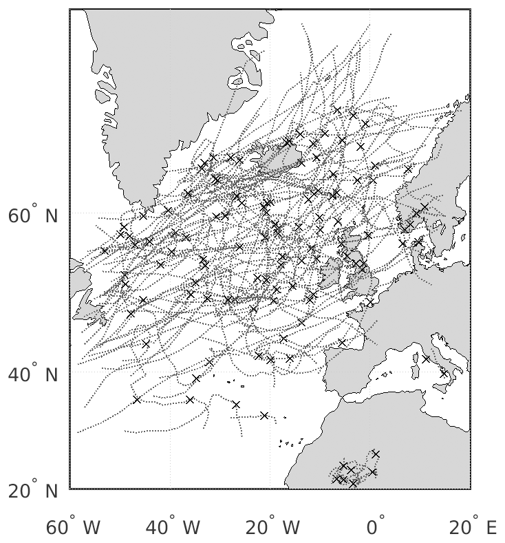
Figure 1Mercator projection of the area covered, with all 139 cyclone tracks found by the algorithm. Crosses indicate the location of minimum sea level pressure along each track.
Composites of extratropical cyclones
Ultimately, we want to analyse the variability of the tropopause inversion layer within extratropical baroclinic waves. For this, we compute composites of the cyclones at the time of maximum intensity, which we define as the occurrence of the global minimum surface pressure along the track. We select a subset of the gridded data as provided by the ECMWF for each cyclone by rotating the pole of a spheric polar coordinate system (Θ, ϕ) onto the centre of the cyclone and interpolated the original data onto that new grid. The horizontal resolution of the new coordinate system is set to 0.25∘ and the spherical cap radius to ∘. The radius is chosen such that all relevant features around the cyclone centre are covered. Figure 2 illustrates the interpolation of the data from the original latitude–longitude grid provided by the ECMWF (light grey area for the whole sphere, dark grey for the limited area used in this study) onto an arbitrarily placed new spherical polar coordinate system (orange area). The rotation of the new coordinate system onto the cyclone centre is performed following Bengtsson et al. (2007), who provide a detailed description of the rotation matrix in their appendix. The original ECMWF IFS variables in latitude–longitude coordinates are interpolated onto a column covered by the new coordinate system, with the vertical coordinate using the lapse-rate-based tropopause as a reference altitude (Birner, 2006). The tropopause height is defined as zero with negative (positive) height values below (above) and a vertical grid spacing of Δz=100 m. The interpolation onto the new coordinate system based on the centre of the surface cyclone does not account for a potential vertical tilt of the cyclone. However, since this study focusses on the point in time of maximum cyclone intensity when the vertical structure tends to align, we find a tilt to be negligible. The ensemble of tropopause-based columns of variables from each cyclone is then averaged to create a three-dimensional composite of the flow in the vicinity of the cyclones. Subsequently, the mean absolute height coordinate is recovered as follows. Each horizontal coordinate (Θ, ϕ) of each individual cyclone within the new coordinate system still carries the information about the absolute tropopause height at that location, and therefore a mean tropopause height can be calculated and assigned to that horizontal location within the composite.

Figure 2Schematic of the size of the analysed region (dark grey) in comparison to the full sphere, as well as the size of a rotated spheric polar coordinate system (orange) with ∘ radius. The dark grey semi-transparent upright plane illustrates (with exaggerated vertical extent) the vertical cross section aligned from north to south as displayed in Fig. 9.
In the special case of composites of horizontal or quasi-horizontal fields like PV on isentropes or the TIL strength, we first calculate the fields for each cyclone and then afterwards the mean. This method preserves more information because the three-dimensional tropopause-based averaging still smoothes vertical information due to the variability of, for example, the height of the maximum in N2 above the tropopause. In contrast to other studies analysing cyclone composites (e.g. Bengtsson et al., 2007; Catto et al., 2010), we keep the orientation of each individual cyclone instead of rotating them depending on their path of migration. In our case this approach leads to a better representation of the dynamical and thermodynamical features in the UTLS.
Before we present the results of the cyclone composites, we first discuss two cases of individual cyclones and associated TIL evolution over the North Atlantic. We choose these cases since both cyclones are associated with upper tropospheric baroclinic wave-breaking events very similar to the ones described in idealised baroclinic life cycle simulations. The first case study shows an evolution comparable to an LC2 (life cycle 2), while the second one exhibits the distinct features of an LC1 (life cycle 1) wave-breaking event (Thorncroft et al., 1993). Although the waves occur consecutively in time and space, they are not interacting directly and the cyclones at surface level evolve relatively isolated from each other, in contrast to multi-cyclone-centres as described for example by Hanley and Caballero (2012).
3.1 Baroclinic wave with LC2 characteristics
Figure 3 shows three consecutive time steps of the evolution of the first baroclinic wave with the time of maximum intensity depicted in the second row. We focus our analysis and discussion on the flow features inside the 15∘ radius around the cyclone centre. Furthermore, we focus our discussion on sea level pressure, isentropic potential vorticity (IPV) at 330 K, strength of the tropopause inversion layer as defined in the beginning of Sect. 2, and relative vorticity at the lapse rate tropopause (from left to right in Fig. 3).
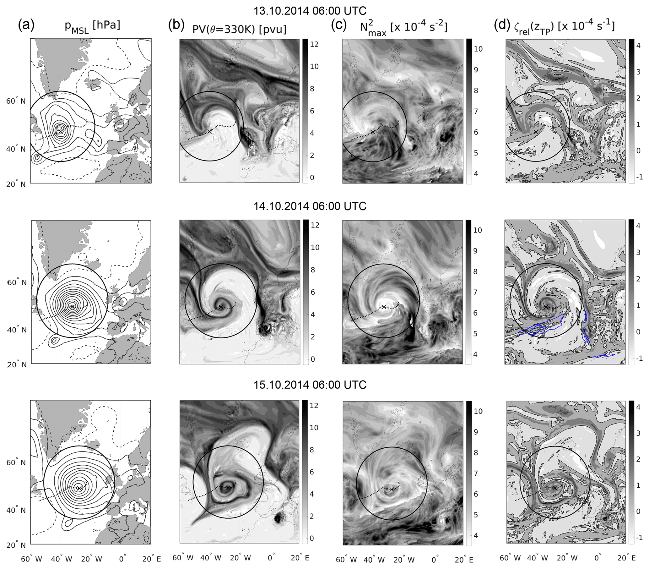
Figure 3Evolution of a baroclinic wave-breaking event as seen in ECMWF IFS analysis data. The middle row represents 14 October 2014 at 06:00 UTC (the point in time of maximum cyclone intensity), and the upper and lower row show the situation 24 h prior and past the maximum intensity. Column (a) shows the pressure at mean sea level (solid lines pmsl≤1013 hPa, dashed lines pmsl>1013 hPa, in steps of 5 hPa), (b) the IPV on 330 K, (c) the maximum of static stability within 3 km above the thermal tropopause as an indicator for the TIL strength, and (d) the relative vorticity at lapse rate tropopause height. Blue lines in the middle row show 40 and 50 m s−1 horizontal wind speed isolines at 200 hPa. The dashed black line shows the path of migration of the tracked cyclone, with the position of the cyclone centre at the point in time of the meteorological field displayed marked by the black ×. Black circles show the 15∘ radius used for the composites. Note the deformation of the circles due to the mercator projection.
A total of 24 h before the cyclone reaches maximum intensity the MSL pressure already falls below 975 hPa. The IPV shows a baroclinic wave centred above the tracked surface cyclone centre, with large IPV values coming from high latitudes and tilting in the northwest–southeast direction into the jet. During the intensification of the surface cyclone, the upper air wave enters what Thorncroft et al. (1993) call the cyclonic wrap-up phase, which in this case study exhibits the distinct features of an LC2. During the wrap-up, which is vertically aligned with the strong surface cyclone, the trough stays on the northern cyclonic shear side of the jet streak as indicated by the 200 hPa horizontal wind maximum in Fig. 3d. The wave-breaking event is meridionally confined by the jet streak and only a very thin streamer of enhanced IPV air turns anticyclonically on the last day depicted in Fig. 3.
The relative vorticity at lapse rate tropopause height correlates with the IPV where cyclonic (anticyclonic) flow exhibits large (low) values of IPV. The regions with relatively small (large) values of IPV and anticyclonic (cyclonic) flow exhibit enhanced (reduced) values of static stability above the tropopause. This correlation especially holds true inside the 15∘ radius area and at the point in time of maximum cyclone intensity. This agrees well with the anticipated role of balanced dynamics (Wirth, 2003, 2004) and idealised baroclinic life cycle simulations with a focus on the evolution of the TIL (e.g. Erler and Wirth, 2011). It furthermore agrees with the measurement-based study by Pilch Kedzierski et al. (2015) concerning the correlation between the upper tropospheric relative vorticity and the static stability above the tropopause within troughs and ridges. The regions with the largest values of static stability up to s−2 are located inside the ridge in the first time step and later in the second time step in the tropospheric IPV air mass which is wrapped up around the underlying cyclone centre. In the last time step, the TIL strength especially within the 15∘ radius reverts to lower values. We want to highlight the fact that the enhancement of the TIL strength during the wave-breaking event is not uniform, but rather shows a large spatial variability and wave-like patterns on different horizontal scales. The regions with the strongest enhancement of static stability above the tropopause in the second time step depicted in Fig. 3, as well as inside the deformed ridge in the third time step, are associated with the regions commonly affected by the warm conveyor belt (Madonna et al., 2014). The connection between the warm conveyor belt outflow and the regions of enhanced static stability above the tropopause is also a feature of the baroclinic life cycle simulations by Kunkel et al. (2016).
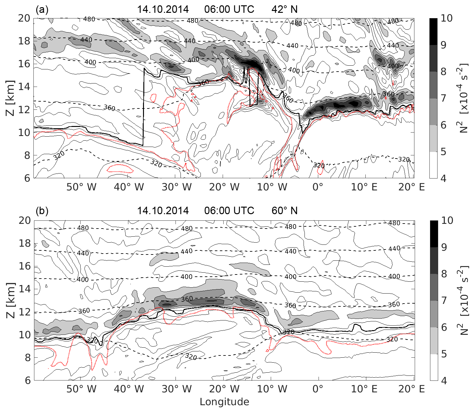
Figure 4Vertical cross section over the North Atlantic on 14 October 2014 at 06:00 UTC (a) at 42∘ N and (b) at 60∘ N. The filled contour as well as the thin solid black contour lines show static stability N2 in steps of s−2, dashed black lines show isentropes. The bold solid black line indicates the lapse rate tropopause, the dotted red line shows the 2 pvu isoline of potential vorticity.
The TIL strength at lower latitudes in the quasi-horizontal illustration (Fig. 3c) sometimes exhibits strong gradients or jumps which appear non-coherent. These strong gradients are an artefact of the evaluation, due to (1) the restriction of the TIL strength to the global maximum in static stability within 3 km above the lapse rate tropopause, (2) the high variability of the tropopause defining lapse rate in the high-resolution data, (3) the occurrence of sharp tropopause jumps and double tropopauses (especially during wave-breaking events), and (4) the strongly structured TIL itself. The occurrence of such features should be kept in mind when analysing such synoptic situations in a high-resolution data set. We compared such prominent structures in the quasi-horizontal illustration of the TIL with a variety of vertical cross sections, to ensure that the statements we make about the TIL evolution hold true and are in fact not a numerical evaluation artefact. Figure 4a shows an example for a vertical cross section corresponding to the second time step depicted in Fig. 3 and at 42∘ N. It illustrates the large variability of the three dependent variables PV, static stability N2, and the lapse rate tropopause height. The jump of the lapse rate tropopause at about 37∘ W as well as the small-scale stratospheric PV intrusion at about 12∘ W illustrate the complexity of the tropopause location and the challenge to account for this by the different definitions of the tropopause and the TIL. The vertical cross section in Fig. 4b shows the TIL structures at 60∘ N on the same day and north of the cyclone centre. It illustrates that the regions of enhanced static stability exhibit less variability at this latitude. They are located above the ridge between 40 and 10∘ W, with the wave-like horizontal pattern that is also visible in Fig. 3c.
3.2 Baroclinic wave with LC1 characteristics
Figure 5 shows the subsequent baroclinic wave-breaking event 3 d later over the North Atlantic. The MSL pressure on 16 October still shows two distinct minima: the decaying northern one associated with the previous wave-breaking event, and a newly formed minimum. The background state of the UTLS is still significantly distorted due to the LC2 wave-breaking event described in Sect. 3.1. Similar to the previous case, a relatively small scale baroclinic wave is evident in the IPV field above the underlaying surface cyclone centre. In contrast to the previous case, as the surface cyclone grows stronger and the upper air wave enters the wrap-up phase (Fig. 5, middle row), the initially cyclonically tilted trough with enhanced values of IPV turns anticyclonically and later on a substantial part of the trough penetrates the jet in its excursion southwards. The jet splits into two jet streaks (Fig. 5d, middle row) and the trough gets thinned, eventually producing a cut-off (Fig. 6). These wave-breaking characteristics meet the definition of an LC1 as described by Thorncroft et al. (1993). During the evolution of the cyclone the relations between tropospheric IPV, anticyclonic relative vorticity at tropopause height, and an enhancement in static stability above the tropopause are all evident. The regions of maximum static stability with values up to s−2 are again located inside the ridge of low IPV air wrapping up around the underlaying cyclone centre at about the time of maximum cyclone intensity. The thinning and southward-moving trough itself exhibits low values of static stability N2 above the tropopause, in agreement with its positive relative vorticity, but the flow around the trough shows no distinct strong signal in the quasi-horizontal static stability distribution, especially when compared to the cyclonic wrap-up 24 h earlier.
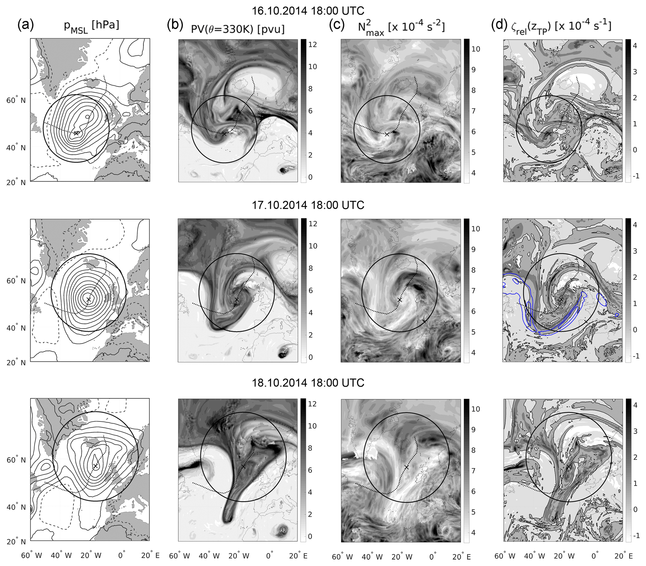
Figure 5As in Fig. 3, but for the subsequent cyclone with maximum intensity on 17 October 2014 at 18:00 UTC, depicted in the middle row. Top row shows 24 h earlier and bottom row 24 h later.

Figure 6As in Fig. 3, but only for one point in time, showing the tracked cyclone associated with the upper tropospheric cut-off from the previous baroclinic wave breaking.
Figure 6 shows a comparable evolution about two days later for the secondary cyclone associated with the cut-off which formed from the thinning streamer. This cyclone was also tracked by the algorithm, and, while it is weaker and exhibits less horizontal extent than the two previous cases, the region of maximum static stability with values of up to s−2 still evolves inside the wrapped-up low-IPV air. The wrapped-up cut-off exhibits maximum static stability values of about s−2. The regions of high static stability above the tropopause are located north of the cyclone centre inside the flow with negative relative vorticity, as well as inside the flow that turns anticyclonically northwest of the cyclone centre and towards the jet maximum (as indicated by the blue contour lines in Fig. 6d).
In conclusion, we analysed two subsequent baroclinic life cycles, the first resembling an LC2, and the second an LC1 when compared with idealised baroclinic life cycle simulations. In both cases the regions of strongest enhancement in static stability above the tropopause are located inside the ridge of low-IPV air moving northward from low latitudes and wrapping up around the underlaying primary cyclone about the time of maximum cyclone intensity. The flow around the southward excursion of the trough in the LC1 wave exhibits no distinct signal, until a secondary cyclone associated with the cut-off from the trough evolves. This cyclone-linked behaviour can also be seen in the idealised baroclinic life cycle simulations from Erler and Wirth (2011). Their Fig. 4 shows a comparable evolution of the TIL strength with consideration that there are two northern surface cyclone intensification periods and one cut-off related cyclone forming at low latitudes.
Based on the analysis of these two case studies, we further motivate the analysis of the evolution of the TIL during baroclinic life cycles based on the flow above surface cyclones. We recognise that surface cyclones exist which are not linked to baroclinic wave-breaking events and also baroclinic wave-breaking events (in the sense of meridional irreversible redistribution of isentropic potential vorticity) exist which are not linked to surface cyclones. Nevertheless, we expect a composite of strong surface cyclones to give a characteristic representation of the flow where a strong TIL forms during the subset of those baroclinic wave-breaking events which are in fact linked to surface cyclones.
In the following section we present composites to define a mean characteristic evolution of the flow features in the UTLS above surface cyclones during baroclinic wave-breaking events. We compute composites of subsets of the tracked cyclones based on the surface cyclone strength, because we expect the strength to be a good indicator for the amount of coupling between the surface cyclone and the flow in the UTLS. We abstain from presenting composites from cyclone subsets based on other criteria because the amount of cyclones tracked in our data set quickly reduces to a statistically non-significant amount when specific criteria are applied.
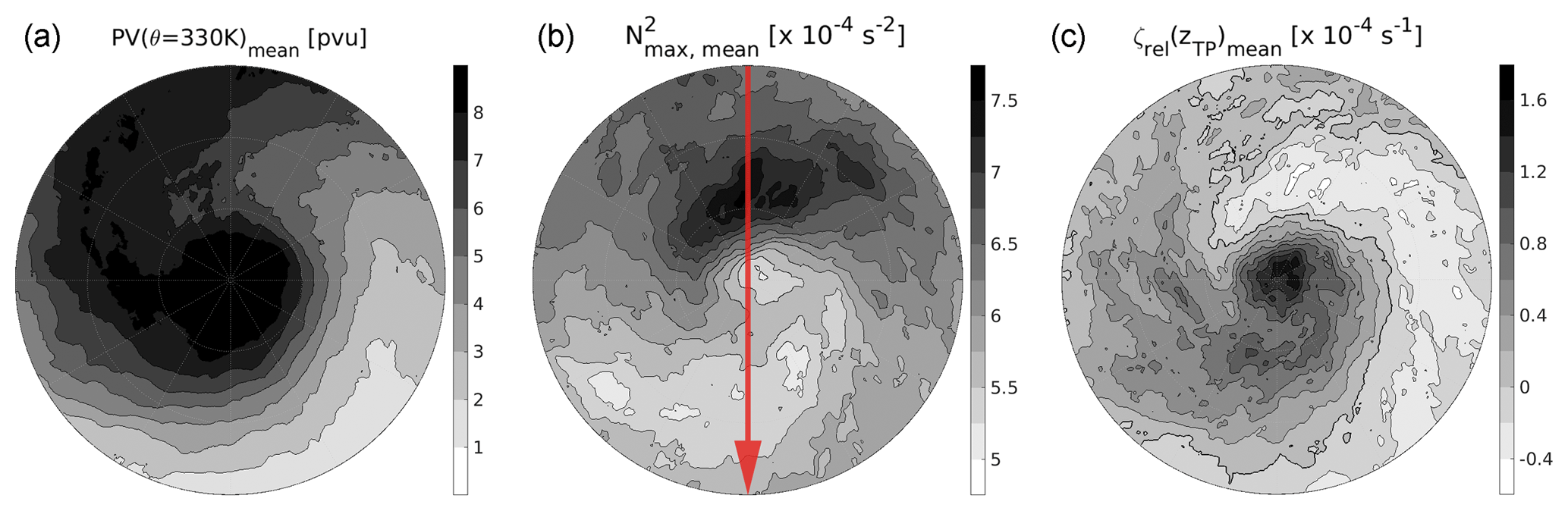
Figure 7Composite of flow features for the 76 strong cyclones with hPa at the point in time of maximum intensity: (a) IPV on 330 K, (b) TIL strength , and (c) relative vorticity ζrel at lapse rate tropopause height. The ζrel=0 s−1 isoline is indicated by the black solid line. The red arrow in the middle indicates the orientation of the cross section in Fig. 9.
Figure 7 shows the quasi-horizontal composites of selected features from the 76 strong cyclones with hPa. The three contour plots show a mean state of the UTLS flow, which is broadly comparable to the two case studies of baroclinic wave-breaking events discussed previously. The first contour plot shows a streamer of stratospheric IPV on 330 K reaching from the northwest into the cyclone centre, with a cyclonic rotational component. Naturally, the lowest values of IPV are located in the south and gradually approach the IPV values of the stratospheric streamer when rotating counterclockwise around the cyclone centre along the wrap-up. This region of strong tangential gradients of IPV (with respect to the cyclone centre) exhibits for the most part a negative mean relative vorticity at tropopause height and also large values of static stability in the lower stratosphere. The maximum values of static stability are located north of the cyclone centre with maximum values up to s−2. The stratospheric IPV streamer as well as the southern regions of strong radial IPV gradients exhibit a cyclonic relative vorticity at tropopause height as well as a relatively weak TIL with values of about ≈ (5–5.5) × 10−4 s−2.
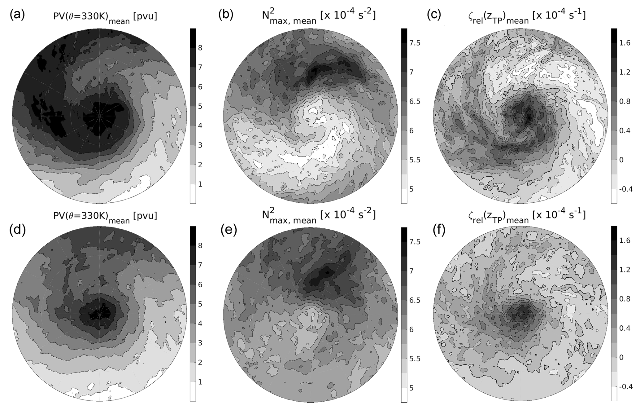
Figure 8As in Fig. 7, but for (1) panels (a)–(c): for the 30 very strong cyclones with hPa, and (2) panels (d)–(f): the 54 weak cyclones with hPa.
In Fig. 8 the same contour plots are displayed for a subset of very strong cyclones as well as a subset of weak cyclones. The composites in the top row represent the 30 very strong cyclones with hPa. The dominating cyclonic rotational component is more pronounced and the air masses with distinctly different features are wrapped up around the cyclone centre to a larger degree. The relative vorticity and the TIL strength still correlate well and their horizontal gradients are sharper compared to those in Fig. 7. The latter is not caused by a stronger TIL in the case of hPa, but more due to a clearer separation and also a significant decrease in TIL strength in the cyclonic flow. The 54 weak cyclones with hPa are presented in Fig. 8d–f. The features described for the subsets of the strong and the very strong cyclones are still evident, however, with smoother gradients in all three features depicted and a weaker separation between tropospheric and stratospheric (influenced) air masses. The region of maximum enhancement of static stability above the tropopause is still located north of the cyclone centre and also still reaches mean values of about ≈ (7–7.5) × 10−4 s−2.
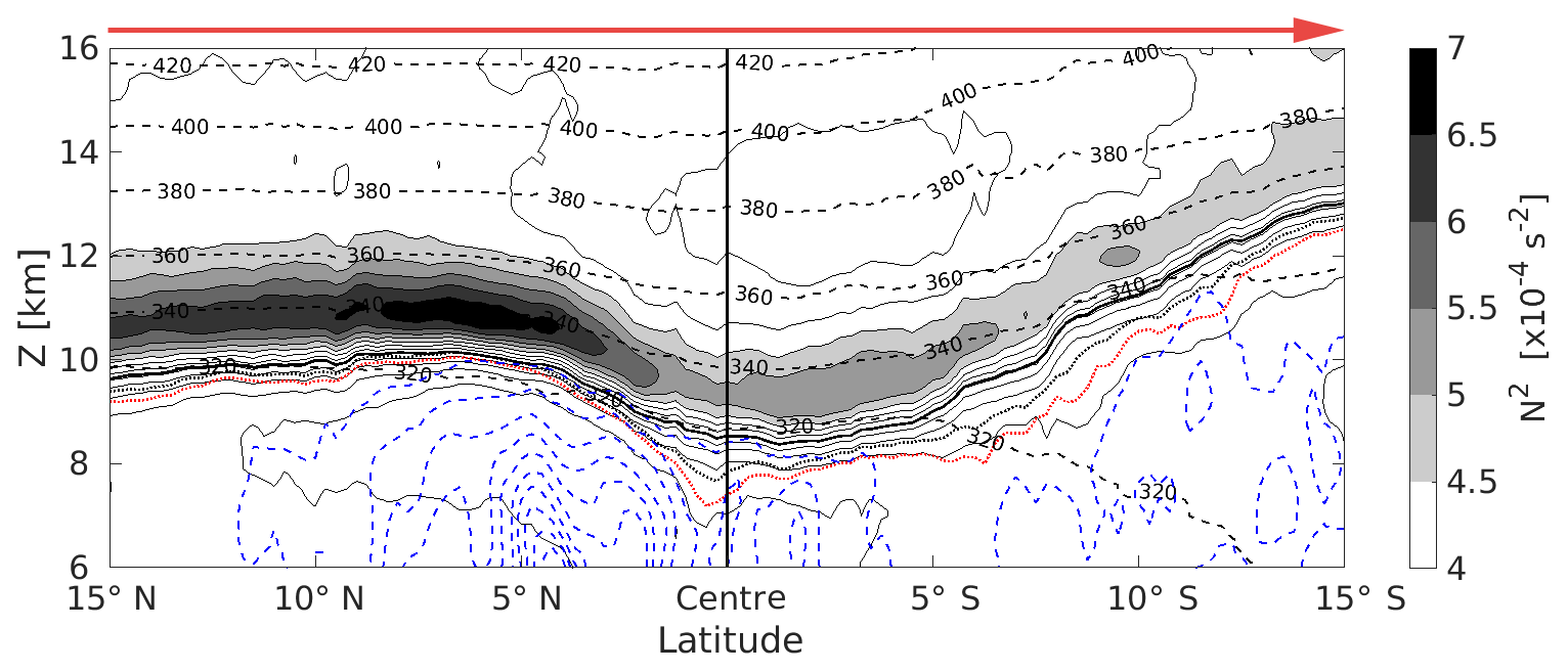
Figure 9Vertical cross section of the mean state from the 76 strong cyclones, from north to south through the centre of the cyclone, as indicated by the red arrow here and in Fig. 7b. The cross section is composed of the tropopause-based mean of vertical profiles at each latitude. The mean tropopause height has been restored. Filled contour as well as solid black contour lines show static stability N2 in steps of s−2, dashed black lines isentropes, and dashed blue lines the cloud ice water content (ciwc), with the first isoline at kg kg−1 and steps of the same value. The bold solid black line indicates the lapse rate tropopause, the dotted red (black) line the 2 pvu (2.5 pvu) isoline of potential vorticity, indicating near-tropopause PV gradients.
Figure 9 shows a mean vertical cross section from north to south through the cyclone centre for the 76 strong cyclones with hPa along the red line as indicated in Fig. 7. The thermal and dynamical tropopauses both exhibit minimum height in the cyclone centre and both slope upward south of the cyclone centre. Furthermore, the regions of maximum TIL strength partly align vertically above regions of ascending air and cloud formation in the troposphere, indicated by the cloud ice water reaching up to the lapse rate tropopause. This hints towards the role of moist dynamical processes in the formation of the TIL (Kunkel et al., 2016). To analyse the region of strongest enhancement in static stability north of the cyclone centre in more detail, we derive the composites shown in Fig. 10. Depicted are the vertical wind, the squared vertical shear of the horizontal wind S2, and the gradient Richardson number, similar to the northern half of the cross section in Fig. 9 for the same subset of cyclones ( hPa). The mean vertical wind ω correlates well with the mean cloud ice water content. The ice clouds within and above the strong tropospheric updraft north of the cyclone centre, reaching up to the tropopause with potential temperatures over Θ=320 K, are features of the region where the warm conveyor belt outflow typically occurs (e.g. Madonna et al., 2014). The stratosphere shows no distinct mean vertical velocity signal and the troposphere far north from the cyclone centre exhibits slowly descending air masses. The squared vertical shear of the horizontal wind speed shows a maximum above the tropopause, with a remarkable overlap into the regions of maximum static stability. Based on these results, we calculate the dimensionless gradient Richardson number Ri. It is defined as the ratio of static stability N2 and the vertical shear of the horizontal wind S2, . Enhanced values of N2 describe a stably stratified flow with suppressed vertical motion, while enhanced vertical shear of the horizontal wind can result in dynamical shear instability. Linear wave theory predicts a critical Richardson number of Ric=0.25, where dynamic instability can develop in stably stratified flow with Ri<Ric. We calculate the modified Richardson number mean as described in Birner et al. (2002), who take the natural logarithm of the individual Richardson numbers before computing an average to reduce the variability range: . The mean Richardson number is then calculated as . The result is depicted in Fig. 10 and shows two regions of minimum mean Richardson numbers. The lowest values of Ri are evident in the upper troposphere in the upper regions of the ascending air masses, which is a result of a very weak stratification combined with a moderately strong vertical wind shear due to a local maximum of the meridional wind component at tropopause height at about 7.5∘ N (not shown). A second region of minimum mean Richardson numbers is located right above the tropopause near the cyclone centre and extends into the regions of maximum static stability. In this region the vertical wind shear S2 is the dominating factor that works towards dynamic instability. This agrees well with one result from Birner et al. (2002), who saw a similar partly vertical overlap of a maximum in vertical wind shear and the TIL in radiosonde profiles. Grise et al. (2010) furthermore stated a fundamental link between the zonal-mean static stability and the zonal-mean zonal wind based on the thermal wind relation, highlighting a dependency between the meridional gradient of the static stability and the curvature of the vertical shear of the horizontal wind.
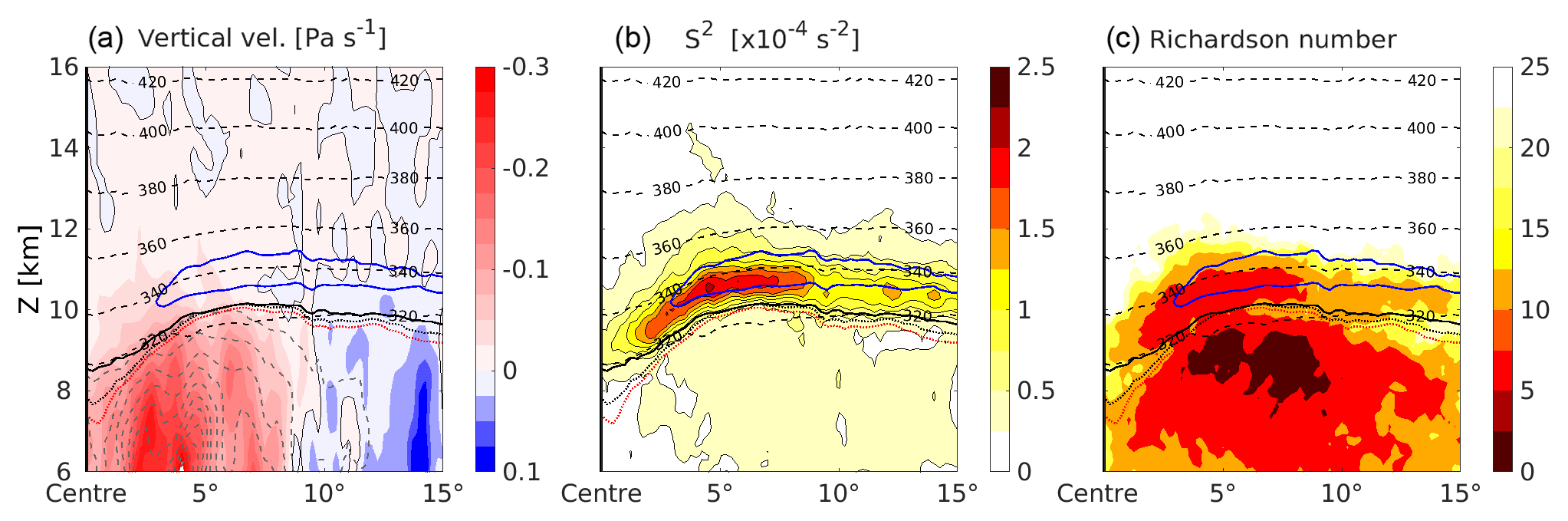
Figure 10Vertical tropopause-based averaged cross section as in Fig. 9, but only north of the cyclone centre. (a) Filled contours show mean vertical velocity, solid thin black line the ω=0 Pa s−1 isoline. Grey dashed lines are isolines of the cloud ice water content, steps as in Fig. 9. (b) Filled contour and solid black contour lines show squared vertical shear of horizontal wind S2. (c) Modified Richardson number mean Ri, with an inverted colour scale (red represents low values) to highlight the tendency toward turbulent motion. Blue solid bold line in all three panels shows the s−2 isoline, dashed black lines the isentropes.
We furthermore tested different methods of calculating an average Richardson number to check the robustness of our result. Calculating the unmodified Richardson numbers for each individual cyclone and averaging afterwards produces a very fragmented mean field, but it still exhibits a region with local minima of the order of 101 inside the region of the TIL. Calculating the mean Richardson number from the averaged potential temperature and wind field yields a result more comparable to the modified Richardson mean, but with overall larger values for Ri, stronger separated minima, and sharper gradients of Ri. Birner et al. (2002) observed a distinct discrepancy in the vertical shear of the horizontal wind S2 above the tropopause between the radiosonde data and ECMWF reanalysis data. This shows that the vertical wind gradients in the UTLS are not well resolved and are significantly underestimated by the reanalysis data, a tendency which might still be the case in the analysis data. The fact that we see a strong maximum in S2 above the tropopause in NWP data, while Birner et al. (2002) saw none in the mean profiles from reanalysis data, can be explained by (1) the finer vertical and horizontal resolution in the operational IFS model, and (2) the fact that we present a composite of a specific synoptic situation which may result in a similar structure of the individual vertical profiles. The lowermost stratosphere north of the cyclone centre exhibits Richardson numbers of , which are still well above the critical value of Ric=0.25 for turbulent flow. These Richardson numbers, however, present an average over 76 cyclones. For individual cyclones, Richardson numbers often exhibit much lower values in this region, including instances below the critical value Ric, and thus are indicative of the possibility of dynamic instability. Also we would like to remind the reader that these quantities are derived from model data with a vertical grid spacing of about Δz≈300 m. The two features of interest ( and ) typically exhibit a vertical extent of 1–3 km, and therefore the model output profiles of N2 and S2 in the lowermost stratosphere can be expected to be a somewhat smoothed representation of the real atmosphere. A possible misrepresentation of the ratio between the two gradient-based measures N2 and S2 opens the possibility for an even larger range of Richardson numbers in the real flow. In conclusion, there is the possibility that turbulence is present even in regions of enhanced static stability in the lower stratosphere, which might affect cross tropopause transport in these regions.

Figure 11Composite of the vertical wind shear for the 76 strong cyclones with hPa at the point in time of maximum intensity, averaged over the individual quasi-horizontal fields of maximum vertical wind shear found within 3 km above the lapse rate tropopause for each cyclone. The black arrows indicate the orientation of the vertical cross sections in Fig. 12.
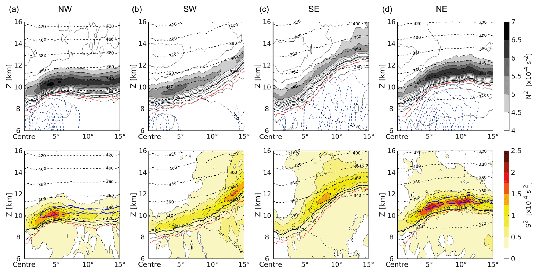
Figure 12Composites of flow features for the 76 strong cyclones with hPa at the point in time of maximum intensity. Vertical tropopause-based averaged cross section composites, reaching from the cyclone centre (a) northwestward, (b) southwestward, (c) southeastward and (d) northeastward. Top row shows static stability N2 and cloud ice water content as in Fig. 9, bottom row shows wind shear S2 as in Fig. 10b. The orientation of the vertical cross sections is indicated by the black arrows in Fig. 11.
Figure 11 further illustrates the connection between the regions of enhanced static stability and the vertical shear of the horizontal wind in the vicinity of cyclones. It shows the composite derived from the quasi-horizontal fields of maximum wind shear found within 3 km above the tropopause in the 76 strong cyclones. The region of largest mean wind shear matches with the region of maximum enhanced static stability (see Fig. 7b), with maximum values north and northeast of the cyclone centre within the wrapped-up ridge. The southern regions exhibit weaker mean wind shear, and the minimum values of are located around the cyclone centre.
Figure 12 shows tropopause-based averaged vertical cross sections that cover the distance from the cyclone centre to the spherical cap radius of 15∘ and are oriented in different cardinal directions as indicated in Fig. 11. These plots complement Figs. 10b and 11 and further confirm a co-location as well as a co-occurrence of the regions of maximum wind shear and the regions of maximum enhanced static stability . They furthermore illustrate the validity and representativity of the composites derived from the individual quasi-horizontal fields. The quasi-horizontal composite in Fig. 7b strongly depends on the definition of the TIL strength (in this case the maximum value of N2 within 3 km above the tropopause), while the vertical cross section composites in the top row of Fig. 12 solely depend on the tropopause definition. However, both methods show a good agreement, aside from an overall shift of the absolute values, as expected and described in Sect. 2.2.1. The same comparison can be made between Fig. 11 and the bottom row of 12 for the vertical shear of the horizontal wind S2. Overall the composites give a comprehensive overview of the mean evolution of the TIL above surface cyclones and its relation with other flow features like tropospheric moist diabatic active regions or wind shear in the lower stratosphere.
The goal of this study was to analyse the development of the TIL during the evolution of baroclinic life cycles in operational ECMWF IFS analysis data. For this we tracked a total sum of 130 surface cyclones in the MSL pressure field over the North Atlantic from August to October during a 5-year period from 2010 to 2014. We presented an analysis of two consecutive individual cyclones associated with two upper tropospheric baroclinic wave-breaking events, one resembling an LC1 and the other one an LC2 event. We furthermore derived composites of the atmospheric state from different subsets of the 130 cyclones using the intensity of the surface cyclone as a selection criterion.
Based on the analysis of the two individual baroclinic life cycles (Sect. 3) in comparison with idealised baroclinic life cycle simulations from previous works (Wirth and Szabo, 2007; Erler and Wirth, 2011; Kunkel et al., 2014, 2016), we identified the regions of cyclonic wrap-up around the cyclone centre as the regions exhibiting the strongest signal in static stability above the lapse rate tropopause. The flow in the UTLS with relatively large values of isentropic potential vorticity and positive relative vorticity coming from northwest and wrapping up around the cyclone centre exhibits low values of static stability, while the counterpart of anticyclonic low-IPV air originating from lower latitudes shows a distinct enhancement in static stability and represents the region with a well-developed TIL. The largest values of static stability above the tropopause are located north and northeast of the cyclone centre at about the time of maximum surface cyclone intensity. The synoptic-scale TIL evolution in both the LC1 and LC2 baroclinic waves is similar, with differences in the strength and the shape of the region of the wrap-up. The relatively weak secondary cyclone associated with the cut-off which resulted from the LC1 wave-breaking event shows a similar evolution on a smaller horizontal scale. The TIL above the individual cyclones exhibits a large temporal, horizontal, and vertical variability on different scales associated with the variety of known forcing mechanisms being resolved in the high-resolution NWP data.
Furthermore, we presented composites of the atmospheric state in the vicinity of different subsets of tracked cyclone centres at the point in time of maximum cyclone intensity. We find that stronger surface cyclones are associated with a sharper and more pronounced wrap-up in the UTLS flow. The composites furthermore resemble to a large degree the key features of the TIL evolution and the mean flow as identified from the case studies. The regions of largest TIL enhancement are located north and northeast of the cyclone centre, above regions influenced by strong tropospheric updrafts and clouds reaching up to the tropopause, where in this central stage of the baroclinic life cycle the warm conveyor belt outflow typically occurs (e.g. Madonna et al., 2014; Kunkel et al., 2016). The presence of high clouds supports the hypothesised importance of moist dynamical and radiative processes during the formation of the TIL (e.g. Randel et al., 2007; Kunkel et al., 2016). The composites further reveal a maximum in vertical shear of the horizontal wind S2 within the region of strongest enhancement of static stability above the tropopause. The regions of maximum static stability and those of maximum wind shear show a remarkable overlap, horizontally as well as vertically, which is in agreement with previous studies (Birner et al., 2002; Grise et al., 2010). Mean Richardson numbers calculated for these flow conditions reveal a region of local minima in Ri right above the tropopause at around 5∘ north from the cyclone centre in the composite. Taking into account the variability of N2 and S2 for individual cyclones, this result points toward the possibility of a co-location between enhanced static stability above the tropopause and localised regions of turbulent mixing of tropospheric and stratospheric air masses (Kunkel et al., 2016).
We want to note that baroclinic life cycles vary in their appearance from case to case and thus the TIL evolution in individual cyclones can differ from the one described by the composite analysis. The analysis of baroclinic life cycles in other regions and seasons would of course be desirable, but is left open at this stage for later studies. The approach used in this study is now applicable to a large data set, e.g. using the new ERA-5 reanalysis which has the same vertical resolution in the UTLS as the analysis data in this study.
Overall this study confirms the importance of baroclinic waves and their embedded cyclones to explain the meso-scale variability of enhanced static stability above the lapse rate tropopause in the extratropics. The high spatial and temporal resolution of the analysis data gives a better understanding on where and when static stability increases during baroclinic life cycles. The composites of baroclinic life cycles show a large agreement of TIL evolution with the individual life cycles in the analysis data as well as with the individual life cycles from earlier idealised studies (Erler and Wirth, 2011; Kunkel et al., 2016). They furthermore indicate that turbulent mixing might occur in regions of enhanced static stability right above the tropopause.
ECMWF operational analysis data have been retrieved from the MARS server. Output from the tracking algorithm and the projection of the atmospheric field variables on the rotated grids is available upon request (kaluzat@unimainz.de).
DK, PH, and TK designed the research project. TK developed the model code, performed the calculations, and analysed the data with the help of DK and PH. TK prepared the paper with contributions from all authors.
The authors declare that they have no conflict of interest.
The authors acknowledge funding from the German Science Foundation, as this study was carried out as part of the preparation phase for the WISE campaign under funding from the HALO SPP 1294. We are furthermore grateful to the ECMWF for providing the IFS analysis data which have been downloaded from the ECMWF MARS system.
This research has been supported by the Deutsche Forschungsgemeinschaft (grant nos. KU 3524/1-1, HO 4225/7-1, and HO 4225/8-1).
This paper was edited by Amanda Maycock and reviewed by two anonymous referees.
Bengtsson, L., Hodges, K. I., Esch, M., Keenlyside, N., Kornblueh, L., Luo, J. J., and Yamagata, T.: How may tropical cyclones change in a warmer climate?, Tellus A, 59, 539–561, https://doi.org/10.1111/j.1600-0870.2007.00251.x, 2007. a, b
Birner, T.: Fine-scale structure of the extratropical tropopause region, J. Geophys. Res.-Atmos., 111, 1–14, https://doi.org/10.1029/2005JD006301, 2006. a, b, c
Birner, T.: Residual Circulation and Tropopause Structure, J. Atmos. Sci., 67, 2582–2600, https://doi.org/10.1175/2010JAS3287.1, 2010. a
Birner, T., Dörnbrack, A., and Schumann, U.: How sharp is the tropopause at midlatitudes?, Geophys. Res. Lett., 29, 45-1–45-4, https://doi.org/10.1029/2002GL015142, 2002. a, b, c, d, e, f, g
Catto, J. L., Shaffrey, L. C., and Hodges, K. I.: Can climate models capture the structure of extratropical cyclones?, J. Climate, 23, 1621–1635, https://doi.org/10.1175/2009JCLI3318.1, 2010. a, b
Cressman, G. P.: An Operational Objective Analysis System, Mon. Weather Rev., 87, 367–374, https://doi.org/10.1175/1520-0493(1959)087<0367:AOOAS>2.0.CO;2, 1959. a
Erler, A. R. and Wirth, V.: The Static Stability of the Tropopause Region in Adiabatic Baroclinic Life Cycle Experiments, J. Atmos. Sci., 68, 1178–1193, https://doi.org/10.1175/2010JAS3694.1, 2011. a, b, c, d, e, f, g
Flaounas, E., Raveh-Rubin, S., Wernli, H., Drobinski, P., and Bastin, S.: The dynamical structure of intense Mediterranean cyclones, Clim. Dynam., 44, 2411–2427, https://doi.org/10.1007/s00382-014-2330-2, 2015. a
Gettelman, A. and Wang, T.: Structural diagnostics of the tropopause inversion layer and its evolution, J. Geophys. Res.-Atmos., 120, 46–62, https://doi.org/10.1002/2014JD021846, 2015. a, b
Gisinger, S., Dörnbrack, A., Matthias, V., Doyle, J. D., Eckermann, S. D., Ehard, B., Hoffmann, L., Kaifler, B., Kruse, C. G., Rapp, M., Gisinger, S., Dörnbrack, A., Matthias, V., Doyle, J. D., Eckermann, S. D., Ehard, B., Hoffmann, L., Kaifler, B., Kruse, C. G., and Rapp, M.: Atmospheric Conditions during the Deep Propagating Gravity Wave Experiment (DEEPWAVE), Mon. Weather Rev., 145, 4249–4275, https://doi.org/10.1175/MWR-D-16-0435.1, 2017. a
Grise, K. M., Thompson, D. W., and Birner, T.: A global survey of static stability in the stratosphere and upper troposphere, J. Climate, 23, 2275–2292, https://doi.org/10.1175/2009JCLI3369.1, 2010. a, b
Hanley, J. and Caballero, R.: Objective identification and tracking of multicentre cyclones in the ERA-Interim reanalysis dataset, Q. J. Roy. Meteor. Soc., 138, 612–625, https://doi.org/10.1002/qj.948, 2012. a, b, c, d, e
Hegglin, M. I., Boone, C. D., Manney, G. L., and Walker, K. A.: A global view of the extratropical tropopause transition layer from Atmospheric Chemistry Experiment Fourier Transform Spectrometer O3, H2O, and CO, J. Geophys. Res.-Atmos., 114, 1–18, https://doi.org/10.1029/2008JD009984, 2009. a, b
Hoor, P., Fischer, H., Lange, L., Lelieveld, J., and Brunner, D.: Seasonal variations of a mixing layer in the lowermost stratosphere as identified by the CO-O3 correlation from in situ measurements, J. Geophys. Res.-Atmos., 107, ACL 1-1–ACL 1-11, https://doi.org/10.1029/2000JD000289, 2002. a
Hoor, P., Gurk, C., Brunner, D., Hegglin, M. I., Wernli, H., and Fischer, H.: Seasonality and extent of extratropical TST derived from in situ CO measurements during SPURT, Atmos. Chem. Phys., 4, 1427–1442, https://doi.org/10.5194/acp-4-1427-2004, 2004. a
Kunkel, D., Hoor, P., and Wirth, V.: Can inertia-gravity waves persistently alter the tropopause inversion layer?, Geophys. Res. Lett., 41, 7822–7829, https://doi.org/10.1002/2014GL061970, 2014. a, b, c, d
Kunkel, D., Hoor, P., and Wirth, V.: The tropopause inversion layer in baroclinic life-cycle experiments: the role of diabatic processes, Atmos. Chem. Phys., 16, 541–560, https://doi.org/10.5194/acp-16-541-2016, 2016. a, b, c, d, e, f, g, h
Kunz, A., Konopka, P., Müller, R., Pan, L. L., Schiller, C., and Rohrer, F.: High static stability in the mixing layer above the extratropical tropopause, J. Geophys. Res.-Atmos., 114, 1–9, https://doi.org/10.1029/2009JD011840, 2009. a
Madonna, E., Wernli, H., Joos, H., and Martius, O.: Warm conveyor belts in the ERA-Interim Dataset (1979–2010). Part I: Climatology and potential vorticity evolution, J. Climate, 27, 3–26, https://doi.org/10.1175/JCLI-D-12-00720.1, 2014. a, b, c
Neu, U., Akperov, M. G., Bellenbaum, N., Benestad, R., Blender, R., Caballero, R., Cocozza, A., Dacre, H. F., Feng, Y., Fraedrich, K., Grieger, J., Gulev, S., Hanley, J., Hewson, T., Inatsu, M., Keay, K., Kew, S. F., Kindem, I., Leckebusch, G. C., Liberato, M. L. R., Lionello, P., Mokhov, I. I., Pinto, J. G., Raible, C. C., Reale, M., Rudeva, I., Schuster, M., Simmonds, I., Sinclair, M., Sprenger, M., Tilinina, N. D., Trigo, I. F., Ulbrich, S., Ulbrich, U., Wang, X. L., and Wernli, H.: Imilast: A community effort to intercompare extratropical cyclone detection and tracking algorithms, B. Am. Meteor. Soc., 94, 529–547, https://doi.org/10.1175/BAMS-D-11-00154.1, 2013. a, b, c
Pan, L. L., Randel, W. J., Gary, B. L., Mahoney, M. J., and Hintsa, E. J.: Definitions and sharpness of the extratropical tropopause: A trace gas perspective, J. Geophys. Res.-Atmos., 109, 1–11, https://doi.org/10.1029/2004JD004982, 2004. a
Pilch Kedzierski, R., Matthes, K., and Bumke, K.: Synoptic-scale behavior of the extratropical tropopause inversion layer, Geophys. Res. Lett., 42, 10018–10026, https://doi.org/10.1002/2015GL066409, 2015. a, b
Pilch Kedzierski, R., Matthes, K., and Bumke, K.: Wave modulation of the extratropical tropopause inversion layer, Atmos. Chem. Phys., 17, 4093–4114, https://doi.org/10.5194/acp-17-4093-2017, 2017. a
Randel, W. J., Wu, F., and Forster, P.: The Extratropical Tropopause Inversion Layer: Global Observations with GPS Data, and a Radiative Forcing Mechanism, J. Atmos. Sci., 64, 4489–4496, https://doi.org/10.1175/2007JAS2412.1, 2007. a, b
Schmidt, T., Cammas, J. P., Smit, H. G., Heise, S., Wickert, J., and Haser, A.: Observational characteristics of the tropopause inversion layer derived from CHAMP/GRACE radio occultations and MOZAIC aircraft data, J. Geophys. Res.-Atmos., 115, 1–16, https://doi.org/10.1029/2010JD014284, 2010. a
Sjoberg, J. P. and Birner, T.: Stratospheric Wave–Mean Flow Feedbacks and Sudden Stratospheric Warmings in a Simple Model Forced by Upward Wave Activity Flux, J. Atmos. Sci., 71, 4055–4071, https://doi.org/10.1175/JAS-D-14-0113.1, 2014. a
Son, S. W. and Polvani, L. M.: Dynamical formation of an extra-tropical tropopause inversion layer in a relatively simple general circulation model, Geophys. Res. Lett., 34, 1–5, https://doi.org/10.1029/2007GL030564, 2007. a
Thorncroft, C. D., Hoskins, B. J., and McIntyre, M. E.: Two paradigms of baroclinic-wave life-cycle behaviour, Q. J. Roy. Meteor. Soc., 119, 17–55, https://doi.org/10.1002/qj.49711950903, 1993. a, b, c, d, e
Wang, C.-C. and Rogers, J. C.: A Composite Study of Explosive Cyclogenesis in Different Sectors of the North Atlantic. Part I: Cyclone Structure and Evolution, Mon. Weather Rev., 129, 1481–1499, https://doi.org/10.1175/1520-0493(2001)129<1481:ACSOEC>2.0.CO;2, 2001. a
Wernli, H. and Schwierz, C.: Surface Cyclones in the ERA-40 Dataset (1958–2001). Part I: Novel Identification Method and Global Climatology, J. Atmos. Sci., 63, 2486–2507, https://doi.org/10.1175/JAS3766.1, 2006. a, b, c, d, e
Wirth, V.: Static Stability in the Extratropical Tropopause Region, J. Atmos. Sci., 60, 1395–1409, https://doi.org/10.1175/1520-0469(2003)060<1395:SSITET>2.0.CO;2, 2003. a, b, c
Wirth, V.: A dynamical mechanism for tropopause sharpening, Meteorol. Z., 13, 477–484, https://doi.org/10.1127/0941-2948/2004/0013-0477, 2004. a, b, c
Wirth, V. and Szabo, T.: Sharpness of the extratropical tropopause in baroclinic life cycle experiments, Geophys. Res. Lett., 34, 10–13, https://doi.org/10.1029/2006GL028369, 2007. a, b, c, d
WMO: Meteorology – A three dimensional science, WMO Bulletin, 6, 134–138, 1957. a
- Abstract
- Introduction
- Data and methods
- The lower stratospheric static stability evolution during two baroclinic wave-breaking events
- Composite analysis of extratropical cyclones over the North Atlantic
- Discussion and conclusions
- Data availability
- Author contributions
- Competing interests
- Acknowledgements
- Financial support
- Review statement
- References