the Creative Commons Attribution 4.0 License.
the Creative Commons Attribution 4.0 License.
 | 03 May 2019
Near-surface and path-averaged mixing ratios of NO2 derived from car DOAS zenith-sky and tower DOAS off-axis measurements in Vienna: a case study
Stefan F. Schreier
Andreas Richter
John P. Burrows
Nitrogen dioxide (NO2), produced as a result of fossil fuel combustion, biomass burning, lightning, and soil emissions, is a key urban and rural tropospheric pollutant. In this case study, ground-based remote sensing has been coupled with the in situ network in Vienna, Austria, to investigate NO2 distributions in the planetary boundary layer. Near-surface and path-averaged NO2 mixing ratios within the metropolitan area of Vienna are estimated from car DOAS (differential optical absorption spectroscopy) zenith-sky and tower DOAS horizon observations. The latter configuration is innovative in the sense that it obtains horizontal measurements at more than a hundred different azimuthal angles – within a 360∘ rotation taking less than half an hour. Spectral measurements were made with a DOAS instrument on nine days in April, September, October, and November 2015 in the zenith-sky mode and on five days in April and May 2016 in the off-axis mode. The analysis of tropospheric NO2 columns from the car measurements and O4 normalized NO2 path averages from the tower observations provide interesting insights into the spatial and temporal NO2 distribution over Vienna. Integrated column amounts of NO2 from both DOAS-type measurements are converted into mixing ratios by different methods. The estimation of near-surface NO2 mixing ratios from car DOAS tropospheric NO2 vertical columns is based on a linear regression analysis including mixing height and other meteorological parameters that affect the dilution and reactivity in the planetary boundary layer – a new approach for such conversion. Path-averaged NO2 mixing ratios are calculated from tower DOAS NO2 slant column densities by taking into account topography and geometry. Overall, lap averages of near-surface NO2 mixing ratios obtained from car DOAS zenith-sky measurements, around a circuit in Vienna, are in the range of 3.8 to 26.1 ppb and in good agreement with values obtained from in situ NO2 measurements for days with wind from the southeast. Path-averaged NO2 mixing ratios at 160 m above the ground as derived from the tower DOAS measurements are between 2.5 and 9 ppb on two selected days with different wind conditions and pollution levels and show similar spatial distribution as seen in the car DOAS zenith-sky observations. We conclude that the application of the two methods to obtain near-surface and path-averaged NO2 mixing ratios is promising for this case study.


Tropospheric nitrogen oxides (NOx = NO + NO2) are released from various human activities and natural sources (Lee et al., 1997). Fossil fuel combustion to produce energy results in NOx emissions by traffic, industry, and domestic heating or cooling appliances. Nitric oxide (NO) is the predominant part of NOx emitted from these sources. However, it is rapidly converted to nitrogen dioxide (NO2) by reaction with ozone (O3). During daytime, given sufficient ultraviolet radiation, NO2 is photolyzed to produce NO and oxygen atoms. The reaction of oxygen atoms with molecular oxygen (O2) results in the production of O3. Under polluted conditions, the so-called Leighton photostationary state is established. However, as the NOx air is mixed in daylight with hydrocarbons and diluted, the catalytic production of O3 results and nitric acid (HNO3) is formed. The latter is absorbed on aerosols, which are also produced in air masses generating photochemical smog.
Although NOx concentrations are relatively low in the atmosphere, these reactive gases play a significant role in atmospheric chemistry, air pollution, and climate change, in particular in urban environments (e.g., WHO, 2003; IPCC, 2013). For example, elevated levels of air pollutants such as NO2 and O3 affect human health (e.g., Dockery et al., 1993), as the long-term exposure to these gases can influence mortality and morbidity (e.g., Künzli et al., 2000).
In addition to the in situ NO2 measurement techniques such as chemiluminescence monitors (e.g., Fontijn et al., 1970), the differential optical absorption spectroscopy (DOAS) method (Perner and Platt, 1979) can also be used to quantify atmospheric NO2 concentrations. Today, the DOAS technique is a widely used remote-sensing method to retrieve the amount of several trace gases having narrowband absorption structures in the UV and visible part of the electromagnetic spectrum. The (passive) DOAS principle, which is based on Lambert–Beer's law, can be applied to measurements from various ground-based, ship-based, aircraft-based, and satellite-based platforms (e.g., Platt and Stutz, 2008 and references therein).
The added value of satellite-based measurements is their daily (near) global coverage and thus the possibility to evaluate temporal trends above selected regions. However, it is difficult to resolve NO2 at the city scale because of the coarse resolution of satellite sensors (Richter et al., 2005; Hilboll et al., 2013). Aircraft-based measurements deliver higher resolved images of the spatial NO2 distribution along a given flight track, but only during short-term measurement campaigns (Heue et al., 2005; Wang et al., 2005; Schönhardt et al., 2015; Meier et al., 2017; Nowlan et al., 2018). As is the case for aircraft-based DOAS measurements of NO2, ship-based observations of NO2 are also usually performed on a campaign basis (Peters et al., 2012; Takashima et al., 2012; Schreier et al., 2015; Hong et al., 2018). Finally, information on tropospheric NO2 can also be obtained from ground-based platforms using the multi-axis (MAX) DOAS system (Hönninger et al., 2004; Wittrock et al., 2004). In contrast to other platforms, ground-based DOAS measurements are usually performed continuously and at fixed locations.
More recently, DOAS-type measurements of NO2 are also performed from a car, which enables the observation of the horizontal variation in tropospheric NO2, in addition to its temporal evolution. Such observations have been used for the quantification of total emissions from cities and/or known emission sources (Johansson et al., 2008; Rivera et al., 2009; Ibrahim et al., 2010; Shaiganfar et al., 2011; Wang et al., 2012; Frins et al., 2014; Ionov et al., 2015), for the estimation of emission fluxes from cities (Johansson et al., 2009; Rivera et al., 2013), for the comparison with satellite observations of NO2 (Wagner et al., 2010; Constantin et al., 2013; Wu et al., 2013), for the comparison with model simulations (Dragomir et al., 2015), and for the validation of airborne measurements of NO2 (Meier et al., 2017; Tack et al., 2017; Merlaud et al., 2018). While some of the mentioned studies use the MAX-DOAS measurement principle, others apply their instruments in the zenith-sky viewing mode only. The main challenges for the retrieval of tropospheric NO2 using the latter approach are obtaining accurate knowledge of the NO2 signal in the reference measurement as well as the removal of the stratospheric NO2 contribution (as a function of solar zenith angle, SZA). Both quantities cannot directly be separated from the zenith-sky measurements alone and thus not accounting for these contributions can lead to large errors, especially in regions with low NO2 levels (Wagner et al., 2010). Therefore, approaches were developed to estimate these contributions by using additional data and methods. While the stratospheric NO2 amounts can be obtained from satellite measurements in combination with atmospheric modeling, the background signal in the reference spectrum can be estimated, for example, by calculating a reference measurement applying the Langley-plot method (Constantin et al., 2013). Another approach to estimate the background signal in the reference spectrum would be to utilize NO2 concentration measurements from nearby in situ monitoring stations and convert those quantities into tropospheric NO2 vertical columns, e.g., by applying an empirical relationship (Kramer et al., 2008).
The aims of the present study are twofold. Firstly, it attempts to build on earlier work and investigates the spatial and temporal variability of NO2 pollution in Vienna by using a simple zenith-sky telescope and a miniature spectrometer operated from a normal car. The relatively large number of air quality monitoring stations in and around Vienna, including continuous measurements of NO2 concentrations at the surface level, provides the prerequisites for a comparison between these two observation systems, which has not yet been performed in past studies. Secondly, the potential of DOAS horizon measurements, performed with the same instrument on a rotating tower platform in Vienna, is investigated – a DOAS-type approach to gain detailed horizontal NO2 distributions on the city scale within less than half an hour. Our tower DOAS off-axis observations can be best compared to the measurement configuration of the CU 2-D-MAX-DOAS instrument during the Multi-Axis DOAS Comparison campaign for Aerosols and Trace gases (MAD-CAT) in Mainz, Germany (Ortega et al., 2015). The authors of that study developed a four-step retrieval to derive, amongst other parameters, near-surface horizontal distributions of NO2 at 14 preset azimuth angles distributed over a 360∘ view. The tower DOAS off-axis configuration presented in our study is innovative in the sense that it is the first approach having more than 100 horizontal measurements within a 360∘ rotation that lasts less than half an hour. Also new is the performance of the DOAS instrument at an altitude of more than 100 m above ground, which gives insights into the vertical variability of NO2 within the planetary boundary layer over the urban environment of Vienna, when these measurements are combined with ground-based in situ data. The horizontal optical path lengths in our study are estimated by making use of the combination of geometry and topography. We note that the discussion of tower DOAS off-axis measurements is only based on a couple of data available. Further measurements on a routine base could serve as a data set to go more in detail and estimate the 3-D distribution of trace gases, as shown in Ortega et al. (2015).
From both DOAS-type columnar NO2 measurements reported in our study, near-surface and path-averaged NO2 mixing ratios are estimated by using both existing methods and a novel linear regression analysis. These measurements provide insights into the NO2 distributions in the Viennese boundary layer, which are interesting in themselves but could also help in deciding where to place an optimal set of MAX-DOAS instruments around the capital and largest city of Austria. The proposed long-term measurements of such instruments, which are foreseen in the VINDOBONA (VIenna horizontal aNd vertical Distribution OBservations Of Nitrogen dioxide and Aerosols) project (http://www.doas-vindobona.at, last access: 29 April 2019), will provide a valuable data set for analyzing the temporal variability of air pollutants over Vienna.
The city of Vienna has the second largest number of inhabitants (about 1.8 million) within German-speaking countries. It is part of a metropolitan area having a population of 2.8 million and is a typical example of a growing city (http://www.statistik.at, last access: 29 April 2019). There are many NOx emission sources such as high-traffic roads, individual power plants, and industrial buildings that contribute to increased levels of NO2. The Environment Agency Austria reported a significant decrease in NOx emissions from traffic and industry since 2005 in Austria, which is mainly because of the progress in automotive technology. However, they also highlighted the fact that a defined legal limit of annual mean NO2 concentrations (35 µg m−3) was still exceeded in the past years at several Austrian air quality monitoring stations – including stations in Vienna (Spangl and Nagl, 2016). In the year 2015, annual mean NO2 concentrations exceeded the legal limit at one station in Vienna. Moreover, hourly limit values (200 µg m−3) were exceeded several times at four stations. We note that NO2 levels did not exceed the legal limits on the days of measurements presented in this case study. However, a substantial number of hourly values with NO2 concentrations higher than 100 µg m−3 were observed on these days.
In the following Sect. 2, the DOAS instrument and the setups for the car DOAS zenith-sky and tower DOAS off-axis measurements are introduced. Details about the data analysis, including the retrieval of columnar tropospheric NO2 amounts and the conversion into mixing ratios, are given in Sect. 3. The results of this study are described and discussed in Sect. 4, followed by a short summary and outlook (Sect. 5).
2.1 DOAS instrument
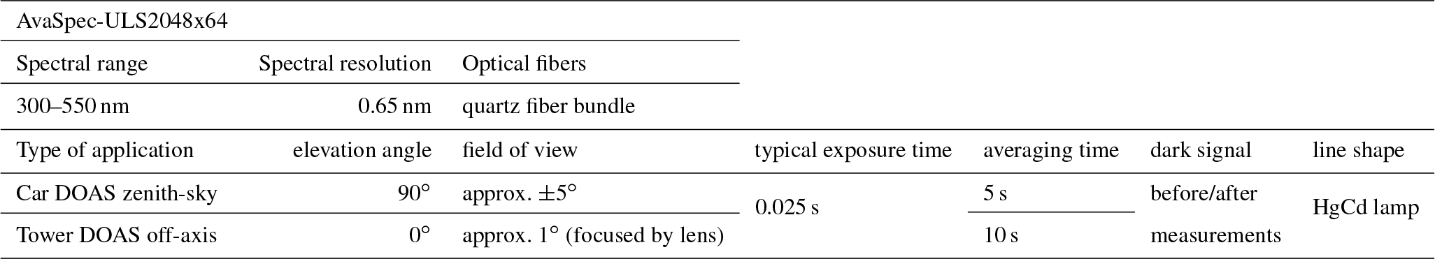
For the car DOAS zenith-sky and tower DOAS off-axis observations of tropospheric NO2 in Vienna, a DOAS system was used to measure scattered sunlight from directly overhead and from the horizon, respectively. A cardboard box was built to house a commercial Avantes miniature spectrometer (AvaSpec-ULS2048x64) and a notebook. The AvaSpec-ULS2048x64 is small in size ( mm), robust, and lightweight (855 g). The instrument performs spectral measurements between 290 and 550 nm at a spectral resolution of 0.65 nm (see Table 1). Both the spectrometer and notebook were supplied with electricity from the car battery and from the existing tower power circuit during the measurements.
2.2 Setup of the car DOAS zenith-sky measurements
An optical fiber was connected to the spectrometer and threaded through an aluminium bracket to the outside of the car, where it was fixed to a small aluminium plate by duct tape. In order to prevent direct sunlight from entering the optical fiber, a cylindrical plastic tube was used for shading the entrance. The field of view of the optical fiber was characterized in the laboratory to be about ±5∘. As the telescope was directed to the zenith, no large errors are expected for the retrieval of tropospheric vertical NO2 columns in this case as light path length is relatively insensitive to small deviations of the pointing from the zenith direction. For stability reasons, the bracket was clamped by the two door windows of the rear area. The geographical position of the car was recorded by a GPS receiver, which was connected to and powered by a USB port of the laptop computer.
The overall approach was to keep the measurement system simple. Therefore, only the zenith direction was implemented, which is insensitive to changes in pointing as from telescope misalignments or car movements. Pointing the instrument closer to the horizon increases the sensitivity to tropospheric NO2, but introduces an additional complication as pointing accuracy in a moving car becomes an issue. Experience also showed that in a city environment, a large fraction of the measurements at 22∘ or 30∘ elevation, for example, are affected by blocking from houses, trees, or other vehicles. As shown in previous studies (e.g., Wagner et al., 2010; Shaiganfar et al., 2011), the air mass factor for measurements at 22 and 30∘ depends on the relative azimuth between the telescope orientation and the sun, necessitating computation of the car heading from GPS data, which can be complex in typical city traffic situations. In summary, the choice was made to use a simple and robust method at the expense of reduced sensitivity.
A total of 20 identical car circuits around Vienna were performed on nine days in April, September, October, and November 2015 within the metropolitan area of Vienna (see Table 3). Each drive spanned about 110 km and lasted about 1.5 h. In order to minimize the effect of clouds and wind speed, measurements were performed in the morning rather than in the afternoon. After a successful test phase of the car DOAS zenith-sky measurements on 10 April 2015, more days were planned in fall of the same year, including working days and days on weekends as well as days with different wind conditions. Measurements between April and September, e.g., during the summer season, were unfortunately not possible due to other priorities and due the fact that the authors were not located in Vienna during that time.
Figure 1 illustrates an exemplary overview of a single car journey performed on 10 April 2015 between 05:27 and 06:59 UT. The starting point of each drive was within the municipality of Wolkersdorf im Weinviertel (48∘22′59′′ N, 16∘31′05′′ E), a small city located in Lower Austria, about 10 km north of Vienna and away from large sources of NOx. From there, the journey was planned to cover one of the busiest motorways in Austria, pass by known emission sources (e.g., power plants), and drive around one of the largest inland refineries in Europe, before heading back to the starting point on a different route. Also shown in Fig. 1 are the air quality monitoring stations that are used for comparison purposes (see Sect. 3.3) as well as the location of the Danube Tower, from which horizon measurements were performed (see the following Sect. 2.3).
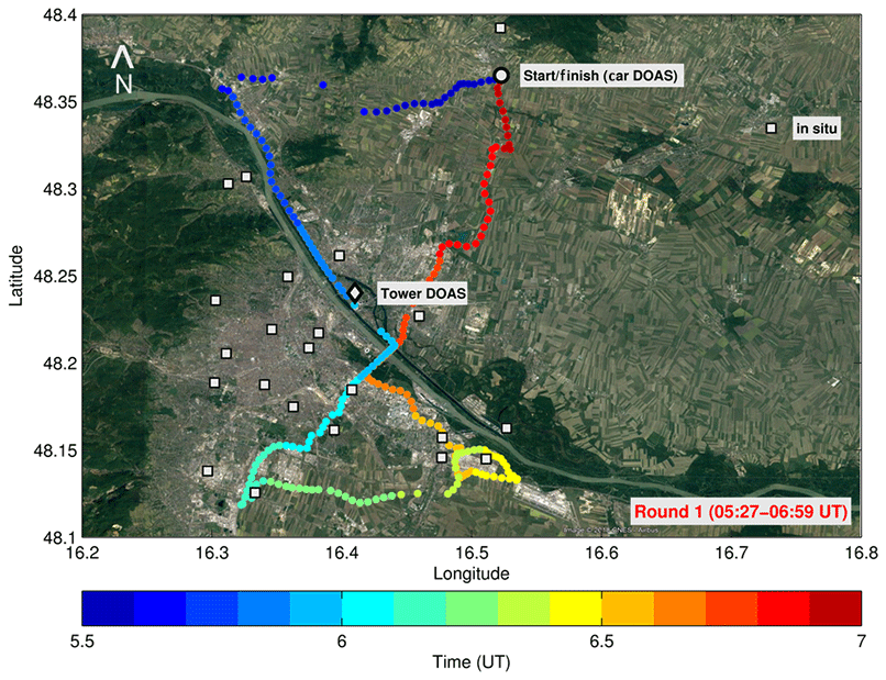
Figure 1Overview map with an example of a single car journey (color-coded dots) as performed on 10 April 2015 between 05:27 and 06:59 UT. The locations of the start and finish of the car journeys, Danube Tower, and in situ measurement stations are shown by a circle, diamond, and squares, respectively.
2.3 Setup of tower DOAS off-axis measurements
The same DOAS instrument was used for the measurements performed from the café at the Vienna Danube Tower (48∘14′25′′ N, 16∘24′36′′ E), which rotates at about 160 m above ground (https://www.donauturm.at, last access: 29 April 2019). Due to its geographical location (about 4.5 km to the northeast of the city center), it is possible to scan both urban and rural areas during a single counterclockwise 360∘ rotation (duration = 26.5 min). In contrast to the car DOAS zenith-sky measurements (see Sect. 2.2), the telescope was directed towards the horizon at an elevation angle of 0∘. An optical lens was placed in front of the light fiber entrance to reduce the field of view of the instrument to about 0.8∘. Both the lens and the entrance of the optical fiber were protected from direct sunlight by purpose-built cardboard. Because the scattered sunlight was passing through a thick glass window, no UV spectra could be recorded by the DOAS instrument from the rotating tower platform.
Tower DOAS off-axis observations were performed on five days in April and May 2016. More than thirty 360∘ scans of Vienna were recorded, each of them for an individual rotation of the café. For reasons of simplicity and accessibility, zenith-sky measurements were only taken afterwards from the open terrace, which is located a few meters below.
As the Vienna Danube Tower does not provide information on the exact orientation of the platform, and due to the fact that the signal of the GPS receiver was not accurate enough to reliably determine the position along the circle, the horizontal viewing angle was determined with the following approach: the Donau City Tower 1, the tallest skyscraper in Austria, which is located about 1 km from the Vienna Danube Tower, comes into field of view once every rotation and considerably reduces the signal (see Fig. 2). According to Google Earth, the position of the Vienna Danube Tower relative to this skyscraper is 167∘ (nearly south). Due to the constant rotation speed of the platform, which can be calculated from the DOAS observations, the horizontal viewing angle can be determined from the periodic sharp reduction in intensity.

Figure 2An example of a time series of the intensity of the spectrum as measured with the DOAS instrument from the rotating tower platform on 22 April 2016 between 12:25 and 14:35 UT. The sharp dips indicate a decrease in intensity due to pointing towards a skyscraper, which blocks the view of the instrument.
3.1 DOAS analysis
The spectral measurements as obtained during the individual car journeys and tower platform rotations are analyzed using the DOAS technique applying a nonlinear least-squares fitting algorithm. The spectral retrieval of NO2 differential slant column densities (DSCDs) is based on a fitting window between 425 and 490 nm, a polynomial degree of 5 (car DOAS zenith-sky) and 7 (tower DOAS off-axis), and a wavelength calibration using data from the solar atlas of Kurucz et al. (1984). These general settings have been commonly used in recent studies for the retrieval of NO2 DSCDs from ground-based DOAS-type measurements (e.g., Roscoe et al., 2010). High-resolution absorption cross sections of O3, NO2, O4, H2O, and a pseudo-cross section accounting for rotational Raman scattering as computed with QDOAS (Danckert et al., 2015) have been included in the two retrieval settings (see Table 2). The motivation for using a higher polynomial degree in the analysis of the horizon measurements is large broadband residuals found in the data. These residuals are attributed to the fact that the horizon measurements were taken through thick multilayer glass while the zenith-sky measurement was taken outdoors.
Table 2DOAS settings for the retrieval of NO2.
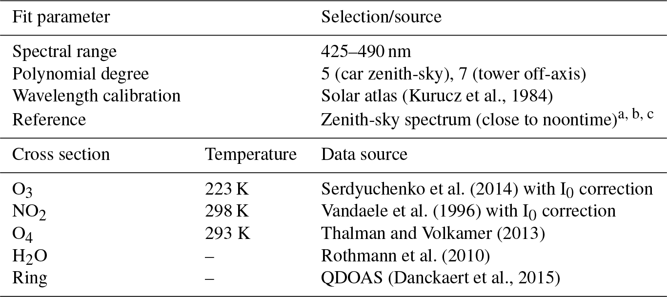
a Reference measurement for the retrieval of DSCDmeas on 10 April 2015 was taken on 10 April 2015 at 10:49 UT (48∘17′52.08′′ N, 16∘33′44.64′′ E). b Reference measurement for the retrieval of DSCDmeas on 27 and 28 September and 2 and 6 October 2015 was taken on 27 September 2015 at 10:17 UT (48∘21′52.75′′ N, 16∘31′20.24′′ E). c Reference measurement for the retrieval of DSCDmeas on 19, 23, and 27 October and 3 November 2015 was taken on 23 October 2015 at 10:14 UT (48∘21′53.85′′ N, 16∘31′22.48′′ E).
Table 3Summary of statistics of the individual car journeys including lap averages of wind speed, wind direction, temperature, pressure, number density of air, mixing height, in situ NO2 from selected air quality monitoring stations, and NO2 VCDtropo from car DOAS measurements. Converted averaged NO2 mixing ratios based on two different equations are also given. The correlation coefficients (R) obtained from the linear relationship between car DOAS and in situ NO2 are also shown (further details are given in the text).
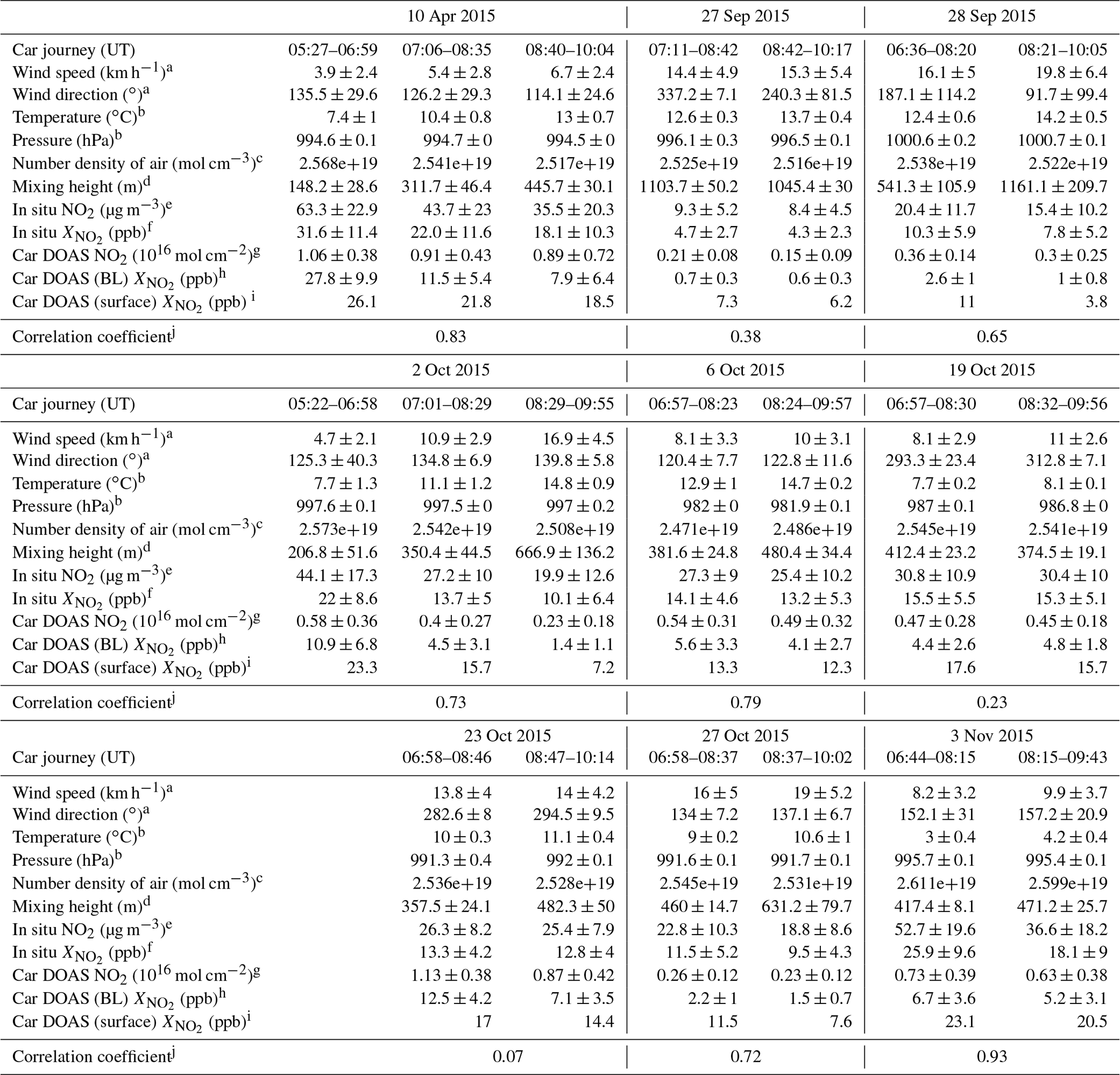
a Measurements from nine stations are provided by ZAMG. Values represent lap averages and standard deviations. b Measurements provided by the BOKU weather station. Values represent lap averages and standard deviations. c Calculations are based on the relationship between pressure and temperature measurements. Values represent lap averages. d Measurements provided by ZAMG. Values represent lap averages and standard deviations. e Measurements from 15 stations provided by UBA. Values represent lap averages and standard deviations. f Conversion of mass concentrations into mixing ratios is based on Eq. (5). Values represent lap averages and standard deviations. g Conversion of DSCDmeas into VCDtropo is based on Eq. (1). Values represent lap averages and standard deviations. h Conversion of VCDtropo into boundary layer mixing ratios is based on Eq. (3). Values represent lap averages and standard deviations. i Conversion of VCDtropo into surface mixing ratios is based on Eq. (4). j Values represent correlation coefficients between in situ NO2 (ppb) and car DOAS (BL) NO2 (ppb).
Exemplary car DOAS zenith-sky fit results, recorded on 10 April 2015 (SZA = 47.68∘) under elevated NO2 pollution (DSCD = 4.03×10¹⁶ mol cm−2), are shown in Fig. 3a, c. In some parts of the route, the zenith view of the instrument is obstructed by tunnels, bridges, or other objects. These measurements were identified using an intensity criterion and removed from the data set. However, some outliers having unrealistically high values of NO2 are still present in the data set, which strongly correlate with exceptional high chi-square values. Consequently, we only consider NO2 DSCDs with chi-square values < for further analysis. Noontime measurements of three selected days, taken in rural areas and close to air quality monitoring stations, are used as reference measurements (see Sect. 3.2.4 and Table 3).

Figure 3Exemplary fit results from the DOAS analysis in the 425–490 nm fitting window for a car DOAS spectrum (a, c), as measured on 10 April 2015 (SZA = 47.68∘, DSCD = 4.03×10¹⁶ mol cm−2) and averaged over intervals of 5 s as well as exemplary fit results for a tower DOAS spectrum (b, d), as measured on 29 April 2016 (SZA = 66.99∘, DSCD = 1.46×10¹⁷ mol cm−2) and averaged over intervals of 10 s.
Exemplary tower DOAS off-axis fit results obtained from a spectrum recorded on 29 April 2016 (SZA = 66.99∘) under elevated NO2 pollution (DSCD = 1.46×10¹⁷ mol cm−2) are shown in Fig. 3b, d. When comparing the two fit results, it becomes clear that the absorption by NO2 in the horizontal path is larger by a factor of 3.6 in this case. This is because most of the NO2 in urban environments is found in the boundary layer, close to the ground. In contrast, to the car DOAS zenith-sky measurements, no filtering was applied to the tower DOAS off-axis measurements.
The uncertainty of the retrieved unfiltered NO2 DSCDs was calculated from the fit. For car DOAS zenith-sky and tower DOAS off-axis measurements, this error is generally less than 0.75×10¹⁵ and 1.5×10¹⁵ mol cm−2, respectively
3.2 Car DOAS measurements of tropospheric NO2
3.2.1 Temporal resolution and computation of horizontal NO2 gradients
Typical exposure times for the car DOAS zenith-sky measurements were in the range of 0.00625 to 0.1 s. In most cases, however, the exposure time was 0.025 s. In order to obtain some information about the signal-to-noise ratio of the instrument and the horizontal gradients of NO2 present in the city, the temporal resolution of the car DOAS zenith-sky measurements was initially set to 0.05 s. The collected spectra were then averaged over intervals of 5 s (see Fig. 4), which corresponds to a traveled distance of about 100 m. An averaging interval of 5 s was also used by Constantin et al. (2013) for their mobile measurements.
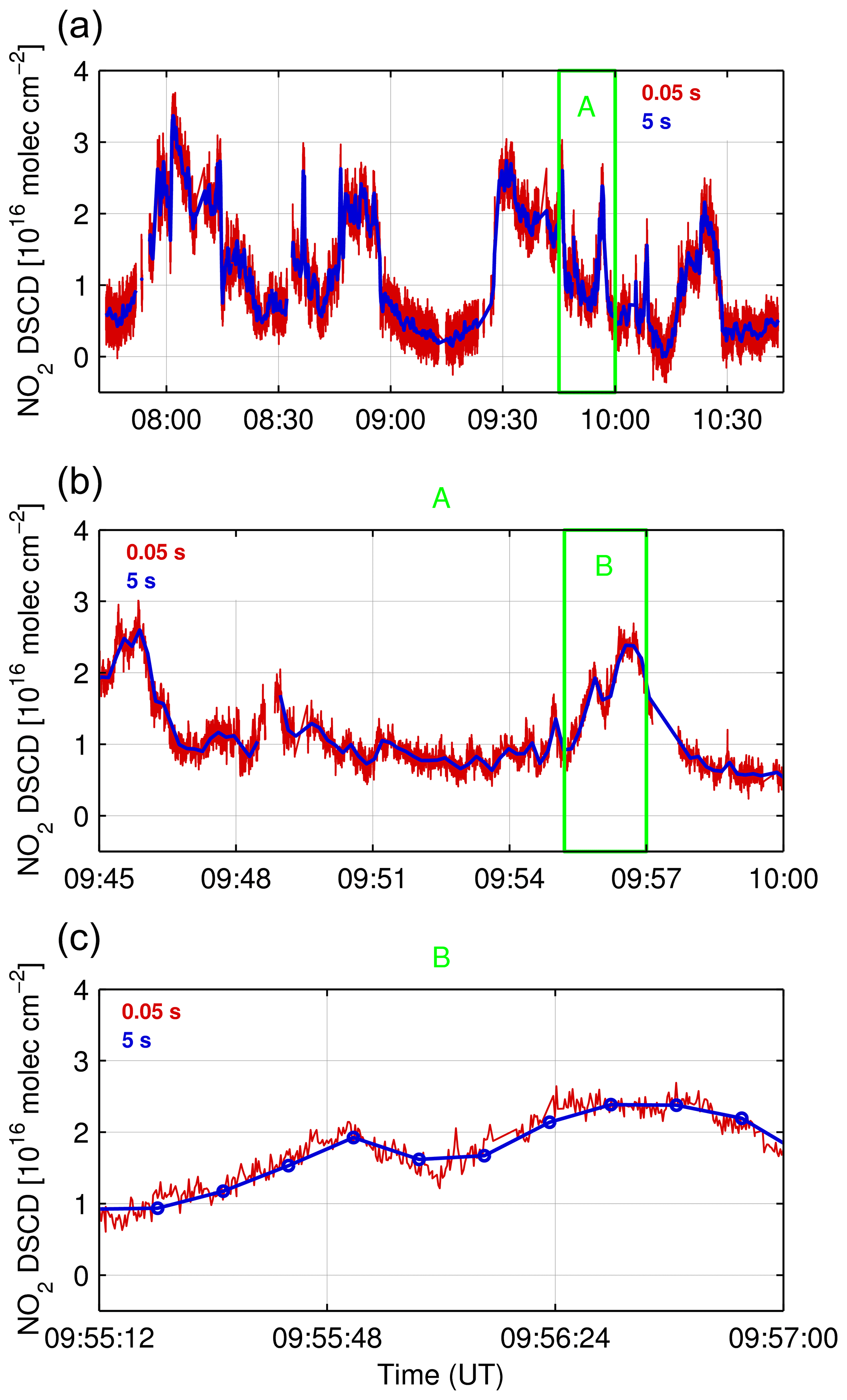
Figure 4Temporal resolution of NO2 DSCDs based on the car DOAS zenith-sky measurements performed on 3 November 2015. The red and blue lines show data at a resolution of 0.05 and 5 s, respectively. Panel (a) shows the NO2 DSCDs for the whole period of observations of that day, whereas (b) and (c) represent shorter time sections for clarity.
Figure 4a shows the temporal evolution of NO2 DSCDs on 3 November 2015. The red and blue lines represent the full resolution of 0.5 s and averaged values, respectively. While the full resolution is noisy (maximum deviation mol cm−2), the averaged values follow the general pattern of NO2 along the car route. For better clarity, Fig. 4b illustrates a shorter section of that day, indicated by the green box in Fig. 4a. The same is true for Fig. 4c, which represents a short section of Fig. 4b. Based on these results we argue that the selection of 5 s as an averaging interval appears to be optimal and a good compromise in our study, in spite of more information being found in the high-frequency data in some cases.
In addition to mapping the spatial distribution of NO2 in Vienna, it is also interesting to evaluate typical horizontal gradients within the city. The identification of such mean horizontal gradients of NO2 along the individual car routes is based on the following approach. Firstly, horizontal distances between the start and end points of individual car DOAS zenith-sky measurements at the full resolution of 0.05 s are calculated and summed. Secondly, NO2 DSCDs at the same time resolution are interpolated on 100 m bins as obtained from the first calculation step. Thirdly, absolute differences of NO2 DSCDs are derived for each pair of consecutive interpolated values within 5 km. In a final step, absolute differences are averaged along the car track in order to compute a mean horizontal gradient for each single car lap.
3.2.2 Stratospheric NO2 columns
The stratospheric correction in our study is based on stratospheric NO2 fields as simulated by the Bremen 3d chemistry transport model (B3dCTM) and scaled to satellite observations from the Global Monitoring Instrument 2 (GOME-2) over a selected region in the Pacific (180–140∘ W, 48–48.5∘ N) (Richter et al., 2011). This scaling is necessary as there is an offset between modeled and measured NO2 amounts.
Briefly, the B3dCTM, which evolved from SLIMCAT (Chipperfield, 1999), is a combined model approach based on the “Bremen transport model” (Sinnhuber at al., 2003a) and the chemistry code of the “Bremen two-dimensional model of the stratosphere and mesosphere” (Sinnhuber et al., 2003b; Winkler et al., 2008). It is driven by ECMWF ERA-Interim meteorological reanalysis fields (Dee et al., 2011).
Exemplary simulated stratospheric NO2 columns above Vienna as obtained from B3dCTM are shown in Fig. 5 for 19 October 2015. While stratospheric NO2 amounts sharply decrease in the morning due to photolysis of NO2, the observed increase in NO2 over the day is the result of dinitrogen pentoxide (N2O5) photolysis. The green rectangle indicates the start (06:57 UT) and end time (09:56 UT) of car DOAS zenith-sky measurements performed on 19 October 2015 (see also Table 3).
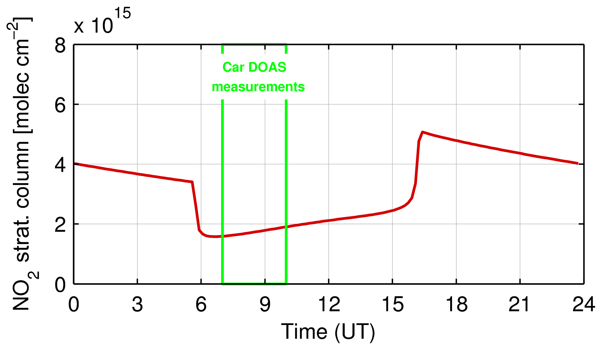
Figure 5Stratospheric NO2 above Vienna on 19 October 2014 (red line) as obtained from the Bremen 3d chemistry transport model (B3dCTM). The green rectangle indicates the time period of car DOAS measurements performed on that day.
In our study, the stratospheric model is only used for the diurnal cycle of the stratospheric NO2 column as the absolute value is scaled to GOME-2 satellite observations at the time of overpass. The uncertainty of the diurnal variation is large at twilight but small during the day as changes in stratospheric NO2 are small when compared to tropospheric NO2 columns in polluted regions, such as the urban area of Vienna. As a rough estimate, the uncertainty of the stratospheric correction is assumed to be less than 10 % or typically 1×10¹⁵ mol cm−2.
3.2.3 Simulation of tropospheric air mass factors
In order to apply appropriate tropospheric air mass factors for the conversion of DSCDmeas into VCDtropo (see Eq. 1) in our case study, different scenarios were simulated with the radiative transfer model SCIATRAN (Rozanov et al., 2014). The settings for these scenarios (see Table 4) are based on typical conditions over the urban area of Vienna during the time when car DOAS zenith-sky measurements were performed.
Table 4Parameter settings used for the simulation of tropospheric air mass factors with the radiative transfer model SCIATRAN.
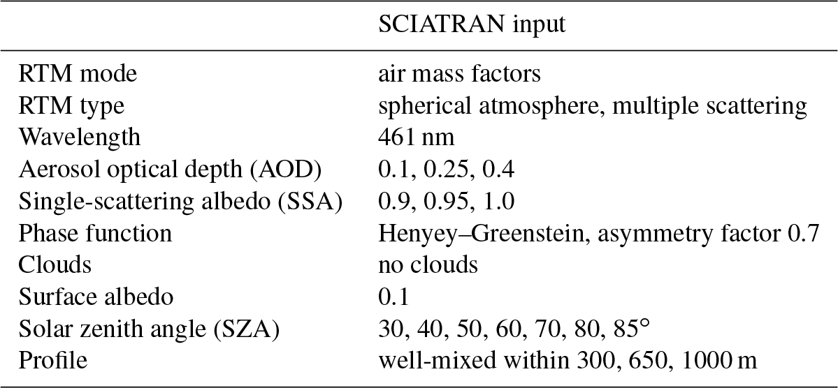
As a first step, extreme cases in terms of aerosol optical depth (AOD), single-scattering albedo (SSA), and mixing height (MH) were simulated. The results of the radiative transfer model (RTM) calculations are shown in Fig. 6, where scenario-based box air mass factors (AMFs) for an altitude range of up to 3 km are plotted for different SZAs. The results show that aerosols decrease the box AMF for small SZAs (30∘). With increasing SZA, however, the box AMF increases, in particular when approaching SZA = 80∘ and when aerosol loads are high. Within the aerosol layer, which is assumed to be well-mixed within the selected MH, the box AMF rises linearly with altitude. The results further suggest that SSA has only a small effect within the selected range of settings. Overall, the results of Fig. 6 suggest that aerosols strongly affect box AMFs as a function of SZA.
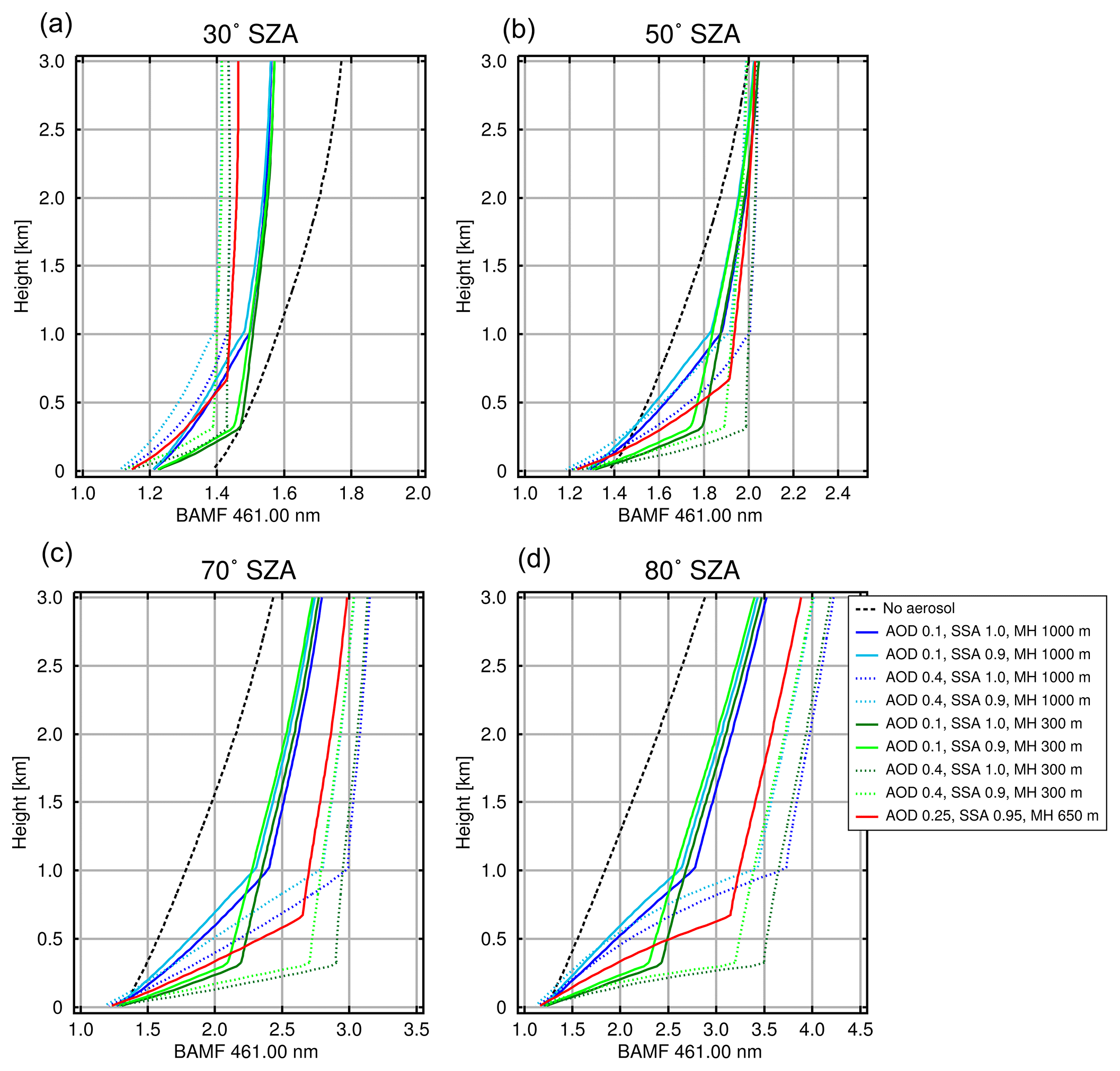
Figure 6Simulated scenario-based tropospheric box AMFs for SZA = 30∘ (a), SZA = 50∘ (b), SZA = 70∘ (c), and SZA = 80∘ (d). The red line shows the box AMF that is based on an intermediate scenario. Other scenarios are indicated by different colors and line styles.
Based on these results, we have decided to select an AMF used for the conversion of DSCDmeas into VCDtropo based on an intermediate scenario (AOD = 0.25, SSA = 0.95, and MH = 650 m), which according to our sensitivity study provides a good compromise. From the sensitivity study of AMF changes we conclude that all other scenarios are well within 20 % of these values selected for the intermediate scenario (see Fig. 7).
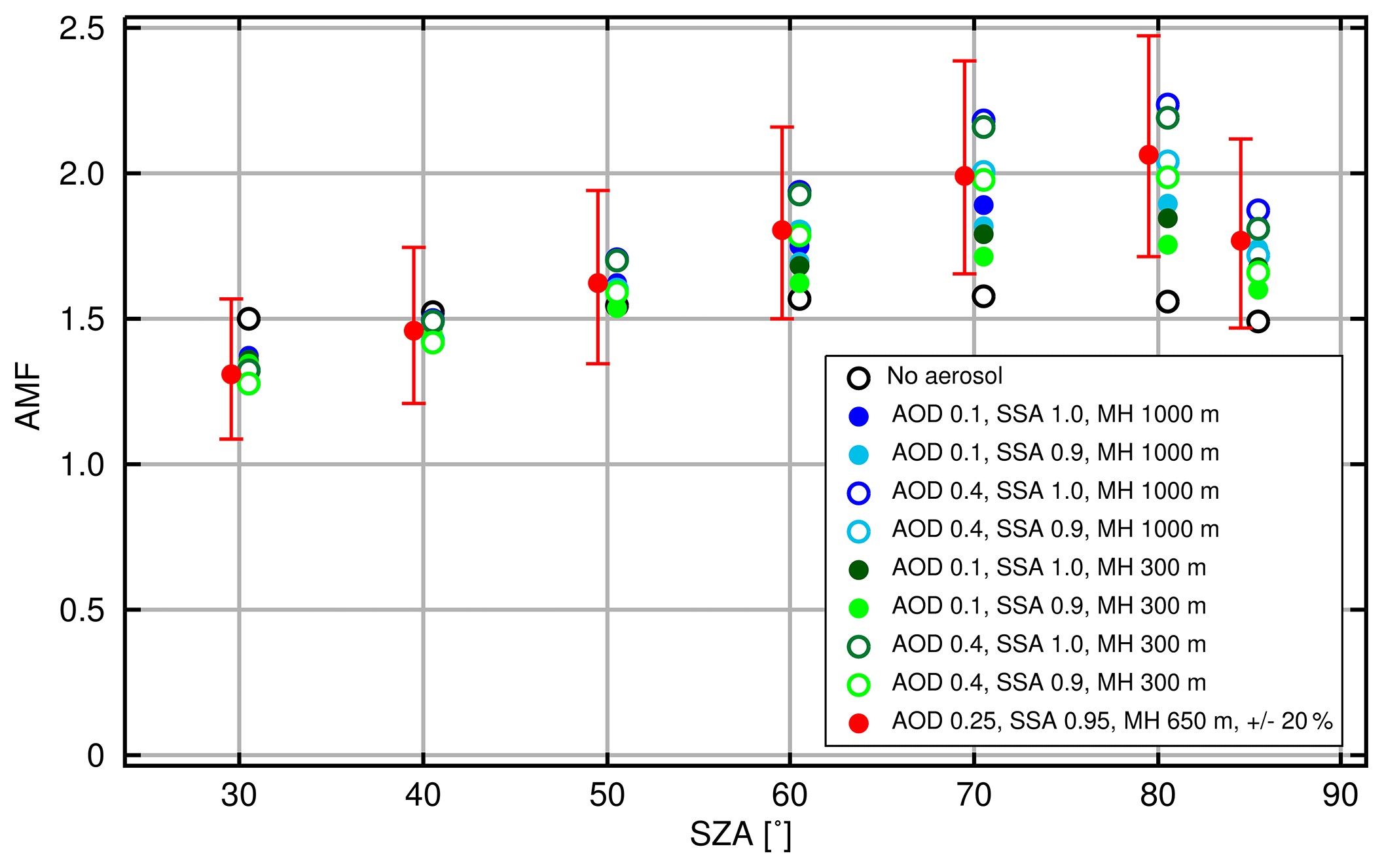
Figure 7Simulated scenario-based tropospheric AMFs as a function of SZA. The red dots represent the tropospheric AMFs that are used for the conversion of DSCDmeas into VCDtropo in this study (see Eq. 1); error bars indicate ±20 %. The other scenarios are depicted by circles and dots.
3.2.4 Conversion to tropospheric NO2 vertical column densities
The conversion of NO2 DSCDs obtained from car DOAS zenith-sky measurements into NO2 tropospheric vertical column densities (VCDtropo) is based on the approach by Wagner et al. (2010) and Constantin et al. (2013). The authors of the latter study have used a similar zenith-sky DOAS system on a car to derive tropospheric NO2 amounts in Romania. VCDtropo from car DOAS zenith-sky measurements is determined via the following equation:
where DSCDmeas is obtained from the car DOAS zenith-sky measurements by applying the DOAS analysis (see Sect. 3.1). SCDref is the slant column in the reference spectrum, which cannot be measured directly when applying the zenith-sky viewing mode only. Moreover, SCDref has both stratospheric and tropospheric amounts, which are estimated with different approaches in the literature (e.g., Wagner et al., 2010; Constantin et al., 2013; Tack et al., 2015). The residual amounts in SCDref (e.g., tropospheric NO2 amounts that remain after the subtraction of stratospheric NO2 amounts; see Eq. 1) in our study are calculated by applying an empirical relationship between VCDtropo and in situ NO2 mixing ratios as reported in Kramer et al. (2008). To be more specific, the estimation of residual amounts in SCDref is conducted for the time and location of the three selected reference measurements taken in rural areas outside the boundaries of Vienna and about 13 km (10 April 2015, 10:49 UT, SZA = 49.8∘, 48∘17′52.08′′ N and 16∘33′44.64′′ E) and 3 km (27 September, 10:17 UT, SZA = 50.33∘, 48∘21′52.75′′ N and 16∘31′20.24′′ E and 23 October, 10:14 UT, SZA = 59.96∘, 48∘21′53.85′′ N and 16∘31′22.48′′ E) away from the nearest air quality monitoring station. More details on data from air quality monitoring stations are given in the following Sect. 3.3. Stratospheric vertical column densities (VCDstrato) are derived from B3dCTM simulations and scaled to GOME-2 observations (see Sect. 3.2.2). Stratospheric air mass factors (AMFstrato) are calculated with the SCIATRAN radiative transfer model (Rozanov et al., 2014) and shown in Fig. 8 as a function of SZA. The simulation of tropospheric air mass factors (AMFtropo) is described in detail in Sect. 3.2.3.

Uncertainties in VCDtropo are introduced by uncertainties in the quantities used in Eq. (1). Assuming that the stratospheric AMF is well-known, the uncertainties of DSCDmeas, SCDref, SCDstrato, and AMFtropo need to be considered. For a typical situation, an overall uncertainty of 25 % is found, dominated by the assumed 20 % uncertainty of the AMF (see Sect. 3.2.3). For situations approaching twilight, the absolute uncertainty of the stratospheric correction increases, and the relative uncertainty of the slant column can become the dominating error source. If the background measurement SCDref cannot be taken in a clean region, then the absolute uncertainty on this quantity can become large and important for the overall uncertainty (see Wagner et al., 2010). As our car DOAS zenith-sky measurements were performed after morning twilight and because SCDref was taken outside the city of Vienna in rural areas, an overall uncertainty of 25 % seems to be realistic for our study.
3.3 In situ measurements of NO2
For the estimation of residual amounts in SCDref as well as for the comparison of NO2 VCDtropo obtained from car DOAS zenith-sky (see Sect. 4.4) and NO2 mixing ratios from tower DOAS off-axis measurements (see Sect. 4.5) with in situ NO2 concentrations, data from 23 air quality monitoring stations in and around Vienna, provided by the Environment Agency Austria, UBA (Umweltbundesamt), are used (see Fig. 1). For the detection of NO2 concentrations, Horiba APNA-370 and API M200E (NOx) instruments are currently used at most of these stations. In addition, TEI 42i and Horiba APNA-360E instruments are operated at individual stations (Spangl, 2017). The combined measurement uncertainty for these instruments is about 10 % (W. Spangl, personal communication, 2018).
Residual amounts in SCDref are calculated by converting simultaneous in situ NO2 measurements from the air quality monitoring stations in Gänserndorf (10 April 2015) and Wolkersdorf (27 September and 23 October 2015) into VCDtropo applying the empirical relationship between concurrent MAX-DOAS and urban background in situ measurements (Kramer et al., 2008):
where y is the tropospheric NO2 VCD (residual amounts in SCDref in our study) in units of 1016 mol cm−2 and x denotes the in situ NO2 mixing ratios in units of parts per billion. The conversion of in situ NO2 concentrations (µg m−3) into in situ NO2 mixing ratios (ppb) in our study is described in Sect. 3.5.
The residual amounts in SCDref as determined with Eq. (2) are estimated at 1.3×10¹⁵, 1.1×10¹⁵, and 2.2×10¹⁵ mol cm−2 on 10 April, 27 September, and 23 October, respectively. We note that the extrapolation of the empirical relationship to our measurements is critical in a sense that meteorological conditions and emissions are not the same in Leicester and Vienna. Due to the fact that SCDref measurements were taken outside of Vienna in our study, with in situ measurements of NO2 being in the range of 2.5 to 6 ppb on those three days and indicating rather low residual amounts, the error is assumed to be likewise low in this case.
For the comparison of car DOAS zenith-sky and in situ NO2 observations, we have selected half-hour averages of NO2 concentrations from seven stations in Lower Austria and eight stations in Vienna that are within 5 km of the car route (see Fig. 1). The selection of appropriate in situ NO2 observations for the comparison with tower DOAS off-axis measurements is described in Sect. 4.5. For both cases, half-hour averages of NO2 concentrations are converted into mixing ratios (see Sect. 3.5).
3.4 Mixing height from ceilometer observations
The conversion of VCDtropo into mixing ratios as described in the following Sect. 3.5 requires, in addition to meteorological measurements of pressure and temperature, information on the planetary boundary layer depth (also known as mixing height). The Austrian official weather service, ZAMG (Zentralanstalt für Meteorologie und Geodynamik), performs operational aerosol-layer height measurements with a Vaisala CL51 ceilometer at the Hohe Warte site in the northwest of Vienna (48∘14′55′′ N, 16∘21′23′′ E). Mixing-height (MH) time series are obtained from these measurements by removing unrealistic nocturnal aerosol-layer height values, avoiding outliers, filling data gaps by linear interpolation, and smoothing (Lotteraner and Piringer, 2016). Mixing-height data at a temporal resolution of 5 min were provided by ZAMG for those days when car DOAS zenith-sky measurements were carried out.
3.5 Comparison of NO2 mixing ratios obtained from car DOAS zenith-sky and in situ measurements
The comparison between the two independent NO2 observations (car DOAS zenith-sky versus in situ) is based on gridding the data of both measurement techniques onto a spatial resolution. For a better comparison, NO2 VCDtropo as obtained from car DOAS zenith-sky measurements as well as in situ NO2 concentrations are converted into mixing ratios. The former conversion is based on recommendations made in Knepp et al. (2013). The authors of that study have converted Pandora tropospheric NO2 values into mixing ratio values by applying a planetary boundary layer (PBL) height correction factor. Although this approach assumes a constant mixing ratio in the PBL, which is not necessarily correct in an urban environment, it accounts for the variability in MH throughout the day. We follow their approach and estimate boundary layer mixing ratios of NO2 () via the following equation:
where MH is the mixing height (PBL in their study) and na denotes the number density of air (N in their study). Here, we use lap averages for MH as calculated from the data in 5 min resolution provided by ZAMG (see Sect. 3.4). The standard deviation of these lap averages generally ranges between 10 and 50 m but can be as high as 200 m when wind speeds are high (see Table 3). The number density of air, which is related to the atmospheric pressure by the ideal gas law, is also averaged over the individual car laps. Meteorological measurements of pressure (p) and temperature (T) used for the calculation of na are provided by the BOKU (Universität für Bodenkultur) weather station, located in the northwest of Vienna (48∘14′16.45′′ N, 16∘19′54′′ E). We note that the weather station is located about 100 m higher than the altitude level of the car route. Thus, pressure might be slightly lower when compared to the pressure level 100 m below. Conversely, the weather station is also located outside of the city center, at the foot of the hills in the northwest and in a less densely populated residential area with many green areas, resulting in slightly cooler temperatures than expected for other places along the car route. Following this reasoning, it becomes clear that the altitude difference might cancel in the calculation of na (see Eq. 3) and also in the following Eq. (5).
Recently, Dieudonné et al. (2013) highlighted the fact that large vertical gradients of NO2 concentrations exist over urban areas. The authors of that study suggest that the averaged concentration within the PBL is only about 25 % of NO2 surface concentration measurements when NO2 profiles from chemistry transport models are assumed for the PBL. Following this reasoning, car DOAS (BL) as estimated via Eq. (3) does not represent NO2 near-surface mixing ratios sufficiently well and a comparison with NO2 as obtained from air quality monitoring stations and converted into in situ (see Eq. 5) is not yet reasonable. Consequently, an empirical approach for estimating near-surface NO2 mixing ratios from the car DOAS zenith-sky measurements is introduced in our study, in addition to car DOAS (BL) .
In order to achieve optimal agreement between car DOAS zenith-sky measurements and in situ observations in our study, we include four parameters that are expected to affect the vertical NO2 gradients and conduct a linear regression analysis as follows:
where Y is the expected value of the dependent variable in situ (see Eq. 5) and X1, X2, X3, and X4 are the independent variables VCDtropo NO2, MH, wind speed, and na, respectively (see Table 3).
The conversion of in situ NO2 concentrations (cm) into mixing ratios is based on the equation
where Mi is the molecular weight of NO2 and R denotes the universal gas constant. As for the calculation of na, p and T measurements at a 10 min resolution are taken from the BOKU weather station and averaged for the individual car laps.
All NO2 mixing ratio values within individual grid cells are averaged and then compared with each other.
3.6 Meteorological measurements of wind direction and wind speed
Most of the emission sources other than traffic are located in the southeast of Vienna. The wind blew exactly from this direction on several days when car DOAS zenith-sky measurements were carried out. In addition, the car journey was planned to include the motorway along the Danube River, spanning a distance of about 20 km from the northwest (48∘21′25′′ N, 16∘18′25′′ E) to southeast (48∘12′32′′ N, 16∘26′24′′ E). These are prerequisites for the optimal analysis of the evolution of NO2 in space and time, in particular on days when wind was blowing from either the northwest (NW) or southeast (SE). As there are no large sources of NOx located in the NW, we rather focus on days when wind was blowing from the SE.
Data on wind direction and wind speed are provided by ZAMG. We have selected such data from four stations in Lower Austria and five stations in Vienna that are in close proximity to the car route (see Table 5). The temporal resolution of these measurements is 10 min. Instead of attempting to map the wind direction to the car route in time, we have averaged these measurements over the period between the start and end time of each car journey and calculated the standard deviation (see Table 3).
Table 5Overview of selected meteorological stations, operated by the Austrian official weather service.

3.7 Tower DOAS measurements of tropospheric NO2
3.7.1 Temporal resolution and normalization of NO2 DSCDs with O4
Compared to the car DOAS zenith-sky measurements, the temporal resolution of spectral measurements performed on the rotating tower platform is higher (0.025 s). This is because of the relatively fast rotation speed resulting in a full 360∘ rotation within only 26.5 min. Again, these temporally highly resolved spectral measurements are averaged, but this time over 10 s. After the averaging procedure, roughly 150 measurements remain for a single 360∘ rotation. These observations are then interpolated on 3.6∘ segments, resulting in 100 measurements for one single rotation.
One of the main drawbacks of the measurements is that only one reference measurement was taken after the measurements. This was because no zenith-sky measurement was possible from within the café, and no second DOAS system was available during that time for parallel measurements from the surface. Therefore, a fixed zenith spectrum has to be used instead of a sequential one, resulting in an increasing effect of a changing tropospheric light path (due to geometry, aerosols, phase function, etc.) with increasing time difference between the off-axis and fixed zenith spectra. One way of overcoming this problem is to normalize NO2 DSCDs with O4 DSCDs, which is done for all measurements taken.
3.7.2 Computation of path-averaged NO2 mixing ratios
A modified geometrical approach (MGA) for estimating long-path averaged mixing ratios of trace gases (e.g., NO2) from MAX-DOAS measurements at high-altitude sites was proposed in a recent study by Gomez et al. (2014). The method assumes a single-scattering geometry and a scattering point altitude close to that of the instrument. Under these assumptions, the slant paths of the zenith () and horizontal () measurements are identical up to the scattering point and thus cancel in the DSCD when using a zenith-sky background spectrum close in time. For measurements performed at higher altitudes, the MGA can be applied without any correction factors, in particular when the instrument is located well above the PBL and aerosol amounts are negligibly low (Schreier et al., 2016). For MAX-DOAS measurements carried out close to the ground level, however, the MGA is limited because of a substantial aerosol load and correction factors are needed (Sinnreich et al., 2013). Nevertheless, Seyler et al. (2017) have recently successfully utilized the MGA for MAX-DOAS measurements of shipping emissions in the German Bight – without the use of correction factors. According to their findings, typical lengths of horizontal light paths in the visible spectral range are in the range of 12.9±4.5 km on average and can reach up to 15 km on days with optimal visibility. It should be noted, however, that the non-consideration of correction factors in polluted environments such as the German Bight will lead to a systematic overestimation of horizontal path lengths, depending on the aerosol load.
In our study, where the rotating tower platform is also located close to the ground level, we overcome this problem by making the following assumptions. Firstly, we assume that the signal for horizontal measurements (α=0∘) is dominated by the horizontal part of the light path after the last scattering event. Secondly, a hill named Kahlenberg (484 m a.s.l.) located in the northwest of the Vienna Danube Tower (305∘) comes into the field of view once every rotation. We assume that the hill limits the horizontal optical path length (hOPL) under clear-sky conditions and use the distance between the summit of the hill and the Vienna Danube Tower (6.95 km) as the normalization value. The conversion of DSCD O4 at α=0∘ is realized by relating this distance with the obtained DSCD O4 value at 305∘ and applying the resulting relationship to all other DSCD O4 values observed during the same tower platform rotation. We assume that the change in DSCD NO2 in the vertical (α=90∘) can be neglected for (polluted) urban environments over the course of one tower rotation. The latter assumption has to be made because no sequential zenith-sky spectra are available. Therefore, path-averaged NO2 mixing ratios are only estimated and presented for the last tower rotations of the individual days, having the zenith-sky reference spectrum as close as possible in time.
When taking all these assumptions into consideration, path-averaged mixing ratios of NO2 can be estimated with the following equation:
For the calculation of na, rotation averages of pressure and temperature as provided by the BOKU weather station are used (see Sect. 3.5).
4.1 Horizontal gradients of NO2 DSCDs
As the car DOAS zenith-sky measurements provide, in addition to the temporal distribution, the horizontal variation in NO2, the method described in Sect. 3.2.1 is applied to the car DOAS zenith-sky observations to determine horizontal gradients of NO2.
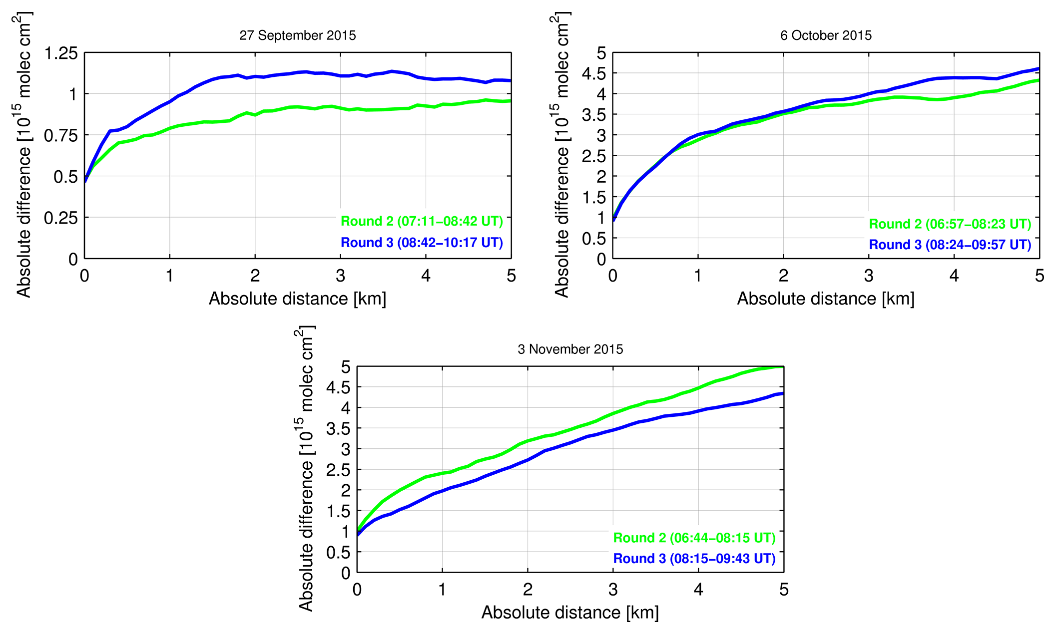
Figure 9Mean absolute difference in NO2 DSCDs as a function of the absolute distance (see Sect. 3.2.1) for car DOAS zenith-sky measurements performed on three selected days with different wind conditions and NO2 levels.
In Fig. 9, typical examples of such horizontal gradients are presented for 27 September (Sunday), 6 October (Tuesday), and 3 November (Tuesday) 2015 – three days with different wind conditions, temperature levels, and tropospheric NO2 amounts (see Table 3). In general, an increase in absolute NO2 differences with increasing distance from the individual starting points is found. While absolute NO2 differences sharply increase within the first one or two kilometers for most of the journeys, the increase significantly weakens during the remaining kilometers. During the first kilometer, absolute NO2 differences increase by a factor of 1.5 to 4, depending on the overall NO2 level on the investigated days. While the absolute NO2 differences rise by a factor of about 2 within the first two kilometers on 27 September, an increase by a factor of almost 4 is found for the same distance on the more polluted 6 October 2015.
The results imply that the magnitude of absolute NO2 differences is linked to the magnitude of tropospheric NO2 amounts observed. Conversely, it is difficult to detect the factors affecting the shape of the derived curves. Interestingly, we found only small differences in the shape and magnitude of horizontal NO2 gradients when comparing individual car journeys of single days with each other. Only for days with significant changes in wind direction (e.g., 27 September 2015) are the differences in magnitude obvious, when the single laps are compared with each other. While the curves of 10 April (not shown) and 6 October are similar in shape, the typical sharp increase within the first two kilometers is not observed for 3 November, although average values of wind speed, wind direction, and mixing height were similar on those days (see Table 3). It is not clear why the shape of NO2 as a function of distance observed on 3 November differs from those found on the other two days. One reason could be variations in photochemistry and/or emissions and/or dilution of NOx. It is interesting to note that 3 November 2015 was clearly the coldest day with temperatures below 5 ∘C (see Table 3). As a result, we argue that the characteristic horizontal NO2 scale of the observed NO2 fields in Vienna is on the order of 1 to 2 km.
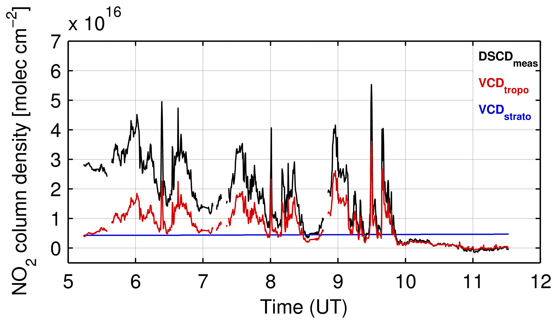
Figure 10Time series of NO2 DSCDmeas (black), VCDtropo (red), and VCDstrato (blue) obtained from car DOAS zenith-sky spectra recorded on 10 April 2015.
4.2 Spatiotemporal patterns of tropospheric NO2 obtained from car DOAS zenith-sky measurements
Figure 10 shows typical car DOAS zenith-sky measurements of NO2 performed on 10 April 2015. The black and red curves represent DSCDmeas and VCDtropo, respectively. The stratospheric NO2 amounts as simulated by B3dCTM and scaled to GOME-2 observations (see Sect. 3.2.2) are illustrated by the blue line. Clearly, stratospheric NO2 is relatively low in this case of increased tropospheric NO2 levels when compared to VCDtropo. The relatively small diurnal increase in NO2 in the stratosphere can hardly be seen for the 6 h period. There are individual peaks in NO2 throughout the morning of 10 April 2015. While the longer lasting NO2 peaks are probably connected to pollution from traffic, sharp peaks rather indicate some outflow of NO2 from the refinery and/or other local static emission sources. The magnitude of observed NO2 VCDtropo is in good agreement with measurements performed around the German cities Mannheim and Ludwigshafen as well as in the Romanian city Braila (Ibrahim et al., 2010; Dragomir et al., 2015). As expected, significantly higher values of NO2 VCDtropo were observed by Wang et al. (2012) in the central urban area of Shanghai, China.
In the following, the small-scale transport of NO2 is evaluated along the Donauufer motorway (A22) in more detail. The A22 motorway, which is identifiable in Fig. 1 by azure and turquoise dots (NW to SE), is one of the busiest roads in Vienna, in particular in the southeastern area, where many commuters take the Südosttangente motorway (A23) at the motorway junction Kaisermühlen. The A23 is another busy road in Austria having about 160 000 passenger cars driving on it every day on average (https://www.vcoe.at, last access: 29 April 2019). As a consequence, NO2 levels are expected to be significantly increased in this area, in particular during the morning and evening rush hours.
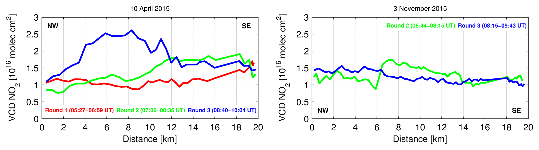
Figure 11Temporal evolution of tropospheric NO2 for the car DOAS zenith-sky measurements as performed on 10 April and 3 November 2015. The red, green, and blue curves represent NO2 VCDtropo as obtained along the A22 during the first, second, and third journeys, respectively.
The NO2 variation along the A22 motorway is shown in Fig. 11 for Friday, 10 April and Friday, 3 November 2015 as a function of cumulative distance, where the starting and end points are in the NW and SE of the A22 motorway. The red, blue, and green curves represent NO2 VCDtropo during the first, second, and third drives, respectively. In order to not confuse the reader, the first and second rounds of days with measurements taken only during two rounds are here referred to as rounds two and three, starting approximately at 07:00 and 08:30 UT, respectively (see Table 3). While wind was blowing from the SE on both days, averages of wind speed were slightly higher on 3 November.
On 10 April, the highest NO2 VCDtropo is observed in the SE rather than in the NW during the first drive. This seems reasonable as the traffic volume is generally largest in this area, in particular during the morning rush hour, which is captured by the first drive of that day. NO2 loads then move to the NW of the A22 motorway because air masses are transported from the SE. A clear shift of NO2 pollution from the SE to the NW is observed on 10 April 2015. The highest NO2 VCDtropo values during the first (> 1.5×10¹⁶ mol cm−2), second (< 2.0×10¹⁶ mol cm−2), and third drives (> 2.5×10¹⁶ mol cm−2) are located around 19.5, 18.5, and 8.5 km away from the starting point in the NW, respectively. Interestingly, the observed NO2 peak during the last drive is very pronounced. We attribute this to the NO2 formation via the chemical reaction of NO with ozone towards noontime. The topography in this area could also be responsible for these high NO2 levels. There are two hills east (Bisamberg, 358 m a.s.l.) and west (Kahlenberg, 484 m a.s.l.) of the Danube River. As a consequence, the pollution load could be channeled between the two hills, leading to a localized increase in NO2 amounts in this area.
The distance of NO2 transport appears larger between the second and third drives when compared with distances of NO2 transport between the first and second journeys. This might be related to the increase in average wind speed throughout the morning (see Table 3). Overall, the distance of NO2 transport on 10 April 2015 is in good agreement with average wind speed. Due to higher wind speeds on 3 November 2015, the expected peaks of NO2 in the NW during the third journey cannot be seen anymore. This might be related to the high averaged wind speeds during the second and third drives (between 8 and 10 km h−1) and thus a distance of transport exceeding the area of evaluation. Conversely, a clear shift of elevated NO2 amounts into the NW is also observed for the second round on 3 November 2015. It is interesting to note that the horizontal extent of elevated NO2 amounts during the third round of 10 April and during the second round of 3 November 2015 spans about 8 km in both cases – under similar wind speeds. We argue that this is a characteristic horizontal extent of a NO2 plume resulting from morning rush-hour traffic in Vienna under calm southeasterly winds.
4.3 Spatiotemporal patterns of tropospheric NO2 obtained from tower DOAS off-axis measurements
The spatial and temporal variation in tropospheric NO2 amounts is also evaluated by analyzing the tower DOAS off-axis measurements. In order to correct light path lengths in the troposphere, NO2 DSCDs are normalized with O4 DSCDs. When looking at the time series of intensity (see Fig. 2), NO2, and O4 (Fig. 12), it becomes apparent that these parameters show variations as a function of azimuth angle. This variation is repeated with each further tower platform rotation. Although some similarity is found between DSCD NO2 and O4, the highest and lowest amounts of both trace gases are somehow shifted on the x axis. Some similarity between DSCD O4 and NO2, which is observed on all five days (not shown), is attributed to changes in the light path. Interestingly, the normalization with O4 slightly changes the azimuthal position of the pollution peaks towards the city center.
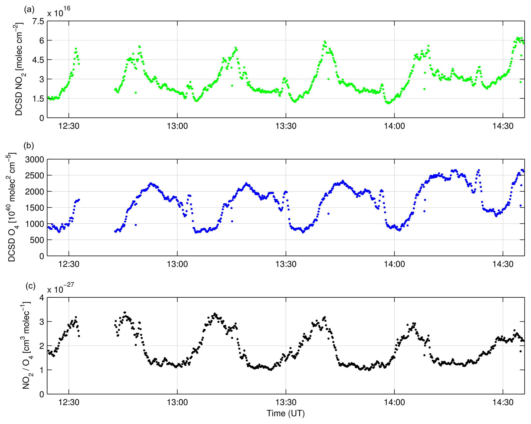
Figure 12Time series of NO2 (a) and O4 (b) DSCDs as obtained from the tower DOAS off-axis measurements performed on 22 April 2016. The ratio of NO2∕O4 is shown in (c).

Figure 13Spatial and temporal variability of the NO2∕O4 ratio (here, the radius is determined by DSCD O4 values) on 10 May 2016 between 05:57 and 09:56 UT observed by tower DOAS off-axis measurements. The position of the Vienna Danube Tower (DT) is highlighted in the center of the geographical map. The white asterisk represents the summit of Kahlenberg (484 m a.s.l.), which is used for the estimation of horizontal optical path lengths.
The geographical distribution of DSCD NO2 and O4 is shown in Fig. 13 for 10 May 2016, when tower DOAS off-axis measurements during nine platform rotations were collected. The values plotted on the map are mean NO2∕O4 values and the radius is the O4 column. On that day, wind was mainly blowing from easterly to southeasterly directions. As a result, the highest NO2∕O4 ratios are observed towards the city center.
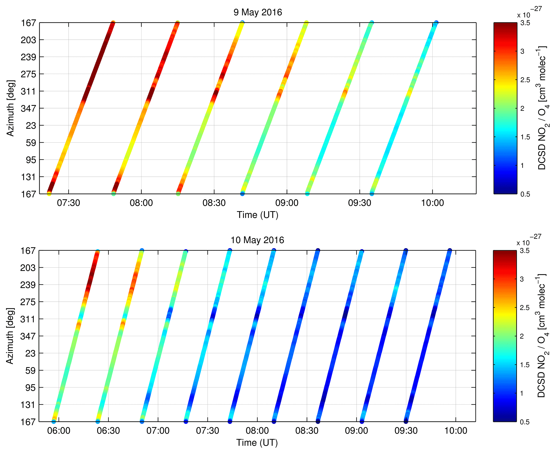
Figure 14Spatial and temporal variability of DSCD NO2∕O4 obtained from tower DOAS off-axis measurements performed on 9 and 10 May 2016.
The spatial and temporal variability of DSCD NO2∕O4 as obtained from tower DOAS off-axis measurements is shown in Fig. 14 for 9 and 10 May 2016. As already identified from the analysis of the car DOAS zenith-sky measurements, the highest tropospheric NO2 over Vienna is found in the early morning – a consequence of both a lower (nocturnal) mixing height and emissions of NOx from morning rush-hour traffic. The highest NO2 amounts on both days are generally observed over the city center of Vienna, which is located to the southwest of the Vienna Danube Tower. A closer look suggests that DSCD NO2∕O4 is about a factor of 2 larger on 9 May than on 10 May. While wind was constantly blowing from the SE on both days, the explanation for this is most likely the higher wind speeds on 10 May.
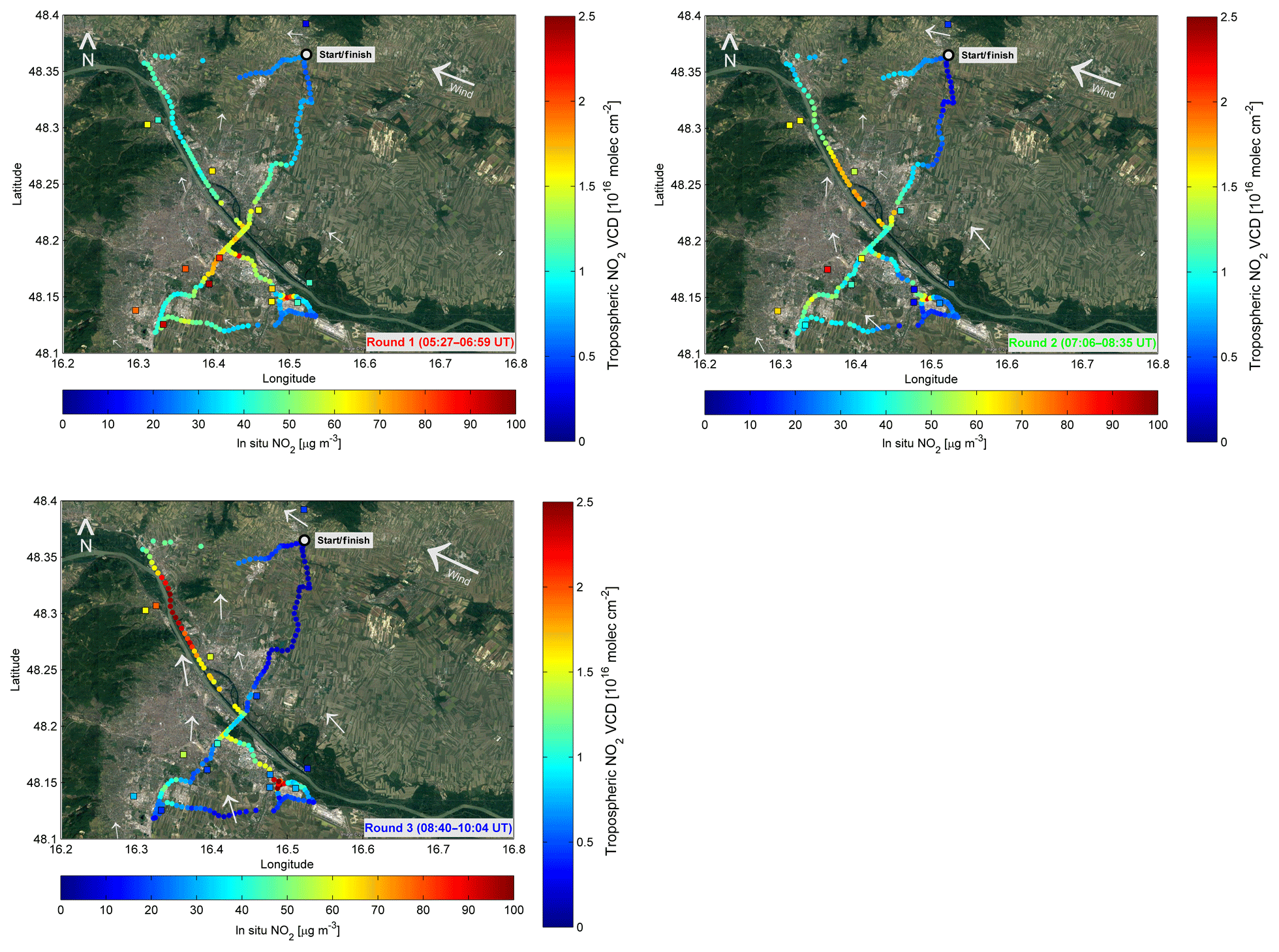
Figure 15Spatial and temporal evolution of NO2 on 10 April 2015 in Vienna as measured by the car DOAS zenith-sky (dots) and in situ surface measurements (squares). Wind direction and wind speed obtained from local weather stations are indicated by white arrows. The size of the arrows is weighted by the corresponding averaged wind speed (2 m above ground) obtained from the individual weather stations. Averaged wind speeds over the course of the car DOAS zenith-sky measurements taken on this day ranged between 2.28 and 12.81 km h−1.
4.4 Comparison of NO2 from car DOAS zenith-sky measurements with in situ NO2
The spatial and temporal evolution of NO2 on 10 April 2015 in Vienna as observed by car DOAS zenith-sky (dots) and in situ measurements (squares) is shown in Fig. 15. Wind direction and wind speed obtained from local weather stations are indicated by white arrows. The geographical maps illustrate the spatial distribution of tropospheric NO2 during the three performed journeys on that day. As already highlighted in Sect. 4.2, a clear change in the amount of NO2 throughout the morning is observed along the motorway A22. A large proportion of observed NO2 amount is produced from traffic emissions of NOx during the morning rush-hour traffic, in particular in the area southeast of the city center. During the time period of about 4.5 h between the starting and end points of the measurements performed on that day, NO2 is transported over a distance between 10 and 15 km. Another hot spot of increased NO2 levels is observed close to an oil refinery in the SE. The outflow of the refinery is in good agreement with wind direction on that day. As already mentioned in Sect. 4.2, such peaks of NO2 amounts as a result of local static emission sources are sharper than those originating from typical rush-hour traffic. There is a clear decrease in tropospheric NO2 throughout the morning (see also Table 3), most likely as a consequence of dilution and/or the reaction of NO2 with the hydroxyl radical (OH), which is the largest NOx sink during daytime.
Overall, averages of tropospheric NO2 observations were highest on 10 April and 3 November 2015. We attribute this behavior to the comparatively low wind speeds, and consequent low dilution.
As outlined in Sect. 3.5, the correlation of the two data sets (car DOAS zenith-sky versus in situ) uses data converted into NO2 mixing ratios, which are values gridded onto cells. The correlation is performed for each single day when car DOAS zenith-sky measurements were carried out. The scatter plots including statistics about slope, intercept, and correlation coefficient are illustrated in Fig. 16. Each of the diamonds represents a grid box average of from car DOAS zenith-sky measurements as a function of averaged from in situ monitors. The correlation coefficient on 10 April 2015, for example, is 0.83, suggesting a close linear relationship of the two independent NO2 measurements on that day (see also Table 3). The apparent negative offset implies that in situ is higher than estimated via Eq. (3). While this is the case for the grid box averages calculated from measurements taken during the second and third journeys of that day, values from car DOAS zenith-sky observations seem to be overestimated during the first journey. A similar result with slightly lower values for R and slope is observed on 2 October, the second day, when early morning measurements were performed and when wind was also blowing from the southeast. The reason for the better agreement in the early morning (e.g., during the first car journey) could be the lower MH and lower wind speed, resulting in a better vertical mixing within the shallow boundary layer. The increase in both MH and wind speed throughout the morning might counteract a vertical mixing of NO2 loads.
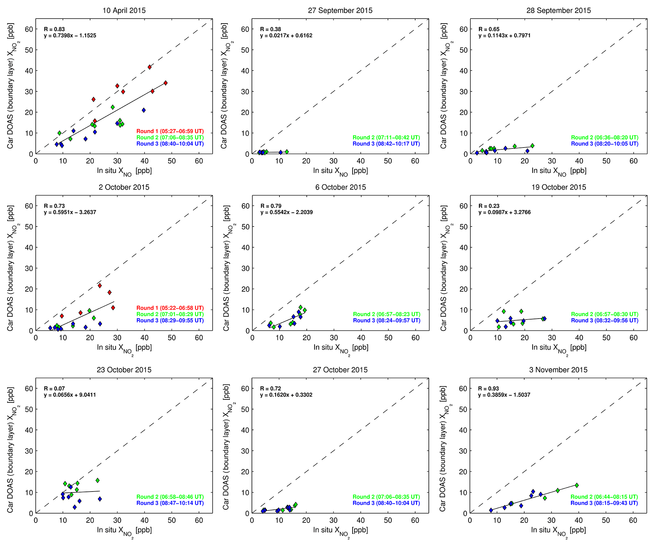
Figure 16Comparison of boundary layer NO2 mixing ratios estimated from car DOAS zenith-sky measurements with NO2 mixing ratios obtained from in situ measurements on the nine days when measurements were performed. The dotted line represents the 1:1 relationship.
Another explanation of the rather underestimated mixing ratio values obtained from car DOAS zenith-sky measurements observed on the other days is a possible overestimation of tropospheric AMFs, which are used for the conversion of NO2 DSCDs (see Eq. 1). Wang et al. (2012) have reported total uncertainties of tropospheric AMFs in the range of 20 %–30 % for SZAs < 40∘. With increasing SZA towards sunrise and sunset the uncertainties further increase. We note that most of our car DOAS zenith-sky measurements were performed for SZAs larger than 40∘.
Kramer et al. (2008) performed a comparison between data from a concurrent MAX-DOAS (CMAX-DOAS) instrument and in situ instruments in the city of Leicester, England. They highlighted the fact that the relative positions of the in situ instruments to the streets affect the comparison. In contrast to their study, car DOAS zenith-sky measurements were performed along motorways in our study. Therefore, this effect can be partly ruled out for the comparison presented in our study. Difficulties rather arise from losing some of the NO2 signal at the surface levels because of the zenith-sky geometry applied for our car DOAS measurements.
Nevertheless, large correlation coefficients (R = 0.72–0.93) are also observed on the other days with wind coming from the SE (6, 27 October and 3 November). In contrast, weak correlation between the two data sets is observed on days when wind was blowing from the NW (27 September, 19 and 23 October). The reason for the weak correlation on those days is not entirely clear. However, a closer look reveals that the variability of NO2 levels between the performed car journeys on a single day is only low on days with winds from the NW (see Table 3). This might be related to the high traffic volume but also most of the in situ monitoring stations used in this study are located rather in the SE of the city center than in the NW and thus the peak of rush-hour traffic does not show up in the measurements of most of the in situ monitoring stations on those days.
As values estimated via Eq. (3) represent averages within the PBL and thus values are rather underestimated when compared to the values obtained from air quality monitoring stations (see Table 3), a linear regression analysis is introduced (see Eq. 4). The motivation behind this approach is related to the findings of Dieudonné et al. (2013). The authors of that study highlighted the fact that the vertical distribution of NO2 within the PBL over an urban area is not homogenous. They also suggested considering the effect of wind speed on the vertical gradient. Therefore, we also include wind speed in the linear regression analysis.
The lap averages of car DOAS (surface) are given in Table 3. Overall, the values are in good agreement with the lap averages obtained from the air quality monitoring stations. For a better view, the modeled mixing ratios are plotted against mixing ratios obtained from in situ measurements in Fig. 17. The grey dotted lines represent the ±25 % level, meaning that all the values estimated via Eq. (4) are within ±25 %, with the exception of values lower than 10 ppb. The reason for these larger differences could be a reduced signal-to-noise ratio of the car DOAS zenith-sky measurements and consequently larger errors in the NO2 DSCDs. Nevertheless, the high correlation coefficient of the linear relationship (R = 0.94) is promising, in particular when thinking of applying this method to NO2 VCDtropo obtained from long-term MAX-DOAS measurements, which provide better statistics.
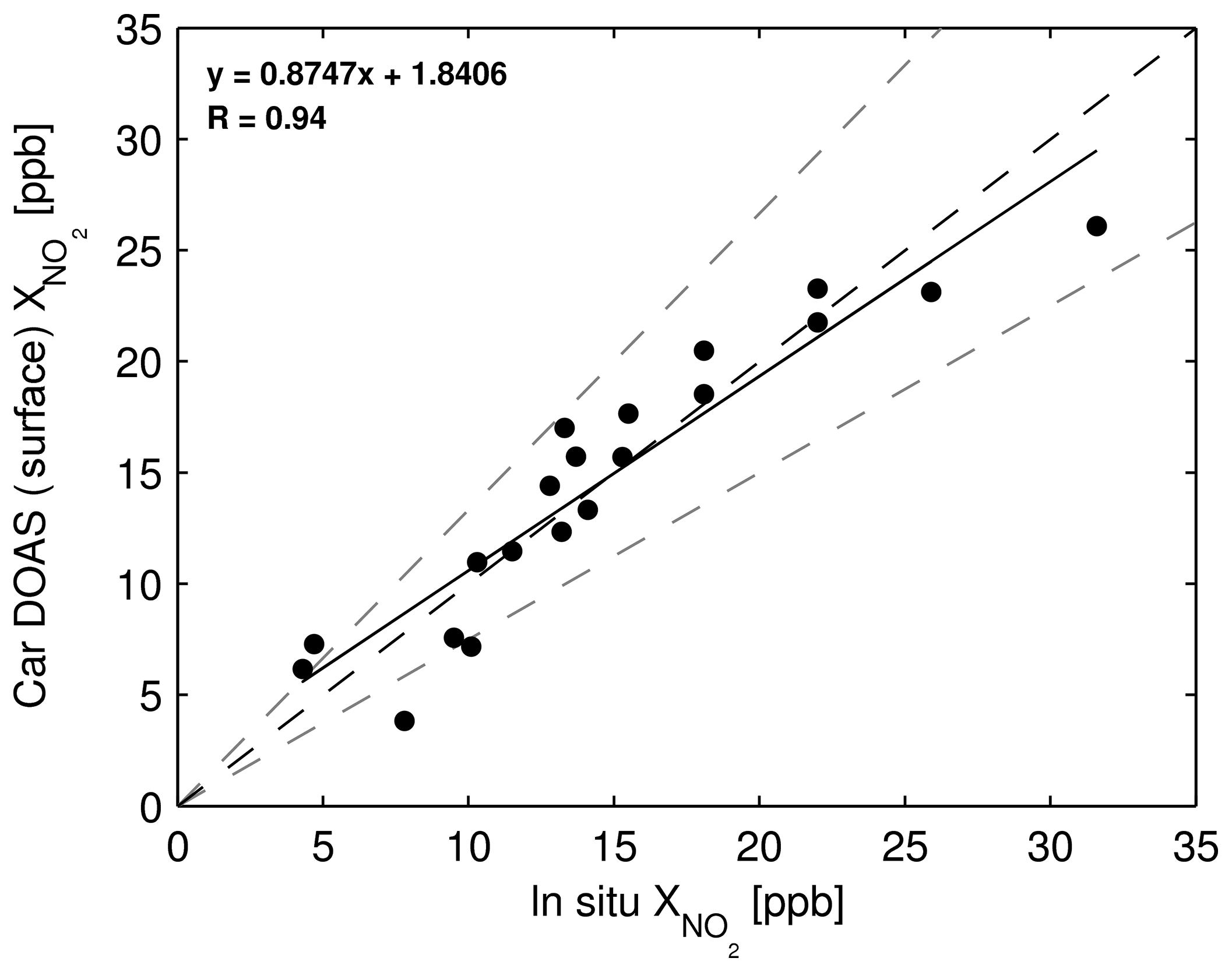
Figure 17Comparison of lap-averaged near-surface NO2 mixing ratios estimated from car DOAS zenith-sky measurements with NO2 mixing ratios obtained from in situ measurements. Lap averages of all 20 performed car rides are included in the calculation. The black and grey dotted lines represent the 1:1 relationship and ±25 %, respectively.
4.5 Path-averaged NO2 mixing ratios obtained from tower DOAS off-axis measurements
Although the NO2∕O4 ratio gives an overall impression of spatiotemporal changes of NO2 amounts over Vienna, an absolute quantification of NO2 amounts (e.g., the conversion into mixing ratios) is not possible with this approach. Therefore, another method is used for the estimation of path-averaged NO2 mixing ratios at 160 m altitude of the rotating tower platform (see Sect. 3.7.2).
Estimated horizontal optical path lengths as a function of the azimuthal viewing direction obtained from measurements taken on 29 April (blue) and 9 May (red) 2016 are shown in Fig. 18. Both curves represent the last round measurements recorded during those days, when the reference zenith-sky measurement was taken shortly afterwards. Overall, higher hOPLs are observed on 9 May, which was a day with wind speeds reaching up to 15 km h−1. The exceptionally low wind speeds observed on 29 April (< 5 km h−1) explain the lower values of hOPL on that day. Low values of hOPL are generally linked to low visibility, which is the result of an increased aerosol accumulation over emission hot spots on that otherwise cloudless day. As aerosols largely affect hOPL under such conditions (Sinreich et al., 2013), it is reasonable that the lowest values (5–6 km) are preferably found in off-axis directions between the eastern and southern directions, which include areas with high traffic roads and industry. In contrast, the highest hOPLs are observed in the north of the Vienna Danube Tower on both days (10–11 km). This is reasonable because those regions are known as rather rural areas without significant emission sources. The highest hOPLs estimated in our study are slightly lower than the mean value (12.9 km) reported in Seyler et al. (2017), but still within the standard deviation.

Figure 18Estimated horizontal optical path length (hOPL) obtained from tower DOAS off-axis measurements recorded during two tower platform rotations on 29 April and 9 May 2016.
Although our assumption made on the limitation of the horizontal light path length towards the hill might be critical, we argue that the distance of 6.95 km between the Vienna Danube Tower and the summit of that hill is still lower than 12.9±4.5 km and thus seems to be optimal for this normalization approach.
Estimated path-averaged NO2 mixing ratios are shown for 29 April (blue) and 9 May (red) 2016 in Fig. 19. Again, only the last rotations of those days are presented in the graph. As expected from the observed wind conditions and estimated hOPLs, path-averaged is higher on 29 April. Over rural areas, which are located in the north of the Vienna Danube Tower, values are lowest (2.5 to 4 ppb) on both days. In contrast, the highest values (up to 9 ppb) are again observed towards the SE. We note that path-averaged mixing ratios are only shown for two tower rotations, which took place shortly before noon – at a time when the peak in NO2 amounts over the city is past.
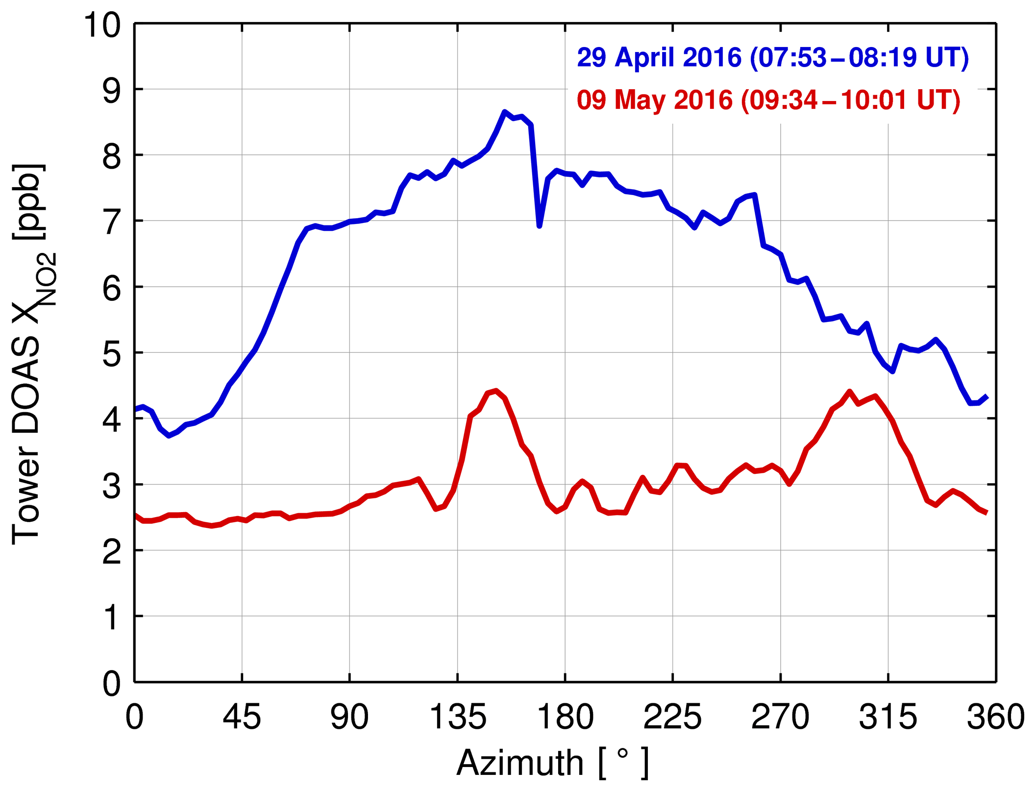
Figure 19Estimated path-averaged NO2 mixing ratios obtained from tower DOAS off-axis measurements recorded during two tower platform rotations on 29 April and 9 May 2016.
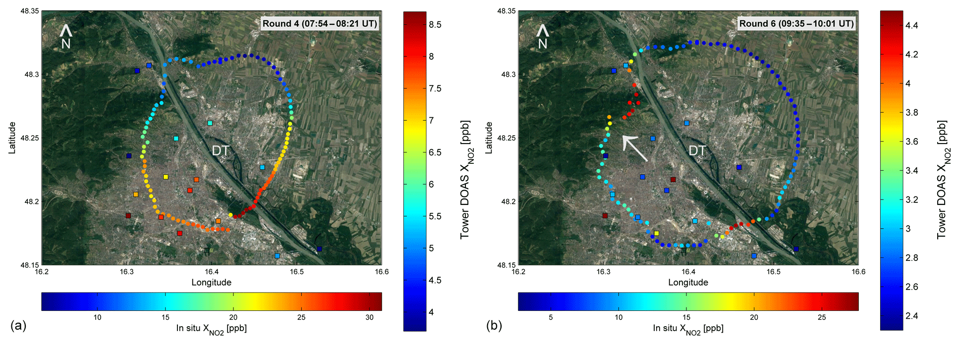
Figure 20Spatial variability of in Vienna based on tower DOAS off-axis (dots) and in situ surface measurements (squares) obtained on 29 April (a) and 9 May 2016 (b).
For a better illustration, as a function of hOPL obtained from the last rotation of tower DOAS off-axis measurements and values calculated from simultaneous in situ measurements are plotted on a geographical map in Fig. 20 for 29 April (a) and 9 May 2016 (b). We note that the NO2 mixing ratios estimated from tower DOAS off-axis measurements are averages over several kilometers at 160 m above ground, whereas NO2 mixing ratios from in situ stations rather represent point measurements at the surface level. The comparison therefore implies that the variability of NO2 as observed at 160 m above ground is much less pronounced than that between the individual ground stations. Moreover, horizontal gradients at 160 m above ground are small. As already outlined above, the highest NO2 amounts obtained from both measurements are generally found over the city center and over high-traffic roads in the southeast of the city center on 29 April, a day with very low wind speeds (< 5 km h−1). The picture looks different for 9 May, when wind was blowing from the southeast and wind speeds reached values of up to 15 km h−1. The highest NO2 amounts from tower DOAS off-axis observations are found in parallel to the wind direction in this case.

Figure 21Averaged from tower DOAS off-axis measurements as a function of averaged in situ surface on 29 April (blue) and 9 May (red) 2016. The mean and standard deviation of the former are calculated for round 4 (29 April) and round 6 (9 May), whereas mean and standard deviation of the latter are calculated from measurements of in situ stations falling within the circle determined by hOPL of the individual tower DOAS off-axis measurements (see Fig. 20).
For a better quantification, from tower DOAS off-axis measurements as well as from in situ observations are averaged and compared with each other (Fig. 21). While the mean and standard deviation are calculated by including all individual measurements of the last tower rotations in the former case, these parameters are computed by including measurements of from air quality monitoring stations that fall within the outer circle of tower DOAS off-axis measurements as determined by hOPL in the latter case. For both tower DOAS off-axis and in situ measurements, averaged values are larger by a factor of 2 on 29 April than on 9 May. On both days, averaged NO2 mixing ratios are about a factor of 6.5 larger at the surface level when compared with averaged path-averaged values at 160 m above the ground. This difference is much larger than the 25 % difference reported in Dieudonné et al. (2013), who compared surface concentrations with in situ concentrations at 300 m above ground in Paris. One reason for the larger factor found in our study might be an overestimation of mean at the surface level due to the relatively large number of air quality monitoring stations close to the city center, where higher pollution levels are expected. Conversely, low values of mean at 160 m above ground arise from the long light paths, which partly include areas with lower traffic density, especially in the north of the Danube River. Although a quantification and comparison is challenging for this case study with only a small number of data, interesting insights into NO2 distributions in the boundary layer above the urban area of Vienna can be gained.
In this case study, ground-based remote-sensing measurements have been coupled with surface in situ measurements to investigate the NO2 distributions in the planetary boundary layer in the Viennese metropolitan area.
A DOAS instrument was used for the determination of the spatial and temporal NO2 distributions in and around the urban area of Vienna. The instrument was applied in two different measurement setups: car DOAS zenith-sky and tower DOAS off-axis measurements. The former DOAS-type approach, which is already well-established and documented in the literature, was used for a total of 20 identical car journeys, which were carried out on nine days in April, September, October, and November 2015 during the morning hours. The latter configuration is innovative in the sense that horizontal measurements for more than 100 azimuthal angles are possible within a 360∘ rotation and within less than half an hour. The latter setup was used for collecting more than 30 rotations of spectral measurements on five days in April and May 2016.
A DOAS fitting procedure, based on recommendations made for the CINDI-2 campaign (http://www.tropomi.eu/, last access: 29 April 2019), is applied to the collected spectral measurements to retrieve NO2 DSCDs. Overall, good fit quality is found for both DOAS-type measurements, in particular when NO2 amounts were high.
As the car DOAS zenith-sky measurements include a contribution from both the background and stratospheric NO2, a correction scheme based on measurements and chemical transport model simulations is applied. The subsequent conversion of NO2 DSCDs into NO2 VCDtropo is performed by applying stratospheric and tropospheric AMFs as derived from radiative transfer calculations.
In order to correct light path lengths in the troposphere, NO2 DSCDs obtained from tower DOAS off-axis observations are normalized with O4 DSCDs in a first step. In a second step, the assumption that the Kahlenberg (484 m a.s.l.) limits the horizontal optical light path length at an azimuth angle of 305∘ is made. The distance between the Vienna Danube Tower and the summit of Kahlenberg (6.95 km) is then used for the normalization of O4 DSCDs to obtain horizontal optical path lengths (hOPLs).
By analyzing NO2 DSCDs at high temporal resolution along the individual car journeys, characteristic horizontal NO2 changes as a function of distance could be derived. While the absolute differences between the first and consecutive measurements increase sharply over the first two kilometers (by a factor of 1.5 to 4), the observed increase clearly weakens during the remaining kilometers. From this observation we conclude that 1–2 km is a characteristic scale of the NO2 fields observed in Vienna during the morning hours.
The analysis of NO2 VCDtropo from car DOAS zenith-sky measurements and DSCD NO2∕O4 from tower DOAS off-axis measurements opened up interesting insights into the spatial and temporal variations in NO2. The results imply that wind speed and wind direction impact strongly on the NO2 distributions in Vienna. By using data on wind speed and wind direction from several stations within the metropolitan area of Vienna, short-scale NO2 transport events could be identified.
The comparison of VCDtropo from car DOAS zenith-sky measurements with in situ NO2 concentrations, which is based on the conversion of both quantities into mixing ratios of NO2, revealed good linear correlation for days when the wind was blowing from the southeast (R = 0.73–0.93). In contrast, weak correlation was found for days when the wind was blowing from the northwest (R<0.38), which might be related to the overall cleaner air masses leading to lower sensitivity and larger uncertainties in the observations.
Depending on wind conditions, lap averages of near-surface NO2 mixing ratios () estimated from car DOAS zenith-sky measurements applying a linear regression analysis are in the range of 3.8 to 26.1 ppb and in good agreement with obtained from in situ measurements. The linear regression analysis, which is introduced for the first time and tested for the case-study-based data in this study, accounts for wind speed, in addition to mixing height (MH) and number density of air na.
Taking into account all the assumptions that have been made for the conversion of DSCDs into VCDtropo and also for the subsequent translation of VCDtropo into , the linear regression analysis to derive near-surface mixing ratios seems to work well and a correlation coefficient of R = 0.94 between modeled and measured in situ NO2 mixing ratios is achieved – at least for the lap averages considered in this study.
The estimation of hOPL and from the tower DOAS off-axis measurements revealed interesting insights into an upper layer of the PBL, although only a few measurements are presented due to the lack of sequential zenith-sky measurements that could be taken as reference. Overall, averaged NO2 mixing ratios are about a factor of 6.5 larger at the surface level when compared with mean path-averaged values at 160 m altitude.
Although the NO2 hourly European maximum dose rate was not exceeded when measurements were taken, NO2 amounts in the urban environment of Vienna are substantial, in particular during morning hours and when wind speeds are low.
We note that the idea of performing tower DOAS off-axis measurements was born when car DOAS zenith-sky measurements were already taken. Due to other priorities and limited help at the time when tower DOAS off-axis measurements were recorded, car DOAS zenith-sky measurements could not be carried out simultaneously. For future campaigns in Vienna, however, simultaneous measurements of the two DOAS configurations should be taken into consideration.
Future efforts will be made to test the linear regression analysis on measurements from three static MAX-DOAS instruments, which are located in Vienna as part of the VINDOBONA (VIenna horizontal aNd vertical Distribution OBservations Of Nitrogen dioxide and Aerosols) project (http://www.doas-vindobona.at, last access: 29 April 2019). Once the method is mature and optimized, it could also be applied to satellite measurements of VCDtropo. This would help to obtain near-surface mixing ratios of NO2 from the integrated column amounts on a global scale.
Additional car DOAS zenith-sky and tower DOAS off-axis measurements that complement the operational performance of the two MAX-DOAS instruments are also foreseen in the future. Taking these measurements and also data from the relatively large number of air quality monitoring stations into consideration, Vienna can be seen as an optimal urban location for future satellite validation campaigns.
Data can be requested from the corresponding author (stefan.schreier@boku.ac.at).
SFS, AR, and JPB formulated the overarching goals of this study. SFS and AR took the measurements. SFS and AR analyzed the data. SFS prepared the paper with contributions from AR and JPB.
The authors declare that they have no conflict of interest.
This study was funded by the University of Bremen and the Austrian Science Fund (FWF): I 2296-N29. We would like to thank “Amt der Niederösterreichischen Landesregierung” and “Amt der Wiener Landesregierung” for making the air quality data freely available. We wish to acknowledge the provision of meteorological data by the Austrian official weather service (ZAMG). Christoph Lotteraner and Martin Piringer (ZAMG) are acknowledged for calculating time series of mixing height at Vienna and Hohe Warte. We thank Andreas Hilboll (MARUM-Bremen) for the provision of simulated stratospheric NO2 amounts. Last but not least, we want to thank Mario Meyer and the staff from the Vienna Danube Tower for giving us the opportunity to perform experimental measurements from the rotating café and for providing technical assistance.
This paper was edited by Michael Pitts and reviewed by three anonymous referees.
Chipperfield, M. P.: Multiannual simulations with a three-dimensional chemical transport model, J. Geophys. Res., 104, 1781–1805, 1999.
Constantin, D. E., Merlaud, A., Van Roozendael, M., Voiculescu, M., Fayt, C., Hendrick, F., Pinardi, G., and Georgescu, L.: Measurements of tropospheric NO2 in Romania using a zenith–sky mobile DOAS system and comparisons with satellite observations, Sensors, 13, 3922–3940, 2013.
Danckaert, T., Fayt, C., van Roozendael, M., de Smedt, I., Letocart,V., Merlaud, A., and Pinardi, G.: QDOAS Software user manual, available at: http://uv-vis.aeronomie.be/software/QDOAS/QDOAS_manual.pdf (last access: 31 August 2016), 2015.
Dee, D. P., Uppala, S. M., Simmons, A. J., Berrisford, P., Poli, P., Kobayashi, S., Andrae, U., Balmaseda, M. A., Balsamo, G., Bauer, P., Bechtold, P., Beljaars, A. C. M., van de Berg, L., Bidlot, J., Bormann, N., Delsol, C., Dragani, R., Fuentes, M., Geer, A. J., Haimberger, L., Healy, S. B., Hersbach, H., Hólm, E. V., Isaksen, L., Kållberg, P., Köhler, M., Matricardi, M., McNally, A. P., Monge-Sanz, B. M., Morcrette, J.-J., Park, B.-K., Peubey, C., de Rosnay, P., Tavolato, C., Thépaut, J.-N., and Vitart, F.: The ERA-Interim reanalysis: configuration and performance of the data assimilation system, Q. J. Roy. Meteorol. Soc., 137, 553–597, https://doi.org/10.1002/qj.828, 2011.
Dieudonné, E., Ravetta, F., Pelon, J., Goutail, F., and Pommereau, J.-P.: Linking NO2 surface concentration and integrated content in the urban developed atmospheric boundary layer, Geophys. Res. Lett., 40, 1247–1251, https://doi.org/10.1002/grl.50242, 2013.
Dockery, D. W., Pope, A., Xu, X., Spengler, J. D., Ware, J. H., Fay, M., E., Ferris, B. J., and Speizer, F. E.: An association between air pollution and mortality in six US cities, New Eng. J. Med., 329, 1753–1759, 1993.
Dragomir, C. M., Constantin, D.-E., Voiculescu, M., Georgescu, L. P., Merlaud, A., and van Roozendael, M.: Modeling results of atmospheric dispersion of NO2 in an urban area using METI–LIS and comparison with coincident mobile DOAS measurements, Atmos. Pollut. Res., 6, 503–510, 2015.
Fontjin, A., Sabadell, A. J., and Ronco, R. J.: Homogeneous chemiluminescence measurement of nitric oxide with ozone, Anal. Chem., 42, 575–579, 1970.
Frins, E., Bobrowski, N., Osorio, M., Casaballe, N., Belsterli, G., Wagner, T., and Platt, U.: Scanning and mobile multi-axis DOAS measurements of SO2 and NO2 emissions from an electric power plant in Montevideo, Uruguay, Atmos. Environ., 98, 347–356, https://doi.org/10.1016/j.atmosenv.2014.03.069, 2014.
Gomez, L., Navarro-Comas, M., Puentedura, O., Gonzalez, Y., Cuevas, E., and Gil-Ojeda, M.: Long-path averaged mixing ratios of O3 and NO2 in the free troposphere from mountain MAX-DOAS, Atmos. Meas. Tech., 7, 3373–3386, https://doi.org/10.5194/amt-7-3373-2014, 2014.
Heue, K.-P., Richter, A., Bruns, M., Burrows, J. P., v. Friedeburg, C., Platt, U., Pundt, I.,Wang, P., and Wagner, T.: Validation of SCIAMACHY tropospheric NO2-columns with AMAXDOAS measurements, Atmos. Chem. Phys., 5, 1039–1051, https://doi.org/10.5194/acp-5-1039-2005, 2005.
Hilboll, A., Richter, A., and Burrows, J. P.: Long-term changes of tropospheric NO2 over megacities derived from multiple satellite instruments, Atmos. Chem. Phys., 13, 4145–4169, https://doi.org/10.5194/acp-13-4145-2013, 2013.
Hong, Q., Liu, C., Chan, K. L., Hu, Q., Xie, Z., Liu, H., Si, F., and Liu, J.: Ship-based MAX-DOAS measurements of tropospheric NO2, SO2, and HCHO distribution along the Yangtze River, Atmos. Chem. Phys., 18, 5931–5951, https://doi.org/10.5194/acp-18-5931-2018, 2018.
Hönninger, G., von Friedeburg, C., and Platt, U.: Multi axis differential optical absorption spectroscopy (MAX-DOAS), Atmos. Chem. Phys., 4, 231–254, https://doi.org/10.5194/acp-4-231-2004, 2004.
Ibrahim, O., Shaiganfar, R., Sinreich, R., Stein, T., Platt, U., and Wagner, T.: Car MAX-DOAS measurements around entire cities: quantification of NOx emissions from the cities of Mannheim and Ludwigshafen (Germany), Atmos. Meas. Tech., 3, 709–721, https://doi.org/10.5194/amt-3-709-2010, 2010.
Ionov, D. and Poberovskii, A.: Quantification of NOx emission from St Petersburg (Russia) using mobile DOAS measurements around the entire city, Int. J. Remote Sens., 36, 2486–2502, https://doi.org/10.1080/01431161.2015.1042123, 2015.
IPCC: Climate Change 2013: The Physical Science Basis, contribution of Working Group I to the Fifth Assessment Report of the Intergovernmental Panel on Climate Change, edited by: Stocker, T. F., Qin, D., Plattner, G.-K., Tignor, M., Allen, S. K., Boschung, J., Nauels, A., Xia, Y., Bex, V., and Midgley, P. M., Cambridge Univ. Press, Cambridge, UK and New York, NY, USA, 2013.
Johansson, M., Galle, B., Yu, T., Tang, L., Chen, D., Li, H., Li, J. X., and Zhang, Y.: Quantification 20 of total emission of air pollutants from Beijing using mobile mini-DOAS, Atmos. Environ. 42, 6926–6933, 2008.
Johansson, M., Rivera, C., de Foy, B., Lei, W., Song, J., Zhang, Y., Galle, B., and Molina, L.: Mobile mini-DOAS measurement of the outflow of NO2 and HCHO from Mexico City, Atmos. Chem. Phys., 9, 5647–5653, https://doi.org/10.5194/acp-9-5647-2009, 2009.
Knepp, T., Pippin, M., Crawford, J., Chen, G., Szykman, J., Long, R., Cowen, L., Cede, A., Abuhassan, N., Herman, J., Delgado, R., Compton, J., Berkoff, T., Fishman, J., Martins, D., Stauffer, R., Thompson, A. M., Weinheimer, A., Knapp, D., Montzka, D., Lenschow, D., and Neil, D.: Estimating surface NO2 and SO2 mixing ratios from fast-response total column observations and potential application to geostationary missions, J. Atmos. Chem., D15308, https://doi.org/10.1007/s10874-013-9257-6, 2013.
Kramer, L. J., Leigh, R. J., Remedios, J. J., and Monks, P. S.: Comparison of OMI and ground-based in situ and MAX-DOAS measurements of tropospheric nitrogen dioxide in an urban area, J. Geophys. Res., 113, D16S39, https://doi.org/10.1029/2007JD009168, 2008.
Künzli, N., Kaiser, R., Medina, S., Studnicka, M., Chanel, O., Filliger, P., Herry, M., Horak Jr, F., Puybonnieux-Texier, V., Quénel, P., Schneider, J., Seethaler, R., Vergnaud, J. C., and Sommer, H.: Public-health impact of outdoor and traffic-related air pollution: A European assessment, Lancet, 356, 795–801, 2000.
Kurucz, R. L., Furenhild, I., Brault, J., and Testermann, L.: Solar flux atlas from 296 to 1300 nm, National Solar Observatory Atlas No. 1, June 1984.
Lee, D. S., Köhler, I., Grobler, E., Rohrer, F., Sausen, R., Gallardo- Klenner, L., Olivier, J. G. J., Dentener, F. J., and Bouwman, A. F.: Estimations of global NO(x) emissions and their uncertainties, Atmos. Environ., 31, 1735–1749, 1997.
Lotteraner, C. and Piringer, M.: Mixing-Height Time Series from Operational Ceilometer Aerosol-Layer Heights, Bound.-Lay. Meteorol., 161, 265–287, https://doi.org/10.1007/s10546-016-0169-2, 2016.
Meier, A. C., Schönhardt, A., Bösch, T., Richter, A., Seyler, A., Ruhtz, T., Constantin, D.-E., Shaiganfar, R., Wagner, T., Merlaud, A., Van Roozendael, M., Belegante, L., Nicolae, D., Georgescu, L., and Burrows, J. P.: High-resolution airborne imaging DOAS measurements of NO2 above Bucharest during AROMAT, Atmos. Meas. Tech., 10, 1831–1857, https://doi.org/10.5194/amt-10-1831-2017, 2017.
Merlaud, A., Tack, F., Constantin, D., Georgescu, L., Maes, J., Fayt, C., Mingireanu, F., Schuettemeyer, D., Meier, A. C., Schönardt, A., Ruhtz, T., Bellegante, L., Nicolae, D., Den Hoed, M., Allaart, M., and Van Roozendael, M.: The Small Whiskbroom Imager for atmospheric compositioN monitorinG (SWING) and its operations from an unmanned aerial vehicle (UAV) during the AROMAT campaign, Atmos. Meas. Tech., 11, 551–567, https://doi.org/10.5194/amt-11-551-2018, 2018.
Nowlan, C. R., Liu, X., Janz, S. J., Kowalewski, M. G., Chance, K., Follette-Cook, M. B., Fried, A., González Abad, G., Herman, J. R., Judd, L. M., Kwon, H.-A., Loughner, C. P., Pickering, K. E., Richter, D., Spinei, E., Walega, J., Weibring, P., and Weinheimer, A. J.: Nitrogen dioxide and formaldehyde measurements from the GEOstationary Coastal and Air Pollution Events (GEO-CAPE) Airborne Simulator over Houston, Texas, Atmos. Meas. Tech., 11, 5941–5964, https://doi.org/10.5194/amt-11-5941-2018, 2018.
Ortega, I., Koenig, T., Sinreich, R., Thomson, D., and Volkamer, R.: The CU 2-D-MAX-DOAS instrument – Part 1: Retrieval of 3-D distributions of NO2 and azimuth-dependent OVOC ratios, Atmos. Meas. Tech., 8, 2371–2395, https://doi.org/10.5194/amt-8-2371-2015, 2015.
Perner, D. and Platt, U.: Detection of nitrous acid in the atmosphere by differential optical absorption, Geophys. Res. Lett., 6, 917–920, 1979.
Peters, E., Wittrock, F., Großmann, K., Frieß, U., Richter, A., and Burrows, J. P.: Formaldehyde and nitrogen dioxide over the remote western Pacific Ocean: SCIAMACHY and GOME-2 validation using ship-based MAX-DOAS observations, Atmos. Chem. Phys., 12, 11179–11197, https://doi.org/10.5194/acp-12-11179-2012, 2012.
Platt, U. and Stutz, J.: Differential Optical Absorption Spectroscopy. Physics of Earth and Space Environments, Springer, Berlin, 2008.
Richter, A., Burrows, J. P., Nüß, H., Granier, C., and Niemeier, U.: Increase in tropospheric nitrogen dioxide over China observed from space, Nature, 437, 129–132, https://doi.org/10.1038/nature04092, 2005.
Richter, A., Begoin, M., Hilboll, A., and Burrows, J. P.: An improved NO2 retrieval for the GOME-2 satellite instrument, Atmos. Meas. Tech., 4, 1147–1159, https://doi.org/10.5194/amt-4-1147-2011, 2011.
Rivera, C., Sosa, G., Whrnschimmel, H., de Foy, B., Johansson, M., and Galle, B.: Tula industrial complex (Mexico) emissions of SO2 and NO2 during the MCMA 2006 field campaign using a mobile mini-DOAS system, Atmos. Chem. Phys., 9, 6351–6361, https://doi.org/10.5194/acp-9-6351-2009, 2009.
Rivera, C., Barrera, H., Grutter, M., Zavala, M., Galle, B., Bei, N., Li, G., and Molina, L. T.: NO2 fluxes from Tijuana using a mobile mini-DOAS during Cal-Mex 2010, Atmos. Environ., 70, 532–539, 2013.
Roscoe, H. K., Van Roozendael, M., Fayt, C., du Piesanie, A., Abuhassan, N., Adams, C., Akrami, M., Cede, A., Chong, J., Clémer, K., Friess, U., Gil Ojeda, M., Goutail, F., Graves, R., Griesfeller, A., Grossmann, K., Hemerijckx, G., Hendrick, F., Herman, J., Hermans, C., Irie, H., Johnston, P. V., Kanaya, Y., Kreher, K., Leigh, R., Merlaud, A., Mount, G. H., Navarro, M., Oetjen, H., Pazmino, A., Perez-Camacho, M., Peters, E., Pinardi, G., Puentedura, O., Richter, A., Schönhardt, A., Shaiganfar, R., Spinei, E., Strong, K., Takashima, H., Vlemmix, T., Vrekoussis, M., Wagner, T., Wittrock, F., Yela, M., Yilmaz, S., Boersma, F., Hains, J., Kroon, M., Piters, A., and Kim, Y. J.: Intercomparison of slant column measurements of NO2 and O4 by MAX-DOAS and zenith-sky UV and visible spectrometers, Atmos. Meas. Tech., 3, 1629–1646, https://doi.org/10.5194/amt-3-1629-2010, 2010.
Rothman, L. S., Barbe, A., Benner, D. C., Brown, L. R., Camy-Peyret, C., Carleer, M. R., Chance, K., Clerbaux, C., Dana, V., Devi, V. M., Fayt, A., Flaud, J.-M., Gamache, R. R., Goldman, A., Jacquemart, D., Jucks, K. W., Lafferty, W. J., Mandin, J.-Y., Massie, S. T., Nemtchinov, V., Newnham, D. A., Perrin, A., Rinsland, C. P., Schroeder, J., Smith, K. M., Smith, M. A. H., Tang, K., Toth, R. A., Auwera, J. V., Varanasi, P., and Yoshino, K.: The HITRAN molecular spectroscopic database: edition of 2000 including updates through 2001, J. Quant. Spectr. Rad. Transf., 82, 5–44, 2003.
Rozanov, V., Rozanov, A., Kokhanovsky, A., and Burrows, J.: Radiative transfer through terrestrial atmosphere and ocean: Software package SCIATRAN, J. Quant. Spec. R. Trans., 133, 13–71, https://doi.org/10.1016/j.jqsrt.2013.07.004, 2014.
Schönhardt, A., Altube, P., Gerilowski, K., Krautwurst, S., Hartmann, J., Meier, A. C., Richter, A., and Burrows, J. P.: A wide field-of-view imaging DOAS instrument for two-dimensional trace gas mapping from aircraft, Atmos. Meas. Tech., 8, 5113–5131, https://doi.org/10.5194/amt-8-5113-2015, 2015.
Schreier, S. F., Peters, E., Richter, A., Lampel, J., Wittrock, F., and Burrows, J. P.: Ship-based MAX-DOAS measurements of tropospheric NO2 and SO2 in the South China and Sulu Sea, Atmos. Environ., 102, 331–343, https://doi.org/10.1016/j.atmosenv.2014.12.015, 2015.
Schreier, S. F., Richter, A., Wittrock, F., and Burrows, J. P.: Estimates of free-tropospheric NO2 and HCHO mixing ratios derived from high-altitude mountain MAX-DOAS observations at midlatitudes and in the tropics, Atmos. Chem. Phys., 16, 2803–2817, https://doi.org/10.5194/acp-16-2803-2016, 2016.
Serdyuchenko, A., Gorshelev, V., Weber, M., Chehade, W., and Burrows, J. P.: High spectral resolution ozone absorption cross-sections – Part 2: Temperature dependence, Atmos. Meas. Tech., 7, 625–636, https://doi.org/10.5194/amt-7-625-2014, 2014.
Seyler, A., Wittrock, F., Kattner, L., Mathieu-Üffing, B., Peters, E., Richter, A., Schmolke, S., and Burrows, J. P.: Monitoring shipping emissions in the German Bight using MAX-DOAS measurements, Atmos. Chem. Phys., 17, 10997–11023, https://doi.org/10.5194/acp-17-10997-2017, 2017.
Shaiganfar, R., Beirle, S., Sharma, M., Chauhan, A., Singh, R. P., and Wagner, T.: Estimation of NOx emissions from Delhi using Car MAX-DOAS observations and comparison with OMI satellite data, Atmos. Chem. Phys., 11, 10871–10887, https://doi.org/10.5194/acp-11-10871-2011, 2011.
Sinnhuber, B.-M., Weber, M., Amankwah, A., and Burrows, J. P.: Total ozone during the unusual Antarctic winter of 2002, Geophys. Res. Lett., 30, 1580–1584, https://doi.org/10.1029/2002GL016798, 2003a.
Sinnhuber, M., Burrows, J. P., Chipperfield, M. P., Jackman, C. H., Kallenrode, M.-B., Künzi, K. F., and Quack, M.: A model study of the impact of magnetic field structure on atmospheric composition during solar proton events, Geophys. Res. Lett., 30, 1818–1821, https://doi.org/10.1029/2003GL017265, 2003b.
Sinreich, R., Merten, A., Molina, L., and Volkamer, R.: Parameterizing radiative transfer to convert MAX-DOAS dSCDs into near-surface box-averaged mixing ratios, Atmos. Meas. Tech., 6, 1521–1532, https://doi.org/10.5194/amt-6-1521-2013, 2013.
Spangl, W.: Luftgütemessstellen in Österreich, REPORT REP 0607, Umweltbundesamt GmbH, Wien, 2017.
Spangl, W. and Nagl, C.: Jahresbericht der Luftgütemessungen in Österreich 2015, REPORT REP-0562, Umweltbundesamt GmbH, Wien, 2016.
Tack, F., Hendrick, F., Goutail, F., Fayt, C., Merlaud, A., Pinardi, G., Hermans, C., Pommereau, J.-P., and Van Roozendael, M.: Tropospheric nitrogen dioxide column retrieval from ground-based zenith–sky DOAS observations, Atmos. Meas. Tech., 8, 2417–2435, https://doi.org/10.5194/amt-8-2417-2015, 2015.
Tack, F., Merlaud, A., Iordache, M.-D., Danckaert, T., Yu, H., Fayt, C., Meuleman, K., Deutsch, F., Fierens, F., and Van Roozendael, M.: High-resolution mapping of the NO2 spatial distribution over Belgian urban areas based on airborne APEX remote sensing, Atmos. Meas. Tech., 10, 1665–1688, https://doi.org/10.5194/amt-10-1665-2017, 2017.
Takashima, H., Irie, H., Kanaya, Y., and Syamsudin, F.: NO2 observations over the western Pacific and Indian Ocean by MAX-DOAS on Kaiyo, a Japanese research vessel, Atmos. Meas. Tech., 5, 2351–2360, https://doi.org/10.5194/amt-5-2351-2012, 2012.
Thalman, R. and Volkamer, R.: Temperature dependent absorption cross-sections of O2-O2 collision pairs between 340 and 630 nm and at atmospherically relevant pressure, Phys. Chem. Chem. Phys., 15, 15371–15381, https://doi.org/10.1039/c3cp50968k, 2013.
Vandaele, A. C., Hermans, C., Simon, P. C., Roozendael, M. V., Guilmot, J. M., Carleer, M., and Colin, R.: Fourier transform measurement of NO2 absorption cross-section in the visible range at room temperature, J. Atmos. Chem., 25, 289–305, 1996.
Wagner, T., Ibrahim, O., Shaiganfar, R., and Platt, U.: Mobile MAX-DOAS observations of tropospheric trace gases, Atmos. Meas. Tech., 3, 129–140, https://doi.org/10.5194/amt-3-129-2010, 2010.
Wang, P., Richter, A., Bruns, M., Rozanov, V. V., Burrows, J. P., Heue, K.-P.,Wagner, T., Pundt, I., and Platt, U.: Measurements of tropospheric NO2 with an airborne multi-axis DOAS instrument, Atmos. Chem. Phys., 5, 337–343, https://doi.org/10.5194/acp-5-337-2005, 2005.
Wang, S., Zhou, B., Wang, Z., Yang, S., Hao, N., Valks, P., Trautmann, T., and Chen, L.: Remote Sensing of NO2 Emission from the Central Urban Area of Shanghai (China) Using the Mobile DOAS Technique, J. Geophys. Res., 117, D13305, https://doi.org/10.1029/2011JD016983, 2012.
WHO: Health Aspects of Air Pollution with Particulate Matter, Ozone and Nitrogen Dioxide, World Health Organization, Bonn, 2003.
Winkler, H., Sinnhuber, M., Notholt, J., Kallenrode, M.-B., Steinhilber, F., Vogt, J., Zieger, B., Glassmeier, K.-H., and Stadelmann, A.: Modeling impacts of geomagnetic field variations on middle atmospheric ozone responses to solar proton events on long timescales, J. Geophys. Res., 113, D02302, https://doi.org/10.1029/2007JD008574, 2008.
Wittrock, F., Oetjen, H., Richter, A., Fietkau, S., Medeke, T., Rozanov, A., and Burrows, J. P.: MAX-DOAS measurements of atmospheric trace gases in Ny-Ålesund – Radiative transfer studies and their application, Atmos. Chem. Phys., 4, 955–966, https://doi.org/10.5194/acp-4-955-2004, 2004.
Wu, F. C., Xie, P. H., Li, A., Chan, K. L., Hartl, A., Wang, Y., Si, F. Q., Zeng, Y., Qin, M., Xu, J., Liu, J. G., Liu, W. Q., and Wenig, M.: Observations of SO2 and NO2 by mobile DOAS in the Guangzhou eastern area during the Asian Games 2010, Atmos. Meas. Tech., 6, 2277–2292, https://doi.org/10.5194/amt-6-2277-2013, 2013.