the Creative Commons Attribution 4.0 License.
the Creative Commons Attribution 4.0 License.
 | 12 Apr 2019
Identification of soil-cooling rains in southern France from soil temperature and soil moisture observations
Sibo Zhang
Catherine Meurey
Jean-Christophe Calvet
In this study, the frequency and intensity of soil-cooling rains is assessed using in situ observations of atmospheric and soil profile variables in southern France. Rainfall, soil temperature, and topsoil volumetric soil moisture (VSM) observations, measured every 12 min at 21 stations of the SMOSMANIA (Soil Moisture Observing System – Meteorological Automatic Network Integrated Application) network, are analyzed over a time period of 9 years, from 2008 to 2016. The spatial and temporal statistical distribution of the observed rainfall events presenting a marked soil-cooling effect is investigated. It is observed that the soil temperature at a depth of 5 cm can decrease by as much as 6.5 ∘C in only 12 min during a soil-cooling rain. We define marked soil-cooling rains as rainfall events triggering a drop in soil temperature at a depth of 5 cm larger than 1.5 ∘C in 12 min. Under Mediterranean and Mediterranean–mountain climates, it is shown that such events occur up to nearly 3 times a year, and about once a year on average. This frequency decreases to about once every 3.5 years under semi-oceanic climate. Under oceanic climate, such pronounced soil-cooling rains are not observed over the considered period of time. Rainwater temperature is estimated for 13 cases of marked soil-cooling rains using observed changes within 12 min in soil temperature at a depth of 5 cm, together with soil thermal properties and changes in VSM. On average, the estimated rainwater temperature is generally lower than the observed ambient air temperature, wet-bulb temperature, and topsoil temperature at a depth of 5 cm, with mean differences of −5.1, −3.8, and −11.1 ∘C, respectively. The most pronounced differences are attributed to hailstorms or to hailstones melting before getting to the soil surface. Ignoring this cooling effect can introduce biases in land surface energy budget simulations.
- Article
(2126 KB) -
Supplement
(1817 KB) - BibTeX
- EndNote


Over natural and agricultural land surfaces, the frequency and intensity of rainfalls govern soil moisture dynamics from topsoil layers to the root zone. While these processes are represented in land surface models (LSMs) (e.g., Decharme et al., 2013), sensible heat input from liquid water into the soil and its impact on the soil temperature profile are often overlooked (Wang et al., 2016). For example, current versions of the ISBA (Interactions between Soil, Biosphere, and Atmosphere) LSM developed by Centre National de Recherches Météorologiques (CNRM) neglect the precipitation-induced sensible heat flux (PH). Rainwater temperature is rarely measured, and raindrop temperature is not explicitly simulated in atmospheric models (Wei et al., 2014).
The impact of neglecting this process was investigated in recent studies, in the context of global atmospheric simulations. Wang et al. (2016) showed that the impact on land surface temperature was relatively small in LMDZ simulations (less than 0.3 ∘C), but they considered mean annual air temperature differences only. Wei et al. (2014) showed that accounting for precipitation-induced sensible heat helps in reducing biases in land surface air temperature simulated by the Community Earth System Model 1 (CESM1). Focusing on the winter season in the Northern Hemisphere, they found a pronounced effect (up to 1 ∘C) on land surface air temperature in their simulations. In both studies, it was assumed that rainwater temperature was equal to the air wet-bulb temperature. This assumption is valid for raindrops in thermal equilibrium with the ambient air (Kinzer and Gunn, 1951). Both studies tended to show a soil-cooling effect over France, but for some regions at higher latitudes a soil-warming effect was simulated.
At the field scale, Kollet et al. (2009) simulated the impact of a rainfall event on soil temperature at a depth of 5 cm (T5 cm) over a grassland site in the Netherlands. They showed that accounting for precipitation-induced sensible heat in their simulations triggered a drop in T5 cm of more than 1 ∘C on a single rainfall event. The simulated surface energy fluxes were markedly influenced by this soil-cooling event during several days. In particular, the ground heat flux was affected during nearly 1 month. They suggested that this effect could be more pronounced in regions affected by strong convective rainfall events. They did not measure rainwater temperature, and they assumed that it was equal to the air wet-bulb temperature.
Rainwater temperature was measured in 1947 by Byers et al. (1949) at Wilmington, Ohio, USA. They analyzed the data from seven storms and concluded that three types of events could be distinguished according to rainwater temperature values within minutes after the rain onset: close to air temperature, close to wet-bulb temperature, and lower than air temperature by as much as 10 ∘C. They attributed the latter kind of event to hail melting before reaching the surface.
More than 70 years after Byers et al. (1949) performed their experiment, we were not able to find other examples in the open literature of the analysis of ground rainwater temperature observations. Such measurements are usually not performed in networks of ground meteorological stations.
The objectives of this study are to assess (1) the frequency of soil-cooling rains across contrasting climatic areas in southern France using in situ observations of atmospheric and soil profile variables, (2) the feasibility of estimating rainwater temperature using soil temperature profile measurements, and (3) the difference between rainwater temperature and the ambient air temperature or wet-bulb temperature and the topsoil temperature.
We use the in situ soil temperature and volumetric soil moisture (VSM) measurements collected by the SMOSMANIA (Soil Moisture Observing System – Meteorological Automatic Network Integrated Application) network in southern France (Calvet et al., 2007, 2016), over a 9-year time period from 2008 to 2016. The soil profile measurements are made at a high sampling frequency of one observation every 12 min, and the accumulated precipitation is available at the same frequency. This permits investigating intense precipitation events and their impact on topsoil variables, together with the retrieval of rainwater temperature in certain conditions.
The observations and the model simulations are presented in Sect. 2. Methods for selecting marked soil-cooling rains and for estimating rainwater temperature are described in Sect. 3. The statistical distribution of soil-cooling rains and estimates of rainwater temperature are presented in Sect. 4. The results are discussed in Sect. 5. The main conclusions are summarized together with prospects for further research in Sect. 6.
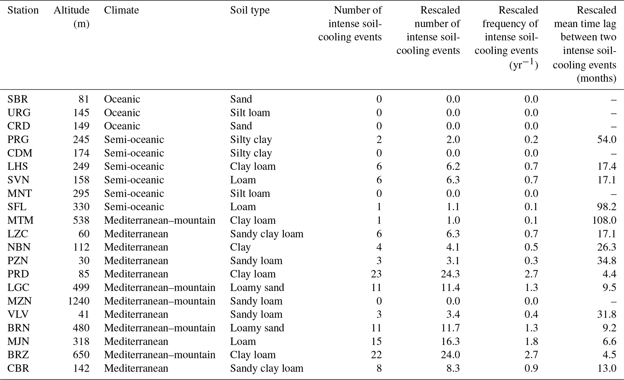
The SMOSMANIA network was implemented in southern France by Météo-France, the French national meteorological service, in order to monitor in situ soil moisture and soil temperature in contrasting soil and climatic conditions at operational automatic weather stations (Calvet et al., 2007). The SMOSMANIA network is composed of 21 stations forming an Atlantic–Mediterranean transect shown in Fig. 1. Soil and climate types for the 21 stations of the SMOSMANIA network are presented in Table 1. Station full names are given in Table S1 (see Supplement). The three westernmost stations are close to the Atlantic Ocean and present an oceanic climate. Further east, six stations present a semi-oceanic climate. The 12 easternmost stations are close to the Mediterranean Sea and present a Mediterranean climate. Among them, five are located at altitudes above sea level (a.s.l.) higher than 400 m a.s.l. over complex, mountainous terrain in the Corbières (MTM) and Cévennes (LGC, MZN, BRN, BRZ) mountainous areas. Two stations (MZN and BRZ) of the Cévennes area are located higher than 600 m a.s.l. and present lower mean monthly minimum and maximum temperatures (Tmin and Tmax, respectively) than the other stations. While Tmin can be 2 to 3 ∘C below freezing level at wintertime at MZN and BRZ, Tmin is always higher than 1 to 5 ∘C above freezing level at the other stations. The Tmax values do not exceed 21 and 24 ∘C at MZN and BRZ, respectively, while Tmax at the other stations can reach 26 to 30 ∘C. Oceanic, semi-oceanic, and Mediterranean climates are characterized by contrasting precipitation regimes, with maximum monthly precipitation occurring at wintertime, in spring, and in the autumn, respectively (see Sect. 4.1). It must be noted that Mediterranean stations are often affected by severe convective precipitation events such as thunderstorms and hailstorms, especially in the autumn (Ruti et al., 2016). This is true for stations located in mountainous areas, but also for those located in the foothills of Corbières (NBN), Cévennes (PZN, PRD, VLV, MJN), and Monts de Vaucluse (Vaucluse Mountains, CBR). Table 1 also presents the frequency of intense soil-cooling events (see Sects. 3 and 4). Since a noticeable fraction of observed T5 cm or VSM5 cm data is missing, the number of marked soil-cooling rainfall events could be underestimated. The missing data fraction across seasons (Table S1) is used to correct the estimation of the possible number of intense soil-cooling rainfall events, their frequency, and the mean time lag between two events in Table 1.
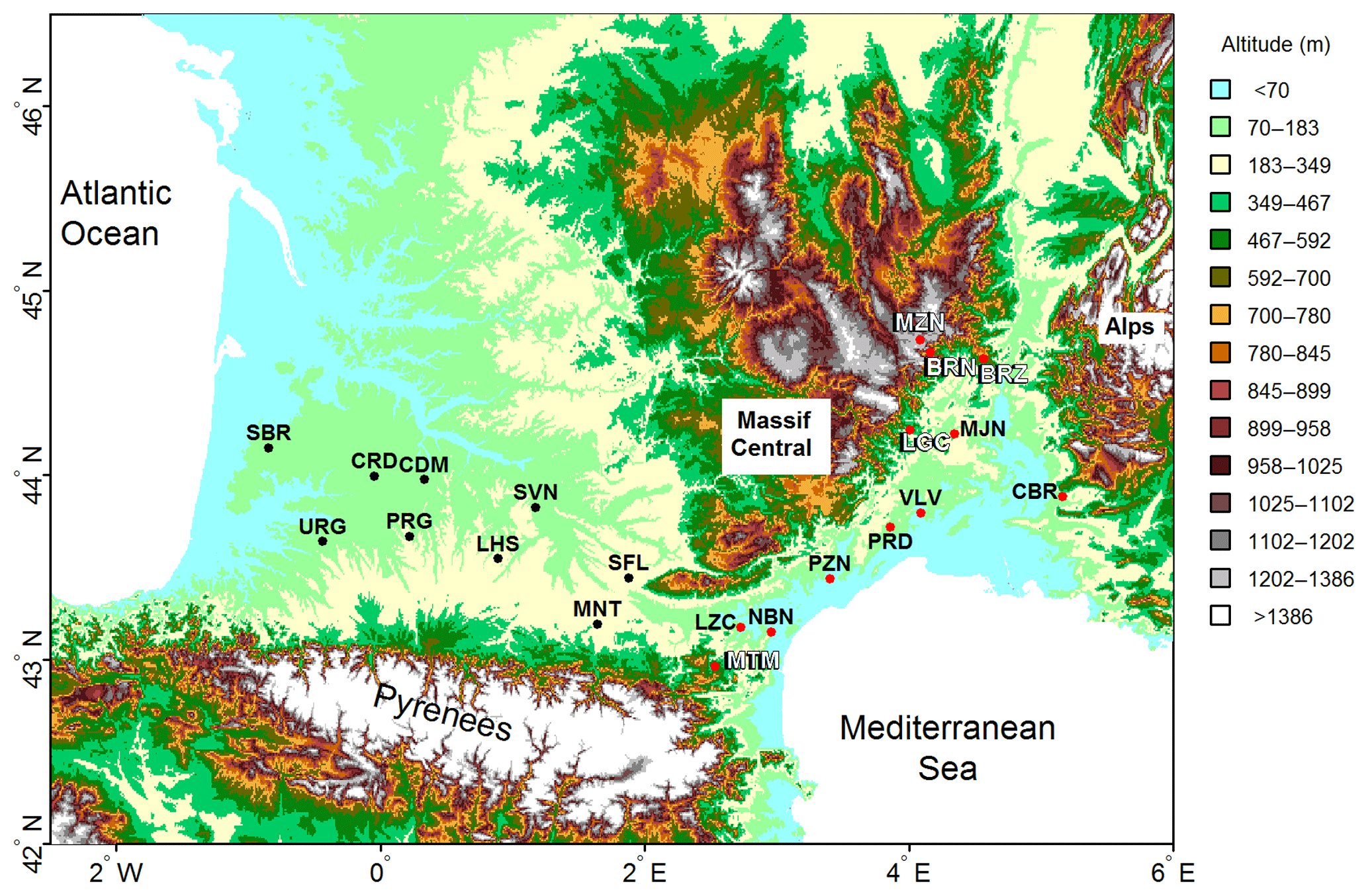
Figure 1Locations of the 21 SMOSMANIA stations in southern France. Black dots indicate stations under oceanic and semi-oceanic climates. Red dots indicate stations under Mediterranean and Mediterranean–mountain climates. White letters are for names of the five stations under Mediterranean–mountain climates. Background geographic altitudes are from SRTM 90 m digital elevation data (http://srtm.csi.cgiar.org/, last access: April 2019).
Table 1The environment characteristics for the 21 stations of the SMOSMANIA network and the frequency of intense soil cooling during marked rainfall events from 2008 to 2016. The number of intense soil-cooling rains, the frequency, and the mean time lag between two intense soil-cooling rains are rescaled according to the fraction of missing data across seasons (see Table S1). Stations are listed from (top) west to (bottom) east.
In general, the soil around the stations is covered by grass. The soil properties were measured for each station as described in Calvet et al. (2016). In the SMOSMANIA network, VSM and soil temperature are measured every 12 min at four depths (5, 10, 20, and 30 cm) using ThetaProbe and PT100 sensors, respectively. The soil moisture (temperature) observations are recorded with a resolution of 0.001 m3 m−3 (0.1 ∘C). The data are available to the research community through the International Soil Moisture Network website (ISMN, 2018). In this study, the sub-hourly observations of VSM and soil temperature were used over 9 years from 2008 to 2016.
Additionally, the SMOSMANIA network consists of preexisting automatic weather stations operated by Météo-France, measuring atmospheric variables. We used a number of meteorological observations such as the maximum and minimum air temperatures in an hour at 2 m, the hourly mean relative humidity (RH) of the air, and the accumulated rainfall every 12 min. A small fraction (less than 4 %) of the rainfall data is missing at each station. For most of the stations, a larger fraction of the VSM and soil temperature observations is missing. The mean fractions of missing data for all stations are 0.11 and 0.15 for VSM and T5 cm, respectively. The mean fraction of missing data for either VSM or T5 cm is 0.17. More details on missing data for each station, including the seasonal distribution of missing data, are given in Figs. S1, S2, and in Table S1 (see the Supplement). For stations presenting a fraction of missing data larger than 0.1, the fraction of missing data is relatively evenly distributed across seasons. Missing data are slightly more frequent at wintertime and in spring. The maximum fraction of missing VSM at 5 cm is 0.23 at the SBR station, and the maximum fraction of missing T5 cm is 0.47 at the VLV station (Fig. S1). The scaled missing data fraction of either VSM or T5 cm is shown in Fig. S2 and Table S1 for each season.
3.1 Identification of intense soil cooling
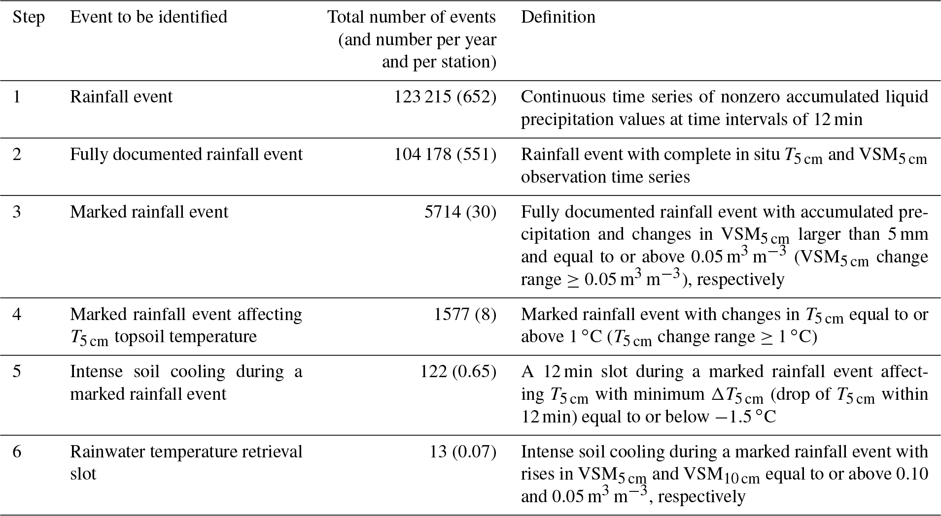
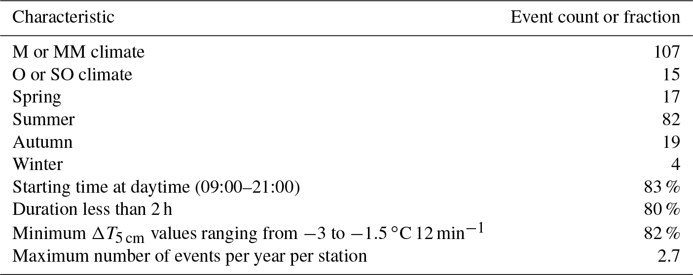
In situ rainfall observations are used to identify various types of rainfall events in six steps summarized in Table 2. In a first stage, a rainfall event is defined as a continuous time series of nonzero accumulated liquid precipitation values at time intervals of 12 min. Then we only keep the fully documented rainfall events with available soil temperature and VSM observations at a depth of 5 cm. Another stage of data sorting (step 3 in Table 2) is needed to ensure that rainwater is not completely intercepted by vegetation and is able to actually reach the soil. Because of the method used to count rainfall events, only about 5 % of the rainfall events exceed 5 mm and have a significant impact on the topsoil VSM. Among these marked rainfall events, we sort out (step 4) those affecting T5 cm by more than 1 ∘C. In order to assess the precipitation-induced sensible heat flux (PH) on the topsoil temperature, we then select marked soil-cooling rainfall events (step 5) presenting at least one marked drop of T5 cm of at least −1.5 ∘C in 12 min. No other meteorological factor can trigger such rapid changes in topsoil temperature.
Table 2Steps for identifying marked soil-cooling rains, together with the number of events for all the SMOSMANIA stations from 2008 to 2016.
Finally, a few cases are selected (step 6) for the assessment of the rainwater temperature retrieval (Sect. 3.2), in conditions where the topsoil VSM profile is sufficiently affected by the rainwater.
3.2 Estimation of rainwater temperature
In the SMOSMANIA network, rainwater temperature is not measured. We investigate whether it is realistic to postulate that the rainwater temperature can be estimated using in situ topsoil VSM5 cm and T5 cm observations within a topsoil layer of depth Δz=0.1 m. We focus on marked soil-cooling rainfall events corresponding to a drop in topsoil temperature associated with a rise in VSM values. This condition is not always satisfied in practice because the soil temperature probes and the soil moisture probes at a given soil depth are not located at exactly the same place. In order to limit the impact of spatial heterogeneities in the infiltration of rainwater into the soil, we consider intense precipitation events able to markedly wet the topsoil soil moisture (VSM5 cm) together with the deeper soil layer (VSM10 cm) during the drop in T5 cm. The in situ VSM observations at a depth of 10 cm (VSM10 cm) are used to ensure that the rainwater really penetrates into the soil and affects the topsoil layer as a whole. Among 122 rainfall events presenting intense soil cooling, 101 events have available VSM10 cm observations, and only 50 events present an increase in VSM10 cm larger than 0.05 m3 m−3. Within these 50 rainfall events, we only select 13 events for which the rise in VSM5 cm corresponds to the rise in VSM10 cm and to the drop in T5 cm within the same 12 min slot (step 6 in Table 2). Firstly, the soil heat capacity at a depth of 5 cm at time t (, in units of J m−3 K−1) is estimated using the volumetric soil moisture at a depth of 5 cm at time t, (in units of m3 m−3):
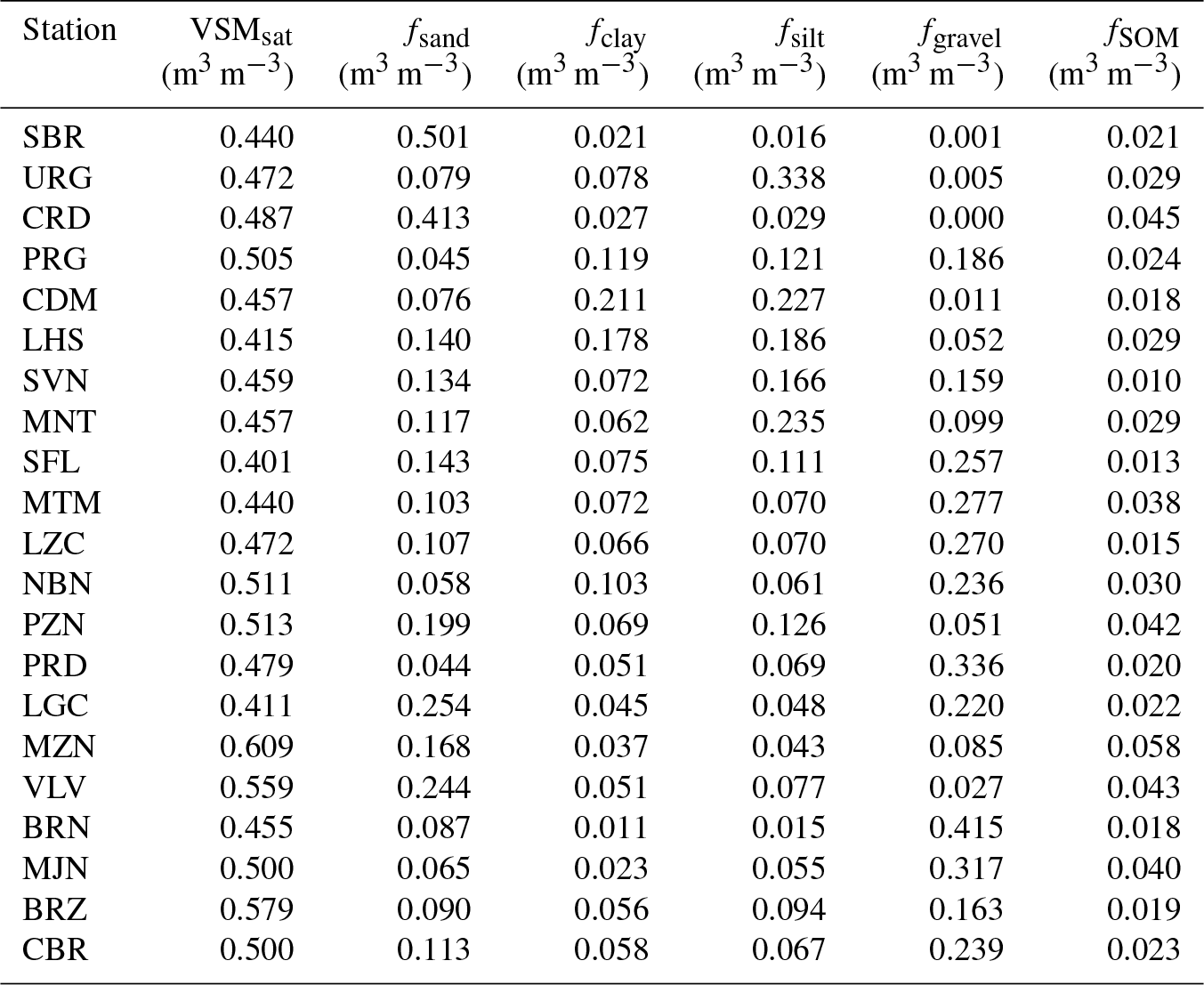
where Cwater, Cmin, and CSOM are heat capacity values of water, soil minerals, and soil organic matter (SOM) (4.2×10⁶, 2.0×10⁶, and 2.5×10⁶ J m−3 K−1, respectively). Their corresponding volumetric fractions at a depth of 5 cm (Table 3) are VSM, fmin, and fSOM. Soil minerals consist of sand, clay, silt, and gravels. Values of the VSM at saturation at a depth of 5 cm VSMsat (the porosity) are also listed in Table 3 for all stations. While the volumetric fractions of sand (fsand), clay (fclay), and silt (fsilt) were directly measured at a depth of 5 cm, the volumetric fraction of gravels (fgravel) was derived from measurements made at a depth of 10 cm (Sect. 5.1).
Table 3Soil characteristics at a depth of 5 cm for the 21 stations of the SMOSMANIA network. The volumetric fractions of sand, clay, and silt at 5 cm (fsand, fclay, and fsilt) are measured, and the volumetric fractions of gravel and soil organic matter (SOM) (fgravel and fSOM) at 5 cm are derived from measurements at 10 cm. VSMsat is the porosity representing VSM at saturation (VSM). Stations are listed from (top) west to (bottom) east.
During a short time period from time t1 to t2 (12 min in this study) of intense precipitation for which PH dominates heat exchanges in the topsoil layer, we can assume that the heat storage change in the topsoil layer, in units of J m−2, corresponds to the change in temperature of the infiltrated rainwater as
One may assume that soil and incoming rainwater have reached thermal equilibrium at time t2. Houpeurt et al. (1965) showed that thermal equilibrium is nearly instantaneous for small soil mineral particles (e.g., about 10 s or less for particle size of less than 5 mm). With this assumption, the rainwater temperature at time t2 () is equal to the measured soil temperature at time t2 (), and the rainwater temperature just before reaching the soil at time t1 () can be estimated as
It must be noted that Eqs. (2) and (3) are valid for liquid rainwater only. During hailstorms, hailstones can melt at the soil surface, and part of the heat extracted from the topsoil layer (left term in Eq. 2) is used for ice melting. Hailstones may melt after getting to the soil surface or just before. It can be assumed that both liquid water resulting from hailstones melting at the surface and liquid rainwater getting to the soil together with hailstones are very close to freezing level (Tf=0 ∘C) before infiltrating the topsoil layer. In this case, the quantity of hailstones (in kg m−2) melting after getting to the soil surface, I, can be estimated as
where J kg−1 is the latent heat of fusion. Since a fraction of the raindrops may exceed freezing temperature, I as calculated from Eq. (4) is a low estimate.
4.1 Identification of soil-cooling rains
The various types of rainfall events considered in this study are listed in Table 2. Their frequency is indicated. After data sorting (step 3 in Table 2), only 5.5 % of the fully documented rainfall events can be considered as marked rainfall events, with accumulated precipitation and changes in VSM5 cm larger than 5 mm and 0.05 m3 m−3, respectively. At the same time, this small fraction of rainfall events contributes as much as 57 % of the accumulated rainfall of all rainfall events. On average, 30 marked rainfall events are observed each year at each station.
Among these marked rainfall events, some have a notable impact on the soil temperature and soil moisture profiles. This is illustrated by Fig. 2, showing soil temperature and soil moisture measured at the PRD station from 21 to 25 August 2015 at depths of 5, 10, 20, and 30 cm. A sharp decrease in soil temperature associated with an increase in soil moisture can be observed around noon of 23 August 2015, along with a rainfall event. The most pronounced impacts of the rain are on the topsoil variables at a depth of 5 cm, but the whole soil profile is affected by the rain, down to a depth of 30 cm. This clearly shows the effects on soil temperature of a soil-cooling rain.
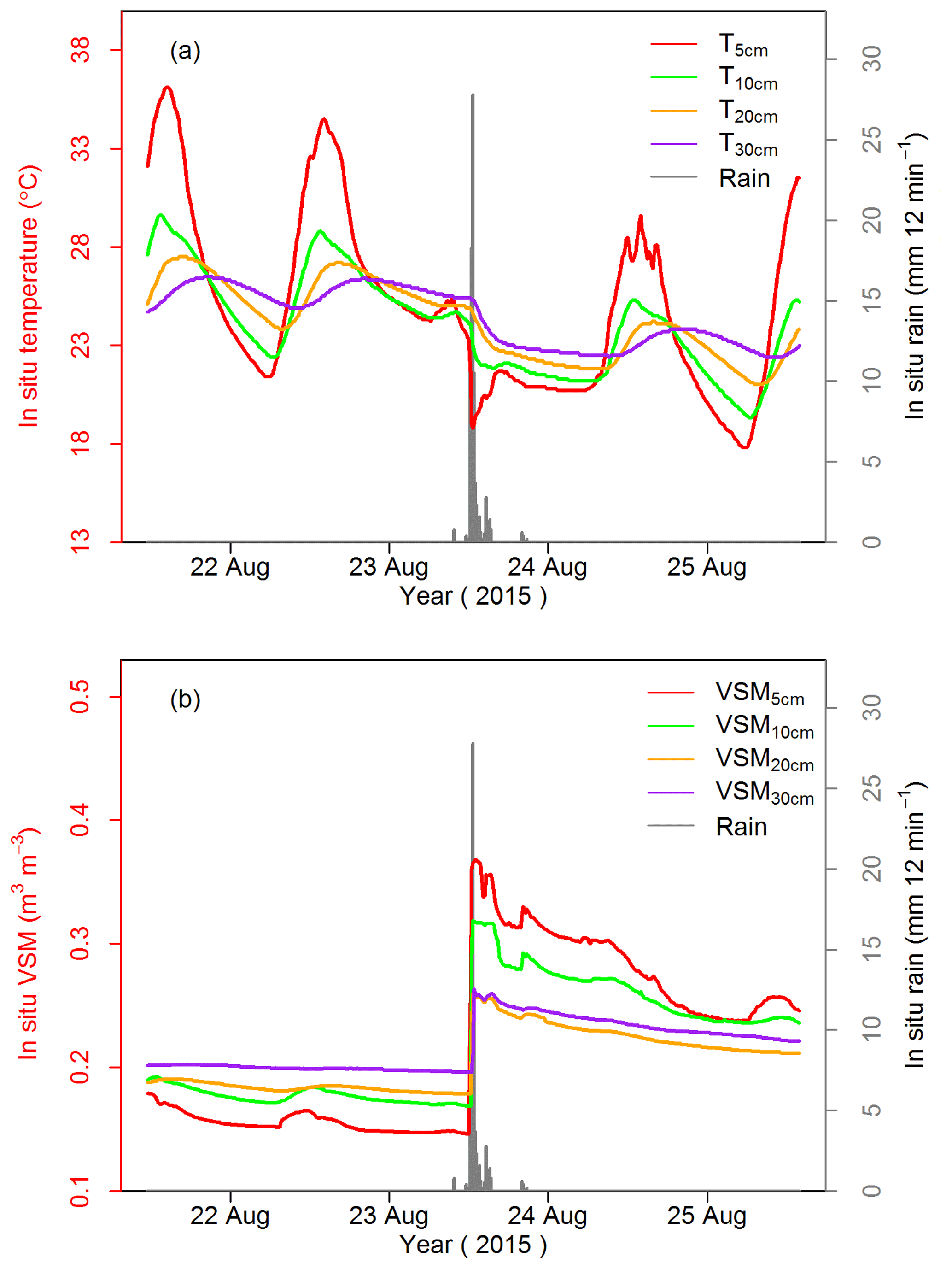
Figure 2In situ soil temperature (a) and soil moisture (b) measured at the PRD station from 21 to 25 August 2015 at depths of 5, 10, 20, and 30 cm, together with the in situ rainfall observations (mm 12 min−1) shown in grey.
The PRD station considered in Fig. 2 is characterized by a Mediterranean climate. The 21 stations of the SMOSMANIA network cover contrasting climate areas (Sect. 2) presenting a different seasonal distribution of precipitation. Figure 3 presents the average monthly rainfall amount across seasons (winter is from December to February) for each SMOSMANIA station over a 9-year period of time, from 2008 to 2016. Differences in the seasonal distribution of precipitation are very large. For the nine westernmost stations (from SBR to SFL) the average monthly rainfall amount across seasons is rather homogenous, although stations under oceanic (O) climate tend to have more precipitation in winter and those under semi-oceanic (SO) climate in spring. For the other 12 stations (from MTM to CBR) under Mediterranean (M) and Mediterranean–mountain (MM) climate conditions, summer is generally drier than other seasons. On the other hand, the autumn is wetter than other seasons, especially in MM climate conditions. The maximum seasonal monthly mean precipitation rate is 272 mm month−1 at the BRN station, and LGC, MZN, and BRZ stations, also under MM climate conditions, present values larger than 150 mm month−1. The differences in rain intensity distribution are analyzed further in Fig. 4 for marked rainfall events (step 3 in Table 2). We can see that both accumulated rainfall and rain duration of individual marked rainfall events can be much larger for M and MM stations than for O and SO stations, especially in the autumn and in winter. The longest rain duration is 41 h in winter, and the maximum accumulated rainfall during a single rainfall event is 370 mm in the autumn, at the same BRN station. On the other hand, most of the marked rainfall events of O and SO stations present less than 50 mm accumulated rainfall and last less than 12 h.

Figure 3Average monthly rainfall (in units of mm) for the 21 SMOSMANIA stations across seasons from 2008 to 2016. Stations are sorted from (left) west to (right) east. Symbols “O”, “SO”, “M”, and “MM” indicate oceanic, semi-oceanic, Mediterranean, and Mediterranean–mountain climates, respectively. Winter season is from December to February.
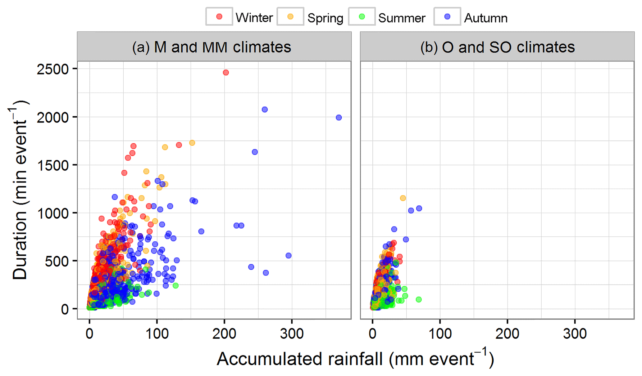
Figure 4Rainfall duration vs. accumulated rainfall across seasons for each marked rainfall event at Mediterranean (M) and Mediterranean–mountain (MM) stations (a) and at oceanic (O) and semi-oceanic (SO) stations (b).
The statistical distribution of δT5 cm (T5 cm increase or decrease in topsoil temperature corresponding to a rainfall event) and the T5 cm change range for marked rainfall events are shown in Fig. 5. In all climate conditions, the topsoil layer is cooler after a marked rainfall event with a probability of 80 %. The δT5 cm difference values are larger than 1 ∘C or smaller than −1 ∘C with a probability of 25 % only. More often than not, a cooling is observed in these conditions rather than a warming. The probability of the T5 cm change range to equal or exceed 1 ∘C is a bit larger: 28 %. This criterion was used to select marked rainfall events affecting T5 cm (step 4 in Table 2). After data sorting, we obtain a total of 1577 events. This corresponds to about eight events per year and per station. Because a lot of marked rainfall events can last several hours, T5 cm change range values ≥1 ∘C can be explained by the diurnal cycle of the surface net radiation rather than the mass movement of rainwater. Since obvious soil-warming rainfall events are not detectable in our observations, we focus on soil-cooling events characterized by a sharp decrease in topsoil temperature (e.g., in Fig. 2) during the 12 min time interval of the soil profile observations. For this purpose, step 5 in Table 2 permits selecting 122 intense soil-cooling rains using minimum ΔT5 cm values ∘C in 12 min. This corresponds to 0.65 events per year and per station.
4.2 Frequency of intense soil-cooling rains
Characteristics of intense soil-cooling rains are summarized in Table 4 and in Fig. S23. Among the 122 identified intense soil-cooling events, 107 occur at stations under M or MM climates and only 15 under the O or SO climates. The spatial and seasonal distribution of these intense soil-cooling rainfall events is shown in Fig. 6 for each station of the SMOSMANIA network. Most of the intense soil-cooling rains (82) are in summer, while only 4 are found in winter. The latter are all for the same BRZ station, under MM climate conditions. In spring and during the autumn, 17 and 19 events are observed, respectively. At six stations, no intense soil-cooling rain is observed in 9 years: three are under O climate conditions (SBR, URG, CRD), two under SO climate conditions (CDM, MNT), and one under MM climate conditions (MZN). The PRD and BRZ stations, under M and MM climate conditions, respectively, present the largest number of events, with a mean rescaled frequency of intense soil-cooling rains of 2.7 per year (Table 1). For the 12 M or MM stations (from MTM to CBR) the mean frequency of intense soil-cooling rains is once a year. More details are shown in Table 1. More characteristics of these 122 intense soil-cooling rains are shown in Fig. 7. These events do not always correspond to a large amount of accumulated rainfall. Actually, about 80 % of these events present accumulated rainfall values smaller than 30 mm. About 80 % of these rains last less than 2 h, and the longest rain duration is less than 5 h. The mean hourly rain rate per event does not exceed 30 mm h−1 for 90 % of the events. This shows that extremely large amounts of rain or large precipitation intensity are not required to produce intense soil cooling. Figure 7 also shows that while 82 % of intense soil-cooling rains present minimum ΔT5 cm values larger than −3 ∘C 12 min−1, very low values (down to −6.5 ∘C 12 min−1) can be observed. During intense soil-cooling rains, the minimum ΔT5 cm contributes to increase the T5 cm change range. For 18 % of the events, the minimum ΔT5 cm represents more than 80 % of the T5 cm change range. For 48 % of the events, the minimum ΔT5 cm represents more than 60 % of the T5 cm change range. The statistical distributions of δT5 cm and δVSM5 cm are also shown in Fig. 7. For intense soil-cooling rains, T5 cm is always lower after the rain than before. The major part (74 %) of the δT5 cm values ranges between −6 and −2 ∘C. For δVSM5 cm, 8 % of the values are slightly negative (the minimum observed δVSM5 cm is −0.006 m3 m−3), and 21 % do not exceed 0.050 m3 m−3. The maximum observed δVSM5 cm is 0.3 m3 m−3.

Figure 5Statistical distributions of δT5 cm (a, b) and T5 cm change range (c, d) during 5714 marked rainfall events for Mediterranean (M) and Mediterranean–mountain (MM) stations (a, c) and for oceanic (O) and semi-oceanic (SO) stations (b, d). The percent value is the ratio of the count of each bin to the total count in all climate conditions. Bin width is 1 ∘C. Bins for values larger than 1 ∘C or smaller than −1 ∘C are in red.
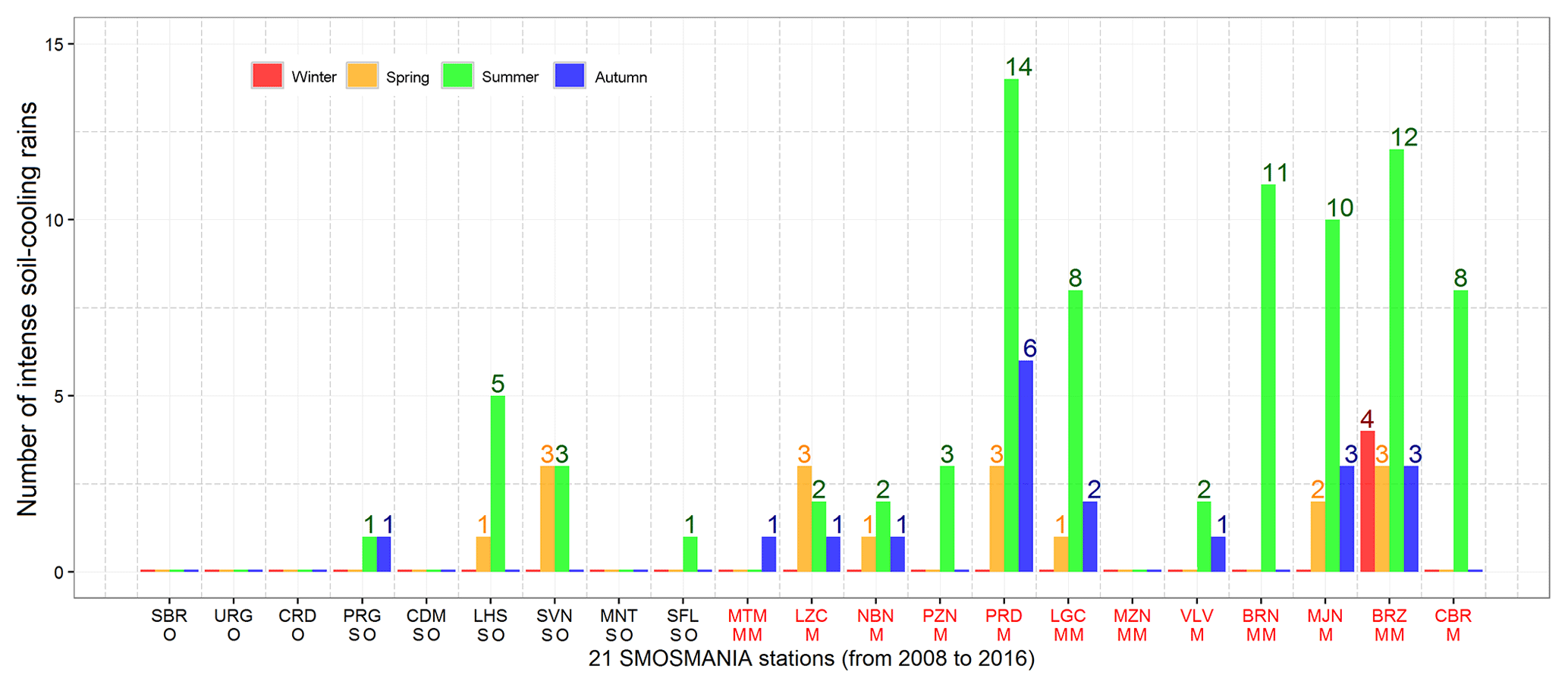
Figure 6Statistical distribution of the 122 intense soil-cooling rains among stations of the SMOSMANIA network across seasons. Red, orange, green, and blue bars are for winter, spring, summer, and the autumn, respectively. Symbols “O”, “SO”, “M”, and “MM” indicate oceanic, semi-oceanic, Mediterranean, and Mediterranean–mountain climates, respectively. Stations are listed from (left) west to (right) east.
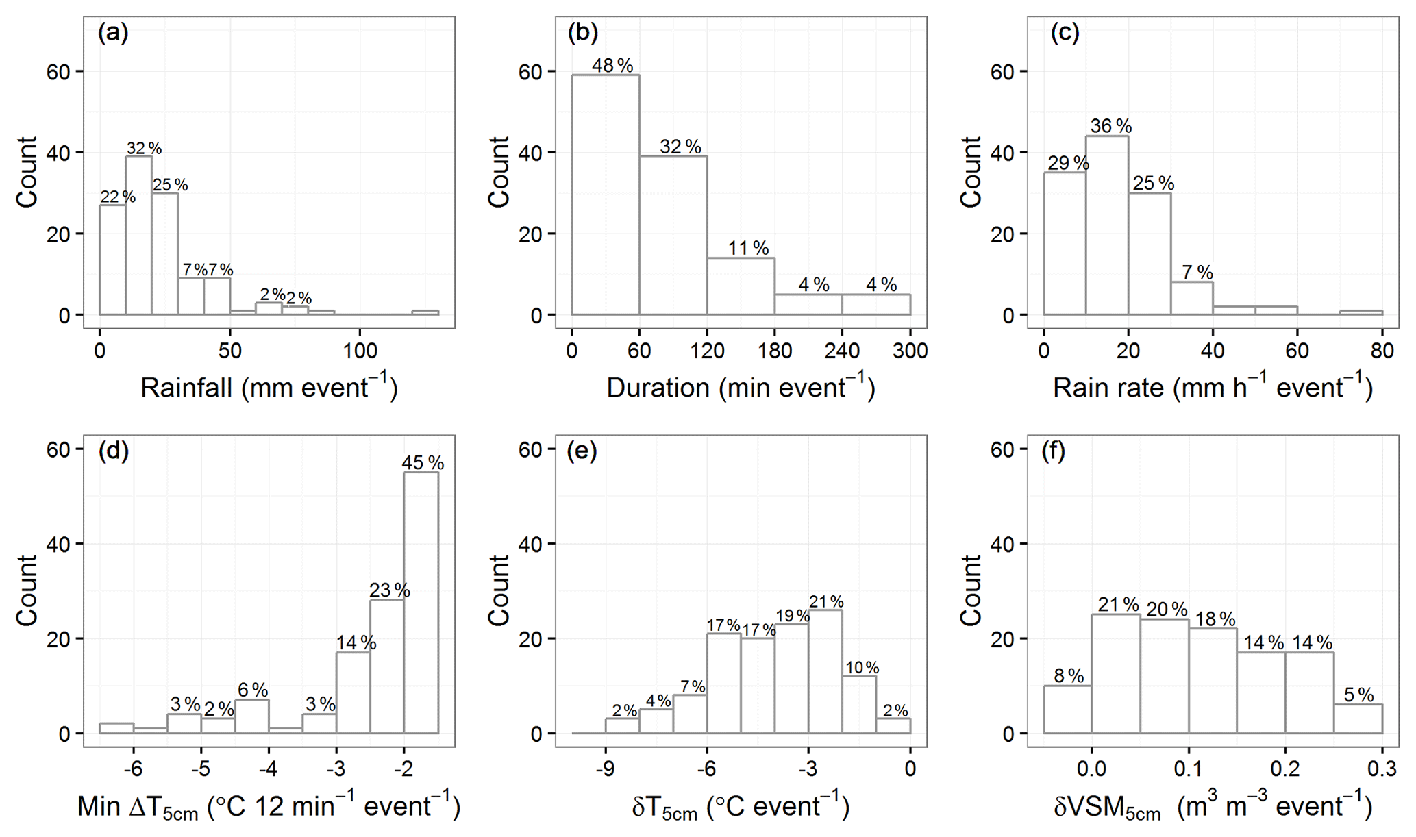
Figure 7Statistical distribution of the 122 intense soil-cooling rains in terms of (Sect. 3.3) accumulated rainfall (a), rain duration (b), rain rate (c), minimum ΔT5 cm (d), δT5 cm (e), and δVSM5 cm (f), with bins of 10 mm, 60 min, 10 mm h−1, 1 ∘C, 1 ∘C, and 0.05 m3 m−3, respectively.
4.3 Estimation of rain temperature from soil temperature and soil moisture observations
Among the 122 intense soil-cooling events, we found 13 cases presenting simultaneous marked changes in T5 cm, VSM5 cm, and VSM10 cm, within a 12 min slot (step 6 in Table 2). Observed values of VSM5 cm, T5 cm, 2 m air temperature Tair at time t1 and t2, and 2 m wet-bulb temperature Twb at time t1 for these 13 example rains are listed in Table 5, together with the accumulated precipitation of the considered rainfall events and the peak rainfall intensity (mm 12 min−1) of each rain. Among these 13 cases, 2 are under SO climate conditions (PRG and SFL) and 11 are under M and MM climate conditions (from LZC to CBR in Table 5). The latter include five cases from the same station, PRD. From a seasonal perspective, 2 cases occurred in spring (cases 9 and 12), 1 during the autumn (case 3), and the other 10 cases occurred in summer.
Table 5The estimated rain temperatures (Train) for 13 intense soil-cooling events, together with the in situ observations of VSM5 cm, T5 cm, Tair at time t1 and t2, and Twb at time t1. The time lapse from time t1 to t2 is 12 min. For rain events 9 and 12, Eq. (4) is used to estimate the amount of melting hail at the soil surface. Train values lower by −5 ∘C than Tair at time t1 are in bold. Stations are listed from west (top) to east (bottom).
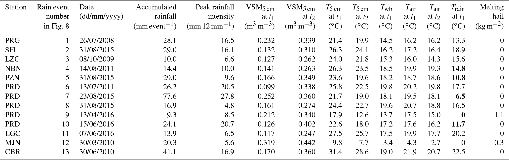
Table 5 also shows the rain temperature estimates at time t1 (Train) derived from Eq. (3) and the amount of melted hail derived from Eq. (4). Interestingly, the only two cases occurring in spring (cases 9 and 12) correspond to melting hail events. Taking the PRD station case 9 as an example, the measured precipitation amount is 9.3 kg m−2 during a rainfall event of 36 min, with an average rain rate of 15.5 mm h−1. From time t1 to t2, the T5 cm topsoil temperature decreases very fast from 17.9 to 12.6 ∘C (−5.3 ∘C in 12 min), and the air temperature also decreases from 17.5 to 15.0 ∘C (−2.5 ∘C in 12 min). During the same time lapse, VSM5 cm increases by +0.13 m3 m−3. Storms with hail were reported in the press and in social media at many places of southern France on 23 April 2016, including close to the PRD region (Infoclimat, 2016). Using Eq. (4), one can estimate the amount of water originating from melting hail: about 1 kg m−2. Soil temperature and soil moisture time series for all these 13 rain examples are shown in Figs. S3–S15. Thunderstorms and hail were also reported for case 12 (Infoclimat, 2010).
Figure 8 shows the estimated Train vs. Tair and T5 cm at time t1. While most of the Tair values range between 16 and 22 ∘C, except for case 12 (Tair=4.3 ∘C), the estimated Train values present a larger variability, from 0 to 22.5 ∘C. Excluding the two spring cases (9 and 12), the standard deviation of Train values in Table 5 is 4.6 ∘C, which is much larger than for Tair, 1.9 ∘C.
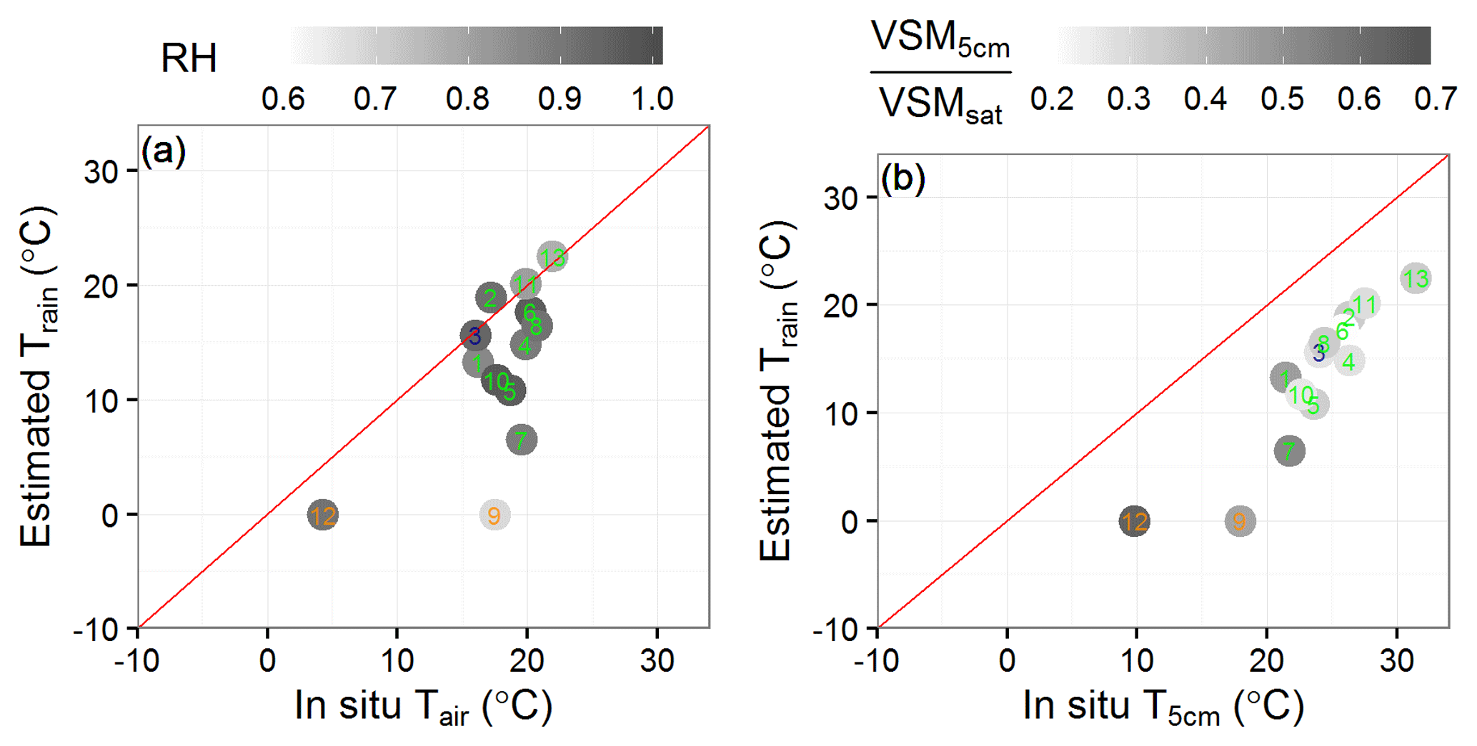
Figure 8Estimated Train for the 13 cases listed in Table 5 vs. observed ambient Tair (a) and observed T5 cm (b), with levels of grey indicating air relative humidity (RH, dimensionless) and VSM5 cm to VSMsat ratio (dimensionless) values at time t1.
For the 13 storms listed in Table 5, Train (T5 cm) tends to be lower (higher) than Tair, with a mean difference of −5.1 ∘C (+6.0 ∘C). On average, Train is cooler than topsoil by −11.1 ∘C. Train is cooler than Twb by −3.8 ∘C. For cases 2, 11, and 13, Train is close to Tair. For cases 1 and 3, Train is close to Twb. The other cases present Train values much cooler than Tair and Twb. In particular, Train is cooler than Tair by more than 5 ∘C for five cases (4, 5, 7, 9, 10), among which three cases (7, 9, 10) occurred at the PRD station. At time t1, RH ranges from 68 % to 97 % and ranges from 20.7 % to 63.8 %. Soil-cooling rate ΔT5 cm values range from −5.3 to −1.5 ∘C in 12 min. The corresponding air cooling values are less pronounced, ranging from −2.5 to 0.0 ∘C. For case 9, increases only by 27 % during the considered 12 min slot. This is a relative small increase compared to other cases, which is less than the median value of 29 % and much less than the maximum value of 58 % observed for case 10 at the same station. Despite the moderate soil wetting in case 9, T5 cm values presented the most pronounced decrease (−5.3 ∘C). The T5 cm value at time t2 also presented the largest difference with the estimated rain temperature (+12.6 ∘C).
5.1 How accurate are rain temperature estimates?
In this study, an attempt is made to estimate rain temperature using observations in the topsoil layer.
In Eqs. (2) and (3), it is assumed that the precipitation-induced sensible heat flux dominates heat exchanges in the topsoil layer. Since soil properties are known, the mean PH value can be estimated from Eq. (2) for the intense soil-cooling events used to retrieve Train (see Table 5). For the 10 events of Table 5 occurring at summertime, this flux ranges from 408 to 1009 W m−2, with a mean value of 648 W m−2. These PH flux values are very high and represent large fractions of absolute values of the net radiation Rnet (i.e., the amount of energy available for surface heat exchanges, driven by the incoming solar radiation, that could be simulated without accounting for PH). They are probably often much larger than Rnet because the Rnet energy budget component is generally small during rainfall events, in relation to the low incoming solar radiation. Moreover, 7 events out of 10 occur at nighttime or at dusk (see Supplement), i.e., in small Rnet value conditions. The Rnet variable is not measured at SMOSMANIA stations. Typical measured summertime values of the maximum daily Rnet over the grassland site of Meteopole-Flux in southwestern France (Zhang et al., 2018) range from about 200 W m−2 during cloudy rainy days to about 700 W m−2 in clear sky conditions. At nighttime, absolute Rnet values rarely exceed 100 W m−2.
Because Eqs. (3) and (4) include soil heat capacity (Eq. 1), the static soil properties must be known together with the time-evolving VSM and soil temperature. In particular, the volumetric fraction of gravels is the most variable static soil characteristic in Table 3: fgravel ranges from 0 to 0.41 m3 m−3 at CRD and BRN stations, respectively. Among stations of the 13 rain retrieval cases in Table 5, fgravel ranges from 0.05 to 0.34 m3 m−3 at PZN and PRD, respectively. The fraction of gravels was not measured at a depth of −5 cm. Instead, values given in Table 3 are derived from gravimetric measurements made at −10 cm. In order to assess to what extent uncertainties on fmin values may affect the retrieved Train values, two numerical experiments (Exp1 and Exp2) were made using other soil characteristics than those listed in Table 3 (control experiment):
-
Exp1 used the reassembled static soil volumetric fractions of soil minerals and SOM at a depth of 5 cm assuming fgravel=0 m3 m−3. This was equivalent to considering fine earth only, and the resulting fSOM and fmin fractions were larger and smaller than in the control experiment, respectively. This tended to increase (Eq. 1) and to decrease Train (Eq. 3).
-
Exp2 used the measured soil characteristics at a depth of 10 cm (Calvet et al., 2016). The impact of Exp2 on fSOM, fmin, , and Train varied a lot from one station to another.
Volumetric fractions of the topsoil elements used in Exp1 and Exp2 are listed in Tables S2 and S3, respectively. Differences in fSOM and fmin values are listed in Table 6.
Table 6The estimated Train differences, fmin differences, and fSOM differences between Exp1 and control and between Exp2 and control. Changes in values of Train larger than ±0.5 ∘C are in bold. Changes in values of volumetric fractions larger than 0.05 m3 m−3 are in bold.
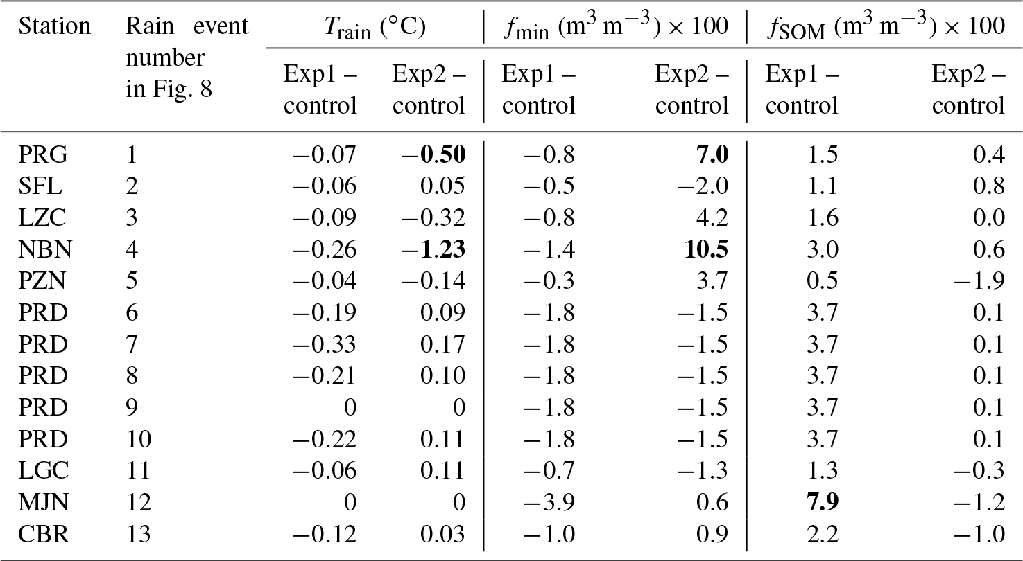
Differences in estimated Train values for Exp1 and Exp2 with respect to the control are shown in Table 6. In Exp1, Train estimates tend to present slightly lower values, with differences down to −0.3 ∘C, and the median difference value is −0.1 ∘C, with a standard deviation of 0.1 ∘C. In Exp2, Train differences range from −1.23 to +0.17 ∘C, and the median difference value is 0 ∘C, with a standard deviation of 0.4 ∘C. Merging results from Exp1 and Exp2, 80 % of the statistical distribution of Train differences range between −0.3 and +0.1 ∘C. The most marked changes in Train (−0.50 and −1.23 ∘C) are observed for Exp2 (cases 1 and 4, at PRG and NBN stations, respectively). They correspond to the largest changes in fmin (+0.070 and +0.105, respectively). This gives an idea of the uncertainties on Train related to poorly known soil heterogeneities and to their impact on the soil characteristics measured in the field.
Another source of uncertainties is that the topsoil layer, from the soil surface down to a depth of −0.1 m, may not be completely affected by the rainfall event or that the instruments positioned at a depth of −5 cm may not be able to sample mean values relevant for the topsoil layer. In order to limit this effect, we selected only 13 intense soil-cooling events by imposing a marked change in VSM10 cm during the considered 12 min slot. If the latter condition is ignored, 32 soil-cooling events can be considered instead of 13, and we checked that similar results are found (not shown).
A limitation of the method used in this study is that the soil moisture and soil temperature probes at a depth of 5 cm are not placed at exactly the same location. We found some examples for which the VSM response to rain does not match with the drop in topsoil temperature (Figs. S18, S19, S20, S21, and S22). This limited the number of events for which rainwater temperature could be estimated.
More research is needed to develop techniques to measure rainwater temperature. Instruments similar to the rain temperature equipment of Byers et al. (1949) could be developed. Our results show that using automatic temperature and volumetric moisture observations in a porous medium of known thermal properties has potential to estimate Train and possibly the amount of hailstones in real time.
5.2 Does soil cooling matter?
We showed (e.g., Fig. 2) that the temperature of raindrops reaching the soil surface can impact the soil temperature profile during several hours. Investigating the impact on longer time periods would require using a LSM able to activate or deactivate the representation of sensible heat input from liquid water into the soil. This impact was investigated experimentally by Wierenga et al. (1975) through an irrigation experiment with cold and warm water (4.1 and 21.6 ∘C, respectively). They showed that 42 h was needed before differences in soil temperature at a depth of 0.2 m were reduced to less than 1 ∘C, and more than 5 d was needed below a depth of 0.5 m. They used quite large irrigation amounts of more than 120 mm. Figure 7 shows that accumulated rainfall during one event can exceed 120 mm in Mediterranean climate conditions (M and MM). Such events are not observed in O and SO conditions, but less intense precipitation events can impact the surface energy budget, even if this is not obvious in the soil temperature time series. Figure 7 shows that intense soil-cooling events (step 5 in Table 2) are associated with rather uniformly distributed increases in topsoil VSM values. Actually, the statistical distribution of δVSM5 cm values tends to shift towards larger values at each data-sorting step listed in Table 2. This is illustrated by Fig. 9 for steps 2, 3, and 4. For fully documented rainfall events (step 2), VSM5 cm does not increase for about 60 % of the rainfall events (δVSM5 cm≤0 m3 m−3 12 min−1). Two possible reasons are that (1) rainwater can be intercepted by vegetation and/or litter, especially when the rain is very slight and/or the soil ground is very dry; and (2) VSM5 cm is close to saturation, so no VSM5 cm increase is observed. We found examples under the above two situations, shown in Fig. S16 (VSM5 cm is relatively small and the rainwater might be intercepted) and Fig. S17 (VSM5 cm is close to saturation). For steps 3 and 4, Fig. 9 shows that only 7 % to 9 % of VSM5 cm values do not increase. About the same proportion is observed for the 122 intense soil-cooling rains (Fig. 7).

Figure 9Statistical distribution of δVSM5 cm for 104 178 fully documented rainfall events (a), 5714 marked rainfall events (b), and 1577 marked rainfall events affecting topsoil temperature (c) defined in Table 2.
Assessing the impact of neglecting precipitation-induced sensible heat in the soil temperature simulations of a LSM is a key issue. Developing LSMs able to represent the sensible heat input from liquid water into the soil is needed, as well as a way to diagnose rainwater temperature from atmospheric model simulations (Feiccabrino et al., 2015). Soil temperature and soil moisture simulations from the ISBA LSM are presented in the Supplement (Figs. S24 and S25). It is shown that ISBA simulations are not able to represent the response of soil variables to intense soil-cooling precipitation events. Now, the ISBA model has no representation of heat exchanges due to water mass movement. This process needs to be introduced in ISBA. We think that data from a fully instrumented site including direct measurements of rain water temperature are needed to completely address this issue and to validate the upgraded model version. Such an experiment would give insights to understand when, where, and why soil cooling occurs or not and would be valuable to help model development. In particular, the precipitation-induced sensible heat flux is not limited to intense precipitation, and the impact of this process on the surface energy budget needs to be investigated in all conditions.
Attempts were made in a few studies to simulate the precipitation-induced sensible heat (e.g., Emanuel et al., 2008; Wang et al., 2016), but, in general, it was assumed that Train was equal to Twb. This study shows that Train can be much lower than Twb during severe convective events and confirms the findings of Byers et al. (1949). Since severe convective events associated with the intense soil-cooling events observed in this study tend to become more and more frequent in relation to climate change (Feng et al., 2016), soil-cooling effects may play a role in the response of the Earth system to climate change. Moreover, rainwater temperature estimates from observation networks or from atmospheric model simulations could be beneficial for a number of applications such as urban heat island monitoring (e.g., Jelinkova et al., 2015), drinking water quality monitoring (e.g., Chubaka et al., 2018), the estimation of the emission rates of greenhouse gases by soils (e.g., Gagnon et al., 2018), or the quantification of soil erosion (e.g., Sachs and Sarah, 2017).
In situ rain temperature measurements are rare. We used the soil moisture and soil temperature observations from the SMOSMANIA network over 9 years in southern France to assess the cooling effects on soils of rainfall events. The rainwater temperature was estimated using observed changes in topsoil volumetric soil moisture and soil temperature in response to the rainfall event. We found that most (72 %) marked rainfall events did not impact the T5 cm change range more than ±1 ∘C. On the other hand, about 2 % of marked rainfall events triggered intense soil cooling with drops in T5 cm ( ∘C in 12 min. Such intense soil-cooling rains were mainly observed under Mediterranean climate conditions, in summer, at daytime. The average frequency of the occurrence of such events for the 12 Mediterranean stations was once a year. Among all these intense soil-cooling rains, the minimum observed value of ΔT5 cm was −6.5 ∘C in 12 min. Rain temperature estimates were obtained for 13 cases. They were generally lower than the ambient air temperatures, wet-bulb temperatures, and T5 cm values (with mean differences of −5.1, −3.8, and −11.1 ∘C, respectively). In five cases, rain temperature estimates were much cooler than air temperature, by at least −5 and down to −17.5 ∘C, likely in relation to hailstones melting just before reaching the surface or melting at the surface of the soil. More research is needed to develop measurement techniques for rainwater temperature and perform such measurements in contrasting climate conditions.
The soil moisture (temperature) observations are available to the research community through the International Soil Moisture Network website (https://ismn.geo.tuwien.ac.at/, ISMN, 2018).
| T5 cm (∘C) | in situ soil temperature at a depth of 5 cm |
| ΔT5 cm (∘C 12 min−1) | T5 cm change every 12 min during a rainfall event |
| T5 cm change range (∘C) | maximum minus minimum T5 cm during a rainfall event, including 12 min slots just after and before the rainfall event |
| δT5 cm (∘C) | T5 cm just after the rainfall event minus T5 cm just before the rainfall event |
| VSM5 cm (m3 m−3) | in situ volumetric soil moisture (VSM) at a depth of 5 cm |
| ΔVSM5 cm (m3 m−3 12 min−1) | VSM5 cm change every 12 min during a rainfall event |
| VSM5 cm change range (m3 m−3) | maximum minus minimum VSM5 cm during a rainfall event, including 12 min slots just after and before the rainfall event |
| δVSM5 cm (m3 m−3) | VSM5 cm just after the rainfall event minus VSM5 cm just before the rainfall event |
| Δz (m) | depth of the topsoil layer (0.1 m in this study) |
| TISBA (∘C) | ISBA soil temperature simulations at a depth of 5 cm |
| ΔTISBA (∘C 12 min−1) | TISBA change every 12 min during a rainfall event |
| Tair (∘C) | observed ambient air temperature at 2 m |
| Twb (∘C) | ambient wet-bulb temperature at 2 m calculated using the Stull (2011) equation |
| Train (∘C) | estimated rain temperature |
| PH (W m−2) | precipitation-induced sensible heat flux |
| Rnet (W m−2) | net radiation flux |
| RH (dimensionless) | in situ air relative humidity at 2 m |
| VSMsat (m3 m−3) | VSM at saturation (i.e., the soil porosity) |
| (dimensionless) | VSM5 cm to VSMsat ratio or degree of saturation |
| SOM | soil organic matter |
| fclay, fgravel, fmin, fsand, fsilt, fSOM (m3 m−3) | volumetric fractions of clay, gravels, soil minerals, sand, silt, and SOM |
| , Cwater, Cmin, CSOM (J m−3 K−1) | heat capacity values of the topsoil layer at time t, water, soil minerals, and SOM |
| O, SO, M, MM | oceanic, semi-oceanic, Mediterranean, Mediterranean–mountain climate conditions |
| For the first eight symbols, the subscript “5 cm” stands for observations made at a depth of 5 cm. | |
| In Table 2, marked rainfall events affecting T5 cm are defined with T5 cm change range ≥1 ∘C. Intense soil cooling during | |
| a marked rainfall event is defined with minimum ∘C in 12 min. | |
| In Table 1, the rescaled number of intense soil-cooling events is calculated as | |
| , | |
| where Ns is the number of intense soil-cooling events for one season at one station, and fs is the proportion of missing | |
| data for the same season at the same station (see Table S1 and Fig. S2 in the Supplement). The fs values for each season | |
| are estimated using the total missing data proportion for all seasons and the scaled seasonal distribution of the fraction | |
| of missing data. | |
The supplement related to this article is available online at: https://doi.org/10.5194/acp-19-5005-2019-supplement.
SZ and JCC performed the conceptualization; SZ and CM performed the data processing; SZ, JCC, and CM performed the result analysis; SZ wrote the original draft; SZ, JCC, and CM reviewed and edited the paper.
The authors declare that they have no conflict of interest.
This article is part of the special issue “Hydrological cycle in the Mediterranean (ACP/AMT/GMD/HESS/NHESS/OS inter-journal SI)”. It is not associated with a conference.
This work is a contribution to the HyMeX program (https://www.hymex.org/, last access: April 2019). We thank our Météo-France colleagues for their support in collecting, checking, and archiving the SMOSMANIA data: Annick Auffray, Catherine Bienaimé, Marc Bailleul, Basile Baumann, Laurent Brunier, Jérôme Candiago, Anne Chaumont, Jacques Couzinier, Mathieu Créau, Pierre Farges, Hélène Fillancq, Noureddine Fritz, Philippe Gillodes, Sandrine Girres, Michel Gouverneur, Didier Grimal, Viviane Isler, Maryvonne Kerdoncuff, Matthieu Lacan, Pierre Lantuejoul, Franck Lavie, William Maurel, Roland Mazurie, Nicolas Naudet, Dominique Paulais, Bruno Piguet, Fabienne Simon, Dominique Simonpietri, Marie-Hélène Théron, and Marie Yardin.
This paper was edited by Domenico Cimini and reviewed by three anonymous referees.
Byers, H. R., Moses, H., and Harney, P. J.: Measurement of rain temperature, J. Meteorol., 6, 51–55, https://doi.org/10.1175/1520-0469(1949)006<0051:MORT>2.0.CO;2, 1949.
Calvet, J. C., Fritz, N., Froissard, F., Suquia, D., Petitpa, A., and Piguet, B.: July. In situ soil moisture observations for the CAL/VAL of SMOS: the SMOSMANIA network, In Geoscience and Remote Sensing Symposium, IGARSS, Barcelona, Spain, 23–28 July 2007, 1196–1199, https://doi.org/10.1109/IGARSS.2007.4423019, 2007.
Calvet, J.-C., Fritz, N., Berne, C., Piguet, B., Maurel, W., and Meurey, C.: Deriving pedotransfer functions for soil quartz fraction in southern France from reverse modeling, SOIL, 2, 615–629, https://doi.org/10.5194/soil-2-615-2016, 2016.
Chubaka, C. E., Whiley, H., Edwards, J. W., and Ross, K. E.: Microbiological values of rainwater harvested in Adelaide, Pathogens, 7, 21, https://doi.org/10.3390/pathogens7010021, 2018.
Decharme, B., Martin, E., and Faroux, S.: Reconciling soil thermal and hydrological lower boundary conditions in land surface models, J. Geophys. Res.-Atmos., 118, 7819–7834, https://doi.org/10.1002/jgrd.50631, 2013.
Emanuel, K., Callaghan, J., and Otto, P.: A hypothesis for the redevelopment of warm-core cyclones over northern Australia, Mon. Weather Rev., 136, 3863–3872, https://doi.org/10.1175/2008MWR2409.s1, 2008.
Feiccabrino, J., Graff, W., Lundberg, A., Sandström, N., and Gustafsson, D.: Meteorological knowledge useful for the improvement of snow rain separation is surface based models, Hydrology, 2, 266–288, https://doi.org/10.3390/hydrology2040266, 2015.
Feng, Z., Leung L. R., Hagos, S., Houze, R. A., Burleyson, C. D., and Balaguru, K.: More frequent intense and long-lived storms dominate the springtime trend in central US rainfall, Nat. Commun., 7, 13429, https://doi.org/10.1038/ncomms13429, 2016.
Gagnon, S., Allard, M., and Nicosia, A.: Diurnal and seasonal variations of tundra CO2 emissions in a polygonal peatland near Salluit, Nunavik, Canada, Arctic Science 4, 1–15, https://doi.org/10.1139/as-2016-0045, 2018.
Houpeurt, A., Delouvrier, J., and Iffly, R.: Fonctionnement d'un doublet hydraulique de refroidissement, La Houille Blanche, 3, 239–246, available at: https://www.shf-lhb.org/fr/articles/lhb/pdf/1965/03/lhb1965020.pdf (last access: August 2018), 1965.
Infoclimat: Bilan météo du mardi 20 mars 2010, available at: https://www.infoclimat.fr/actualites/bqs/11100/bilan-meteo-du-mardi-30-mars-2010.html, (last access: August 2018), 2010.
Infoclimat: Website forum, Suivi du temps dans les regions Méditerranéennes (13 avril 2016), available at: https://forums.infoclimat.fr/f/topic/349-suivi-du-temps-dans-les-r%C3 %A9 gions-m%C3 %A9 diterran%C3 %A9 ennes/?page=10, (last access: August 2018), 2016.
ISMN: International Soil Moisture Network, available at: https://ismn.geo.tuwien.ac.at/, (last access: August 2018), 2018.
Jelinkova, V., Dohnal, M., and Picek, T.: A green roof segment for monitoring the hydrological and thermal behavior of anthropogenic soil systems, Soil Water Res., 10, 262–270, https://doi.org/10.17221/17/2015-SWR, 2015.
Kinzer, G. D. and Gunn, R.: The evaporation, temperature and thermal relaxation-time of freely falling waterdrops, J. Meteorol., 8, 71–83, https://doi.org/10.1175/1520-0469(1951)008<0071:TETATR>2.0.CO;2, 1951.
Kollet, S. J., Cvjanovic, I., Schüttemeyer, D., Maxwell, R. M., Moene, A. F., and Bayer, P.: The influence of rain sensible heat and subsurface energy transport on the energy balance at the land surface, Vadose Zone J., 8, 846–857, https://doi.org/10.2136/vzj2009.0005, 2009.
Ruti, P. M., Somot, S., Giorgi, F., Dubois, C., Flaounas, E., Obermann, A., Dell'Aquila, A., Pisacane, G., Harzallah, A., Lombardi, E., Ahrens, B., Akhtar, N., Alias, A., Arsouze, T., Aznar, R., Bastin, S., Bartholy, J., Béranger, K., Beuvier, J., Bouffies-Cloché, S., Brauch, J., Cabos, W., Calmanti, S., Calvet, J.-C., Carillo, A., Conte, D., Coppola, E., Djurdjevic, V., Drobinski, P., Elizalde-Arellano, A., Gaertner, M., Galàn, P., Gallardo, C., Gualdi, S., Goncalves, M., Jorba, O., Jordà, G., L'Heveder, B., Lebeaupin-Brossier, C., Li, L., Liguori, G., Lionello, P., Maciàs, D., Nabat, P., Onol, B., Rajkovic, B., Ramage, K., Sevault, F., Sannino, G., Struglia, M. V., Sanna, A., Torma, C., and Vervatis, V.: MED-CORDEX initiative for Mediterranean Climate studies, B. Am. Meteorol. Soc., 97, 1187–1208, https://doi.org/10.1175/BAMS-D-14-00176.1, 2016.
Sachs, E. and Sarah, P.: Combined effect of rain temperature and antecedent soil moisture on runoff and erosion on Loess, Catena, 158, 213–218, https://doi.org/10.1016/j.catena.2017.07.007, 2017.
Stull, R.: Wet-bulb temperature from relative humidity and air temperature, J. Appl. Meteorol. Clim., 50, 2267–2269, https://doi.org/10.1175/JAMC-D-11-0143.1, 2011.
Wang, F., Cheruy, F., and Dufresne, J.-L.: The improvement of soil thermodynamics and its effects on land surface meteorology in the IPSL climate model, Geosci. Model Dev., 9, 363–381, https://doi.org/10.5194/gmd-9-363-2016, 2016.
Wei, N., Dai, Y., Zhang, M., Zhou, L., Ji, D., Zhu, S., and Wang, L.: Impact of precipitation-induced sensible heat on the simulation of land-surface air temperature, J. Adv. Model. Earth Sy., 6, 1311–1320, https://doi.org/10.1002/2014MS000322, 2014.
Wierenga, P. J., Hagan, R. M., and Nielsen, D. R.: Soil temperature profiles during infiltration and redistribution of cool and warm irrigation water, Water Resour. Res., 6, 230–238, 1975.
Zhang, S., Calvet, J.-C., Darrozes, J., Roussel, N., Frappart, F., and Bouhours, G.: Deriving surface soil moisture from reflected GNSS signal observations from a grassland site in southwestern France, Hydrol. Earth Syst. Sci., 22, 1931–1946, https://doi.org/10.5194/hess-22-1931-2018, 2018.