2.1 Airborne data collection

Aircraft data were collected by a Mooney Bravo and Mooney Ovation, which are fixed-wing single-engine airplanes operated by Scientific Aviation, Inc. The wings are modified to sample air through inlets, which flow to the onboard analyzers. Temperature and relative humidity data were collected by a Visalia HMP60 humidity and temperature probe, ozone was measured with a dual-beam ozone absorption monitor (2B Technologies, model 205), and NO was measured by chemiluminescence (ECO PHYSICS, model CLD 88). NO_x was measured by utilizing a photolytic converter (model 42i BLC2-395 manufactured by Air Quality Design, Inc.). For flights performed in 2016, a pre-reaction chamber was also installed to monitor and subtract the changing background signal, reducing the detection threshold to <50 ppt. Frequent calibrations were performed in the field, generally once per deployment, with zero and span checks daily. Calibrations for NO measurements were performed with a NIST-traceable standard by Scott-Marrin, Inc. Calibrations for NO_x measurements were performed by titrating the NO standard with an ozone generator (2B Technologies, model 206 Ozone Calibration Source.) During routine operation on the aircraft, the lamp of the photolytic converter was toggled on and off at 20 s intervals during the flights (corresponding to approximately 1.5 km horizontal and 50 m vertical displacements by the aircraft), requiring linear interpolation for continuous NO and NO₂ data. The pre-reaction chamber was toggled on for a 40 s period every 10 min in order to measure the background signals of NO and NO_x, and the background signals were subtracted from the measurement. The interpolated NO₂ signal was noted to decay approximately exponentially after powering up, which sometimes affected the first 15–30 min of flight. The presumed artifact was successfully replicated in the laboratory with a constant NO₂ concentration and was removed by exponential detrending.

Winds are measured using a dual-hemisphere global positioning system combined with direct airspeed measurements, as described in Conley et al. (2014). The winds are measured at 1 Hz, and the power spectra are observed to fit the Kolmogorov scaling law within the inertial subrange (approximately 0.12–0.5 Hz in the daytime convective boundary layer corresponding to roughly 150–600 m spatial scales). At night, the $-\mathrm{5}/\mathrm{3}$ slope is observed from 0.02 to 0.5 Hz (Fig. 1), corresponding to length scales of 150–3700 m, the largest of which are likely contributions from buoyancy waves. This is evident by the calculated Brunt–Väisälä frequencies (Fig. 2), which have an average value of 0.023 Hz in the NBL. For simplicity's sake, we consider anything smaller than this buoyancy frequency to be “turbulence” and use $\mathrm{1}/N_{\mathrm{BV}}\sim \mathrm{50}$ s as the sampling time to observe wind variances, though we recognize that this cutoff is somewhat arbitrary. The TKE is estimated by correcting the observed wind variance of a given detrended 50 s signal with the integrated nocturnal power spectra beyond the Nyquist frequency (0.5 Hz) using a $-\mathrm{5}/\mathrm{3}$ extrapolation, which indicates that approximately 11 % of the total variance is not directly captured by the system. Only horizontal winds are measured, and thus similarity assumptions are required to estimate vertical wind variance (${\mathit{\sigma }}_{\mathrm{w}}^{\mathrm{2}})$. While some similarity relationships have been reported for the NBL (Nieuwstadt, 1984), we were not able to measure the governing parameters. However, Banta et al. (2006) reported a meta-analysis of NBL studies with an average ${\mathit{\sigma }}_{\mathrm{w}}^{\mathrm{2}}/{\mathit{\sigma }}_{\mathrm{u}}^{\mathrm{2}}$ of 0.39, where ${\mathit{\sigma }}_{\mathrm{u}}^{\mathrm{2}}$ is the streamwise variance. We applied this correction to our TKE measurements to account for the missing vertical wind variance.

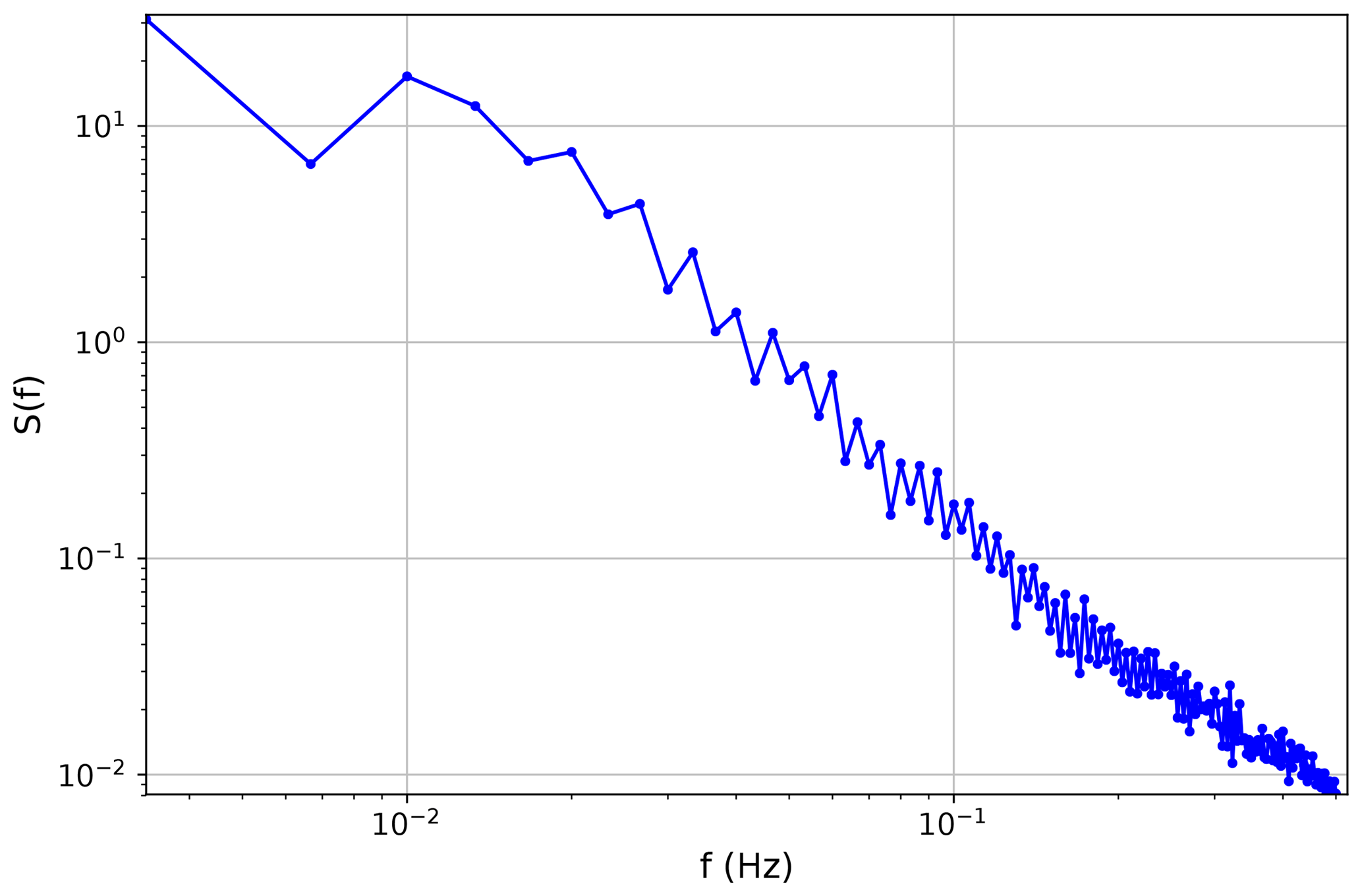
Figure 1Power spectra for nighttime winds averaged over 309 5 min samples. The average airspeed was 76.6 m s⁻¹.

Download

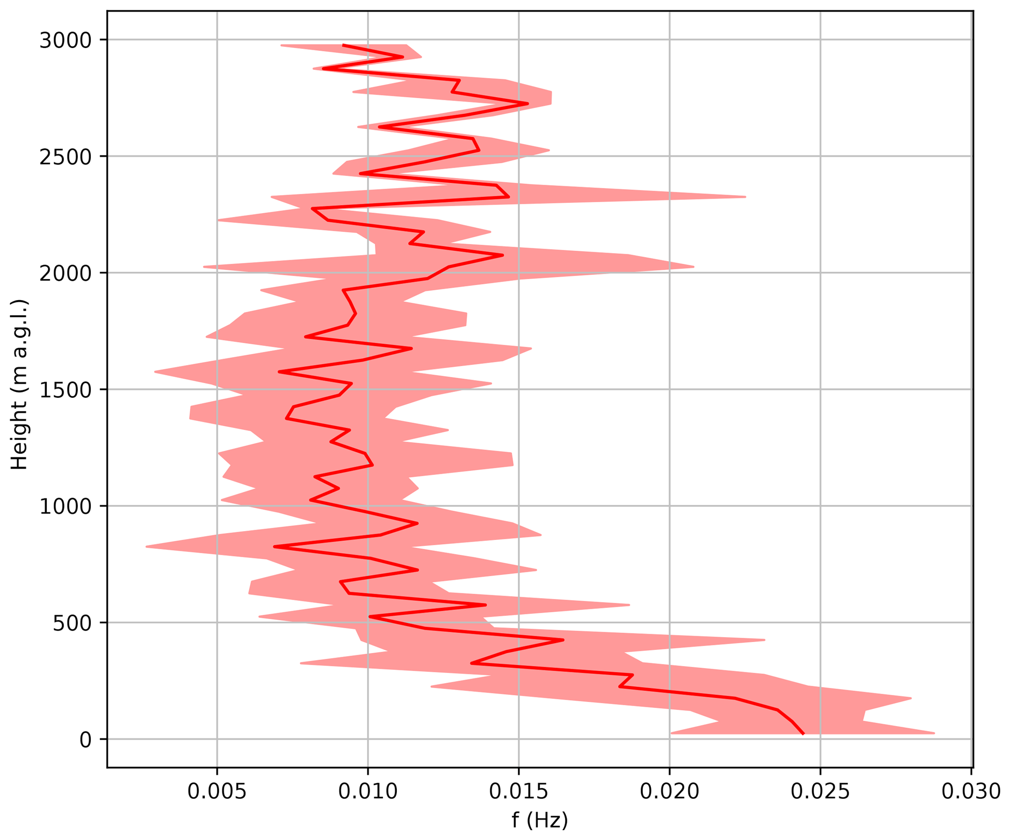
Figure 2Mean and standard deviation profile of Brunt–Väisälä frequencies for all late-night flights. The mean value within the stable boundary layers is 0.023 s⁻¹.

Download

Data were collected on five separate deployments (10–12 September 2015, 2–4 June 2016, 28–29 June 2016, 24–26 July 2016, 12–18 August 2016). During a given deployment, four flights per day were conducted (07:00, 11:00, 15:00, and 22:00 PST). Each deployment consisted of stationing the airplane at Fresno Yosemite International Airport (FAT), with each flight comprising a transect to Bakersfield Meadows Field Airport (BFL) and back, spanning approximately 2 h and 15 min (Fig. 3). Profiles of the full boundary layer and above were taken at Fresno and Bakersfield. Along the Fresno–Bakersfield transect, altitude legs of 500, 1000, and 1500 m a.g.l. were conducted in a randomized order. Low passes were also flown over the Tulare (TLR), Delano (DLO), and Bakersfield airports, but in 2016 we replaced the low approaches at Tulare with Visalia (VIS) to coincide with the NOAA lidar deployment. All of these airports are within a few hundred meters of California Highway 99, or in the case of Fresno and Bakersfield within an urban center. If time permitted on any given flight, we typically completed an extra profile at Visalia or flew west toward Hanson to better sample the nocturnal LLJ.

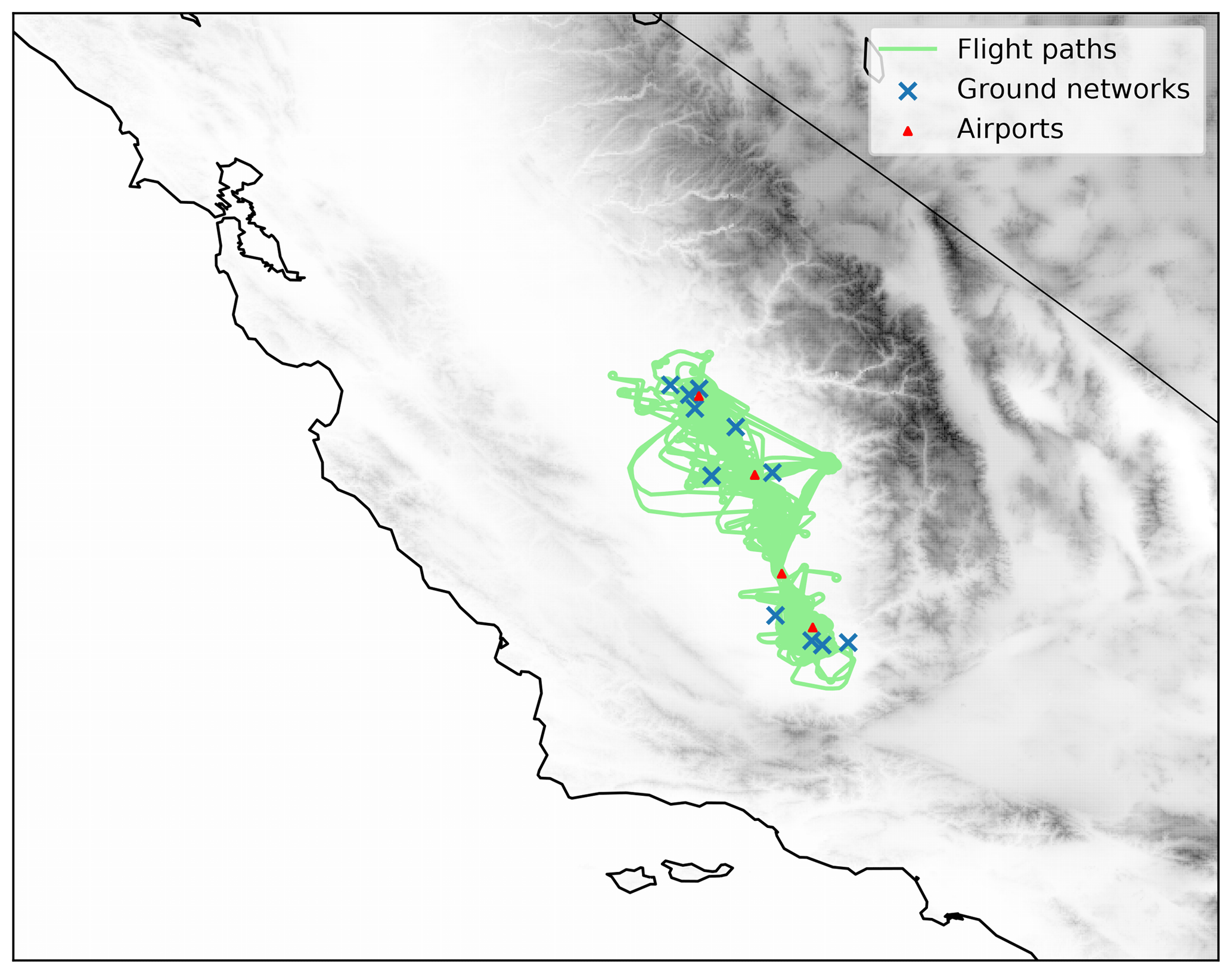
Figure 3Flight paths of all aircraft deployments in this field campaign (green). Airports where low approaches were conducted (red triangles) and with ground ozone monitors (blue crosses) are shown. From north to south, the airports are Fresno Yosemite International Airport (FAT), Visalia Municipal Airport (VIS), Delano Municipal Airport (DLO), and Bakersfield Meadows Field Airport (BFL). From north to south, the CARB ground ozone network stations are Fresno Sierra Skypark no. 2, Clovis N Villa Avenue, Fresno Garland, Fresno Drummond Street, Parlier, Visalia N Church Street, Hanford S Irwin Street, Shafter Walker Street, Bakersfield 5558 California Avenue, Edison, and Bakersfield Municipal Airport.

Download

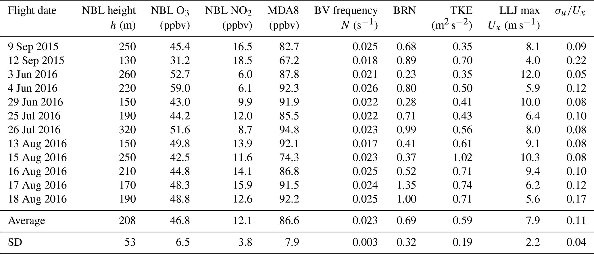
The nocturnal scalar budget analyses presented here utilize all late-night (∼21:45–00:00 PST) flights for which a subsequent flight was conducted the following morning (∼06:15–08:30 PST). The dates (before midnight PST) of the late-night flights for the 12 overnight periods are shown in Table 1. Additionally, late-night flights without a subsequent morning flight were flown on 12 September 2015 and 26 July 2016, and morning flights without a preceding late-night flight were flown on 10 September 2015, 24 July 2016, 12 August 2016, and 14 August 2016. These additional flights are included in the analyses here that refer exclusively to either the late-night or morning flights, but they were not used for the scalar budgets.

2.2 Scalar budget analysis

Here we aim to test the importance of nocturnal mixing on the ozone budget in this region by applying a scalar budgeting technique to the aircraft data in order to estimate an eddy diffusivity between the NBL and the RL. To address this objective, we use a similar method that has been presented with daytime scalar budgets (Conley et al., 2011; Faloona et al., 2009; Trousdell et al., 2016) to further demonstrate the overall practicality of this methodology.

The nocturnal budget equation is formulated by the Reynolds-averaged conservation equation for a scalar – in this case O_x – in a turbulent medium. O_x is defined here as NO₂+O₃ in order to avoid the effects of the titration of O₃ by NO. If not depleted by chemical oxidation to NO₃ and further reaction products, NO₂ will photolyze the following day to reproduce ozone in a photostationary state so it can act as an overnight reservoir of ozone. The chemical loss of O_x is then computed by the reaction between O₃ and NO₂ to form nitrate, and the ultimate fate of nitrate will affect the overall O_x loss. In the stable nighttime environment we will treat the mixing between the RL and NBL by using an eddy diffusivity. The NBL O_x budget can thus be represented as

where the term on the left represents the change in concentration with respect to time. The leftmost term on the right side of Eq. (1) represents the net loss of O_x due to chemical reaction of the resultant NO₃ and contains an unknown constant of proportionality, α, which depends on the subsequent reaction pathway of NO₃ and can range from 0 to 3. For reasons discussed later, α is assumed to be ∼1.5 for this analysis. The next two terms represent changes due to advection by the horizontal wind, followed by terms representing the dry deposition of ozone to the surface, and finally the vertical turbulent mixing term that uses the vertical gradient and the eddy diffusivity, K_z – a number that encapsulates the strength of the overnight mixing. The storage (left-hand side) term, chemical loss, advection, surface ozone, and NBL height can be calculated using the aircraft data. Combining those measurements with an estimated 0.2 cm s⁻¹ nighttime dry deposition velocity of ozone in the SSJV (an average from a study over cotton, grass, mixed deciduous forest, and vineyard field sites by Padro, 1996), we can indirectly estimate K_z. In the following sections, we detail the methods for estimating the terms in Eq. (1).

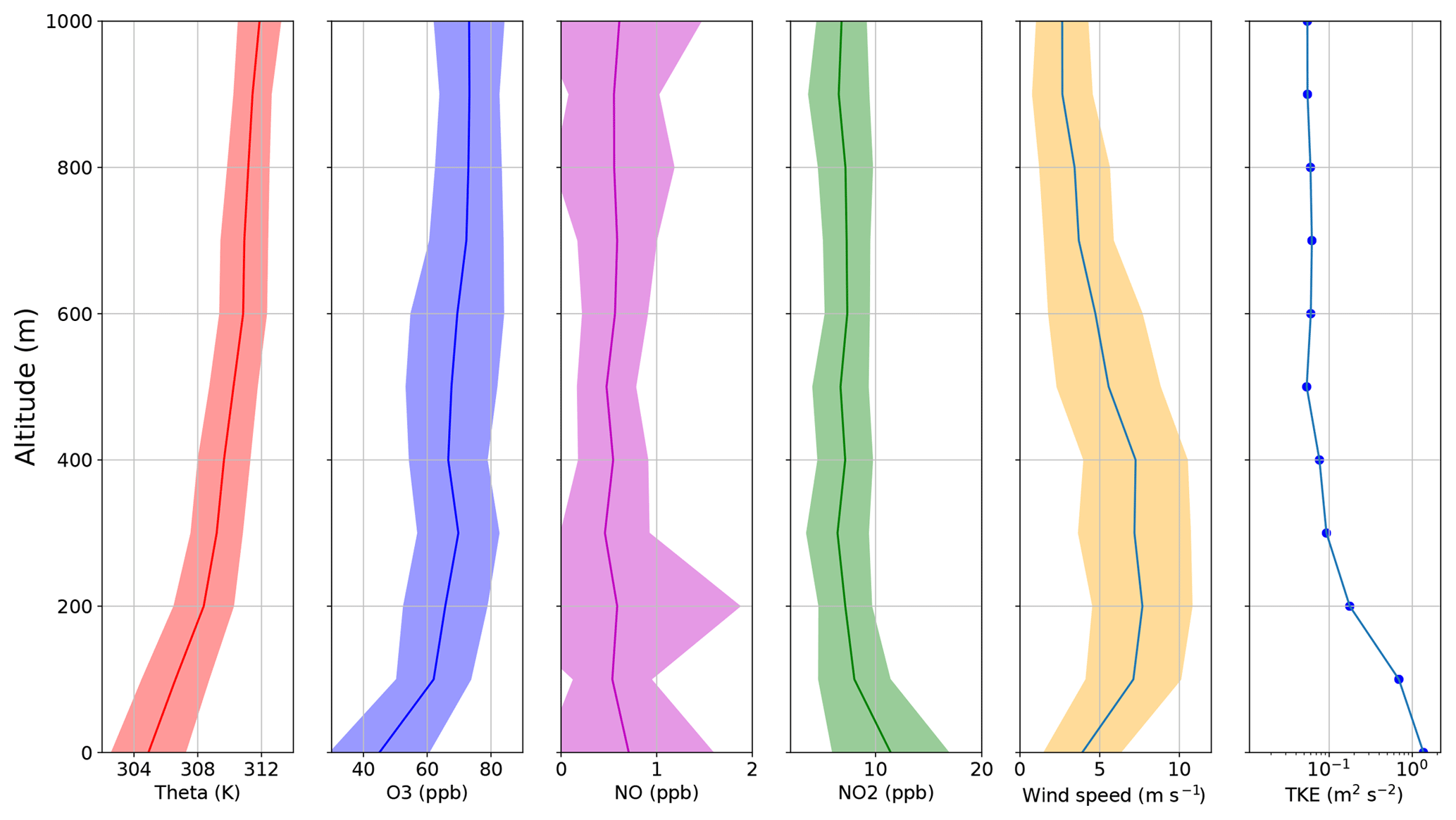
Figure 4Mean and ±1 standard deviation (swathes) of potential temperature, ozone, NO, NO₂, wind speed, and turbulent kinetic energy (mean only) from all late-night flights.

Download

2.2.1 NBL height

Profiles of wind speed, potential temperature, NO₂, and O₃ from each night and morning flight were analyzed to make a best guess of the NBL height, h. Figure 4 shows the average scalar profiles from all 15 late-night flights to illustrate the typical gradients in the lower portion of the atmosphere. One method of determining h is to observe the lowest elevation at which $\partial \mathit{\theta }/\partial z$ becomes close to adiabatic, as the layer below that physically represents air that is in thermodynamic communication with the radiatively cooled surface (Stull, 1988). Another method is to use the level of wind maximum, or LLJ height, when one is present. We found that both of these estimates typically yielded similar values of h. On nights when there was significant disagreement between the two different estimates, the vertical jump (or sharpest gradient) of O_x in the height region of the NBL–RL interface was considered, as this likely points to a region of maximum mixing. In such cases, we averaged the height at which the steepest gradient was observed with the estimates obtained from the other two methods. It should be noted that some subjectivity was involved for determining a final value of h for each night because wind maxima and thermal gradients were not always clearly defined in the profiles. All of the aforementioned factors lead to an estimated uncertainty of ±100 m for all of the NBL heights obtained. The average conditions from the late-night and morning flights are presented in Table 1.

Table 1NBL heights, ozone, NO₂, Brunt–Väisälä (BV) frequencies, bulk Richardson number (BRN), turbulent kinetic energy (TKE), and LLJ maximum wind speeds observed during the late-night and morning flight pairs. Maximum daily 8 h average ozone (MDA8) values are from the following day and are an average of the 11 ground networks in our flight region.

Download Print Version | Download XLSX

For the domain of interest, all measured NO₂ and O₃ data were averaged for each 20 m altitude bin in order to generate mean vertical profiles of O_x. Separate profiles were created for the late-night flight and the subsequent morning flight. The height of the NBL for each night (h) was used as the upper altitude limit when averaging observations to obtain advection, chemical loss, and time rate of change (storage) terms for the budget equation, since the budget equation is meant to be applied to the NBL. The overnight average O_x profile was subtracted from the sunrise profile and divided by the time difference between the midpoints of each flight to compute the storage term.

2.2.2 Nocturnal chemical loss of O_x

The chemical loss term in Eq. (1) is expected to be an important component of the NBL O_x budget. Both NO₂ and NO₃ are able to regenerate ozone in the presence of sunlight and participate in the same sequence of reactions; therefore, the species are normally grouped together into a family referred to as odd oxygen (O_x = ${\mathrm{O}}_{\mathrm{3}}+{\mathrm{NO}}_{\mathrm{2}}+\mathrm{2}{\mathrm{NO}}_{\mathrm{3}}+\mathrm{3}{\mathrm{N}}_{\mathrm{2}}{\mathrm{O}}_{\mathrm{5}}$) (Brown et al., 2006; Wood et al., 2005). However, since we did not measure NO₃ and N₂O₅, in this study we estimate O_x as merely the sum of O₃+NO₂ because these are expected to exceed to concentrations of the other O_x species by 1–2 orders of magnitude (Brown et al., 2003; Smith et al., 1995). Considering O_x is useful for our study because the family is conserved in the rapid oxidation of NO by O₃ (Reaction R1 below) yielding NO₂, which may be quickly photolyzed to regenerate O₃ once the sun rises as part of the standard daytime photostationary state.

Aside from dry deposition to the Earth's surface, NO_x chemistry is the main loss of ozone at night, counteracting its role in production during the daytime (Brown et al., 2006, 2007). The chemical loss of ozone at night begins with the production of the nitrate radical (Reaction R2).

$$\begin{array}{}\text{(R1)}& {\displaystyle }& {\displaystyle }\mathrm{NO}+{\mathrm{O}}_{\mathrm{3}}\to {\mathrm{NO}}_{\mathrm{2}}+{\mathrm{O}}_{\mathrm{2}}\text{(R2)}& {\displaystyle }& {\displaystyle }{\mathrm{NO}}_{\mathrm{2}}+{\mathrm{O}}_{\mathrm{3}}\to {\mathrm{NO}}_{\mathrm{3}}+{\mathrm{O}}_{\mathrm{2}}\end{array}$$

NO₃ photolyzes rapidly once the sun rises, so the ultimate net loss of ozone depends on the loss of nitrate in the dark. The loss occurs mainly via three general channels. In one channel, dinitrogen pentoxide is formed (Reaction R3), which has a backwards reaction and can be a source of NO₂ if not deposited onto moist surfaces or aerosols to form nitric acid via hydrolysis (Reaction R4).

$$\begin{array}{}\text{(R3)}& {\displaystyle }& {\displaystyle }{\mathrm{NO}}_{\mathrm{3}}+{\mathrm{NO}}_{\mathrm{2}}+\mathrm{M}\leftrightarrow {\mathrm{N}}_{\mathrm{2}}{\mathrm{O}}_{\mathrm{5}}+\mathrm{M}\text{(R4)}& {\displaystyle }& {\displaystyle }{\mathrm{N}}_{\mathrm{2}}{\mathrm{O}}_{\mathrm{5}}+{\mathrm{H}}_{\mathrm{2}}\mathrm{O}\to \mathrm{2}{\mathrm{HNO}}_{\mathrm{3}}\text{(Net (R1-R4))}& {\displaystyle }& {\displaystyle }\mathrm{NO}+\mathrm{2}{\mathrm{O}}_{\mathrm{3}}+{\mathrm{NO}}_{\mathrm{2}}\to \mathrm{2}{\mathrm{NO}}_z\end{array}$$

${\mathrm{NO}}_z={\mathrm{NO}}_y-{\mathrm{NO}}_x$ represents the family of products of NO_x oxidation. In another channel, nitrate is lost by reaction with a wide array of organic compounds. This process can typically be represented by Reaction (R5), but in some cases, organic compounds can become rearranged to produce an NO₂ molecule (Reactoin R5a) (Brown et al., 2006).

$$\begin{array}{}\text{(R5)}& {\displaystyle }& {\displaystyle }{\mathrm{NO}}_{\mathrm{3}}+(\mathrm{VOC},\mathrm{etc}.)\to \mathrm{organic}\mathrm{nitrates}\text{(R5a)}& {\displaystyle }& {\displaystyle }{\mathrm{NO}}_{\mathrm{3}}+(\mathrm{VOC},\mathrm{etc}.)\to \mathrm{organic}\mathrm{nitrates}+{\mathrm{NO}}_{\mathrm{2}}\text{(Net (R1, R2, R5))}& {\displaystyle }& {\displaystyle }\mathrm{NO}+\mathrm{2}{\mathrm{O}}_{\mathrm{3}}\to {\mathrm{NO}}_z\text{(Net (R1, R2, R5a))}& {\displaystyle }& {\displaystyle }\mathrm{NO}+\mathrm{2}{\mathrm{O}}_{\mathrm{3}}\to {\mathrm{NO}}_z+{\mathrm{NO}}_{\mathrm{2}}\end{array}$$

However, in urban environments with nocturnal sources of NO, nitrate is reduced back to NO₂ by very rapid reaction.

$$\begin{array}{}\text{(R6)}& {\displaystyle }& {\displaystyle }\mathrm{NO}+{\mathrm{NO}}_{\mathrm{3}}\to \mathrm{2}{\mathrm{NO}}_{\mathrm{2}}\text{(Net (R1, R2, R6))}& {\displaystyle }& {\displaystyle }\mathrm{2}\mathrm{NO}+\mathrm{2}{\mathrm{O}}_{\mathrm{3}}\to \mathrm{2}{\mathrm{NO}}_{\mathrm{2}}\end{array}$$

If the hydrolysis of N₂O₅ (Reaction R4) is the dominant NO₃ sink, then the net reaction leads to a loss of three O_x molecules per nitrate produced (Reaction R2). However, if the dominant loss is reaction with VOCs then the net reaction leads to between one (Reaction R5a) and two (Reaction R5) O_x molecules lost per R2. And if there is sufficient NO, Reaction (R6) will dominate the nitrate loss, leading to no net O_x loss per Reaction (R2). Thus, determining the dominant loss of nitrate is crucial for any analysis of the diurnal budget of ozone.

Reaction (R6) has often been ignored at night under the presumption that local sources of NO are sparse and Reaction (R1) will outcompete Reaction (R6) (Brown et al., 2007; Stutz et al., 2010). However, at observed values of 30 ppb of O₃ and an estimated 20 ppt of NO₃ (Smith et al., 1995), the lifetime of NO (∼80s) with respect to Reaction (R1) would be nearly equivalent to that of Reaction (R6). Our measurements indicate ground-level NO of about 0.6 ppb at midnight (σ=1 ppb), corroborated by the CARB surface air quality network, increasing in the early morning hours to 2–4 ppb. However, both the ground network and aircraft observations may be biased high to the regional average because of their proximity to California Highway 99 and other urban centers (Fig. 3). Nevertheless, the rate of Reaction (R6) is $\mathrm{2.6}\times {\mathrm{10}}^{-\mathrm{11}}$ cm³ s⁻¹ molec⁻¹ (Sander et al., 2006), extremely rapid relative to the others, such that even 60 ppt of NO (an order of magnitude lower than what our measurements indicate) would result in an NO₃ lifetime of only 25 s. Hence, we conclude that Reaction (R6) should not be ignored in general as it may ultimately reduce the chemical loss rate of O_x overnight.

There is then a further question as to whether any VOCs would be able to compete with this channel of NO₃ consumption. An investigation into the most rapid VOC reactions with NO₃ per Atkinson et al. (2006) and Gentner et al. (2014a) is presented in Table 2. In this analysis, concentrations of VOCs are estimated from available reports in the SJV, which given its roughly 5 million acres of irrigated land (Li et al., 2016) may vary widely from one location to another due to the presence of diverse crop canopies. The estimated lifetime of NO₃ due to the VOC reactions in Table 2 is 12.2 s, about 5 times the lifetime of NO₃ with respect to the presence of 0.6 ppb of NO (2.5 s). We note that although there are few direct observations of NO₃ in the SSJV, the CalNex campaign conducted one flight that measured concentrations of about 10–40 ppt shortly after sunset on 24 May 2010 (https://esrl.noaa.gov/csd/groups/csd7/measurements/2010calnex/P3/DataDownload/index.php, last access: 30 April 2018). Smith et al. (1995) present DOAS measurements from 15 nights in July and August 1990 (their Fig. 6a) from a site 32 km southeast of Bakersfield suggesting that NO₃ concentrations in the SSJV peak around 30 pptv within an hour or two after sunset and plateau in the middle of the night around 10 ppt, then decline to zero by sunrise. The variability of NO₃ reported in that study is high, with nocturnal values ranging from near zero to over 50 ppt. Under a simplified, steady-state model, the expected lifetime of NO₃ can be estimated using the second-order reaction rate for Reaction (R2) for the formation of the nitrate radical and combining all of the loss channels into a single lifetime (${\mathit{\tau }}_{{\mathrm{NO}}_{\mathrm{3}}})$:

$$\begin{array}{}\text{(2)}& {\mathit{\tau }}_{{\mathrm{NO}}_{\mathrm{3}}}={\displaystyle \frac{\left[{\mathrm{NO}}_{\mathrm{3}}\right]}{k_{\mathrm{2}}\left[{\mathrm{NO}}_{\mathrm{2}}\right]\left[{\mathrm{O}}_{\mathrm{3}}\right]}}.\end{array}$$

Using the average NBL ozone and NO₂ from Table 1, an NO₃ concentration of 10 ppt would imply its lifetime to be about 25 s, which is about twice as large as our estimate from Table 2. Based on these direct measurements of NO₃, our lifetime calculations likely represent a lower bound and further illustrate the uncertainty given the sensitivity to the unconstrained VOCs and our NO measurements, which have an envelope of error that spans a large range of possible nitrate loss lifetimes.

Table 2Estimations of VOC reactions with nitrate in the summertime nocturnal boundary layer for the SSJV. Reaction rates from Atkinson and Arey (1998), Table 2, and Atkinson et al. (2006).

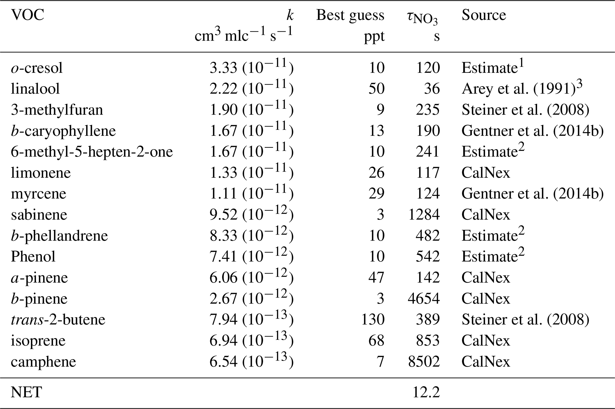
¹ Drew Gentner of Yale University, personal communication. ² No measurements reported in the SSJV; an order of magnitude estimate is made based on typical aerosol concentrations. ³ Arey et al. (1991) reported 70 ppt in an orange grove. We estimate 50 ppt as an SJV average.

Download Print Version | Download XLSX

With longer lifetimes of nitrate loss with respect to the VOC and NO reactions, we are faced with the possibility that the hydrolysis of N₂O₅ is also an important loss channel, increasing the amount of O_x molecules lost per nitrate molecule formation in Reaction (R2). Smith et al. (1995) report that the lifetime of NO₃ was found to be highly dependent on relative humidity, with lifetimes ranging from seconds to 10 min when the relative humidity is above 45 % (presumably due to N₂O₅ hydrolysis) but between 10 and 60 min when below the 45 % threshold. Figure 5 shows the diurnal cycle of temperature and relative humidity observed at the airports in our flight region during the days of our campaign compared with the 2015–2016 1 June–30 September averages. The >45 % relative humilities observed at FAT and VIS imply that the hydrolysis of N₂O₅ is an important sink for NO₃.

Given the importance of nitrate loss to VOCs and NO, but some importance of the N₂O₅ hydrolysis, we use a best estimate that each effective collision of NO₂ and O₃ will lead to the net loss of approximately 1.5(±0.5) molecules of O_x from the net effects of the entire series of reactions outlined above. This is a “center of the envelope” estimate for the possible range of 0–3. Although our measurements are unable to constrain this coefficient, the ultimate fate of the nitrate radical can be seen to have a critical role in quantifying the net loss of O_x overnight, and without a greater understanding of the nitrate budget, predicting this loss rate is uncertain.

Consequently, we calculate the net Reaction (R1–R6) for the nocturnal chemical loss rate of O_x as a constant multiple of Reaction (R2). The second-order rate equation for the net chemical loss of O_x is calculated by

$$\begin{array}{}\text{(3)}& {\left.{\displaystyle \frac{\mathrm{d}{\mathrm{O}}_x}{\mathrm{d}t}}\right|}_{\mathrm{chemical}\mathrm{loss}}=-\mathit{\alpha }{k}_{{\mathrm{O}}_{\mathrm{3}}+{\mathrm{NO}}_{\mathrm{2}}}\left[{\mathrm{O}}_{\mathrm{3}}\right]\left[{\mathrm{NO}}_{\mathrm{2}}\right],\end{array}$$

where α can range from 0 to 3 and, per the discussion above, is estimated to be 1.5±0.5 (uncertainty discussed in Sect. 3.2). To estimate a value for the second-order rate constant ($k_{{\mathrm{O}}_{\mathrm{3}}+{\mathrm{NO}}_{\mathrm{2}}})$, we start with the temperature-dependent function for this reaction (Sander et al., 2006):

$$\begin{array}{}\text{(4)}& k_{{\mathrm{O}}_{\mathrm{3}}+{\mathrm{NO}}_{\mathrm{2}}}=\mathrm{1.2}\left({\mathrm{10}}^{-\mathrm{13}}\right)\cdot e^{\frac{-\mathrm{2450}}{T}},\end{array}$$

where T is the temperature in Kelvin. For the domain being analyzed, an instantaneous value of $k_{{\mathrm{O}}_{\mathrm{3}}+{\mathrm{NO}}_{\mathrm{2}}}$ is determined at each data point. These values of $k_{{\mathrm{O}}_{\mathrm{3}}+{\mathrm{NO}}_{\mathrm{2}}}$ are then averaged to obtain a constant value for the given night. It should be noted that small errors in the value of k that are within the order of our temperature fluctuations were found not to have a measurable impact on the chemical loss term. To estimate the chemical loss of O_x, the initial 20 m altitude bins for NO₂ and O₃ are taken from the late-night and morning profiles. In each bin, the concentrations are linearly interpolated between the late-night and morning values so that there is an estimation of the current average concentration within that bin at every time during the night.

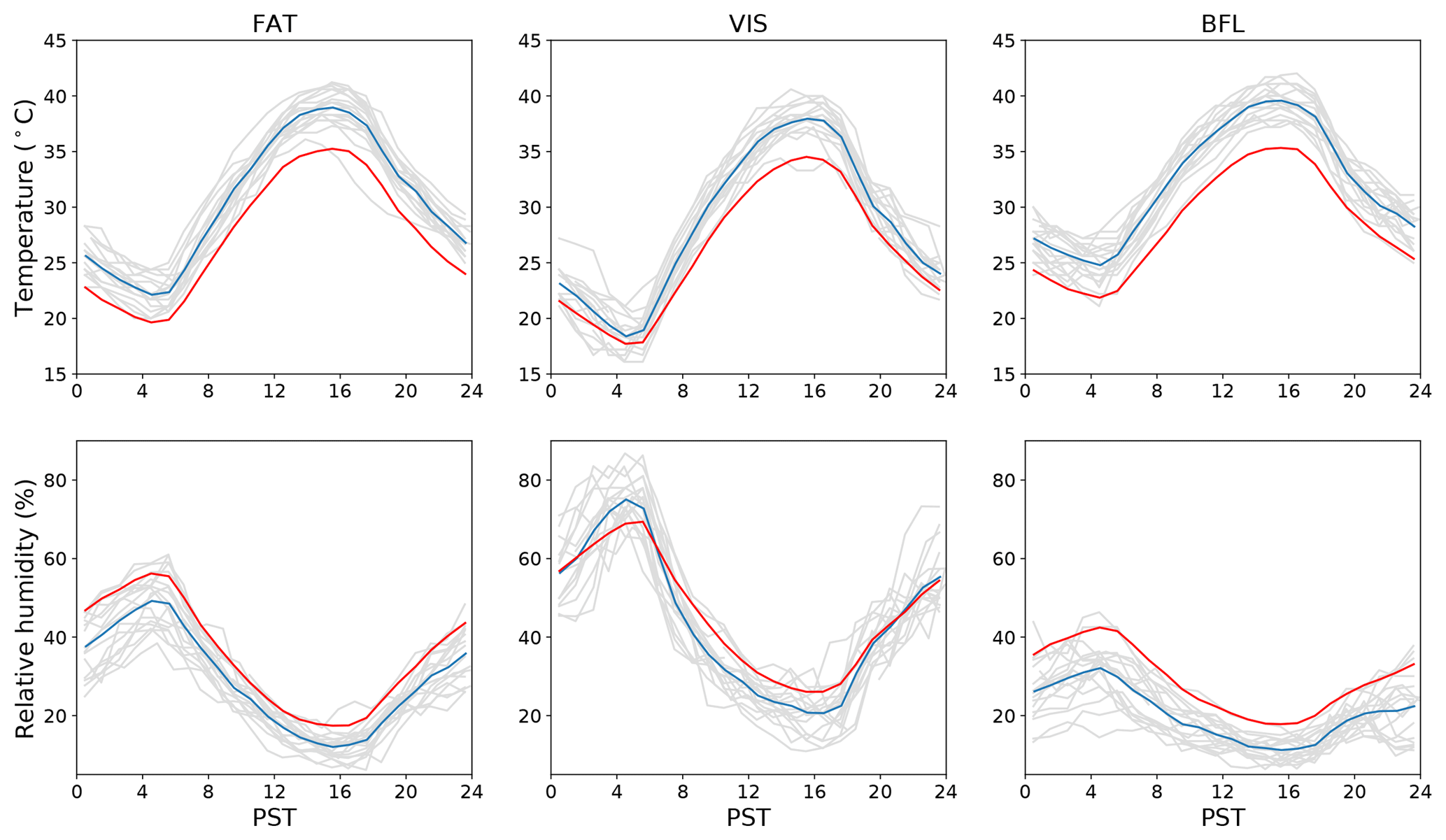
Figure 5Diurnal plots of temperature and relative humidity during flight days of the Residual Layer Ozone campaign (individual days: grey lines, campaign average: blue lines) compared to 1 June–30 September 2015 and 2016 averages (red lines) at the Fresno (FAT), Visalia (VIS), and Bakersfield (BFL) airports as part of the Automated Weather Observing System (AWOS) network. Hours are in Pacific Standard Time (PST).

Download

2.2.5 Vertical turbulent mixing between the NBL and the RL

Finally, a vertical flux divergence for O_x must be estimated for Eq. (1), which is represented by the last two terms. For the top part of the NBL, the flux of O_x can be interpreted as an eddy diffusivity (K_z) multiplied by the vertical gradient of O_x between the NBL and RL. For each flight, a linear regression through the 1 s O_x data within the NBL–RL interface is used to determine ∂$\left[{\mathrm{O}}_x\right]/\partial$z (for the last term in Eq. 1) in the upper portion of the NBL that appeared to contain the strongest O_x gradient. The average r² value of the 24 regressions was 0.11, and the number of data points that they contained ranged from 116 to 2166. Typical values of the vertical O_x gradients were $\sim \mathrm{0.07}\pm \mathrm{0.04}$ ppb m⁻¹. The layers used for the regression fit were 100–200 m thick and did not extend below 70 m a.g.l. to avoid capturing the region where the O_x sink due to surface deposition and/or reaction with freshly emitted NO likely accounts for the vertical gradient in O_x (Fig. 6). The eddy diffusivity can now be solved for with all of the other terms estimated.

The contribution of vertical mixing to the budget can be visualized as an inferred difference between O_x profiles that are observed and O_x profiles that are predicted from other terms in Eq. (1). Figure 6 shows an example of the observed profiles of O_x on the late-night and morning flights for the series performed on 4 June 2016. The height of the NBL is shown (green), and the lower bound of the layer used in the vertical gradient fit is shown (yellow). The dashed profiles show the expected profile that would have been observed on the morning flight if only advection (blue), chemical loss (green), or both advection and chemical loss (red) processes were occurring. The observed morning O_x (magenta) is inferred to exceed the predicted morning O_x (red) due to the vertical mixing term in the scalar budget equation.

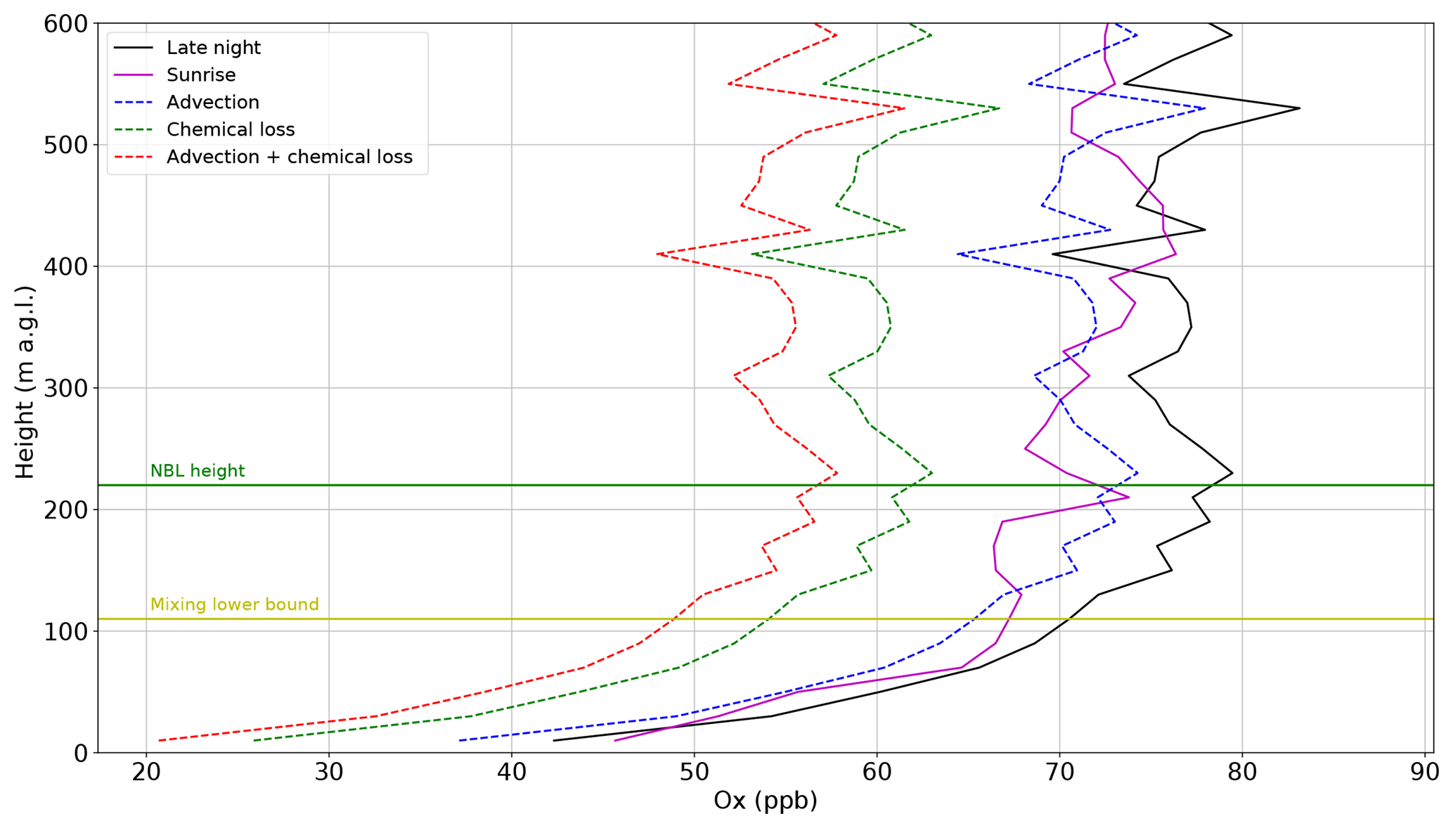
Figure 6O_x profiles from 4 June 2016 overnight analysis, NBL height (green line), and lower bound to vertical mixing gradient (yellow line). The solid lines are observations and the dashed lines are calculated based on expected changes due to horizontal advection (blue), chemical loss (green), and the sum of the two (red).

Download

3.1 O_x scalar budget results

Results of the scalar budget analysis for all 12 paired late-night and morning flights are presented in Table 3. An error propagation analysis (discussed in Sect. 3.2) is presented for each term in the budget, and for the K_z values.

Table 3Results from the nocturnal scalar budget for all terms. Estimated error (see Sect. 3.2) in parenthesis.

Download Print Version | Download XLSX

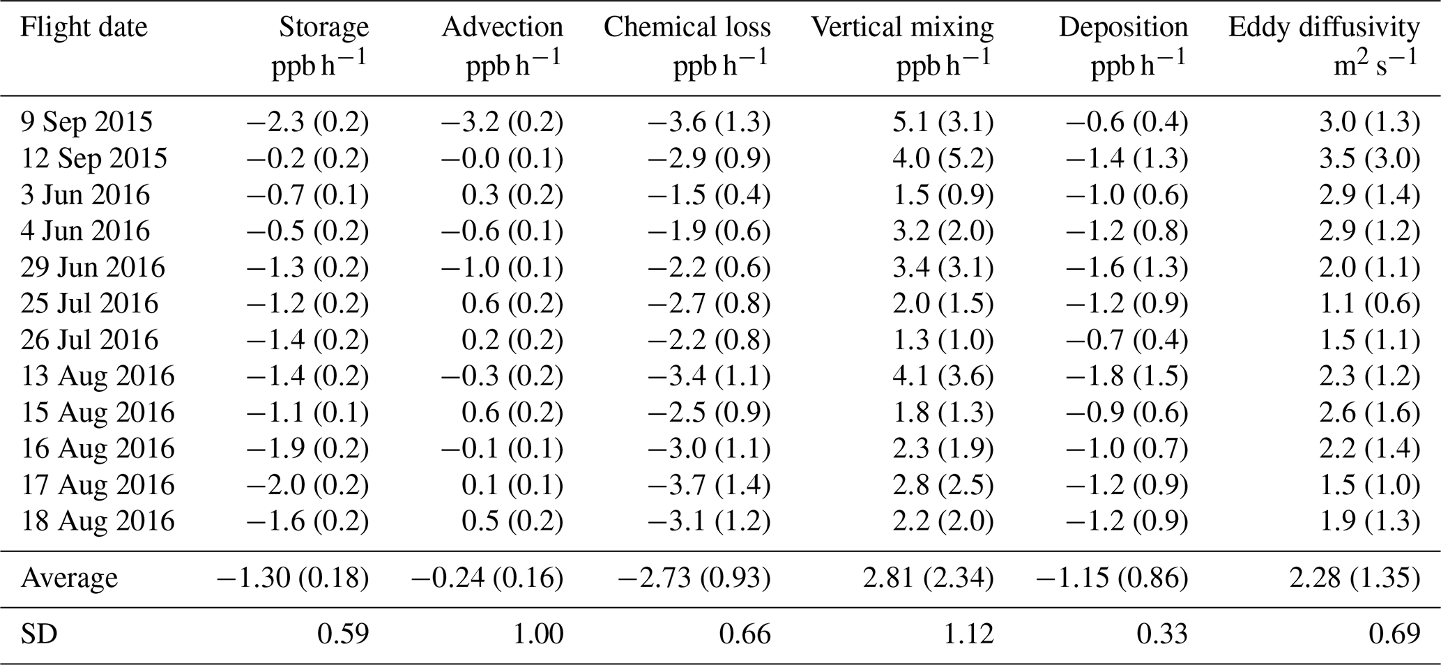
Of note is the fact that, on average, the chemical loss is expected to be a little more than twice as large as the physical loss from dry deposition. For dry deposition, the average lifetime of ozone is 28 h (200 m ∕ 0.002 m s⁻¹), and for chemical loss it is 12 h. Both losses of O_x added together are about triple the observed time rate of change, and thus the physical and chemical losses are largely ($\sim \mathrm{2}/\mathrm{3}$) compensated for by vertical mixing. Because the RL consistently contains more ozone than the stable NBL, turbulent mixing will result in a transfer of ozone into the NBL. While NO₂ is observed to be higher in the NBL than in the RL (by about 3–5 ppbv), it is a much smaller contribution to O_x (O₃ is less than NO₂ by anywhere from 10 to 20 ppbv.) Thus, vertical mixing at the top of the NBL, influenced by the strength of the LLJ, is inherently a source term of O_x to the lower NBL.

3.2 Error analysis

Here we estimate the uncertainties for each term in the budget equation and those for the resultant eddy diffusivities. The storage term error is computed by first taking the standard deviation of 1 s ozone measurements divided by the square root of the number of samples, then the standard error of the means for both the late-night and morning profiles are combined. This analysis is carried out in 20 m altitude bins separately and then averaged together because there is more uncertainty at lower altitudes due to fewer measurements. The advection term error is computed from the standard error of the slopes of the regression fit, with errors propagating for each of the four advection components for both the u and v components of wind. To compute the chemical loss error, the large uncertainty of the α coefficient must be taken into consideration. Based on our analysis concluding that all channels of nitrate loss are probably non-negligible, we infer that α is between 0.5 and 2.5 with a 95 % confidence interval. Thus, 1 standard error for the α coefficient is about 0.5. An error propagation is then carried out for each 20 m altitude bin using the standard deviations of the O₃ and NO₂ measurements divided by the square root of the sample size. As previously stated, the estimated standard errors of the NBL height and surface deposition of ozone are taken to be 100 m and 0.1 cm s⁻¹, respectively. The surface ozone standard error is computed as the standard deviation of the aircraft measurements divided by the square root of the sample size, and the vertical O_x gradient uncertainty is computed by the standard error of the regression slope. The uncertainties in the vertical mixing, deposition flux, and diffusivity values can then be computed by standard error propagation. The resultant relative error estimates of the nighttime diffusivities are about 50 %, and errors of this order seem reasonable based on a technique that assumes the closure of four independently measured terms. Past studies using similar airborne budgeting methods have estimated relative uncertainties ranging from 15 % to 75 % (Conley et al., 2011; Faloona et al., 2009; Kawa and Pearson, 1989; Trousdell et al., 2016).

3.3 The Fresno eddy and LLJ

The formation of the Fresno eddy begins when the daytime northwesterly valley wind continues into the late evening, decoupling from the surface and forming an LLJ (Davis, 2000). The Tehachapi Mountains will typically topographically block the flow of the LLJ (Lin and Jao, 1995). The eddy is formed during the hours before dawn when this northwesterly flow interacts with southeasterly nocturnal downslope flow coming from the high southern Sierra Nevada Mountains, although there is some question as to the extent to which the southeasterly flow observed in the morning hours is merely the result of a topographic deflection and recirculation of the nocturnal jet. The Coriolis force helps to circulate this flow; however, a mesoscale low is not thought to develop (Bao et al., 2008; Lin and Jao, 1995). We note that the valley flow peaks around midnight, while the katabatic drainage flow peaks near dawn, so these two components of the Fresno eddy are not time coherent. The initial northwesterly wind and a topographic blockage are both critical for determining whether or not the eddy will form on a given night (Lin and Jao, 1995).

One complicating factor for our scalar budget analysis is the influence that this eddy will have on our measurements of advection. If an eddy is recirculating a scalar quantity, using a simple linear fit model as we did in Sect. 2.2.3 to estimate advection would be questionable, especially if the flight area only covered a small portion of the larger mesoscale circulation. Zhong et al. (2004) use a series of 915 MHz RASSs to analyze low-level winds in the SSJV. Their Fig. 4 shows that at night, the northwesterly LLJ is formed in the SJV, and a weak katabatic southerly flow is observed in the foothills to the east at the Trimmer site. As the night progresses, the eddy becomes more coherent as the northwesterly jet relaxes, while the southerly flow strengthens and expands westward. After daybreak, the eddy appears to deform and disintegrate, with much of the SSJV experiencing a strong southerly wind.

This pattern is roughly consistent with our aircraft observations, suggesting the presence of a Fresno eddy during our flights. An analysis of the average wind vectors and their consistency for all nocturnal and morning flights in the approximate NBL (0–300 m a.g.l.) and RL (300–700 m a.g.l.) is shown in Fig. 7. The wind consistency is defined as the ratio of the vector-averaged wind speed to the magnitude-averaged wind speed, with values close to 1 indicating a consistent wind direction (Stewart et al., 2002; Zhong et al., 2004). The nocturnal LLJ can clearly be seen to fill most of the SSJV in both the NBL and RL. In the morning RL, there is localized consistent southerly flow closest to the foothills, some of which may be regarded as surprisingly strong. The lower-level winds in the morning are consistent with the deformed eddy. We note that caution should be exercised in directly comparing our flight data to the analysis from Zhong et al. (2004) as our flights specifically targeted high-ozone events, which we based primarily on high temperature stagnation conditions (see Fig. 5). Thus, the synoptic and mesoscale conditions during our flights may be systematically different from the climatological norms presented in Zhong et al. (2004).

From this analysis, we conclude that it is likely that our dataset captures the bulk of the dominant flow (and thus advection) on both the late-night and morning flights, which are averaged and interpolated. The average advection term for the 12 nights presented is −0.24 ppb h⁻¹, which is nearly an order of magnitude smaller than the chemical loss and storage terms. The small average contribution from advection is consistent with previous findings from daytime scalar budgets performed over the oceans (Conley et al., 2011; Faloona et al., 2009) and in the SJV (Trousdell et al., 2016) and what might be expected in the presence of a recirculating eddy. Lastly, it is noted that individually adjusting each flight to have an advection term of zero (to assume full eddy recirculation) results in only a 3 % change to the average of the diffusivity values, which further supports the idea that the influence of advection on our scalar budget analysis is minimal.

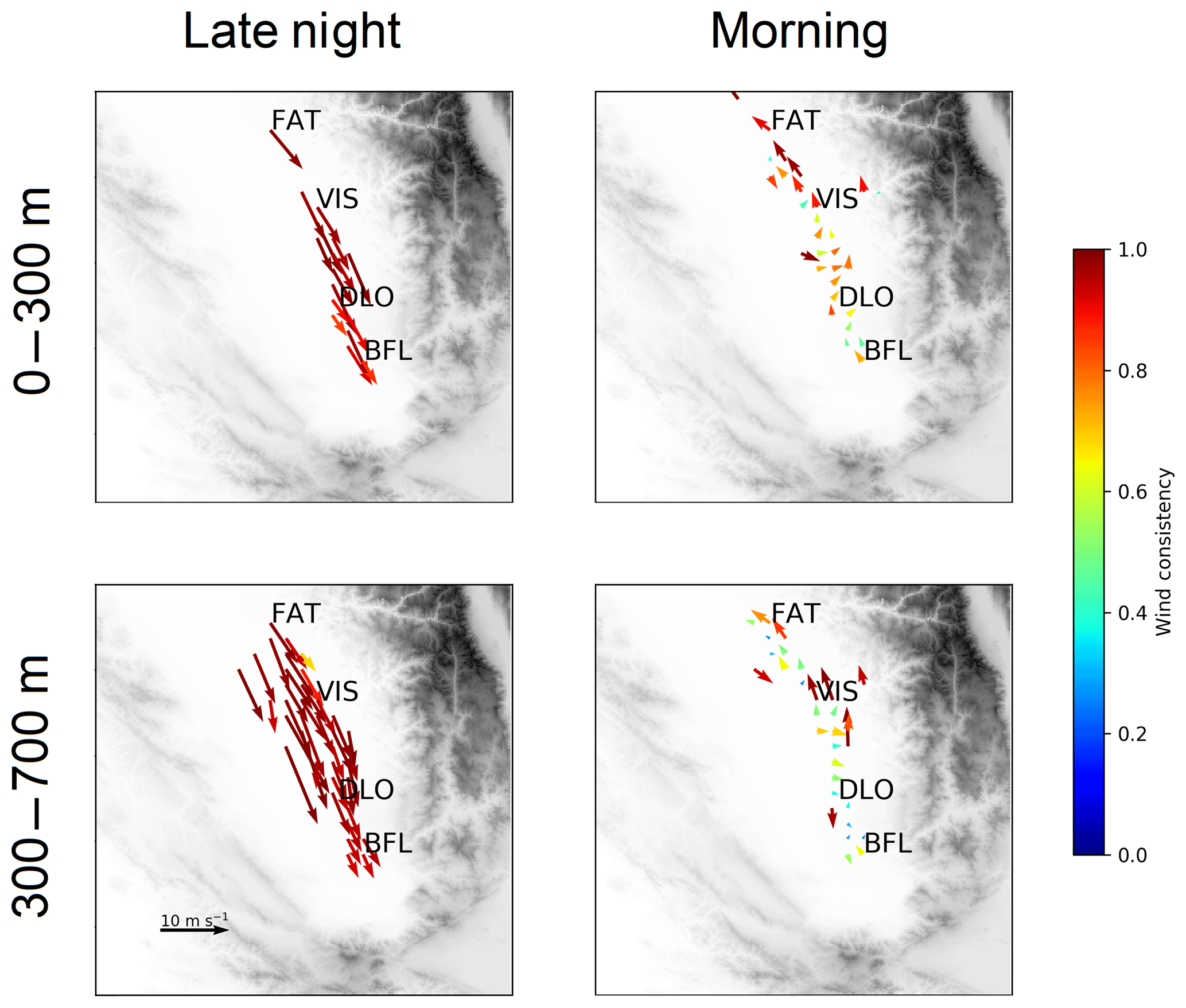
Figure 7Wind consistency for late-night flights and morning flights in the NBL (0–300 m) and the RL (300–700 m).

Download

Since the LLJ is hypothesized to contribute to the variability of maximum daytime ozone concentration, we explored the synoptic patterns that are associated with differing strengths of the LLJ. A total of 7 years of data (2010–2016) from the 915 MHz sounder located in Visalia, CA, are compiled to obtain the LLJ speed and the height at which it was observed. For this analysis, we define the nocturnal LLJ speed as the maximum hourly averaged wind speed observed below 1000 m averaged in 100 m vertical bins from 23:00 to 07:00 PST, specifically during the summer months (defined here as 1 June–30 September). The 1000 m cutoff is used to ensure that the wind maximum captured is related to the LLJ at the top of the NBL rather than free-tropospheric wind. Using this definition, the LLJ had an average height of 340 m, an average speed of 9.9 m s⁻¹ (σ=3.1 m s⁻¹), and a typical peak timing around 23:00 PST. The 700 mb level corresponds to approximately 3000 m, well above the Pacific Coast Range but approximately in line with the top of the southern Sierras.

To analyze possible synoptic influences on the jet strength, daily average synoptic charts from the North American Regional Reanalysis (NARR) are created in Figs. 8 and 9 for days when the LLJ strength was less than 7 m s⁻¹ (N=147 nights) and greater than 12 m s⁻¹ (N=165 nights). Both the strong and weak low-level jets show a climatological trough pattern, but the mean trough axis is situated about 100 km to the east for the strong cases (Fig. 8b). We also note that the pressure gradient is at least twice as strong for the stronger low-level jets and that the synoptic pattern of the weak jets favors a southerly geostrophic wind aloft, which directly opposes the up-valley northwesterly thermally driven flow. We also find a positive correlation between the LLJ strength and the upwelling index (r²=0.3018, $p<{\mathrm{10}}^{-\mathrm{5}})$, calculated by NOAA's Pacific Fisheries Environmental Lab at 33^∘ N, 119^∘ W (https://www.pfeg.noaa.gov/products/PFEL/modeled/indices/upwelling/NA/upwell_menu_NA.html, last access: 8 August 2018). The indices are primarily driven by the strength and position of the North Pacific High, which, when strong, acts to push the 700 mb trough farther eastward, as seen in Fig. 8b, and is associated with lower sea surface temperatures and thus enhanced thermal forcing of the coupled sea breeze and valley wind. These findings are consistent with the Lin and Jao (1995) modeling study that showed that the Fresno eddy (and associated LLJ) did not form when the synoptic flow over the coastal range was westerly. Beaver and Palazoglu (2009) found that maximum daily 8 h average ozone (MDA8) exceedances were more frequent in the central and southern San Joaquin Valley when an offshore ridge or onshore high was present, consistent with Fig. 8a. The results of our study suggest that this may be at least partially explained by the presence of a weaker LLJ under those synoptic conditions.

Although the LLJ and Fresno eddy are not synonymous, we propose that the northwesterly LLJ could be the dominant feature of the eddy's northerly flow component. This leads to an important question about the role of the Fresno eddy in modulating the daily ozone peak. Beaver and Palazoglu (2009) purport that ozone levels in the central SJV are particularly high on days when the morning southerly wind at Parlier, a site about midway between Fresno and Visalia, is strong, concluding that recirculation from the downslope branch of the Fresno eddy significantly controls the day's buildup of ozone. However, mixing induced by LLJs in other parts of the world has been shown to decrease ozone levels the following day (Hu et al., 2013; Neu, 1995). Thus, it may be the case that a Fresno eddy associated with a particularly strong LLJ may decrease ozone the following day if the recirculation of ozone and its precursors does not overcompensate for overnight losses due to vertical mixing down to the surface. We suggest that the Fresno eddy, when present, will act to recirculate pollutants regardless of the strength of the LLJ. That is, a stronger eddy will not recirculate pollutants any more than a weaker one will. Thus, the nighttime dynamical conditions that will lead to the greatest ozone levels the following day may consist of a Fresno eddy just coherent enough to effectively recirculate pollutants, but without an associated LLJ so strong as to deplete the RL ozone by vertical mixing. There is currently no established link in the literature between the Fresno eddy and LLJ strength. Thus, future research should investigate which of these two nocturnal mechanisms (recirculation from the eddy or RL depletion by vertical mixing) will dominate the ozone budget on any given night, taking into consideration the different possible structures and timing of the Fresno eddy as well as the synoptic conditions that engender them.

In addition to the synoptic patterns discussed above, slightly lower surface temperatures across the entire region are observed during stronger LLJs (Fig. 9). This could either be a consequence of the synoptic flow (southerly geostrophic flow will generally bring warm air advection) or itself be an underlying precursor to the LLJ. In the latter case, a ∼2 K greater temperature difference between the delta region and the SSJV for strong LLJs (seen in Fig. 9) will lead to more up-valley thermal forcing, resulting in stronger winds that decouple from the surface at night. The higher temperatures associated with the weak nocturnal jets may make for a twofold mechanism for high ozone: the high temperatures either cause increased photochemical production or result from increased meteorological stagnation, and a lack of mixing overnight induced by the LLJ causes less depletion of the RL ozone. Warmer nights may also result in less dry deposition of O_x through stomatal pores.

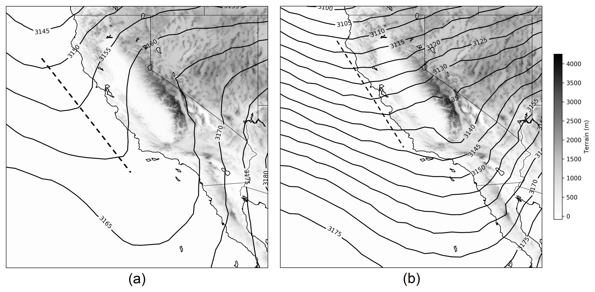
Figure 8North American Regional Reanalysis 700 mb geopotential height (m) for low-level jet speeds less than 7 m s⁻¹ (a) and greater than 12 m s⁻¹ (b).

Download

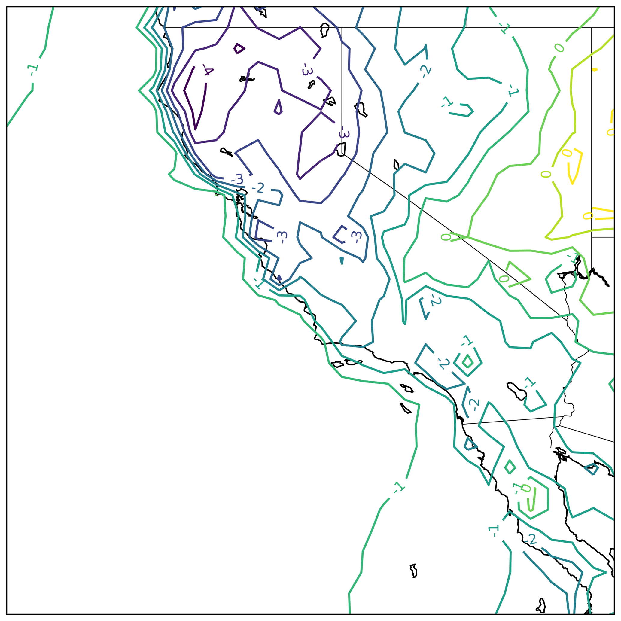
Figure 9North American Regional Reanalysis 2 m air temperature (^∘C) difference between cases in which the low-level jet speed exceeds 12 m s⁻¹ and cases in which it is below 7 m s⁻¹ at 01:00 PST. Positive values indicate warmer surface temperatures for strong jets.

Download

3.4 Vertical mixing and next-day ozone

As seen in Fig. 4, the average LLJ height is 200–400 m, which approximately corresponds to the average NBL depth. Likely due to the shear induced by the LLJ, turbulence is seen to be vigorous at night with TKE values about 50 % of daytime values during convective conditions. Further, TKE increases toward the surface, a condition that Banta et al. (2006) refer to as a “traditional” stable boundary layer. As previously mentioned, the physical significance of turbulent mixing overnight in relation to SJV air pollution remains somewhat of an open question. On the one hand, Beaver and Palazoglu (2009) suggest that a stronger Fresno eddy circulation is associated with higher ozone pollution. On the other hand, greater coupling between the NBL and RL, induced by turbulence generated from the LLJ, could reduce the amount of ozone stored in the RL reservoir, rendering cleaner air the following day. To test this hypothesis, the relationship between the eddy diffusivity values found in our study and regional mean surface ozone from the CARB network is analyzed.

The thermals generated by solar heating after sunrise initiate a fumigation process whereby as the daytime boundary layer develops, the ozone that was in the RL is mixed downward. The change in surface ozone concentration (d[O₃]∕dt) due to fumigation peaks at around 08:00 PST and continues until about 10:00. The relationship between our estimated eddy diffusivities and ozone during the fumigation period is strongest at 10:00 PST, after the bulk of the fumigation has occurred (r²=0.29, p=0.07). A negative correlation between eddy diffusivities and the maximum 1 h ozone, 24 h average ozone, and MDA8 was also found, with the strongest relationship for the MDA8 (r²=0.46, p=0.015), as shown in Fig. 10. This supports our hypothesis that stronger NBL turbulence is associated with lower ozone the following day.

Figure 10Correlation between overnight eddy diffusivity and maximum daily 8 h average ozone (MDA8) the following day. All values are averages of 11 CARB surface network stations that are within the flight region.

Download

Because this analysis consisted of only 12 flights, we explored a larger dataset that might support the hypothesis that a stronger LLJ reduces ozone the following day. A total of 7 years of LLJ speeds obtained from the Visalia sounder from 2010–2016 are combined with the CARB surface network ozone monitoring site at Visalia N Church St (36.3325^∘ N, 119.2908^∘ W; 30 m elevation) for analysis. Only calendar days 152 through 273 (June–September) are included. The LLJ, hypothesized to be the main contribution to the variability in overnight mixing between the RL and NBL, is compared with MDA8 observed the following day, as shown in Fig. 11. It can be seen that a stronger nocturnal LLJ is correlated, albeit weakly, with lower ozone the following day (r²=0.181, $p<{\mathrm{10}}^{-\mathrm{5}}$). A single outlier was removed for which the LLJ exceeded 25 m s⁻¹. This overall relationship supports our hypothesis that the LLJ leads to stronger mixing, which in turn leads to more RL ozone depletion.

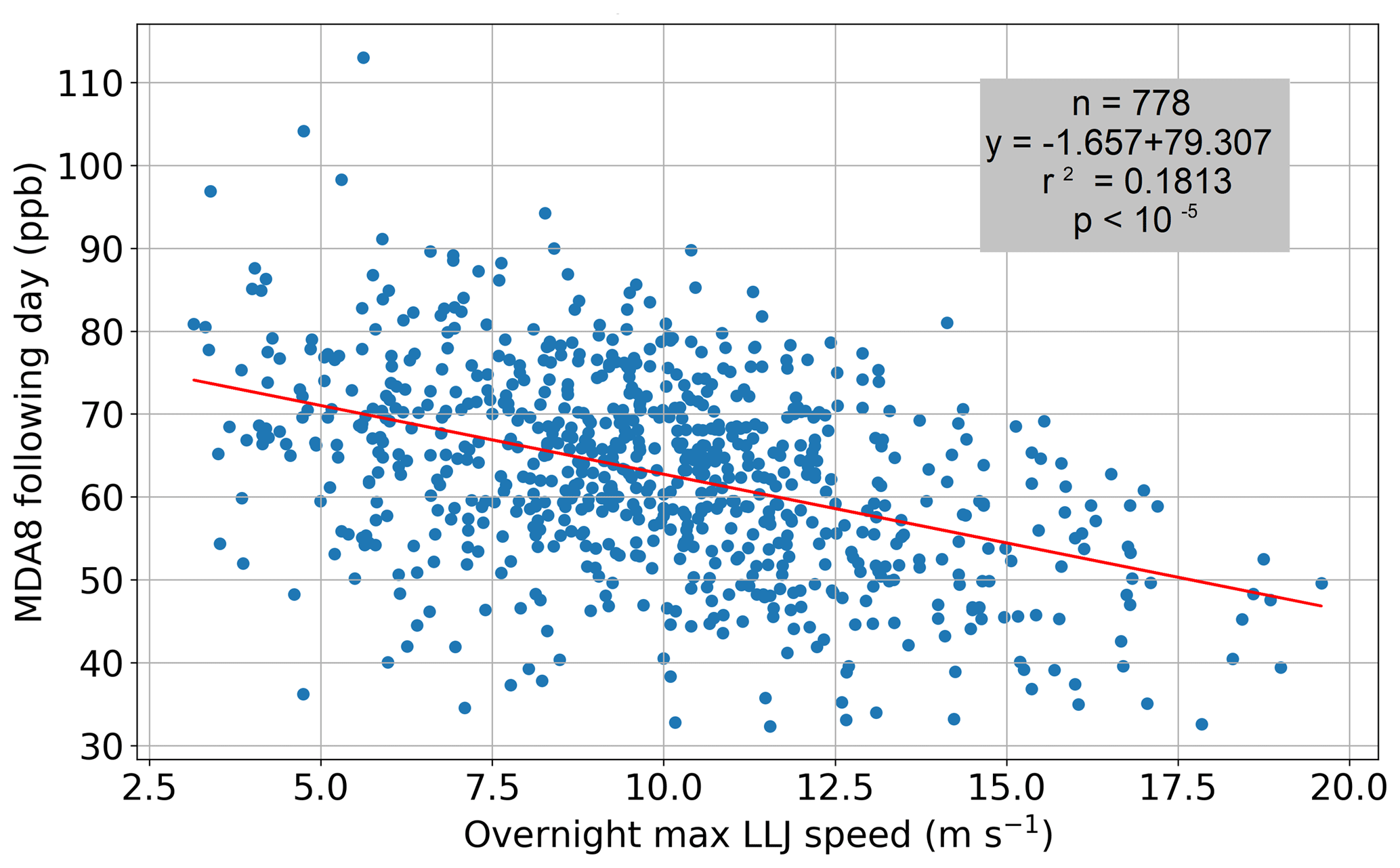
Figure 11Correlation between nocturnal low-level jet speed and the following day's MDA8 in Visalia, CA, for calendar days 152–273 from 2010 to 2016.

Download

The physical processes of RL O_x depletion once it mixes down into the NBL represent a further question. The main destruction processes of O_x in the NBL are chemical loss and dry deposition. One possibility is that surface sources of NO₂ contribute to the excess nocturnal chemical depletion of O_x in the NBL. However, the chemical loss of O_x is not thought to vary significantly between the RL and NBL because the increase in NO₂ in the NBL is compensated for by the decrease in O₃ (see Fig. 4), although this assumes that there are no other chemical differences that alter the reaction fate of nitrate (i.e., α in Eq. 1). Another possibility is that the deposition velocity of ozone may be enhanced by a reduction of aerodynamic resistance under a stronger LLJ. The dry deposition of any gas may be characterized by a series of resistances (Wesely, 1989):

where r_a is the aerodynamic resistance, r_b is the viscous sub-layer resistance, and r_c is the surface (or canopy) resistance. Figure 4 in Padro (1996) suggests that for ozone at night, $r_{\mathrm{a}}\sim r_{\mathrm{c}}\sim \mathrm{250}$ s m⁻¹. r_b is likely nonzero (Massman et al., 1994) but is typically several times smaller than the other resistances (Georgiadis et al., 1995; Pilegaard et al., 1998), so we assume that $r_{\mathrm{a}}=r_{\mathrm{b}}+r_{\mathrm{c}}=\mathrm{250}$ s m⁻¹ to yield our estimated deposition velocity of 0.2 cm s⁻¹. Combining an estimate of aerodynamic resistance due to mass transfer ($r_{\mathrm{a}}=U{u}_{\ast }^{-\mathrm{2}}$, where $u_{\ast }^{\mathrm{2}}$ is the momentum flux) and parameterizing the momentum flux as a function of 10 m wind speed, U₁₀, and a drag coefficient C_D ($u_{\ast }^{\mathrm{2}}=C_{\mathrm{D}}{U}_{\mathrm{10}}^{\mathrm{2}})$, we roughly approximate r_a as

In the 7 years of LLJ data at Visalia, the 10 m wind speed is correlated with the jet strength (r²=0.309, $p<{\mathrm{10}}^{-\mathrm{5}})$. On average, U₁₀ was 1 for 5 m s⁻¹ jets and 2.5 for 15 m s⁻¹ jets. Assuming an average U₁₀ of 1.75 m s⁻¹ and r_a of 250 s m⁻¹, this would imply that $C_{\mathrm{D}}\sim \mathrm{2.3}\times {\mathrm{10}}^{-\mathrm{3}}$. A sensitivity analysis indicates that the difference in U₁₀ between strong and weak jets would result in an approximate 40 % change in v_d. We thus conclude that the LLJ likely plays a significant role in modulating the dry deposition rate, whereby a strong jet decreases r_a and thus increases v_d, further contributing to a loss of ozone overnight. It is important to note that what we have presented is only a rough estimate of the variability of r_a, and thus future studies should measure these parameters with more precision in order to better estimate the degree to which the LLJ can modulate dry deposition in the SJV. The average error of K_z due to the uncertainty in v_d is calculated to be ∼0.50 m² s⁻¹ and is included in our error propagation analysis.

3.5 Eddy diffusivity and other estimates of turbulence

Here we attempt to build confidence in the eddy diffusivity estimates by analyzing additional metrics of turbulence. We find that nocturnally and spatially averaged TKE in the NBL ranges from 0.35 to 1.02 m² s⁻², which is very comparable to values obtained in other NBL studies (Banta et al., 2006; Lenschow et al., 1988). Table 1 shows the TKE, LLJ speed, and the ratio of the streamwise variance to LLJ speed (σ_u∕U_x) for each night. The average value of σ_u∕U_x in this study is 0.11, approximately double what was reported in Banta et al. (2006). There is no detectable relationship between our calculated NBL TKE and eddy diffusivities, LLJ speed, or MDA8 the following day, which implies that the eddy diffusivities calculated from the scalar budget analysis may be a better measure of nocturnal mixing strength than TKE.

Our budget method of estimating turbulent dispersion differs from some other attempts that have been made for stably stratified environments. Clayson and Kantha (2008) applied a technique that had been previously used in oceans to the free troposphere, where turbulence is sparse and intermittent, much like in the NBL. Their method involves using high-resolution soundings to estimate a length scale of overturning eddies, known as the Thorpe scale (Thorpe, 2005), which is then used to obtain estimates of turbulent dissipation rate and subsequently eddy diffusivity. This is done by relating the Thorpe scale to the Ozmidov scale, whereby if the Brunt–Väisälä frequency (N_BV) is known, the TKE dissipation rate (ε) can be estimated. Eddy diffusivity can then be estimated as a product of the TKE dissipation and N⁻²:

where γ is the mixing efficiency, which can vary between 0.2 and 1 (Fukao et al., 1994). From the nocturnal power spectra (Fig. 1) we use a Kolmogorov fit to estimate ε, which is determined to be approximately $\mathrm{4.8}\times {\mathrm{10}}^{-\mathrm{6}}$ m² s⁻³ for the overall altitude range of our nighttime flights (surface to ∼3000 m), but a median of $\mathrm{3.0}\times {\mathrm{10}}^{-\mathrm{4}}$ m² s⁻³ is observed in the NBL. Using the average NBL Brunt–Väisälä frequency of 0.023 Hz, a mixing efficiency of 0.6, and the median NBL ε results in an eddy diffusivity of 0.34 m² s⁻¹, which is about 3 times smaller than the lower end of our range (1.1–3.5 m² s⁻¹). A recent study of vertical mixing based on scalar budgeting of radon-222 in the NBL by Kondo et al. (2014) estimated 7-day average overnight diffusivities of 0.05–0.13 m² s⁻¹, which are an order of magnitude below our estimates inferred from the O_x budget. However, Wilson (2004) conducted a meta-analysis of radar-based estimates of eddy diffusivity in the free troposphere, which is also a generally stable environment, and found a range of 0.3–3 m² s⁻¹. Pisso and Legras (2008) estimated diffusivities of about 0.5 in the lower stratosphere during Rossby-wave-induced intrusions of midlatitude air into the subtropical region. A modeling study by Hegglin et al. (2005) reports diffusivities of 0.45–1.1 m² s⁻¹ in the lower stratosphere with an average Brunt–Väisälä frequency of 0.021 Hz, indicating a similar turbulent environment to ours. Finally, Lenschow et al. (1988) analyzed flight data in the NBL over rolling terrain in Oklahoma and found eddy diffusivities for heat (K_h) of ∼0.25 m² s⁻¹ for the upper half of the NBL and ∼1 m² s⁻¹ for the lower half. To our knowledge, the latter is the most comparable observational finding within the NBL to our range of diffusivities. Nevertheless, the variability in the reported values leads to the conclusion that vertical diffusivity in very stable environments is poorly understood, and further research is necessary to illuminate its phenomenology. More specifically, while it is possible that the diffusivity measurements in this study are biased high (e.g., due to overestimates of the chemical loss parameter α), it is also possible that the LLJ and other mesoscale wind features of the complex terrain account for stronger nocturnal mixing in the SSJV compared to those in other stable environments.

Lastly, we estimate the BRN on each late-night flight within the NBL using 100 m bins to estimate wind shear. A range of Richardson numbers between 0.23 and 1.34 is obtained, and the estimates are seen to have a slight negative relationship with eddy diffusivities as illustrated in Fig. 12. The weak correlation is probably the result of the limited dataset coupled with the challenging nature of both the eddy diffusivity and BRN measurements.

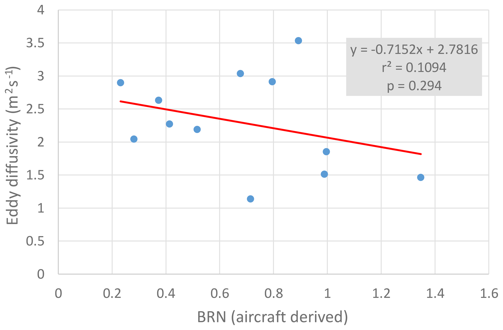
Figure 12Eddy diffusivities and bulk Richardson numbers (BRNs) derived from aircraft observations.

Download

3.6 Nocturnal elevated mixed layers

During the late-night flights in stable environments, the flight crew reported many patches of turbulence. While most of these subjective reports were during low approaches and thus likely attributable to wind shear between the LLJ and the surface, they noted that some patches corresponded to what appeared to be elevated mixed layers, i.e., layers of air in which virtual potential temperature was observed to decrease with height. These layers may be of special interest to our analysis of overnight mixing, since absolutely unstable layers of air generate turbulence and vertical mixing. The time series of all late-night flights was scanned for any period during which (1) the aircraft maintained an ascent (or descent) rate of at least 1.4 m s⁻¹, and (2) during a given elevation span of at least 100 m, a virtual potential temperature decrease with height was observed. The process was repeated for a thickness of at least 50 m.

The locations of the layers greater than 50 m thickness, along with their elevation and lapse rate, are shown in Fig. 13. One feature of note is that the layers appear to be more prominent over urban areas, such as Fresno, Visalia, and Bakersfield. This may lead one to suspect that some of these layers are driven by an urban heating effect; however, this seems unlikely as the unstable layers appear mostly above the NBL wherein the communication with the surface is relatively rapid. Rather, the appearance of these layers clustering around urban areas may be the result of a flight sampling bias and thus may not be significant. Another feature worth noting is that more unstable layers are observed closer to the Tehachapi Pass. One possible explanation for this is that the katabatic flow down the mountain slopes detrains along the way and is carried over the valley by local advection before mixing with surrounding air. Given that these layers are found from near the bottom of the RL all the way up to 2.5 km, it is possible that they contribute to the overnight mixing of O_x from the RL to the NBL by maintaining a fairly well-mixed lower atmosphere over the valley. Further research, both observational and modeling based, is needed to explore this possibility.

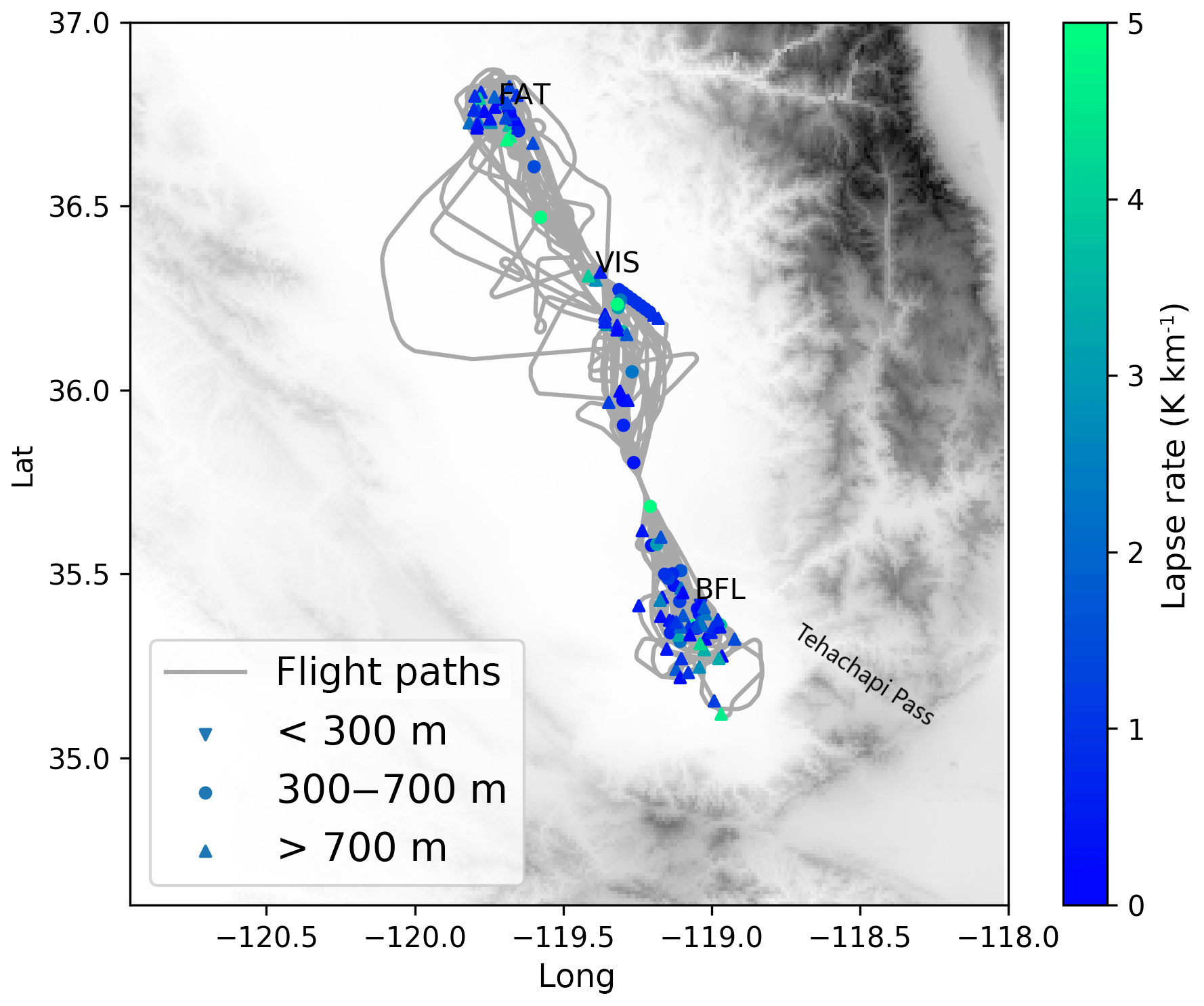
Figure 13Detected nocturnal elevated mixed layers with at least 50 m thickness, with elevations shown.

Download

The unstable layers are not found to have more TKE than the rest of the atmosphere. While this may reflect the limitations of the method used to estimate turbulence from this low-cost wind measurement system, it is consistent with the study by Cho et al. (2003) that found no relationship between turbulence and static stability in the free troposphere. Interestingly, their analysis of aircraft data collected over the Pacific Ocean up to 8 km of altitude found unstable layers in 6 % to 25 % (depending on the layer thickness definition of 100 to 10 m) of their profiles above the boundary layer (Cho et al., 2003). Because the aircraft moves more than 10 times faster horizontally than vertically during profiling, the observations of the elevated mixed layers may be an artifact of localized temperature gradients that are more prominent in the horizontal dimension. To confirm that this is not the case, we examined the wind quivers in the unstable layers along with the direction of the colder air. The cooler air was not systematically detected in any one direction, which supports the hypothesis that they are true vertical temperature gradients.

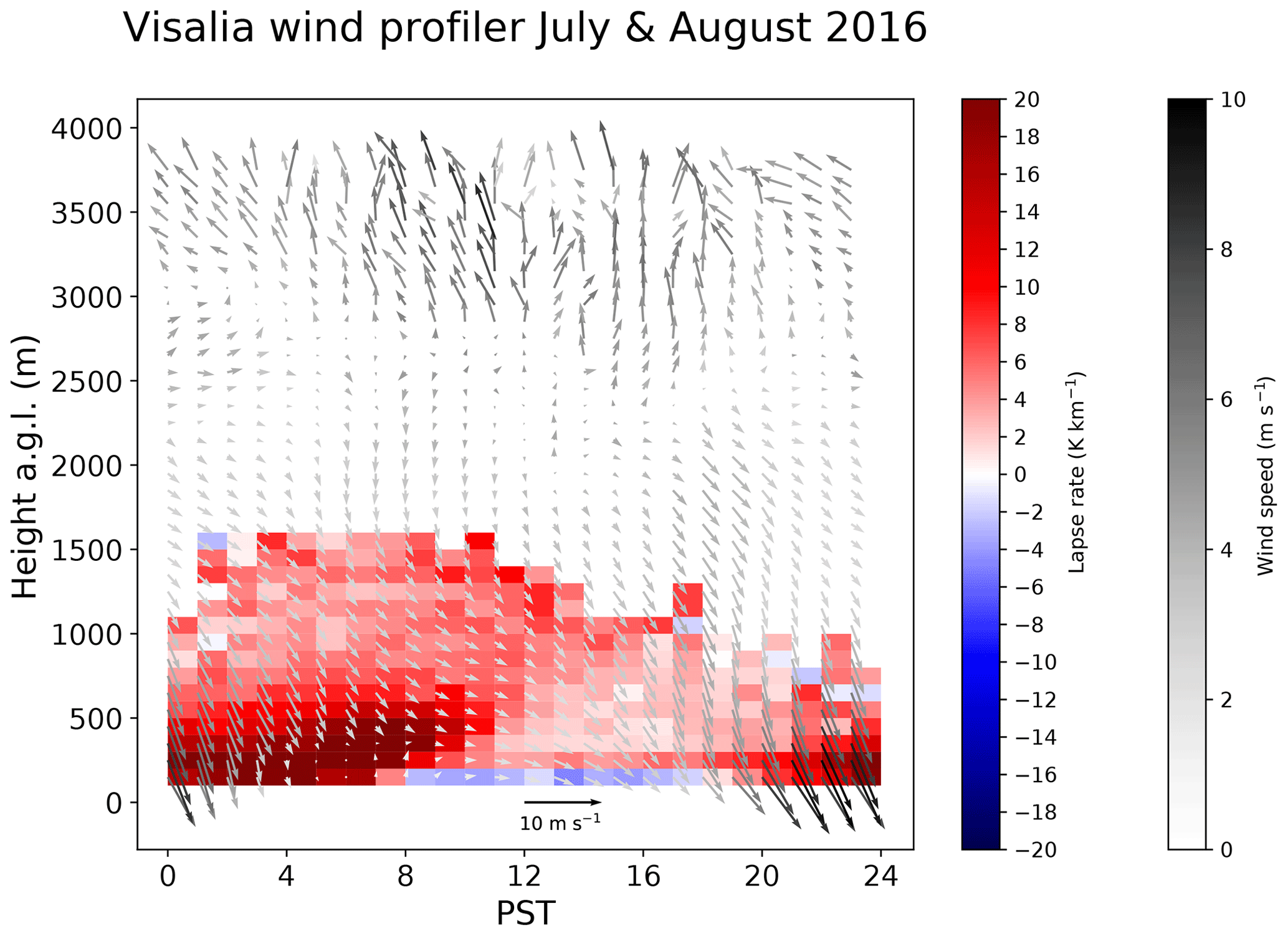
To analyze the stability, wind shear, and turbulence from a climatological standpoint, a July–August 2016 composite of the 915 MHz Visalia sounder data is presented in Fig. 14. Even in the 2-month averages, some nocturnal unstable layers are detectable between 500 and 1500 m, which further supports the existence of persistent elevated mixed layers that may contribute to the overnight mixing of pollutants in the lower troposphere over the valley.

Figure 14Stability and wind quivers for the Visalia 915 MHz sounder, 1 July–31 August 2016.

Download