the Creative Commons Attribution 4.0 License.
the Creative Commons Attribution 4.0 License.
 | 08 Apr 2019
Analysis of atmospheric CH4 in Canadian Arctic and estimation of the regional CH4 fluxes
Douglas Chan
Doug Worthy
Elton Chan
Felix Vogel
Shamil Maksyutov
The Canadian Arctic (> 60∘ N, 60–141∘ W) may undergo drastic changes if the Arctic warming trend continues. For methane (CH4), Arctic reservoirs are large and widespread, and the climate feedbacks from such changes may be potentially substantial. Current bottom-up and top-down estimates of the regional CH4 flux range widely. This study analyzes the recent observations of atmospheric CH4 from five arctic monitoring sites and presents estimates of the regional CH4 fluxes for 2012–2015. The observational data reveal sizeable synoptic summertime enhancements in the atmospheric CH4 that are distinguishable from background variations, which indicate strong regional fluxes (primarily wetland and biomass burning CH4 emissions) around Behchoko and Inuvik in the western Canadian Arctic. Three regional Bayesian inversion modelling systems with two Lagrangian particle dispersion models and three meteorological datasets are applied to estimate fluxes for the Canadian Arctic and show relatively robust results in amplitude and temporal variations across different transport models, prior fluxes, and subregion masking. The estimated mean total CH4 flux for the entire Canadian Arctic is 1.8±0.6 Tg CH4 yr−1. The flux estimate is partitioned into biomass burning of 0.3±0.1 Tg CH4 yr−1 and the remaining natural (wetland) flux of 1.5±0.5 Tg CH4 yr−1. The summer natural CH4 flux estimates clearly show inter-annual variability that is positively correlated with surface temperature anomalies. The results indicate that years with warmer summer conditions result in more wetland CH4 emissions. More data and analysis are required to statistically characterize the dependence of regional CH4 fluxes on the climate in the Arctic. These Arctic measurement sites will aid in quantifying the inter-annual variations and long-term trends in CH4 emissions in the Canadian Arctic.
- Article
(8072 KB) -
Supplement
(1142 KB) - BibTeX
- EndNote


The works published in this journal are distributed under the Creative
Commons Attribution 4.0 License. This license does not affect the Crown copyright work,
which is re-usable under the Open Government Licence (OGL). The Creative Commons Attribution
4.0 License and the OGL are interoperable and do not conflict with, reduce or limit each other.
© Crown copyright 2019
Atmospheric methane (CH4) is one of the principal greenhouse gases with a global warming potential (GWP) 34 times stronger than carbon dioxide (CO2) over a 100-year time period and 96 times stronger over a 20-year time period (Gasser et al., 2017). Atmospheric level of CH4 has doubled since the pre-industrial era, from about 722 to 1803 ppb in 2011 (Ciais et al., 2013). Natural wetland CH4 emission in Arctic regions is of much interest to the scientific community because the CH4 emissions can potentially increase in a warming climate (AMAP, 2015). The Arctic is underlain with continuous permafrost containing large quantities of soil carbon, ∼1700 PgC (Tarnocai et al., 2009). Under warming scenarios, this stored carbon may be highly vulnerable to conversion to CH4 and CO2, which can be emitted to the atmosphere. However, there is only low confidence in the exact magnitude of CO2 and CH4 emissions caused by the permafrost thawing and whether carbon will decompose aerobically to release CO2 or anaerobically to release CH4 (e.g., McGuire et al., 2009; Schuur et al., 2015; Thornton et al., 2016).
Natural CH4 flux estimates are highly uncertain in northern high latitudes. There have been many studies on CH4 emission using both bottom-up and top-down methods. A thorough review of these studies can be found in Saunois et al. (2016). In general, bottom-up flux estimates for the northern high latitudes from biogeochemical CH4 models have large variations, with the mean estimates being much higher than top-down estimates from inverse modelling (Saunois et al., 2016). For the boreal North America region including Alaska and the Hudson Bay Lowlands (HBL, the second largest boreal wetland in the world), the bottom-up mean estimate is ∼32 Tg CH4 yr−1, with a wide range from 15 to 60 Tg CH4 yr−1. Conversely, the top-down mean estimate is ∼12 Tg CH4 yr−1 with a narrower range from ∼7 to 21 Tg CH4 yr−1.
Bottom-up estimates from wetland methane models in WETCHIMP show large discrepancies in the spatial distribution of the wetland CH4 source, as well as its magnitude (Melton et al., 2013). In the higher latitudes, the limited ground-based information has hindered the mapping of wetland area. Recently, remote sensing provided more information, but the high-latitude wetland extent still contains large uncertainties (Olefeldt et al., 2016; Thornton et al., 2016). In addition to uncertainty in wetland extent, other factors affecting high-latitude wetland emissions in different models still remain. In a recent inter-comparison of CH4 wetland models (Poulter et al., 2017), all models used the same wetland extent, Surface Water Microwave Product Series (SWAMPS) (Schroeder et al., 2015) with Global Lakes and Wetland Database (GLWD) (Lehner and Döll, 2004), and the same meteorological data (CRU-NCEP v4.0 reconstructed climate data) to drive their models. The models showed a large range in estimated CH4 emission for the North American boreal–Arctic region, compared to other regions in the world. This large range of the CH4 emissions for the North American boreal–Arctic region clearly shows the uncertainty in our current understanding of the physical and biogeochemical processes that contribute to wetland CH4 emissions.
Top-down atmospheric inverse models have been developed to infer fluxes with observed atmospheric CH4 mixing ratios as constraints. Global CH4 inversion studies estimate global distribution of emissions and sinks from observational sites from around the world (e.g., Bousquet et al., 2011; Bergamaschi et al., 2013; Bruhwiler et al., 2014) but with very limited observational information in northern high latitudes for these studies. Recently ground-based observational coverage in northern high latitudes improved with the expansion of towers and aircraft atmospheric observing platforms in Arctic regions (e. g. Karion et al., 2016; Sasakawa et al., 2010; Chang et at., 2014). These observations have been used for CH4 flux estimation in specific regions. For North America, previous atmospheric CH4 studies were mainly focused on Alaska (e.g., Miller et al., 2016; Hartery et al. 2018). Thompson et al. (2017) conducted CH4 flux estimates for the entire region north of 50∘ N, combining recent high-latitude surface observations. Estimated CH4 emissions for the Canadian Arctic (representing the land region of Canada north of 60∘ N) show discrepancies among the inverse studies; the mean annual total CH4 emission (2006–2010) is ∼1.8 Tg CH4 by TM5-4DVAR (Bergamaschi et al., 2013), 0.5 Tg CH4 by CarbonTracker-CH4 (Bruhwiler et al., 2014), and 2.1 Tg CH4 by FLEXINVERT (Thompson et al., 2017). Differences including model transports, prior fluxes, and observational datasets could affect the inversion results. The previous CH4 inversion studies used only observations from Alert in the Canadian Arctic, the most northern observational site in the world. Several new sites in the Canadian Arctic (described in the next paragraph) might be helpful in constraining flux estimation.
Canada has a vast Arctic and sub-Arctic region (∼39 % of Canada's total land) with wetlands and permafrost. It is important to study the methane cycle and monitor the effects of climate change in this sensitive region as these effects could impact atmospheric CH4 levels at national, continental, and hemispheric scales. Environment and Climate Change Canada (ECCC) has recently added five greenhouse gas (GHG) measurement sites in northern Canada to monitor the time evolution of Arctic GHGs in view of better constraining flux estimates in the region. In October 2010, ECCC started continuous GHG measurements at Behchoko (BCK, 115.9∘ W, 62.8∘ N), the first ground-based site of continuous measurements in the Canadian Arctic other than Alert (ALT, 82.5∘ N, 62.5∘ W) where continuous measurements were implemented in 1988. Following BCK, additional continuous measurement programs were implemented at Churchill (CHL, 58.7∘ N, 93.8∘ W) in 2011, Inuvik (INU, 68.3∘ N, 133.5∘ W) and Cambridge Bay (CBY, 69.1∘ N, 105.1∘ W) in 2012, and Baker Lake (BLK, 64.3∘ N, 96.0∘ W) in 2017.
We present the first study to analyze the atmospheric CH4 mixing ratios from the above new ECCC observational sites located in the Canadian Arctic region. In this study, we address three key questions: (1) what information can these new measurements provide in regards to local and regional sources? (2) What are the estimated CH4 fluxes in the Canadian Arctic using inverse modelling with these new measurements? (3) Are there any relationships between the Canadian Arctic CH4 fluxes and climate–environmental variations? This paper is structured as follows: In Sect. 2, the description of the measurement sites as well as the observational data analyses from daily to inter-annual timescales are given. Section 3 describes the inversion model framework. Section 4 presents flux estimates along with flux uncertainties and potential correlations with climate anomalies.
ECCC operates six measurement sites in the Canadian Arctic region to monitor the GHG mixing ratios. Alert (ALT) is the most northern GHG monitoring site on the globe. Weekly flask samples for CO2 measurements began in 1975. Continuous CH4 measurement started in 1988. The other five Arctic and sub-Arctic sites, Behchoko (BCK), Churchill (CHL), Inuvik (INU), Cambridge Bay (CBY), and Baker Lake (BLK), gradually became operational starting in 2007. BLK is the most recent site in the Canadian Arctic with continuous measurement started in July 2017, which augmented the flask air sampling measurement program (started in 2014). At the four other sites, continuous measurement systems were initiated during the period of 2010–2012. The observations from these four sites were used for the inversion in this study. Further detailed site information of all six measurement sites is in Table 1. A map showing their locations is in Fig. 1. Currently, all ECCC continuous measurements are conducted using an in situ cavity ring-down spectrometer (CRDS, Picarro G1301, G2301, or G2401), and discrete flask air samples are measured using a gas chromatograph equipped with flame ionization detectors (GC-FID, Agilent 6890). Both measurements are traceable to the World Meteorological Organization (WMO) X2004 scale (Dlugokencky et al., 2005). In the following sections, we describe the sites briefly and characterize the observed variations in the CH4 mixing ratios at the sites.
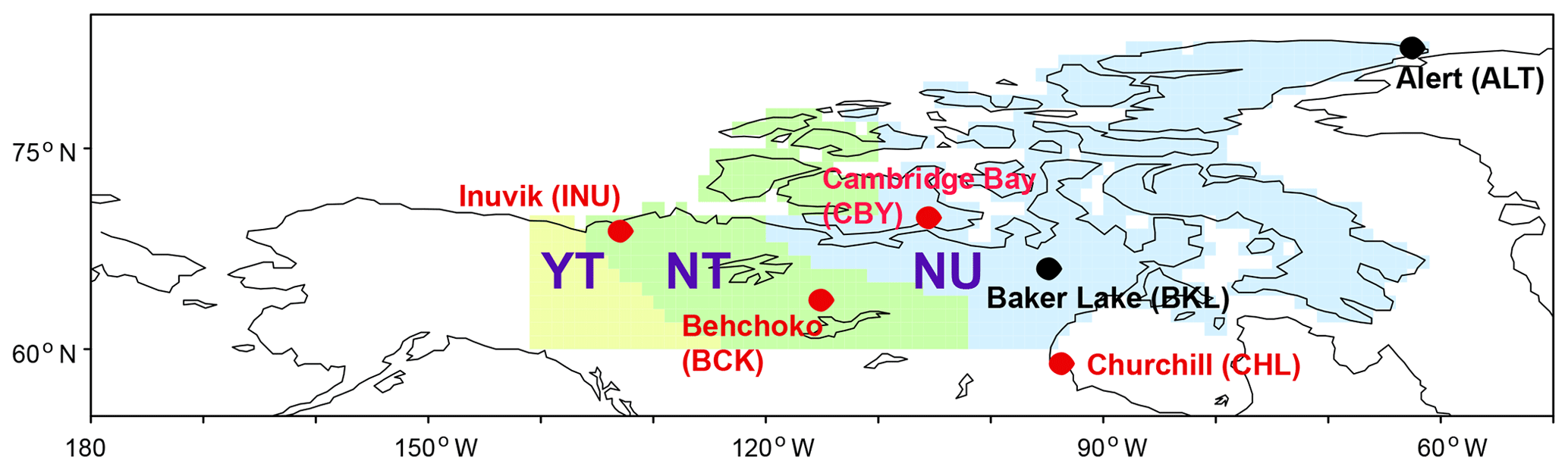
Figure 1The ECCC atmospheric measurement sites around the Arctic. The sites used for the inversion are indicated in red. The three shaded areas are the three territories which are used as subregions in the inversions: YT (Yukon), NT (Northwest Territories), and NU (Nunavut).
Table 1ECCC atmospheric measurement sites in the Canadian Arctic.

* The sites are used in the inversion in this study.
2.1 Site descriptions
Being located thousands of kilometres from major GHG source regions, Alert (ALT, 82.5∘ N, 62.5∘ W) is often referred to as an Arctic background site. The Alert observatory is located ∼6 km away from the main military base camp. The lack of a local source surrounding the site results in no significant diurnal variation in observed atmospheric CH4 mixing ratios throughout the year. In winter, under weak vertical mixing, well-defined synoptic variations are observed due to intercontinental-scale transport along with mainly anthropogenic CH4 originating from the Eurasia continent (Worthy et al., 2009). The measurements at Alert typically represent large-scale background conditions and are thus ideal for providing information on the long-term trend and seasonal cycle for the Arctic (Worthy et al., 2009).
Behchoko (BCK, 62.8∘ N, 115.9∘ W) is located on the northwest tip of Great Slave Lake. The continuous measurement program started in October 2012. Flask sampling is not conducted at this site. The air sampling intake is installed at the top of a 60 m communication tower. The observational equipment is placed in a small isolated room in a local backup power generation station that is rarely turned on. BCK is located 10 km away from the town of Behchoko that is a community ∼80 km northwest of Yellowknife, the capital of the Northwest Territories. Mixed forests, lakes, and ponds surround the BCK site.
Inuvik (INU, 68.3∘ N, 133.5∘ W) is located ∼120 km south of the coast of the Arctic Ocean. The continuous measurement program started in February 2012. Flask sampling began in May 2012. The measurement system is located in the ECCC upper air weather station building, 5 km southeast of the town of Inuvik. INU is ecologically surrounded by Arctic tundra and geologically located in the east channel of the Mackenzie Delta, where a number of water streams and ponds are formed and vast hydrocarbon deposits are found. Although there are proposed developments of natural gas and pipeline projects, most have been on hold.
Cambridge Bay (CBY, 69.1∘ N, 105.1∘ W) is on the southeast coast of Victoria Island. CBY is located ∼1 km north of the town of Cambridge Bay, the largest port of the Arctic Ocean's Northwest Passage. Both continuous and flask sampling measurements started in December 2012. The measurement system is located in the ECCC upper air weather station building.
Baker Lake (BKL, 64.3∘ N, 96.0∘ W) is located on the shore of Baker Lake, ∼320 km inland of Hudson Bay. Weekly flask air sampling started in June 2014, and the continuous measurement program began in July 2017. The air sampling system is located at the ECCC upper air weather station. BCK is in an Arctic tundra region, surrounded by small lakes.
Churchill (CHL, 58.7∘ N, 93.8∘ W) is located on the west coast of Hudson Bay. The GHG monitoring program began with flask air sampling in 2007. The continuous observational program started in October 2011. The sampling equipment is placed in the Churchill Northern Studies Research Facility, ∼23 km east of the town of Churchill. CHL is situated in an area with Arctic tundra to the north and on the northern perimeter of the Hudson Bay Lowlands, the largest contiguous boreal wetland region in North America.
2.2 Temporal variations
Figure 2 shows a time series of CH4 mixing ratios, hourly means, afternoon means (using hourly data from 12:00 to 16:00 local time), and values from flask sampling for each site. The fitted curve and long-term trend were generated using the merged data containing both continuous afternoon means and flask data. The curve-fitting method has two harmonics of 1-year and half-year cycles along with two low- and high-pass digital filters with cut-off periods of 4 months and 24 months respectively (Nakazawa et al., 1997).
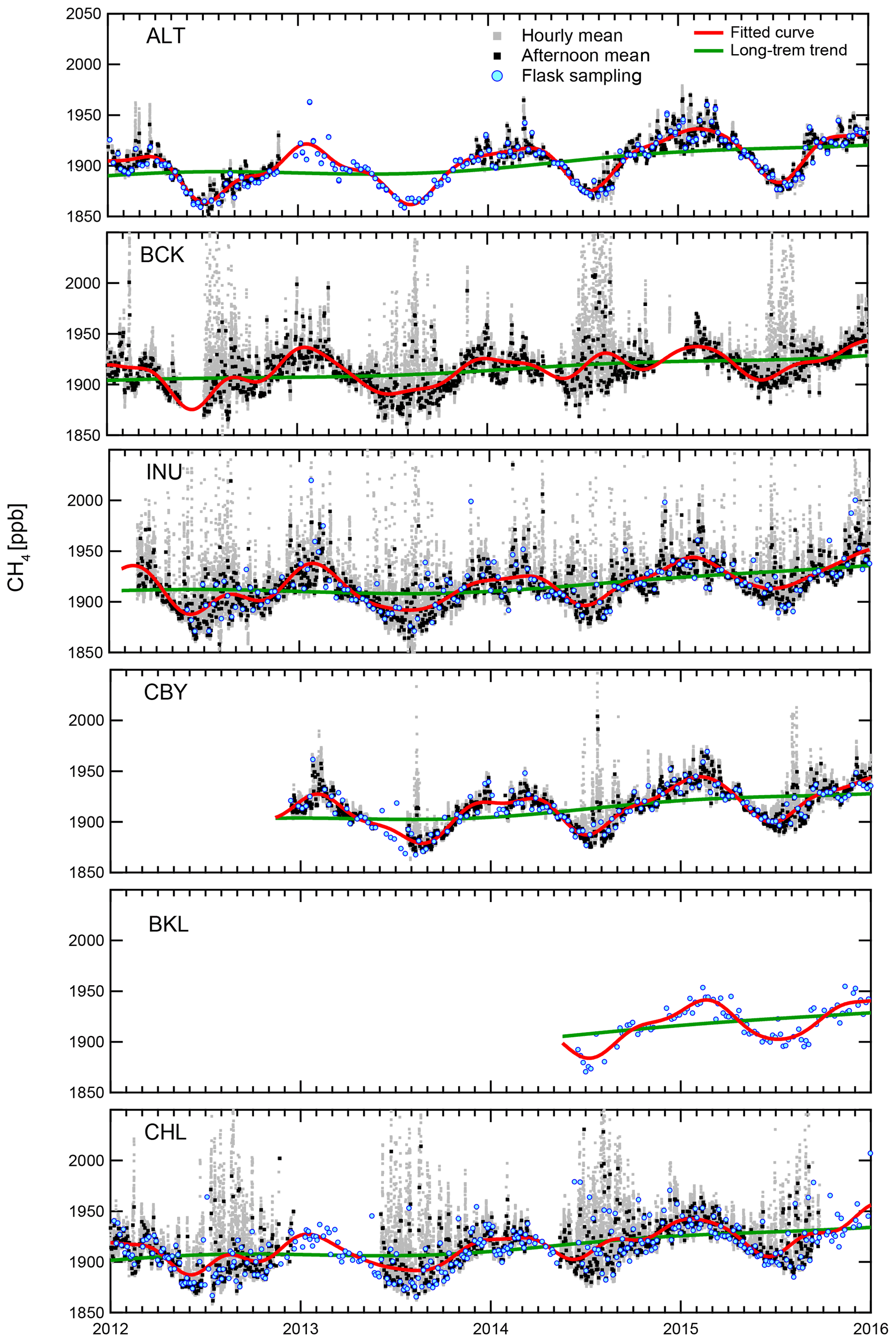
Figure 2Time series of atmospheric CH4 mixing ratios at Canadian Arctic sites. The observed values are the hourly means (grey dot), the afternoon means (black dot, 12:00–16:00 local time) from the continuous measurements, and the ones from flask sampling (circle in light blue). BCK has only continuous measurements. At BKL, flask air sampling is only available after being initiated in 2014. The red and green curves are fitted curves and long-term trends which are obtained by applying a fitting-curve method to the observed afternoon means.
Overall, the features of the continuous and flask measurements show similar long-term trends and seasonal cycles. The continuous measurements reveal short timescale variations that are less visible in the flask data records. The diurnal and synoptic variations in atmospheric CH4 provide information on local- and regional-scale interactions between the atmosphere and the source fluxes (Chan et al., 2004).
All the sites show similar upward trends of atmospheric CH4. The growth rates observed at the Canadian Arctic sites are comparable to the global mean growth rates based on the global network of National Oceanic and Atmospheric Administration (NOAA) air sampling (https://www.esrl.noaa.gov/gmd/ccgg/trends_ch4/, last access: 1 February 2019, Fig. S1 in the Supplement). In 2014, the growth rates jumped at all the sites except BCK. In the following year 2015, the growth rates dropped but were still higher than the growth rates prior to 2014. The rapid enhancement in growth rates at the Canadian Arctic sites is consistent with the globally averaged atmospheric CH4. The year 2014 growth rate at BCK was also enhanced, but the enhancement was not as high as those at the other Arctic sites. This moderate growth rate for BCK might be an artefact in its long-term component partially due to a 2-month period of missing data (mid-November 2014 to mid-January 2015).
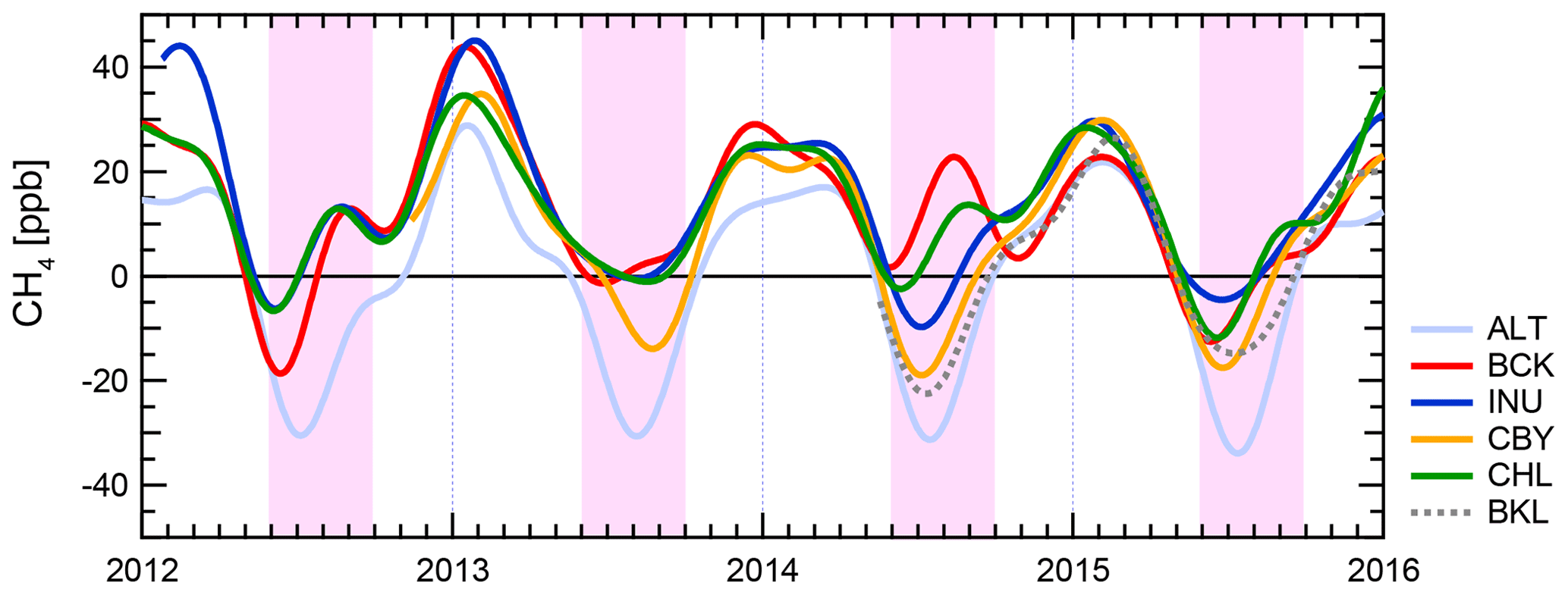
Figure 3Seasonal components in fitted curves of observed atmospheric CH4 mixing ratios at Canadian Arctic sites. Each fitted curve has subtracted the long-term trend component of Alert. Summer months (June-September) are highlighted as light pink shading.
2.2.1 Seasonal and inter-annual variations
Since the long-term trends reflect the global-scale source–sink changes, the long-term component at ALT is subtracted from all the sites in order to isolate the regional-scale signals in the observed atmospheric CH4 data records (Fig. 3). The mean seasonal cycles show a maximum in winter and a minimum in summer. All sites show a similar pattern with a maximum in January–February, while the differences are more noticeable in summer. The summer minimum that is typically representative of the large-scale Arctic background can be seen from July to August at ALT. The summer minima at the other Arctic sites are generally enhanced (with higher CH4 mixing ratios) relative to ALT and very considerably amongst the sites and from year to year. These enhancements and inter-annual variability are due to the superposition of the enhanced atmospheric CH4 sink and increased wetland emissions during warm seasons. Minima are seen in June at BCK, INU, and CHL, followed by BKL and CBY with ∼1- to 1.5-month lags. Another interesting feature seen at INU, BCK, and CHL is a secondary maximum in summer (a summer bump), also indicative of the influence of local and regional wetland and biomass burning emissions. As seen in Fig. 3, these secondary maxima summer bumps vary in timing and amplitude from year to year. The bumps were observed at BCK, INU, and CHL in 2012, which were in phase with each other, but not at any site in 2013. In 2014, a more substantial summer bump was observed at BCK than 2012 (2014 has strong biomass burning contributions) while the summer bump at CHL was similar to the one in 2012. The cause(s) for the summer bumps at BCK, CHL, and INU might vary year to year, such as local–regional (wetland and forest fires) emission change due to climate anomaly. Another possible cause is inter-annually varying atmospheric transport.
2.2.2 Synoptic and diurnal variability
All measurements of atmospheric CH4 in the Canadian Arctic show synoptic and daily variations with seasonally changing amplitudes. One quantitative measure of synoptic variability in the observed CH4 mixing ratios is the monthly standard deviation (SD) of the residual of observed time series relative to their fitted curves. Figure 4 shows the mean seasonality in SD of all 24 hourly data (SD_24) in CH4 mixing ratios at each site except BKL, as well as the mean seasonality of the afternoon hourly data (SD_PM). Although SD_24 and SD_PM appear similar (some are almost identical) except during summer months, the differences between SD_PM and SD_24 provide a measure of whether the daily variability is reflecting a local-scale change in emission or rather a change in the atmospheric transport processes. The nighttime planetary boundary layer (PBL) is usually shallow, while the daytime boundary layer is usually deeper and well mixed. If there are local CH4 sources, the emission will be mixed into a shallow PBL at night (yielding a higher mixing ratio) and diluted through a deeper PBL during the day (yielding a lower mixing ratio). The resultant diurnal variations in the CH4 mixing ratios are evident as larger CH4 SD_24 compared to SD_PM. In the absence of local sources, SD_24 is comparable to SD_PM.
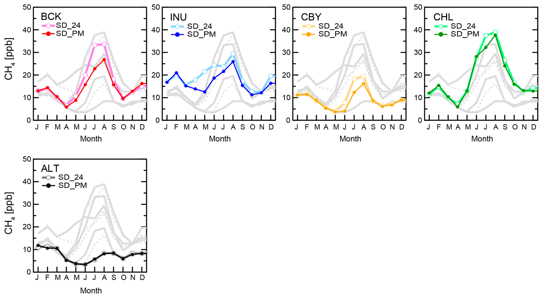
Figure 4Mean seasonal cycles of monthly standard deviation (SD) of observed CH4 mixing ratios, SD_24 of all 24-hourly data (closed circles), and SD_PM of afternoon data (12:00–16:00 local time, open circles) to the fitted curves. For BCK, 2014 data have been excluded from the analysis because of high variability due to massive forest fires around the site.
The most substantial synoptic variations are observed in summer at all sites except ALT (Fig. 4). This indicates that the major regional CH4 emissions in the continental Canadian Arctic occur in summer. At ALT, the largest synoptic variations are observed in winter. The winter synoptic variations are mainly due to strong long-range transport from other regions, which has been demonstrated for ALT (Worthy et al., 2009).
The diurnal variability of atmospheric CH4 is mainly caused by a local CH4 emission signal modulated by daily PBL development or a temporal change in the local source. In summer, the SD_24 values are higher by > 5 ppb than the SD_PM except for ALT. The larger SD_24 in summer supports the existence of local CH4 sources around the sites, likely wetland CH4 emissions. In contrast, the fact ALT has identical SD_24 and SD_PM all year round confirms that there is no significant local source near the site.
Similar to the three continental sites (BCK, INU, CHL), CBY also shows the maxima of SD_24 and SD_PM in summer, but they remain lower than BCK, INU, and CHL but higher than ALT. This indicates that there is a weaker local source of CH4 around CBY than around the three continental sites. In the cold season (September to May), the SD_24 and SD_PM at CBY are almost identical to ALT. It is noticeable that the SD_24 and SD_PM at BCK, INU, and CHL are still higher than ALT until December. These higher SD_24 and SD_PM values in the first half of the cold season might indicate possible CH4 emissions from the ground. Zona et al. (2016) suggested that there are ongoing CH4 emissions from the Alaskan Arctic tundra during the “zero curtain“ period when the soil temperature is near zero with average air temperature below 0 ∘C until the surface is completely frozen.
The SD_24 and SD_PM for winter to spring (January to May) at INU remain higher than the other sites. Also, SD_24 at INU becomes higher than SD_PM from April and remains higher over summer. At the other sites, the difference between SD_24 and SD_PM is seen mainly in the summer months (June–August). This higher variability in atmospheric CH4 at INU in winter and spring, when the surrounding wetland ecosystem is inactive, likely indicates strong local CH4 sources, such as anthropogenic CH4 emissions from natural gas well/refinery facilities. During winter, such local CH4 signals are amplified by the seasonally calm condition (the mean seasonal cycles of wind speed are shown in Fig. S2) and by reduced vertical mixing within the shallow PBL due to the shorter period of daylight in the polar region. Figure S3 shows the deviations (from the fitted curve) of observed hourly and afternoon mean CH4 at INU and BCK along with wind speed. In April and May, the difference in deviations between hourly CH4 and afternoon mean CH4 becomes larger again after the relatively quiet period. This may indicate the signals of local (anthropogenic) emission around INU being amplified as the PBL diurnal variation starts developing due to longer daytime periods. Another possible local source for the large spring SD_24 and SD_PM at INU may be the natural CH4 emissions originating from lakes and ponds during the spring thaw (Jammet et al., 2015). In contrast, SD_24 and SD_PM at BCK become smaller as the wind speed increases, indicating a lack of local CH4 source around BCK in spring.
Since ALT is representative of the Arctic background state in synoptic variability, the difference in SD_24 or SD_PM between ALT and each of the other sites gives a measure of the regional source influence to the site. The sizeable regional source influence signals in summer shown in Fig. 4 should be useful in constraining the regional flux estimation modelling in the next sections.
To estimate the regional CH4 fluxes in the Canadian Arctic, we apply a Bayesian inversion approach, based on the backward simulations by Lagrangian particle dispersion models (LPDMs). In this study, three different transport models and three prior CH4 flux distributions were used to help estimate the model uncertainties. The following sections describe the various components of our regional inverse modelling.
3.1 Transport models and meteorological data
LPDMs simulate an ensemble of air-following particles which are released from the measurement sites. The air particles travel backwards in time for 5 days with the wind field. Previous studies (e.g., Cooper et al., 2010; Gloor et al., 2001; Stohl et al., 2009) have shown 5 days is typically sufficient to capture the surface influence on a measurement site from the surrounding region. The backward trajectories are used to calculate the footprints as the integrated residence times the particles spent inside the PBL at a resolution of . We use three different regional model setups combining two different LPDMs, FLEXPART and STILT, and three different meteorological data from the European Centre for Medium-range Weather Forecasts (ECMWF), Japanese Meteorological Agency (JMA), and Weather Research and Forecasting (WRF) model.
LPDMs simulate local contributions for 5 days prior to the measurements at sites. The background condition of atmospheric CH4 mixing ratios at the endpoints of the particles is provided by a global model, National Institute for Environmental Studies Transport Model (NIES TM) with global CH4 flux fields. Below are the details of model setups in this study.
3.1.1 LPDM: FLEXPART_EI
The first model setup is FLEXible PARTicle dispersion model (FLEXPART) (Stohl et al., 2005) driven by reanalysis meteorology from the European Centre for Medium-range Weather Forecasts (ECMWF) ERA-Interim (Dee et al., 2011; Uppala et al., 2005). The input meteorological data are at 3-hourly time steps and interpolated to horizontal resolution with 62 vertical layers.
3.1.2 LPDM: FLEXPART_JRA55
The second model setup is also FLEXPART, but driven by the Japanese 55-year Reanalysis (JRA-55) from Japanese Meteorological Agency (JMA; Kobayashi et al., 2015; Harada et al., 2016). JRA-55 is at 6-hourly time steps and TL319 (∼0.5625∘, ∼55 km) horizontal resolution with 60 vertical layers. For this study, we use the JRA-55 dataset at the lower resolution (∼1.25∘). This model setup was used for a global inverse modelling system by the Global Eulerian-Lagrangian Coupled Atmospheric Model (GELCA) that is a coupled atmospheric model of NIES TM and FLEXPART (Ishizawa et al., 2016). The primary meteorological observational data for JRA-55 have been supplied by ECMWF. In addition to the ECMWF data, the observational data obtained by JMA and other sources are also used.
3.1.3 LPDM:WRF-STILT
The third model setup uses the Stochastic, Time-Inverted, Lagrangian Transport Model (STILT) (Lin et al., 2003; Lin and Gerbig, 2005). The wind fields to drive STILT are from the Weather Research and Forecasting (WRF) model (Skamarock et al., 2008) at 10 km resolution. Detailed descriptions are found elsewhere (Hu et al., 2019; Miller et al., 2014; Henderson et al., 2015). The footprints are aggregated to horizontal resolution, similar to the other models in this study. The STILT footprint data are provided from CarbonTracker-Lagrange, which is a Lagrangian assimilation framework developed at the NOAA Earth System Research Laboratory (https://www.esrl.noaa.gov/gmd/ccgg/carbontracker-lagrange/, last access: 1 February 2019).
3.1.4 Global background model: NIES TM
The background or initial condition for the LPDMs is obtained by sampling a global model of CH4 at the 5-day back endpoint locations of the LPDM particles. The global background field of the CH4 mixing ratio is simulated by NIES TM version 8.1i (Belikov et al., 2013) with the optimized CH4 fluxes with the GELCA-CH4 inversion system (Ishizawa et al., 2016; Saunois et al., 2016). The GELCA-CH4 inverse modelling system optimized the monthly CH4 fluxes for 2000–2015 to assimilate a global network of surface CH4 measurements available through the GAW World Data Centre for Greenhouse Gases (WDCGG, http://ds.data.jma.go.jp/gmd/wdcgg, last access: 1 February 2019). The prior CH4 fluxes for the GELCA-CH4 global inversion are also used for the regional inversion in this study as described in the later section. The NIES TM has horizontal resolution and 32 vertical layers, driven by JRA-55. For the global simulation, the CH4 loss in the atmosphere is included; the stratospheric CH4 loss and OH oxidation schemes are adapted from a model inter-comparison project “TransCom-CH4” (Patra et al., 2011).
3.2 Prior fluxes
Three cases of prior emissions, labelled as VIS, GEL, and WetC, are used as listed in Table 2. Since the global background atmospheric CH4 field was calculated with GELCA-CH4 inversion posterior fluxes, we chose the prior (VIS) and posterior (GEL) fluxes from GELCA as two cases of prior fluxes in our regional inversion. Note that the continuous CH4 mixing ratio data from the new Canadian Arctic sites were not used in the GELCA-CH4 inversion. In this study, the mean wetland fluxes for the last 5 years of the GELCA global model were used, and the prior forest fire CH4 fluxes are detailed in Sect. 3.2.2. The third prior case (WetC) is the same as GEL but with wetland CH4 fluxes from WetCHARTs (a recent global wetland methane emission model ensemble for use in atmospheric chemical transport models). WetCHARTs provides inter-annually varying monthly wetland CH4 fluxes for this study period. The details of prior fluxes are described in the following sections.
Table 2Three cases of prior CH4 fluxes.
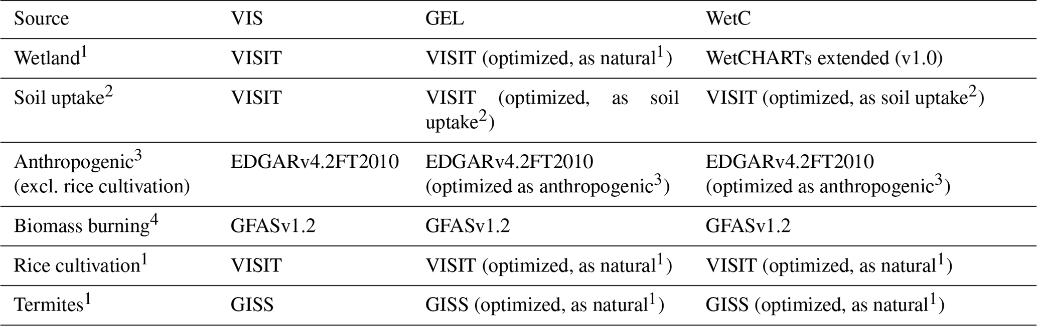
VIS used the same prior fluxes with those for global GELCA-CH4 inversion except biomass burning. GELCA-CH4 inversion optimized CH4 fluxes for four source types: 1 natural, 2 soil uptake, 3 anthropogenic, and 4 biomass burning, which are also indicated by superscripted numbers. GEL used the posterior fluxes from global GELCA-CH4 inversion. For VIS and GEL, the 5-year mean of each source type was used. WetC used WetCHARTs extended mean fluxes as wetland CH4, while other fluxes were the same as GEL. For all the scenarios, GFAS v1.2 daily fluxes were used as biomass burning.
3.2.1 Wetland CH4 fluxes
We used the monthly CH4 wetland fluxes from two different models. The first model is the Vegetation Integrative Simulator for Trace gases (VISIT) (Ito and Inatomi, 2012). VISIT is a process-based model, using GLWD as wetland extent. In addition to wetland CH4 flux, VISIT calculates soil CH4 uptake and CH4 emission through rice cultivation. The wetland fluxes combined with CH4 fluxes from rice cultivation were optimized through the GELCA-CH4 global inversion as a natural CH4 flux. The second model is WetCHARTs 1.0 (Bloom et al., 2017a). WetCHARTs derives wetland CH4 fluxes as a function of a global scaling factor, wetland extent, carbon heterotrophic respiration, and temperature dependence (Bloom et al., 2017b). We used the ensemble mean fluxes over 18 model sets which are available for 2001–2015, using (1) three global scaling factors, (2) two wetland extents, GLWD and GLOBCOVER, (3) CARDAMOM (the global CARbon Data MOdel fraMework) as terrestrial carbon analysis, and (4) three temperature-dependent CH4 respiration functions. The WetCHARTs horizontal resolution is . The modelled CH4 fluxes are aggregated into for this study. Figure 5 shows the spatial distribution of three wetland CH4 fluxes for the summer months (July–August). Overall, they are similar, while WetCHARTs (WetC) has stronger emissions in Northwest Territories than the two wetland fluxes from VIS and GEL, which are based on VISIT.
3.2.2 Forest fire CH4 fluxes
GFAS (Global Fire Assimilation System) v1.2 (Kaiser et al., 2012) provides biomass burning (BB) emissions by assimilating fire radiative power (FRP) from the Moderate Resolution Imaging Spectrometer (MODIS). The FRP observations are firstly corrected for data gaps and then linked to dry matter combustion rates with CH4 emission factors. GFAS has a daily temporal resolution and horizontal resolution. In this study, the daily fire CH4 emissions are spatially aggregated into resolution for the regional inversion, though monthly fluxes were used for the GELCA global inversion.
3.2.3 Anthropogenic emission
The anthropogenic CH4 emissions are provided by EDGAR (Emission Database for Global Atmospheric Research) v4.2FT2010 (http://edgar.jrc.ec.europa.eu, last access: 1 August 2018), except for rice cultivation. EDGARv4.2FT2010 emission, which is originally at resolution, is aggregated into . Since the EDGARv4.2FT2010 data are available until 2010, the same values for 2010 are used for the years beyond 2010. The CH4 emission from rice cultivation was replaced with the one from VISIT-CH4 and then treated as a part of natural fluxes. Since there is no rice field in the Canadian Arctic and the rest of the North American Arctic–boreal region, the influence of CH4 emission from rice cultivation in the region of interest in this study is negligible. The difference in the optimized anthropogenic emissions in the Canadian Arctic from the prior by the global GELCA inversion is almost negligible (from 0.0247 to 0.0250 Tg CH4 yr−1). Compared to the wetland emissions, the anthropogenic emissions are substantially smaller and localized (see Fig. 5).
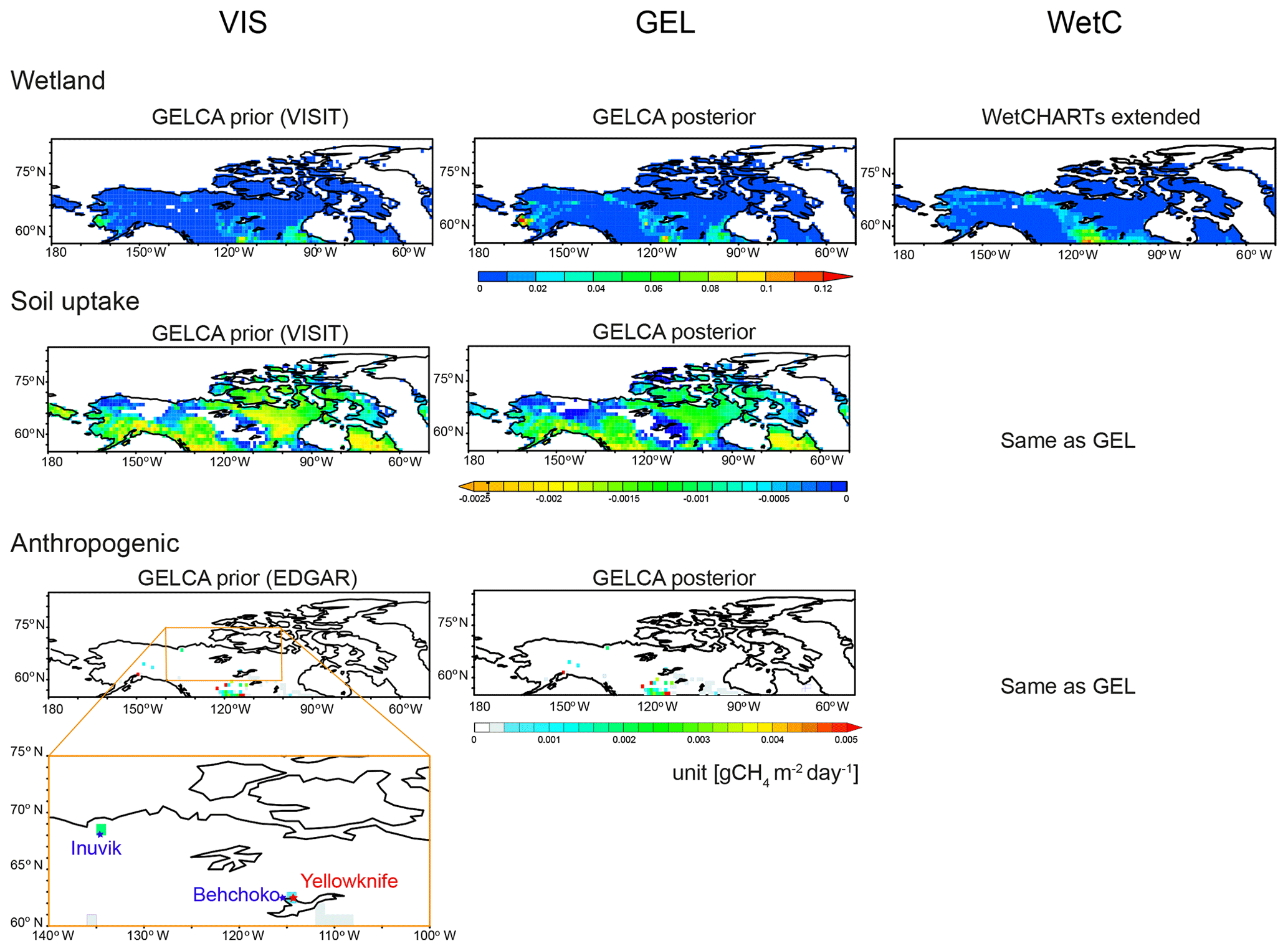
Figure 5Spatial distributions of summertime prior CH4 fluxes of wetland emission, soil uptake, and anthropogenic emissions for the three cases of prior fluxes, VIS, GEL, and WetC, which are listed in Table 2. The bottom left panel is a zoomed anthropogenic emission distribution in Northwest Territories. The locations of two sites, Behchoko (BCK) and Inuvik (INU), and the capital city, Yellowknife, are also plotted.
3.2.4 Other natural CH4 fluxes
For other natural CH4 fluxes, we use a map of climatological termite emissions from Fung et al. (1991) and modelled soil uptake from VISIT-CH4. Because of no termite CH4 emissions in the Canadian Arctic, termite CH4 emission has no direct impact but it is included in global simulation for the background CH4 mixing ratio. The prior soil CH4 uptake is provided by VISIT-CH4 as oxidative consumption by methanotrophic bacteria in unsaturated lands. Soil CH4 uptake has large uncertainty regionally and also globally. Kirschke et al. (2013) reported that global soil uptake ranges from 9 to 47 Tg CH4 yr−1. In the Canadian Arctic, the VISIT-modelled soil uptake is weak (0.094 Tg CH4 yr−1) but spread widely (Fig. 5). In some parts of the eastern Canadian Arctic, soil uptakes exceed other CH4 emissions, resulting in negative fluxes/net sink of atmospheric CH4.
3.3 Inversion setup
3.3.1 Regional inversion
In this study, we use the Bayesian inversion approach (Tarantola, 1987; Rodgers, 2000; Enting, 2002). The Bayesian inversion used here optimizes the scaling factors of posterior fluxes by minimizing the mismatch between modelled and observed mixing ratios with constraints and given uncertainties using the cost function (J) minimization method.
where y (N×1) is the vector of observations (with the background mixing ratio subtracted; see Sect. 3.1.4). N is the number of time points multiplied by number of stations (N is reduced if observations are missing). λ (R×1) is the vector of the posterior scaling factors to be estimated; R is the number of fluxes to be solved. R is two fluxes per subregions × number of subregions (i.e., two to six in this study). λprior is the vector of the prior scaling factors, which are all initialized to 1 for all subregions, and K (N×R) is the matrix of contributions on the observations (N) from all the fluxes (R) of subregions. K is a product of two matrices, M(N×LL) and x (LL×R), M is the modelled transport (or footprints in this study), and x is the spatial distribution of the surface fluxes. LL (lat × long) is the dimension of our domain ( in latitude by longitude). A linear regularization term has been added which is the second term on the right-hand side of the equation. Dϵ and Dprior are the error covariance matrices. Dϵ is the prior model–observation error/uncertainty matrix (N×N), where the diagonal elements are . Dprior is the prior scaling factor uncertainty matrix (R×R), where the diagonal elements are . We assume that the model–observation mismatch errors are uncorrelated with each other and the contributions from the subregions are uncorrelated. All the off-diagonal elements in Dϵ and Dprior are assumed to be zero. We assigned σe=0.33 for the model–observation error (Gerbig et al., 2013; Lin et al., 2004; Zhao et al., 2009) and σprior=0.30 for the prior uncertainty (Zhao et al., 2009). We examined the inversion's sensitivity to these uncertainties by doubling their values. The posterior fluxes changed by less than 5 % for all subregions (and the different subregion masks). The results showed the optimized fluxes are not strongly dependent on these prescribed uncertainties. The estimate for λ is calculated according to the expression below.
The posterior error variance and covariance, Σpost, for the estimates of λ is calculated,
We optimize the CH4 flux from biomass burning and separately optimize the remainder flux (consisting of wetland emission, soil uptake, and anthropogenic emission) per subregion at a monthly time resolution.
3.3.2 Domain/subregions
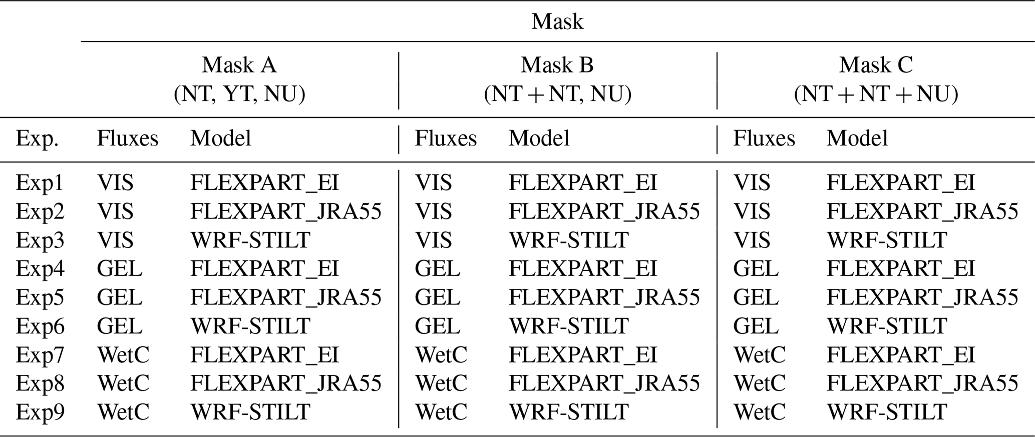
For the Canadian Arctic, which consists of three territories, Northwest Territories (NT), Yukon (YT), and Nunavut (NU), we set up three subregion masks, masks A, B, and C, as shown in Fig. S4. Outside of the Canadian Arctic is treated as one outer region. Regarding the subdivision of the Arctic region, we examined the sensitivity of the flux estimation to the number of subregions. As a starting point, the three territories are treated separately (mask A). Secondly, YT is combined with NT (mask B). There is no existing measurement site in Yukon and no significant CH4 emissions in prior fluxes. The inversion results in the next section will show that YT could not be reliably constrained as a separate subregion (model uncertainties made the estimated fluxes in YT fluctuate from positive to negative). As the third region mask, we solve the fluxes for one region of the entire Canadian Arctic (mask C). Like YT, NU is a weak source region, compared to NT, and weak observational constraint might lead to unrealistic flux estimates. This exercise on the subdivision gives insights into the constraining power of the existing measurements. Table 3 shows all the inversion experiments in this study. We perform 27 experiments in total with three prior emission cases, three different transport models, and three different subregion masks.
Table 3Experiment configurations. Using each of three different masks (A, B, and C in Fig. S3), nine inversion runs were conducted with a combination of three prior flux cases (VIS, GEL, and WetC on Table 2) and three different models (FLEXPART_EI, FLEXPART_JRA55, and WRF-STILT). In total 27 inversion runs were conducted.
3.3.3 Atmospheric measurements
This regional inversion study used the continuous measurements at BCK, INU, CBY, and CHL for 2012–2015 (Fig. 2). First, the afternoon mean values are calculated by averaging the hourly data over 4 h from 12:00 to 16:00 local time so that the observations we use in this study are more regionally representative assuming midday is in a well-mixed planetary boundary layer. Second, the modelled background mixing ratios, which were described in Sect. 3.1.4, are subtracted from the afternoon mean observations. The differences in mixing ratio between observations and background were input into the regional inversion system as local contributions. The observational data examined in Sect. 2 have already been pre-screened for possible contaminations due to mechanical/technical problems during sampling or analyzing processes. Except for the pre-screening, we did not apply any additional data screening or filtering.
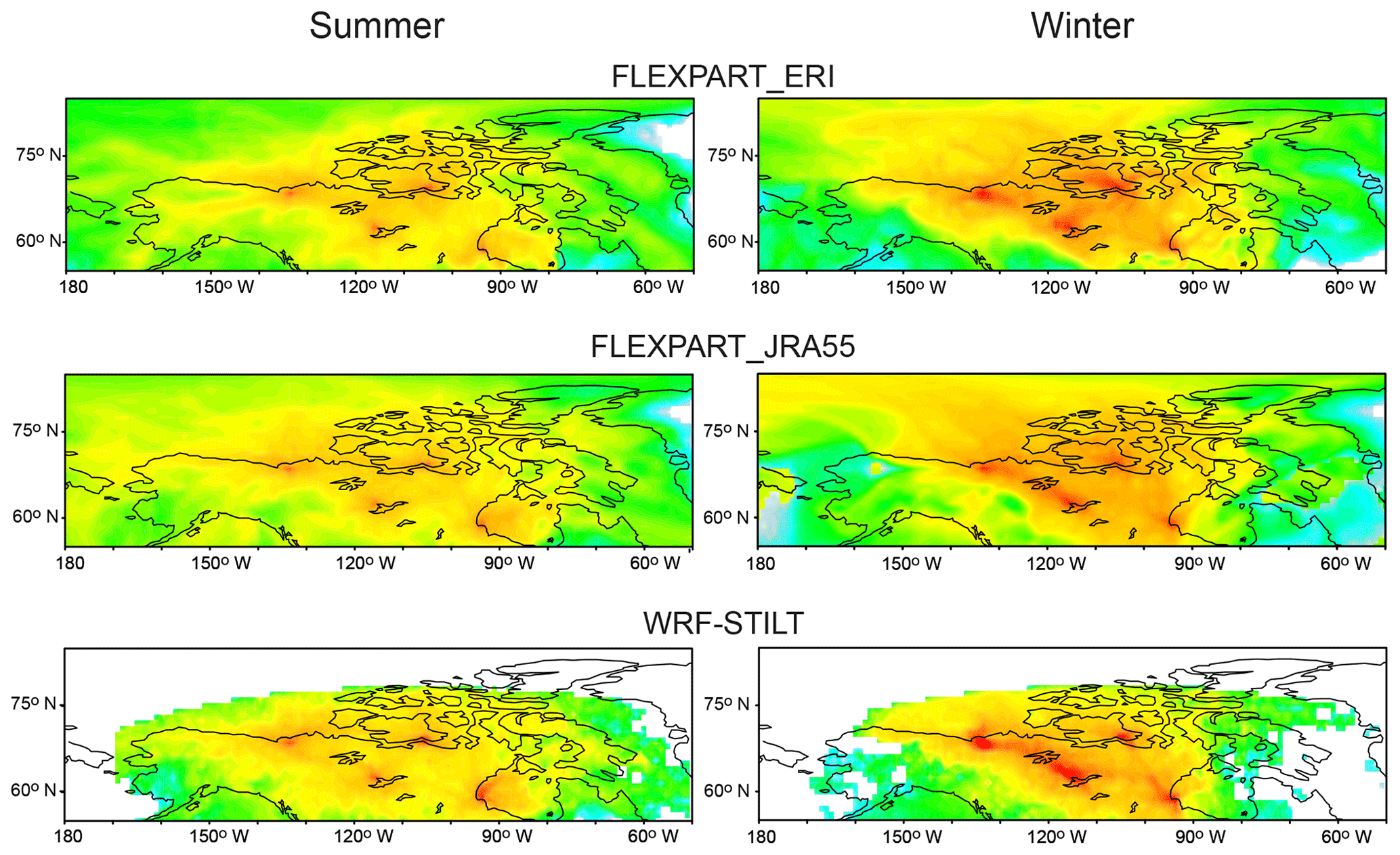
Figure 6Seasonal mean footprints of all sites by three models, shown for summer (July–August 2013) and winter (January–February 2013).
4.1 Comparison of footprints
Figure 6 shows the mean footprints (mean emission sensitivities) of all four sites by the three different LPDMs. There are common features, but there are also noticeable seasonal differences and differences between the models. The spatial coverage is similar, but the sensitivity to emissions around sites depends on the models. Among the models, STILT shows the strongest sensitivity near the sites, while FLEXPART_JRA55 has the weakest sensitivity. All the footprints near the sites for the winter season are stronger than the summer season. The footprint differences among the models are also significant. STILT appears to be more localized around the sites. These differences indicate that choosing multiple implementations for the atmospheric transport will allow us to reflect some of the uncertainties introduced to our inversion estimate by transport models.
4.2 Signals in the observations (relative to background)
The regional inversion depends on how well local signals can be detected in the observations. Therefore, we first look at the detectability of local and regional fluxes in the observed atmospheric CH4 mixing ratios. If the amplitude of local signals is comparable to the background contribution, estimated regional fluxes would be more uncertain because local signals would be difficult to distinguish from the background contributions. In Sect. 2.2.2, we examined the synoptic variability in observed CH4. Here we apply the same procedures to the modelled background CH4 for the sites to see if the local synoptic signal is distinguishable from the background CH4. Figure 7 shows the mean monthly SD of modelled background CH4 to their fitted curves for the case of FLEXPART_EI (other model setups are analogous), along with those of observed CH4 (SD_PM in Fig. 4) for the four sites to be used as observational constraints (BCK, INU, CBY and CHL). In summer, all the SD_PM values of the observations are much larger (up to 3 times) than the respective background SDs, indicating strong local influence. However, in winter, both the observation SD_PM and the background SD are comparable. Thus, the observations could provide more constraints on the estimated regional fluxes in summer than in winter.
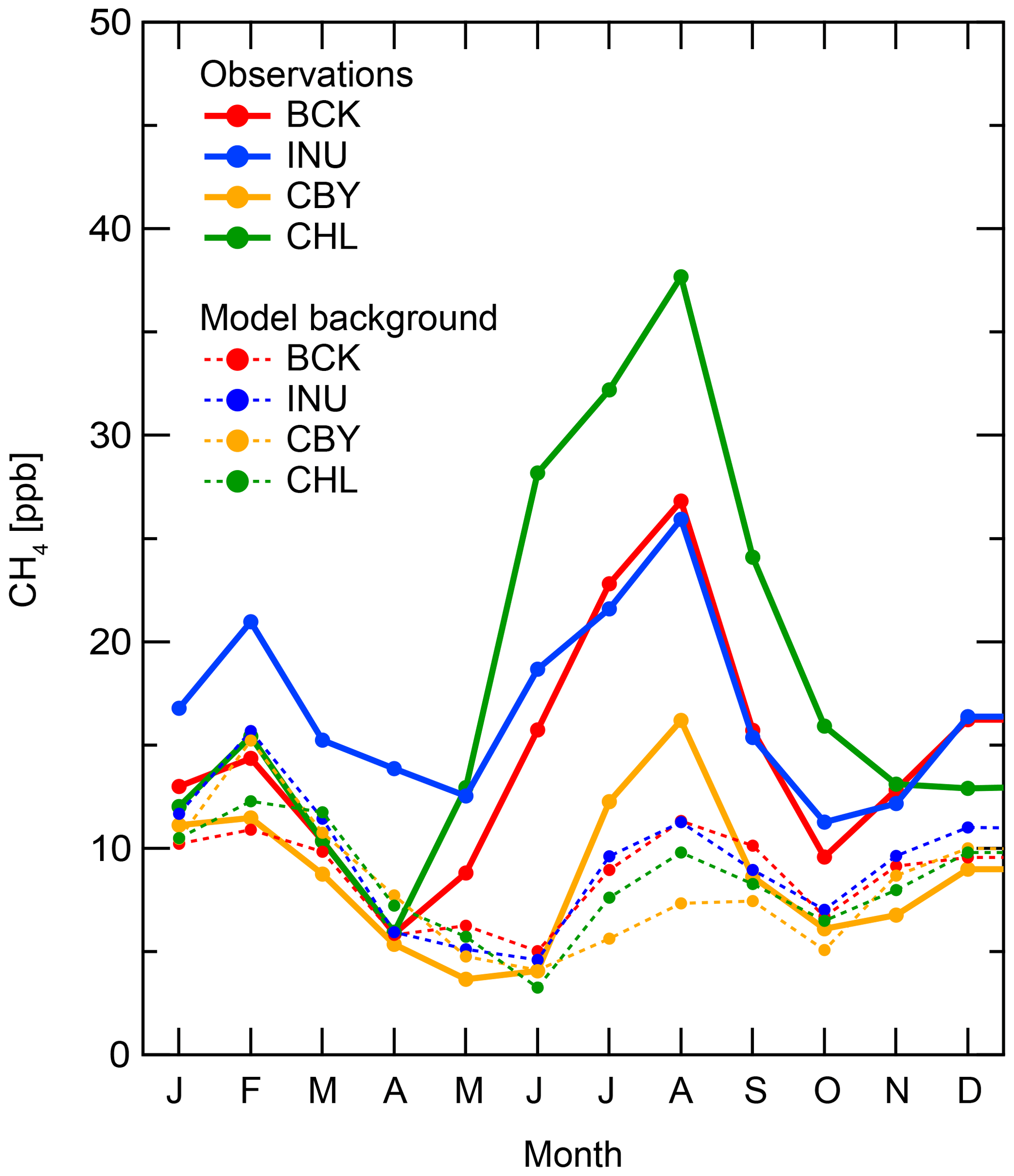
Figure 7The 4-year (2012–2015) mean monthly SD of modelled background CH4 mixing ratios and SD of observed CH4 mixing ratios (afternoon data only, SD_PM). The background CH4 mixing ratios are NIES TM modelled mixing ratios weighted by the endpoints of the 5-day back trajectory.
4.3 Comparison of prior and posterior fluxes with different transport models
The inversion experiments outlined in Table 3 were made to estimate the CH4 fluxes in the Canadian Arctic using atmospheric observations from the four ECCC sites as mentioned in Sect. 3.3.3. We calculated the posterior flux estimates as the mean of the fluxes estimated in the nine experiments in Table 3 (for each set of subregion masks). The variations in the flux results (standard deviation) are used to represent the flux uncertainty due to transport errors (three transport models) and prior flux errors (three prior emission cases). This flux uncertainty is larger than the posterior flux covariance uncertainty estimates, Eq. (3). Figure 8 shows the monthly posterior fluxes with subregion masks A and B. The monthly posterior fluxes with mask C are shown in Fig. S5, along with the aggregated fluxes with masks A and B for the entire Canadian Arctic. As shown in Fig. 8a, the fluxes in NT are dominant, and all the posterior fluxes in NT show a clear seasonal cycle and inter-annual variations that are reflected in the total fluxes for the entire Canadian Arctic (Fig. S5). In contrast, no clear seasonal pattern is found for NU and YT (Fig. 8a and b). The inversion model has difficulty optimizing the weak flux regions. As a result, negative mean fluxes, i.e., CH4 sinks, could appear, especially in YT (Fig. 8a); the negative biomass burning fluxes are “spurious” since the biomass burning CH4 source cannot be negative. However, a null flux would be consistent within error bars.
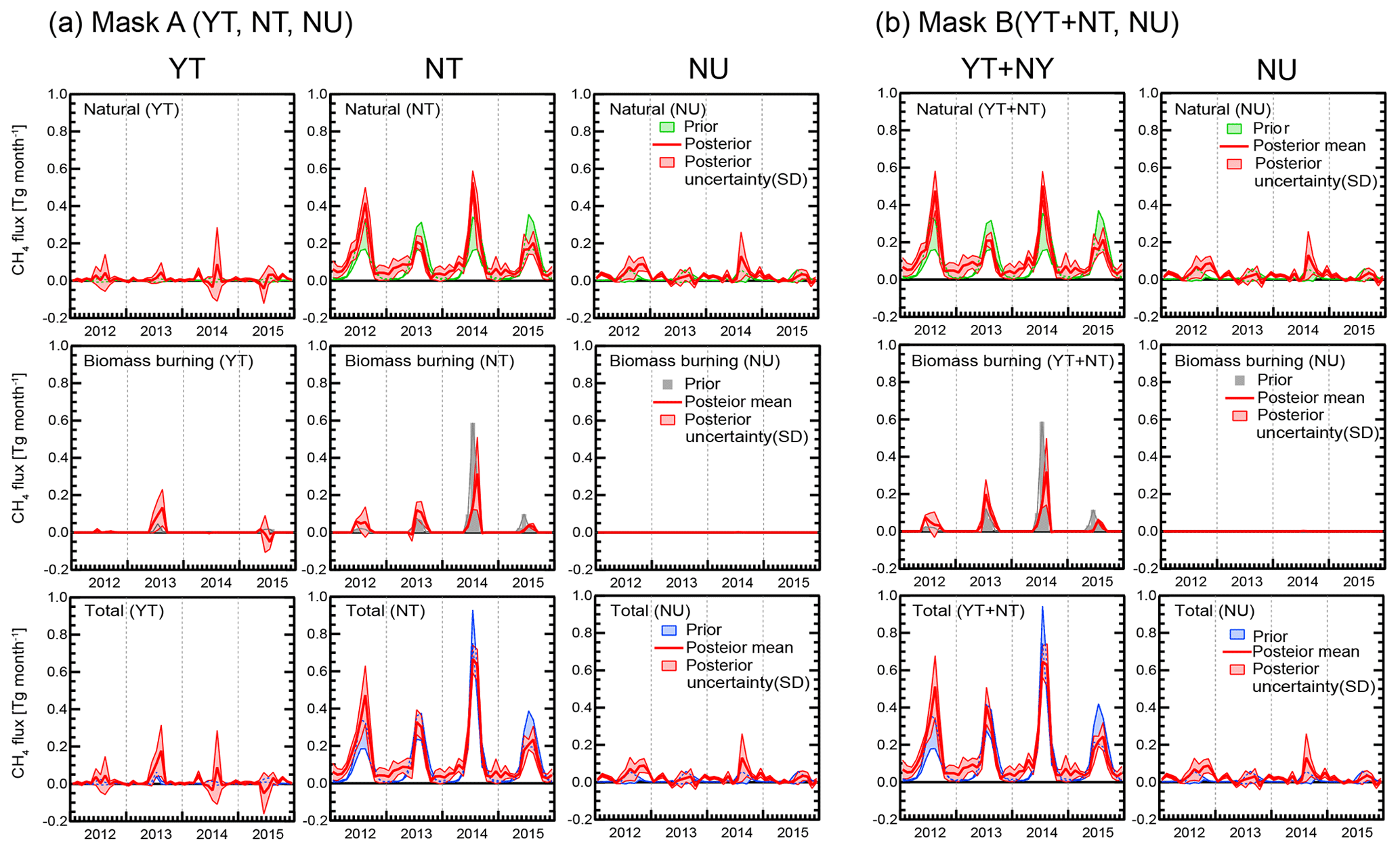
Figure 8Monthly posterior mean fluxes with (a) subregion mask A (YT, NT, NU) and (b) mask B (YT + NT, NU). Posterior mean flux is an average of nine experiments with three models (FLEXPART_EI, FLEXPART_JRA55, and WRF-STILT) and three prior emission cases (VIS, GEL, and WetC). The posterior SD is shown by the red shaded area. Prior fluxes for natural emissions include wetland flux, soil uptake, and anthropogenic emissions. Biomass burning prior fluxes are from GFAS. The (non-red) shaded areas for natural and total prior fluxes indicate the range of prior fluxes.
Next, the differences and similarities in the inversion results from the three transport models are summarized. The differences in the flux estimates by the three different transport models can be seen in Fig. 9. Figure 9 displays the results for YT + NT with mask B by the three different transport models. FLEXPART_JRA55 tends to estimate higher total fluxes than the other models, resulting in higher emissions by ∼0.6 Tg CH4 yr−1 than the average of ∼1.8 Tg CH4 yr−1. WRF-STILT tends to yield the lowest estimate among the three models, lower by ∼0.5 Tg CH4 yr−1 than the average. The posterior total fluxes by FLEXPART_EI appear to be moderate. In winter, the FLEXPART-EI fluxes are close to zero, the same with WRF-STILT. These results are consistent with their footprints (mean emission sensitivities) in Fig. 6. Higher footprint sensitivities near the sites tend to yield lower posterior fluxes and vice versa.

Figure 9Examples of monthly posterior fluxes by nine inversion experiments of three different models (FLEXPART_EI, FLEXPART_JRA55, and WRF-STILT) with three prior emission cases (VIS, GEL, and WetC). The posterior fluxes are plotted for subregion YT + NT in mask B. The posterior flux means of nine experiments with mask B are also plotted. These monthly fluxes are for the year 2014.
The inter-model differences in the posterior forest fire fluxes (biomass burning, BB) are quite noticeable in 2014, which is the extreme fire year in NT. Due to the sporadic nature of the fire events, the differences in transport (transport errors) are evident in the modelled prior CH4 mixing ratios (Fig. S6c) and could lead to substantial differences in the posterior fluxes (Fig. 9). The WRF-STILT estimated BB in 2014 appears to be moderate (0.23 Tg CH4 yr−1), similar to in 2013 (∼0.3 Tg CH4 yr−1), while the other two models show the highest BB flux estimates (0.55–0.67 Tg CH4 yr−1) in 2014, comparable to the prior flux GFAS estimates.
In contrast, the inter-annual variability in total posterior fluxes is very similar among all three transport model results (as shown in Figs. 8 and S5). The inter-annual variability in the transport models (an intra-model result) appears to be consistent, yielding similar posterior flux inter-annual variability. Since all three different transport models capture this inter-annual variability, it appears to be a robust feature of the CH4 source–sink in the Canadian Arctic.
Another robust feature appears to be the similarity in the results for the total Arctic emission with different numbers of subregions used in the inversion. The subregion with strong signals in the prior fluxes (NT) and strong observational constraints (BCK and INU within NT) yielded posterior flux results with small uncertainties, while subregions with weak signals in the prior fluxes (YT) and weak observational constraint (no observations in YT) yielded large uncertainties in the posterior flux estimates. A weak subregion like YT could be combined with another subregion (NT) without a strong impact on the inversion results. The temporal variations in the inversion results with different numbers of subregions (an intra-model result) seem to also be a robust feature. Given that the strong observational constraints and the strong wetland emissions are both located in the central part of the Canadian Arctic, representing the Canadian Arctic as a single region was able to yield reasonable inversion results.
4.4 Comparison with previous estimates
The estimated fluxes for the entire Canadian Arctic in this study are relatively robust in amplitude and temporal variations even with the different prior fluxes and subregion masking. The mean estimated total CH4 annual flux for the Canadian Arctic is 1.8±0.6 Tg CH4 yr−1. Compared with two previous inversion estimates, our estimate is slightly lower than the mean total flux of 2.14 Tg CH4 yr−1 (average from 2009 to 2013) inferred by FLEXINVERT regional inversion (Thompson et al., 2017) but much higher than the estimate of 0.5 Tg CH4 yr−1 (average from 2006 to 2010) from the CarbonTracker-CH4 global inversion (Bruhwiler et al., 2014) (Fig. 10a).
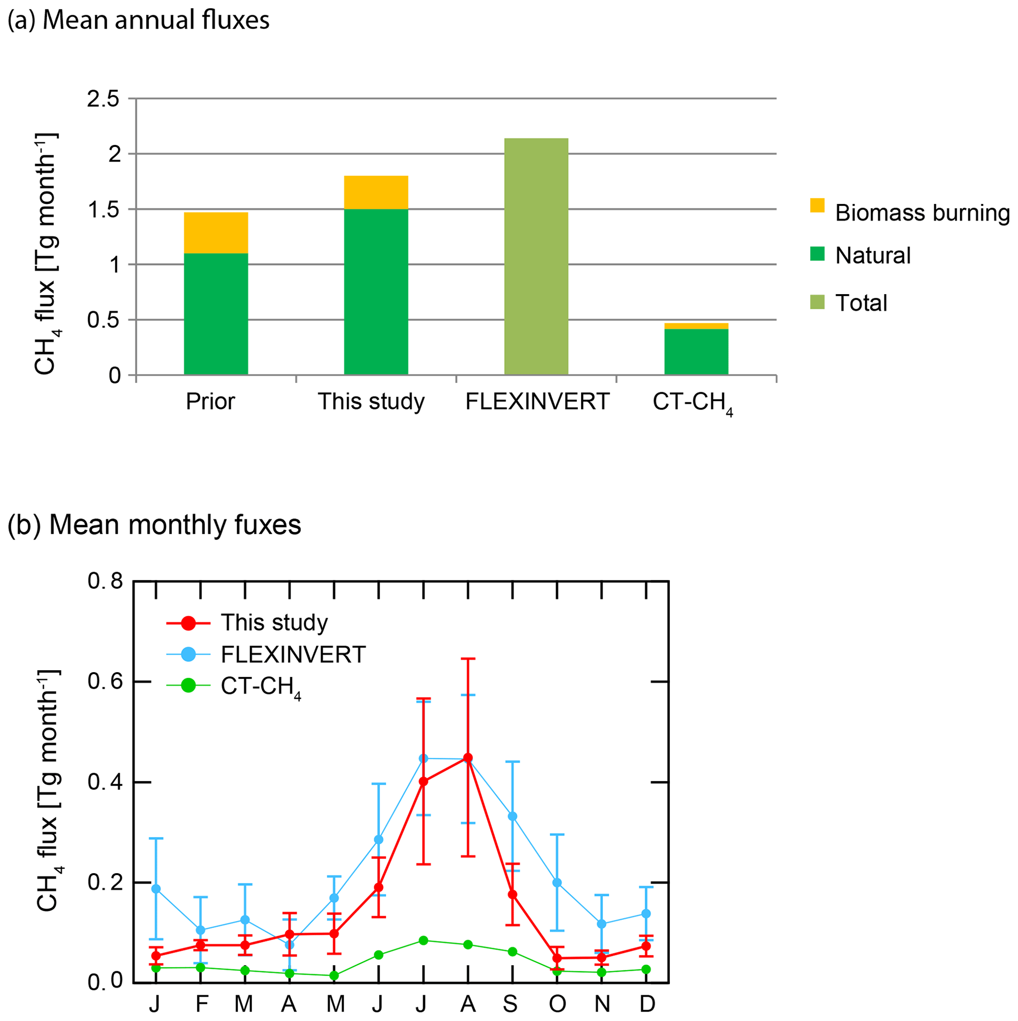
Figure 10Mean prior and posterior (a) annual and (b) monthly fluxes for the Canadian Arctic. FLEXINVERT (Thompson et al., 2017) and CarbonTracker-CH4 (CT-CH4) (Bruhwiler et al., 2014) are plotted for comparison. FLEXINVERT and CT-CH4 fluxes are their last 5-year means, that is, 2009–2013 and 2006–2010 respectively. “Natural” in CT-CH4 is combined with the fluxes estimated as “anthropogenic” and “agriculture”. The bars in monthly fluxes are the SD of multi-year mean monthly fluxes.
All the estimated fluxes are seasonally high around July and August (Fig. 10b). The mean summertime maximum of our estimates is quite consistent with the one by Thompson et al. (2017), but our estimated fluxes have a narrow high summer emission period and low wintertime emission compared with the estimates by Thompson et al. (2017). These temporal differences in estimated fluxes might reflect the observational constraints used in the respective inversions. Thompson et al. (2017) employed a similar type of regional inversion but for the entire northern high latitudes (north of 50∘ N). Except for the flask measurement data at CHL, none of the Canadian Arctic sites used in this study were included in Thompson et al. (2017). The strong regional CH4 signals at INU and BCK in this study appear to yield flux estimates with a narrower high summer emission period and lower wintertime wetland emission compared with the estimates by Thompson et al. (2017).
The flux estimate in this study is partitioned into biomass burning (BB), 0.3±0.1 Tg CH4 yr−1, and the remaining flux, 1.5±0.5 Tg CH4 yr−1. The remaining flux is mainly natural/wetland CH4 emissions, given that anthropogenic contribution to the total prior fluxes without BB is ∼2 % according to the EDGAR prior fluxes. The estimated wetland flux is comparable to the WetCHARTs (wetland) ensemble mean of 1.35 Tg CH4 yr−1 (Bloom et al. 2017a, b).
The estimated summertime natural CH4 fluxes show clear inter-annual variability. The higher emissions are estimated for 2012 and 2014 in this study, which is similar to the results from Carbon Arctic Reservoirs Vulnerability Experiment (CARVE) aircraft measurements over Alaska for 2012 to 2014 (Hartery at al., 2018).
4.5 Relationship of fluxes with climate anomalies
Inter-annual variations in estimated CH4 fluxes are examined in relation to climate parameters, specifically with surface air temperature and precipitation from NCEP reanalysis (Kalnay et al., 1996). First, monthly mean values at the subregions as well as the 4-year mean (2012–2015) for each month are calculated; then the monthly anomalies are computed from the monthly mean values and the 4-year mean of the corresponding month. The temperature and precipitation anomalies are aggregated to the respective regions, NT, YT, and NU. On the regional level, climate anomalies in NT and NU are quite similar, though YT is less similar to NT and NU. YT is mainly covered by mountains with little wetland. Furthermore, among the three Arctic territories, NT has the largest wetland extent and most of the forest fire emissions in 2012–2015. Thus, we look into the correlation in monthly anomalies of CH4 fluxes with summer climate anomalies in NT.
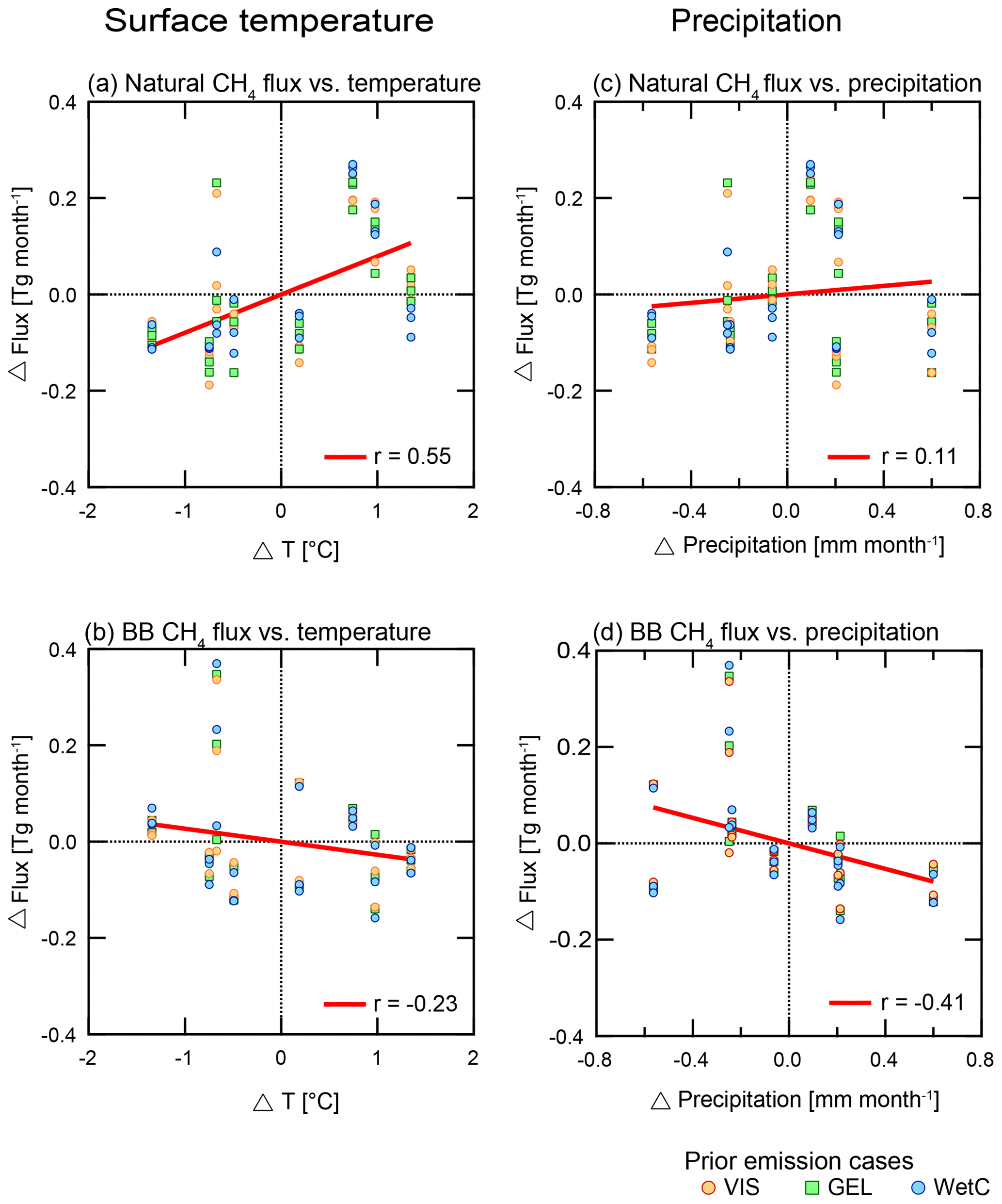
Figure 11CH4 flux anomalies vs. surface temperature and precipitation anomalies for summer (July and August). The CH4 fluxes are July and August posterior fluxes for Northwest Territories (NT) from nine inversion experiments with mask A. Regional climate parameter anomalies in NT are monthly deviations from the 4-year (2012–2015) means.
In Fig. 11, the inter-annual variability of wetland CH4 fluxes exhibits a moderate positive correlation with the surface temperature anomaly (r=0.55) and only weakly correlated with precipitation anomalies (r=0.11). This indicates that the hotter summer weather condition stimulates the wetland CH4 emission, and precipitation appears to have a less immediate or no direct impact on wetland conditions. In prior cases, VIS and GEL, natural CH4 fluxes (wetland and other fluxes except biomass burning CH4 flux) are multi-year mean monthly fluxes. Therefore, these prior fluxes have no year-to-year anomalies and no correlation with the meteorological anomalies. Only in WetC, the prior with wetland CH4 fluxes from WetCHARTs ensemble mean has inter-annual variations, and the correlations with temperature and precipitation anomalies are r=0.26 and r=0.90 respectively. The posterior natural fluxes with WetC show slightly higher correlations (r=0.55 with temperature, r=0.16 with precipitation) than the mean correlation values. However, overall there is no clear dependency of posterior correlations on the inherent climate anomaly correlations in the prior fluxes. This result indicates that the inter-annual variations in posterior wetland fluxes in this study are mainly determined by the observations, rather than by prior fluxes.
Inter-annual variations in estimated BB CH4 fluxes show a negative correlation with precipitation (). Also throughout the fire season (June–September), all estimated BB fluxes negatively correlate with precipitation while the prior BB fluxes appear to have no consistent correlations. The inversion results support that dry conditions would enhance the forest fire. The estimated BB fluxes show a weakly negative correlation with surface temperature () on midsummer average, but the monthly correlations fluctuate from to r=0.47 over the fire season. Since the period is limited in this study (2012–2015), these statistical relationships are still not clear. Also, the relationship of CH4 emissions with climate conditions could be complex and non-linear (with extreme fire events in some years). More data and analysis are required to characterize the dependency of CH4 fluxes on climate in the Arctic.
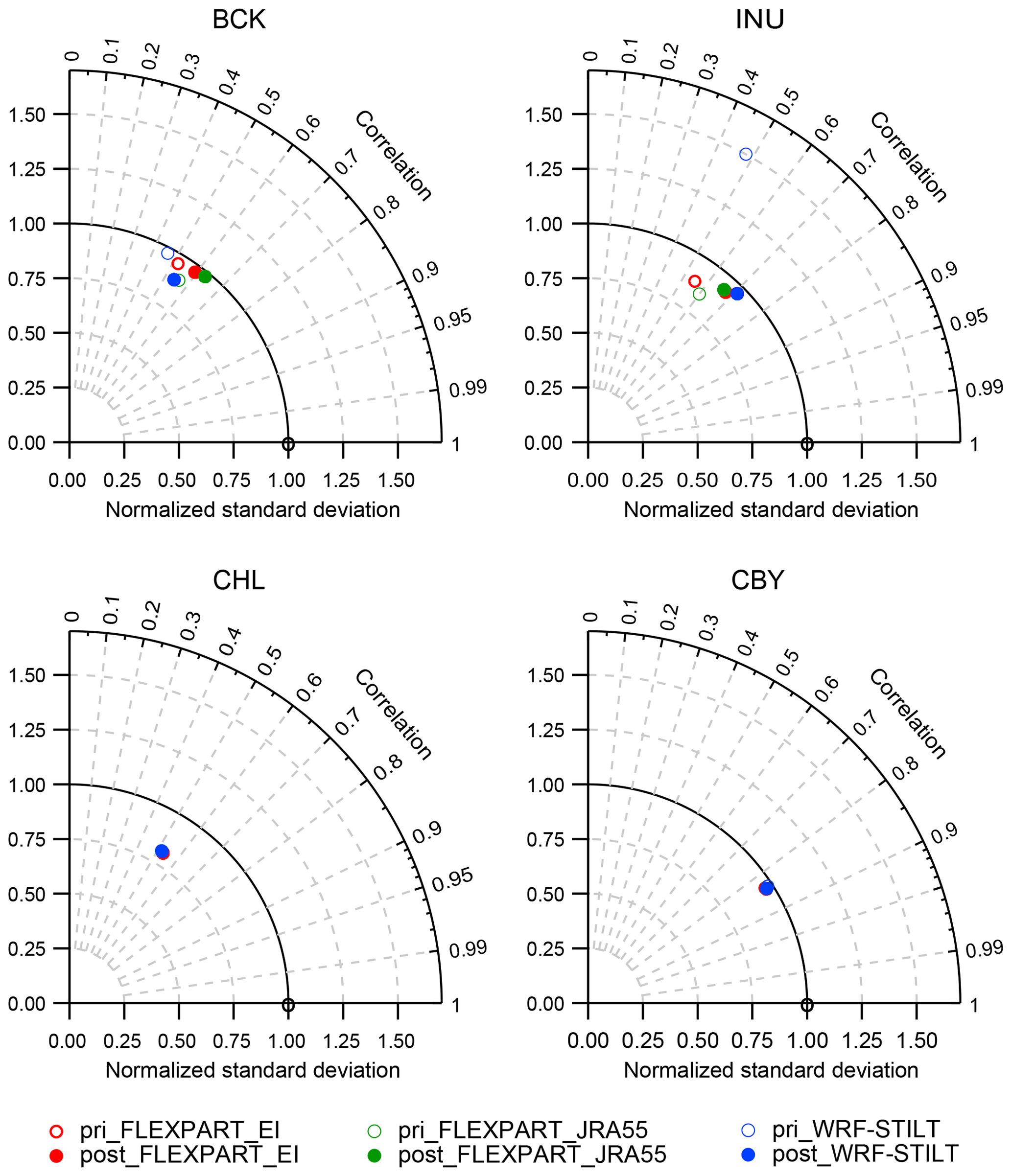
Figure 12Taylor diagrams for the comparison between the prior (open circles) and posterior (closed circles) mixing ratios by three models: FLEXPART_EI (red), FLEXPART_JRA55 (green), and WRF-STILT (blue), with mask B and prior flux case WetC. The radius is the normalized standard deviation (NSD) of modelled mixing ratios against observations. The angle is the correlation coefficient. The values are the means with all observations and modelled mixing ratios for each site.
4.6 Comparison of modelled and observed mixing ratios
The model–observation statistical comparison is shown with the Taylor diagrams of correlation coefficients and normalized standard deviation (NSD) by three different transport models for the four Arctic sites (Fig. 12) using the inversion results with mask B and prior flux case WetC. At BCK and INU, the correlation coefficients and NSD for each model are improved by the inversion. At these two sites, the observations contain large synoptic signals from the Canadian Arctic wetland and provide strong constraints to the inversions. At INU, the improvement for STILT is noticeable, especially with NSD. This improvement of STILT is explained further below. At CBY and CHL, no significant changes between the prior and posterior results are seen. This indicates that the regional flux in the Canadian Arctic only weakly influences CBY and CHL.
Further investigation has been conducted for INU. Figure S7a shows the time series of modelled prior and posterior mixing ratios by the three transport models and the observed mixing ratio. The Taylor diagrams in Fig. S7b show the comparison results of modelled mixing ratios with the observations by season, summer months (June–September) and winter months (October-May), as well as for the entire period together. The modelled mixing ratios by STILT with the prior fluxes could be much higher than the mixing ratios by the other two models. That results in the higher prior NSD values, especially in the winter season. The inversion was able to improve the results by reducing the fluxes and consequently the posterior NSD.
Another qualitative measure of the goodness of fit of the model to the observations is the reduced chi-square statistics (Drosg, 2009; Hughes and Hase, 2010). For the limiting case of an infinite number of data points, the data are independent and normally distributed, and the value of reduced chi-square should be 1. The overall reduced chi-squares for all our experiments are in a narrow range of 1.23–1.27. Given that the observations and modelled mixing ratios are not normally distributed (more frequent high mixing ratio events than low mixing ratio events) and the limited number of observations, there does not seem to be a strong reason to reject the model results.
4.7 Sensitivity tests
4.7.1 Prior fluxes: wetland CH4 fluxes
Wetland CH4 emissions are the dominant flux in the Canadian Arctic. To examine how the prior fluxes impact the posterior fluxes, two inversion experiments were conducted with modified WetCHARTs fluxes. One is 50 % reduced emissions in the Canadian Arctic and another is 50 % increased emissions in the Canadian Arctic. The results are shown as mean posterior natural fluxes in Fig. S8. Despite the change in wetland prior emissions, all the posterior fluxes are similar to the ones in the control case; the changes in the posterior fluxes are less than 5 % annually. This indicates that the posterior fluxes are not very sensitive to the amplitude/strength of prior fluxes.
4.7.2 Contributions of background CH4 mixing ratios on the posterior fluxes
We used the same background CH4 mixing ratios for the different transport models, which are calculated using the particle endpoints from FLEXPART_JRA55. The idea of using the same background CH4 fields is to focus on the impact of the local and regional transport contribution on regional inversion, separating from the background contribution.
One notable feature in the background CH4 mixing ratios is the relatively large synoptic variability, especially in winter compared to the observed CH4, which might contribute to large uncertainties in flux estimation. To examine how sensitive the inversion results are to these temporal variations in the background CH4 mixing ratios, additional experiments with background CH4 with smoothing windows of 5 days, 10 days, and 30 days were made (see Fig. S9a).
The examples of the results are shown in Fig. S9b and c. The posterior fluxes are not strongly dependent on the different background CH4 mixing ratios. Compared with the unsmoothed background case, slightly small values of NSD are found in the model–observation statistical comparison for summer with 30-day smoothing. It seems there are sufficient observations (signal level) above the background CH4 mixing ratios (noise level) to constrain the inversion results (Fig. 7).
The Canadian Arctic region is one of the potential enhanced CH4 source regions related to the ongoing global warming (AMAP, 2015). Earth system models differ in their prediction of how the carbon loss in this region will be split up between CO2 and CH4 emissions. Even current bottom-up and top-down estimates of CH4 flux in the region vary widely. This study
-
analyzed the measurements of atmospheric CH4 mixing ratios from five sites established in the Canadian Arctic by ECCC to characterize the observed variations and examine the detectability of regional fluxes,
-
estimated the regional fluxes for 4 years (2012–2015) with the continuous observational data of atmospheric CH4 and also examined the relationship of the estimated fluxes with the climate anomalies.
The observational data analysis reveals large synoptic summertime signals in the atmospheric CH4, indicating strong regional fluxes (most likely wetland and biomass burning CH4 emissions) around Behchoko and Inuvik in Northwest Territory, the western Canadian Arctic. The local signals of atmospheric CH4 also allow inverse models to optimize biomass burning CH4 flux (emissions due to forest fire), separately from the natural CH4 fluxes.
The estimated mean total CH4 annual flux for the Canadian Arctic is 1.8±0.6 Tg CH4 yr−1 (wetland flux is 1.5±0.5 Tg CH4 yr−1, biomass burning flux 0.3±0.1 Tg CH4 yr−1). The mean total flux in this study is comparable to another regional flux inversion result of 2.14 Tg CH4 yr−1 by Thompson et al. (2017) but much higher than the global inversion result of 0.5 Tg CH4 yr−1 by CarbonTracker-CH4 (Bruhwiler et al., 2014). The strong regional CH4 signals at INU and BCK appear to yield flux estimates in this study with a narrower high summer emission period and lower wintertime wetland emission compared with the estimates by Thompson et al. (2017).
Clear inter-annual variability is found in all the estimated summertime natural CH4 fluxes for the Canadian Arctic, mostly due to Northwest Territories. These summertime flux variations are positively correlated with the surface temperature anomaly (r=0.55). This result indicates that years with warmer summer conditions result in more wetland CH4 emissions.
With longer data records and more analysis in the Arctic, inversion CH4 flux estimates could yield more details on CH4 emission strength and seasonal cycle (onset and termination of wetland emissions) and dependence of wetland fluxes on climate conditions. More knowledge on the flux and climate relationship could help evaluate and improve bottom-up wetland CH4 flux models.
Next, we will perform a similar study for the CO2 measurements from these sites to estimate the Canadian Arctic CO2 fluxes. Estimation of CO2 and CH4 fluxes and monitoring how these fluxes change in the future will improve our understanding of the response of the Arctic carbon cycle to climate change and also yield long-term trends in CO2 and CH4 emissions in the Canadian Arctic.
The data measured at ECCC sites used in this study are available upon request to Doug Worthy (doug.worthy@canada.ca). The Alert data are also periodically updated to WDCGG, http://ds.data.jma.go.jp/gmd/wdcgg (WDCGG, 2019). The model-related data are available upon request to the corresponding author.
The supplement related to this article is available online at: https://doi.org/10.5194/acp-19-4637-2019-supplement.
MI and DC designed the research and prepared the paper. MI performed data analysis and inversion experiments. DW led the measurement programs and collected the observational data. MI, DC, and EC provided footprint (potential emission sensitivities) information for inversions. All authors contributed to the discussion and interpretation of the results.
The authors declare that they have no conflict of interest.
We acknowledge the CarbonTracker Lagrange (CT-L) program for providing the WRF-STILT footprint data for our inversion study. CT Lagrange has been supported by the NOAA Climate Program Office's Atmospheric Chemistry, Carbon Cycle, and Climate (AC4) Program and the NASA Carbon Monitoring System. We would like to extend our gratitude to the conscientious care taken by the program technicians, Robert Kessler and Larry Giroux, and IT support provided by Senen Racki. Appreciation is also forwarded to the Northwest Territories Power Corporation (NTPC) for making available their building facility to house our equipment and tower to string our sampling lines. NTPC also provided IT communication to permit access to our equipment and transmission of data. We thank Lori Bruhwiler for the use of CT-CH4 data, Rona Thompson for providing FLEXINVERT CH4 fluxes, and Peter Bergamaschi for providing TM5-4DVAR inversion results.
This paper was edited by Mathias Palm and reviewed by two anonymous referees.
AMAP: Assesment 2015: Methane as an Arctic clilmate forcer, Arctic Monitoring ans Assessment Programme (AMAP), Oslo, Norway, 2015.
Belikov, D. A., Maksyutov, S., Sherlock, V., Aoki, S., Deutscher, N. M., Dohe, S., Griffith, D., Kyro, E., Morino, I., Nakazawa, T., Notholt, J., Rettinger, M., Schneider, M., Sussmann, R., Toon, G. C., Wennberg, P. O., and Wunch, D.: Simulations of column-averaged CO2 and CH4 using the NIES TM with a hybrid sigma-isentropic (σ-θ) vertical coordinate, Atmos. Chem. Phys., 13, 1713–1732, https://doi.org/10.5194/acp-13-1713-2013, 2013.
Bergamaschi, P., Houweling, S., Segers, A., Krol, M., Frankenberg, C., Scheepmaker, R. A., Dlugokencky, E., Wofsy, S. C., Kort, E. A., Sweeney, C., Schuck, T., Brenninkmeijer, C., Chen, H., Beck, V., and Gerbig, C.: Atmospheric CH4 in the first decade of the 21st century: Inverse modeling analysis using SCIAMACHY satellite retrievals and NOAA surface measurements, J. Geophys. Res., 118, 7350–7369, https://doi.org/10.1002/jgrd.50480, 2013.
Bloom, A. A., Bowman, K. W., Lee, M., Turner, A. J., Schreder, R., Worden, J. R., Wedner, R. J., Mcdonald, K. C., and Jacob, D. J.: CMS: Global 0.5-deg Wetland Methane Emissions and Uncertainty (WetCHARTs v1.0), ORNL Distributed Active Archive Center, https://doi.org/10.3334/ORNLDAAC/1502, 2017a.
Bloom, A. A., Bowman, K. W., Lee, M., Turner, A. J., Schroeder, R., Worden, J. R., Weidner, R., McDonald, K. C., and Jacob, D. J.: A global wetland methane emissions and uncertainty dataset for atmospheric chemical transport models (WetCHARTs version 1.0), Geosci. Model Dev., 10, 2141–2156, https://doi.org/10.5194/gmd-10-2141-2017, 2017b.
Bousquet, P., Ringeval, B., Pison, I., Dlugokencky, E. J., Brunke, E. G., Carouge, C., Chevallier, F., Fortems-Cheiney, A., Frankenberg, C., Hauglustaine, D. A., Krummel, P. B., Langenfelds, R. L., Ramonet, M., Schmidt, M., Steele, L. P., Szopa, S., Yver, C., Viovy, N., and Ciais, P.: Source attribution of the changes in atmospheric methane for 2006–2008, Atmos. Chem. Phys., 11, 3689–3700, https://doi.org/10.5194/acp-11-3689-2011, 2011.
Bruhwiler, L., Dlugokencky, E., Masarie, K., Ishizawa, M., Andrews, A., Miller, J., Sweeney, C., Tans, P., and Worthy, D.: CarbonTracker-CH4: an assimilation system for estimating emissions of atmospheric methane, Atmos. Chem. Phys., 14, 8269–8293, https://doi.org/10.5194/acp-14-8269-2014, 2014.
CarbonTracker-Lagrange: National Oceanic & Atmospheric Administration, Earth System Research Laboratory (NOAA/ESRL), available at: https://www.esrl.noaa.gov/gmd/ccgg/carbontracker-lagrange/, last access: 1 February 2019.
Chan, D., Yuen C. W., Higuchi, K., Shashkov, A., Liu, J., Chen, J., and Worthy, D.: On the CO2 exchange between the atmosphere and the biosphere: the role of synoptic and mesoscale processes, Tellus B, 56, 194–212, 2004.
Chang, R. Y.-W., Miller, C. E., Dinardo, S. J., Karion, A., Sweeney, C., Daube, B. C., Henderson, J. M., Mountain, M. E., Eluszkiewicz, J., Miller, J. B., Bruhwiler, L. M. P., and Wofsy, S. C.: Methane emissions from Alaska in 2012 from CARVE airborne observations, P. Natl. Acad. Sci. USA, 111, 16694–16699, https://doi.org/10.1073/pnas.1412953111, 2014
Ciais, P., Sabine, C., Bala, G., Bopp, L., Brovkin, V., Canadell, J., Chhabra, A., DeFries, R., Galloway, J., Heimann, M., Jones, C., Le Queìreì, C., Myneni, R. B., Piao, S., and Thornton, P.: Carbon and Other Biogeochemical Cycles, in: Climate Change 2013: The Physical Science Basis. Contribution of Working Group I to the Fifth Assessment Report of the Intergovernmental Panel on Climate Change, edited by: Stocker, T. F., Qin, D., Plattner, G.-K., Tignor, M., Allen, S. K., Boschung, J., Nauels, A., Xia, Y., Bex, V., and Midgley, P. M., Cambridge University Press, Cambridge, United Kingdom and New York, NY, USA, 465–570, 2013.
Cooper, O. R., Parrish, D. D., Stohl, A., Trainer, M., Nédélec, P., Thouret, V., Cammas, J. P., Oltmans, S. J., Johnson, B. J., Tarasick, D., Leblanc, T., McDermid, I. S., Jaffe, D., Gao, R., Stith, J., Ryerson, T., Aikin, K., Campos, T., Weinheimer, A., and Avery, M. A.: Increasing springtime ozone mixing ratios in the free troposphere over western North America, Nature, 463, 344–348, https://doi.org/10.1038/nature08708
Dee, D. P., Uppala, S. M., Simmons, A. J., Berrisford, P., Poli, P., Kobayashi, S., Andrae, U., Balmaseda, M. A., Balsamo, G., Bauer, P., Bechtold, P., Beljaars, A. C. M., van de Berg, L., Bidlot, J., Bormann, N., Delsol, C., Dragani, R., Fuentes, M., Geer, A. J., Haimberger, L., Healy, S. B., Hersbach, H., Hólm, E. V., Isaksen, L., Kållberg, P., Köhler, M., Matricardi, M., McNally, A. P., Monge-Sanz, B. M., Morcrette, J. J., Park, B. K., Peubey, C., de Rosnay, P., Tavolato, C., Thépaut, J. N., and Vitart, F.: The ERA-Interim reanalysis: configuration and performance of the data assimilation system, Q. J. R. Meteorol. Soc., 137, 553–597, https://doi.org/10.1002/qj.828, 2011.
Dlugokencky, E. J.: Trends in Atmospheric Methane, National Oceanic & Atmospheric Administration, Earth System Research Laboratory (NOAA/ESRL), available at: http://www.esrl.noaa.gov/gmd/ccgg/trends_ch4/, last access: 1 August 2018.
Dlugokencky, E. J., Myers, R. C., Lang, P. M., Masarie, K. A., Crotwell, A. M., Thoning, K. W., Hall, B. D., Elkins, J. W., and Steele, L. P.: Conversion of NOAA atmospheric dry air CH4 mole fractions to a gravimetrically prepared standard scale, J. Geophys. Res., 110, D18306, https://doi.org/10.1029/2005JD006035, 2005.
Drosg, M.: Dealing with Uncertainties: A Guide to Error Analysis, Springer-Verlag Berlin Heidelberg, Dordrecht, 252 pp., 2009.
EDGARv4.2FT2010: European Commission, Joint Research Centre (JRC)/Netherlands Environmental Assessment Agency (PBL), Emission Database for Global Atmospheric Research (EDGAR), release EDGARv4.2FT2010, available at: http://edgar.jrc.ec.europa.eu, last access: 1 August 2018, 2014.
Enting, I. G.: Inverse Problems in Atmospheric Constituent Transport, Cambridge University Press, Cambridge, UK, 392 pp., 2002.
Fung, I., John, J., Lerner, J., Matthews, E., Prather, M., Steele, L. P., and Fraser, P. J.: Three-dimensional model synthesis of the global methane cycle, J. Geophys. Res., 96, 13033–13065, https://doi.org/10.1029/91JD01247, 1991.
Gasser, T., Peters, G. P., Fuglestvedt, J. S., Collins, W. J., Shindell, D. T., and Ciais, P.: Accounting for the climate–carbon feedback in emission metrics, Earth Syst. Dynam., 8, 235–253, https://doi.org/10.5194/esd-8-235-2017, 2017.
Gerbig, C., Lin, J. C., Wofsy, S. C., Daube, B. C., Andrews, A. E., Stephens, B. B., Bakwin, P. S., and Grainger, C. A.: Toward constraining regional-scale fluxes of CO2 with atmospheric observations over a continent: 2. Analysis of COBRA data using a receptor-oriented framework, J. Geophys. Res., 108, 4757, https://doi.org/10.1029/2003JD003770, 2003.
Gloor, M., Bakwin, P., Hurst, D., Lock, L., Draxler, R., and Tans, P.: What is the concentration footprint of a tall tower?, J. Geophys. Res., 106, 17831–17840, https://doi.org/10.1029/2001JD900021, 2001.
Harada, Y., Kamahori, H., Kobayashi, C., Endo, H., Kobayashi, S., Ota, Y., Onoda, H., Onogi, K., Miyaoka, K., and Takahashi, K.: The JRA-55 Reanalysis: Representation of Atmospheric Circulation and Climate Variability, J. Meteor. Soc. Jpn., 94, 269–302, https://doi.org/10.2151/jmsj.2016-015, 2016.
Hartery, S., Commane, R., Lindaas, J., Sweeney, C., Henderson, J., Mountain, M., Steiner, N., McDonald, K., Dinardo, S. J., Miller, C. E., Wofsy, S. C., and Chang, R. Y.-W.: Estimating regional-scale methane flux and budgets using CARVE aircraft measurements over Alaska, Atmos. Chem. Phys., 18, 185–202, https://doi.org/10.5194/acp-18-185-2018.
Henderson, J. M., Eluszkiewicz, J., Mountain, M. E., Nehrkorn, T., Chang, R. Y. W., Karion, A., Miller, J. B., Sweeney, C., Steiner, N., Wofsy, S. C., and Miller, C. E.: Atmospheric transport simulations in support of the Carbon in Arctic Reservoirs Vulnerability Experiment (CARVE), Atmos. Chem. Phys., 15, 4093–4116, https://doi.org/10.5194/acp-15-4093-2015, 2015.
Hu, L., Andrews, A. E., Thoning, K. W., Sweeney, C., Miller, J. B., Michalak, A. M., Dlugokencky, E., Tans, P. P., Shiga, Y. P., Mountain, M., Nehrkorn, T., Montzka, S. A., McKain, K., Kofler, J., Trudeau, M., Michel, S. E., Biraud, S. C., Fischer, M. L., Worthy, D. E. J, Vaughn, B., White, J. W. C., Yadav, V., Basu, S., and van der Velde I. R.: Enhanced North American carbon uptake associated with El Nino, Sci. Adv., accepted, 2019.
Hughes, I. G. and Hase, T.: Measurements and their Uncertainties: A Practical Guide to Modern Error Analysis, Oxford University Press, New York, 160 pp., 2010.
Ishizawa, M., Mabuchi, K., Shirai, T., Inoue, M., Morino, I., Uchino, O., Yoshida, Y., Belikov, D., and Maksyutov, S.: Inter-annual variability of summertime CO2 exchange in Northern Eurasia inferred from GOSAT XCO2, Environ. Res. Lett., 11, 105001, https://doi.org/10.1088/1748-9326/11/10/105001, 2016.
Ito, A. and Inatomi, M.: Use of a process-based model for assessing the methane budgets of global terrestrial ecosystems and evaluation of uncertainty, Biogeosciences, 9, 759–773, https://doi.org/10.5194/bg-9-759-2012, 2012.
Jammet, M., Crill, P., Dengel, S., and Friborg, T.: Large methane emissions from a subarctic lake during spring thaw: Mechanisms and landscape significance, J. Geophys. Res., 120, 2289–2305, https://doi.org/10.1002/2015JG003137, 2015.
Kaiser, J. W., Heil, A., Andreae, M. O., Benedetti, A., Chubarova, N., Jones, L., Morcrette, J. J., Razinger, M., Schultz, M. G., Suttie, M., and van der Werf, G. R.: Biomass burning emissions estimated with a global fire assimilation system based on observed fire radiative power, Biogeosciences, 9, 527–554, https://doi.org/10.5194/bg-9-527-2012, 2012.
Kalnay, E., Kanamitsu, M., Kistler, R., Collins, W., Deaven, D., Gandin, L., Iredell, M., Saha, S., White, G., Woollen, J., Zhu, Y., Leetmaa, A., Reynolds, R., Chelliah, M., Ebisuzaki, W., Higgins, W., Janowiak, J., Mo, K. C., Ropelewski, C., Wang, J., Roy, J., and Dennis, J.: The NCEP/NCAR 40-Year Reanalysis Project, Bull. Am. Meteorol. Soc., 77, 437–471, 1996.
Karion, A., Sweeney, C., Miller, J. B., Andrews, A. E., Commane, R., Dinardo, S., Henderson, J. M., Lindaas, J., Lin, J. C., Luus, K. A., Newberger, T., Tans, P., Wofsy, S. C., Wolter, S., and Miller, C. E.: Investigating Alaskan methane and carbon dioxide fluxes using measurements from the CARVE tower, Atmos. Chem. Phys., 16, 5383–5398, https://doi.org/10.5194/acp-16-5383-2016, 2016.
Kirschke, S., Bousquet, P., Ciais, P., Saunois, M., Canadell, J. G., Dlugokencky, E. J., Bergamaschi, P., Bergmann, D., Blake, D. R., Bruhwiler, L., Cameron-Smith, P., Castaldi, S., Chevallier, F., Feng, L., Fraser, A., Heimann, M., Hodson, E. L., Houweling, S., Josse, B., Fraser, P. J., Krummel, P. B., Lamarque, J.-F., Langenfelds, R. L., Le Quéré, C., Naik, V., O'Doherty, S., Palmer, P. I., Pison, I., Plummer, D., Poulter, B., Prinn, R. G., Rigby, M., Ringeval, B., Santini, M., Schmidt, M., Shindell, D. T., Simpson, I. J., Spahni, R., Steele, L. P., Strode, S. A., Sudo, K., Szopa, S., van der Werf, G. R., Voulgarakis, A., van Weele, M., Weiss, R. F., Williams, J. E., and Zeng, G.: Three decades of global methane sources and sinks, Nat. Geosci., 6, 813–823, https://doi.org/10.1038/ngeo1955, 2013.
Kobayashi, S., Ota, Y., Harada, Y., Ebita, A., Moriya, M., Onoda, H., Onogi, K., Kamahori, H., Kobayashi, C., Endo, H., Miyaoka, K., and Takahashi, K.: The JRA-55 Reanalysis: General Specifications and Basic Characteristics, J. Meteor. Soc. Jpn., 93, 5–48, https://doi.org/10.2151/jmsj.2015-001, 2015.
Lehner, B. and Döll, P.: Development and validation of a global database of lakes, reservoirs and wetlands, J. Hydrol., 296, 1–22, https://doi.org/10.1016/j.jhydrol.2004.03.028, 2004.
Lin, J. C. and Gerbig, C.: Accounting for the effect of transport errors on tracer inversions, Geophys. Res. Lett., 32, L01802, https://doi.org/10.1029/2004GL021127, 2005.
Lin, J. C., Gerbig, C., Wofsy, S. C., Andrews, A. E., Daube, B. C., Davis, K. J., and Grainger, C. A.: A near-field tool for simulating the upstream influence of atmospheric observations: The Stochastic Time-Inverted Lagrangian Transport (STILT) model, J. Geophys. Res.-Atmos., 108, 4493, https://doi.org/10.1029/2002jd003161, 2003.
Lin, J. C., Gerbig, C., Wofsy, S. C., Andrews, A. E., Daube, B. C., Grainger, C. A., Stephens, B. B., Bakwin, P. S., and Hollinger, D. Y.: Measuring fluxes of trace gases at regional scales by Lagrangian observations: Application to the CO2 Budget and Rectification Airborne (COBRA) study, J. Geophys. Res., 109, D15304, https://doi.org/10.1029/2004JD004754, 2004.
McGuire, A. D., Anderson, L. G., Christensen, T. R., Dallimore, S., Guo, L., Hayes, D. J., Heimann, M., Lorenson, T. D., Macdonald, R. W., and Roulet, N.: Sensitivity of the carbon cycle in the Arctic to climate change, Ecol. Monogr., 79, 523–555, https://doi.org/10.1890/08-2025.1, 2009
Melton, J. R., Wania, R., Hodson, E. L., Poulter, B., Ringeval, B., Spahni, R., Bohn, T., Avis, C. A., Beerling, D. J., Chen, G., Eliseev, A. V., Denisov, S. N., Hopcroft, P. O., Lettenmaier, D. P., Riley, W. J., Singarayer, J. S., Subin, Z. M., Tian, H., Zürcher, S., Brovkin, V., van Bodegom, P. M., Kleinen, T., Yu, Z. C., and Kaplan, J. O.: Present state of global wetland extent and wetland methane modelling: conclusions from a model inter-comparison project (WETCHIMP), Biogeosciences, 10, 753–788, https://doi.org/10.5194/bg-10-753-2013, 2013.
Miller, S. M., Worthy, D. E. J., Michalak, A. M., Wofsy, S. C., Kort, E. A., Havice, T. C., Andrews, A. E., Dlugokencky, E. J., Kaplan, J. O., Levi, P. J., Tian, H., and Zhang, B.: Observational constraints on the distribution, seasonality, and environmental predictors of North American boreal methane emissions, Global Biogeochem. Cy., 28, 146–160, https://doi.org/10.1002/2013GB004580, 2014.
Miller, S. M., Miller, C. E., Commane, R., Chang, R. Y.-W., Dinardo, S. J., Henderson, J. M., Karion, A., Lindaas, J., Melton, J. R., Miller, J. B., Sweeney, C., Wofsy, S. C., and Michalak, A. M.: A multiyear estimate of methane fluxes in Alaska from CARVE atmospheric observations, Global Biogeochem. Cy., 30, 1441–1453, https://doi.org/10.1002/2016GB005419, 2016.
Nakazawa, T., Ishizawa, M., Higuchi, K., and Trivett, N. B. A.: Two curve fitting methods applied to CO2 flask data, Environmtrics, 8, 197–218, 1997.
Olefeldt, D., Goswami, S., Grosse, G., Hayes, D., Hugelius, G., Kuhry, P., McGuire, A. D., Romanovsky, V. E., Sannel, A. B. K., Schuur, E. A. G., and Turetsky, M. R.: Circumpolar distribution and carbon storage of thermokarst landscapes, Nat. Commun., 7, 13043, https://doi.org/10.1038/ncomms13043, 2016.
Patra, P. K., Houweling, S., Krol, M., Bousquet, P., Belikov, D., Bergmann, D., Bian, H., Cameron-Smith, P., Chipperfield, M. P., Corbin, K., Fortems-Cheiney, A., Fraser, A., Gloor, E., Hess, P., Ito, A., Kawa, S. R., Law, R. M., Loh, Z., Maksyutov, S., Meng, L., Palmer, P. I., Prinn, R. G., Rigby, M., Saito, R., and Wilson, C.: TransCom model simulations of CH4 and related species: linking transport, surface flux and chemical loss with CH4 variability in the troposphere and lower stratosphere, Atmos. Chem. Phys., 11, 12813–12837, https://doi.org/10.5194/acp-11-12813-2011, 2011.
Poulter , B., Bousquet, P., Canadell, J., G. , Philippe, C., Philippe, Peregon, A., Marielle, S., Arora, V., K., Beerling, D., J. , Victor, B., Chris, D. J., Fortunat, J., Nicola, G., Akihito, I., Thomas, K., Charles, D. K., Kyle, M., Joe, R. M., Changhui, P., Shushi, P., Catherine, P., Ronny, S., William, J. R., Makoto, S., Renato, S., Hanqin, T., Lyla, T., Nicolas, V., David, W., Andy, W., Xiyan, X., Bowen, Z., Zhen, Z., and Qiuan, Z.: Global wetland contribution to 2000–2012 atmospheric methane growth rate dynamics, Environ. Res. Lett., 12, 094013, https://doi.org/10.1088/1748-9326/aa8391, 2017.
Rodgers, C. D.: Inverse Methods for Atmospheric Sounding: Theory and Practice, World Scientific, Singapore, 240 pp., 2000.
Sasakawa, M., Shimoyama, K., Machida, T., Tsuda, N., Suto, H., Arshinov, M., Davydov, D., Fofonov, A., Krasnov, O., Saeki, T., Koyama, Y., and Maksyutov, S.: Continuous measurements of methane from a tower network over Siberia, Tellus B, 62, 403–416, https://doi.org/10.1111/j.1600-0889.2010.00494.x, 2010.
Saunois, M., Bousquet, P., Poulter, B., Peregon, A., Ciais, P., Canadell, J. G., Dlugokencky, E. J., Etiope, G., Bastviken, D., Houweling, S., Janssens-Maenhout, G., Tubiello, F. N., Castaldi, S., Jackson, R. B., Alexe, M., Arora, V. K., Beerling, D. J., Bergamaschi, P., Blake, D. R., Brailsford, G., Brovkin, V., Bruhwiler, L., Crevoisier, C., Crill, P., Covey, K., Curry, C., Frankenberg, C., Gedney, N., Höglund-Isaksson, L., Ishizawa, M., Ito, A., Joos, F., Kim, H. S., Kleinen, T., Krummel, P., Lamarque, J. F., Langenfelds, R., Locatelli, R., Machida, T., Maksyutov, S., McDonald, K. C., Marshall, J., Melton, J. R., Morino, I., Naik, V., O'Doherty, S., Parmentier, F. J. W., Patra, P. K., Peng, C., Peng, S., Peters, G. P., Pison, I., Prigent, C., Prinn, R., Ramonet, M., Riley, W. J., Saito, M., Santini, M., Schroeder, R., Simpson, I. J., Spahni, R., Steele, P., Takizawa, A., Thornton, B. F., Tian, H., Tohjima, Y., Viovy, N., Voulgarakis, A., van Weele, M., van der Werf, G. R., Weiss, R., Wiedinmyer, C., Wilton, D. J., Wiltshire, A., Worthy, D., Wunch, D., Xu, X., Yoshida, Y., Zhang, B., Zhang, Z., and Zhu, Q.: The global methane budget 2000–2012, Earth Syst. Sci. Data, 8, 697–751, https://doi.org/10.5194/essd-8-697-2016, 2016.
Schroeder, R., McDonald, K., Chapman, B., Jensen, K., Podest, E., Tessler, Z., Bohn, T., and Zimmermann, R.: Development and Evaluation of a Multi-Year Fractional Surface Water Data Set Derived from Active/Passive Microwave Remote Sensing Data, Remote Sens., 7, 16688–16732, https://doi.org/10.3390/rs71215843, 2015.
Schuur, E. A. G., McGuire, A. D., Schadel, C., Grosse, G., Harden, J. W., Hayes, D. J., Hugelius, G., Koven, C. D., Kuhry, P., Lawrence, D. M., Natali, S. M., Olefeldt, D., Romanovsky, V. E., Schaefer, K., Turetsky, M. R., Treat, C. C., and Vonk, J. E.: Climate change and the permafrost carbon feedback, Nature, 520, 171–179, https://doi.org/10.1038/nature14338, 2015.
Skamarock, W. C., Klemp, J. B., Dudhia, J., Gill, D. O., Baker, D. M., Huang, X.-Y., Wang, W., and Powers, J. G.: A Description of the Advanced Reserach WRF Version4, NCAR Technical Notes NCAR/TN-4751STR, 113 pp., 2008.
Stohl, A., Forster, C., Frank, A., Seibert, P., and Wotawa, G.: Technical note: The Lagrangian particle dispersion model FLEXPART version 6.2, Atmos. Chem. Phys., 5, 2461–2474, https://doi.org/10.5194/acp-5-2461-2005, 2005.
Stohl, A., Seibert, P., Arduini, J., Eckhardt, S., Fraser, P., Greally, B. R., Lunder, C., Maione, M., Mühle, J., O'Doherty, S., Prinn, R. G., Reimann, S., Saito, T., Schmidbauer, N., Simmonds, P. G., Vollmer, M. K., Weiss, R. F., and Yokouchi, Y.: An analytical inversion method for determining regional and global emissions of greenhouse gases: Sensitivity studies and application to halocarbons, Atmos. Chem. Phys., 9, 1597–1620, https://doi.org/10.5194/acp-9-1597-2009, 2009.
Tarantola, A.: Inverse Problem Theory: Methods for Data Fitting and Parameter Estimation, Elsevier Sci., New York, 630 pp., 1987.
Tarnocai, C., Canadell, J. G., Schuur, E. A. G., Kuhry, P., Mazhitova, G., and Zimov, S.: Soil organic carbon pools in the northern circumpolar permafrost region, Global Biogeochem. Cy., 23, GB2023, https://doi.org/10.1029/2008GB003327, 2009.
Thompson, R. L., Sasakawa, M., Machida, T., Aalto, T., Worthy, D., Lavric, J. V., Lund Myhre, C., and Stohl, A.: Methane fluxes in the high northern latitudes for 2005–2013 estimated using a Bayesian atmospheric inversion, Atmos. Chem. Phys., 17, 3553–3572, https://doi.org/10.5194/acp-17-3553-2017, 2017.
Thornton, B. F., Wik, M., and Crill, P. M.: Double-counting challenges the accuracy of high-latitude methane inventories, Geophys. Res. Lett., 43, 12569–512577, https://doi.org/10.1002/2016GL071772, 2016.
Uppala, S. M., KÅllberg, P. W., Simmons, A. J., Andrae, U., Bechtold, V. D. C., Fiorino, M., Gibson, J. K., Haseler, J., Hernandez, A., Kelly, G. A., Li, X., Onogi, K., Saarinen, S., Sokka, N., Allan, R. P., Andersson, E., Arpe, K., Balmaseda, M. A., Beljaars, A. C. M., Berg, L. V. D., Bidlot, J., Bormann, N., Caires, S., Chevallier, F., Dethof, A., Dragosavac, M., Fisher, M., Fuentes, M., Hagemann, S., Hólm, E., Hoskins, B. J., Isaksen, L., Janssen, P. A. E. M., Jenne, R., Mcnally, A. P., Mahfouf, J. F., Morcrette, J. J., Rayner, N. A., Saunders, R. W., Simon, P., Sterl, A., Trenberth, K. E., Untch, A., Vasiljevic, D., Viterbo, P., and Woollen, J.: The ERA-40 re-analysis, Q. J. R. Meteorol. Soc., 131, 2961–3012, https://doi.org/10.1256/qj.04.176, 2005.
WDCGG: World Meteorological Organization (WMO)/Global Atmospheric Watch (GAW) programme/Japan Meteorological Agency (JMA), Global World Data Centre for Greenhouse Gases (WDCGG), available at: http://ds.data.jma.go.jp/gmd/wdcgg/, last access 1: February 2019.
Worthy, D. E. J., Chan, E., Ishizawa, M., Chan, D., Poss, C., Dlugokencky, E. J., Maksyutov, S., and Levin, I.: Decreasing anthropogenic methane emissions in Europe and Siberia inferred from continuous carbon dioxide and methane observations at Alert, Canada, J. Geophys. Res., 114, D10301, https://doi.org/10.1029/2008JD011239, 2009.
Zhao, C., Andrews, A. E., Bianco, L., Eluszkiewicz, J., Hirsch, A., MacDonald, C., Nehrkorn, T., and Fischer, M. L.: Atmospheric inverse estimates of methane emissions from Central California, J. Geophys. Res., 114, D16302, https://doi.org/10.1029/2008JD011671, 2009.
Zona, D., Gioli, B., Commane, R., Lindaas, J., Wofsy, S. C., Miller, C. E., Dinardo, S. J., Dengel, S., Sweeney, C., Karion, A., Chang, R. Y.-W., Henderson, J. M., Murphy, P. C., Goodrich, J. P., Moreaux, V., Liljedahl, A., Watts, J. D., Kimball, J. S., Lipson, D. A., and Oechel, W. C.: Cold season emissions dominate the Arctic tundra methane budget, P. Natl. Acad. Sci. USA, 113, 40–45, https://doi.org/10.1073/pnas.1516017113, 2016.