the Creative Commons Attribution 4.0 License.
the Creative Commons Attribution 4.0 License.
 | 05 Apr 2019
Can VHF radars at polar latitudes measure mean vertical winds in the presence of PMSE?
Nikoloz Gudadze
Gunter Stober
Jorge L. Chau
Mean vertical velocity measurements obtained from radars at polar latitudes using polar mesosphere summer echoes (PMSEs) as an inert tracer have been considered to be non-representative of the mean vertical winds over the last couple of decades. We used PMSEs observed with the Middle Atmosphere Alomar Radar System (MAARSY) over Andøya, Norway (69.30∘ N, 16.04∘ E), during summers of 2016 and 2017 to derive mean vertical winds in the upper mesosphere. The 3-D vector wind components (zonal, meridional and vertical) are based on a Doppler beam swinging experiment using five beam directions (one vertical and four oblique). The 3-D wind components are computed using a recently developed wind retrieval technique. The method includes full non-linear error propagation, spatial and temporal regularisation, and beam pointing corrections and angular pointing uncertainties. Measurement uncertainties are used as weights to obtain seasonal weighted averages and characterise seasonal mean vertical velocities. Weighted average values of vertical velocities reveal a weak upward behaviour at altitudes ∼84–87 km after eliminating the influence of the speed of falling ice. At the same time, a sharp decrease (increase) in the mean vertical velocities at the lower (upper) edges of the summer mean altitude profile, which are attributed to the sampling issues of the PMSE due to disappearance of the target corresponding to the certain regions of motions and temperatures, prevails. Thus the mean vertical velocities can be biased downwards at the lower edge, and the mean vertical velocities can be biased upwards at the upper edge, while at the main central region the obtained mean vertical velocities are consistent with expected upward values of mean vertical winds after considering ice particle sedimentation.


Knowledge of the neutral wind behaviour (or motion of the air) is one of the main interests in atmospheric sciences from the troposphere up to the thermosphere to investigate various dynamical processes. Improving temporal and spatial resolution of wind vector components is an important challenge for different observational techniques and data analysis. Such improvements are of particular importance in the vertical component, since the expected mean vertical velocities are in the range of a few centimetres per second, thus requiring more sophisticated observations as well as data analysis to obtain a reliable mean climatology.
Mean vertical winds are known to be an important contributor to the thermal structure of the middle atmosphere and are related to the dynamical processes of the global seasonal pole-to-pole circulation (Garcia and Solomon, 1985; Becker, 2012; Smith, 2012). Global circulation models show a mean summer upwelling from the lower mesosphere up to the mesopause heights at extratropical latitudes (May–August and November–February at the Northern Hemisphere and Southern Hemisphere, respectively). The impact of the mean vertical motion on the mesospheric temperatures is due to the expansion of the uprising air masses causing adiabatic cooling of the upper mesospheric altitudes in summer and vice versa during the winter months. The underlying dynamical processes were firstly proposed by Lindzen (1981) and later parametrised by Holton (1982).
The background mechanism of vertical motion in the polar summer mesosphere is the influence on the mean zonal flow caused by breaking of gravity waves in the upper mesosphere. Gravity waves are usually generated in the lower atmosphere and propagate upward, carrying momentum and energy. Mainly due to the solar influence and chemical processes, westward zonal winds are dominant in the mesosphere during the summer season below 90 km (Becker, 2012). As a rule, propagating gravity waves are filtered out or reflected by co-directed background winds. Thus, mainly eastward-propagating gravity waves, generated in the lower atmosphere, can reach the upper mesospheric altitudes. Deposition of momentum and energy after their breaking creates wave forcing as an eastward drag. Such forcing decelerates the westward zonal wind at corresponding heights. The Coriolis effect from the enhanced equatorward meridional winds compensates the strong zonal wave forcing (Holton and Alexander, 2013), and consequently, upwelling of air from lower altitudes is required to satisfy the mass continuity. The rising air masses expand adiabatically and, hence, are cooled down, causing the extremely low summer mesopause temperatures at polar latitudes. The zonal wind pattern is then in thermal wind balance with temperature structure.
Propagating gravity waves and various turbulent processes are known as a source of the common vertical motion field in the mesopause region. One should note that the expected magnitude of the mean upwelling is of the order of a few centimetres per second and is, thus, very difficult to be observed. Proper statistical analysis and error estimation are needed to ensure significant wind estimates with such an accuracy, particularly as the short time fluctuations (less than 10 min) of the vertical motion usually reach several metres per second.
The main tracer for obtaining vertical velocities in the mesosphere during the summer seasons at polar latitudes is polar mesospheric summer echoes (PMSEs) measured by radars (Balsley and Riddle, 1984; Hoppe and Fritts, 1995a; Czechowsky and Rüster, 1997). PMSEs are the very strong echoes from the turbulent atmosphere at a region at 80–90 km altitude. Charged ice particles are responsible for slowing down the electron diffusivity and enhancing the high reflectivity usually observed at VHF frequencies, as a result of changes in the refractive index mainly at the Bragg scale of a radar wavelength (Rapp and Lübken, 2004; Rapp et al., 2008; Kirkwood et al., 2008). PMSEs are considered to be an inert tracer and used to study the ambient dynamical processes in the summer polar mesosphere (Stober et al., 2013, 2018a). Detailed progress in PMSE physics since the first observations by Czechowsky et al. (1979) and later Ecklund and Balsley (1981) can be found in the review papers of Cho and Röttger (1997) and Rapp and Lübken (2004).
Required ice clouds with particle sizes from a few to sometimes 100 nm form under dramatically low temperatures at polar mesospheric altitudes (Lübken, 1999). They are known as PMCs (polar mesospheric clouds) or NLCs (noctilucent clouds). NLCs are observed from the middle latitudes up to the polar regions (Fiedler et al., 2011; Baumgarten and Fritts, 2014; Fritts et al., 2014; Hervig et al., 2016; Gerding et al., 2018). Kiliani et al. (2013) have shown that the westward zonal transport of the NLC is connected to cloud forming under gravity wave influence. The horizontal advection of the PMSE patches has also been recently observed using bi-static radar measurements by Chau et al. (2018).
Besides theoretical and model expectations (Lindzen, 1981; Holton, 1982; Garcia and Solomon, 1985), the mean values of the vertical velocities measured by radars have shown contradicting, downward behaviour (Balsley and Riddle, 1984; Fritts et al., 1990; Hoppe and Fritts, 1995a).
The first study of monthly mean values of vertical velocities from vertically measured radial (Doppler) velocities was presented in Balsley and Riddle (1984). Various possible influences caused by instrumental as well as geophysical effects were discussed and eliminated in the same study. Thus the main trend in the literature of the later studies attempted to find the explanation of the mean observed downward vertical velocities in the mesosphere from radar measurements. Meanwhile, most of the observed results obtained by radars that were reported later agreed with this first study. The observational time and correspondingly averaging periods vary from several hours up to several days. The climatological studies on the vertical motion field are rarely available due to experimental costs and limitation of the capable instruments be able to provide convenient measurements. The mean observed downward velocities are close to 20–25 cm s−1 at mesopause altitudes. The first endeavour to explain the results was connected to the possible observation of Stoke's drift, the difference between real Lagrangian and observed Eulerian motion, caused by propagated long-scale gravity waves in the mesosphere (Coy et al., 1986). Later this argument was discarded by Hall et al. (1992), revising the estimations of possible contribution in the downward effect caused by Stoke's drift in the upper mesosphere. Their estimations revealed values smaller than 4 cm s−1. As the observed mean values of the vertical motion were several times larger, the stated effect was considered deficient for understanding the full picture of dissimilarity in the observed and expected behaviour of the mean vertical motion in the polar summer mesopause.
Hoppe and Fritts (1995a) proposed a possible dynamical mechanism that caused biases on the radar measurements of vertical radial velocities. They found a correlation between mean vertical velocities and backscattered echo power, spectral width and the velocity uncertainties. The finding was connected to the influence of the gravity wave upward phases on the strength of the PMSE. The study argued that the presented mechanism stated that relatively long-lasting upward motions made PMSE weaker and should lead to biases in any radar measurements of the vertical velocities. A similar effect was also found in the measurements at tropospheric altitudes (Nastrom and VanZandt, 1994).
Besides the direct observations, the estimations of the vertical wind from ground-based (Dowdy et al., 2001; Laskar et al., 2017) or satellite (Fauliot et al., 1997) measurements are also available and are consistent with expectations.
Here we present the climatology of the 3-D velocity field retrieved from the PMSE Doppler velocities measured during two summer seasons of 2016 and 2017 at the island of Andøya (69.30∘ N, 16.04∘ E). Observations of the PMSE were carried out from five different directions of the radar beam. The main focus of the study is estimation of the statistically significant vertical wind component, which is rather important for the mesospheric climatology at polar latitudes. The paper is organised as follows: the next chapter reviews the wind retrieval algorithm and a short description of the measurement technique. The main results and their discussion are available in Sect. 3 and Sect. 4, respectively, and we conclude our main findings at the end.
During the summer months June to July in 2016 and 2017, MAARSY (Middle Atmosphere Alomar Radar System) was operated running a five-beam experiment with a vertical beam and four oblique beams pointing north, south, east and west with a 10∘ off-zenith angle. The experiment was designed to obtain reliable 3-D wind velocities from polar mesospheric summer echoes, assuming that these echoes are an inert tracer.
MAARSY is an active phase array VHF radar operating at 53.5 Mhz on the island of Andøya in northern Norway. The antenna consists of 433 crossed Yagis, where each is connected to its own transceiver module. The system uses a 16-channel receiver system for interferometric purposes and allows a pulse-to-pulse beam steering. The system has peak power of 833 kW. A more detailed technical description of the instrument can be found in Latteck et al. (2012).
The recorded raw voltages were analysed with respect to the radial velocity, signal-to-noise ratio (SNR) and spectral width using the truncated Gaussian fitting (Kudeki et al., 1999; Sheth et al., 2006; Chau and Kudeki, 2006; Stober et al., 2018b). The fitting routine also includes an estimate of the statistical uncertainties for the radial velocities and spectral width. Further, we perform a χ-square test to ensure that our assumptions of the fitted truncated Gaussian function hold. The optimal choice of the number of incoherent integrations is done by the analysis routine itself, based on several thousand manually quality-controlled fits, and not fixed to avoid issues with potential experiment changes due to different measurement campaigns in both seasons. Thus, the number of incoherent integrations is maximised under the condition that the smallest spectral width within PMSE can still be resolved, which was determined for MAARSY to be of the order of 0.8 m s−1.
The beam pointing was corrected for possible deviations from the nominal beam pointing direction applying Capon radar imaging (Sommer et al., 2014, 2016). These corrections seem to be necessary to account for layering tilts and small-scale structuring in the PMSE itself. Typically, the deviation from the nominal beam pointing is smaller than the MAARSY beam width of 3.6∘. Similar to Stober et al. (2018b) we also remove a possible contamination due to specular meteor echoes or meteor head echoes before we start with the wind analysis.
In the wind analysis we put our focus on the proper assessment of the measurement uncertainties, given that we want to determine the 3-D vector wind components with the best possible precision and accuracy. In particular, we want to address the long debate about the reliability of vertical wind measurements obtained from PMSE (Hoppe and Fritts, 1995b). Sommer et al. (2016) pointed out that the PMSE appears to be more homogeneous using 10 min averaging than at shorter periods. We have used such time averaging to avoid issues related to localised scattering or aspect sensitivity. The vertical resolution of the wind retrieval is set to 500 m to account for the oblique beam sampling of the 300 m range resolution of the analysed experiments.
Vector winds are obtained applying the wind retrieval applied in specular meteors outlined in Stober et al. (2018a). There is only one noticeable difference between the wind retrievals for meteor radars compared to the MAARSY. There is no need to include a correction for the full Earth geometry if only small off-zenith angles are used in the observations. Briefly we describe the wind analysis with a particular emphasis on the non-linear error propagation. The start is the radial wind equation:
where vr is the radial velocity; u, v and w are the zonal, meridional and vertical wind components, respectively; ϕ is the azimuth angle given in mathematical coordinates (counterclockwise) with reference towards the east; and θ is the off-zenith angle. Further, we determined the statistical uncertainty of the radial velocity from the spectral analysis Δvrad. Assuming a Gaussian process, the total statistical uncertainty of the radial wind equation can be written as follows:
The Δ terms represent statistical uncertainties, which are a priori not all well-known. In particular, the statistical errors of the 3-D winds are unknown and need to be estimated iteratively. The angular statistical uncertainties of ϕ and θ are estimated to be 2∘.
In addition, similar to Stober et al. (2018b), we also apply a regularisation in space and time by computing the vertical and temporal wind shear for each vector component. This is done by binning the data in space and time using a reference time and altitude grid. The vertical shear is computed from the bin above and below. A similar procedure is applied in time. If there is no measurement in one bin available due to a vanishing PMSE or at the upper and lower edges of the PMSE layer, we just use the difference between the reference bin and the available neighbours. This regularisation can be considered to be a space–time Laplace filter.
There is another aspect that is worth considering, related to the vertical and temporal total wind shear. The total wind shear is a good measure to account for the irregular sampling of the data compared to our reference binning. Typically, the measurement of a radial velocity did not occur exactly at our reference time and altitude for each bin. Further, the shear terms provide a physical constraint of how variable the wind field might be for a certain time and altitude, adding valuable information about the geophysical uncertainty of the observations. Each measurement within a time altitude bin is also weighted using the following expressions:
and for the altitude,
Here Aashear and Atshear are the vertical and temporal shear amplitudes (actually, difference between measured and reference grid-points), altm and tm are the altitude and time of the measurement, altref and tref are the reference time and altitude for a bin, and dtave and dhave are the averaging kernels provided by the user and should be of the order of the bin widths or if the oversampling applied is larger than the bin size. In this study we used an oversampling in time dtave of 20 min and a temporal resolution of 10 min. In the vertical coordinate no oversampling is applied.
The described retrieval solves the radial wind equation using all the weights listed above iteratively. The initial guess is obtained using a least square weighted by the statistical uncertainty of the radial velocity measurement and a shear amplitude of 5 m s−1, as a difference between neighbouring bins, for the temporal and vertical shear, respectively. The other weights are set to zero for the initial guess. After each iteration all weights are updated, and a new solution is computed until the result does not show any significant change compared to the previous one. Typically 3–5 iterations are required. So far we have not set a fixed threshold for convergence.
We validated the described algorithm making use of tropospheric measurements of zonal and meridional winds gathered during a campaign in February and March 2016 with the MAARSY radar and compared these with the ECMWF (European Centre for Medium-Range Weather Forecasts) data. The comparison is based on hourly data and a 1 km vertical resolution. The correlation is as high as 0.987 for the zonal and 0.994 for the meridional wind component using all altitudes. The comparison indicates that the derived wind retrieval should be suitable to obtain reliable winds in the mesosphere as well.
The occurrence of the PMSE usually increases after the middle of May, reaches relatively high visibility at the beginning of June and decreases after the end of July, fading out in the second half of August (Rapp and Lübken, 2004; Latteck et al., 2008). We analysed PMSE observations with MAARSY between 1 June and 31 July of the years 2016 and 2017 and considered this time interval to be a summer season in this paper. The observations are almost continuous, except for a gap of several days caused by a change in the radar experiment settings. The data in total consist of 49 days in 2016 and 57 days in 2017.
The aim of this study is mainly connected to vertical motions, the mean climatology of the vertical velocities and the relevance of using PMSE as an inert traces to obtain neutral wind velocities. Therefore, we further use term “vertical velocity” for the retrieved vertical component of the measured Doppler velocities and finally discuss how well the observed mean vertical velocities represent the mean vertical wind at the PMSE altitudes. The term wind is used for the horizontal components. Following this, we present the mean seasonal vertical velocities as a function of altitude, plotted on the left side (panels a and b) of Fig. 1. Considering the velocity axis directed upward, negative values of the vertical velocity represent the downward motion, and positive values correspond to upward motion.
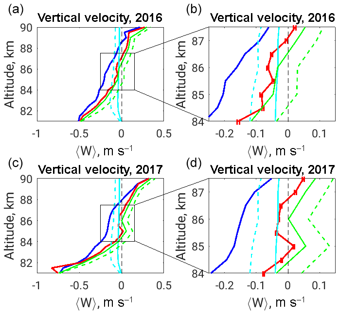
Figure 1Mean summer profiles for (blue) mean and (red) weighted mean vertical velocities, (dashed and solid light blue) sedimentation speed of ice spheres for two scenarios of their size distribution, and (dashed and solid green) results after eliminating ice sedimentation from weighted mean profiles. Panels (b) and (d) show increased version of the altitude range in black squares at panels (a) and (c) to highlight the error bars as uncertainties of the weighted mean values.
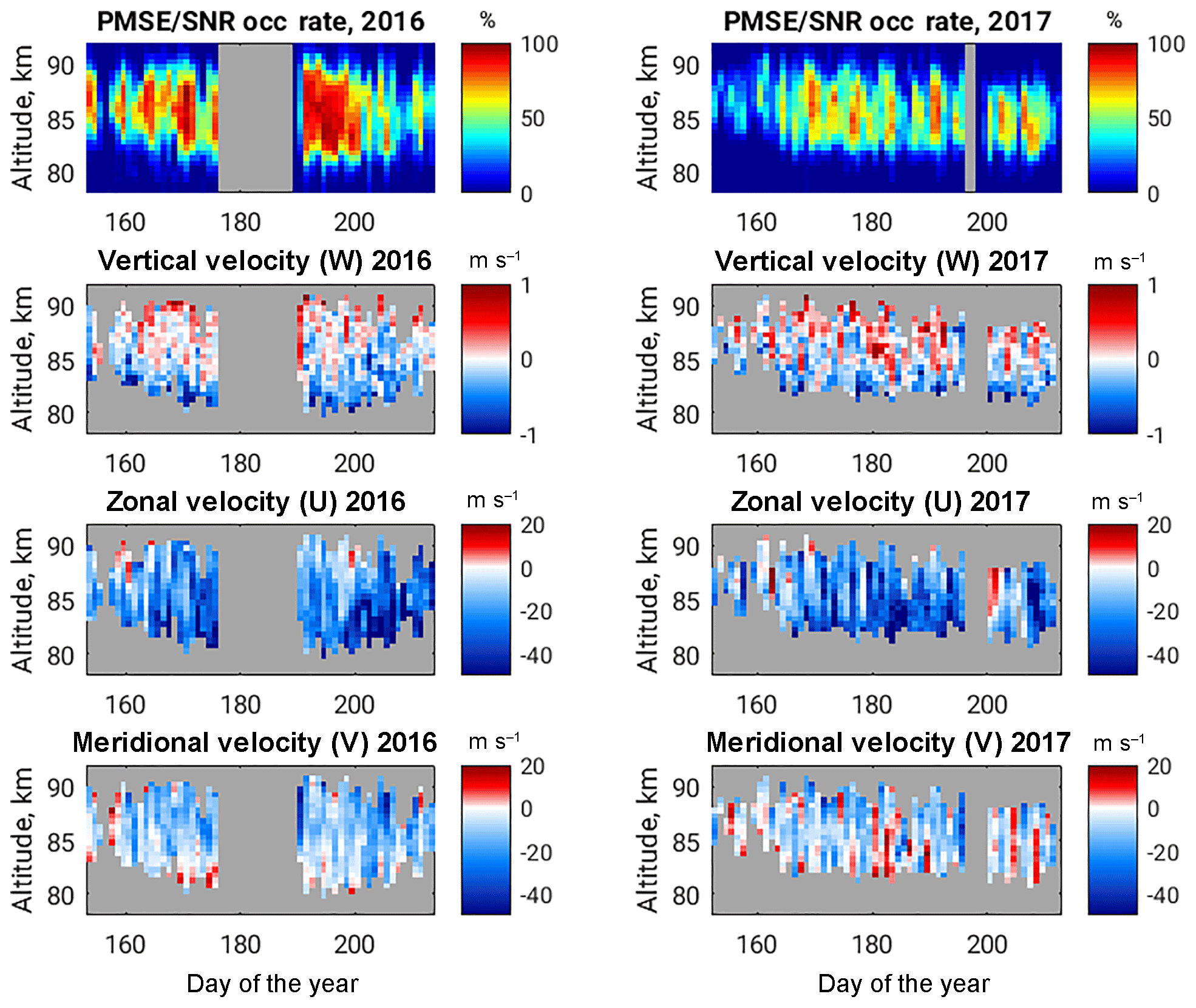
Figure 2Seasonal distribution of PMSE SNR diurnal occurrence rates (first row) and weighted mean diurnal profiles of vertical, zonal and meridional velocity vector components given in following rows. Positive values correspond to upward, eastward and northward directions. Velocity components correspond to those PMSE occurrences greater than 20 %. Grey colour indicates no data.
Weighted averages (solid red line) are characterised with different behaviour in three sections for both seasons. Vertically almost invariable values in the middle part between the ∼84 and 87 km altitude and the two outer sections have a sharp decrease and increase, respectively, at the lower and upper edges of the PMSE observable layer.
Weighted averages are presented as , where weights are and corresponding uncertainties of the averages will be .
To ensure statistically significant results, we filter the velocity measurements by PMSE occurrence. We averaged only those data at heights corresponding to the PMSE occurrence rates more than 20 %. The remaining data results in an average PMSE layer between the 81.5 and 89.5 km altitude in 2016 and between 82 and 89 km in 2017, considering the indicated threshold. The PMSE occurrence rate at a given altitude is a ratio of available data with the PMSE, defined by an SNR greater than −8 dB, to the full length of the observation time. We use this definition here and in the following plots as well. The weighted average values for the whole altitude range are −10 and −7 cm s−1 for the summers of 2016 and 2017, respectively. The simple mean values of observed vertical velocities, presented in the previous studies, were close to −20 cm s−1 (Balsley and Riddle, 1984; Meek and Manson, 1989; Fritts et al., 1990). We have also obtained similar mean values equal to downward 19 cm s−1 for both observed years.
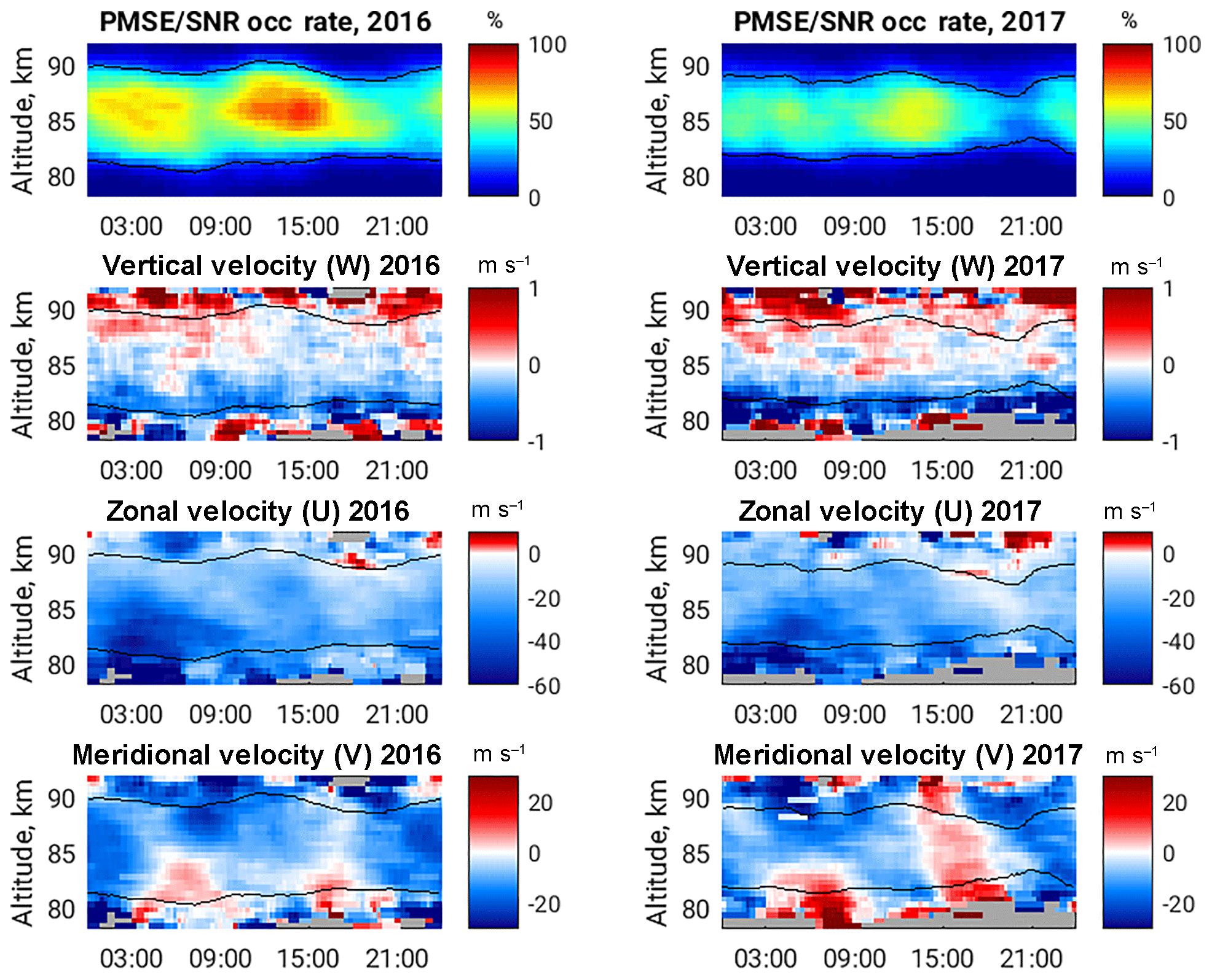
Figure 3Universal Time (UT) dependence of PMSE SNR occurrence rate (first row), and weighted mean diurnal profiles of vertical, zonal and meridional velocity vector components given on following rows. Positive values correspond to upward, eastward and northward directions respectively. Black solid contoured lines correspond to 20 % PMSE SNR occurrence rate; grey colour indicates no data.
However, due to the full error propagation, it is possible to weight all measurements with their corresponding statistical uncertainties, which is adequate, as larger velocities are often associated with larger errors and should be weighted correspondingly. Thus, the further discussion and presented results are weighted averages only. The terms “mean” or “average” regarding the vertical velocities should be understood as weighted averages.
Mean vertical velocities on Fig. 1 at altitudes above 87 km are strongly upward, while below 84 km they are downward with relatively high magnitudes, with values closer to zero between 84 and 87 km. Hence, it is more consistent to discuss each of the altitude sections separately, particularly as different physical processes related to the microphysics of the tracer are involved. We turn back to this in detail in the next section.
In spite of the seasonal mean distribution of the vertical velocities, considering the consistency of short time averages with the seasonal climatology is relevant. Daily distributions of the occurrence rates of the PMSE throughout the summer season and the altitude range between 78 and 92 km are shown in the uppermost panels of Fig. 2. The spatial distribution of the observed PMSE, as well as the seasonal occurrence, is in agreement with previous observations from the same location (Hoffmann et al., 1999; Latteck et al., 2008), which shows that the analysed two summer seasons are representative of a mean climatology.
The second panels of Fig. 2 show the colour-coded daily means of the observed vertical velocities corresponding to the occurrence of PMSE greater than 20 %. The main trend of the daily mean observed vertical motion below ∼87 km altitude is downward and is upward above it with negative and positive values, respectively. However, there are days with predominantly upward (e.g. the day of the year — DoY – of 173 in 2016 or a DoY of 183 in 2017) motion within the discussed altitude range. This contradicts the conclusion in the previous study by Hoppe and Fritts (1995b) that any mean vertical velocity observed with the PMSE should be biased toward downward behaviour. The tendency of a relatively strong downward shape below 84 km (dark blue colours) and weaker, close to zero values between 84 and 87 km altitudes (indicated as whitish) is also remarkable. In this way, the summer behaviour of the vertical velocity mainly corresponds to the mean seasonal profile shown in Fig. 1.
Seasonal distributions of daily mean values of zonal and meridional velocities over a given range of altitudes are plotted on the bottom two panels of Fig. 2. Shown summer climatology for both horizontal components agrees with those observed previously using meteor radars (Dowdy et al., 2007; Portnyagin et al., 2004; Wilhelm et al., 2017). In particular, the zonal wind shows a well-defined westward direction (here, negative values) and increases in magnitude at the lower altitudes. The meridional wind component tends to be equatorward (also negative values) but is weaker in magnitude than the zonal one. An expected tendency of seasonal behaviour is outlined; on the whole, however, the zonal wind reversal at the PMSE upper altitudes is rarely observed.
Figure 3 shows diurnal values of PMSE occurrence (upper panels) and PMSE velocity components – vertical, zonal and meridional, respectively, on the second, third and lower panels of the figure but averaged as a function of Universal Time (UT) and altitude. The half-hour temporal bins, with 10 min time step, are used to average all available velocity components at a given altitude.
We calculate the mean diurnal occurrence of the PMSE in the same way but look to the ratio of all available PMSE (SNR > −8 dB) within the given 30 min of each observed day to the full length of the measurements. The results are plotted on the upper panel on Fig. 3. The black contoured line indicates the PMSE occurrence equal to 20 %.
A significant increase in PMSE occurrence is observed during 12:00–16:00 UT, and a secondary peak is also noticeable in the early morning hours for both years. The similar behaviour of the PMSE occurrence was also reported in previous studies and was connected to the semidiurnal tidal variations (Hoffmann et al., 1999), but the diurnal production–reduction of electron densities is important too. Semidiurnal tidal behaviour is also significant in the horizontal wind components shown in the lower two panels of Fig. 3. However, the vertical velocity component (second panel) neither shows a clear dependence on the UT period nor on the PMSE strength. There is weak upward behaviour highlighted shortly at 06:00 UT for 2016 and after 09:00 UT for 2017 at around 85 km altitude, but the velocity values are mainly in good agreement with the mean seasonal profile.
We examined the mean vertical velocity dependence on PMSE strength as well as on Universal Time. The results show that the mean value of the vertical velocity and its altitude behaviour is not dependent on both mentioned parameters. The second and last columns of Fig. 4 show 2-D histograms as a function of the PMSE SNR and vertical velocity for the years 2016 and 2017, respectively. Typically we observe a symmetric Gaussian-like distribution for most of the PMSE strength values, except in some extreme cases where they are statistically sparse. The mean vertical profiles of vertical velocities shown in the panels to the left of the histograms correspond to the three separate intervals of PMSE strength. The lower corresponds to PMSE with an SNR larger than −8 dB but smaller than 5 dB; middle plots are done for velocities corresponding to a PMSE SNR between 5 and 20 dB, and the upper plots correspond to a PMSE SNR more than 20 dB. The behaviour of mean vertical velocity profile averaged at high PMSE values for summer 2017 is unlike all others because of lack of the relatively strong PMSEs during summer 2017. The difference is insignificant for the all other cases. No correlation between mean vertical velocity and PMSE strength is found, unlike previous reports based on several hours of measurements.
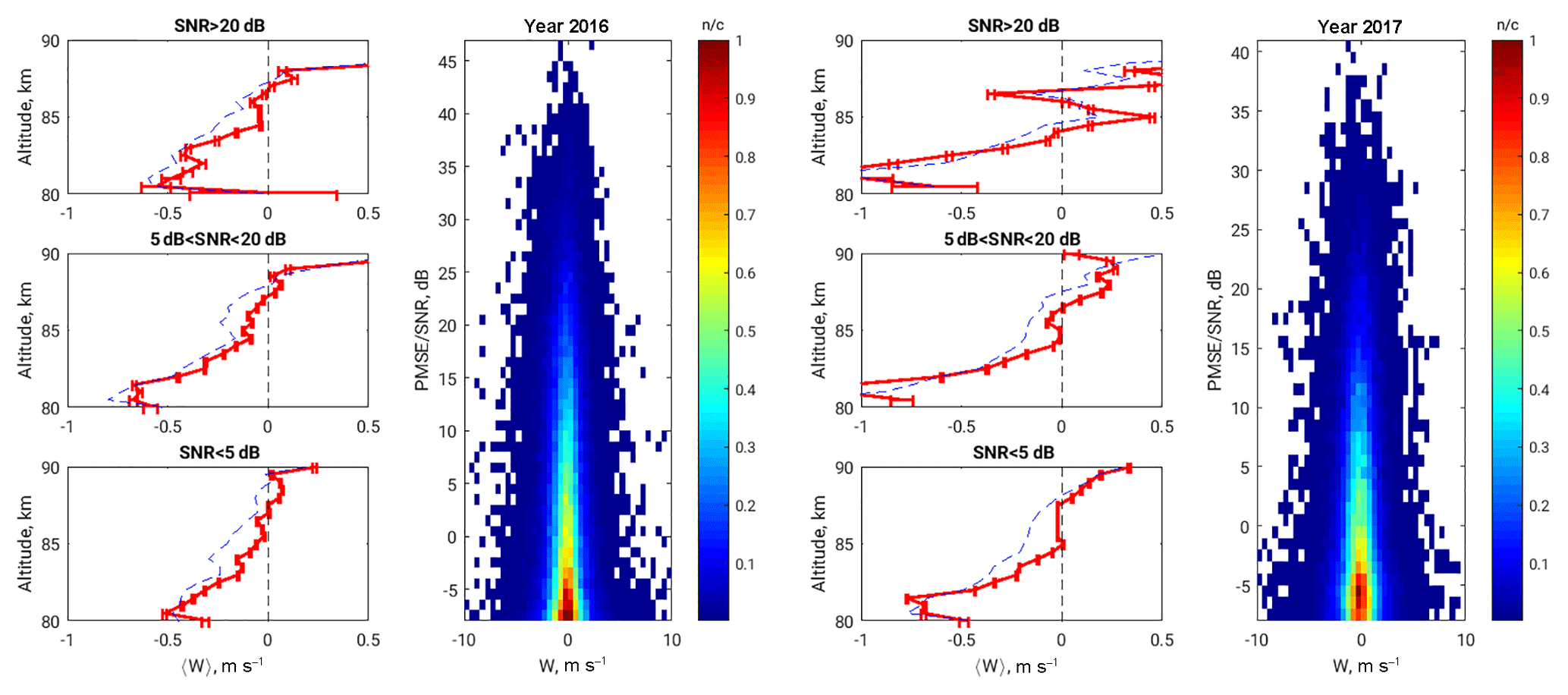
Figure 4Vertical profiles of weighted (red line) and simple (dashed blue line) mean vertical velocities corresponding to given range of PMSE SNR (first and third columns for summers of 2016 and 2017, respectively). 2-D histogram of vertical velocity measurements as a function of PMSE SNR (colour-coded panels).
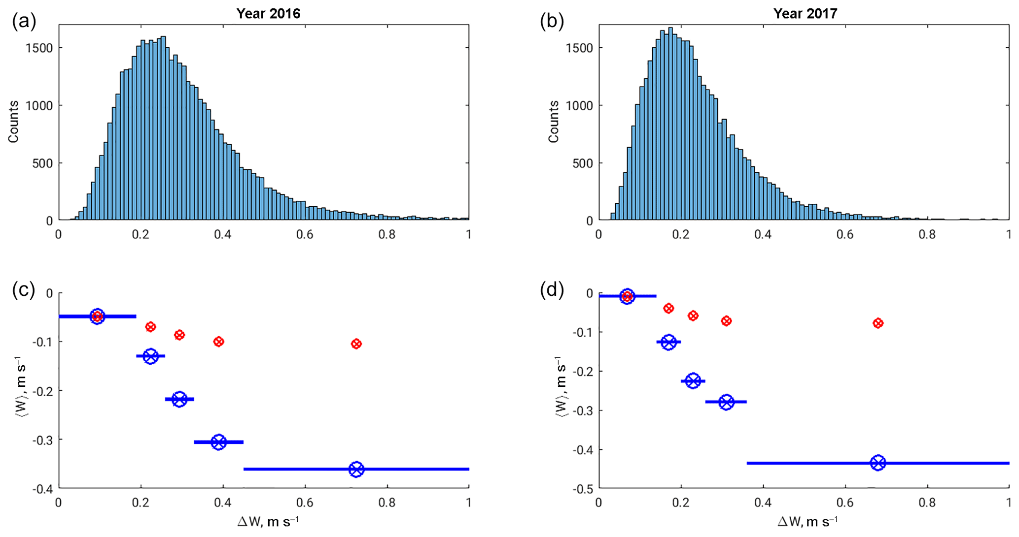
Figure 5(a, b) Histograms of vertical velocity uncertainties; (c, d) mean vertical velocity as a function of their uncertainties. Blue circles represent mean velocity values corresponding to velocity uncertainties, and range indicated with blue horizontal line on them. Ranges are divided equally with respect to similar data points for averaging. Red circles are mean vertical velocities for all those uncertainties lower than given point.
Outcomes from a given tracer indeed depend on the occurrence of given tracer. Results obtained from a tracer are acceptable if it appears randomly but not in certain circumstances associated with a background conditions. The reason for discrepancy of vertical velocity measurements in PMSE compared to the predictions from global circulation models has been explained by Hoppe and Fritts (1995b), who argued that the influence of background dynamics on appearance of PMSEs resulted in a bias on all measurements of vertical motion with radars. We discuss the presented mechanism first and return to our findings later.
Hoppe and Fritts (1995b) proposed a mechanism for the observed bias on the mean downward PMSE vertical velocity based on analysis of the 5 h PMSE (EISCAT – European Incoherent SCATter) radar measurements of the vertical beam radial velocity. They found that upward velocities that continued for more than 10 min led to increasing the variance of the motion field and tended to weaken PMSE. They concluded that the downward biases in PMSE mean vertical velocities are due to the gravity wave increasing the turbulence after a certain (upward) phase of the vertical motion field and made the PMSE appear weaker. The mean downward vertical velocities therefore correlated to the larger measurement uncertainties and variances in the low-pass filtered vertical motion field.
Large spectral width is usually an indicator of the strength of turbulence. The increase in variances of the radar Doppler velocities and measurement uncertainties is expected while observing the stronger turbulent air. The weakening of the PMSE at the large spectral width conditions is also known from the literature (Stober et al., 2018a; Chau et al., 2018). Hence, the explained mechanism of downward bias in PMSE vertical velocity is realistic. The question that remains is how systematic the described process is and how far it affects the seasonal climatology.
We investigated the correlation of the retrieved mean vertical velocity component in their statistical uncertainties for the summer seasons of both discussed years. The available data allow us to repeat only such correlation because of the difference in time resolution of datasets. The results are shown on Fig. 5. The histograms in the upper panels represent the distribution of measurement uncertainties Δw. The blue circles in the lower plots correspond to the vertical velocity mean values for only those measurements whose uncertainties are in the range marked by horizontal solid lines. Each “section” of uncertainties corresponds to the same amount of data points. The red circles show the mean of those vertical velocities corresponding to uncertainties lower than a given threshold. Therefore, Fig. 5 is the analogy of Fig. 4 in Hoppe and Fritts (1995b).
The result is opposite to that found by Hoppe and Fritts (1995b). Later we examined the resembling correlations concerning each available 6 h sections. Only a few cases, as shown by Hoppe and Fritts (1995b), were found with a positive correlation between mean downward values and uncertainties. Figure 6 shows such examples for both years. Following our results, we can summarise that the comprehensible dynamical process obtained from the relatively short period of observations can represent the localised event but might not be representative of an explanation of the climatology of vertical motion observed in the PMSE.
The time resolution of our dataset does not allow us to reexamine the mean vertical velocities as a function of variances on short-timescale motions. Nevertheless, to support our argument, we refer to Fig. 4. No clear evidence of dependence of vertical velocity distribution on PMSE strength is available from the seasonal 2-D histograms. However, the results of the vertical profiles of mean vertical velocity corresponding to different strength range of the PMSE are almost equal. The magnitude of mean downward values slightly changes at lower altitudes and middle strength of the PMSE but does not change at the central altitudes (84–87 km) of the PMSE occurrence, except those for SNR > 20 dB during the year 2017. This particular case is due to a small amount of the data points. In general, the PMSE in 2017 characterises weaker occurrence than during 2016 (upper panels of Figs. 2 and 3). We show that the seasonal climatology of the mean vertical velocities retrieved from the PMSE is not an evident function of the PMSE strength.
Figure 1 clearly shows the three well-developed sections of the mean vertical profile of the vertical velocity at PMSE altitudes. The central sections are downward but close to the zero values, with a mean equal to −7 and −2 cm s−1 in 2016 and 2017, respectively, between 84 and 87 km altitudes. Thus discussing the influence of sedimentation speed of ice particles on the measurements of PMSE radial velocities becomes substantial. The appearance of ice crystals with a charge attached to them is determinative for reduced electron diffusivity and creating radar backscatter in the presence of turbulence. Further, the ice particles are much heavier than the ambient atmosphere, and they sediment due to gravity. Such motion affects the vertical velocity measurements eventually. According to the present knowledge of the mesospheric ice physics, those particles can be created at PMSE altitudes where the atmospheric temperature can reach below the frost point (Lübken and von Zahn, 1991; Lübken, 1999; Rapp and Lübken, 2004) for the typical mixing ratios of the water vapour (Garcia, 1989).
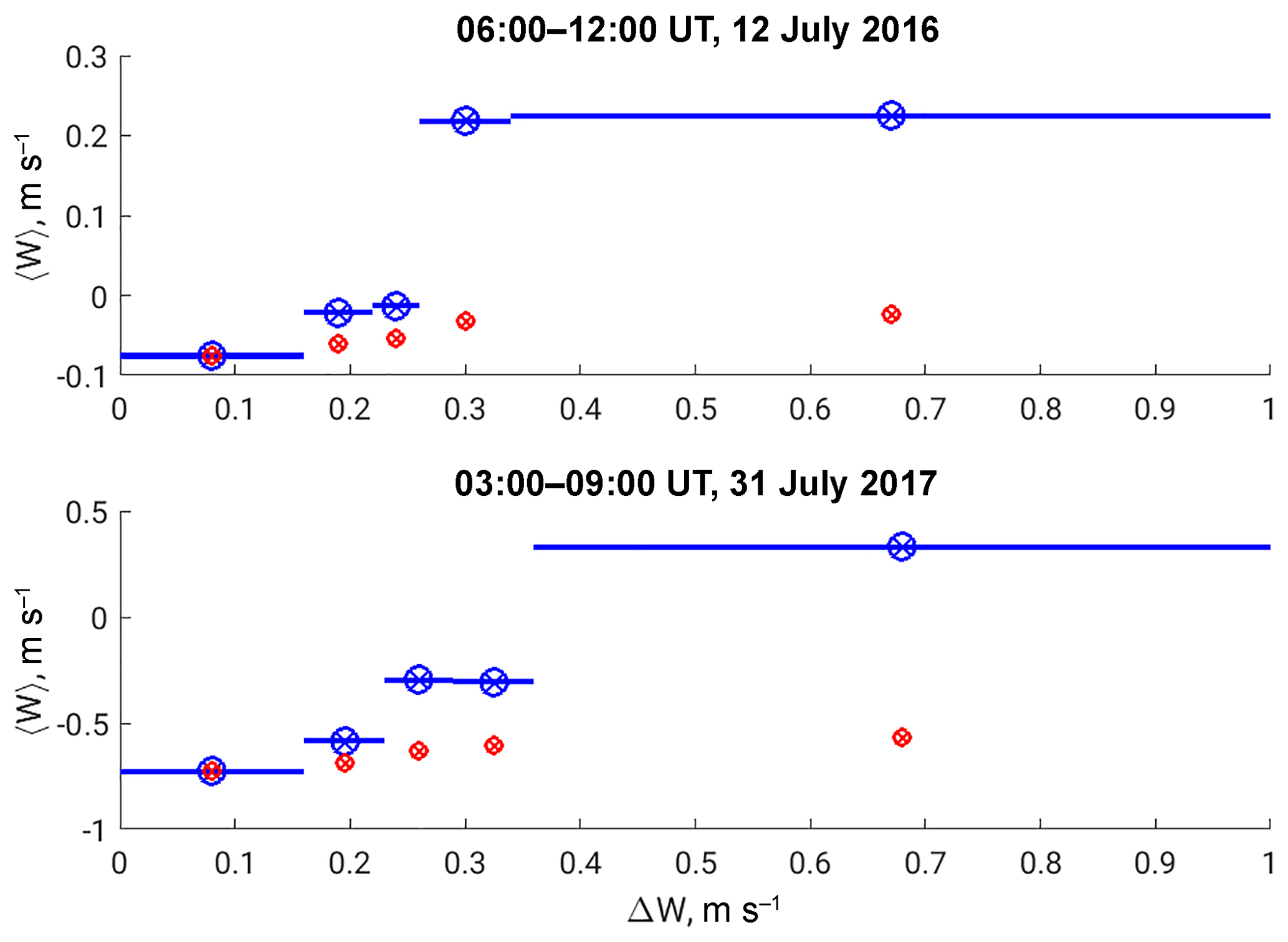
Figure 6Couple of examples of positive correlation between mean vertical velocities and their uncertainties as shown by Hoppe and Fritts (1995b). The exact time intervals are indicated on the plots. Further details can be found in the text.
Ice particles are sedimenting slowly downward. The sedimentation velocity depends on the size and shape of the particles as well as the ambient atmospheric density. We now discuss the possibility of using the PMSE as an inert tracer to obtain realistic vertical velocities in the summer mesosphere but not present the quantitative analysis here. Hence, we take into account the idealised case, when ice crystals have a spherical form. Following Reid (1975) the falling velocity of such ice particles is
where ρ is the density, r is the radii of the falling sphere, g is the acceleration due to gravity, n is the number density, T is the absolute temperature of the air, k is Boltzmann's constant and m is a mass of the air molecules. Mean summer air number density and temperature profiles are taken from the NRLMSISE-00 model (Picone et al., 2002) for summer 2016 and applied for both discussed years due to the availability of model outputs. The mean mass of the molecule is calculated as a weighted mass based on the densities of main constituents ([O], [O2] and [N2]) at the mesospheric altitudes. We use 910 kg m−3 as the ice mass density, ρ. We consider two scenarios of the radii r distribution. One follows Berger and Lübken (2015), who modelled the ice formation and growth to derive the expected particle sizes at different altitudes. It results in ice spheres from 5 to ∼35 nm from the altitude range of 90 down to 82 km and a rapid decrease to a few nanometres at the lower altitudes. Observations sometimes show the NLC with the ice particles in 100 nm (von Cossart et al., 1999). Therefore the second scenario considers the extreme size distribution of ice grains from 10 to 100 nm at the above-mentioned altitudes.
The results are plotted in a light blue colour in Fig. 1 (all panels) as the solid and dashed lines corresponding to the first and second scenarios. Green solid and dashed lines on the same plots represent the corrected observed mean velocities (red curve) after eliminating the influence of ice falling speed (e.g. ). The resulted velocities became upward for both years after excluding the effect from the ice descend with expected magnitudes in range of few centimetres per second at the discussing altitudes of high PMSE occurrence (84–87 km). We argue that this result can be understood as clear evidence of direct observation of the mean upwelling in the summer mesosphere. Also, the PMSE can be discussed as an inert tracer for the vertical neutral wind but only at the certain altitudes.
In the previous section, we have proposed the relevance of discussing the observed and/or retrieved vertical velocities separately at the middle and outer altitudes of PMSE occurrence. The evidence of the sharp increase and/or decrease in the summer mean vertical velocity at the edges above 87 and below 84 km in Fig. 1 should have a separate explanation.
The vertical motion activity in the region as well as in the atmosphere can be a result of wave propagation, created turbulence due to shear instability, or a result of gravity wave breaking (Hecht et al., 2000). Such disturbances indeed transport air masses on the corresponding scales. Relatively large-scale motions are usually accompanied with short-scale wave processes. The effect of the ambient air motion on the PMSE is widely observed and can be explained as ice clouds following the atmospheric behaviour.
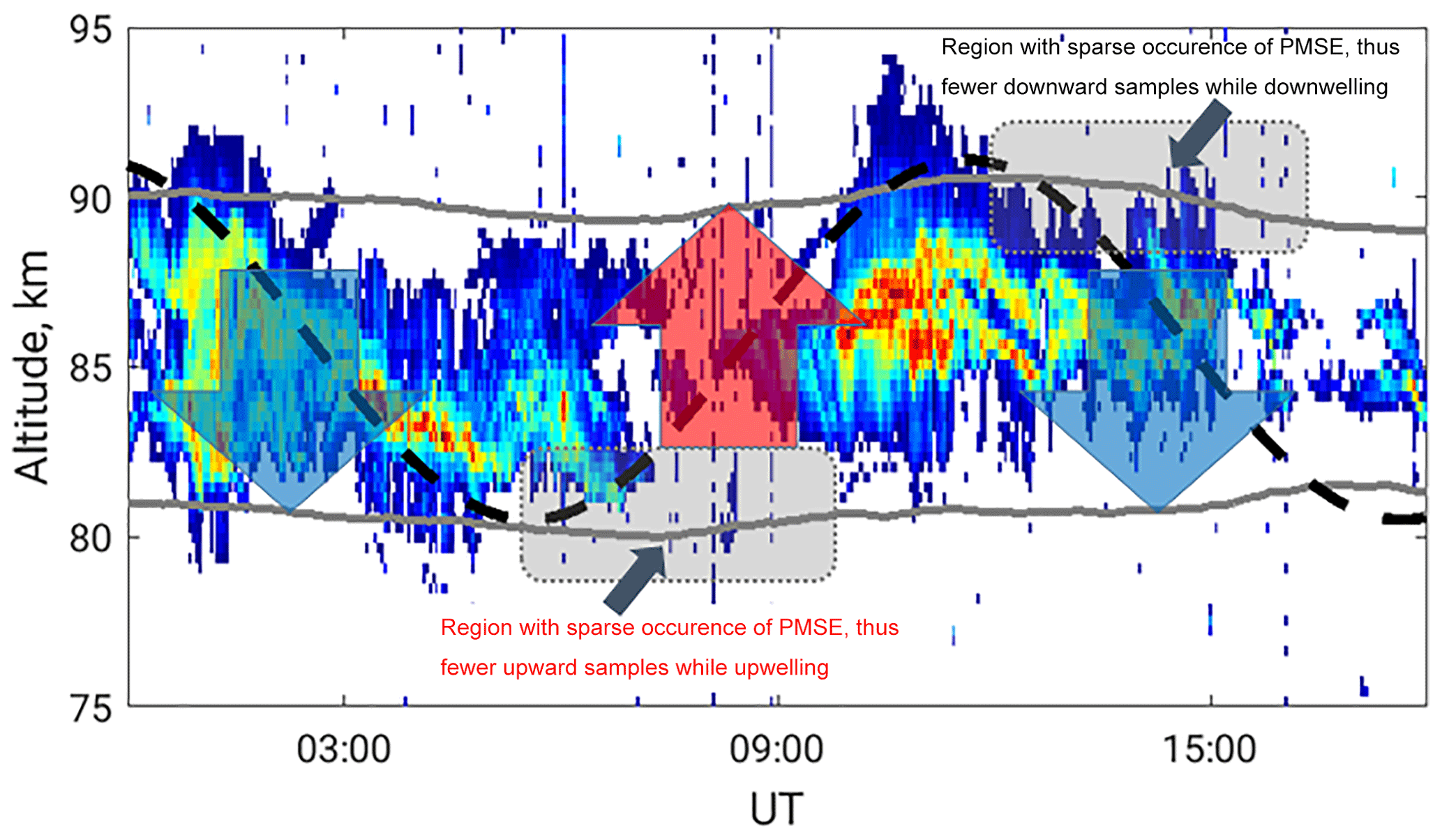
Figure 7Example of typical PMSE structure observed on 29 July 2016, and sketch of idealised propagated sinusoidal wave at PMSE altitudes. Arrows indicate the upward or downward phase of the wave. Colour-coded PMSE is thresholded at SNR of −8 dB. Thus, white background corresponds to no data. Grey line shows boundaries of seasonal average of diurnal PMSE occurrence more than 20 %. The sketch highlights sampling issues of PMSE and Doppler velocity measurements on the edges.
A typical day, as an example of PMSE temporal behaviour, is shown in Fig. 7. Static ground-based measurements are not capable of observing intrinsic motion but look in the specific fixed volume in the atmosphere. Hence, the horizontal transport of the tracer is also essential for describing the observed vertical fluctuations. The large-scale gravity waves generated and transported from the lower altitudes have a characteristic vertical wavelength of 15–20 km at upper mesospheric altitudes (Mitchell and Howells, 1998; Schmidt et al., 2018). The upwelling or downwelling phase of such motion exceeds the width of the PMSE layer and is capable of transporting air masses from lower or upper heights where the ice clouds and PMSE are not present.
We plot the idealised sinusoidal wave sketch in Fig. 7 as the black dashed line. The beginning phase at ∼ 01:00–05:00 UT corresponds to the downward motions, and PMSE structures follow the air to the lower altitudes. There they disappear due to melting, sublimation or horizontal advection which moves in air masses without the PMSE. The measured Doppler velocities are only available as long as the radar detects the echo. The uprising phase of the vertical component of a propagating wave starts after ∼ 05:00 UT (for the given example), and, due to the missing PMSE at the lower altitudes, the evidence of upward vertical motions is under-represented in the measurements. Following the progress, the temporal evolution shows that horizontal transport is important, as later the PMSE is advected again into the observed volume. However, at the central altitudes of the PMSE layer, it was again possible to obtain vertical velocities.
The similar but opposite picture with respect to the motion direction is evident at the upper edge (close to and after ∼ 10:00 UT in Fig. 7). Finally, the number of data points with downward motions are dominant at the lower altitudes, and correspondingly there is an excess of upward velocity measurements at the upper or top heights. The effect is more evident when the distance from the PMSE central altitudes is considered. Here we proposed a geophysical explanation of the sharp trends at the edges of the vertical profile of the mean vertical velocity retrieved from five-beam PMSE Doppler velocities.
We present a climatology of PMSE (polar mesospheric summer echo) mean vertical velocities at polar mesospheric altitudes for two summer seasons. The main objective of this study was a detailed analysis and understanding of these velocities, since previous studies have shown that they are not in agreement with the expected upwelling in the MLT (mesosphere–lower thermosphere) due to the residual circulation.
Our results indicate that continuous 3-D wind measurements are necessary for deriving a mean vertical motion in the MLT from PMSE observations. The PMSE can be considered to be an inert but not a passive tracer. As a result, reliable climatologies are only obtained at altitudes with a 24 h PMSE coverage. Further, we have to consider that the charged aerosols inside the PMSE reduce the electron diffusivity and are basically sedimenting with the ice particles. Taking into account such expected sedimentation speeds, the weighted mean vertical velocity in the central region of PMSE altitudes (i.e. 84–87 km) shows a small upward motion. Such upward motion is in agreement with that predicted and expected for the polar summer mesosphere.
However, at the upper and lower edges of the PMSE layer, the weighted mean vertical velocities show unexpected behaviour. They tend to be upward or downward at upper or lower edges. We proposed that this behaviour is due to the non-uniform appearance of PMSEs in altitude and time. For example, an upward velocity is not picked up by the measurements at the lower altitudes, since no PMSE can be advected from below the PMSE layer, while during downward motion, the PMSE is basically advected from the altitudes above, and the tracer disappears merely after melting the remaining ice particles. A reversed effect occurs on the upper edge of the layer. Horizontal advection of the PMSE plays an important role at the middle altitudes where the ratio of upward and downward measurements becomes independent of the phase of vertical motion field.
We also examined the possible biases on the PMSE vertical velocity measurements from certain phases of short-period gravity waves previously proposed by Hoppe and Fritts (1995b). Based on the statistical analysis of the available long dataset, we found that the mean behaviour of PMSE vertical velocity does not depend on the PMSE brightness at altitudes between 84 and 87 km, where we found a sufficient high occurrence rate. No positive correlation between downward velocities and velocity uncertainties were found as well. We argue that the results of short-time measurements cannot be extrapolated to climatological behaviour.
MAARSY PMSE wind data are available upon request (stober@iap-kborn.de).
NG provided the data analysis. The raw data were processed by GS. The work is supervised by JLC. All authors contributed to the editing of the paper.
The authors declare that they have no conflict of interest.
This article is part of the special issue “Layered phenomena in the mesopause region (ACP/AMT inter-journal SI)”. It is a result of the LPMR workshop 2017 (LPMR-2017), Kühlungsborn, Germany, 18–22 September 2017.
Authors acknowledge helpful discussion with Gerd Baumgarten. The work was
supported by the WaTiLa project
(SAW-2015-IAP-1).
The publication of this
article was funded by the
Open Access Fund of the Leibniz
Association.
This paper was edited by William Ward and reviewed by two anonymous referees.
Balsley, B. B. and Riddle, A. C.: Monthly Mean Values of the Mesospheric Wind Field over Poker Flat, Alaska, J. Atmos. Sci., 41, 2368–2380, https://doi.org/10.1175/1520-0469(1984)041<2368:MMVOTM>2.0.CO;2, 1984. a, b, c, d
Baumgarten, G. and Fritts, D. C.: Quantifying Kelvin-Helmholtz instability dynamics observed in noctilucent clouds: 1. Methods and observations, J. Geophys. Res.-Atmos., 119, 9324–9337, https://doi.org/10.1002/2014JD021832, 2014. a
Becker, E.: Dynamical Control of the Middle Atmosphere, Space Sci. Rev., 168, 283–314, https://doi.org/10.1007/s11214-011-9841-5, 2012. a, b
Berger, U. and Lübken, F.-J.: Trends in mesospheric ice layers in the Northern Hemisphere during 1961–2013, J. Geophys. Res.-Atmos., 120, 11277–11298, https://doi.org/10.1002/2015JD023355, 2015. a
Chau, J. L. and Kudeki, E.: First E- and D-region incoherent scatter spectra observed over Jicamarca, Ann. Geophys., 24, 1295–1303, https://doi.org/10.5194/angeo-24-1295-2006, 2006. a
Chau, J. L., McKay, D., Vierinen, J. P., La Hoz, C., Ulich, T., Lehtinen, M., and Latteck, R.: Multi-static spatial and angular studies of polar mesospheric summer echoes combining MAARSY and KAIRA, Atmos. Chem. Phys., 18, 9547–9560, https://doi.org/10.5194/acp-18-9547-2018, 2018. a, b
Cho, J. Y. N. and Röttger, J.: An updated review of polar mesosphere summer echoes: Observation, theory, and their relationship to noctilucent clouds and subvisible aerosols, J. Geophys. Res.-Atmos., 102, 2001–2020, https://doi.org/10.1029/96JD02030, 1997. a
Coy, L., Fritts, D. C., and Weinstock, J.: The Stokes Drift due to Vertically Propagating Internal Gravity Waves in a Compressible Atmosphere, J. Atmos. Sci., 43, 2636–2643, https://doi.org/10.1175/1520-0469(1986)043<2636:TSDDTV>2.0.CO;2, 1986. a
Czechowsky, P. and Rüster, R.: VHF radar observations of turbulent structures in the polar mesopause region, Ann. Geophys., 15, 1028–1036, https://doi.org/10.1007/s00585-997-1028-8, 1997. a
Czechowsky, P., Rüster, R., and Schmidt, G.: Variations of mesospheric structures in different seasons, Geophys. Res. Lett., 6, 459–462, https://doi.org/10.1029/GL006i006p00459, 1979. a
Dowdy, A., Vincent, R. A., Igarashi, K., Murayama, Y., and Murphy, D. J.: A comparison of mean winds and gravity wave activity in the northern and southern polar MLT, Geophys. Res. Lett., 28, 1475–1478, https://doi.org/10.1029/2000GL012576, 2001. a
Dowdy, A. J., Vincent, R. A., Tsutsumi, M., Igarashi, K., Murayama, Y., Singer, W., and Murphy, D. J.: Polar mesosphere and lower thermosphere dynamics: 1. Mean wind and gravity wave climatologies, J. Geophys. Res.-Atmos., 112, D17104, https://doi.org/10.1029/2006JD008126, 2007. a
Ecklund, W. L. and Balsley, B. B.: Long-term observations of the Arctic mesosphere with the MST radar at Poker Flat, Alaska, J. Geophys. Res.-Space, 86, 7775–7780, https://doi.org/10.1029/JA086iA09p07775, 1981. a
Fauliot, V., Thuillier, G., and Vial, F.: Mean vertical wind in the mesosphere-lower thermosphere region (80–120 km) deduced from the WINDII observations on board UARS, Ann. Geophys., 15, 1221-1231, https://doi.org/10.1007/s00585-997-1221-9, 1997. a
Fiedler, J., Baumgarten, G., Berger, U., Hoffmann, P., Kaifler, N., and Lübken, F.-J.: NLC and the background atmosphere above ALOMAR, Atmos. Chem. Phys., 11, 5701–5717, https://doi.org/10.5194/acp-11-5701-2011, 2011. a
Fritts, D., Hoppe, U.-P., and Inhester, B.: A study of the vertical motion field near the high-latitude summer mesopause during MAC/SINE, J. Atmos. Terr. Phys., 52, 927–938, https://doi.org/10.1016/0021-9169(90)90025-I, 1990. a, b
Fritts, D. C., Baumgarten, G., Wan, K., Werne, J., and Lund, T.: Quantifying Kelvin-Helmholtz instability dynamics observed in noctilucent clouds: 2. Modeling and interpretation of observations, J. Geophys. Res.-Atmos., 119, 9359–9375, https://doi.org/10.1002/2014JD021833, 2014. a
Garcia, R. R.: Dynamics, Radiation, and Photochemistry in the Mesosphere: Implications for the Formation of Noctilucent Clouds, J. Geophys. Res., 94, 14, 605–614, https://doi.org/10.1029/JD094iD12p14605, 1989. a
Garcia, R. R. and Solomon, S.: The effect of breaking gravity waves on the dynamics and chemical composition of the mesosphere and lower thermosphere, J. Geophys. Res.-Atmos., 90, 3850–3868, https://doi.org/10.1029/JD090iD02p03850, 1985. a, b
Gerding, M., Zöllner, J., Zecha, M., Baumgarten, K., Höffner, J., Stober, G., and Lübken, F.-J.: Simultaneous observations of NLCs and MSEs at midlatitudes: implications for formation and advection of ice particles, Atmos. Chem. Phys., 18, 15569–15580, https://doi.org/10.5194/acp-18-15569-2018, 2018. a
Hall, T. M., Cho, J. Y. N., Kelley, M. C., and Hocking, W. K.: A re-evaluation of the Stokes drift in the polar summer mesosphere, J. Geophys. Res.-Atmos., 97, 887–897, https://doi.org/10.1029/91JD02835, 1992. a
Hecht, J. H., Fricke-Begemann, C., Walterscheid, R. L., and Höffner, J.: Observations of the breakdown of an atmospheric gravity wave near the cold summer mesopause at 54N, Geophys. Res. Lett., 27, 879–882, https://doi.org/10.1029/1999GL010792, 2000. a
Hervig, M. E., Gerding, M., Stevens, M. H., Stockwell, R., Bailey, S. M., Russell, J. M., and Stober, G.: Mid-latitude mesospheric clouds and their environment from SOFIE observations, J. Atmos. Sol.-Terr. Phy., 149, 1–14, https://doi.org/10.1016/j.jastp.2016.09.004, 2016. a
Hoffmann, P., Singer, W., and Bremer, J.: Mean seasonal and diurnal variations of PMSE and winds from 4 years of radar observations at ALOMAR, Geophys. Res. Lett., 26, 1525–1528, https://doi.org/10.1029/1999GL900279, 1999. a, b
Holton, J. R.: The role of gravity wave induced drag and diffusion in the momentum budget of the mesosphere, J. Atmos. Sci., 39, 791–799, https://doi.org/10.1175/1520-0469(1982)039<0791:TROGWI>2.0.CO;2, 1982. a, b
Holton, J. R. and Alexander, M. J.: The Role of Waves in the Transport Circulation of the Middle Atmosphere, in: Atmospheric Science Across the Stratopause, Geophys Monograph: 123, American Geophysical Union (AGU), 21–35, https://doi.org/10.1029/GM123p0021, 2013. a
Hoppe, U.-P. and Fritts, D. C.: High-resolution measurements of vertical velocity with the European incoherent scatter VHF radar: 1. Motion field characteristics and measurement biases, J. Geophys. Res., 100, 16813–16825, https://doi.org/10.1029/95JD01466, 1995a. a, b, c
Hoppe, U.-P. and Fritts, D. C.: On the downward bias in vertical velocity measurements by VHF radars, Geophys. Res. Lett., 22, 619–622, https://doi.org/10.1029/95GL00165, 1995b. a, b, c, d, e, f, g, h, i
Kiliani, J., Baumgarten, G., Lübken, F.-J., Berger, U., and Hoffmann, P.: Temporal and spatial characteristics of the formation of strong noctilucent clouds, J. Atmos. Sol.-Terr. Phy., 104, 151–166, https://doi.org/10.1016/j.jastp.2013.01.005, 2013. a
Kirkwood, S., Nilsson, H., Morris, R. J., Klekociuk, A. R., Holdsworth, D. A., and Mitchell, N. J.: A new height for the summer mesopause: Antarctica, December 2007, Geophys. Res. Lett., 35, L23810, https://doi.org/10.1029/2008GL035915, 2008. a
Kudeki, E., Bhattacharyya, S., and Woodman, R. F.: A new approach in incoherent scatter F region E×B drift measurements at Jicamarca, J. Geophys. Res.-Space, 104, 28145–28162, https://doi.org/10.1029/1998JA900110, 1999. a
Laskar, F. I., Chau, J. L., St.-Maurice, J. P., Stober, G., Hall, C. M., Tsutsumi, M., Höffner, J., and Hoffmann, P.: Experimental Evidence of Arctic Summer Mesospheric Upwelling and Its Connection to Cold Summer Mesopause, Geophys. Res. Lett., 44, 9151–9158, https://doi.org/10.1002/2017GL074759, 2017. a
Latteck, R., Singer, W., Morris, R. J., Hocking, W. K., Murphy, D. J., Holdsworth, D. A., and Swarnalingam, N.: Similarities and differences in polar mesosphere summer echoes observed in the Arctic and Antarctica, Ann. Geophys., 26, 2795–2806, https://doi.org/10.5194/angeo-26-2795-2008, 2008. a, b
Latteck, R., Singer, W., Rapp, M., Vandepeer, B., Renkwitz, T., Zecha, M., and Stober, G.: MAARSY: The new MST radar on Andøya – System description and first results, Radio Sci., 47, RS1006, https://doi.org/10.1029/2011RS004775, 2012. a
Lindzen, R. S.: Turbulence and Stress Owing to Gravity Wave and Tidal Breakdown, J. Geophys. Res., 86, 9707–9714, https://doi.org/10.1029/JC086iC10p09707, 1981. a, b
Lübken, F.-J.: Thermal structure of the Arctic summer mesosphere, J. Geophys. Res.-Atmos., 104, 9135–9149, 1999. a, b
Lübken, F.-J. and von Zahn, U.: Thermal structure of the mesopause region at polar latitudes, J. Geophys. Res.-Atmos., 96, 20841–20857, https://doi.org/10.1029/91JD02018, 1991. a
Meek, C. E. and Manson, A. H.: Vertical Motions in the Upper Middle Atmosphere from the Saskatoon (52∘ N, 107∘ W) M.F. Radar, J. Atmos. Sci., 46, 849–859, https://doi.org/10.1175/1520-0469(1989)046<0849:VMITUM>2.0.CO;2, 1989. a
Mitchell, N. J. and Howells, V. St. C.: Vertical velocities associated with gravity waves measured in the mesosphere and lower thermosphere with the EISCAT VHF radar, Ann. Geophys., 16, 1367–1379, https://doi.org/10.1007/s00585-998-1367-0, 1998. a
Nastrom, G. D. and VanZandt, T. E.: Mean Vertical Motions Seen by Radar Wind Profilers, J. Appl. Meteorol., 33, 984–995, https://doi.org/10.1175/1520-0450(1994)033<0984:MVMSBR>2.0.CO;2, 1994. a
Picone, J. M., Hedin, A. E., Drob, D. P., and Aikin, A. C.: NRLMSISE-00 empirical model of the atmosphere: Statistical comparisons and scientific issues, J. Geophys. Res.-Space, 107, 1468, https://doi.org/10.1029/2002JA009430, 2002. a
Portnyagin, Y., Solovjova, T., Merzlyakov, E., Forbes, J., Palo, S., Ortland, D., Hocking, W., MacDougall, J., Thayaparan, T., Manson, A., Meek, C., Hoffmann, P., Singer, W., Mitchell, N., Pancheva, D., Igarashi, K., Murayama, Y., Jacobi, C., Kuerschner, D., Fahrutdinova, A., Korotyshkin, D., Clark, R., Taylor, M., Franke, S., Fritts, D., Tsuda, T., Nakamura, T., Gurubaran, S., Rajaram, R., Vincent, R., Kovalam, S., Batista, P., Poole, G., Malinga, S., Fraser, G., Murphy, D., Riggin, D., Aso, T., and Tsutsumi, M.: Mesosphere/lower thermosphere prevailing wind model, Adv. Space Res., 34, 1755–1762, https://doi.org/10.1016/j.asr.2003.04.058, 2004. a
Rapp, M. and Lübken, F.-J.: Polar mesosphere summer echoes (PMSE): Review of observations and current understanding, Atmos. Chem. Phys., 4, 2601–2633, https://doi.org/10.5194/acp-4-2601-2004, 2004. a, b, c, d
Rapp, M., Strelnikova, I., Latteck, R., Hoffmann, P., Hoppe, U.-P., Häggström, I., and Rietveld, M. T.: Polar mesosphere summer echoes (PMSE) studied at Bragg wavelengths of 2.8 m, 67 cm, and 16 cm, J. Atmos. Sol.-Terr. Phy., 70, 947–961, https://doi.org/10.1016/j.jastp.2007.11.005, 2008. a
Reid, G. C.: Ice clouds at the summer polar mesopause, J. Atmos. Sci., 32, 523–535, https://doi.org/10.1175/1520-0469(1975)032<0523:ICATSP>2.0.CO;2, 1975. a
Schmidt, C., Dunker, T., Lichtenstern, S., Scheer, J., Wüst, S., Hoppe, U.-P., and Bittner, M.: Derivation of vertical wavelengths of gravity waves in the MLT-region from multispectral airglow observations, J. Atmos. Sol.-Terr. Phy., 173, 119–127, https://doi.org/10.1016/j.jastp.2018.03.002, 2018. a
Sheth, R., Kudeki, E., Lehmacher, G., Sarango, M., Woodman, R., Chau, J., Guo, L., and Reyes, P.: A high-resolution study of mesospheric fine structure with the Jicamarca MST radar, Ann. Geophys., 24, 1281–1293, https://doi.org/10.5194/angeo-24-1281-2006, 2006. a
Smith, A.: Global Dynamics of the MLT, Surv. Geophys., 33, 1177–1230, https://doi.org/10.1007/s10712-012-9196-9, 2012. a
Sommer, S., Stober, G., Chau, J. L., and Latteck, R.: Geometric considerations of polar mesospheric summer echoes in tilted beams using coherent radar imaging, Adv. Radio Sci., 12, 197–203, https://doi.org/10.5194/ars-12-197-2014, 2014. a
Sommer, S., Stober, G., and Chau, J. L.: On the angular dependence and scattering model of polar mesospheric summer echoes at VHF, J. Geophys. Res.-Atmos., 121, 278–288, https://doi.org/10.1002/2015JD023518, 2016. a, b
Stober, G., Sommer, S., Rapp, M., and Latteck, R.: Investigation of gravity waves using horizontally resolved radial velocity measurements, Atmos. Meas. Tech., 6, 2893–2905, https://doi.org/10.5194/amt-6-2893-2013, 2013. a
Stober, G., Chau, J. L., Vierinen, J., Jacobi, C., and Wilhelm, S.: Retrieving horizontally resolved wind fields using multi-static meteor radar observations, Atmos. Meas. Tech., 11, 4891–4907, https://doi.org/10.5194/amt-11-4891-2018, 2018a. a, b, c
Stober, G., Sommer, S., Schult, C., Latteck, R., and Chau, J. L.: Observation of Kelvin–Helmholtz instabilities and gravity waves in the summer mesopause above Andenes in Northern Norway, Atmos. Chem. Phys., 18, 6721–6732, https://doi.org/10.5194/acp-18-6721-2018, 2018b. a, b, c
von Cossart, G., Fiedler, J., and von Zahn, U.: Size distributions of NLC particles as determined from 3-color observations of NLC by ground-based lidar, Geophys. Res. Lett., 26, 1513–1516, https://doi.org/10.1029/1999GL900226, 1999. a
Wilhelm, S., Stober, G., and Chau, J. L.: A comparison of 11-year mesospheric and lower thermospheric winds determined by meteor and MF radar at 69∘ N, Ann. Geophys., 35, 893–906, https://doi.org/10.5194/angeo-35-893-2017, 2017. a