the Creative Commons Attribution 4.0 License.
the Creative Commons Attribution 4.0 License.
 | 04 Apr 2019
An evaluation of the efficacy of very high resolution air-quality modelling over the Athabasca oil sands region, Alberta, Canada
Matthew Russell
Amir Hakami
Paul A. Makar
Ayodeji Akingunola
Junhua Zhang
Michael D. Moran
Qiong Zheng
We examine the potential benefits of very high resolution for air-quality forecast simulations using a nested system of the Global Environmental Multiscale – Modelling Air-quality and Chemistry chemical transport model. We focus on simulations at 1 and 2.5 km grid-cell spacing for the same time period and domain (the industrial emissions region of the Athabasca oil sands). Standard grid cell to observation station pair analyses show no benefit to the higher-resolution simulation (and a degradation of performance for most metrics using this standard form of evaluation). However, when the evaluation methodology is modified, to include a search over equivalent representative regions surrounding the observation locations for the closest fit to the observations, the model simulation with the smaller grid-cell size had the better performance. While other sources of model error thus dominate net performance at these two resolutions, obscuring the potential benefits of higher-resolution modelling for forecasting purposes, the higher-resolution simulation shows promise in terms of better aiding localized chemical analysis of pollutant plumes, through better representation of plume maxima.
- Article
(5478 KB) - Companion paper
- BibTeX
- EndNote


Numerical modelling of the atmosphere in an Eulerian framework relies on discretization of the computational domain into a numerical grid. The horizontal grid-cell size of atmospheric simulations can range from hundreds of kilometres to the metre-scale of large eddy simulation models. Air-quality model grid-cell size typically follows the grid-cell sizes used in weather forecasting models, which in turn have followed a gradual progression towards finer discretization where more explicit representation of cloud formation and local radiative transfer effects may be represented. The most recent weather forecasting applications (e.g. Leroyer et al., 2014) have reached grid-cell sizes as small as 250 m over limited domains such as individual cities, and have shown promising results in terms of being able to resolve some aspects of local circulation. In addition, as grid resolution reaches the 3 to 4 km scale, explicit cloud microphysics packages may be used, allowing potentially better performance, particularly with regards to feedbacks between meteorology and chemistry (Yu et al., 2014; Gong et al., 2015). However, while these models promise better physical representation of local chemistry, their performance may be limited by the quantity and availability of initialization and boundary condition meteorological data; these data may be used in a data assimilation context to improve their initial state. The accuracy of broader-scale meteorological predictions may thus influence local model accuracy, despite the ongoing decrease in meteorological model (and consequently air-quality model) grid-cell size. Some recent air-quality model simulation studies with grid-cell sizes on the order of 1 to 4 km include Thompson and Selin (2012), Li et al. (2014), Joe et al. (2014), Kheirbek et al. (2014, 2016), and Pan et al. (2017).
For the purposes of this study, very high resolution (VHR) modelling refers to the current higher-resolution limits of chemical transport models (CTMs), employing a horizontal grid-cell spacing of 1 km or less. It is in this regime that the photochemical processes may be forecasted with resolved microphysics (e.g. Milbrandt and Yau, 2005a, b) and detailed particle and gas-phase chemistry, using currently available computer technology. VHR modelling is very computationally expensive, and also introduces its own set of challenges, such as the availability of surface boundary condition fields as the model grid-cell size decreases. Moreover, it is not currently clear whether decreases in model grid-cell size leads to more accurate results when compared to observations. The motivation behind VHR modelling in CTMs is to reduce the impact of diluting chemical concentrations – especially from averaging emission plumes into large grid cells – in order to better capture inhomogeneities in emission profiles, to better simulate local transport processes associated with terrain that would otherwise be smoothed by the use of a coarse grid, and to reduce truncation errors and hence achieve better numerical accuracy (Jacobson, 1999).
We note here that while the terms “grid-cell size” and “resolution” tend to be used interchangeably in the literature, this is not true in a precise mathematical sense; more formally, the ability to resolve features of size 2Δx requires a grid-cell spacing of size Δx, and the highest spatial frequency which can be reconstructed from a discrete sampling of the latter grid-cell spacing will be , the Nyquist wavenumber of the grid-cell size discretization. Furthermore, atmospheric models may make use of energy dissipation techniques that broaden the size of resolvable wavelengths to 3 to 4 Δx (Grasso, 2000; Pielke, 2001). Model resolution is thus a function of, but not equivalent to, grid-cell size. Here, we define “resolution” as the ability of a model to clearly distinguish components of a predicted atmospheric variable, as a function of grid-cell size.
The issue of a model to distinguish these features is also compounded by uncertainties in model inputs. For example, in a large rural setting, a large model grid cell will represent an area containing many roads, whose emissions will be averaged into one value per species per time. As the grid-cell size decreases, however, this averaging effect will be reduced, giving each road's emissions more impact on the resulting concentrations in the grid cell containing it. However, the smaller grid-cell size will also result in steeper concentration gradients in the model between adjacent grid cells, which can in turn result in numerical instabilities that contaminate predictions (Salvador et al., 1999). At the same time, a reduction in grid-cell size can be shown formally to reduce inaccuracies in the discretization of the governing equations for atmospheric motion (Coiffier, 2011). Previous efforts to address these issues through variable grid size or structure in air quality modelling have not received sustained attention, and therefore most current air quality models use a uniform (albeit nested) grid-cell size in applications (Garcia-Menendez et al., 2010; Kumar et al., 1997).
As resolution increases further, the presence of local topographical features (e.g. buildings and street canyons) becomes more important. Both the increased topographic complexity and potential numerical instabilities can lead to differences in meteorological forcing as resolution increases (Wolke et al., 2012; Gego et al., 2005). The contribution of meteorological uncertainties due to resolution becomes more significant, especially for secondary pollutants such as ozone (Valari and Menut, 2008) or secondary particulate matter (PM). For example, Markakis et al. (2015) in their analysis of 4 km CHIMERE simulations for the relatively flat terrain of Paris, France, suggested that model meteorological grid-cell size does not significantly impact forecast accuracy. That may not have been the case, had their terrain been more complex. In contrast, Queen and Zhang (2008) observed considerable meteorological sensitivity to the more complex terrain in their 4 km resolution Community Multiscale Air Quality (CMAQ; EPA, 1999) model simulations over the Appalachian Mountains in the eastern United States, as did Salvador et al. (1999) for meteorological model simulations.
A number of studies have tried to evaluate the benefits of higher-resolution simulations and to quantify the impact of sub-grid variability by using different model grid-cell sizes (Vardoulakis et al., 2003; Ching et al., 2006; Pepe et al., 2016). These studies have often demonstrated that failure to account for higher-resolution features may result in mischaracterization of concentrations or health impacts (Isakov et al., 2007), although the capability of current models to provide this information with sufficient accuracy is unclear. One study found that increasing resolution did not change predicted health outcomes and concluded that “resolution requirements should be assessed on a case-by-case basis” (Thompson and Selin, 2012), while others (e.g. Kheirbek et al., 2014, 2016) have employed 1 km resolution without discussing the impacts of resolution on predicted health outcomes. Population exposure studies using air pollution models may be affected by resolution in a more complex fashion, given that both the predicted field (a pollutant with a known health impact) and the data to which the predicted field is to be linked (the human population) both have resolution dependencies. The health studies carried out to date highlight the need for better understanding of the underlying controlling factors for model accuracy with decreasing grid-cell size.
Terrain and meteorology are not the only factors that contribute to greater uncertainties as horizontal grid-cell size is reduced – for example, the ability of the model to locally resolve emission fluxes may also become a factor. This may result in improved or deteriorated model performance as the size of the grid cells decreases. Gridded model emissions may have an intrinsic resolution dependence due to the underlying spatial disaggregation fields, and this can contribute to uncertainties and errors in emissions as grid-cell size is decreased. For instance, Valari and Menut (2008) found that the discrepancy between their modelled and observed concentrations grew rather than shrank, in response to decreases in grid-cell size from 48 to 6 km, and they associated these results with changes in the resulting local emission fluxes. They showed that in their model setup, with regard to ozone, a grid-cell size was reached (12 km × 12 km) where errors in inputs (errors in the emission inventory, wind direction, etc.) outweighed the importance of other sources of model error such as grid-cell size. The authors, however, noted that Paris' ozone photochemistry very often resides on the transition between a -sensitive and a VOC-sensitive regime (Sillman et al., 2003). These are chemical conditions which can alternatively produce or titrate ozone and hence have a degree of sensitivity to precursor emissions, and therefore, also, to any errors in those emissions. Conversely, in a 3-level nested MM5–CMAQ simulation with grid-cell sizes going from 9 to 3 to 1 km over Osaka, Japan, Shrestha et al. (2009) found that ozone comparisons to observations improved as the grid resolution increased. This was also the case for a 3-level nested MM5–CMAQ simulation going from 36 to 12 to 4 km over Houston, USA (Ching et al., 2006), where the ozone forecast improvement associated with higher resolution was attributed to the ability of the finer grid-cell size model nests to adequately resolve high concentrations of freshly emitted NOx and hence allow for more local ozone titration. The latter process might not take effect until the grid-cell size is sufficiently fine to resolve the NOx source patterns (i.e. a level where traffic and industrial sources can be identified.) This titration was not seen until they decreased their grid-cell sizes to 2 km and smaller. Stroud et al. (2011) noted a similar grid-cell-size-dependent chemical impact on model performance, where secondary organic aerosol formation maxima were better simulated with a 2.5 km grid-cell size model than a 10 km grid-cell size model. In general, the impact of resolution on model performance appears to depend on a number of factors, such as the terrain, spatial distribution of sources, pollutant of concern, season, etc. (Arunachalam et al., 2006; Queen and Zhang, 2008; Dore et al., 2012).
Salvador et al. (1999) studied the prediction accuracy impacts of meteorological model grid-cell size in a region with a complex domain and found that 2 km or smaller grid-cell sizes were required to resolve local-scale complex terrain flow features, and that daytime vertical advection and predictions of turbulent kinetic energy and potential temperature were influenced by grid-cell size. Dore et al. (2012) evaluated air quality model NO2 simulations employing 1, 5, and 50 km grid-cell sizes against observations and found the best performance for the 1 km simulation, with more physically realistic distributions of reactive nitrogen, attributing this performance gain to more realistically precipitation simulations and emissions inputs for the smallest grid-cell size. The availability of high-resolution emissions information may be a limiting factor in improved simulations as grid-cell size decreases. Valari and Menut (2008) noted that emissions inaccuracy was the principal cause of noise in small grid-cell size simulations conducted for the Paris area, and proposed the use of statistical downscaling in favour of predictive modelling at scales at or below 1 km grid-cell size. The current state of model science is typically evaluated through multi-model intercomparisons (e.g. Im et al., 2015), and the meta-analysis of these studies can be used to provide useful benchmarks to assess current model performance for specific model species and observations (Emery et al., 2017). However, such studies do not identify the causes for good or poor performance relative to the benchmarks – diagnostic studies “in which chemical and physical processes within the model are analyzed individually and collectively” (Emery et al., 2017) are required for this purpose. Examinations of the impact of model grid-cell size on performance are an example of such a diagnostic evaluation.
The benefits for model performance with increased spatial resolution are unclear, based on the above literature. However, most papers converge towards the following qualitative conclusions:
-
The impact of terrain topology on meteorological forcing as grid-cell size decreases can dwarf the impact of a more accurate spatial apportionment of the corresponding emissions.
-
Decreases in grid-cell size result in a more realistic spatial distribution of chemical species, whether or not model performance is improved.
-
Uncertainties in spatial and temporal emissions allocation have an increasing influence on overall model uncertainty as model grid-cell size decreases.
The 1980s saw several studies in which the potential impacts of wind direction errors on dispersion model performance were examined. Fox (1981) noted that pairing of model output at observation station locations could be done as a function of both time and space: as a function of time (by combining the data across all stations), as a function of space (by combining all times, at each station location), or without any pairing (observations and data were compared as cumulative frequency distributions). The accuracy of regulatory dispersion models in the early 1980s was such that Fox (1984) concluded that model and observation values paired in time and space exhibited “little to no correlation” and discussed potential errors associated with transport. Poor correlations were also noted in the report on the first generation of reactive-transport models by Hanha (1988), who stated “wind direction errors are the major cause of the poor agreement in hourly predictions of concentrations at short distances downwind of point sources,” and described metrics for air-quality model evaluation. Hanha (1988) also noted that model predictions could be offset in space and time relative to observations, leading to poor performance statistics, despite a greater degree of similarity of behaviour if the offsets are taken into account. Errors in wind-field modelling were described as the main source of error in simulations of plumes by Carhart et al. (1989), who again showed how better agreement resulted when model and observations were unpaired in time and/or space and noted that other metrics such as maximum plume width might better represent model performance. Lee (1987) found that small perturbations in space and time could result in poor correlations, despite similar histogram distributions of both model and observations.
More recently, Kang et al. (2007) examined the concept of using the area of the limiting resolution of the model (2 to 3Δx, where Δx is the horizontal grid-cell size) to weight or spatially average model evaluation metrics for a single grid-cell size, noting how the model's rated ability to capture high-concentration events (“hits”) was increased when the limiting resolution of the model was incorporated into the performance metrics. However, the use of averaging may mask the potential for a model with a small grid-cell size to contain both the desired plume magnitude and much lower concentrations, within the same larger representative area, in turn masking the potential impact of the reduction in grid-cell size.
We expand on this concept to evaluate the impact of model grid-cell size in the context of an equivalent area about a given observation location. We examine area-weighted metrics in the form of averages over roughly equivalent areas for different model grid-cell sizes, and also use the a priori knowledge of the observations to determine whether the closest match to observations may be found within an equivalent area. We show that the latter metric demonstrates a positive impact of model grid-cell size on simulation results, while more simple paired comparisons, and averages over similar areas, mask these benefits.
We examine the impact of grid-cell size on model performance in a region of intense petrochemical extraction and upgrading, the Athabasca oil sands region (AOSR). The AOSR refers to the northernmost of three large bitumen deposits located the northern part of the province of Alberta in Canada: the Athabasca, Peace River, and Cold Lake areas. Together these areas cover 142 200 km2 in total and constitute the third largest oil reserves in the world (Government of Alberta, 2016), as shown in Fig. 1. The oil sands sector is the second largest source of SO2 and the third largest source of industrial NOx in the province of Alberta. This sector is also a significant source of industrial PM, CO, and volatile organic compound (VOC) emissions (Zhang et al., 2018), from a variety of source types and industrial processes (e.g. open pit mine tailings ponds, large diesel fleets, bitumen upgrading facilities). As is described below, very high resolution emissions data are available for these sources, and emissions take place in a region with significant topography, hence the region provides a good test case for the relative impact of grid-cell size on air-quality model prediction results.
Next we describe our model, the simulation domains and forecasting setup, the emissions data, our evaluation methodology, and the results of our analysis.
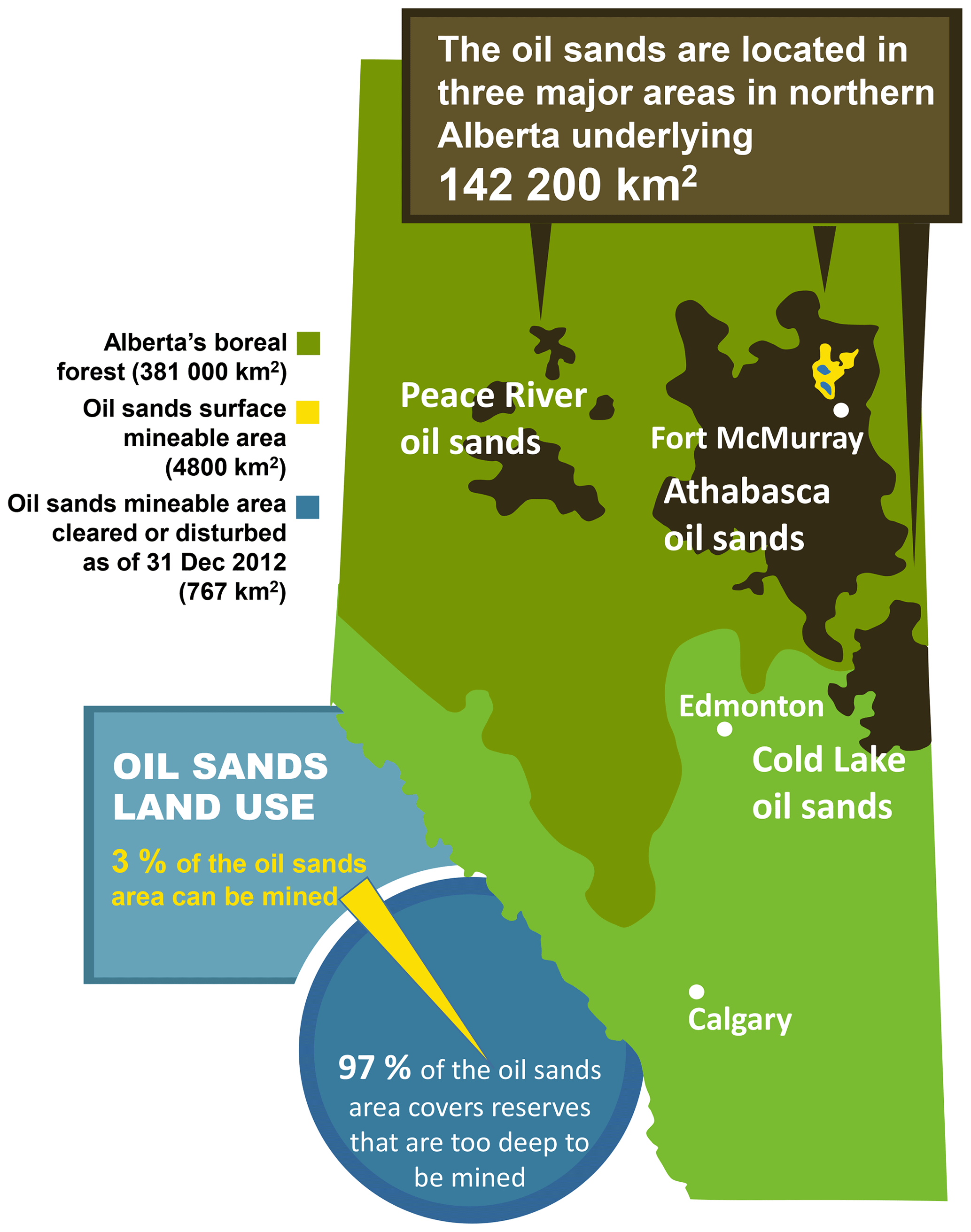
Figure 1Map showing the oil sands regions (based on an image from Government of Alberta, 2016).
2.1 GEM-MACH
The air-quality model used in this work is Environment and Climate Change Canada's (ECCC) Global Environmental Multiscale – Modelling Air-quality and Chemistry (GEM-MACH) model, which has been in use as Canada's operational air-quality forecast model since 2009 (Moran et al., 2010). GEM-MACH is an on-line model; that is, both meteorological and chemistry processes are handled within a single model. The chemical processes reside within the physics module of the Global Environmental Multiscale meteorological forecast model (Côté et al., 1998a, b), originate with Environment Canada's earlier off-line model (A Unified Regional Air-quality Modelling System, AURAMS; Gong et al., 2006), and include process representation for particle microphysics (Gong et al., 2003a, b), inorganic heterogeneous chemistry (Makar et al., 2003), aqueous phase chemistry, in-cloud and below-cloud scavenging (Gong et al., 2006), and secondary organic aerosol formation (Stroud et al., 2011). GEM-MACH employs a sectional approach to represent the size distribution of atmospheric particles, with 12-bin (Makar et al., 2015a, b; Gong et al., 2015) or 2-bin configurations (Moran et al., 2010). The latter configuration is designed for maximum computational efficiency, with re-binning to the 12-bin distribution for key particle microphysics processes, in order to improve accuracy. Here, the 2-bin version of the model has been used, the main focus of the work being the impact of horizontal grid-cell size on model results. Eight aerosol chemical components are resolved in GEM-MACH (sulfate, nitrate, ammonium, elemental carbon, primary organic aerosol, secondary organic aerosol, sea salt, and crustal material). In the present study, we make use of GEM-MACH v.1.5.1, described in more detail in Makar et al. (2015a, b), employing 80 levels in a hybrid vertical coordinate system extending up to 0.1 hPa (∼30 km). Both model grid-cell size simulations compared here (2.5 and 1 km grid-cell sizes; see below) make use of the Milbrandt–Yau double-moment explicit microphysics scheme; that is, cloud processes are resolved explicitly at these scales (Milbrandt and Yau, 2005a, b).
2.2 Model setup
2.2.1 Grid nesting
Four levels of nesting have been employed in our simulations, shown in Fig. 2a. This version of GEM-MACH operates on a rotated latitude–longitude coordinate system wherein the position of the coordinate system poles is set by the user, allowing rotations of the grid with decreasing grid-cell size during nesting. The outermost nested grid corresponds to the westernmost two-thirds of the operational GEM-MACH forecasting domain, with a 10 km grid-cell size, and employ a combination of the Kain–Fritsch sub-gridscale convective cloud scheme (Kain and Fritsch, 1990; Kain, 2004) and a Sunqvist (1988) scheme for cloud parameterizations. Within that outer grid is nested a 10 km grid-cell size western Canada domain (yellow region, Fig. 2a) which has been rotated to match the horizontal orientation of the Rocky Mountains, and which makes use of a double-moment microphysics scheme (Milbrandt and Yau, 2005a, b) in place of the Sundqvist (1988) parameterization. The intention of this intermediate local 10 km simulation domain was to provide initial hydrometeors for the two innermost domains, to reduce the “spin-up” time required for the inner domains' meteorology to reach an equilibrium with respect to cloud formation. The latter two domains (2.5 and 1 km grid-cell sizes) resolve the cloud microphysics explicitly using the double-moment scheme alone and no convective parameterization (Milbrandt and Yau, 2005a, b). The third nested grid inset (green region, Fig. 2a) is the 2.5 km grid-cell size domain, which covers most of the Canadian provinces of Alberta and Saskatchewan. This grid will hereafter be referred to as the OS2.5km domain. The fourth and final nested grid (blue square, Fig. 2a) is a 1 km grid-cell size domain, roughly centered over and covering the immediate environs of the Athabasca oil sands, and is referred to hereafter as the OS1km model. This last nest also shows the region within which 22 instrumented aircraft flights were conducted during August and September of 2013, providing a unique measurement data set for our evaluation of the OS2.5 and OS1km model output for the same time period. Table 1 provides details on the horizontal dimensions of each of these nested domains and the duration of the simulations on each grid. All four model nests make use of the same vertical coordinate and levels. Figure 2b shows the topography of the 1 km domain in detail; the region to be modelled is situated in a broad river valley, with a local vertical relief of 750 m. Significant wind shears and frequent inversions are observed in the region, and part of our interest in 1 km grid-cell size simulations is to determine the extent to which these local features may influence model prediction accuracy.
2.2.2 Simulation cycling strategy
Model simulations mimic an operational forecasting system, starting from the use of archived, data-assimilated meteorological analyses as meteorological input and boundary conditions every 36 h. The use of analysis fields is a standard meteorological forecasting practice to prevent the chaotic drift of the model results from observed meteorology over time. The outermost 10 km domain uses initial and boundary conditions from the output of a meteorological simulation, that is itself driven by an analysis field. The outermost domain model then carries out a 36 h forecast, of which the first 6 h is discarded as spin-up; the final 30 h is used as initial and boundary conditions for the rotated 10 km grid-cell size domain (the OS10 km domain). An OS10 km simulation of 30 h is then carried out, with the first 6 h being discarded as spin-up, and the latter 24 h forming the initial and boundary conditions for the 2.5 km grid-cell size OS2.5km simulation. The OS2.5km simulation is of 24 h duration. The OS1km simulation covers the same 24 h (and hence both 2.5 and 1 km simulations start from the same OS10 km initial conditions for every 24 h forecast), with the 2.5 km simulation providing boundary conditions thereafter to the OS1km model. Continuity between 24 h forecasts is thus maintained at the level of the outermost nest. The outermost domain is cycled every 12 h starting at 00:00 and 12:00 UT; however, we have selected the set of contiguous OS2.5 and OS1km 24 h simulations starting from the 12:00 UT continental domain for our comparison.
Meteorological boundary conditions for the lowest-resolution GEM-MACH simulations are taken from operational GEM forecasts, in turn driven by data assimilation analyses performed at the Canadian Meteorological Centre.
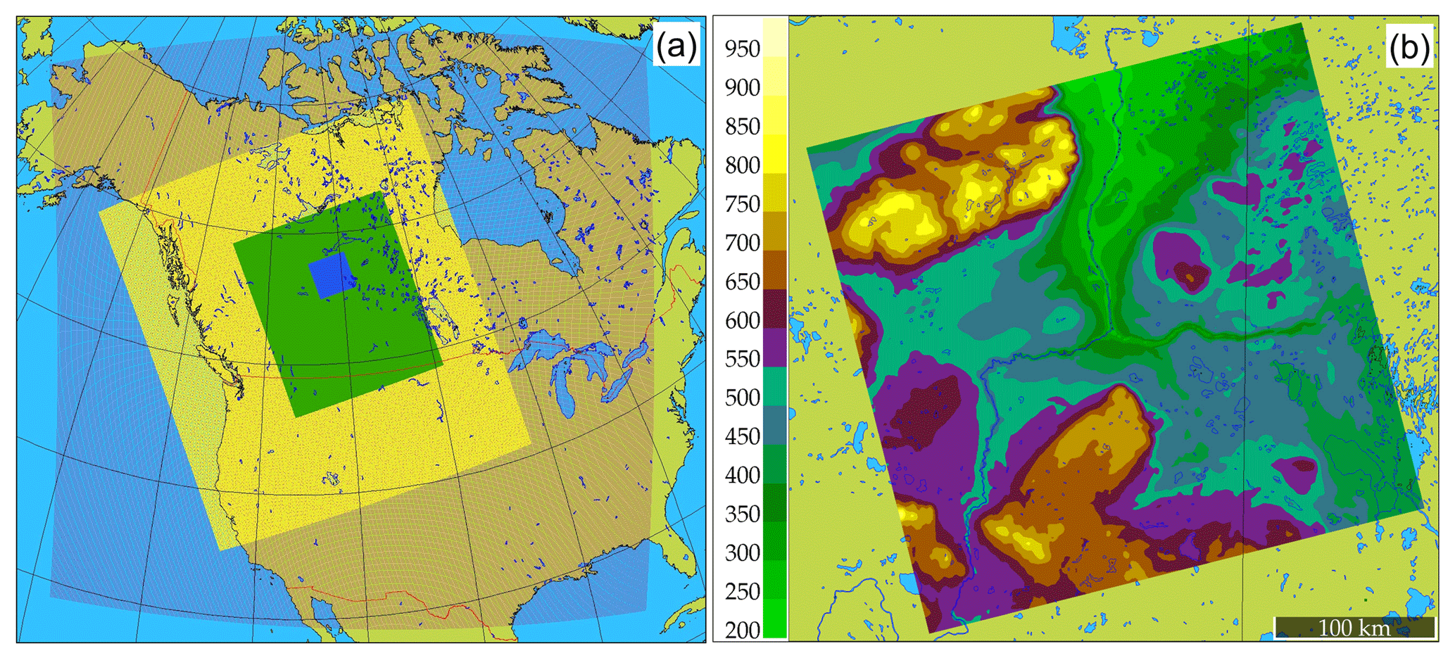
Figure 2(a) The four nested domains of the GEM-MACH simulations. From outermost to innermost domains, these are CONT10 km (outermost, red dots), OS10 km (yellow), OS2.5km (green), and OS1km (blue). The model simulations from the two innermost domains are the focus of the present study. (b) Topography in the OS1km domain centered on Fort McMurray, Alberta (m a.g.l.). The coloured area corresponds to the central blue domain in (a).
Table 1Nested domain specifications.
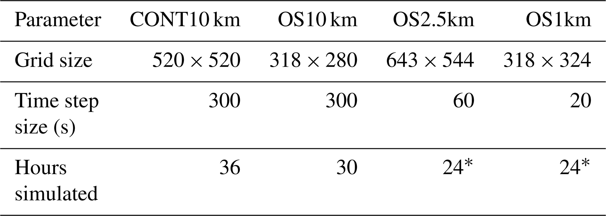
* Note that both OS2.5 and OS1km output frequency was hourly.
2.3 Model emissions
All emissions data used in this work are described in Zhang et al. (2018). These emissions data include
- a.
direct observations of stack-specific hourly emissions measured by continuous emission monitoring systems (CEMS);
- b.
regional emissions inventory data from the Cumulative Environmental Management Association (CEMA) – which had the most detailed stack and process level emission data for the AOSR facilities, including emissions from mine faces, tailings ponds, and the off-road mining feet);
- c.
the 2010 Canadian Air Pollutant Emissions Inventory (APEI) – which is the most comprehensive national emissions inventory, and which has the largest spatial coverage for area sources outside the AOSR; and
- d.
the 2013 National Pollutant Release Inventory (NPRI) (a subset of the APEI) that is based on emissions reports from large industrial facilities.
These emissions data sets primarily describe emissions of pollutants known as criteria air contaminants (NOx, VOCs, SO2, NH3, CO, PM2.5, and PM10) for major-point sources (i.e. large emission stacks) and area sources. Area emissions sources typically consist of multiple small mobile sources spread over a large area (e.g. off-road vehicles), large flux sources such as mine tailings settling ponds or mine faces, and/or large numbers of small stacks for which no stack characteristic data (volume flow rates, temperatures of emissions, stack diameters), needed to estimate plume-rise heights, are available.
Major-point sources are represented by a single geographical (latitude, longitude) pair of coordinates, and are assigned to the grid cell in which the point is located. These sources are likely to be the most impacted by model horizontal grid-cell size, as even a large major-point source plume, which in reality may only occupy an emissions horizontal area on the order of 100 m2, is represented by a flux spread over an entire grid cell. A plume from a major point source within a 2.5 km grid cell will thus be immediately diluted to a size of 6.25 km2 upon emission, whereas the same source with a 1 km grid cell will have a cross-sectional horizontal extent of 1 km2. At the same time, higher resolution may require a much more accurate representation of model winds close to the sources to maintain accuracy in evaluation metrics dependant on plume position such as correlation – a wider plume being more likely to at least partially intersect a monitoring station location than a narrower plume.
Area sources that are large compared to both model grid-cell sizes (2.5 and 1 km) can be expected to be approximated by model grid cells of both resolutions and are thus expected to be less impacted by model resolution than emissions from point sources. However, smaller area sources (i.e. areas intermediate between 2.5 and 1 km to the side) may be better resolved, and hence have less dilution and higher downwind concentrations, when higher spatial resolution is employed.
In the AOSR, approximately 95 % of the SO2 emissions originate in major-point sources, while NO2 is apportioned ∼40 % to major-point sources and ∼60 % to area sources (Zhang et al., 2018). Consequently our a priori expectation is that the impact of the resolution change will be strongest for species like SO2, and less strong for species like NO2 that are emitted in part by point sources, but may also be apparent for other species and secondary products, such as O3.
2.4 Model evaluation methodology and metrics
Comparisons between air-quality models and observations usually take the approach of comparing observation and model-generated values paired in time and space, from the observation location and corresponding model grid-cell respectively. We refer to this approach hereafter as our “standard” evaluation, for both 2.5 and 1 km simulations. However, we note additional factors aside from grid-cell size may influence the outcome of air-quality model evaluations. For example, the relative skill of the meteorological component of the air-quality model will depend in part on the density of meteorological observation data, incorporated into the model via data assimilation, for the construction of the model's initial meteorological state. This in turn will influence the local skill of the model's predicted wind directions and hence the skill of its plume transport. The simulations carried out here focus on the Fort McMurray area, where the nearest available upper air meteorological sounding site is located at the ECCC Stony Plain station, located approximately 500 km south-west of the study area. The advantage of higher-resolution simulations (e.g. reduced numerical error associated with the discretization of transport operators, and better treatment of local topographic influences) may thus be offset by errors in the predicted large-scale flow.
While meteorological model synoptic-scale forecast errors may manifest themselves locally as errors in the direction of winds driving local plume transport, other advantages may result from the use of higher-resolution air-quality models. Since lower resolution models de facto instantaneously redistribute plumes emitted from large stack sources over a larger area, such artificial diffusion will reduce the model's ability to accurately simulate concentration maxima, and the resulting chemistry, within simulated model plumes. However, the spatial extent of a plume in a model employing a large horizontal grid-cell size may be such that its existence may be captured at discrete observing sites. In contrast, forecast plumes in models with smaller horizontal grid-cell sizes may correctly capture plume magnitude and chemical behaviour, but may be more subject to errors in the larger-scale wind direction. To illustrate this point, Fig. 3 shows a conceptual diagram of an actual plume, a large grid-cell size model plume, and a small grid-cell size model plume, where the latter two simulated plumes are both subject to the same synoptic-scale error in wind forecast direction (indicated by large red arrows; the smaller red arrow in Fig. 3c indicates the impact of local forcing predicted for the second model). Observation station “+A” is located downwind, and records the presence of the actual plume (Fig. 3a). The coarse grid-cell size simulated plume (Fig. 3b), despite the error in the forecast wind direction, captures part of the observed plume in the resulting time series at the observation station location. In contrast, the small grid-cell size plume (Fig. 3c), despite resolving the plume shape (and plume internal chemistry) to a greater degree than the coarse grid-cell size simulated plume, fails to record the presence of the plume at the observation location. A simple paired observation–model time series evaluation would thus suggest that the former model has superior performance to the latter model in this example, despite the latter model having created a more “realistic” plume in terms of the maximum concentration reached, albeit in the wrong location, due to synoptic-scale forecast wind direction error. In this particular instance, the magnitude of the smaller grid-cell size simulated plume is more realistic than that of the coarse grid-cell size plume, but this improvement will not be captured in a standard evaluation analysis. Shifts in plume location across individual grid cells away from the location of an in situ observation are more likely grid-cell size decreases. In this example, a standard analysis would impose a more stringent expectation on the smaller grid-cell size simulation to correctly identify plume locations.
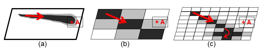
Figure 3Schematic comparison of surface concentration contours and model grid-cell values of a transported pollutant plume from a large stack (termed a “point” source). Wind direction shown by red arrows. Monitoring station location marked by “+A”. (a) Actual plume. (b) Coarse grid-cell size air-quality model prediction. (c) Fine grid-cell size air-quality model prediction. Note the change in wind direction between observations (a) and simulations (b, c) associated with errors in the forecast of the synoptic wind.
In addition to the standard analysis, we perform additional analyses that examine the model's ability to resolve plumes in the vicinity of the observation station, in order to attempt to evaluate the potential for higher-resolution simulations to provide benefits which may be masked by synoptic-scale forcing errors. This strategy is illustrated in Fig. 4.
Figure 4a shows an observation station enclosing the nine nearest-neighbour model grid cells for a 2.5 km grid-cell size, while Fig. 4b shows the corresponding 1 km grid-cell size map, with the 9 nearest-neighbour model grid cells shown in light grey and the 49 nearest grid cells shown in the region enclosed in dark grey. Figure 4a encloses a region of 56.25 km2 (7.5 km × 7.5 km), while the light grey region in Fig. 4b encloses 9 km2, and the darker grey region encloses 49 km2.
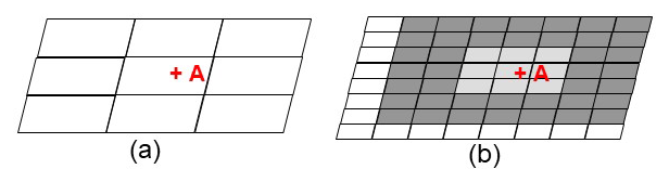
Figure 4Scale diagram of the same region in (a) a 2.5 km grid-cell size simulation and (b) a 1 km grid-cell size simulation. Region enclosed by light grey (dark grey) shading in (b) represents the nearest 9 (49) 1 km grid points surrounding the observation location “A”.
As noted above, in a formal mathematical sense, the smallest region resolvable by an Eulerian grid model is twice the size of the model grid-cell size (relating to the Nyquist frequency of the model); hence the smallest resolvable feature spans two model grid cells in each direction. However, in a practical sense, a total of nine grid cells centered on the observation station must be used to allow a boundary of two grid cells in any direction. Sampling any or all of the nine grid cells in Fig. 4a may thus be said to be representative of the model's ability to simulate events occurring at discrete location “+A”. The closest corresponding sampling region available to the 1 km model (Fig. 4b) is shown in dark grey. The light grey region of Fig. 4b represents the closest 1 km grid-cell size region that corresponds to the single 2.5 km grid cell in which the observation station is located in Fig. 4a. We attempt to ascertain model performance in these approximately equivalent regions around each observation station, in the analysis that follows.
Our approach follows two steps:
-
From the 2.5 km simulation, in addition to the predicted model value at the grid cell containing the observation location, we determine the model grid-cell value in the nine grid cells surrounding the observation station location which has the closest value to that observed at the station. This represents the model's “best estimate” of the value at the observation station location itself and represents the model's ability to resolve features at 2.5 km grid-cell size.
-
From the 1 km simulation, in addition to the model value at the grid-cell location, we select the closest value to the observation value from
- a.
the nearest nine grid cells to the observation station location, and
- b.
the nearest 49 grid cells to the observation station location.
The former represents the model's “best estimate” of the value at the observation station location itself, while the latter represents the 1 km model's best estimate in the closest equivalent region to the limiting resolution of the 2.5 km model.
- a.
Comparing the resulting statistical measures of each of these selected values with observations, in addition to the standard analysis, thus evaluates the model's best attempt to resolve features for the specified grid-cell size and allows cross-comparison of model performance within nearly equivalent areas. Cross-comparing the statistical values for the different regions described above shows the model's ability to resolve features such as plumes from the standpoint of the region represented at the different grid-cell sizes. If synoptic-scale transport direction errors create situations similar to that depicted in Fig. 3a, a standard comparison of error would be expected to show little benefit to higher resolution. However, the “best model estimate” comparisons would capture the ability of the higher-resolution model to more accurately simulate the magnitude of the plume, if not its spatial location. Each of these selection procedures will be employed in the surface concentration comparisons which follow.
We evaluate our model simulations against observations made at surface monitoring networks in the vicinity of the Athabasca oil sands, and aboard an instrumented aircraft, the National Research Council of Canada Convair. For the surface monitoring data, hourly time series of model output were matched to station time series using the different strategies described above. For the aircraft observations, we extract model values through temporal and spatial interpolation to the aircraft's position during the flights and only perform the standard analysis, as well as examining the behaviour of the two simulations along cross sections corresponding to the flight paths.
Our statistical metrics for evaluation are common to many other air-quality applications and were computed using the “modstat” function from the OpenAir R package (Carslaw and Ropkins, 2012). Further discussion of different metrics for model evaluation may also be found in Yu et al. (2006). The statistics calculated here include mean bias (MB; perfect score: zero), mean absolute gross error (MGE; perfect score: zero), normalized mean bias (NMB; perfect score: zero), normalized mean gross error (NMGE: perfect score: zero), root mean squared error (RMSE; perfect score: zero), correlation coefficient (r, perfect score: unity), coefficient of efficiency (COE: a perfect score is unity, a zero or negative score means the model is equivalent or less predictive, respectively, than the mean of the observations), and the index of agreement (IoA; perfect agreement is unity, and −1 indicates no agreement or little variability).
3.1 Model-to-model comparisons and averages
We begin a comparison of 2.5 and 1 km grid-cell size for specific events, and for averages across the 1 km domain, in order to provide a qualitative comparison of the differences in simulations for the two simulations and then continue with the quantitative comparison. Figure 5 compares OS2.5km (left column) and OS1km (right column) simulation results for a cross section located 0.2 km from a major SO2 emissions source at 00:00, 12:00, and 24:00 UT into a given simulation day.
The model results are identical at hour 0 due to both the OS2.5 and OS1km models being initialized from the OS10 km data at this time (small differences between Fig. 5a and b are due to slight mismatches in the cross section locations). Subsequent cross sections show the OS1km model is capable of resolving both higher absolute mixing ratio values, and sharper gradients, within 12 h of simulation time (Fig. 5c, d). Multiple plumes are resolved by 12 h of simulation time in the 1 km grid-cell size simulation, along with markedly different plume heights, plume structure, and an increase of a factor of 2 in the magnitude of plume mixing ratios relative to the lower grid-cell size simulation, and these differences persist into the 24th simulation hour (Fig. 5e, f). Mixing ratio differences of these magnitudes are to be expected given the increase in resolution, but Fig. 5 shows that other important aspects of the predicted plumes have changed. The plume heights are a function of predicted local stability conditions in the grid square containing the source, and the variation shown here represents a substantial change in the predicted local stability for the origin sources of these plumes, resulting from the change in model horizontal grid-cell size.

Figure 5Comparison of simulated SO2 plume mixing ratios (ppbv) located 0.2 km from a major point source, for OS2.5km simulations (a, c, e) and OS1km simulations (b, d, f), at 0 (a, b), 12 (c, d), and 24 h (e, f) into a 24 h simulation.
Figure 6 compares the maximum surface SO2 during the entire period for each simulation, as well as the difference in maximum SO2 between the simulations, along with a scatter plot of OS2.5 vs. OS1km simulation results. In the latter two panels, OS2.5km values were assigned to the corresponding OS1km grid-cell locations using the nearest-neighbour approach.
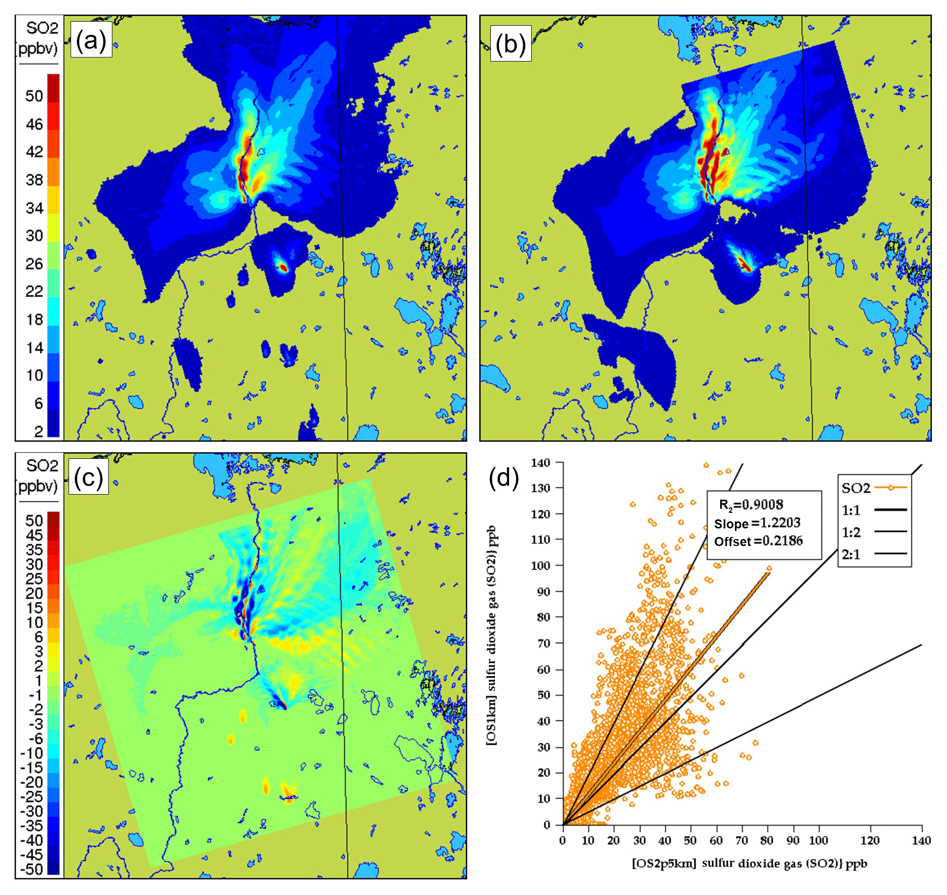
Figure 6Comparison of total-simulation maximum surface SO2 mixing ratios (ppbv) at (a) 2.5 km and (b) 1 km grid-cell size (ppbv). (c) Difference (2.5−1 km). (d) Scatter plot of 2.5 km (x axis) versus 1 km (y axis) total simulation average grid-cell surface SO2 mixing ratios.
The maximum surface concentrations tend to show more elongated structures at the smaller grid-cell size, comparing Fig. 6a and b, particularly for plumes in the western (left) half of the OS1km domain. The difference plot (Fig. 6c) shows that local maximum concentration differences of up to −45 ppbv occur, due to changes in the placement and maximum concentration of high-concentration plumes. The scatter plot of Fig. 6d shows that OS1km model has a demonstrated ability to achieve higher concentrations than the OS2.5km model, with a slope of 1.22, and a noticeable clustering of values along the 1:2 line. While these results are not unexpected since approximately 95 % of the SO2 emissions in the domain originate in large stack, or point, sources, and hence initial concentrations at source would be expected to 6.25× higher in the OS1km simulation, they also suggest that a substantial improvement in the OS1km model's ability to capture SO2 concentrations should be possible. That is, the results of the two models are substantially different, and given the reduction in numerical error expected with employing a smaller grid-cell size, the latter might be expected to outperform a larger grid-cell size model. However, as we shall demonstrate in the next section, plume placement errors such as those depicted in Fig. 3 play a substantial role in model performance as grid-cell size decreases.
3.2 Quantitative comparisons
3.2.1 Surface observation comparison
The locations of the local network of 10 surface monitoring stations located near the sources of emissions in the region (oil sands facilities) are shown in Fig. 7. As noted in Sect. 2.4, we carry out several analyses:
-
The standard evaluation. The model values are extracted from the model grid cells containing the observation stations, at both grid-cell sizes.
-
Equal areas of representativeness, 1 and 2.5 km grid-cell sizes. The nearest nine OS1km grid cells are compared to the OS2.5km single cell evaluation in two ways:
- a.
averaging of the OS1km results across the nine grid cells prior to evaluation (to determine whether the mean value is better represented by the smaller grid-cell size, similar to the approach taken in Kang et al., 2007);
- b.
selection of the best of the nine grid cells (closest to the observation value), to determine the extent to which the OS1km model is capable of better representing the concentrations somewhere within the corresponding OS2.5km model grid cell, if not at the OS1km cell closest to the observation location – higher scores for the 1 km grid-cell size simulation in this case would indicate that while errors in plume positioning (for example due to errors in the synoptic-scale flow) negate some of the advantages of the OS1km simulation, the plume may be better represented by the OS1km simulation within the 2.5 km grid cell's area.
- a.
-
Equal areas of representativeness and equal regions of variability. The nearest 9 2.5 km cells are compared to the nearest 49 1 km cells. Here we make the assumption that the 2.5 km grid-cell size model's ability to resolve features is limited to the surrounding three grid cells in each horizontal dimension and make use of the closest-in-size block of corresponding 1 km cells (a 7×7 grid centered on the cell containing the observation point). In both cases, the model value closest to the observations is chosen prior to evaluation.
While evaluations (Figs. 2b and 3) deliberately select the “best” value, they also provide a quantitative estimate of the extent to which each model is capable of achieving the correct answer within roughly equal representative areas centered on the observation station locations. These comparisons are intended to evaluate
- a.
the extent to which the 1 km grid-cell size is capable of improving simulation results despite, for example, the larger-scale flow resulting in errors in the plume placement, and
- b.
whether the 1 km grid-cell size model is capable of outperforming the 2.5 km grid-cell size model over equivalent regions.
In the last test, we place both models on an equal footing with regards to the region being represented, as well as with regards to allowing cell-to-cell variability and the selection of a closest match to observations.
Our evaluation is presented as tables of statistical metrics. The comparisons employing the nearest-neighbour approach are described with a “Bn” superscript suffix, denoting that the “best” sample within a square centered on the observation point containing a total of n grid cells (e.g. the OS1kmB9 label denotes a comparison between observed data and the simulation grid cell within a 3×3 grid-cell square centered about the observation point). Similarly, an An superscript describes a comparison between the observations and the average of the n square of grid cells centered on the observation point.
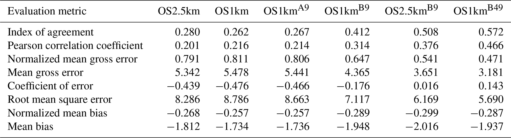
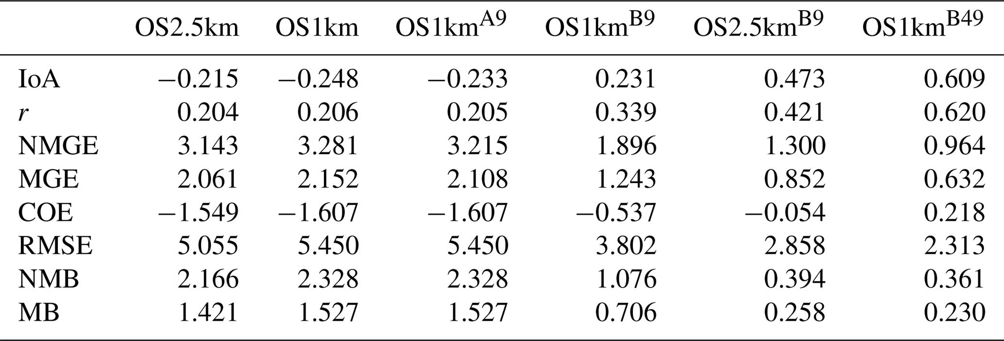
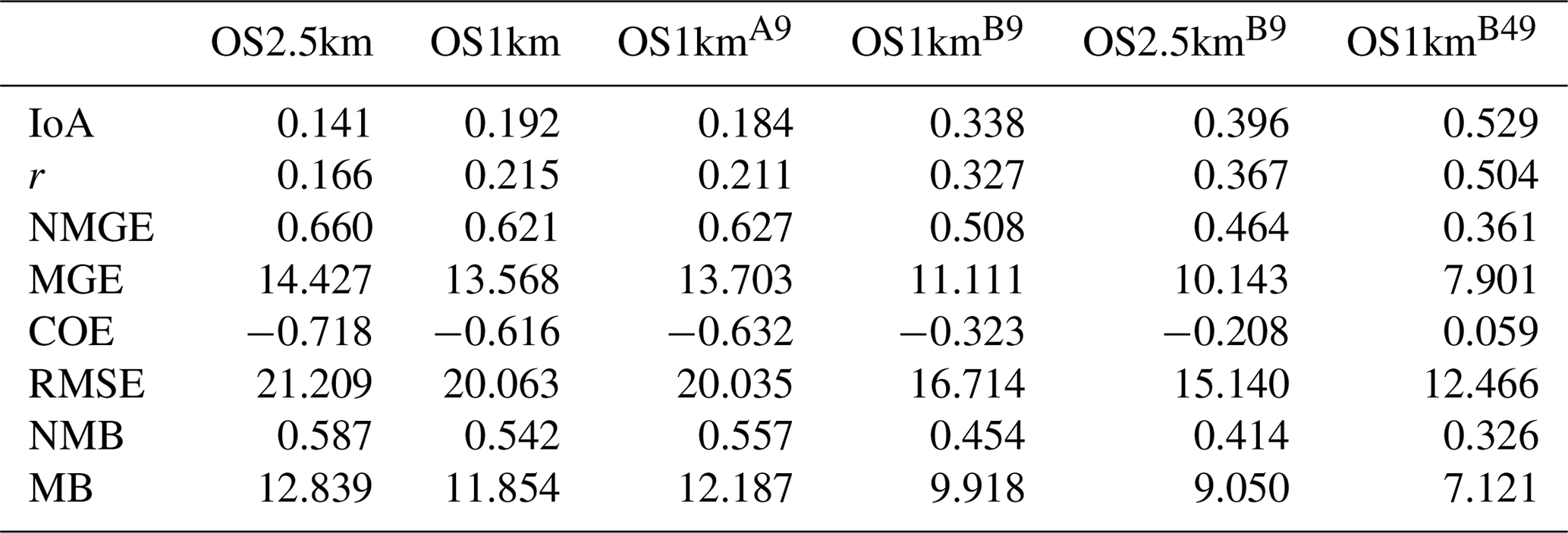
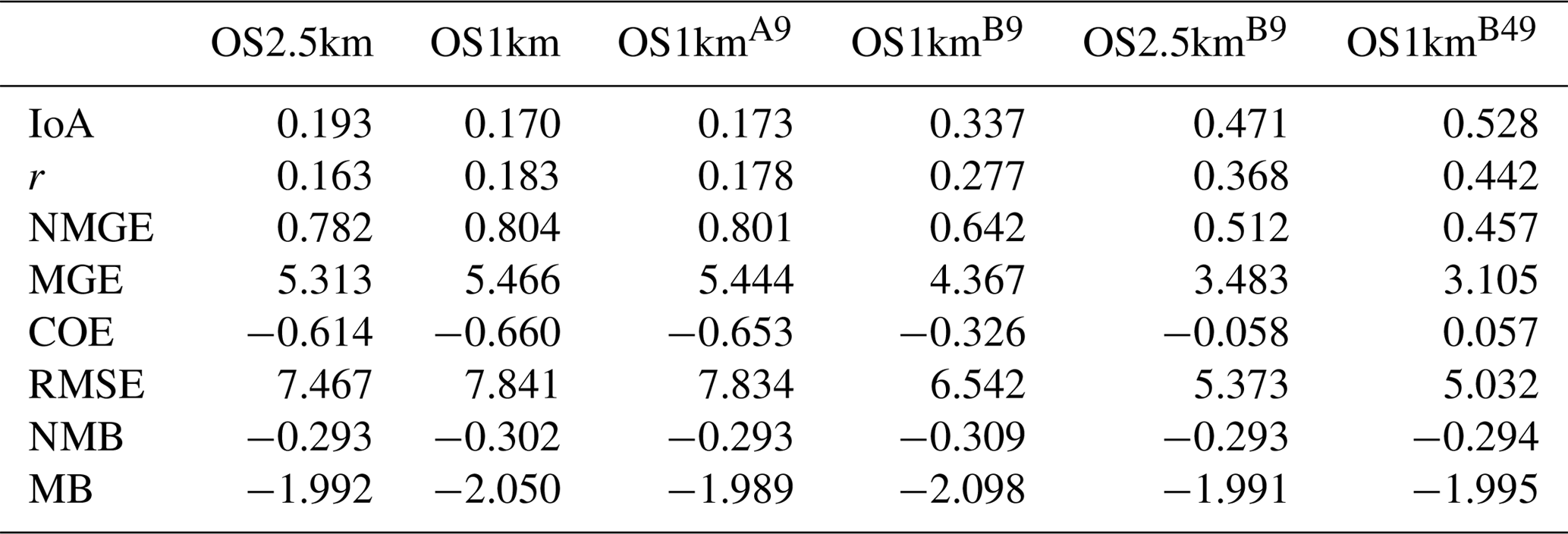
Comparisons to surface concentrations were performed using publicly available data collected by the Wood Buffalo Environmental Association (WBEA), which operates the air-quality monitoring network residing within the OS1km domain. The monitoring station locations are shown in Fig. 7. The statistical performance of the models, calculated using the procedure outlined above, are given in Tables 2 through 5, for SO2, NOx, O3, and PM2.5, respectively.
In the standard model grid cell to observation measurement comparison for SO2 and NOx (first two columns, Tables 2 and 3), the OS1km simulation had worse scores for all the metrics considered here. For O3, the OS1km model had the better score for the correlation coefficient and root mean square error, and worse scores for all remaining model evaluation metrics. For PM2.5, the OS1km model showed a better performance for the correlation coefficient and biases, while the OS2.5km model outperforms the OS1km model for all other metrics examined here. Based on a standard analysis, the OS1km model thus performs poorly compared to the OS2.5km model; the expected advantages associated with reduced numerical error in transport at smaller grid-cell sizes are being offset by other factors controlling the net model error.
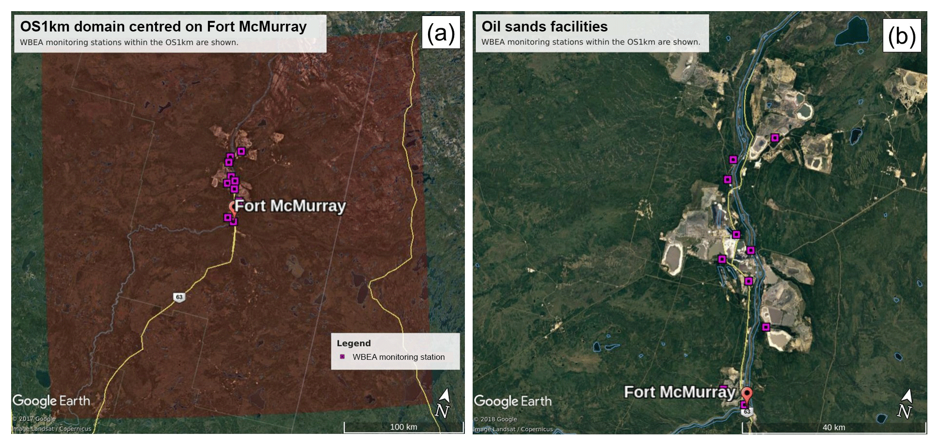
Figure 7Illustration of the OS1km domain, with observation station locations. (a) Entire domain. (b) Close-up view of station locations. Monitoring stations are shown as purple outline squares in both images. Light grey regions in the background satellite image (b) are oil sands open-pit mining operations.
When the standard evaluation is compared to the average of the nearest nine 1 km simulation grid cells surrounding the observation point (third column of the tables), an intermediate result appears. For SO2 (Table 2) the nine-cell OS1km average has the best performance for correlation coefficient – indicating a better time distribution of events may be achieved by a nine-cell average at 1 km grid-cell size. The other metrics for the A9 simulation are intermediate between the two standard evaluations for each simulation, indicating that some of the performance loss resulting from the use of 1 km grid-cell size is reduced through averaging results to approximately the same size regions as the OS2.5km grid-cell size. The latter result holds for all metrics for NOx (including R, see Table 3). For ozone (Table 4), averaging the nine nearest OS1km grid cells prior to measurement gives the best performance for R and RMSE, and worse performance for the other metrics. For PM2.5 (Table 5), all metrics for the OS1km nine grid-cell average aside from the bias fall mid-way between the two standard methodology evaluations. Averaging the smaller grid-cell size model results thus shows a marginal improvement, depending on the species, but overall does not compensate for the decrease in performance resulting from going to the smaller grid-cell size.
We next ask the question, “does a more accurate simulation value exist within the same region of the 1 km model as is encompassed by a 2.5 km grid cell?” (fourth column of Tables 2–5), by selecting the model value in the nearest nine 1 km grid cells with the closest match to observations and comparing to the corresponding single 2.5 km grid cell. A dramatic improvement in the relative OS1km performance metric scores can be seen. For each of Tables 2 through 5, this “best of nine” 1 km comparison outperforms the previous 3 comparisons (columns 1 through 3), for all metrics. These improvements are sometimes dramatic (e.g. a doubling of correlation coefficient along with a reduction in mean bias by a factor of 3, a reduction of NOx mean bias values by a factor of 3, a shift of coefficient of error from negative to positive values for O3, and a reduction in the coefficient of error for PM2.5 by a factor of 2.5 compared to the nearest competing value from the previous evaluations. The coefficients of efficiency for SO2 and O3 make the transition from negative to positive values when the “best-of-nine” methodology is used, indicating that the model is able to predict the observations better than the observed mean, somewhere within an equivalent area. This evaluation suggests that the OS1km model does contain a better result within the same approximate region encompassed by a 2.5 km grid cell. However, the location of that better result may be subject to positioning error, such as those described in Fig. 3.
A valid argument could be made that the methodology employed in this fourth evaluation is subject to selection bias, in that the selection of a best value in the case of the nearest nine 1 km simulation places that model simulation at an advantage relative to the 2.5 km model. To address this last issue, the final two additional methodologies for evaluation were employed, still maintaining the same approximate area of representativeness for a grid cell, namely choosing the best value out of the nearest 9 2.5 km grid cells (the limiting resolution of this model simulation), and the best value out of the nearest 49 1 km grid cells (fifth and sixth columns, respectively, of Tables 2 through 5). That is, we attempt to place the two models on an equal basis with regards to selection bias within a given region containing an observation station.
Two important results can be seen from this final evaluation. First, as was the case for the “best of 9” for the OS1km simulation compared to the standard OS1km evaluation, the best of 9 for the OS2.5km simulation has a considerably better performance than the standard OS2.5km evaluation (compare fifth and first columns, Tables 2 through 5). That is, the OS2.5km model may also be subject to location errors in transported species representation which influence model performance. However, when performance within the 56.25 km2 area surrounding each measurement point in the OS2.5km best of 9 evaluation is compared to the 49 km2 area surrounding the measurement points in the OS1km best of 49 simulation (i.e. compare columns five and six in Tables 2 through 5), it can be seen that the OS1km model outperforms the OS2.5km model for all metrics for O3 and PM2.5, and all metrics aside from bias for SO2 and NOx. That is, despite the OS1km model having a slight disadvantage in the relative size of the representative area containing the measurement station location, and both models being allowed a similar selection strategy, the OS1km model is capable of generating values closer to the observations than the OS2.5km model within an equivalent sub-region, across most of the metrics and chemical species considered here.
This final result is strongly suggestive of the presence of issues such as those illustrated in Fig. 3. These may include errors in the larger-scale synoptic wind flow, combined with the reduced size of plumes as grid-cell size is reduced, leading to more “misses” than “hits” for a given recorded event at a measurement station compared to the coarse grid-cell size model. There may be multiple additional causes for such errors (examples include poor observation density in the region for model initialization, underlying lower-resolution boundary condition fields such as topography not improving with the reduction in grid-cell size, inaccuracies in land use fields used in meteorological modelling due to rapid development, and errors in other aspects of the reaction transport modelling system aside from horizontal resolution). The expected advantages of the small grid-cell size, such as better representation of the concentrations of species within plumes and hence better representation of their reactive chemistry (see for example Lonsdale et al., 2012), may be lost in a standard performance analysis due to these other issues.
Our analysis suggests that a practical limit in the benefits of increasing model accuracy may be reached when resolution exceeds some threshold, as a result of other errors inherent in the modelling system. However, the analysis also suggests that if these non-resolution-related errors are corrected, the benefits of adopting a smaller grid-cell size may be substantial. For example, meteorological data assimilation employing a dense monitoring network for a specific area of interest would be expected to show a greater impact for smaller rather than larger grid-cell sizes, due to the greater ability of the former to take advantage of the observation density in correcting the initial meteorological state. We note that recent work applying land use data assimilation (Carrera et al., 2015) to regional 2.5 km grid-cell size weather simulations (Milbrandt et al., 2016) have suggested that such data assimilation may indeed improve forecast skill at the very local scale.
Table 2Surface SO2 observations to model comparison for entire simulation period (ppbv, 5466 model–observation pairs).
Table 3Surface NOx observations to model comparison for entire simulation period (ppbv, 3257 model–observation pairs).

Table 4Surface O3 observations to model comparison for entire simulation period (ppbv, 2189 model–observation pairs).
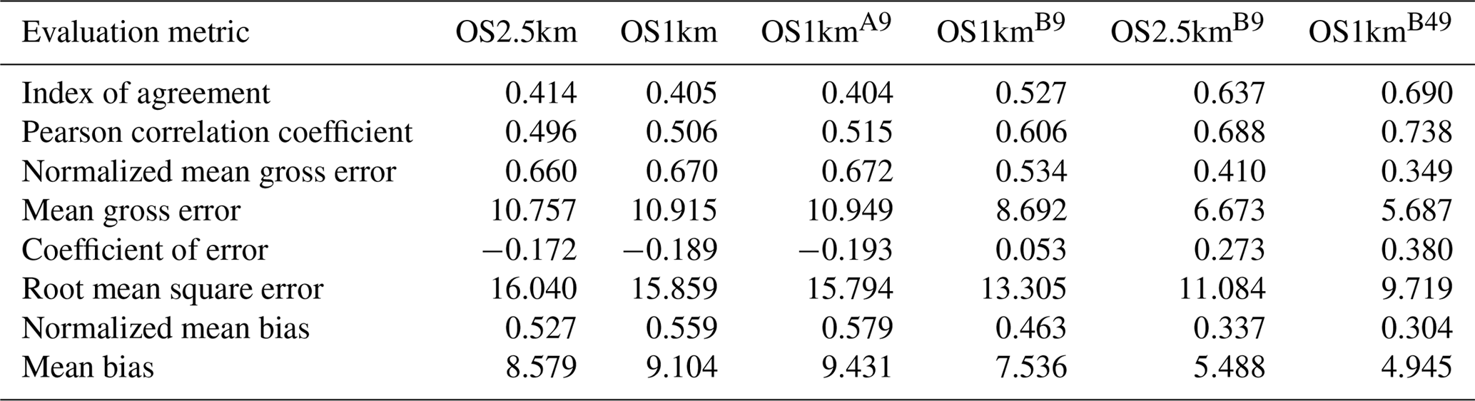
Table 5Surface PM2.5 observations to model comparison for entire simulation period (µg m−3, 3377 model–observation pairs).
The surface observation data were also analyzed by the time of day, with both observations and simulations split into daytime (09:00 to 18:00 LT) and nighttime (19:00 to 08:00 LT) data pairs (Appendix A, Tables A1 through A8; Carslaw and Ropkins, 2012). Within each of these diurnally segregated time periods, the broad aspects of the comparison were the same as for the “all data” Tables 2 to 5 above: the OS1km simulations tended to have reduced performance in a standard analysis, averaging improved but did not completely ameliorate the performance of the OS1km simulation, a methodology employing the best of nine OS1km grid cells had superior performance to the two standard comparisons, and comparison of the “best of” methodologies for equal areas showed better performance for the OS1km compared to the OS2.5km simulation. We also noted substantial differences in the day and night performance of both models across the methodologies. For example, daytime SO2 and NOx performance within a given model and comparison methodology was usually better than nighttime performance for IOA, R, NMGE, COE, and NMB, while worse for RMSE, while nighttime O3 performance was better for IOA, r, NMGE, and COE. Daytime PM2.5 performance was better than nighttime for IOA, r, COE, and NMB. The study area is located in a broad river valley with frequent slope-defined anabatic/akatabic and drainage flow events. These often have a diurnal nature, and may explain part of the day–night differences. Example sources of these differences may include the relative ability of the driving meteorological model to capture daytime versus nighttime mixed layer turbulence and the planetary boundary layer height.
3.2.2 Comparisons to aircraft observations
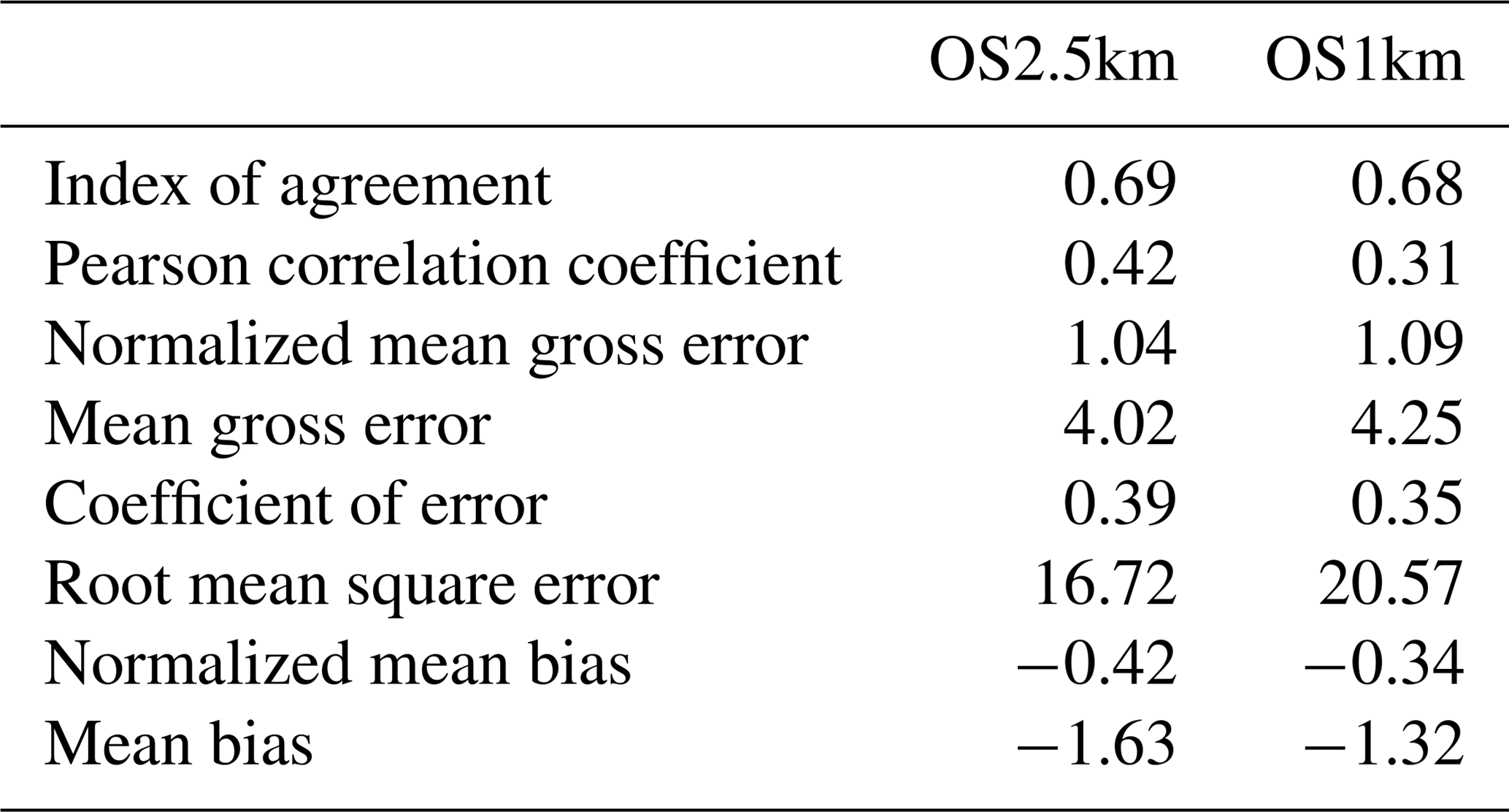
A total of 22 aircraft observation flights were carried out during the study simulation period – here we present statistical comparisons using the standard approach only (model grid cell containing the observation point to observation data at the aircraft location). Model values were linearly interpolated in time and space to the aircraft observation locations and times (aircraft observations were on a 10 s interval.) We begin with a composite comparison across all observation times, in Table 6.

The results are in general similar to the surface analysis, in that the OS1km simulation tended to have worse performance than the OS2.5km simulation (exceptions being the biases for both SO2 and NO2, and the slightly better OS1km correlation coefficient for SO2). One striking difference between the first two columns of Tables 2 and 3, compared to Table 6, is the magnitude of the differences between the simulations. Aloft (Table 6), the differences in performance metric magnitudes between OS2.5 and OS1km simulations are much smaller than at the surface (Tables 3 and 4). The biases are negative aloft and positive at the surface, indicating that both models may be lofting plumes to insufficient distances; one of the possible (non-horizontal grid-cell-size-dependent) causes of model error may be in the extent of vertical transport. This possibility is examined in more detail in Akingunola et al. (2018) and Gordon et al. (2018). An example of this behaviour is shown in Fig. 8; both plumes fumigate to the surface, while the observed plume resides largely aloft. The OS1km model captures the higher concentrations to a better degree, but the impact of excessive fumigation more than offsets this improvement, as is shown by the performance evaluation of Table 7, where both models have negative biases aloft. In this particular case, the tendency of the model to overestimate the extent of fumigation has a bigger impact on performance than grid-cell size. Garcia-Menendez et al. (2014) have noted similar results for forest fire plume prediction.
Figure 8a and c provide a further example of the kind of situation referenced in Fig. 3; surface monitoring station locations are depicted as grey circles, one of which is identified with a pink arrow. This station lies within the plume at 2.5 km resolution (Fig. 8a), and outside of the plume at 1 km resolution (Fig. 8c). While the plume direction is the same at both scales, that is, the large-scale wind field controls the positioning of the plume axis, the smaller grid-cell size simulation places a stronger constraint on the accuracy of the wind field. For example, if the simulated large-scale flow direction was inaccurately predicted by only a few degrees, the plume would not appear in the 1 km simulation time series at this location but would register as present in the 2.5 km simulation. Nevertheless, the plume maximum concentration is better captured by the smaller grid-cell size simulation (compare maximum values in observed aircraft SO2; Fig. 8b, d). The higher-resolution simulation may thus more accurately simulate the plume maximum concentration – but not its placement in space, as was hypothesized in Fig. 3.
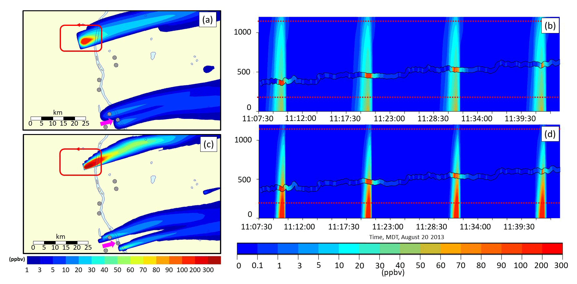
Figure 8Comparison between OS2.5km (a, b) and OS1km (c, d) simulations for SO2 relative to aircraft observations (ppbv). (a, c) Simulated surface concentrations of SO2, with the flight track shown as a red line. Grey circles: surface monitoring station locations; pink arrow indicates a station located inside a plume at 2.5 km resolution (a), and outside the plume at 1 km resolution (c). (b, d) Portion of the simulated concentration profiles along the flight path as a function of time. Successive intersections of the flight path with the plume appear as background colour contours; observed SO2 aboard the aircraft is shown between the two black lines. Vertical axis is elevation above the ground; the aircraft elevation is increasing with successive passes around the facility. Dotted lines show the upper and lower vertical extent of the observed plume; note that for both model simulations, the plume erroneously fumigates the surface.
Table 7Standard performance evaluation of Flight 8 for SO2 (ppbv, 1261 model–observation pairs).
Meanwhile other flights show a clear advantage of the OS1km model. One example is given by the NO2 performance evaluation of Table 8 and depicted in Fig. 9, for Flight 17 (a similar flight plan carried out around the same facility as Flight 8). While the correlation coefficient degraded slightly in the OS1km resolution simulation, all other performance measures were improved with the decrease in grid-cell size. Two time-versus-height-profile cross sections for Flight 17 are shown in Fig. 9. In Fig. 9a and b, the OS2.5km and OS1km simulations, respectively, are compared for the portion of the overall flight track circling the given facility. This comparison clearly shows that the OS1km model does a better job of capturing the width of the high-concentration region of the plume – however, the location of the model plume lags the observations. During this portion of the flight alone, the OS2.5km model statistics, particularly the correlation coefficient, outperform the OS1km model, due to this issue of plume location mismatching. Figure 9a and b may be compared to Fig. 3a and b – the same situation is depicted in both figures. Figure 9c and d show the OS2.5km simulation (Fig. 10c) and OS1km simulation results in another portion of the flight – here the OS1km performance for most statistics was better than the OS2.5km model performance. The OS1km model (Fig. 9d) captures the existence of a lower-concentration layer aloft in the right-hand side of the cross section, and the existence of low-concentration intervening layers, as well as the overall lower concentrations of SO2, while the OS2.5km model does not resolve these fine-scale and lower-concentration features. We note here that IoA, COE, and the other error measures capture the visual impression that the OS1km model outperforms the OS2.5km model for this flight, while the correlation coefficient is highly dependent on the placement of the plume maximum in the upper two panels.
These and the snap-shot comparisons described in Sect. 3.1 show that the higher-resolution model is having a significant impact on predictions – however, other aspects of the overall model performance are preventing the potential benefits of higher resolution from influencing the standard performance evaluation.
Table 8Standard performance evaluation of Flight 17 for NO2 (ppbv, 1174 model–observation pairs).
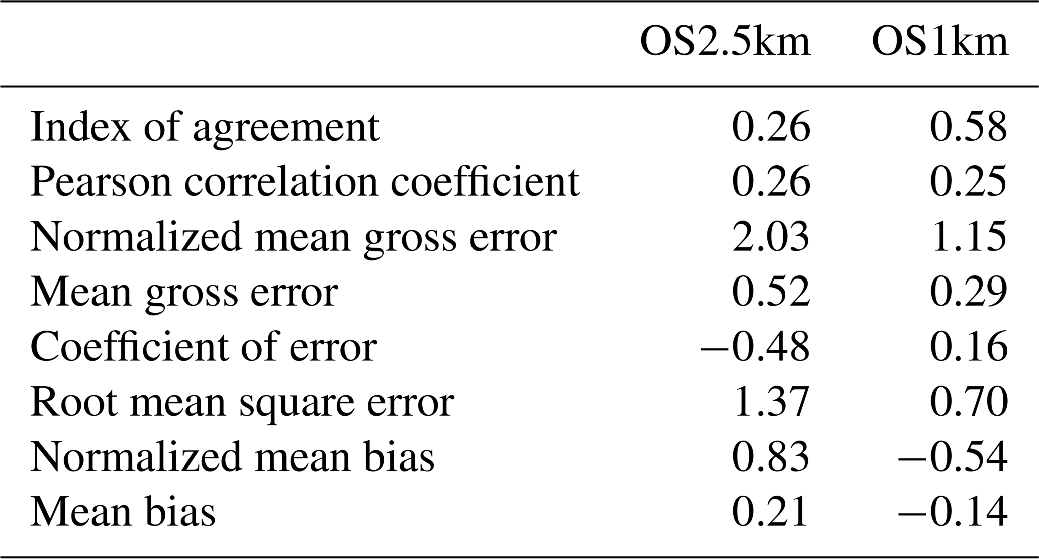
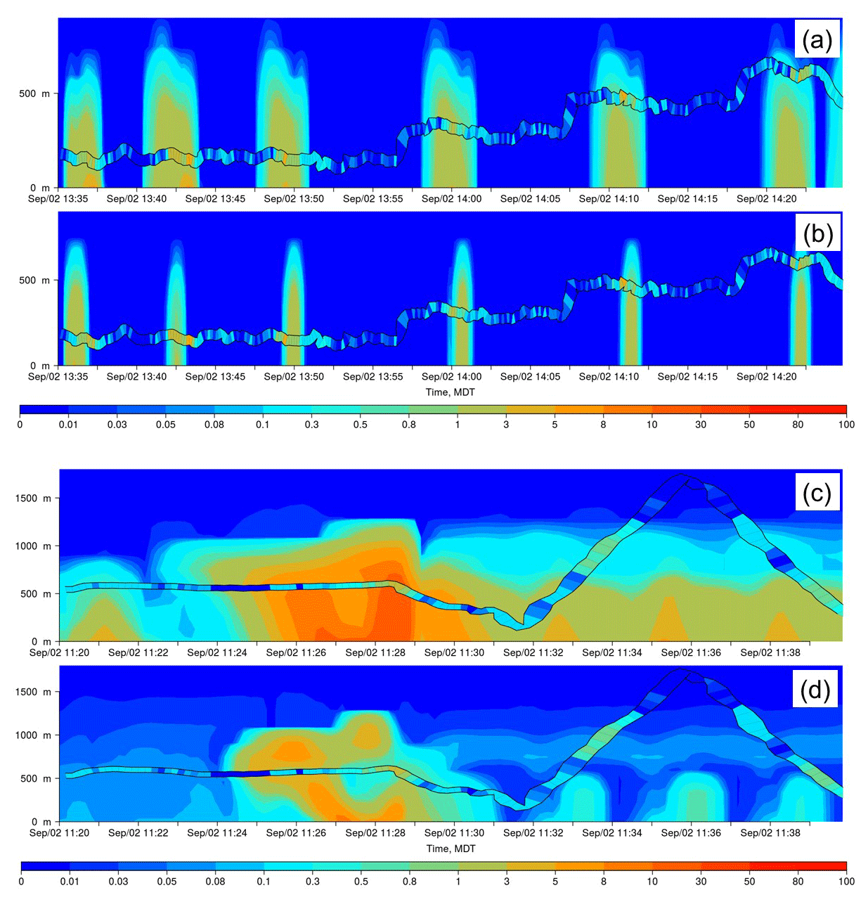
Figure 9Flight 17 comparison for NO2 (ppbv) for portions of the net flight track circling the CNRL facility for OS2.5km (a) and OS1km (b) simulations, and for a later section of the same flight path for the OS2.5km (c) and OS1km (d) simulations.
A key result of our current work is that 1 km grid-cell size simulations resulted in improved prediction of plume concentration maxima relative to 2.5 km grid-cell size simulations, despite having no improvement using standard scoring methodologies. We also have described a scoring approach wherein these potential advantages of higher resolution may be quantified. We believe that flow field effects such as those described in Fig. 3 are a general result of increasing grid resolution, but note important caveats, which include the following:
-
The availability of meteorological observation and high-resolution emissions data to provide model driving information, and the resolution and proximity of this information to the simulation location. Both will influence the relative importance of grid-cell size on model results. If this information is available in a higher resolution than the lower of two grid-cell size simulations being compared, and/or is used via data assimilation to improve model initial meteorological conditions, our expectation is that the smaller grid-cell size model may outscore the larger grid-cell size model, even for more standard metrics.
-
The extent to which local, versus synoptic, weather conditions drive flow in a given region. For example, in the urban heat island meteorological simulations of Leroyer et al. (2014), the accuracy of local flow predictions was shown to be extremely dependent on the representation of the urban heat island, and the accuracy of the latter was critically dependent on the grid-cell size (which in this example went down to 250 m). In this respect, for meteorological conditions wherein local factors can dominate the flow, and where those conditions may be adequately modelled only at very high resolution, we would again expect the smaller grid-cell size simulation to provide better performance, for standard metrics.
-
The results apply as grid-cell size decreases, but are not necessarily true for grid-cell size increases. Conversely, model performance using standard metrics should not be expected to increase with successively larger and larger grid sizes; the accuracy of even the synoptic flow field will not be captured as model resolution decreases.
Given these considerations, we recommend that modellers should attempt successively smaller grid-cell sizes to determine the following: first, the point at which, for their particular system and simulation location, subsequent grid-cell size reductions fail to improve performance, and second, to make use of still higher resolutions for studies wherein the point-to-point comparison is less important, and other factors such as accurately capturing the plume chemistry are more crucial.
Our work suggests the following: decreasing air-quality model horizontal grid-cell size will not necessarily result in improvements to model performance in standard performance evaluations, in which the model values at the grid cells encompassing measurement location stations are used in a pairwise comparison to observations. Other considerations, such as the accuracy of the larger-scale wind direction and speed forecast, and the accuracy of the plume rise parameterization used within the model may play a greater role in the overall performance of the model, and reduce the benefits of the smaller grid-cell size. In the context of a standard model performance evaluation, there may be fixed limits to the benefits of decreasing model grid-cell size.
Despite this difficulty, our results also show that the use of smaller grid-cell sizes have some potential benefits, in that these models do a better job of resolving specific air pollution features, like high-concentration maxima within plumes. Both coarse and fine grid-cell size plumes may be misplaced in both time and space, with the net result that the latter model has a worse performance in a standard comparison, but is nevertheless more likely to capture the correct in-plume concentrations, and hence the chemistry, of the actual plume, in the neighbourhood of the observation location. When the evaluation is broadened to find the closest fit to observations in the vicinity of the observation station, with models confined to a similar representative area around the observation station, these potential benefits of the smaller grid-cell size become apparent.
Our results should not be taken as an indication that the standard metrics for model comparison are in some way flawed – they provide the most rigorous method for evaluating the performance of a model at specific monitoring locations and specific times. However, the ancillary performance assessment methodology presented here shows that models with very small grid sizes, which may have standard performance metric scores that have not improved or have even degraded relative to larger grid-cell size models, nevertheless have scientific value, in terms of being better able to capture plume concentrations and hence plume chemistry, if not plume position. The work also suggests that the prediction accuracy of very local transport conditions may be a large factor in preventing the smaller grid-cell size models from achieving improved performance in standard performance analyses.
These findings suggest that at the current state of development, VHR air-quality models are of benefit for the specific purpose of chemical process studies, in which the main aim of the work is to accurately simulate plume chemistry – and in which accurate forecasting of the position of the plume in time and space is a secondary concern. Our work also suggests that efforts to improve other aspects of the overall modelling framework which improve the large-scale flow (for example, the use of data assimilation of local meteorology to improve wind direction predictions) may result in greater benefits as smaller grid-cell sizes are employed.
Surface station air monitoring data used in this study were obtained and are publicly available from the Wood Buffalo Environmental Association (https://wbea.org/network-and-data/monitoring-stations/, last access: 1 April 2019). The 2013 aircraft data used in this study are available from the Oil Sands Monitoring site (http://donnees.ec.gc.ca/data/air/monitor/ambient-air-quality-oil-sands-region/pollutant-transformation-summer-2013-aircraft-intensive-multi-parameters-oil-sands-region/?lang=en, last access: 1 April 2019). GEM-MACH model output data generated for this study are available on email request to Paul A. Makar (paul.makar@canada.ca).
The model output generated from the study requires a large amount of memory space (several gigabytes per day of simulation) in a binary format specific to Environment and Climate Change Canada's modelling systems. The size of the files precludes maintenance on a public site, but conversion to other formats and arrangements for uploading may be made on request to Environment and Climate Change Canada at paul.makar@canada.ca.
Table A1Model comparison statistics.
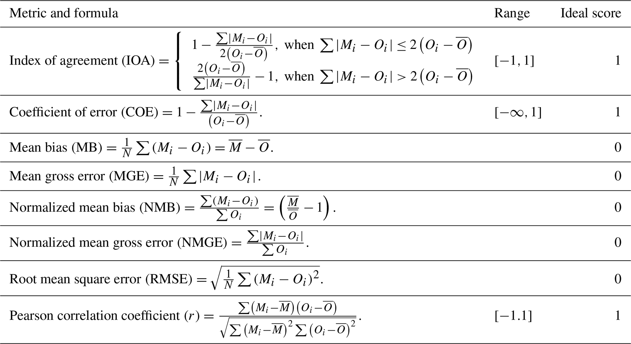
The limits on the summations were removed for brevity; all are from i=1 to N where N is the number of observation–model pairs, Mi is the ith model value, O is the ith observation value, and are the model and observed mean values, respectively.
Table B1Surface SO2 observations to model comparison, daytime (09:00–18:00 LT) (ppbv, 2119 model–observation pairs).
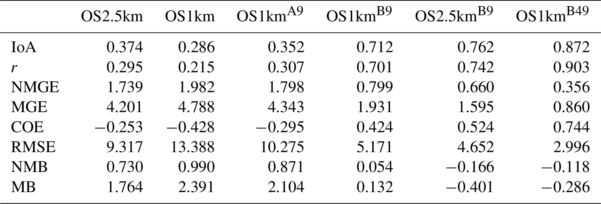
Table B2Surface SO2 observations to model comparison, nighttime (18:00–09:00 LT) (ppbv, 3347 model–observation pairs).
* 3347 samples used.
Table B3Surface NOx observations to model comparison, daytime (09:00–18:00 LT) (ppbv, 1252 model–observation pairs).
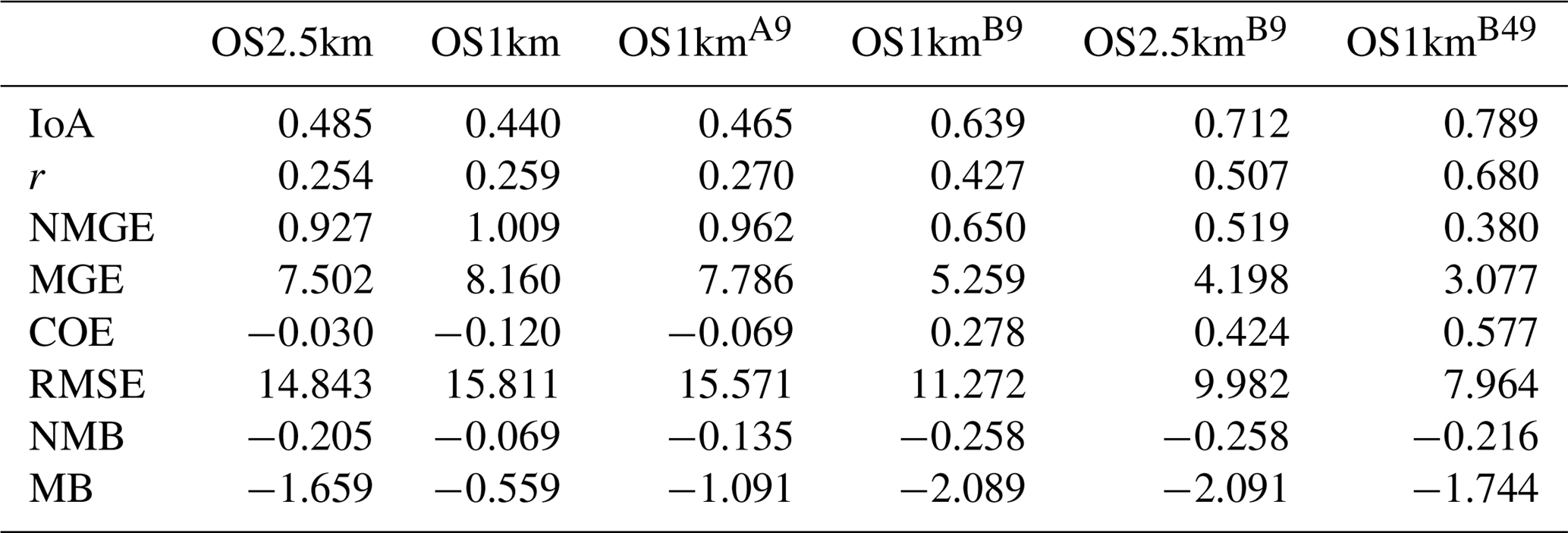
Table B4Surface NOx observations to model comparison, nighttime (18:00–09:00 LT) (ppbv, 1862 model–observation pairs).
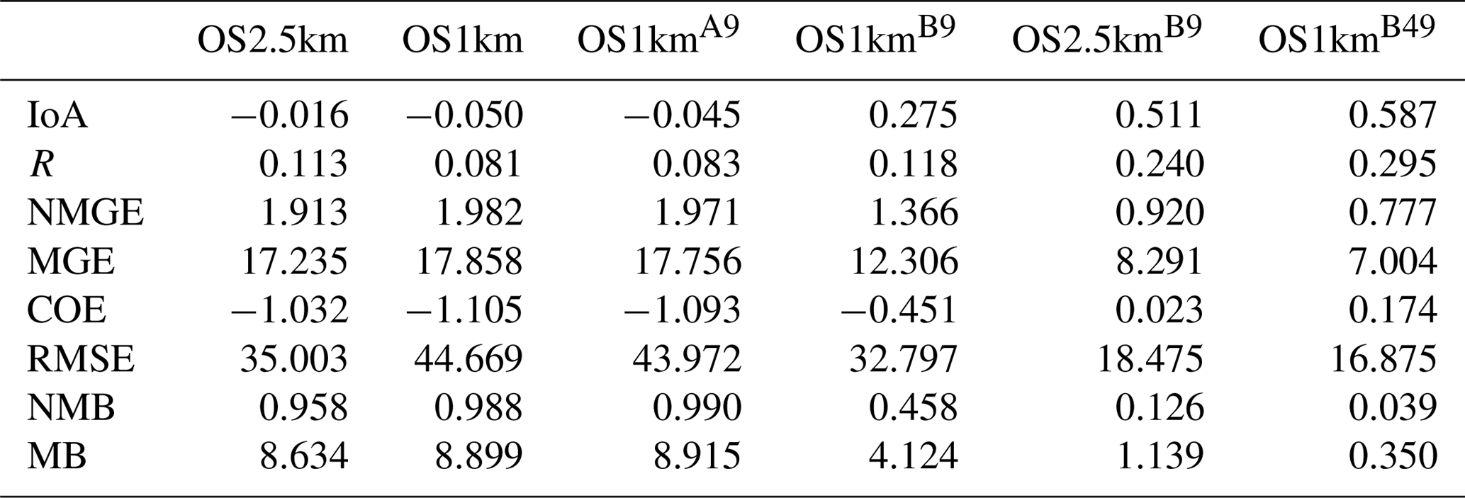
Table B5Surface O3 observations to model comparison, daytime (09:00–18:00 LT) (ppbv, 864 model–observation pairs).
* 864 samples used.
Table B6Surface O3 observations to model comparison, nighttime (18:00–09:00 LT) (ppbv, 1247 model–observation pairs).
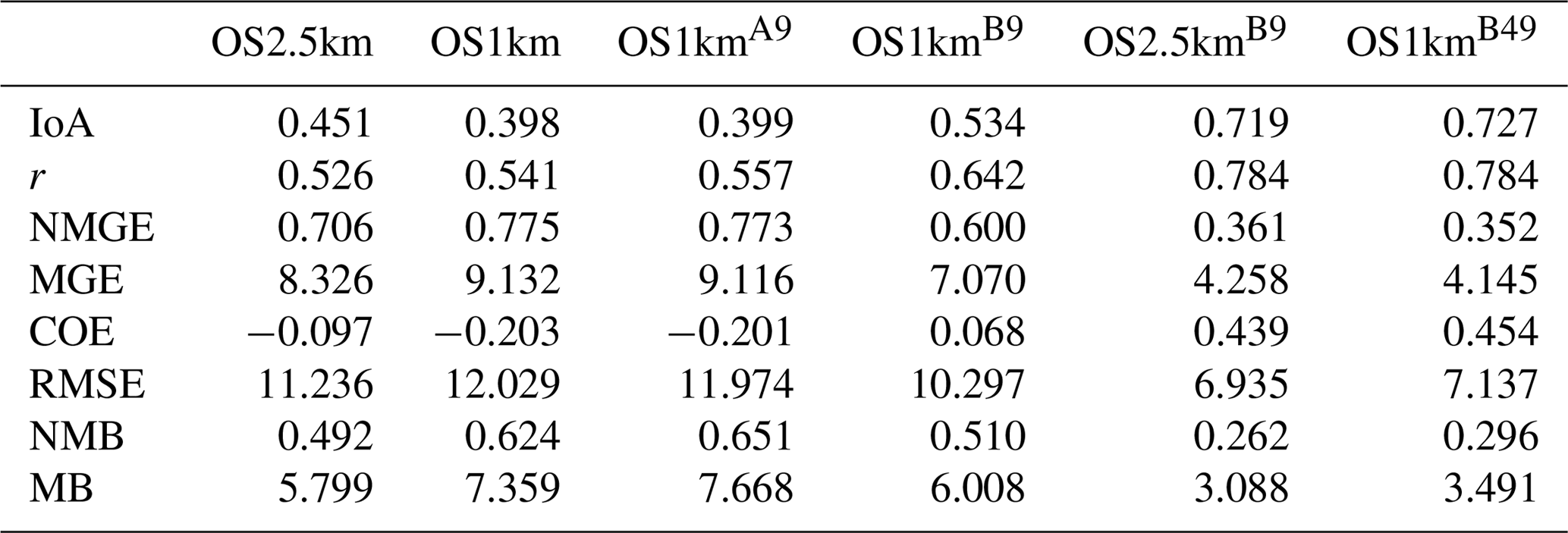
Table B7Surface PM2.5 observations to model comparison, daytime (09:00–18:00 LT) (µg m−3, 1862 model–observation pairs).
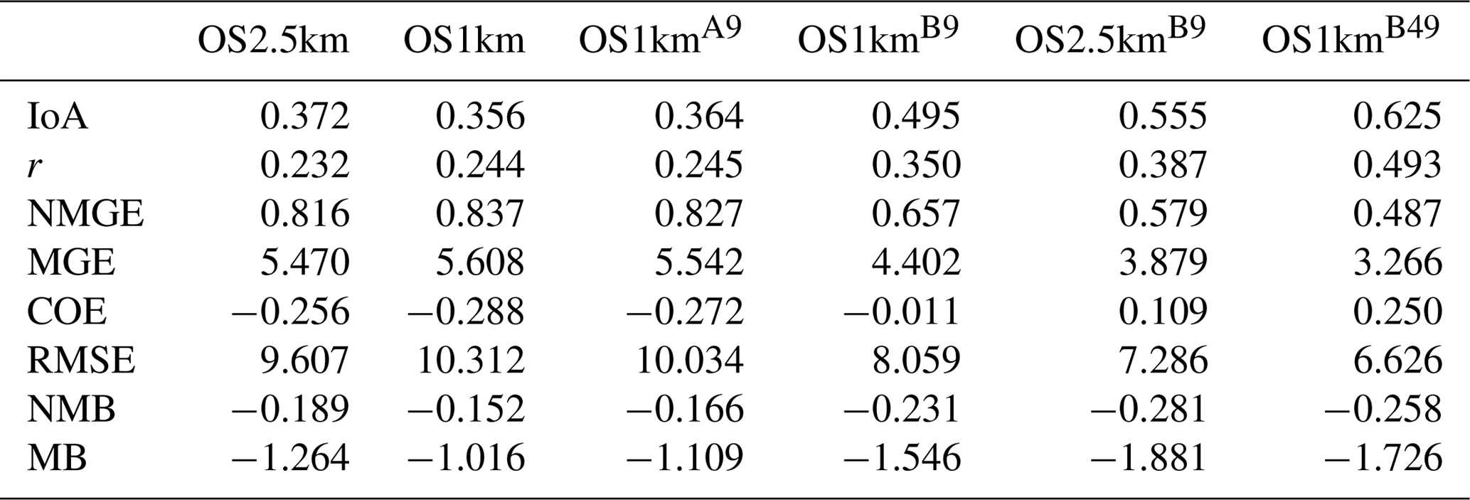
Table B8Surface PM2.5 observations to model comparison, nighttime (18:00–09:00 LT) (µg m−3, 1862 model–observation pairs).
MR conducted computer simulations and analysis and created graphical outputs and the initial manuscript draft. AH supervised MR, provided research advice and infrastructure, contributed to manuscript writing, and provided comments on manuscript drafts. PAM co-supervised MR, provided research advice and infrastructure, contributed to manuscript writing, and was the lead for revisions and responses to referees. AA provided model code assistance and setup, and the scoring package for model–observation comparisons. JZ provided 2.5 and 1 km resolution emissions files. MDM provided 2.5 and 1 km resolution emissions files and commented on manuscript drafts. QZ contributed to the provision of 2.5 and 1 km resolution emissions files.
The authors declare that they have no conflict of interest.
The authors wish to thank the support of Environment and Climate Change Canada (ECCC), under the CCAP program, for supporting this research. The authors also gratefully acknowledge the assistance of Michel Valin and Sylvie Gravel for advice and assistance with the installation of GEM-MACH on the Carleton University workstations during the early stages of this project.
This paper was edited by Jason West and reviewed by two anonymous referees.
Akingunola, A., Makar, P. A., Zhang, J., Darlington, A., Li, S.-M., Gordon, M., Moran, M. D., and Zheng, Q.: A chemical transport model study of plume-rise and particle size distribution for the Athabasca oil sands, Atmos. Chem. Phys., 18, 8667–8688, https://doi.org/10.5194/acp-18-8667-2018, 2018.
Arunachalam, S., Holland, A., Do, B., and Abraczinskas, M.: A quantitative assessment of the influence of grid resolution on predictions of future-year air quality in North Carolina, USA, Atmos. Environ., 40, 5010–5026, 2006.
Carhart, R. A., Policastro, A. J., Wastag, M., and Coke, L.: Evaluation of eight short-term long-range transport models using field data, Atmos. Environ. 23, 85–105, 1989.
Carrera, M. L., Belair, S., and Bilodeau, B.: The Canadian Land Data Assimilation System (CALDAS): Description and Synthetic Evaluation Study, J. Hydrometeorol., 16, 1293–1314, 2015.
Carslaw, D. C. and Ropkins, K.: Openair – an R package for air quality data analysis, Environ. Model. Softw., 27–28, 52–61, 2012.
Ching, J., Herwehe, J., and Swall, J.: On joint deterministic grid modeling and sub-grid variability conceptual framework for model evaluation, Atmos. Environ., 40, 4935–4945, 2006.
Côté, J., Gravel, S., Méthot, A., Patoine, A., Roch, M., and Staniforth, A.: The operational CMC–MRB global environmental multiscale (GEM) model – Part I: Design considerations and formulation, Mon. Weather Rev., 126, 1373–1395, 1998a.
Côté, J., Desmarais, J.-G., Gravel, S., Méthot, A., Patoine, A., Roch, M., and Staniforth, A.: The operational CMC–MRB global environmental multiscale (GEM) model – Part II: Results, Mon. Weather Rev., 126, 1397–1418, 1998b.
Dore, A. J., Kryza, M., Hall, J. R., Hallsworth, S., Keller, V. J. D., Vieno, M., and Sutton, M. A.: The influence of model grid resolution on estimation of national scale nitrogen deposition and exceedance of critical loads, Biogeosciences, 9, 1597–1609, https://doi.org/10.5194/bg-9-1597-2012, 2012.
Emery, C., Liu, Z., Russell, A. G., Talat Odman, M., Yarwood, G., and Kumar, N.: Recommendations on statistics and benchmarks to assess photochemical model performance, J. Air Waste Manage. Assoc., 67, 528–598, 2017.
EPA: CMAQ Science Documentation, available at: https://www.cmascenter.org/cmaq/science_documentation/ (last access: 2 September 2018), 1999.
Fox, D. G.: Judging air quality model performance – summary of the AMS Workshop on Dispersion Model Performance, Woods Hole, Mass., 8–11 September 1980, B. Am. Meteorol. Soc., 62, 599–609, 1981.
Fox, D. G.: Uncertainty in air quality modelling – a summary of the AMS Workshop on Quantifying and Communicating Model Uncertainty, Woods Hole, Mass., September 1982, B. Am. Meteorol. Soc., 65, 27–36, 1984.
Garcia-Menendez, F., Yano, A., Hu, Y., and Odman, M. T.: An adaptive grid version of CMAQ for improving the resolution of plumes, Atmos. Poll. Res., 1, 239–249, 2010.
Garcia-Menendez, F., Hu, Y., and Odman, M. T.: Simulating smoke transport from wildland fires with a regional-scale air quality model: sensitivity to spatiotemporal allocation of fire emissions, Sci. Total Environ., 493, 544–553, 2014.
Gego, E., Hogrefe, C., Kallos, G., Voudouri, A., Irwin, J. S., and Rao, S. T.: Examination of model predictions at different horizontal grid resolutions, Environ. Fluid Mech., 5, 63–85, 2005.
Gong, S. L., Barrie, L. A., and Lazare, M.: Canadian Aerosol Module (CAM): a size-segregated simulation of atmospheric aerosol processes for climate and air quality models: 2. Global sea-salt aerosol and its budgets, J. Geophys. Res., 107, 4779, https://doi.org/10.1029/2001JD002004, 2003a.
Gong, S. L., Barrie, L. A., Blanchet, J.-P., von Salzen, K., Lohmann, U., Lesins, G., Spacek, L., Zhang, L. M., Girard, E., Lin, H., Leaitch, R., Leighton, H., Chylek, P., and Huang, P.: Canadian Aerosol Module: A size-segregated simulation of atmospheric aerosol processes for climate and air quality models 1. Module development, J. Geophys. Res., 108, 4007, https://doi.org/10.1029/2001JD002002, 2003b.
Gong, W., Dastoor, A. P., Bouchet, V. S., Gong, S. L., Makar, P. A., Moran, M. D., Pabla, B., Menard, S., Crevier, L.-P., Cousineau, S., and Venkatesh, S.: Cloud processing of gases and aerosols in a regional air quality model (AURAMS), Atmos. Res., 82, 248–275, 2006.
Gong, W., Makar, P. A., Zhang, J., Milbrandt, M., Gravel, S., Hayden, K. L., MacDonald, A. M., and Leaitch, W. R.: Modelling aerosol-cloud-meteorology interaction: A case study with a fully coupled air quality model (GEM-MACH), Atmos. Environ., 115, 695–715, 2015.
Gordon, M., Makar, P. A., Staebler, R. M., Zhang, J., Akingunola, A., Gong, W., and Li, S.-M.: A comparison of plume rise algorithms to stack plume measurements in the Athabasca oil sands, Atmos. Chem. Phys., 18, 14695–14714, https://doi.org/10.5194/acp-18-14695-2018, 2018.
Government of Alberta: Alberta Energy: Oil Sands, http://www.energy.alberta.ca/oilsands/oilsands.asp (last access: 11 November 2017), 2016.
Grasso, L. D.: The differentiation between grid spacing and resolution and their application to numerical modelling, B. Am. Meteor. Soc., 81, 579–580, 2000.
Hanha, S. R.: Air quality model evaluation and uncertainty, J. Air Poll. Cont. Assoc., 33, 406–412, 1988.
Im, U., Bianconi, R., Solazzo, E., Kioutsioukis, I., Badia, A., Balzarini, A., Baró, R., Bellasio, R., Brunner, D., Chemel, C., Curci, G., van der Gon, H. D., Flemming, J., Forkel, R., Giordano, L, Jiménez-Guerrero, P., Hirtl, M., Hodzic, A., Honzak, L, Jorba, O., Knote, C., Makar, P. A., Manders-Groot, A., Neal, L., Perez, J. L., Pirovano, G., Pouliot, G., San Jose, R., Savage, N., Schroder, W., Sokhi, R. S., Syrakov, D., Torian, A., Tuccella, P., Wang, K., Werhahn, J., Wolke, R., Zabkar, R., Zhang, Y., Zhang, J., Hogrefe, C., and Galmarini, S.: Evaluation of operational on-line-coupled regional air quality models over Europe and North America in the context of AQMEII phase 2 – Part II: Particulate Matter, Atmos. Environ., 115, 421–411, 2015.
Isakov, V., Irwin, J. S., and Ching, J.: Using CMAQ for exposure modeling and characterizing the subgrid variability for exposure estimates, J. Appl. Meteorol. Clim., 46, 1354–1371, 2007.
Jacobson, M. Z.: Fundamentals of Atmospheric Modelling, Cambridge U. Press, 656 pp., 1999.
Joe, D. K., Zhang, H., DeNero, S. P., Lee, H.-H., Chen, S.-H., McDonald, B. C., Harley, R. A., and Kleeman, M. J.: Implementation of a high-resolution source-oriented WRF/Chem model at the Port of Oakland, Atmos. Environ., 82, 351–363, 2014.
Kain, J. S.: The Kain-Fritsch convective parameterization: an update, J. Appl. Meteorol., 43, 170–181, 2004.
Kain, J. S. and Fritsch, J. M.: A one-dimensional entraining/detraining plume model and its application in convective parameterizations, J. Atmos. Sci., 47, 2784–2802, 1990.
Kang, D., Mathur, R., Schere, K., Yu, S., and Eder, B.: New categorical metrics for air quality model evaluation, J. Appl. Meteorol. Clim., 46, 549–555, 2007.
Kheirbek, I., Haney, J., Douglas, S., Ito, K., Caputo Jr., S., and Matte, T.: The public health benefits of reducing fine particulate matter through conversion to cleaner heating fuels in New York City, Environ. Sci. Technol., 48, 13573–13582, 2014.
Kheirbek, I., Haney, J., Douglas, S., Ito, K., and Matte, T.: The contribution of motor vehicle emissions to ambient fine particulate matter public health impacts in New York City: a health burden assessment, Environ. Health, 15, 14 pp., https://doi.org/10.1186/s12940-016-0172-6, 2016.
Kumar, N., Russell, A. G., Segall, E., and Steenkiste, P.: Parallel and Distributed Application of an Urban-to-Regional Multiscale Model, Comp. Chem. Eng., 21, 399–408, 1997.
Lee, I. Y.: Numerical simulations of cross-Appalachian transport and diffusion, Bound. Lay. Meteorol., 39, 53–66, 1987.
Leroyer, S., Belair, S., Husain, S. Z., and Mailhot, J.: Subkilometer numerical weather predictions in an urban coastal area: a case study over the Vancouver Metropolitan Area, J. Appl. Meteorol. Clim., 53, 1433–1453, 2014.
Li, J., Georgescu, M., Hyde, P., Mahalov, A., and Moutaoui, M., Achieving accurate simulations of urban impacts on ozone at high resolution, Environ. Res. Lett., 9, 114019, https://doi.org/10.1088/1748-9326/9/11/114019, 2014.
Lonsdale, C. R., Stevens, R. G., Brock, C. A., Makar, P. A., Knipping, E. M., and Pierce, J. R.: The effect of coal-fired power-plant SO2 and NOx control technologies on aerosol nucleation in the source plumes, Atmos. Chem. Phys., 12, 11519–11531, https://doi.org/10.5194/acp-12-11519-2012, 2012.
Makar, P. A., Bouchet, V. S., and Nenes, A.: Inorganic chemistry calculations using HETV – a vectorized solver for the –NO3– system based on the ISORROPIA algorithms, Atmos. Environ., 37, 2279–2294, 2003.
Makar, P. A., Gong, W., Milbrandt, J., Hogrefe, C., Zhang, Y., Curci, G., Zabkar, R., Im, U., Balzarini, A., Baro, R., Bianconi, R., Cheung, P., Forkel, R., Gravel, S., Hirtl, H., Honzak, L., Hou, A., Jimenz-Guerrero, P., Langer, M., Moran, M. D., Pabla, B., Perez, J. L., Pirovano, G., San Jose, R., Tuccella, P., Werhahn, J., Zhang, J., and Galmarini, S.: Feedbacks between air pollution and weather – Part 1: Effects on weather, Atmos. Environ., 115, 442–469, 2015a.
Makar, P. A., Gong, W., Hogrefe, C., Zhang, Y., Curci, G., Zabkar, R., Milbrandt, J., Im, U., Balzarini, A., Baro, R., Bianconi, R., Cheung, P., Forkel, R., Gravel, S., Hirtl, H., Honzak, L., Hou, A., Jimenz-Guerrero, P., Langer, M., Moran, M. D., Pabla, B., Perez, J. L., Pirovano, G., San Jose, R., Tuccella, P., Werhahn, J., Zhang, J., and Galmarini, S.: Feedbacks between air pollution and weather – Part 2: Effects on chemistry, Atmos. Environ., 115, 499–526, 2015b.
Markakis, K., Valari, M., Perrussel, O., Sanchez, O., and Honore, C.: Climate-forced air-quality modeling at the urban scale: sensitivity to model resolution, emissions and meteorology, Atmos. Chem. Phys., 15, 7703–7723, https://doi.org/10.5194/acp-15-7703-2015, 2015.
Milbrandt, J. A. and Yau, M. K.: A multimoment bulk microphysics parameterization – Part I: analysis of the role of the spectral shape parameter, J. Atmos. Sci., 62, 3051–3064, 2005a.
Milbrandt, J. A. and Yau, M. K.: A multimoment bulk microphysics parameterization – Part II: a proposed three-moment closure and scheme, J. Atmos. Sci., 62, 3065–3081, 2005b.
Milbrandt, J. A., Belair, S., Faucher, M., Vallee, M., Carrera, M. L., and Glazer, A.: The Pan-Canadian high resolution deterministic prediction system, Weather Forecast., 31, 1791–1816, 2016.
Moran, M. D., Ménard, S., Talbot, D., Huang, P., Makar, P. A., Gong, W., Landry, H., Gravel, S., Gong, S., Crevier, L.-P., Kallaur, A., and Sassi, M.: Particulate-matter forecasting with GEM-MACH15, a new Canadian air-quality forecast model, Air pollution modelling and its application XX, Springer, Dordrecht, 289–292, 2010.
Pan, S., Choi, Y., Roy, A., and Jeon, W.: Allocating emissions to 4 km and 1 km horizontal spatial resolutions and its impact on simulated NOx and O3 in Houston, TX, Atmos. Environ., 164, 398–415, 2017.
Pepe, N., Pirovano, G., Lonati, G., Balzarini, A., Toppetti, A., Riva, G. M., and Bedogni, M.: Development and application of a high resolution hybrid modelling system for the evaluation of urban air quality, Atmos. Environ., 141, 297–311, 2016.
Pielke Sr., R. A.: Further comments on “The differentiation between grid spacing and resolution and their application to numerical modeling”, B. Am. Meteorol. Soc., 82, 699, 2001.
Queen, A. and Zhang, Y.: Examining the sensitivity of MM5–CMAQ predictions to explicit microphysics schemes and horizontal grid resolutions – Part III: The impact of horizontal grid resolution, Atmos. Environ., 42, 3869–3881, 2008.
Salvador, R., Calbó, J., and Millán, M. M.: Horizontal grid size selection and its influence on mesoscale model simulations, J. Appl. Meteorol., 38, 1311–1329, 1999.
Shrestha, K. L., Kondo, A., Akikazu, K. A. G. A., and Inoue, Y.: High-resolution modeling and evaluation of ozone air quality of Osaka using MM5-CMAQ system, J. Environ. Sci., 21, 782–789, 2009.
Sillman, S., Vautard, R., Menut, L., and Kley, D., O3-NOx-VOC sensitivity and NOx-VOC indicators in Paris: Results from models and Atmospheric Pollution Over the Paris Area (ESQUIF) measurements, J. Geophys. Res., 108, 8563, https://doi.org/10.1029/2002JD001561, 2003.
Stroud, C. A., Makar, P. A., Moran, M. D., Gong, W., Gong, S., Zhang, J., Hayden, K., Mihele, C., Brook, J. R., Abbatt, J. P. D., and Slowik, J. G.: Impact of model grid spacing on regional- and urban-scale air quality predictions of organic aerosol, Atmos. Chem. Phys., 11, 3107–3118, https://doi.org/10.5194/acp-11-3107-2011, 2011.
Sundqvist, H.: Parameterization of condensation and associated clouds in models for weather prediction and general circulation simulation, in: Physically-Based Modelling and Simulation of Climate and Climatic Change, edited by: Schlesinger, M. E., NATO ASI Series, Series C: Mathematical and Physical Sciences, vol 243, Springer, Dordrecht, 433–461, 1988.
Thompson, T. M. and Selin, N. E.: Influence of air quality model resolution on uncertainty associated with health impacts, Atmos. Chem. Phys., 12, 9753–9762, https://doi.org/10.5194/acp-12-9753-2012, 2012.
Valari, M. and Menut, L.: Does an increase in air quality models' resolution bring surface ozone concentrations closer to reality?, J. Atmos. Ocean. Technol., 25, 1955–1968, 2008.
Vardoulakis, S., Fisher, B. E. A., Pericleous, K., and Gonzalez-Flesca, N.: Modelling air quality in street canyons: a review, Atmos. Environ., 37, 155–182, 2003.
Wolke, R., Schröder, W., Schrödner, R., and Renner, E.: Influence of grid resolution and meteorological forcing on simulated European air quality: a sensitivity study with the modeling system COSMO–MUSCAT, Atmos. Environ., 53, 110–130, 2012.
Yu, S., Eder, B., Dennis, R., Chu, S.-H., and Schwartz, S. E.: New unbiased symmetric metrics for evaluation of air quality models, Atmos. Sci. Lett., 7, 26–34, 2006.
Zhang, J., Moran, M. D., Zheng, Q., Makar, P. A., Baratzadeh, P., Marson, G., Liu, P., and Li, S.-M.: Emissions preparation and analysis for multiscale air quality modeling over the Athabasca Oil Sands Region of Alberta, Canada, Atmos. Chem. Phys., 18, 10459–10481, https://doi.org/10.5194/acp-18-10459-2018, 2018.
- Abstract
- Introduction
- Methodology
- Simulation comparisons and evaluation
- Discussion
- Summary and conclusions
- Data availability
- Appendix A: Model evaluation statistics
- Appendix B: Day versus night model performance for the different testing methodologies
- Author contributions
- Competing interests
- Acknowledgements
- Review statement
- References