the Creative Commons Attribution 4.0 License.
the Creative Commons Attribution 4.0 License.
 | 03 Apr 2019
Permafrost nitrous oxide emissions observed on a landscape scale using the airborne eddy-covariance method
Jordan Wilkerson
Ronald Dobosy
David S. Sayres
Claire Healy
Edward Dumas
Bruce Baker
James G. Anderson
The microbial by-product nitrous oxide (N2O), a potent greenhouse gas and ozone depleting substance, has conventionally been assumed to have minimal emissions in permafrost regions. This assumption has been questioned by recent in situ studies which have demonstrated that some geologic features in permafrost may, in fact, have elevated emissions comparable to those of tropical soils. However, these recent studies, along with every known in situ study focused on permafrost N2O fluxes, have used chambers to examine small areas (<50 m2). In late August 2013, we used the airborne eddy-covariance technique to make in situ N2O flux measurements over the North Slope of Alaska from a low-flying aircraft spanning a much larger area: around 310 km2. We observed large variability of N2O fluxes with many areas exhibiting negligible emissions. Still, the daily mean averaged over our flight campaign was 3.8 (2.2–4.7) mg N2O m−2 d−1 with the 90 % confidence interval shown in parentheses. If these measurements are representative of the whole month, then the permafrost areas we observed emitted a total of around 0.04–0.09 g m−2 for August, which is comparable to what is typically assumed to be the upper limit of yearly emissions for these regions.
- Article
(2138 KB) -
Supplement
(493 KB) - BibTeX
- EndNote


N2O is the third most influential anthropogenic greenhouse gas (GHG) behind CO2 and CH4. Inert in the lowest atmospheric layer, N2O eventually rises into the stratosphere. There, photolysis and electronically excited oxygen atoms (O(1D)) convert N2O to nitrogen oxides that catalytically deplete ozone. N2O is currently the dominant anthropogenically emitted ozone-depleting substance. It is expected to remain so throughout the entire 21st century (Ravishankara et al., 2009). Due to increased industrial processes and agricultural practices that rely on heavy fertilization, N2O concentrations have been steadily rising in the atmosphere (Park et al., 2012). With a global temperature-change potential over a 100-year timescale (GTP100) of 296, the climate system is more sensitive to changes in N2O concentrations than to changes in either of its carbon-based GHG counterparts (IPCC, 2013).
While the global N2O budget can be divided into natural and anthropogenic sources, the two sectors have one thing in common: the primary mechanism of emission is denitrification by soil microbes (Syakila and Kroeze, 2011). For the anthropogenic sector, this primarily occurs in the form of enhanced microbial activity in agricultural soils due to an imbalance between nitrogen (N) fertilizer supply and crop uptake (Syakila and Kroeze, 2011). For the natural sector, tropical soils are considered to be the largest source of N2O (Zhuang et al., 2012). Meanwhile, N2O emissions from permafrost-laden regions have long been assumed to be negligible (Martikainen et al., 1993; Potter et al., 1996) and are ignored in current N2O budgets (Anderson et al., 2010; Zhuang et al., 2012). This is largely because higher latitudes are considered nitrogen-limited and biogeochemically inactive relative to the tropics (Zhuang et al., 2012).
As a result, permafrost N2O emissions have not received anywhere near the same level of monitoring as either CO2 or CH4. In Arctic tundra regions, an array of flux towers provides continuous measurements for CO2 flux and increasingly for CH4 flux as well, whereas no measurement like this exists for N2O (McGuire et al., 2012). This is reasonable if permafrost N2O emissions are truly negligible as is assumed. However, recent in situ measurements of permafrost soils in Russian tundra and northern Finland (Repo et al., 2009; Marushchak et al., 2011) have found several geologic formations that may emit N2O fluxes comparable to tropical soil emissions (Zhuang et al., 2012). These formations include bare peat surfaces and thaw-induced permafrost collapse known as thermokarst. Elevated production of N2O in soil has also been observed in thermokarst features on the Alaskan North Slope (Abbott and Jones, 2015). All of these studies have reported that these trends were sustained throughout the growing period. Furthermore, mesocosm studies in Finnish Lapland along with separate laboratory studies suggest that thawing permafrost further increases N2O production (Elberling et al., 2010; Voigt et al., 2017). Permafrost contains ∼73 billion t N in the upper 3 m of its soils (Harden et al., 2012). Considering this, a better understanding the magnitude of current N2O emissions from Arctic surfaces is crucial given that the current rate of thaw is expected to continue or increase over the next century (Jones et al., 2016; Borge et al., 2017).
Past studies on permafrost N2O emissions have provided insight into the mechanisms of the gas's production and subsequent release into the atmosphere. The studies have been either laboratory studies or ground-based chamber studies. In general, chamber studies have the advantage of observing the same site for relatively long time periods. Additional variables (e.g., pH, water saturation) can also be monitored, which are crucial to understanding how that environment might influence the observed extent of N2O emissions. However, each chamber covers around 1 m2, and a feasible chamber study can only entail a limited number of sites. Consequently, past observations have covered extremely small areas – less than 50 m2 (Repo et al., 2009; Marushchak et al., 2011; Yang et al., 2018).
The Arctic tundra entails a mosaic of different land surfaces. This high spatial variability makes it challenging to use chamber flux observations to draw conclusions about the landscape and regional scale (McGuire et al., 2012). This is especially true for N2O from permafrost because (1) there are not rigorously defined emission factors for permafrost land surfaces suspected to be significant emitters of N2O, and (2) soil N2O emissions are known to exhibit particularly high spatial variability (Butterbach-Bahl et al., 2013). Therefore, it is uncertain whether the recent research findings showing significant permafrost N2O production and emission (chambers, soil analyses, and laboratory studies) are reflective of a larger trend in the Arctic tundra or if these are just isolated incidents.
An alternative approach that can help answer this question is airborne eddy-covariance (EC) measurement. The nature of an airborne study is to provide a spatial survey of the prevalence and spatial distribution of such high-emission locations along with any other distributed sources in an area that is difficult to access. An advantage over chamber measurements is that an airborne campaign folds in the mosaic of land surfaces present, so fluxes can be directly integrated over areas with high spatial variability (McGuire et al., 2012). Landscapes deemed vulnerable to thaw-induced N2O emissions, based on Arctic mesocosm studies, cover about one-fourth of the Arctic/sub-Arctic (Voigt et al., 2017). One of those vulnerable areas is the Alaskan North Slope, which is the focus of this study. To get a landscape-scale estimate of the magnitude of permafrost N2O emissions during late summer, we measured N2O fluxes over the North Slope in late August 2013 using the airborne EC technique.
Recent developments in fast-response N2O gas analyzers have made the application of the EC technique to N2O feasible (Rannik et al., 2015). EC flux towers have been used to measure N2O in several regions other than the Arctic tundra. The first N2O EC flux tower measurements were published over a decade ago, using quantum cascade laser (QCL) spectroscopy (Kroon et al., 2007; Eugster et al., 2007). The specific QCL spectroscopic method used in this study to measure N2O mixing ratios, known as off-axis integrated cavity output spectroscopy (OA-ICOS), has also been applied to N2O EC flux measurements before (Zona et al., 2013). Furthermore, comparative measurements of N2O fluxes from chambers and EC towers have been performed in a drained peatland forest, and the two techniques have shown reasonably good agreement (Pihlatie et al., 2010). While the airborne application of the EC technique has not previously been used with nitrous oxide, airborne EC has been used to measure fluxes of other trace gases over at least the past 30 years (Sellers et al., 1997). From multiple comparison studies, the airborne version of EC is considered as reliable as EC from a flux tower, the difference being that it averages over space instead of time (Mahrt, 1998; Gioli et al., 2004). The North Slope's large flat terrain makes it particularly suitable for airborne EC measurements (Hensen et al., 2013; Sayres et al., 2017).
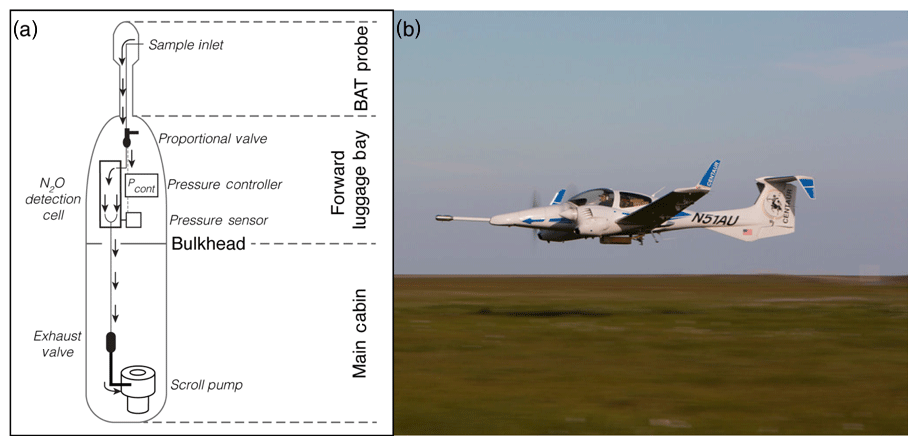
Figure 1FOCAL during flight. (a) Top-down schematic of the atmospheric gas flow through the aircraft (not to scale). The sample inlet is situated on the BAT probe, located at the nose of the plane. The gas is pumped through the pressure-regulated detection cell of the ICOS spectrometer, located within the luggage bay in front of the pilot. (b) Image of the Diamond DA42 flying around 15 m above the surface.
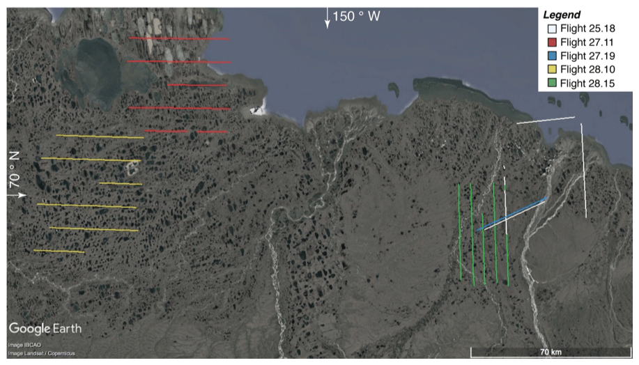
Figure 2Flight tracks for the August 2013 campaign, where the paths represent sections of the flights that were suitable for flux calculations (aircraft flying on a straight, level path below 50 m). (Map image credit: Google Earth).
To evaluate landscape N2O fluxes in the North Slope, the Flux Observations of Carbon from an Airborne Laboratory (FOCAL) system (shown in Fig. 1) was flown out of Deadhorse Airport, Prudhoe Bay, AK. Although its name comes from its ability to measure CO2 and CH4 fluxes, it can also simultaneously measure N2O flux. Measurements were made over five separate flights in several regions of the North Slope from 25 to 28 August 2013. The measurements entailed a cumulative path length of 884 km and approximate area coverage of 310 km2 (Fig. 2, Table 1). Flights consisted of straight flight tracks between 25 and 50 km long, some of which were upwind of a CH4∕H2O EC flux tower. For each flight, the flux calculations were restricted to straight segments flown below 50 m a.g.l. For the present study, segment sections over the open ocean were also excised.
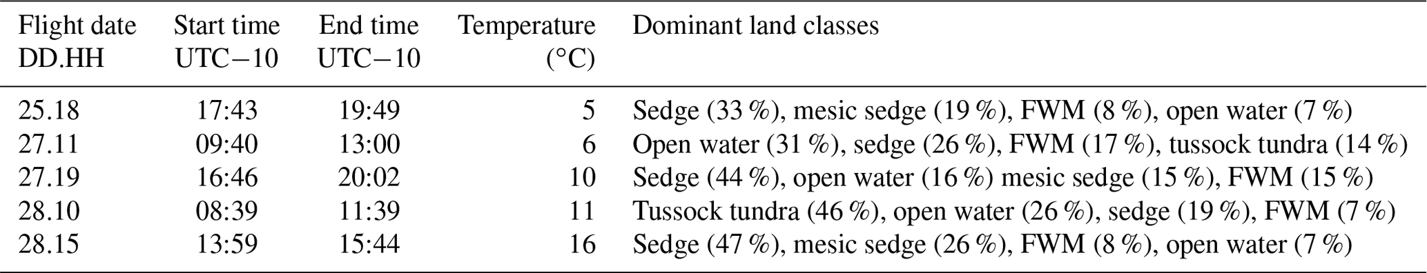
Table 1Description of the August 2013 flights. Flight date is the day of the flight in August (DD) and the “middle time” of flight to the nearest hour (HH). Temperature is the air temperature measured during the flight, averaged over all measurements made below 100 m. The dominant land classes are listed in order of decreasing relative contribution to the observed fluxes, determined by footprint analysis coupled with a land cover map. (FWM refers to fresh water marsh).
The low-flying aircraft flown in the campaign, a Diamond DA42 from Aurora Flight Sciences, housed the two main components for flux measurements (Fig. 1): a turbulence probe and a custom-built IR spectrometer measuring water vapor, CH4, and N2O at a rate of 10 times per second (10 Hz). These two components were used to measure the EC fluxes of N2O, CH4, and H2O during the 2013 campaign.
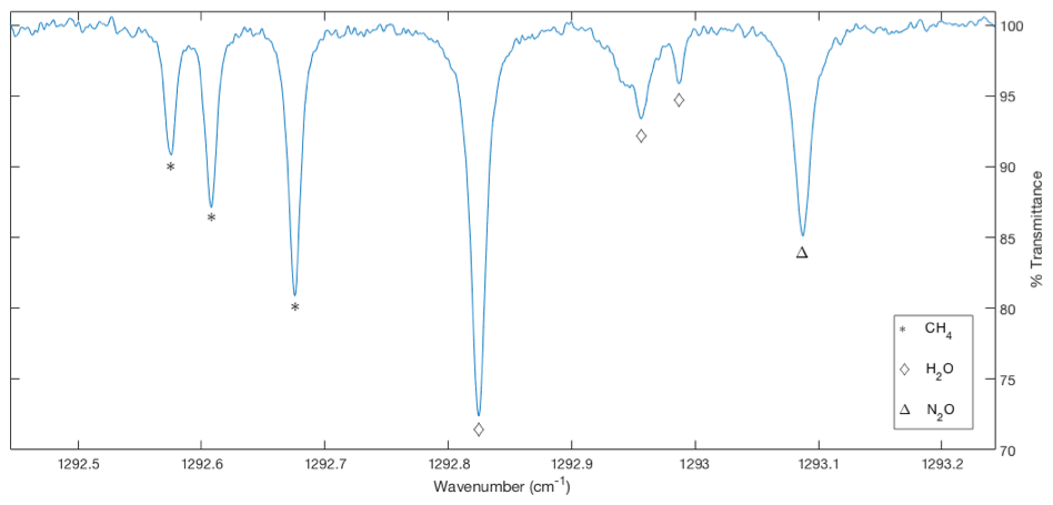
The flights near the flux tower were performed to compare the airborne CH4 and H2O flux measurements with those from the EC flux tower (Dobosy et al., 2017). The CH4 and H2O fluxes agreed with the ground measurement, and the CH4 fluxes are consistent with other observed summertime permafrost CH4 emissions reported in the scientific literature (see Sayres et al., 2017). The only difference in the airborne flux measurements between CH4, H2O, and N2O is the particular absorption feature used within the observed spectral region of the IR instrument, as further discussed in Sect. 2.2 (Fig. 3).
2.1 BAT probe description and calibration
The three wind components were measured using the Best Airborne Turbulence (BAT) probe developed by the National Oceanic and Atmospheric Administration/Atmospheric Turbulence and Diffusion Division (NOAA/ATDD) in collaboration with Airborne Research Australia (Crawford et al., 1993; Dobosy et al., 2013). The BAT probe also recorded ambient temperature and pressure measurements, which were used to determine dry-air density. The aircraft was equipped with a radar altimeter, which in conjunction with three-component wind velocity measurements, was used for footprint calculations. These calculations were performed over 60 m segments along the flight track (Sayres et al., 2017). The footprints, representing the area from which the observed fluxes originated, were used to estimate the total area measured and identify which land classes were measured (Table 1).
The BAT probe, developed in the 1990s, is a type of gust probe consisting of a hemispherical head, 15.5 cm in diameter, with ports at selected positions on the hemisphere to sample the pressure distribution. A gust probe functions similarly to a typical pitot-static system but includes additional pressure measurements to sense the direction of the incoming flow along with its speed. The direction is specified in two perpendicular components called angles of attack and sideslip, which rarely exceed in balanced flight (Leise et al., 2013). The BAT probe differs from other gust probes in that it has a larger head to accommodate accelerometers and pressure sensors directly in the head, simplifying the physical and mathematical system needed to determine turbulent wind. It also has nine ports instead of the usual five found in traditional gust-probe systems. These additional four ports measure the ambient atmospheric pressure apart from small adjustments for nonzero attack and sideslip angles. Wind is sampled at 1000 Hz, filtered to control aliasing, and subsampled at 50 Hz.
The BAT probe configured for the FOCAL campaign (with the gas inlets in place) was characterized in a wind tunnel (Dobosy et al., 2013) following on from an earlier wind-tunnel test of a similar unit in Indiana, USA (Garman et al., 2006). Its overall precision for wind is ±0.1 m s−1. With the entire instrument system assembled, standard-practice calibration maneuvers were flown in smooth air to establish the values of the tuning parameters for temperature, pressure, and wind measurement (Vellinga et al., 2013). Following the usual practice, we also made a calibration flight in smooth air on August 27 toward the end of the campaign (Sayres et al., 2017). Plots and comparison of spectra, cospectra, and time series for each flight provide tests of the quality of the data and of the processing through all intermediate steps.
2.2 N2O instrument description and calibration
The gas inlet for the N2O instrument is located on the BAT probe housing, 8 cm aft of the probe's hemispherical face, where ambient pressure and temperature measurements are made. The custom-built IR instrument uses off-axis integrated cavity output spectroscopy (OA-ICOS) to simultaneously measure H2O, CH4, and N2O (Figs. 4 and S1 in the Supplement). The light source is a distributed feedback (DFB) continuous-wave quantum cascade laser (QCL) (Hamamatsu, LC0349). The laser tunes from 1292.5 to 1293.3 cm−1 in 1.6 milliseconds. This region contains absorption features for H2O, CH4, and N2O (Fig. 3). Before the light enters the optical cavity, a beam-splitter diverts some of it through a Ge etalon. The etalon measures the rate at which the laser is tuning across the wavelength region, which is used to determine the width of the absorption lines. These components are all housed in the laser pressure vessel (Healy, 2016).
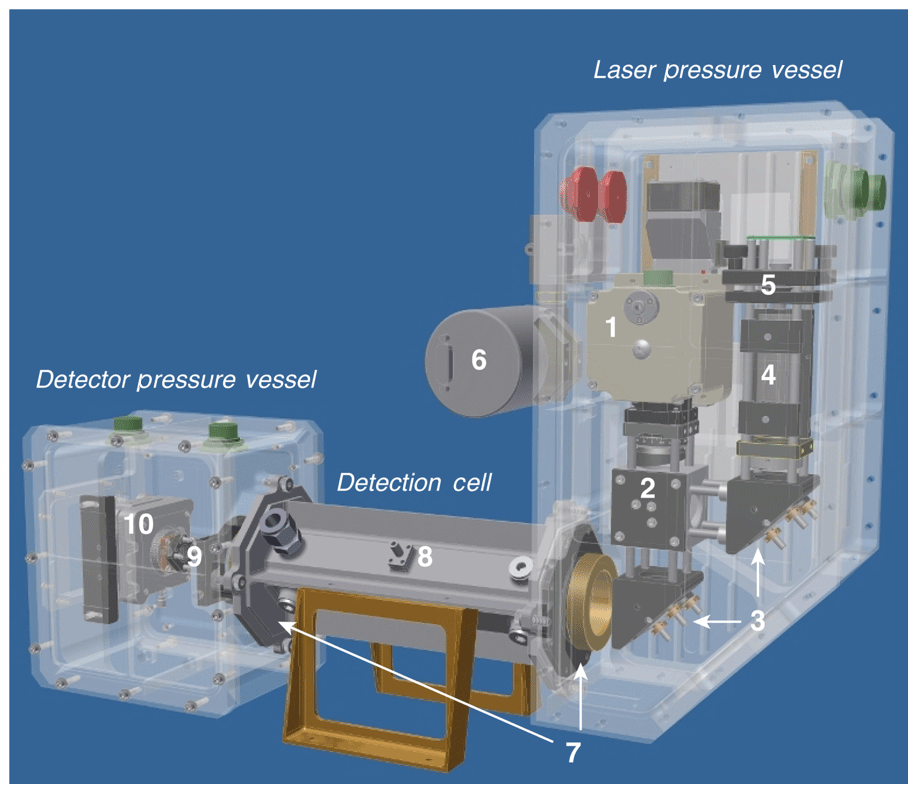
Figure 4CAD model of ICOS instrument shows (1) quantum cascade laser housing, (2) beam splitter, (3) steering optics, (4) Ge etalon, (5) etalon detector, (6) Baratron pressure sensor, (7) ICOS cavity mirrors, (8) temperature sensor port, (9) focusing optics, and (10) MCT detector. The detection cell is 25 cm long.
The detection cell is a 25 cm length optical cavity composed of two high-reflectivity ZnSe mirrors (LohnStar Optics, R=0.9996), which creates an effective path length of ∼625 m. After leaving the cavity, the light enters the detector pressure vessel where it is focused onto a Stirling-cooled HgCdTe photoconductive detector (InfraRed Associates, Inc., MCT-12-2.05C). The detector system samples the light at 100 MHz and averages the readings to produce raw spectra with 1900 samples each. These spectra are then co-added to produce 1 spectrum every 0.1 s and are stored on the flight computer.
Sample flow through the optical cavity is maintained in flight with a dry scroll pump that flushes the cell 17 times per second. The optical cavity is temperature- and pressure-controlled to K and Torr to allow conversion from concentration (moles cm−3) to mixing ratio. The cell temperature is measured by averaging the output of two 1 MΩ thermistors (General Electric, Type B) located within the cell. These were calibrated against a platinum primary standard. The cell is heated by polyimide thermofoil heaters, which are located along the cell exterior. The cell pressure is measured with a dual-headed absolute pressure transducer (MKS, D27D) and is controlled by a proportional solenoid valve. The valve is coupled with a pressure control board that uses the pressure transducer as feedback on the valve orifice's position (Fig. 1a) (Healy, 2016).
Measurement of H2O was calibrated using a dry-air tank coupled with a bubbler flow system as described in Weinstock et al. (2009). The H2O measurements were used to account for dilution and water-broadening effects on the N2O absorption feature and to convert the mixing ratio from moles per mole of total air to moles per mole of dry air for flux computation (Webb et al., 1980; Gu et al., 2012). The broadening coefficients were determined using the approach described in Rella (2010).
Periodic in-flight calibrations were performed to track and correct for drift over the course of the flight (two calibration cycles per flight). These were performed using a secondary standard (277 ppbv N2O) calibrated in the lab to a WMO standard (Sayres et al., 2017). Before and after the campaign, calibrations were also conducted in the lab using two primary WMO standards and a synthetic air tank (containing no N2O) to calibrate the absorption coefficient and check for linearity. The short-term precision of the ICOS instrument for N2O mixing ratios is determined using
where σ1 s is the 1 s standard deviation for in-flight calibration data collected during that particular flight, and fs is the sampling frequency in Hz (Kroon et al., 2007). Optical alignment was occasionally adjusted between flight days resulting in an N2O precision range over the five flights of σ=0.27–0.58 ppb Hz (Table S1 in the Supplement). This is close to the recommended precision for N2O EC flux measurements as determined by previous studies evaluating the application of the EC technique to this particular trace gas; these groups also used QCL spectroscopy to measure N2O mixing ratios (Kroon et al., 2007; Eugster et al., 2007).
2.3 Airborne EC flux calculations
The airborne EC method relies on the fact that gases like H2O, CH4, and N2O emitted from the surface are transported upward into the atmospheric boundary layer by turbulent eddies. On average, upward flux occurs when updrafts are, more often than not, enriched in the transported gas relative to downdrafts. Thus, the covariance of vertical wind velocity with gas concentration is positive (negative) for upward (downward) flux.
To determine the covariance between vertical wind velocity w and N2O mixing ratios c, we first separate each variable into changes associated with large-scale air motion (i.e., advection) and small-scale air motion, i.e., turbulence (e.g., ). We separated the two scales by fitting fourth-order polynomials to the measurements of w and c made along each individual straight leg of each flight (Fig. 2). The fit itself incorporates the larger-scale trends (e.g., ), which are subtracted from the data. The remaining residuals from this fit are the turbulent quantities of interest (e.g., w′) (Foken, 2008).
By multiplying w by the density of dry air ρd and extracting the residual as discussed above, one obtains the turbulent dry-air mass flux. The covariance of this dry-air flux (ρdw)′ with the turbulent mixing ratio c′ then yields the trace-gas flux of interest by the general EC approach (Webb et al., 1980; Gu et al., 2012):
As previously mentioned, airborne EC measurements average over space instead of time. Accordingly, we compute the N2O fluxes (along with CH4 and H2O fluxes) using the general equation for airborne EC flux calculations:
where V is the airspeed of the aircraft, and the other variables are defined as in Eq. (2) (Sayres et al., 2017; Dobosy et al., 2017). The true airspeed is included in Eq. (3) to convert the variable of integration from time to space because the raw data are recorded at uniformly spaced time intervals (every 0.1 s) (Crawford et al., 1993). A number N of samples is averaged, with the denominator yielding their cumulative path length through the air.
Air density and vertical wind velocity w from the BAT probe are filtered and then subsampled at 10 Hz to match the measurement frequency for , , and . Because the BAT probe observes a specific packet of air before the spectrometer does, a correction for the lag is applied to the data. The lag time from the gas inlet to the optical cavity was measured in the laboratory to be around 0.55 s. The lag between the BAT-probe measurements and those of the ICOS instrument in flight were determined by a cross-correlation analysis of w and . They varied between 0.4 and 1.2 s. Methane was used as a proxy for N2O to determine the lag because of its stronger signal.
Computation of dry-air density uses the measured dry-air mixing ratio of H2O. Turbulent quantities required for the footprint model are then computed by summing Eq. (3) over each flight segment. The mean N2O fluxes displayed in Table 2 are computed by summing Eq. (3) over the multiple segments of each flight depicted in Fig. 2, excluding flight-path sections over coastal waters.
2.4 Flux uncertainty analysis
All confidence intervals reported in Tables 2 and S1 are derived using bootstrap resampling (Dobosy et al., 2017), not from w and individually but from flux fragments (Sayres et al., 2017; Dobosy et al., 2017). These fragments are short (typically 1 s) blocks of integrated data that include the integrals of the three wind components, the height above ground, and the cross products of turbulent departure quantities from Eq. (3). All are integrated as above – over the path through the air rather than time. They are each about 60 m long and vary slightly due to small airspeed changes. These measurements, and therefore the corresponding confidence intervals, contain both environmental variability and variability arising from instrumental noise.
The fragments are serially correlated, and their means, trends, and variances are heterogeneous on scales greater than the 6 km found by ogive analysis to belong to turbulence. A procedure described by Mudelsee (2010) decomposes such partially determined, autocorrelated, and variably spaced data streams using the equation
Here X(S) is a random-variable function over the path length S defined at irregular intervals (Mudelsee, 2010). The T(S) and σ(S) are the respective deterministic trend and variance of X(S) for each S, and R(S) is a serially correlated random-variable series with a zero mean and unit variance. The T(S) and σ(S) for the current analysis are estimated as overlapping averages and variances of the measured fragments taken over 6 km, as determined by ogive analysis. They are evaluated at intervals of 1 km along the track and treated as fixed throughout the rest of the process. These larger scales can be treated as determinable from some (mesoscale) model.
The serial correlation of the random series R(S) is removed by a first-order Markov model, the inverse of a first-order causal filter (Dobosy et al., 2017). The resulting decorrelated series is (ideally) independent and “weakly” homogeneous (i.e., it has zero mean and unit variance). As such, it is suitable for bootstrap resampling. A resample size of 80 000 random decorrelated sequences, each the same length as the original set of fragments was drawn. The explained portion of the variance was then reapplied to each new resample using a process that is the reverse of the process of its removal; this process provided an ensemble of 80 000 new potential outcomes of the original experiment. The confidence intervals for N2O flux were determined from the distribution of this population of reconstituted potential outcomes.
A Student's t test was also used to evaluate whether the Pearson correlation coefficient for w′ and , and hence the N2O flux, differs significantly from a random (zero) correlation (Eugster and Merbold, 2015). Because the atmospheric data stream is serially correlated, as noted above, the N samples do not represent the total number of independent samples n. The number of independent samples is determined by
where ρ1 is the lag-1 autocorrelation coefficient (Eugster and Merbold, 2015). The conclusions of this test are incorporated into Table 2.
2.5 Footprint and land class determination
Following Sayres et al. (2017), the model developed by Kljun et al. (2004) is used to derive a footprint for each 60 m flux fragment. The wind and height above ground level are averaged over the fragment, and the required turbulence quantities are averaged over the flight leg containing the fragment. This procedure accounts for variations in mean wind and height above ground along the track while using the longer average required for flux computation. The footprints are used to estimate each flux fragment's related source area on the surface. The set union of these source areas constitutes the total area covered by each flight. Each flux fragment's coverage area is estimated by multiplying the length accounting for 90 % of the crosswind-integrated probability in the footprint by the path length of the respective flux fragment. For flights 25.18 and 27.19, the aircraft sometimes flies over the same path multiple times during the same flight. In these cases, the observed area is only counted once. These areas are summed for all of the fragments in each flight (Table 2).
For determining the land classes associated with the flux footprints, we use a land cover map developed by the North Slope Science Initiative (NSSI); there were 24 land classes used for the NSSI classification scheme (NSSI, 2013). However, for our land classification, the following land classes are conflated: tussock tundra and tussock shrub tundra; freshwater marsh Arctophila fulva and freshwater marsh Carex Aquatillis; dwarf shrub – Dryas and dwarf shrub – other; ice/snow and open water.
3.1 Cospectra and ogives
A cospectrum, the spectral decomposition of the covariance of the vertical wind velocity and trace gas mixing ratio, reveals the contribution to the overall flux from turbulent eddies as a function of their size. Starting from the smallest scales, the cospectrum normally increases to a maximum and then returns to near zero, sometimes increasing again at still larger scales. The cumulative integral of the cospectrum up to its first return to zero is known as the ogive. The cospectra and ogives averaged over the entire campaign are shown for H2O, CH4, and N2O in Fig. 5.
Table 2Observed flux averages. The area covered is the footprint scope of the measurements made for each flight. Spatially averaged fluxes are presented with the bootstrap-derived 90 % confidence intervals in parentheses. Asterisks indicate that the mean flux is significantly greater than 0 µg N2O m−2 s−1 (p<0.01).
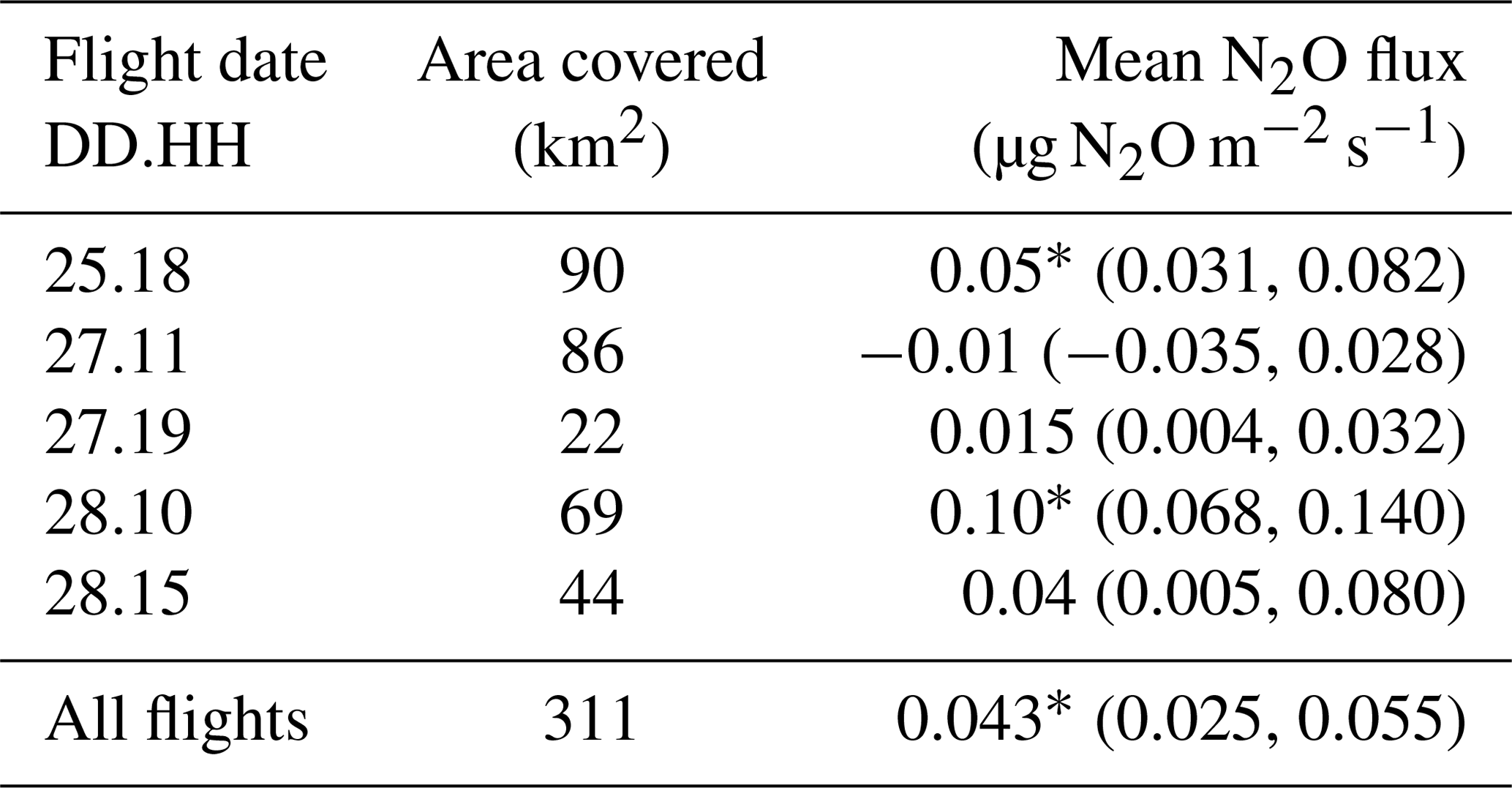
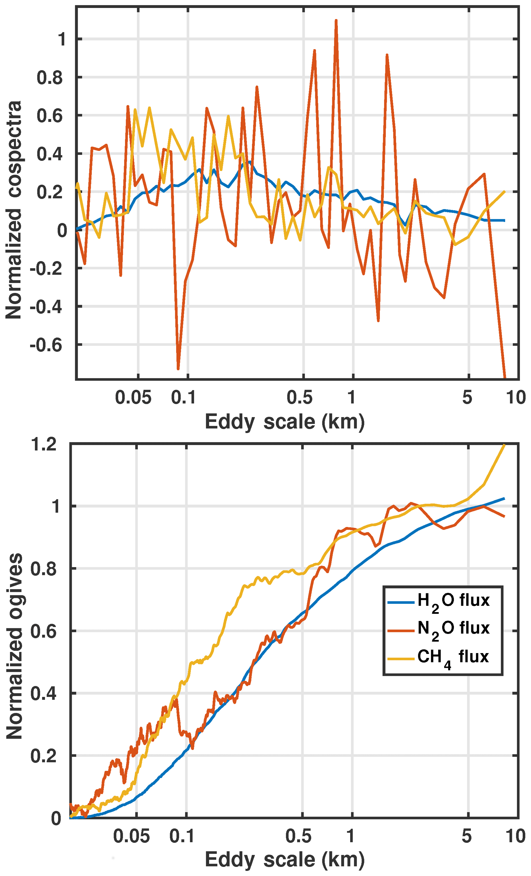
Figure 5Normalized average cospectra and ogives for the H2O flux, N2O flux, and CH4 flux. The average covers the entire flight campaign. The ogive integration starts from the smallest eddy sizes.
The usual cospectrum has the shape of the H2O flux (Fig. 5, blue). This cospectrum reaches a peak around 300 m, above which the incremental contribution to the flux declines with increasing eddy scale reaching near zero in this case at about 6 km. This length is taken to be the largest scale of boundary-layer turbulence for H2O. Therefore, it is the minimum averaging length for H2O fluxes. For the ogive, this point corresponds to the inflection point (zero slope). The cospectrum and ogive curves are normalized by the value of the ogive at its inflection point. Thus, the ogive reaches unity at its inflection point, where it is proportional to the mean flux density (g m−2 s−1) of H2O.
The cospectra of the remaining two gases (CH4 and N2O) follow the same pattern but with considerably more scatter due to the weaker flux of these gases, among other things. The ogive of N2O in particular shows notably strong contributions from the smaller scales (below 80 m) and the larger scales (above 500 m), perhaps resulting from a spotty distribution of sources (e.g., Fig. 6). The maximum turbulent scales for CH4 and N2O were taken from these ogives to be 4 and 6 km, respectively.
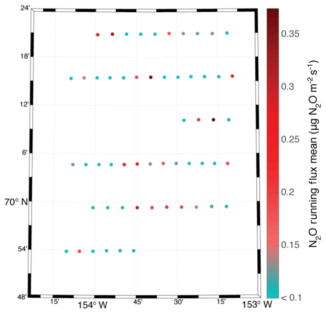
Figure 6Spatial flux map for Flight 28.10, where the circles on the map each represent the N2O flux averaged over 6 km with a 3 km overlap. Values within ±0.1 µg N2O m−2 s−1 are treated as zero.
3.2 Spatial distribution of N2O flux
Figure 6 shows a spatial map of N2O emissions measured during Flight 28.10. The individual points represent running averages obtained by summing Eq. (3) over 6 km paths with a 3 km overlap. The choice of a 6 km averaging length for Flight 28.10 was determined by ogive analysis as discussed above (Foken, 2008).
The detection limit for observing these 6 km average N2O fluxes was estimated by computing the running averages using Eq. (3) as described above but replacing the measured environmental with a synthetic vector of the same length (∼55 min). The synthetic vector was assembled by random resampling with replacement from 3 min (1800 samples) of N2O mixing ratios obtained during the same flight from a cylinder with a known N2O mixing ratio. All other data streams, such as ρd and w, containing both instrumental and environmental variability, remained unchanged. These 6 km running averages composed of calibration data had a mean value of 0.0±0.05 µg N2O m−2 s−1. We use 2σ to define the instrumental uncertainty of the 6 km averages and treat 6 km average values of ±0.1 µg N2O m−2 s−1 in Fig. 6 as indistinguishable from zero.
While Flight 28.10 had a significant overall average emission (Table 2), Fig. 6 illustrates that much of that emission arises in multiple small-scale domains (commonly referred to as “hot spots”) with approximately half of the 6 km means being indistinguishable from zero given the instrumental uncertainty described above. This hot-spot pattern is true for the other flights as well. This highlights the spatiotemporal variability of soil N2O emissions and could help explain why permafrost N2O emission studies, which are sparse and rely on extremely small spatial sampling when undertaken, often detect no significant flux (Kroon et al., 2007; Butterbach-Bahl et al., 2013).
3.3 N2O flux averages
The whole-flight spatially averaged N2O fluxes for each flight and the approximate surface area covered are shown in Table 2. Several of the averages are higher than have been previously assumed for N2O emissions at these latitudes. For example, the average N2O flux from tundra is considered to be around 0.005 µg N2O m−2 s−1 (Potter et al., 1996). In contrast, the whole-flight average from Flight 28.10, dominantly from tussock tundra (Table 1), was 0.104 µg N2O m−2 s−1, which is 20 times higher than the assumed value. Of the five flights, there are two flights where the average agrees with the expectation of negligible emissions (flights 27.11 and 27.19). The flight where we observed the lowest average N2O flux, Flight 27.11, covered land surfaces significantly more waterlogged than the other flights (Table 1). This observation is consistent with the established understanding that water saturation acts as a suppressant of N2O emissions because N2O is instead anaerobically processed into N2 by nitrous oxide reductase, an enzyme hypothesized to be inhibited by O2 (Morley et al., 2008; Butterbach-Bahl et al., 2013.
Explaining the low mean flux for Flight 27.19 is less straightforward. Even though the path of Flight 27.19 was in the same proximity as flights 25.18 and 28.15, Flight 27.19 has a noticeably lower average than the other two (which have similar mean fluxes; Table 2). Because this was an evening flight under reduced solar radiation, the boundary layer may have been too shallow to communicate the full emission of N2O from the surface to the flight level where it could be measured (Sayres et al., 2017). Separately, Table 1 shows that the ordering of the land classes measured was the same for all three flights. However, Flight 27.19's contribution from lakes and freshwater marsh was higher than from the other flights in that area (Sayres et al., 2017). Therefore, the comparatively lower average could also be a consequence of that flight's footprints covering a higher fraction of waterlogged environments.
The mean flux for all flights is 0.043 µg N2O m−2 s−1 (Table 2). This average is significantly different from zero flux (p<0.01) as determined by both bootstrap-derived CIs and the Student's t test as described in Sect. 2 (see Table S1 for 99 % CI ranges). This corresponds to a daily mean between 2.2 and 4.7 mg N2O m−2 d−1 (this range represents the 90 % CI values in Table 2 being converted to mg N2O m−2 d−1). These observed N2O emissions are higher than expected (Zhuang et al., 2012). However, there have been several small-scale chamber studies that have observed N2O emissions within this mean daily range (Repo et al., 2009; Marushchak et al., 2011; Yang et al., 2018). Soil analyses on the North Slope thermokarst features in upland tundra have also found elevated soil N2O concentrations sustained throughout the growing season (Abbott and Jones, 2015). These elevated levels were attributed to abrupt thaw processes known as thermokarst, which can cause permafrost to collapse. This displaced soil redistributes soil organic matter into both oxic and anoxic environments, a condition conducive to producing N2O as a final product instead of as a metabolic intermediate for N2 (Abbott and Jones, 2015). Transitions, in general, from oxic to anoxic environments (and vice versa) are well-known to induce spikes in N2O emissions for a variety of soils (Schreiber et al., 2012).
If results from the last week of August are representative of the whole month, the N2O emission over the span of August is ∼0.04–0.09 g N m−2. This range contains what is currently assumed to be the maximum emission over an entire year at these latitudes (∼0.05 g N m−2 yr−1) (Anderson et al., 2010; Zhuang et al., 2012). Past static chamber studies and soil studies that measured elevated permafrost N2O production observed that it was sustained throughout the entire growing period, which spans several months. One of these studies (Abbott and Jones, 2015) specifically examined permafrost in the North Slope, as we did in our campaign. Furthermore, these studies largely attribute the elevated rate of soil N2O production to higher soil temperatures (Repo et al., 2009; Abbott and Jones, 2015). Soil temperatures taken near our flux tower were lower during our observation period than in previous weeks of August 2013 (Fig. S2).
A body of evidence suggests the nutrient composition of, and microbial communities within, permafrost soils can be conducive to N2O production. Boreal peat soils are known to have negligible N2O emissions when the soil C∕N ratios are above 25 (Klemedtsson et al., 2005). However, below this threshold, N2O fluxes can increase quite rapidly with decreasing C∕N ratios. For the upper 3 m of permafrost, all three subsets of permafrost soils (Histel, Turbel, and Orthel) have mean C∕N ratios below 25, with Turbel soils averaging the lowest at ∼15 (Harden et al., 2012). Importantly, these values are averaged over many studies; the C∕N ratio is highly variable. For example, eight yedoma (organic-rich permafrost soil) and thermokarst sites in Arctic Siberia were reported to have C∕N ratios of 11, averaged over a 3 m depth (Fuchs et al., 2018). To reiterate, the upper 3 m is relevant for permafrost collapse, which routinely exposes deeper soil to the atmosphere. Furthermore, as discussed in a review of permafrost microbiology by Jansson and Taş (2014), metagenomic analyses (analyses quantifying relative abundance of genes in an environmental sample) performed on permafrost cores suggest N2O is likely the final product for denitrification. This is due to the fact that while most of the genes for the denitrification pathway were observed, the relative abundance of genes corresponding to the final steps was determined to be too low to lead to any significant conversion of N2O to N2 (Jansson and Taş, 2014).
It is unclear whether these observed emissions signify a recent trend or have been constant over time because the data collected on permafrost N2O fluxes are severely limited. No estimate of permafrost N2O emissions before the industrial revolution exists, and few data have been collected since (Davidson and Kanter, 2014). Therefore, it is unknown how these emissions have changed since global climate change started significantly affecting the permafrost landscape. However, it is well established that the troposphere at these higher latitudes has warmed, on average, 1.9 times more than the global average (Serreze and Barry, 2011). Soil temperatures have increased as well. Temperatures of permafrost soils in northern Alaska, for example, have increased by up to 3 ∘C since the 1980s (IPCC, 2013). Permafrost warming/thaw, independent of permafrost collapse, has been demonstrated to increase N2O emissions significantly (Elberling et al., 2010; Voigt et al., 2016, 2017). Furthermore, this temperature increase has induced permafrost degradation over time, which has manifested as the expansion of thermokarst features that have been shown to promote elevated N2O production even further as discussed above. Finally, increased permafrost thaw may make soil drainage more efficient, thus reducing the extent of waterlogged environments in higher latitudes (Avis et al., 2011). More streamlined draining also allows for a greater extent of draining and rewetting of permafrost soils, a process shown to increase thawed permafrost emissions of N2O 10-fold (Elberling et al., 2010). All of the observed changes to permafrost discussed above are variables that have been examined with respect to N2O emissions, and they have all have been shown to increase the fluxes of this gas. Based on this existing literature, our observed N2O emissions may reflect a positive climate feedback already in progress. That being said, it is unclear to what extent future emission rates will increase because soil temperature is only one of many factors that will continue to change at high latitudes, with increasing vegetation being the most likely to negate the effects of increasing soil temperatures (Repo et al., 2009; Voigt et al., 2017).
In this campaign, we flew over ∼310 km2 of the Alaskan North Slope and measured N2O flux using the airborne eddy-covariance technique. We observed spotty spatial distribution of elevated N2O emissions that averaged to 0.043 (0.025, 0.055) µg N2O m−2 s−1. These results corroborate several recent studies that have used the static chamber method and observed permafrost soils emitting significant levels of N2O that are sustained throughout the entire growing period. This is in contrast to the traditional view regarding emissions at these latitudes. Importantly, we corroborate these findings in a complementary way: we observe fluxes on a landscape scale rather than using the much smaller-scale soil plots seen in chamber studies, which are intended more to understand temporal representativeness and mechanisms of N2O production. While our study spans a spatial coverage greater by orders of magnitude than any previous study, it is still preliminary. The Arctic/sub-Arctic covers a vast area, and our observations do not necessarily represent the entire growing period (which is months long). This limitation notwithstanding, we demonstrate that it is possible to apply the established airborne EC technique to the trace gas N2O to more thoroughly evaluate emissions of N2O in permafrost regions. This approach is a useful supplement as most of the landscape is remote and inhospitable, making maintenance of flux towers and chambers intractable.
Climate projection models and stratospheric ozone depletion assessments rely on global N2O budgets to predict future atmospheric scenarios (Ravishankara et al., 2009; Meinshausen et al., 2011). Considering the observed N2O fluxes reported here, more field campaigns that employ the airborne EC technique or similar measurement techniques designed for much larger spatial coverage should be employed. These should also be coupled with ground-based measurements that can help corroborate airborne findings and better pinpoint where elevated N2O emissions might be occurring. Finally, future research efforts should consider following in the monitoring footsteps of CO2 and CH4 and establish continuously measuring EC towers for permafrost N2O. Campaigns like these would help better determine whether the current, data-limited assumption of negligible N2O emissions is a correct one. If permafrost N2O emissions are already not negligible, their predicted increase with warming permafrost soil temperatures could result in a non-carbon climate feedback of a currently unanticipated magnitude.
The datasets generated and analyzed during the current study are available at https://doi.org/10.7910/DVN/YM70Y7 (Sayres and Dobosy, 2018).
The supplement related to this article is available online at: https://doi.org/10.5194/acp-19-4257-2019-supplement.
BB, RD, DSS, and JGA designed the study. DSS, ED, and CH contributed to instrument development, data collection, and field work. JW and RD contributed to data processing and uncertainty analysis. JW was mainly responsible for interpreting the results and writing the paper. All authors participated in writing/editing the paper.
The authors declare that they have no conflict of interest.
We thank Marco Rivero, Norton Allen, and Chris Tuozolo for their laboratory and field assistance; Bernard Charlemagne for piloting the aircraft; and Jessica B. Smith, Eileen Moisson, and Andrew Bendelsmith for their comments on the paper. This work was funded by NSF grant no. 1203583.
This paper was edited by Eliza Harris and reviewed by two anonymous referees.
Abbott, B. W. and Jones, J. B.: Permafrost collapse alters soil carbon stocks, respiration, CH4, and N2O in upland tundra, Glob. Change Biol., 21, 4570–4587, https://doi.org/10.1111/gcb.13069, 2015.
Anderson, B., Bartlett, K., Frolking, S., Hayhoe, K., Jenkins, J., and Salas, W.: Methane and Nitrous Oxide Emissions from Natural Sources, Office of Atmospheric Programs, US EPA, EPA 430-R-10-001, Washington DC, 2010.
Avis, C. A., Weaver, A. J., and Meissner, K. J.: Reduction in areal extent of high-latitude wetlands in response to permafrost thaw, Nat. Geosci., 4, 444–448, https://doi.org/10.1038/ngeo1160, 2011.
Borge, A. F., Westermann, S., Solheim, I., and Etzelmüller, B.: Strong degradation of palsas and peat plateaus in northern Norway during the last 60 years, The Cryosphere, 11, 1–16, https://doi.org/10.5194/tc-11-1-2017, 2017.
Butterbach-Bahl, K., Baggs, E. M., Dannenmann, M., Kiese, R., and Zechmeister-Boltenstern, S.: Nitrous oxide emissions from soils: how well do we understand the processes and their controls?, Philos. T. R. Soc. B, 368, 20130122–20130122, https://doi.org/10.1098/rstb.2013.0122, 2013.
Crawford, T., McMillen, R., Dobosy, R., and MacPherson, I.: Correcting airborne flux measurements for aircraft speed variation, Bound.-Lay. Meteorol., 66, 237–245, 1993.
Davidson, E. A. and Kanter, D.: Inventories and scenarios of nitrous oxide emissions, Environ. Res. Lett., 9, 105012, https://doi.org/10.1088/1748-9326/9/10/105012, 2014.
Dobosy, R., Dumas, E., and Senn, D.: Calibration and Quality Assurance of an Airborne Turbulence Probe in an Aeronautical Wind Tunnel, J. Atmos. Ocean. Tech., 30, 182–196, https://doi.org/10.1175/JTECH-D-11-00206.1, 2013.
Dobosy, R., Sayres, D., Healy, C., Dumas, E., Heuer, M., Kochendorfer, J., Baker, B., and Anderson, J. G.: Estimating random uncertainty in airborne flux measurements over Alaskan tundra: Update in the Flux-Fragment Method, J. Atmos. Ocean. Tech., 34, 1807–1822, https://doi.org/10.1175/JTECH-D-16-0187.1, 2017.
Elberling, B., Christiansen, H. H., and Hansen, B. U.: High nitrous oxide production from thawing permafrost, Nat. Geosci., 3, 332–335, https://doi.org/10.1038/ngeo893, 2010.
Eugster, W. and Merbold, L.: Eddy covariance for quantifying trace gas fluxes from soils, SOIL, 1, 187–205, https://doi.org/10.5194/soil-1-187-2015, 2015.
Eugster, W., Zeyer, K., Zeeman, M., Michna, P., Zingg, A., Buchmann, N., and Emmenegger, L.: Methodical study of nitrous oxide eddy covariance measurements using quantum cascade laser spectrometery over a Swiss forest, Biogeosciences, 4, 927–939, https://doi.org/10.5194/bg-4-927-2007, 2007.
Foken, T.: Micrometeorology, 2nd edn., Springer-Verlag, Bayreuth, Germany, 113–115, 2008.
Fuchs, M., Grosse, G., Strauss, J., Günther, F., Grigoriev, M., Maximov, G. M., and Hugelius, G.: Carbon and nitrogen pools in thermokarst-affected permafrost landscapes in Arctic Siberia, Biogeosciences, 15, 953–971, https://doi.org/10.5194/bg-15-953-2018, 2018.
Garman, K., Hill, K. A., Wyss, P., Carlsen, M., Zimmerman, J. R., Stirm, B. H., Carney, T. Q., Santini, R., and Shepson, P. B.: An airborne and wind tunnel evaluation of a wind turbulence measurement system for aircraft-based flux measurements, J. Atmos. Ocean. Tech., 23, 1696–1708, https://doi.org/10.1175/JTECH1940, 2006.
Gioli, B., Miglietta, F., De Martino, B., Hutjes, R. W. A., Dolman, H. A. J., Lindroth, A., Schumacher, M., Sanz, M., Manca, G., Peressotti, A., and Dumas, E.: Comparison between tower and aircraft-based eddy covariance fluxes in five European regions, Agr. Forest Meteorol., 127, 1–16, https://doi.org/10.1016/j.agrformet.2004.08.004, 2004.
Gu, L., Massman, W. J., Leuning, R., Pallardy, S. G., Meyers, T., Hanson, P. J., Riggs, J. S., Hosman, K. P., and Yang, B.: The fundamental equation of eddy covariance and its application in flux measurements, Agr. Forest Meteorol., 152, 135–148, https://doi.org/10.1016/j.agrformet.2011.09.014, 2012.
Harden, J. W., Koven, C., Ping, C., Hugelius, G., McGuire, A. D., Camill, P., Jorgenson, T., Kuhry, P., Michaelson, G. J., O'Donnell, J. A., Schuur, E. A. G., Tarnocai, C., Johnson, K., and Grosse, G..: Field information links permafrost carbon to physical vulnerabilities of thawing, Geophys. Res. Lett., 39, 71–6, https://doi.org/10.1029/2012GL051958, 2012.
Healy, C.: Mapping and Characterizing the Alaskan North Slope Methane Flux With Airborne Eddy-Covariance Flux Measurements, PhD dissertation, Graduate School of Arts & Sciences, Harvard University, 2016.
Hensen, A., Skiba, U., and Famulari, D.: Low cost and state of the art methods to measure nitrous oxide emissions, Environ. Res. Lett., 8, 025022, https://doi.org/10.1088/1748-9326/8/2/025022, 2013.
IPCC: Climate Change 2013: The Physical Science Basis. Contribution of Working Group I to the Fifth Assessment Report of the Intergovernmental Panel on Climate Change, edited by: Stocker, T. F., Qin, D., Plattner, G.-K., Tignor, M., Allen, S. K., Boschung, J., Nauels, A., Xia, Y., Bex, V., and Midgley, P. M., Cambridge University Press, Cambridge, United Kingdom and New York, NY, USA, 1535 pp., https://doi.org/10.1017/CBO9781107415324, 2013.
Jansson, J. K. and Taş, N.: The microbial ecology of permafrost, Nat. Rev. Microbiol., 12, 414–425, https://doi.org/10.1038/nrmicro3262, 2014.
Jones, B. M., Baughman, C. A., Romanovsky, V. E., Parsekian, A. D., Babcock, E. L., Stephani, E., Jones, M. C., Grosse, G., and Berg, E. E.: Presence of rapidly degrading permafrost plateaus in south-central Alaska, The Cryosphere, 10, 2673–2692, https://doi.org/10.5194/tc-10-2673-2016, 2016.
Klemedtsson, L., Arnold, Von, K., Weslien, P., and Gundersen, P.: Soil CN ratio as a scalar parameter to predict nitrous oxide emissions, Glob. Change Biol., 11, 1142–1147, https://doi.org/10.1111/j.1365-2486.2005.00973.x, 2005.
Kljun, N., Calanca, P., Rotach, M., and Schmid, H.: A simple parameterization for flux footprint predictions, Bound.-Lay. Meteorol., 112, 503–523, https://doi.org/10.1023/B:BOUN.0000030653.71031.96, 2004.
Kroon, P. S., Hensen, A., Jonker, H. J. J., Zahniser, M. S., van 't Veen, W. H., and Vermeulen, A. T.: Suitability of quantum cascade laser spectroscopy for CH4 and N2O eddy covariance flux measurements, Biogeosciences, 4, 715–728, https://doi.org/10.5194/bg-4-715-2007, 2007.
Leise, J. A., Masters, J. M., and Dobosy, R. J.: National Oceanic and Atmospheric Association. Wind measurements from aircraft, NOAA technical memorandum OAR ARL-266, 209 pp., https://doi.org/10.7289/V5/TM-OAR-ARL-266, 2013.
Mahrt, L.: Flux Sampling Errors for Aircraft and Towers, J. Atmos. Ocean. Tech., 15, 416–428, https://doi.org/10.1175/1520-0426(1998)015<0416:FSEFAA>2.0.CO;2, 1998.
Martikainen, P. J., Nykänen, H., Crill, P., and Silvola, J.: Effect of a lowered water table on nitrous oxide fluxes from northern peatlands, Nature, 366, 51–53, 1993.
Marushchak, M. E., Pitkamaki, A., Koponen, H., Biasi, C., Seppala, M., and Martikainen, P. J.: Hot spots for nitrous oxide emissions found in different types of permafrost peatlands, Glob. Change Biol., 17, 2601–2614, https://doi.org/10.1111/j.1365-2486.2011.02442.x, 2011.
McGuire, A. D., Christensen, T. R., Hayes, D., Heroult, A., Euskirchen, E., Kimball, J. S., Koven, C., Lafleur, P., Miller, P. A., Oechel, W., Peylin, P., Williams, M., and Yi, Y.: An assessment of the carbon balance of Arctic tundra: comparisons among observations, process models, and atmospheric inversions, Biogeosciences, 9, 3185–3204, https://doi.org/10.5194/bg-9-3185-2012, 2012.
Meinshausen, M., Smith, S. J., Calvin, K., Daniel, J. S., Kainuma, M. L. T., Lamarque, J.-F., Matsumoto, K., Montzka, S. A., Raper, S. C. B., Riahi, K., Thomson, A., Velders, G. J. M., and van Vuuren, D. P. P.: The RCP greenhouse gas concentrations and their extensions from 1765 to 2300, Climatic Change, 109, 213–241, https://doi.org/10.1007/s10584-011-0156-z, 2011.
Morley, N., Baggs, E. M., Dörsch, P., and Bakken, L.: Production of NO, N2O and N2 by extracted soil bacteria, regulation by and O2 concentrations, FEMS Microbiol. Ecol., 65, 102–112, https://doi.org/10.1111/j.1574-6941.2008.00495.x, 2008.
Mudelsee, M.: Climate Time Series Analysis: Classical Statistical and Bootstrap Methods, 2nd edn., Springer, Cham, Switzerland, 474 pp., 2010.
North Slope Science Initiative: North Slope Science Initiative Landcover Mapping Summary Report, available at: http://catalog.northslopescience.org/catalog/entries/4616-nssi-landcover-report-landcover-mapping-for-north (last access: 27 January 2018), 2013.
Park, S., Boering, K. A., Etheridge, D. M., Ferretti, D., Fraser, P. J., Kim, K.-R., Krummel, P. B., Langenfelds, R. L., van Ommen, T. D., Steele, L. P., and Trudinger, C. M.: Trends and seasonal cycles in the isotopic composition of nitrous oxide since 1940, Nat. Geosci., 5, 261–265, https://doi.org/10.1038/ngeo1421, 2012.
Pihlatie, M. K., Kiese, R., Brüggemann, N., Butterbach-Bahl, K., Kieloaho, A.-J., Laurila, T., Lohila, A., Mammarella, I., Minkkinen, K., Penttilä, T., Schönborn, J., and Vesala, T.: Greenhouse gas fluxes in a drained peatland forest during spring frost-thaw event, Biogeosciences, 7, 1715–1727, https://doi.org/10.5194/bg-7-1715-2010, 2010.
Potter, C., Matson, P., Vitousek, P., and Davidson, E.: Process modeling of controls on nitrogen trace gas emissions from soils worldwide, J. Geophys. Res., 101, 1361–1377, https://doi.org/10.1029/95JD02028, 1996.
Rannik, Ü., Haapanala, S., Shurpali, N. J., Mammarella, I., Lind, S., Hyvönen, N., Peltola, O., Zahniser, M., Martikainen, P. J., and Vesala, T.: Intercomparison of fast response commercial gas analysers for nitrous oxide flux measurements under field conditions, Biogeosciences, 12, 415–432, https://doi.org/10.5194/bg-12-415-2015, 2015.
Ravishankara, A. R., Daniel, J. S., and Portmann, R. W.: Nitrous Oxide (N2O): The Dominant Ozone-Depleting Substance Emitted in the 21st Century, Science, 326, 123–125, https://doi.org/10.1126/science.1176985, 2009.
Rella, C.: Accurate Greenhouse Gas Measurements in Humid Gas Streams Using the Picarro G1301 Carbon Dioxide/Methane/Water Vapor Gas Analyzer, Picarro, Inc, Santa Clara, CA, USA, 2010.
Repo, M. E., Susiluoto, S., Lind, S. E., Jokinen, S., Elsakov, V., Biasi, C., Virtanen, T., and Martikainen, P.: Large N2O emissions from cryoturbated peat soil in tundra, Nat. Geosci., 2, 189–192, https://doi.org/10.1038/ngeo434, 2009.
Sayres, D. and Dobosy, R.: Alaska 2013 Campaign, Harvard Dataverse, V1, https://doi.org/10.7910/DVN/YM70Y7, 2018.
Sayres, D. S., Dobosy, R., Healy, C., Dumas, E., Kochendorfer, J., Munster, J., Wilkerson, J., Baker, B., and Anderson, J. G.: Arctic regional methane fluxes by ecotope as derived using eddy covariance from a low-flying aircraft, Atmos. Chem. Phys., 17, 8619–8633, https://doi.org/10.5194/acp-17-8619-2017, 2017.
Schreiber, F., Wunderlin, P., Udert, K. M., and Wells, G. F.: Nitric oxide and nitrous oxide turnover in natural and engineered microbial communities: biological pathways, chemical reactions, and novel technologies, Front. Microbiol., 3, 1–24, https://doi.org/10.3389/fmicb.2012.00372, 2012.
Sellers, P., Hall, F., Kelly, R. D., Black, A., Baldocchi, D., Berry, J., Ryan, M., Ranson, K. J., Crill, P. M., Lettenmaier, D. P., Margolis, H., Cihlar, J., Newcomer, J., Fitzjarrald, D., Jarvis, P. G., Gower, S. T., Halliwell, D., Williams, D., Goodison, B., Wickland, D. E., and Guertin, F. E.: BOREAS in 1997: Experiment overview, scientific results, and future directions, J. Geophys. Res., 102, 28731–28769, https://doi.org/10.1029/97JD03300, 1997.
Serreze, M. C. and Barry, R. G.: Processes and impacts of Arctic amplification: A research synthesis, Global Planet. Change, 77, 85–96, https://doi.org/10.1016/j.gloplacha.2011.03.004, 2011.
Syakila, A. and Kroeze, C.: The global nitrous oxide budget revisited, Greenhouse Gas Measurement and Management, 1, 17–26, https://doi.org/10.3763/ghgmm.2010.0007, 2011.
Vellinga, O., Dobosy, R., Dumas, E. J., Gioli, B., Elbers, J. A., and Hutjes, R. W. A..: Calibration and quality assurance of flux observations from a small research aircraft, J. Atmos. Ocean. Tech., 30, 161–181, https://doi.org/10.1175/JTECH-D-11-00138.1, 2013.
Voigt, C., Lamprecht, R. E., Marushchak, M. E., Lind, S. E., Novakovskiy, A., Aurela, M., Martikainen, P. J., and Biasi, C.: Warming of subarctic tundra increases emissions of all three important greenhouse gases – carbon dioxide, methane, and nitrous oxide, Glob. Change Biol., 23, 3121–3138, https://doi.org/10.1111/gcb.13563, 2016.
Voigt, C., Marushchak, M. E., Lamprecht, R. E., Jackowicz-Korczyński, M., Lindgren, A., Mastepanov, M., Granlund, L., Christensen, T., Tahvanainen, T., Martikainen, P. J., and Biasi, C.: Increased nitrous oxide emissions from Arctic peatlands after permafrost thaw, P. Natl. Acad. Sci. USA, 114, 6238–6243, https://doi.org/10.1073/pnas.1702902114, 2017.
Webb, E., Pearman, G., and Leuning, R.: Correction of flux measurements for density effects due to heat and water vapour transfer, Q. J. Roy. Meteor. Soc., 106, 85–100, https://doi.org/10.1002/qj.49710644707, 1980.
Weinstock, E., Smith, J. B., Sayres, D. S., Pittman, J. V., Spackman, J. R., Hinsta, E. J., Hanisco, T. F., Moyer, E. J., St. Clair, J. M., Sargent, M. R., and Anderson, J. G.: Validation of the Harvard Lyman-α in situ water vapor instrument: Implications for the mechanism that control stratospheric water vapor, J. Geophys. Res., 114, D23301, https://doi.org/10.1029/2009JD012427, 2009.
Yang, G., Peng, Y., Marushchak, M.E., Chen, Y., Wang, G., Li, F., Zhang, D., Wang, J., Yu, J., Liu, L., Qin, S., Kou, D., and Yang, Y.: Magnitude and Pathways of Increased Nitrous Oxide Emissions from Uplands Following Permafrost Thaw, Environ. Sci. Technol., 52, 9162–9169, https://doi.org/10.1021/acs.est.8b02271, 2018.
Zhuang, Q., Lu, Y., and Chen, M.: An inventory of global N2O emissions from the soils of natural terrestrial ecosystems, Atmos. Environ., 47, 66–75, 2012.
Zona, D., Jannsens, I.A., Aubinet, M., Gioli, B., Vicca, S., Fichot, R., and Ceulemans, R.: Fluxes of the greenhouse gases (CO2, CH4 and N2O) above a short-rotation poplar plantation after conversion from agricultural land, Agr. Forest Meteorol., 164, 100–110, https://doi.org/10.1016/j.agrformet.2012.10.008, 2013.