the Creative Commons Attribution 4.0 License.
the Creative Commons Attribution 4.0 License.
 | 03 Apr 2019
Indications for a potential synchronization between the phase evolution of the Madden–Julian oscillation and the solar 27-day cycle
Christoph G. Hoffmann
Christian von Savigny
The Madden–Julian oscillation (MJO) is a major source of intraseasonal variability in the troposphere. Recently, studies have indicated that also the solar 27-day variability could cause variability in the troposphere. Furthermore, it has been indicated that both sources could be linked, and particularly that the occurrence of strong MJO events could be modulated by the solar 27-day cycle.
In this paper, we analyze whether the temporal evolution of the MJO phases could also be linked to the solar 27-day cycle. We basically count the occurrences of particular MJO phases as a function of time lag after the solar 27-day extrema in about 38 years of MJO data. Furthermore, we develop a quantification approach to measure the strength of such a possible relationship and use this to compare the behavior for different atmospheric conditions and different datasets, among others. The significance of the results is estimated based on different variants of the Monte Carlo approach, which are also compared.
We find indications for a synchronization between the MJO phase evolution and the solar 27-day cycle, which are most notable under certain conditions: MJO events with a strength greater than 0.5, during the easterly phase of the quasi-biennial oscillation, and during boreal winter. The MJO appears to cycle through its eight phases within two solar 27-day cycles. The phase relation between the MJO and the solar variation appears to be such that the MJO predominantly transitions from phase 8 to 1 or from phase 4 and 5 during the solar 27-day minimum. These results strongly depend on the MJO index used such that the synchronization is most clearly seen when using univariate indices like the OLR-based MJO index (OMI) in the analysis but can hardly be seen with multivariate indices like the real-time multivariate MJO index (RMM). One possible explanation could be that the synchronization pattern is encoded particularly in the underlying outgoing longwave radiation (OLR) data. A weaker dependence of the results on the underlying solar proxy is also observed but not further investigated.
Although we think that these initial indications are already worth noting, we do not claim to unambiguously prove this relationship in the present study, neither in a statistical nor in a causal sense. Instead, we challenge these initial findings ourselves in detail by varying underlying datasets and methods and critically discuss resulting open questions to lay a solid foundation for further research.
- Article
(4534 KB) -
Supplement
(213 KB) - BibTeX
- EndNote


The solar electromagnetic radiation is the major energy source of the earth system. Although usually described with the solar constant (1361 W m−2), the total solar irradiance (TSI) is subject to variations on different timescales, with the most prominent one being the solar 11-year cycle. While the variation of the TSI is only on the order of 0.1 %, it differs among the spectral regions and is particularly strong in the UV (e.g., Coddington et al., 2015, and references therein). Of interest for the present study is the solar 27-day cycle, which is a combined result of the differential rotation of the sun and irradiance inhomogeneities on the solar disc. The amplitude of the 27-day cycle is generally smaller than that of the 11-year cycle, but can be on the order of 50 % of the 11-year amplitude in the UV during strong events. The 27-day cycle is not perfectly periodic, but exhibits some variability, so that the 27 days have to be seen as a mean period of a quasi-periodic process. When using terms like the “solar cycle”, “solar maximum”, etc., we always refer to the 27-day variations in this paper if not stated otherwise.
The solar variations introduce atmospheric variability and many effects have been identified in the past, particularly in the middle atmosphere, where the strongly varying UV is important. Signatures of the 27-day cycle have been found in, for example, temperature (Hood, 1986; von Savigny et al., 2012; Thomas et al., 2015), trace gases (e.g., Hood, 1986; Robert et al., 2010; Thomas et al., 2015; Fytterer et al., 2015; Lednyts'kyy et al., 2017), polar mesospheric clouds (e.g., Robert et al., 2010; Thurairajah et al., 2017; Köhnke et al., 2018), and very recently in radio wave reflection heights (von Savigny et al., 2019). The interactions between solar and atmospheric variability are still subject to ongoing research, which aims at both identifying more affected parameters and elucidating the underlying mechanisms. The attribution of 27-day signals in the atmosphere to a solar cause is thereby complicated by the fact that internal variability of the atmosphere can itself also produce signals with periods around 27 days, as pointed out by, for example, Sukhodolov et al. (2017), which becomes even more important for lower altitudes.
Nevertheless, in addition to implications in the middle atmosphere, a discussion of possible of 27-day signatures in the troposphere came up recently, mostly in the context of convection and clouds (Takahashi et al., 2010; Hong et al., 2011; Miyahara et al., 2017; Hood, 2018), but also related to temperature (Hood, 2016). Even more than for the middle atmospheric effects, questions concerning the mechanisms behind tropospheric signatures arise. Two major classes of conceivable mechanisms are summarized by Hood (2018) and mentioned here only briefly: on the one hand the “bottom-up” mechanisms (detailed by Meehl et al., 2008, 2009), which assume that the only slight variations of the TSI produce strong enough heating changes directly in the troposphere to generate the observed modulations in the upper troposphere, and on the other hand the “top-down” mechanisms, which consider the stratospheric effects of the stronger UV variations as starting point. The modulations could result via a chain of effects in a change of upper tropospheric static stability and with that in a change of tropospheric deep convection, with implications for clouds and temperature. Another mechanism, particularly for a connection between clouds and the solar variability, has been proposed in a few variants (e.g., Svensmark, 1998; Marsh and Svensmark, 2000) but has also been heavily criticized (e.g., Damon and Laut, 2011) and is mentioned here only for completeness. It considers a connection of cloud condensation nuclei and incoming galactic cosmic rays, whose flux is affected by solar activity.
Independent of a possible solar influence, there is a known important source of tropospheric variability on the intraseasonal timescale, the Madden–Julian oscillation (MJO). It was first reported by Madden and Julian (1972), and more recent reviews of properties and implications are found in Zhang (2005) and Lau and Waliser (2012). In brief, it is a planetary-scale pattern in the tropics consisting of a region with anomalous strong deep convection flanked by two regions of weak deep convection to the east and to the west. This pattern evolves over the Indian Ocean and travels eastward across the Maritime Continent until it decays in the Pacific. This temporal evolution is usually split into eight phases as originally suggested by Madden and Julian (1972, Fig. 16). The MJO pattern reappears periodically; however, the period is strongly variable in a range between 30 and 100 days (Zhang, 2005). The MJO is the dominant component of intraseasonal variability in the tropical troposphere with strong influences on rainfall and the genesis of tropical cyclones in the respective regions, for example. In addition, there are also increasing indications for an entanglement of the MJO in teleconnections and, hence, for an influence of the MJO in the extratropics (e.g., Garfinkel et al., 2014). Due to its intraseasonal timescale and the large spatial scales, one important motivation for MJO research is that it could help to push the limits of weather forecasting skills towards longer periods (Zhang, 2013).
In addition to the tropospheric implications, indications for interdependencies with the middle atmosphere have also been brought up, particularly with ozone and temperature (e.g., Tian et al., 2007; Zhang et al., 2015; Yang et al., 2017). Of particular interest for the present study is the finding that the MJO depends on the state of quasi-biennial oscillation (QBO) (e.g., Son et al., 2016; Yoo and Son, 2016; Marshall et al., 2017). The QBO represents a quasi-periodic reversal of the stratospheric equatorial zonal winds with a mean period of 28 months (e.g., Baldwin et al., 2001). Briefly, it affects the MJO strength, particularly during boreal winter, such that the MJO is stronger during the QBO easterly phase.
In the context of solar-induced tropospheric variability there is a two-level interest in the MJO. First, it might be difficult to distinguish both possible causes for intraseasonal tropospheric variability, since the MJO acts on timescales (starting with 30 days) close to the solar 27-day variation. Hence, suspected 27-day signatures in the troposphere might in reality be connected to the MJO. Second, in the light of recent publications, which are outlined below, it appears at least conceivable that the MJO is itself influenced by the 27-day cycle. From this point of view, the MJO might be a pathway for the 27-day solar signal into the troposphere. Hence, the three topics solar 27-day variation, MJO, and tropospheric variability on intraseasonal timescales might be interconnected.
An example for the first level is the publication by Takahashi et al. (2010), which reports on 27-day variations found in the cloud amount over the western Pacific region. These results are based on a frequency analysis of OLR data in place of direct cloud amount data. The authors are cautious with speculating on possible mechanisms but also briefly mention that the spectral analysis shows indications of MJO activity and that some kind of interdependency cannot be ruled out.
The second level, a possible modulation of the MJO itself by the 27-day solar cycle, has been proposed by a series of studies (Hood, 2016, 2017, 2018). The study by Hood (2016) is actually focused on a tropospheric temperature response to solar 27-day variations. A modulation of the MJO is discussed as part of the mechanism, which brings the temperature signal into the troposphere. An initial investigation of this hypothesis shows a change of the occurrence of the particular MJO phases 1, 7, and 8 after solar 27-day extrema, which is considered to be consistent with the tropospheric temperature change. Hood (2017) directly deals with a solar modulation of the MJO, but is focused on the solar 11-year cycle and the occurrence rate of strong MJO events instead of MJO phase occurrences. The study indicates that the MJO is influenced by solar 11-year variations during boreal winter. This influence is roughly as important as the previously mentioned QBO modulation and might work with a similar mechanism: the modification of upper tropospheric stability. This also means that both influences have to work in the same direction (e.g., QBO easterly phase and solar minimum) to get a detectable MJO change. Hood (2018) also analyzes the occurrence of strong MJO events but returns to the solar 27-day variations. A statistical relationship between the solar 27-day variations and the occurrence of strong MJO events is indeed found during the boreal winter and spring months from December to May. Particularly, strong MJO events (amplitudes greater than 2) are decreased following solar maxima and vice versa. As before, this effect is stronger under QBO east conditions.
The analysis presented here contributes to the critical examination of a possible linkage between the solar 27-day cycle and the MJO based on the analysis of about 38 years of MJO data. It is complementary to the previous studies, as it deals with the temporal MJO phase evolution instead of MJO strength. Analyzing the temporal evolution focuses on a special aspect: the relation of the periods of both processes; first, the range of possible MJO periods starts close to the period of the solar 27-day cycle. And second, the mean periodicity of the MJO is with 50 to 60 days approximately twice that of the solar 27-day variability, which turns out to be of interest in the following. Overall, it is analyzed here if there are similarities and regularities in the temporal evolution of both processes and we will show that a kind of coincident behavior can indeed be found in a statistical sense, which is partly surprisingly clear. However, we would like to emphasize that we do not try to prove a causal relationship between the solar 27-day cycle and the MJO phase evolution at this early stage. Likewise, we do not try to establish a particular mechanism. Instead, we aim at describing the statistical features of a combined inspection of both quasi-period processes as a basis for future research.
In Sect. 2 we describe the analyzed datasets and the initial filtering of the data. In Sect. 3 the basic analysis idea is outlined first, before the essence of the statistical relationship found between the solar 27-day cycle and MJO phase evolution is demonstrated based on a particularly clear example. In Sect. 4 questions concerning the generalizability of this example are addressed. For this a numerical approach to measure the strength of the relationship is developed first, before the analysis is applied to different selections of the underlying data. A discussion of major open questions and the conclusions are found in Sect. 5.
Basically two pieces of information are needed to perform the present analysis: the time series of the solar activity and the MJO in the past.
The solar activity is represented by several proxy time series. We primarily use the Lyman alpha flux (Woods et al., 2000) as an indicator for solar activity. In addition, we have also performed the same analysis with the F10.7 radio flux index (e.g., Tapping and Charrois, 1994, and references therein) and UV radiation at 205.5 nm simulated by the NRLSSI2 model (Coddington et al., 2015), as well as similar data from a previous model version.
Many different indices have been developed to compactly describe the strength and phase of the MJO at a given time. These indices are usually calculated from either circulation data or information on cloudiness. The latter is usually represented by outgoing longwave radiation (OLR) data. Some approaches also combine both aspects to form multivariate indices (Straub, 2013). One of the latter indices is the real-time multivariate MJO index (RMM), which became the standard after its publication by Wheeler and Hendon (2004). A variant of RMM is the velocity potential MJO index (VPM) introduced by Ventrice et al. (2013), in which the OLR information is replaced by a velocity potential. This leads to a better MJO representation during boreal summer, among other advantages. More recently, Kiladis et al. (2014) introduced the OLR-based MJO index (OMI), which is a univariate index solely based on OLR data. It overcomes drawbacks of RMM (Straub, 2013; Kiladis et al., 2014) at the expense of the real-time capability. This disadvantage is, however, not of importance for retrospective analyses, so that OMI has become an important index at least for these cases. Kiladis et al. (2014) also introduce a second univariate OLR-based index, the filtered MJO OLR index (FMO), which is easier to calculate than OMI. Kiladis et al. (2014) point out that all these different indices lead to similar results concerning the statistical gross features of the MJO, but differences are to be expected when working on the basis of individual MJO events.
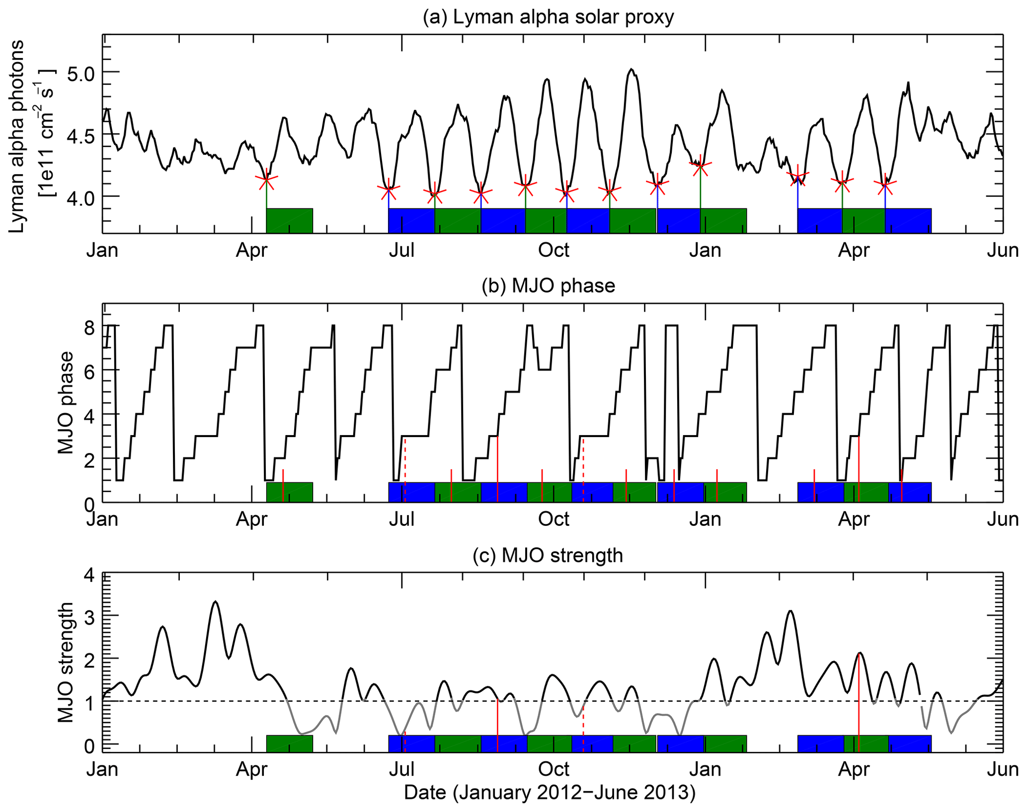
Figure 1Examples of the analyzed time series for the period January 2012 to June 2013. The Lyman alpha solar proxy (a) shows pronounced 27-day variability, particularly in the middle of this period. The MJO phase evolution (b; here represented by the OMI index) shows the expected periodic transitions from phase 1 to phase 8. However, it is obvious that the solar 27-day signal as well as the MJO phase evolution are definitely not perfectly periodic, but have to be considered as quasi-periodic processes (see Sect. 1). Strong variability also appears in the MJO strength (c, OMI index). The figure also indicates the basic steps of the analysis routine: identified solar minima are marked with red stars in the top panel. The resulting 0- to 28-day time lag epochs are indicated by alternating green and blue shaded areas in all three panels. As an example of the following counting step, it is illustrated how often MJO phase 3 occurred 10 days after solar minimum. For this, all 10-day time lags are marked (all vertical red lines in panel b). During 4 of these days, the MJO was in phase 3 (longer solid and dashed red lines). However, only days during which the MJO strength exceeded a particular threshold (here 1, horizontal dashed line in panel c) are considered so that the analysis results in two occurrences of phase 3 for time lag 10 (longer solid vertical red lines).
Since our analysis does not depend on real-time information, we use primarily the OMI index. An example of the OMI data as well as of the Lyman alpha solar proxy is shown in Fig. 1. Additionally, we have also applied our analysis to the RMM index, the VPM index, and the FMO index. All these indices provide two coefficients each, which are transformed into MJO phase and strength by basically applying a transformation from Cartesian coordinates, in which the index coefficients are given, to polar coordinates. The radius and phase angle of the polar coordinates then correspond to the MJO strength and phase, respectively. Note that there are different conventions among the different indices for the attribution of the index coefficients to the Cartesian coordinate system (Kiladis et al., 2014). The phase angle is then divided into eight ranges of 45∘ each, which represent the eight MJO phases mentioned before (e.g., Wheeler and Hendon, 2004).
The availability of the MJO indices is the limiting factor for the temporal extent of the analysis. The OMI index starts in 1979 and ends in August of 2017 at the time of the analysis and hence covers about 38 years. The other MJO indices cover roughly a similar period. All datasets are available with daily resolution so that the analysis is performed on a daily resolved grid.
As part of the analyses described in Sects. 3 and 4, the datasets are filtered with respect to geophysical properties: first, only days during which the MJO strength exceeds a particular threshold are considered. Second, as the marker for the start of a new solar 27-day cycle, the solar minimum is used mostly, but the solar maximum can also be selected. Third, from the detected solar cycles, the relevant ones can be selected according to the season and, fourth, they can be filtered according to the state of the QBO. For the latter, 50 hPa (and 30 hPa as alternative) zonal wind data from radiosondes in the tropics have been used (Naujokat, 1986). For the determination of the QBO phase, simply the sign of the wind data is used with positive values denoting the westerly phase and negative values denoting the easterly phase.
As the basic analysis step, we check whether individual MJO phases appear preferentially at a particular state of the solar 27-day cycle. The idea is to count the number of occurrences of the individual MJO phases as a function of time lag after solar extrema. We analyze 28 days after each solar extremum; these temporal windows are called the epochs. This analysis is related to the approach of Hood (2016), but we treat all eight MJO phases separately, while Hood (2016) focused on a combination of a few of them. We will demonstrate in the following that a preference for particular MJO phases depending on the solar 27-day state appears indeed to be present under certain conditions. We chose an experimental setup in this section for demonstration purposes, with which this relationship appears comparatively clear, and we will discuss the ability to generalize these findings in Sect. 4.
The following explanation of the analysis approach is also illustrated in Fig. 1. The analysis starts with identifying the solar 27-day minima in the Lyman alpha solar proxy time series (solar 27-day maxima are calculated likewise for other experimental setups). For this, the anomaly of the Lyman alpha time series is calculated by subtracting the smoothed time series (35-day moving average), which removes the variations greater than 35 days. Also the shorter-term variations are removed from the anomaly by smoothing it with a 5-day moving average. In the resulting proxy anomaly time series, the local extrema are identified. Only extrema with anomaly values of at least 0.2×10¹¹ photons cm−2 s−1 above or below 0 are considered. This is a relative conservative filtering of extrema candidates; to make sure that only clear cases are considered in the analysis, we risk that some actual extrema are missed by the algorithm. This approach leads therefore to a slight underrepresentation of solar 11-year minimum conditions, since 27-day minima are also less pronounced during these periods and are more likely to be rejected (quantitatively, no 27-day minima have been selected by the algorithm for Lyman alpha values below 3.57×10¹¹ photons cm−2 s−1, and a reduced 27-day minima selection is visually seen roughly below 3.8×10¹¹ photons cm−2 s−1). In total, the algorithm finds 243 solar minima in the 38-year period, which means that about 6500 days out of the about 14 000 days are covered with considered epochs. From this set only solar minima are selected, which occurred during boreal winter (December, January, February) and during the QBO easterly phase. This results in a set of only remaining 26 epochs. However, the filter criteria in this example are among the most restrictive ones, so that the number of 26 samples is roughly a lower boundary for the sample size of the following experiments.
For all remaining solar minima days, we count how often each of the eight MJO phases has occurred. A phase occurrence is only taken into account if the MJO strength exceeds the threshold of 1 in the current example, so that the sum of all phase occurrences is usually lower than the number of considered epochs (19 occurrences in this example). This is not only done for exactly those days with the solar minima, but it is repeated for all time lags between 1 and 28 full days after each solar minimum. This results in one curve for each of the eight MJO phases describing the number of occurrences as a function of time lag after solar minimum. These curves are shown for the current example in Fig. 2.
Considering that the MJO shows a great variability and that also the solar 27-day cycle is only a quasi-periodic process, one would expect that these curves are basically constant with strong noise contributions. This would mean that each MJO phase occurs without any preference similarly often at each time lag after the solar minimum, which in turn means that the MJO phases evolve independently of the solar 27-day cycle. And the first overall impression of the functions in Fig. 2 might apparently reflect this expected chaotic nature to a certain extent.
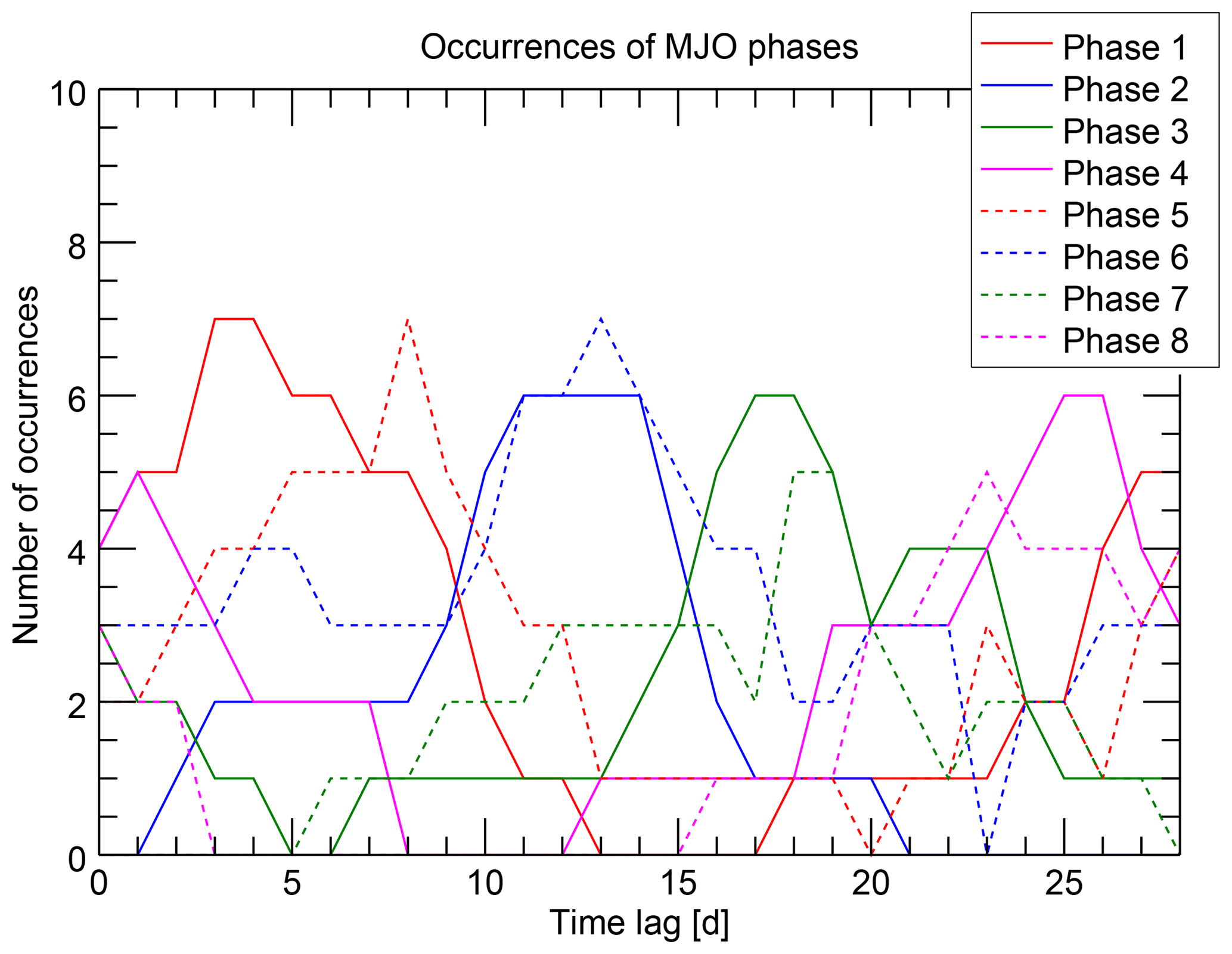
Figure 2Number of occurrences of each MJO phase (one line per phase) as a function of time lag after solar 27-day minima. The figure shows a particular example: only solar minima during boreal winter and during a QBO easterly phase were considered. After this filtering 26 epochs remain in the analysis. Furthermore, the MJO strength on individual days has to be greater than 1. The state of the MJO is characterized by the OMI index; the Lyman alpha solar proxy was used to determine the solar minima.
However, a closer look reveals some structure in the functions. First, each of the eight curves exhibits a maximum at a particular time lag. The maxima are partly quite pronounced (e.g., for MJO phase 1) and partly somewhat broader (e.g., for MJO phase 7), but a kind of maximum is recognizable for each of the MJO phases. This indicates that the MJO phases occur preferentially at a certain time lag after the solar minimum. Second, the positions of the maxima reveal a specific ordering. Starting with the maximum of MJO phase 1 at time lag 3 days, the maxima of the phases 2, 3, and 4 follow monotonically with increasing time lag. MJO phase 5 starts again with a low time lag of 8 days followed again monotonically by the phases 6, 7, and 8.
This structure is more clearly visualized in Fig. 3, where the time lags of the phase occurrence maxima are shown for each MJO phase. The two sequences of monotonically increasing time lags for the phases 1 to 4 and 5 to 8 are clearly visible and constitute a sawtooth-like pattern.
The appearance of this clear pattern is the major qualitative result of this study and the essential characterization of the possible relationship between the solar 27-day cycle and MJO phase evolution. We think that this result is quite remarkable considering that the MJO, although showing some kind of periodicity, is a highly variable phenomenon.
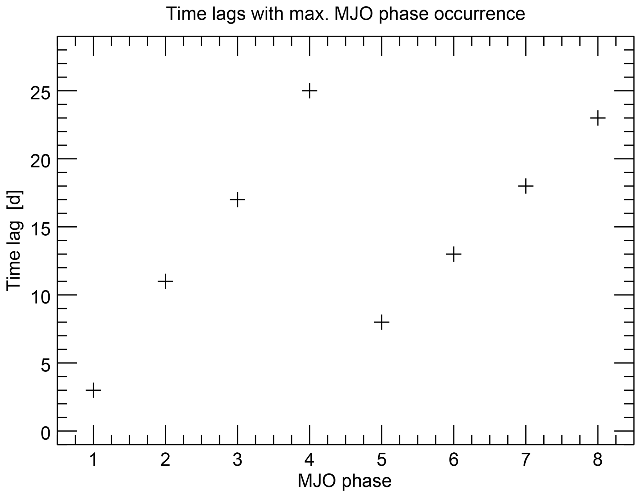
Figure 3Position of the maximum occurrence numbers (measured in time lag after solar minimum) for each MJO phase. Datasets and filtering conditions are similar to those in Fig. 2.
Based on the clearness of this pattern, it appears attractive to directly assume a causal synchronizing mechanism between the solar 27-day cycle and the MJO phase evolution, which would, however, be premature. Nevertheless, the mere appearance of this sawtooth pattern has at least two requirements. First, the mean period of the MJO should be twice as large as the mean period of the solar 27-day variation. Hence, it should be about 54 days, which is well in the already known range of periods. Taking into account, though, that the instantaneous MJO period varies strongly, the second requirement is needed, namely that there should be a predominant phase relation of the solar 27-day variations and the MJO phase evolution during the complete analyzed period, i.e., the MJO is predominantly around phase 1 or around phase 5 at solar minimum. Otherwise, the sawtooth shape would be arbitrarily shifted over the MJO phases for certain subperiods, so that the pattern would finally be averaged out when taking the complete analyzed period into account. These requirements are obviously to a large extent fulfilled in the present example; however, the question remains whether this fact really demands a causal mechanism or if it could also be a coincidence in the analyzed period. Furthermore, a possible causal mechanism would have to explain why the solar 27-day variation produces a variation with a doubled period, i.e., why there are two possible MJO phases at each solar state. We emphasize again that it is not our aim to prove such a causal connection in this study. Instead, we aim at carving out more statistical characteristics of this connection from the dataset itself in Sect. 4 as a first step. This helps to get a clearer picture of the conditions under which such a connection might exist.
In the light of the present findings, it is in order to briefly comment on some results in Hood (2016), which are also based on counting the occurrences of MJO phases as a function of time lag after solar 27-day maxima or minima. However, in contrast to the present study, the MJO phases are not treated individually, but only the cumulative occurrence of MJO phases 1, 7, and 8 is evaluated, which is motivated by the particular questions in this analysis. The author finds that the cumulative occurrence of these phases is enhanced in the days after solar minimum and reduced about 10 days after the solar minimum. With the present results in mind, it does not seem to be a very reasonable choice to combine the particular phases 1, 7, and 8 as their positions of maximum occurrence represent three (of possible four) different time lag ranges (Fig. 3). Instead, if one wants to group the phases with respect to the solar cycle, it would be more plausible to overlay the two lines of the sawtooth pattern, which means that the following pairs of MJO phases belong together in their relation to the solar 27-day cycle: 1 and 5, 2 and 6, 3 and 7, 4 and 8. Additionally, it should not be expected that the phase package 1, 7, and 8 behaves contrarily to the “opposite” phase package, consisting of the MJO phases 3, 4, and 5 (which Hood, 2016 does not claim, but what the reader might intuitively think). Instead this package represents similar maximum occurrence time lags as the first package 1, 7, and 8 (Fig. 3) and should behave similarly. With this in mind, the conclusions drawn based on these results in Hood (2016) should be reconsidered, especially because the author has pointed out the initial character of these results himself.
It is our aim to challenge the hypothesis of a relationship between the solar 27-day cycle and the MJO phase evolution by diversifying the setups of the numerical experiments. That means that the same analysis is repeated for different choices of atmospheric conditions, underlying datasets, and also implementation details. To do so, a quantity is needed first that measures the strength of the relationship and, hence, makes the results for different setups comparable.
4.1 Brief description of the quantification approach
Based on Fig. 3, it is intuitive to define such a quantity as the similarity of the pattern constituted by the eight data points to a sawtooth function. Numerically, this similarity can be estimated by fitting a sawtooth function to the data points. The goodness of fit χ2, which basically sums up the quadratic deviations between data points and the fitted sawtooth function, could then be a natural choice for such a measure; the smaller the value of χ2, the better the similarity to a sawtooth function and the stronger the relationship between the solar 27-day cycle and MJO evolution.
However, the common definition of χ2 has to be modified in two aspects to be a suitable measure in the present context. This is described in detail in Appendix Appendix A and mentioned here only briefly: first, the calculation of the individual deviations has to account for the fact that the time lags are periodic with a periodicity of 27 days. This is considered in the quantity defined in the Appendix A2. Second, the common weighting of each data point with its reverse variance works in the direction that a higher uncertainty (greater standard deviation σi) leads to a smaller χ2. This is useful for the numerical fitting routine, but works in the wrong direction for the present application, the measurement of deviations. For this application, a higher uncertainty should result in a greater value of the deviation, which reflects a weaker certainty of the relationship found. Both aspects are considered in the quantity X, which we defined as the measure of the deviation in the Appendix A3. This quantity X, simply called “deviation” in the following, is the measure used for the strength of the relationship in this study; a lower deviation indicates a stronger relationship between the solar 27-day cycle and the MJO phase evolution.
Altogether, our analysis routine comprises the following steps.
-
Performing the analysis steps described in Sects. 2 and 3. This consists of the following:
- a.
identification of the solar extrema dates,
- b.
filtering of the input data according to the experimental setup,
- c.
counting of the occurrences of the individual MJO phases as a function of time lag after the solar extrema,
- d.
identification of the time lags with maximum occurrence number for each MJO phase.
- a.
-
Estimation of the uncertainty of the derived time lags using a bootstrap method. This is described in more detail in Appendix A4.
-
Fitting the sawtooth function to the derived time lags of maximum occurrence for the eight MJO phases using the previously calculated bootstrap uncertainties as weights. As mentioned before, the fit is performed under consideration of the 27-day periodicity of the time lags, hence by minimizing instead of χ2. For the same reason, we have fixed the amplitude of the sawtooth function in the fit to a value of 27 days. Assuming, based on the previous results, that the mean periodicity of the MJO is with 54 days twice the mean periodicity of the solar 27-day cycle, we have also fixed the period to four MJO phases (only half of the eight MJO phases are experienced during one solar 27-day cycle). The only free parameter of the fit is the phase ϕSt of the sawtooth function. As the fitting routine might not directly find the global minimum of and, hence, the result might depend on the first guess of ϕSt, the fitting procedure is repeated with the first guesses of ϕSt systematically varied between 1 and 8. The result with the minimal is then considered further on.
-
Calculation of the measure of deviation X between data and fit using the bootstrap uncertainties as weights. Although the measure of the “deviation” is the direct quantitative result of the analysis, we are conceptually interested in the opposite, the “similarity” of the pattern in the data and the sawtooth function. In the following, we will use both terms equally in the sense that a small deviation means high similarity, which in turn means a stronger relation between the solar 27-day cycle and the MJO phase evolution. Furthermore, we will not put emphasis on the physical units of X, which depend on the weighting factors. Since only the variations in the results are of interest and not the absolute values, we will simply assume that X is given in arbitrary units.
-
Estimation of the significance of the quantified relationship. For this, the probability p that the value of the deviation X could be the product of only random features in the data is calculated. This is achieved with a Monte Carlo (MC) approach, which means that the input data are repeatedly modified with random numbers and the complete analysis procedure is applied to a large number (1000) of such randomly modified input data representations. The probability p is then simply calculated as the percentage of the random experiments, which resulted in a lower deviation measure. This probability value was then used to quantify the significance of the respective result; the lower the probability p that a low deviation can be reproduced with random numbers, the higher the significance of the result. We have implemented different possibilities for the creation of the random data. These are outlined together with the discussion of the respective results in Sect. 4.5. We use as the standard method in the following the most conservative implementation, i.e., the one that indicates significance of the results most rarely. This method is based on randomly shifting the original solar extrema dates by up to ±6 days and is also explained in more detail in Sect. 4.5.
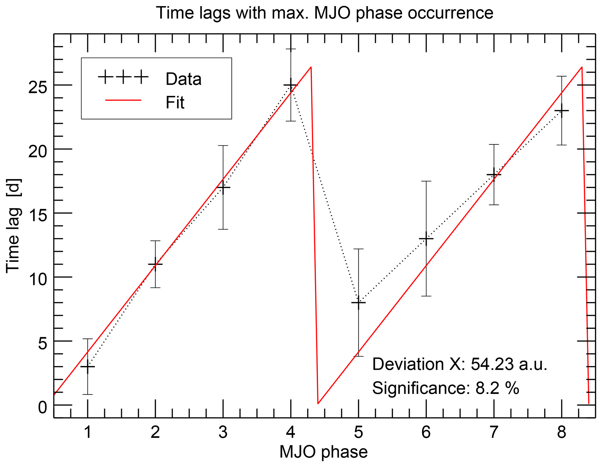
An example of the fitting process, which corresponds to the case previously discussed in Sect. 3, is shown in Fig. 4. More examples are included in the Supplement. After having performed this routine, a measure of the deviation between the sawtooth pattern in the empirical data and an analytical sawtooth function is known together with the fitted phase. This deviation characterizes the strength of a possible systematic relationship between the solar 27-day cycle and the MJO phase evolution. In the following, we will apply this approach to a variety of different experimental setups, which can then be compared among each other.
4.2 Influence of the numerical setup
Before we discuss the results in detail, we note that the analysis is, like most others, subject to well justified but strictly speaking arbitrary choices. Wherever possible, we have repeated the analysis with different realizations of these choices and have convinced ourselves that our main conclusions do not depend on these choices.
One choice is the definition of the epoch period. We have defined an epoch to start with a solar extremum and then last for 28 days. This is a natural choice, since – if any relation can be substantiated – we expect the sun to be the driver of the MJO phase evolution so that it makes sense to study the atmospheric response in the period after the solar extremum. However, a possible mechanism does not guaranty a direct response of the atmosphere in the following 28 days. Instead the response could also manifest itself during the solar cycles afterwards. Hence, no unambiguous starting point of an epoch can be fixed and it would also be possible to, for example, center the solar extremum in the epoch period, so that it covers the time lags from −14 to 14 days, like it is done in many studies. Interestingly, we found that some of our conclusions appear even clearer using this alternative choice of the epoch windows. Currently, we cannot decide whether this is a feature of the studied relationship, or if it is a random effect. Therefore, we decided to include the more conservative option of the 0- to 28-day epoch into the paper but show the alternative results in the Supplement.
Another choice is the use of squared weights in the definition of the deviation X as mentioned in Sect. A3. Hence, we have also repeated the calculations with constant weights (we have chosen , so that the sum over all 8 weights is unity), so that all data points are weighted with the same factor. Although these results are not interesting from an atmospheric point of view, we have also included them in the Supplement, to convince the reader that the conclusions are not influenced by the definition. However, for the interpretation of these alternative calculations, one has to note that the significance analysis cannot lead to very realistic results in the case of these arbitrary constant weights; since the values of these weights directly influence the value of X, the choice of weights directly influences the probability to gain a higher or lower X based on a random dataset. And whereas the original calculation of the weights considers the real spread of the data, leading to weights that actually characterize the dataset, the constant weights are completely unconnected with the dataset. What can still be seen from the results with constant weights is that the qualitative comparison of results with different experimental setups is similar and, hence, the conclusions are not dominated by the kind of weighting.
As an example, we have also included the results of both alternative calculations (the centered epoch definition as well as the constant weighting) in the presentation of the first experiment (Fig. 5, which is discussed in Sect. 4.3). Afterwards, all results will be based on the 0- to 28-day epoch and the squared bootstrap uncertainties as weights.
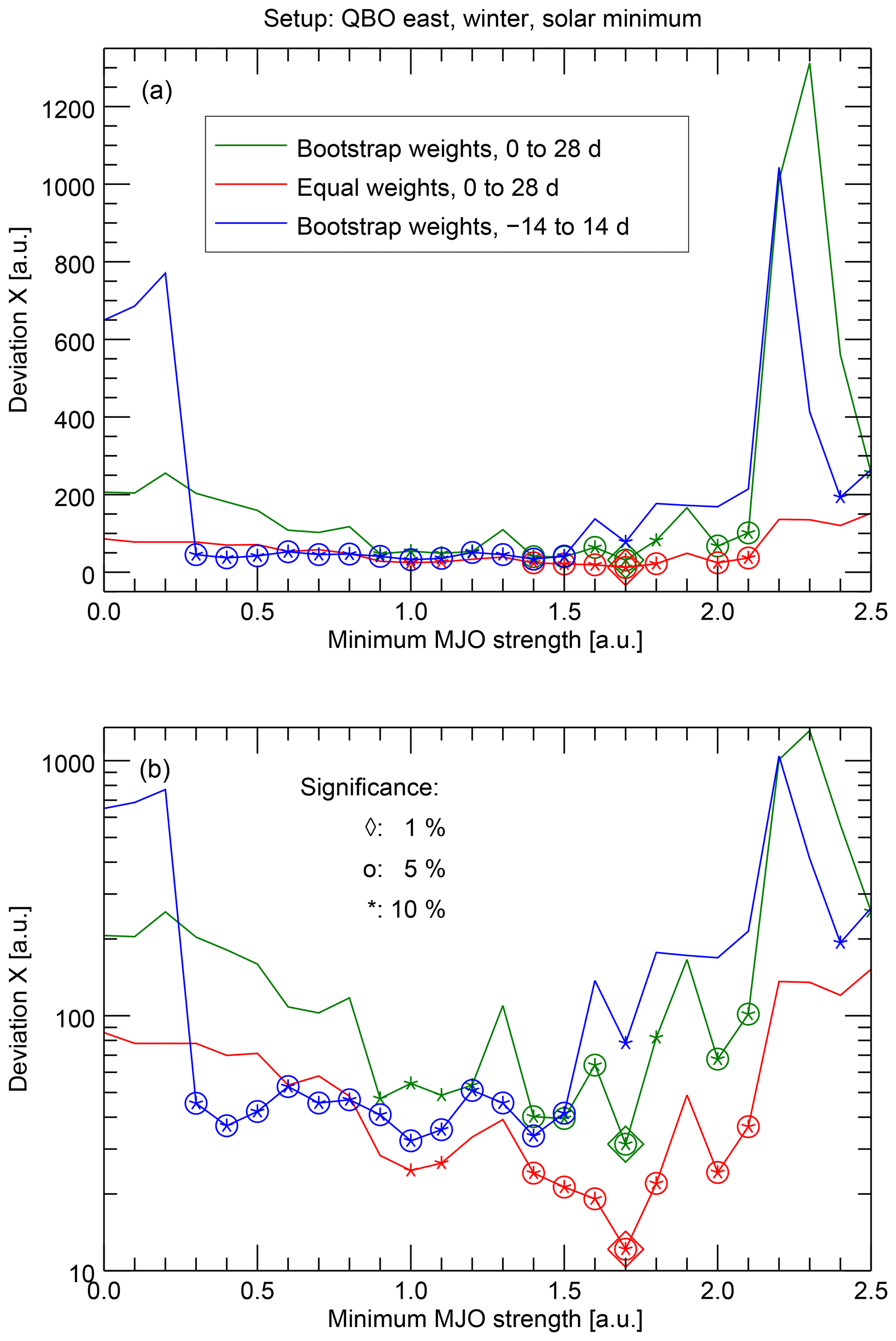
Figure 5Calculated deviations X indicating the strength of the statistical connection between the solar 27-day cycle and the MJO phase evolution; a lower X indicates a stronger connection. The same data are shown in linear scaling (a) for an overall visual impression and in logarithmic scaling (b) for inspection of the smaller variations. The focus of this experiment is the dependence of the deviation on the MJO strength threshold. The green line shows these results for the standard numerical setup. Three levels of significance in the sense of the MC experiment are shown: 10 %, 5 %, or 1 % chance of getting lower deviations with randomly modified solar extremum dates. The other two lines give an impression of the reaction of the results when the numerical setup is changed to, first, a different epoch definition (blue line) or, second, the use of constant weights (red line; see Sect. 4.2 for details).
4.3 Influence of atmospheric conditions
In the following experiments, one parameter of the analysis will be varied, while the others are kept constant with specific values. We used indications from pretests and previous studies, to choose standard values for the non-varied parameters, which lead to the clearest results and, hence, allow the best conclusions concerning the particular influence of the varied parameter. For the overall conclusions, the values of all filters have finally, of course, to be considered at the same time. An example of more relaxed filtering conditions is shown afterwards in Sect. 4.3.5. An overview of the varied parameters including the standard values in this and the following section (Sect. 4.4) is given in Table 1.
Table 1Parameters varied to quantify their influence on the possible relation between the solar 27-day cycle and the MJO phase evolution.

Note that it would also be interesting to study the influence of the 11-year solar cycle on the possible relationship between the solar 27-day cycle and the MJO phase evolution in addition to the variation of the parameters listed in Table 1. In principle, this is implemented in our analysis as one further filter; however, it turns out that the number of remaining samples becomes too small when this additional filter is applied. For the standard filtering conditions, the number of remaining solar 27-day cycles is already reduced to 19 (Sect. 3) and is halved by applying a solar 11-year maximum or minimum filter so that no significant and reliable conclusions can be drawn anymore. Therefore, this aspect has to remain open until longer datasets are available and one should keep in mind that the solar 11-year minimum conditions are slightly underrepresented in our analysis due to our 27-day extrema selection approach (Sect. 3).
4.3.1 MJO strength threshold
One major parameter for all MJO studies is the minimum MJO strength, which has to be reached for an MJO event to be considered. Very often, a value of 1 is used, sometimes also a value of 2. We have examined in more detail the influence of this threshold on our results first. For this we have varied the MJO strength threshold between 0 and 2.5 in 0.1 steps. The other filter criteria correspond to the standard of the example in Sect. 3. The results for the standard numerical setup are shown in Fig. 5 (green line).
The results show comparatively low deviations, i.e., stronger indications for a connection between the solar 27-day cycle and the MJO phase evolution, between thresholds of 0.8 and 2.1. In this center range, most of the results are significant at least at the 10 % level, many at the 5 % level, and some at the 1 % level. This means that the chance to derive lower deviations with randomly modified solar extremum dates is below this conservative estimate (see Sect. 4.1). Stronger deviations are evident at both edges, which is the expected behavior. First, stronger deviations for high MJO thresholds are directly caused by the low number of samples which remain (the sample size starts with 26 for MJO strength threshold 0, decreases to 19 for threshold 1, which corresponds to the example in Sect. 3, and decreases further down to 1 in the present case with other restrictive filters for the threshold 2.5). Second, the stronger deviations for low MJO thresholds are caused by the consideration of periods during which the MJO pattern (and with that the value of the MJO phase) can hardly be identified and the analysis incorporates mostly atmospheric variability not connected to the MJO.
We treat the deviation X between data and fit as the main outcome of our analysis. Nevertheless, we also get values for the phase ϕSt, which is the free fit parameter. It represents the phase of the MJO at the time of the solar extremum. Using the solar minimum as the trigger, we get a value for ϕSt of about 0.3. This means that the MJO predominantly transitions from phase 8 to phase 1 or from phase 4 to phase 5 during solar minimum (compare the fitted sawtooth function in Fig. 4, particularly where it approaches time lags of 0 days). Consistently, we find values for ϕSt of about 2.2 when we use the solar maximum as a trigger, hence causing a shift by two MJO phases, which is a half of the sawtooth period, as expected. This means that the MJO predominantly transitions from phase 2 to phase 3 or from phase 6 to phase 7 during solar maximum. These numbers for the fitted phase are quite stable among the different MJO thresholds in this experiment, but also among the following experiments, whenever a strong relationship between the solar 27-day cycle and the MJO evolution is found. This stability of the fitted phase among the experiments is remarkable, as it also supports some kind of synchronization between the solar cycle and the MJO evolution in contrast to a hypothetical situation, in which the fitted phase strongly jumps depending on the particular experimental setup.
As mentioned before, Fig. 5 also shows the same results derived with slightly changed numerical setups, as described in Sect. 4.2. First, for the alternative epoch definition (blue line), it is seen that the significant range of low deviations is somewhat shifted to lower MJO strength thresholds and shows a bit less variability. Second, the deviations calculated with constant weights are generally lower, which is, however, due to the fact that the arbitrarily selected weights directly influence the value of the deviation X, so that a comparison of absolute values of X is not reasonable. Only the variability within the red curve can be compared to the variability in the other curves and this looks quite similar. Overall, there are differences between the numerical setups, but the observation that relatively low deviations are found in the center of the MJO threshold range and higher deviations at the edges is valid for all curves. In this sense, the following conclusions will also be independent of the numerical setup, so that only the results derived with the first setup will be shown in detail.
In the following we will present the results for the other numerical experiments in a similar way. However, we will mostly show the results only on the linear scale. That is because reading precise numbers of the deviations is not really important on this arbitrary deviation scale. Instead, the figures serve more as a visual comparison of the different experiments, which is in our opinion easier with the linear scale in most cases.
4.3.2 Phase of the QBO
Yoo and Son (2016) showed that the MJO strength is influenced by the QBO in a way that the MJO is stronger during the QBO easterly phase. Hood (2017) suggests that the solar influence (in this case of the 11-year cycle) on the MJO activity might be masked by the QBO influence if both work in opposite directions, so that the MJO activity is strongest during solar minimum and under QBO easterly conditions. Hood (2018) finds that the influence of the solar 27-day variations on MJO strength is also strongest for the QBO easterly phase.
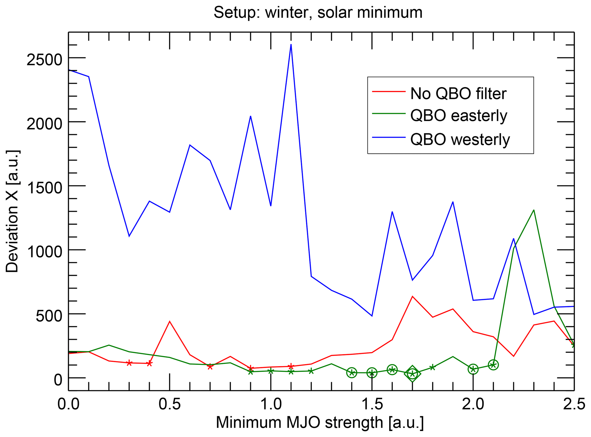
We have also checked the influence of the QBO in the context of the MJO phase evolution. For this, we excluded all epochs from the analysis, which do not match the wanted QBO phase and repeated the analysis, again resolved for different MJO strength thresholds. This has been done for boreal winter and a solar minimum epoch trigger. The results (Fig. 6) confirm a strong influence on the relationship between MJO phase evolution and solar 27-day cycle, which is consistent with the previous studies. For the QBO easterly phase, we find relatively low deviations X and significance levels between 1 % and 10 % in the center range of MJO thresholds. The deviations for QBO westerly periods are mostly more than 1 order of magnitude higher and the significance of all data points is worse than 10 %. This means that there is no significant relationship between the solar 27-day cycle and the MJO evolution based on the sawtooth-fitting approach for QBO westerly phases in contrast to QBO easterly phases. If no QBO filtering is applied, the deviations are, as expected, mostly between those of the QBO easterly and westerly filtering. Almost no data points are significant for this case.
Hence, we conclude that a possible relationship between the solar 27-day cycle and the MJO phase evolution is only detectable for QBO easterly conditions.
Note that alternatively defining the QBO phase by wind data at 30 hPa instead of 50 hPa does not qualitatively affect this conclusion (see Fig. S15 in the Supplement).
4.3.3 Seasons
It has been found before that the MJO strength modulation by both the QBO and solar influences is mostly detectable during boreal winter, i.e., the during the months December, January, and February (Yoo and Son, 2016; Hood, 2017), sometimes extended by the months March, April, and May (Hood, 2018).
We have checked the seasonality in the context of the MJO phase evolution by restricting the considered epochs to the respective months. Indeed, our results (Fig. 7) also show that a strong relation between the solar cycle and the MJO phase evolution is indicated predominantly for boreal winter. A similarly strong relation is also seen for boreal winter extended by the spring months, which we analyzed for the sake of comparability to Hood (2018). During boreal summer, some of the deviations are an order of magnitude higher and only rarely significant. Data for boreal autumn have not been computed for reasons of computation time. The unfiltered (i.e., year-round) data lead to deviations, which are mostly located between the extremes and only rarely significant.
We have to note that the findings differ in this case somewhat among the alternative numerical setups (see Sect. 4.2). In particular, that boreal winter extended by spring behaves similarly to winter only is not true for the numerical setup, in which the epoch covers −14 to 14 days around the solar extremum (see Fig. S2 in the Supplement). In this case only the boreal winter data show a clear, significant relationship, but the data extended by spring do not. Although our results appear to be largely consistent with Hood (2018), this detail is not consistent, as Hood (2018) is also based on the centered epochs.
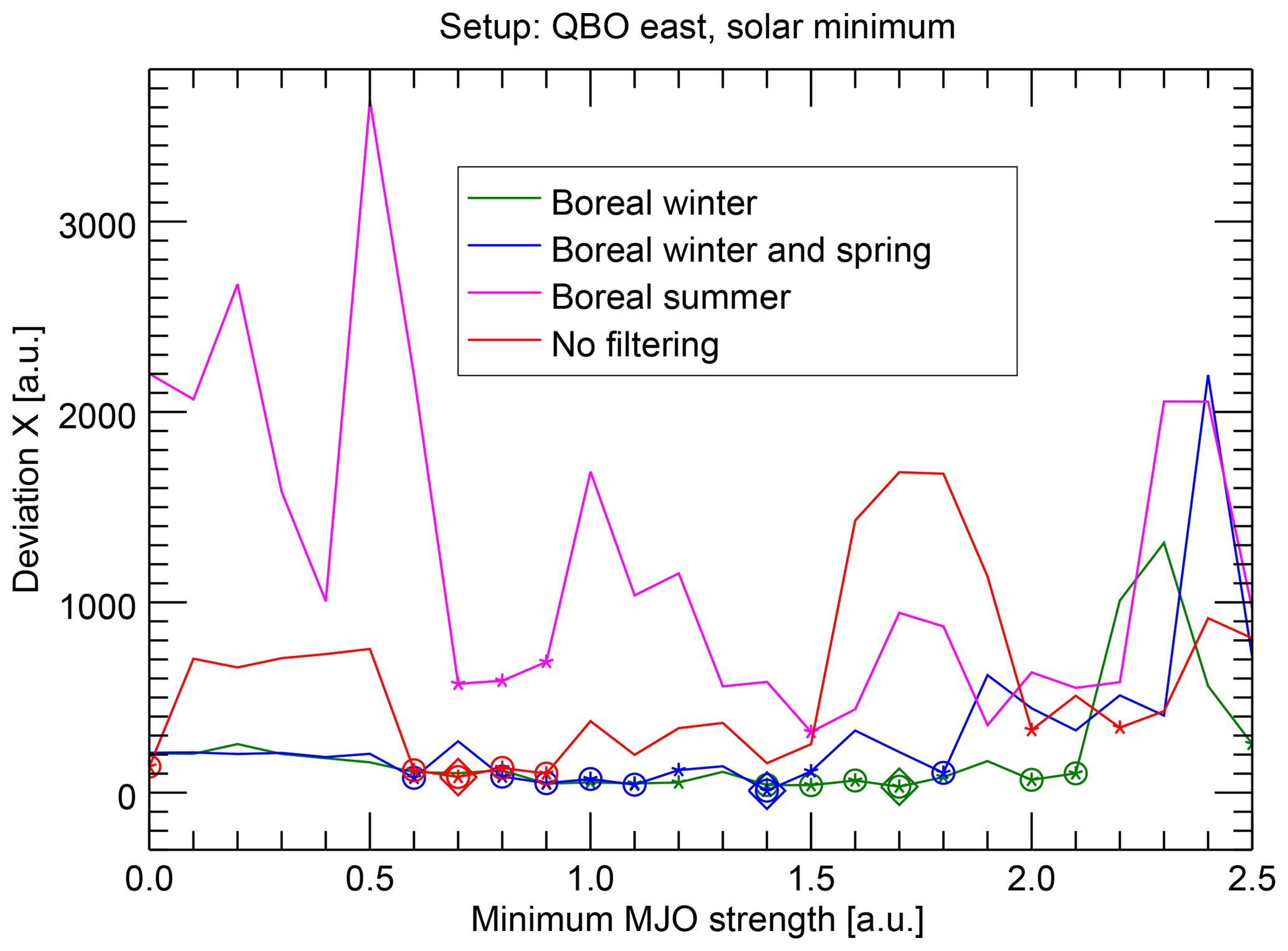
We conclude here that a possible relationship between the solar 27-day cycle and the MJO phase evolution is detectable only during boreal winter, although an extension into spring might be possible. The reasons for the seasonality are speculative, but likely connected to the reasons for the seasonality identified by Hood (2018) and maybe also to that of the QBO influence identified by Yoo and Son (2016), particularly the seasonality of the MJO itself or the seasonality of the stratospheric residual circulation.
4.3.4 Solar minimum or maximum as epoch trigger
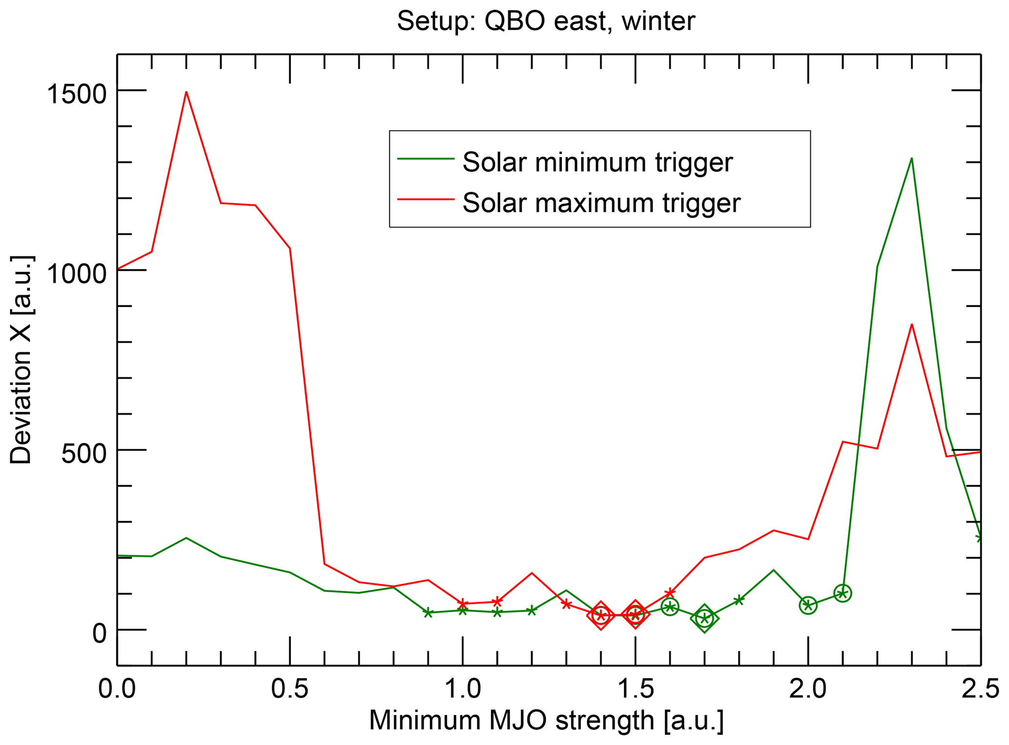
We have also checked whether it makes a difference to start the epochs with the solar 27-day minimum or maximum. It turns out that, in the reasonable range of MJO strength thresholds, the deviations X are on a similar order of magnitude for both cases (Fig. 8) and, hence, that the choice of the trigger has no pronounced effect.
Nevertheless, looking more closely, one may note that the deviations are mostly at least a bit lower and more data points are significant when the solar minimum trigger is used. These differences should not be overinterpreted, but we would like to at least mention them, because they become more pronounced when the alternative experimental setup with centered epochs is used (Fig. S3 in the Supplement). In this case, almost no data points are significant using the solar maximum trigger, whereas a continuous range over 13 data points is significant at the 5 % level for the solar minimum trigger. Overall, the influence of the trigger must therefore remain unclear in the present study. However, if a difference between both triggers could be substantiated in the future, it could hint to possible mechanisms of a synchronization between the solar 27-day cycle and the MJO; it could indicate that the solar minimum is the actual trigger, which privileges certain MJO phases and that the MJO phase evolution runs freely afterwards, so that the results are more noisy when the analysis is started half of a cycle later using the solar maximum trigger. Also the observation that the MJO is predominantly before phase 1 during solar minimum would appear consistent in this context (Sect. 4.3.1).
4.3.5 Relaxed atmospheric filter criteria
The previously presented experiments were designed such that one parameter was varied, while the other parameters were set to the optimal values. This, of course, limits the scope of the conclusions, since a clear relation between the solar 27-day cycle and the MJO phase evolution is only indicated when all conditions are met simultaneously, namely that the MJO strength threshold is in a range around 1, the QBO is in easterly phase, and the season is boreal winter. The previously shown negative results for other filter setups demonstrate that no relationship that is significant at least at the 10 % level is to be expected when one or more filter parameters are relaxed. However, as stated before, we have applied a quite conservative quantification approach in terms of the selected numerical approach (Sect 4.2) and the MC significance estimation (Sect. 4.1 and 4.5), so that it is still worth looking at an example with relaxed filter criteria to get an impression.
A second reason for looking into this example is that it overcomes one major drawback of the previous experiment design, namely that the number of samples is relatively low. Because of these low numbers one may wonder whether the relationship found is a particular feature of exactly this sample, even if this risk is actually quantified by the MC analysis. In any case, it is worthwhile to get an impression of results including more epochs.
As an example, the analysis has been repeated without the QBO and without the season constraint. The derived time lags of maximum MJO phase occurrence are shown in Fig. 9, comparably with Fig. 4. The MJO strength threshold is set to 1, as in many other studies, but the results are comparable for similar MJO thresholds. With these criteria, about 140 of possible 243 epochs are considered instead of a few tens. As expected, the deviation X is higher than in the optimally filtered case (Fig. 4) and is not considered significant anymore, with the probability to derive a lower deviation with random numbers being about 15 %. But still the data points do not appear completely disordered. Instead they still remind the eye of the sawtooth-like structure analyzed before.
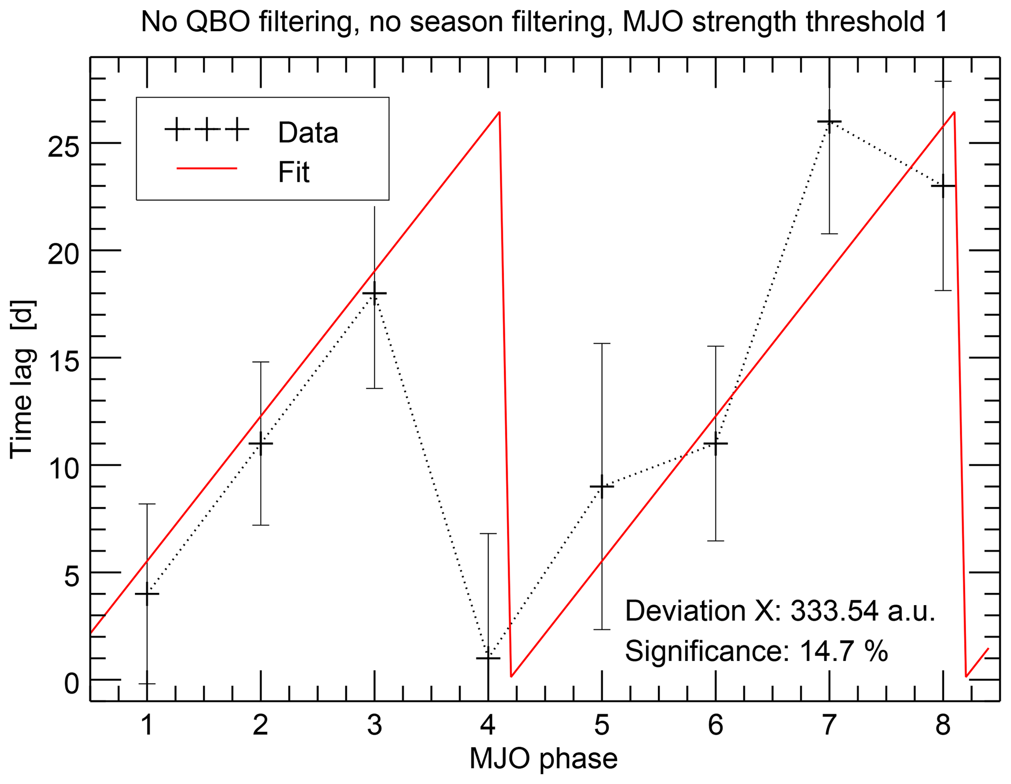
Figure 9As in Fig. 4, but showing results of an experiment without filtering for QBO phase and season. As described in the text, the results are not significant anymore on a level better than 10 %. However, it is visually seen in this figure that there are still indications for the sawtooth-like pattern instead of a totally unstructured behavior.
On the one hand, this could indicate that the described relation may also be there under different atmospheric conditions, but is superimposed by different kinds of variability. On the other hand, it may mean that the relation is so pronounced for specific atmospheric conditions that the signature remains, even when other periods are included. In conclusion, although we already analyzed 38 years of data, the period does not seem to be long enough to significantly prove a statistical connection between the solar 27-day cycle and the MJO phase evolution for more general atmospheric conditions than those described above, particularly not using our conservative MC approach. However, this does not necessarily mean that the relation is actually restricted to those conditions. Both a longer dataset and refining the analysis approach to be less conservative, of course while remaining scientifically strict, could help to answer this in the future.
Note that some more fit examples, which correspond to some cases of particularly strong deviations in the previous experiments, are shown in the Supplement. Also shown there, rudimentary indications of a sawtooth structure can sometimes still be recognized although they are highly insignificant.
4.4 Influence of underlying datasets
4.4.1 Influence of the MJO index
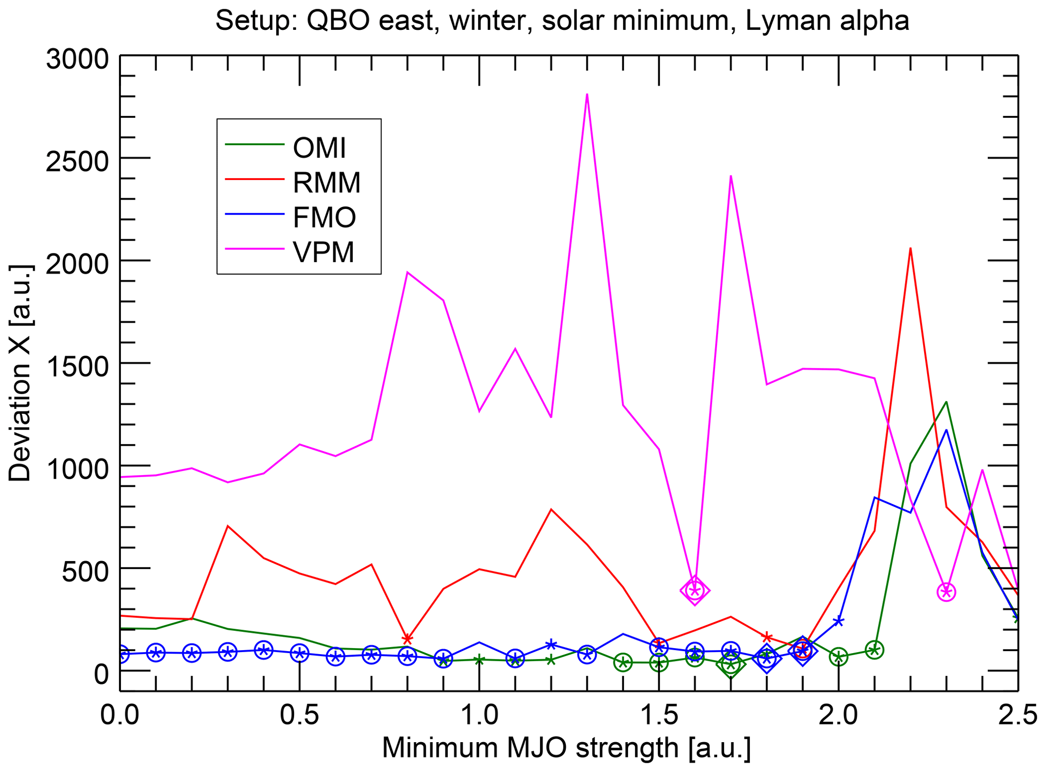
To describe the strength and phase evolution of the MJO, several independent indices have been developed in the past (Sect. 2). In addition to the analysis based on the OMI index presented before, we have repeated the analysis with other important indices, particularly the major ones discussed in Kiladis et al. (2014): RMM, VPM, and FMO.
We have recalculated, for example, the analysis described in Sect. 4.3.1, that is for the standard conditions boreal winter, QBO easterly phase, and solar minimum trigger. The results (Fig. 10) show clear differences between two pairs of the indices; while the results for OMI and FMO show relatively low deviations X, which are largely significant at the 5 % level, the other two indices RMM and VPM show much larger deviations, which are rarely significant. Hence, a relationship between the solar 27-day cycle and the MJO phase evolution is only indicated by OMI and FMO. While this result is somewhat surprising, the grouping of the indices appears plausible, since the pairs also belong together conceptually, as they are either the univariate indices OMI and FMO based only on OLR data or the multivariate indices RMM and VPM, which also include circulation data.
This can be interpreted in two ways. First, it could mean that a potential connection of solar 27-day activity is not fully represented in the circulation-based indices RMM and VPM. This appears plausible, because OMI has a more precise representation of the convective center and, hence, might better represent such subtle features we are looking for. This was exactly the reason for using OMI as the primary index as also done in, for example, Hood (2017, 2018). But second, it could mean that we did not strictly identify a connection between the solar 27-day activity and the MJO but only between the solar 27-day activity and OLR. The signature would then appear more or less accidentally in the MJO indices and we would have found a similar solar variability–OLR connection, as has been reported by Takahashi et al. (2010) using different methods. In this respect, it is appropriate to mention that Takahashi et al. (2010) and the OMI and FMO description paper by Kiladis et al. (2014) refer to the same OLR data basis, namely Liebmann and Smith (1996). If this second interpretation were true, it would mean that we have so far actually described the properties of the solar influence on OLR and not directly on the MJO. Although this was not our original objective, the results would still be interesting, as they underline the possibility of solar 27-day influences on the tropospheric parameter OLR. As in Takahashi et al. (2010), the remaining open question of interest would concern the mechanism of such a sun–OLR connection. An involvement of the MJO in such a mechanism would still be likely, as the OLR is, of course, influenced by the MJO.
Indeed, the fact that the properties of the relationship described so far are largely consistent with other MJO-related studies suggests that the MJO is at least involved in these interactions. Therefore, we propose to treat both interpretations equally seriously for the time being. To be able to distinguish both interpretations, future research should further examine the solar influence on the data ingredients of the individual MJO indices and identify processing steps in the computation of RMM and VPM, during which the solar influence could get lost.
In conclusion, although the overall picture of the present results suggests that the MJO is actually somehow involved, the present study must strictly speaking remain inconclusive regarding the question of whether the MJO is really influenced by the solar 27-day cycle or if only OLR is affected or whether the OLR signal is maybe generated by a modulation of the MJO. What can be stated, however, is that studies dealing with such subtle features of the MJO should repeat the analyses with different MJO indices and not arbitrarily select only one of them. This also concerns the aforementioned series of papers on the solar influence on the MJO, which started with the RMM index (Hood, 2016) and switched to OMI while mentioning RMM results (Hood, 2017) before relying complete on OMI (Hood, 2018). In the light of the current findings it would be of interest to know whether the results of Hood (2018) are reproducible also with RMM or not.
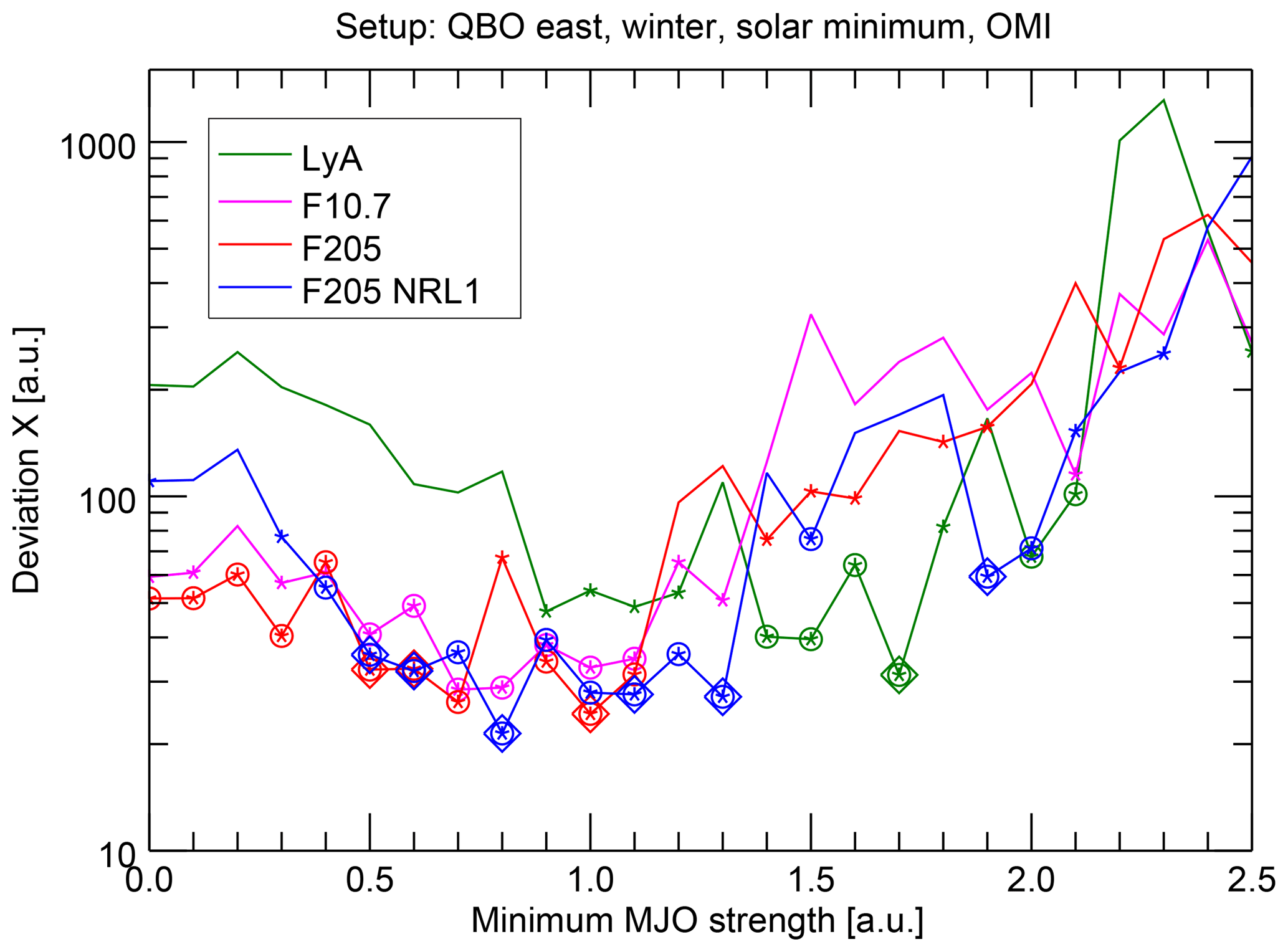
4.4.2 Influence of the solar proxy
We have also checked the influence of the solar proxy used in our study. In addition to our standard proxy Lyman alpha, we have also included the F10.7 radio flux and for comparability with Hood (2016, 2017, 2018) the UV radiation data from NRL SSI models (Sect. 2).
Generally, the solar proxy data are not as fundamental as the MJO index for our analysis, since they are only used to generate a list of dates with solar extrema, which define the epochs. The algorithm to find these local extrema in the proxy time series (Sect. 3) depends on thresholds, which are adjusted for the particular proxy. Variations in the data among the proxies and the definition of these thresholds may cause the resulting list of extrema to be a bit different depending on the proxy used. Hence the present experiment basically checks the influence of a somewhat different epoch sampling. If, hypothetically, an unambiguous list of the solar 27-day extrema had been derived, this list would be used instead of the proxy data and this kind of test would be obsolete.
As expected, the results (Fig. 11) show overall a similar shape corresponding to the description in Sect. 4.3.1, with higher deviations for low and high MJO thresholds and lower deviations in the medium range. Nevertheless, there is also considerable variability among the different curves, showing that the analysis is still sensitive to the exact sampling of the epochs, although the relatively long period of 38 years is analyzed. It appears that the range of significance is somewhat different for Lyman alpha and the alternative indices; where Lyman alpha shows significant data points between MJO strength thresholds of roughly 1 to 2, the significant range is located more between 0.3 and 1.3 for the other indices. Also, this observation should, however, not be overinterpreted, since it is not evident when using the alternative numerical setup with centered epochs (Sect. 4.2, Fig. S5 in the Supplement). In the Supplement, the significant range is more homogenous and spans a broader range from roughly 0.3 to 1.6 for most solar proxies.
The fact that the variability introduced by a somewhat different epoch sampling propagates into the final results suggests that it is currently safer to repeat such subtle analyses of the solar influence in tropospheric parameters with different proxies to check if the drawn conclusions are robust.
4.5 Significance estimation with different Monte Carlo variants
We have estimated the significance of the individual results with a MC approach as already outlined in Sect. 4.1; for each calculation result, the analysis is repeated 1000 times with randomly modified input data. The significance is then indicated by the percentage of runs, which resulted in equal or lower deviations X (stronger relationship between the solar 27-day cycle and MJO phase evolution) compared to the original calculation.
There is, however, a lot of freedom in the particular design of the random modification of the input data and, to our knowledge, there is no unambiguous argument for selecting a particular method. In contrast to this, the particular implementation is usually only briefly described in many studies and a comparison of the different results is difficult. In our case there is not only freedom in how the random component is implemented, but also to which of the three time series (MJO strength, MJO phase, list of solar extrema) it is applied. Since we are analyzing here a very subtle feature, the relationship of two quasi-periodic but still variable processes of the sun–earth system, we decided to discuss different implementations here, so that the spectrum of possible significance values becomes obvious.
The basic question for the investigation of a relationship between two quasi-periodic processes is to what extent the random modification may influence the internal temporal behavior of both processes. On the one hand, it is exactly this internal structure that characterizes the inherent nature of the processes (here, for example, the temporal evolution of the MJO) and that should not be artificially modified. On the other hand, exactly this temporal behavior has to be randomly disturbed in order to check whether the relationship of both processes reacts to this disturbance. In other words, a random modification has to be introduced, as this is the idea of the MC technique, but is has to be kept so small that the nature of the analyzed process remains comparable. This problem is also discussed in, for example, Davison and Hinkley (1997) or Chernick (2007) in the context of the bootstrap method.
Since it is mostly not obvious which idea for the random modifications meets this compromise best, we have tried different implementations, which are described in the following. The results of all implementations are compiled in Fig. 12 for the standard experiment conditions, which correspond to the example of Sect. 3: QBO easterly phase, boreal winter, MJO strength threshold 1, and solar minimum trigger. In Fig. 12, the results are ordered by a decreasing conservation of the internal structure of the original time series. In addition to the standard MJO index OMI, we have also calculated these experiments for RMM and FMO.

Figure 12Results of the different MC implementations for the standard experiment setup (QBO easterly, boreal winter, MJO strength threshold 1, and solar minimum trigger), which corresponds to the example of Sect. 3. The horizontal dashed lines mark the significance levels of 1 %, 5 %, and 10 %, respectively. The eight items are ordered according to a decreasing conservation of the internal temporal structure by the random modifications. The results are shown for the MJO indices OMI (green), FMO (blue), and RMM (red) for each implementation method. The first and the last two methods, which are separated by dashed lines, are included for completeness but do not really characterize the significance of the experiment; see Sect. 4.5 for details.
To start with one extreme, it would be possible to replace one or both time series with white noise, i.e., completely un-autocorrelated random data. It is intuitively clear that the application of the described analysis procedure to such a random time series would be very unlikely to result in a structured pattern as seen in, for example, Fig. 3. Hence, low probabilities of deriving lower deviations would be found and a high significance of the original calculation would be indicated. But looking closer, this estimation would not be very conclusive, since the characteristics of the original data, which initially motivated the analysis, are not apparent anymore in the white noise random time series. Nevertheless, we have conducted two related experiments. First, we have replaced the MJO phase time series by a time series in which the MJO phases are randomly distributed according to a uniform distribution, without any autocorrelation. Indeed, the probability to undercut the original deviation X with the random data is essentially 0 % (Fig. 12, on the very right) for OMI and FMO. The probabilities for RMM are generally higher, since the relationship was weak with this index anyway (Sect. 4.4.1). But it is, at about 1 %, still low in this case. Hence, this experiment confirms the expectation that it is unlikely to derive the sawtooth-pattern with a completely randomized MJO phase distribution. In the second approach, we have left the MJO index values untouched but have selected the dates for the solar extrema completely randomly. For this, we have selected as many out of the about 14 000 possible days as have been considered in the original analysis. Hence, the epochs are randomly distributed over the complete analyzed period and are totally independent of the actual temporal behavior of the solar proxy so that a potential temporal relation between the solar proxy and the MJO index will be broken. However, at least the temporal evolution of the MJO during the individual epochs is conserved, since the MJO index is untouched. The probability to find lower deviations with this random dataset is still below 1 % for OMI (Fig. 12, second from right), which has a somewhat stronger meaning than the first experiment; it shows that the sampling of the MJO index with epochs has to be largely systematic to reproduce the relationship found.
At the other end of the extreme, one could not touch the internal structure of all time series at all. For example, the random component could be introduced by randomly selecting subsets of the epochs originally considered, which is similar to the bootstrap method. Hence, only different subsets of the same data pairs (MJO phase and solar proxy) are evaluated and it is not very surprising that this approach results in a comparatively high probability to find similar low or lower deviations. Although we have included this result for completeness (Fig. 12, on the very left), it is not very meaningful in this context, since this experiment does not challenge the temporal relationship between both processes at all. Instead, such an analysis evaluates the influence of the particular sampling period on the result and could, for example, be used to compute error bars for the deviations (which we have not extensively done due to a limitation of computation time). Hence, this approach is not considered further on.
As a good compromise between both extremes, we ended up with shifting the originally considered solar extrema dates a bit (see also Sect. 4.1). Particularly, the extrema dates are shifted by a few days, which are randomly selected from a uniform distribution between −6 days and +6 days for each solar extremum independently. Hence, this approach modifies the temporal relation between both processes but is restrained to the effect that the evolution of the MJO is not touched at all, while the mean periodicity of the solar 27-day cycle is also conserved and only the deviations from this mean period are randomly changed. Hence, also the inherent temporal mean structure of the solar proxy is conserved when these random fluctuations are introduced. This approach leads to the already-mentioned probability of about 8 % to undercut the original deviation with the random data in the present example (Fig. 12, second from left, and Fig. 4). Considering the only slight changes of the solar extrema dates (less than 6 days compared to the large MJO period variability of a few tens of days) the 8 % appear remarkably low; i.e., the significance was remarkably high. Formulated the other way around, shifting the solar extrema dates randomly by only a few days will already weaken the relationship found between solar variability and the MJO phase evolution in 92 % of the cases. This low probability to undercut the original deviation X with this conservative approach indicates that coincidences of variations in the solar proxy and in the MJO phase time series are not very tolerant against slight temporal changes and, hence, that a synchronization of both variations might really exist. Note that for some of the previously described experiments (Sect. 4.3 and 4.4) significance values of better than 5 % and 1 % were also found using this approach.
We are not aware of any unambiguous definition of the randomly generated data but think that we have at least justified the latter approach, which has been generally used as the standard method in this study. However, we do not claim that this is the only possible approach. Aside from the fact that the range for the random shifts of ±6 days is an arbitrary definition, completely different approaches to generate the random data are conceivable. We have implemented two further ideas (with two variants each), which we will outline in the following. These approaches indicate an even higher significance of our results. However, as we are carrying out this subtle study as conservatively as possible, we have decided to use that approach as the standard, which results in the lowest significance.
Both alternatives modify the MJO time series and leave the list of solar extrema dates untouched. For the first approach the continuous MJO index time series is completely shifted by a random number of days. The shifted period can be each number of days between 0 and the length of the time series. The ending period, which exceeds the original end date of the analysis after the shift, is cut and pasted in place of the now missing starting period. To our understanding, a comparable approach has also been used in Hood (2017, 2018). For our first variant of this approach, the shift is only applied to the MJO phase evolution, whereas both phase and strength are modified similarly in the second variant. Keep in mind that phase and strength have different roles in the analysis; while the strength is only used as filter criterion, the phase is basically the analyzed quantity. This approach almost completely conserves the internal temporal structure of the MJO index except at the two seams. The only thing disturbed is the direct temporal day-to-day relation between solar variations and MJO variations. The disturbance is, however, stronger than in our standard approach, since the resulting temporal difference between originally coincident features of the solar proxy and the MJO index can be many years instead of only ±6 days. The results show (Fig. 12, third and forth item) a very low probability to undercut the original deviation, which is comparable to that of the totally random time series explained first. Hence, this approach would indicate a high significance, if treated as the deciding approach. The result of this approach further indicates that, in order to explain the observed relation, it is not enough to have two processes, which only act on related timescales in terms of the mean period. Instead, it seems that a closer temporal linkage on the basis of individual solar and MJO cycles could be necessary.
The second alternative is based on a random redistribution of individual MJO events (i.e., continuous periods starting with phase 1 and lasting until phase 1 is reached again), hence, the new MJO index time series are composed by randomly redistributing MJO event pieces of the original time series. This is also applied either to the MJO phase alone or to both phase and strength. This approach also preserves the temporal structure of the MJO to a large extent, since the mean periodicity as well as the temporal behavior of the individual MJO events are not changed. But as in the previous case, the temporal relation of the solar proxy and the MJO index is strongly disturbed, since originally coincident cycles get randomly separated by possibly long periods. The results (Fig. 12, fifth and sixth item) are comparable to those of the first alternative, which also indicates that the temporal relation between both processes on the basis of individual cycles seems to be important.
Note that also the result of the experiment with relaxed filter criteria (no filtering for QBO and season; see Sect. 4.3.5 and Fig. 9) based on OMI, which was not considered significant with 14.7 % using the standard approach, would be significant on at least a 5 % level if the latter two alternative MC approaches would be treated as decisive.
The MJO has been known to be a major source of tropospheric variability on the intraseasonal timescale for some decades. More recently, studies indicated that the solar 27-day cycle could introduce variability not only in the upper and middle atmosphere, but also in the troposphere. At first, this raises questions on how these sources can be unambiguously attributed to observed variability. But even more interestingly, there have been indications that both sources are actually linked. In particular, it has been suggested that the occurrence of strong MJO events is modulated by the solar 27-day cycle.
We have analyzed a complementary aspect, namely whether the temporal evolution of the MJO phases is potentially linked to the temporal evolution of the solar 27-day cycle. For this, we have analyzed about 38 years of MJO indices and solar proxies in combination. We have basically counted the occurrences of particular MJO phases as function of time lag after the solar 27-day extrema. To achieve comparability between different experiments, we have developed a quantification approach based on the standard least-squares fitting routine to measure the strength of such a possible relationship. We have used this to analyze the relationship under different atmospheric conditions (state of the QBO, seasons, MJO strengths), different solar cycle triggers, and different MJO indices and solar proxies. Furthermore we have applied different implementations of a MC significance analysis and compared the results.
We have indeed found indications for a synchronization between the MJO phase evolution and the solar 27-day cycle under certain conditions, which are summarized below. Overall, the relation is such that the MJO cycles through its eight phases within two solar cycles, i.e., the mean period of the MJO is twice that of the solar variation. Hence, it should be approximately 54 days, which fits well into the broad range of possible periods between 30 and 90 days known before. The phase relation between the MJO and the solar variation is such that the MJO is predominantly either between phase 8 and 1 or between phase 4 and 5 at the times of solar 27-day minimum. Consistently, the MJO transitions either from phase 2 to phase 3 or from phase 6 to phase 7 during solar maximum.
We have found that this relation is most pronounced during QBO easterly phases (defined by either 50 or 30 hPa winds) and during boreal winter, which is consistent with previous studies. The relationship can then be identified for a broad range of MJO strength thresholds between approximately 0.5 and 2.0. The upper limit is, however, probably only the artificial result of a very low number of samples and might increase with the availability of longer datasets. For these conditions combined, the relation is surprisingly clear, as shown in Fig. 3. For relaxed atmospheric filter criteria, the relation is still recognizable (e.g., Fig. 9) but is not significant anymore according to a conservative estimation. It has to be kept in mind that our selection of the 27-day extrema leads to a slight overrepresentation of solar 11-year maximum conditions in our analysis. Furthermore, interconnections between the solar 11-year state, the QBO phase, and other middle atmospheric parameters have been described in the literature before and could be relevant for the interpretation of the presented results. Unfortunately, the analyzed time series is not long enough to differentiate between 11-year maximum and minimum conditions in the present analysis.
As we have been trying to carve out a very subtle potential feature of the sun–earth system, we have implemented not only one MC experiment as significance analysis, but several variants. The basic difference among these implementations is the extent to which the random modifications may alter the original internal temporal structure of the time series. As our standard method, we have selected the most conservative one, i.e., the one which needs only modest modifications of the original time series and which has comparatively low significance values. In particular, we leave the MJO index time series as it is and randomly shift the solar extrema dates by up to ±6 days each. It is, however, difficult to find the only unambiguously correct variant for this particular problem, so that we have also discussed other implementations. With some of these variants, the relation between the solar cycle and the MJO phase evolution would actually be considered significant under more diverse conditions, including the previously mentioned relaxed atmospheric filter criteria.
Although we think that the partially surprising clarity of the results justifies already reporting on this topic now, we would like to emphasize that we do not consider the relationship to be already proven: first, not in a statistical sense, since there are many open questions left and since our analysis still suffers from a low number of samples despite the 38 analyzed years, and second, even less is clear in a causal sense, on which we have not worked so far. Even if the statistical connection is confirmed in the future, it appears difficult to undoubtedly extract the exact mechanism, which would also have to explain why the mean period of the affected process is twice that of the forcing.
One major question, which has been brought up by the present study, is why the relationship appears so clearly when using univariate OLR-based MJO indices like OMI and is almost not present when using multivariate indices like RMM. As OMI is known to better represent the convective center, one explanation could be that RMM simply fails to reproduce this subtle feature. However, another possibility, which cannot be neglected, is that the relationship is not really a property of the real MJO but only of its representation in OMI. Since OMI is only based on OLR data, this could mean that we have analyzed a relationship between the solar 27-day cycle and OLR. Despite not being our original focus, this would also be of interest, as it would be an additional indication for the presumption that upper tropospheric parameters are influenced by solar variability. And the directly following question on the mechanism of such a potential sun–OLR relationship might refer back to the MJO. In any case, the triad solar 27-day cycle, OLR, and MJO should be subject to further studies in the future.
Another major question, which could not be clearly answered by the present study, concerns the origin and the consequence of the period relation of both processes, i.e., the factor 2, which apparently connects the mean periods of the solar 27-day cycle and the MJO (54 days). This factor appears remarkable and might also support the assumption that a synchronization between the solar 27-day cycle and the MJO phase evolution really exists. However, one could also argue the other way around that this factor could be a random feature of the sun–earth system, which accidentally produces the results of the present analysis. Indeed, if one assumes that the analysis is applied to two perfect harmonic oscillations, with a factor 2 between the periods, then one would expect exactly the same sawtooth-like pattern in the results. In this case, a statistical relationship that has no causal counterpart at all would be found. However, this implicitly assumes that the phase between the two oscillations is constant, or at least that a particular phase relationship dominates during the analyzed period. This can, unfortunately, not be excluded based on the present analysis, but it appears at least questionable if such a dominant phase relation is plausible for such a variable phenomenon as the MJO without any synchronization mechanism. Hence, it was one aim of the conducted MC experiments to also quantify the influence of random variability in the context of these two quasi-periodic processes. The results of different MC implementations consistently indicated that it is not sufficient to have a constant relation of the mean periods of the two processes. Instead, the results indicated that a connection on a nearly day-to-day basis is important to reproduce such a close relationship between the processes, as seen in the real data. Nevertheless, such MC experiments might indicate that the probability for a pure coincidence of two processes with doubled periods is low, but they cannot disprove this possibility, so that this question remains open.
An additional outcome of this study is that the particular importance of the influences of the applied datasets and methods was emphasized. Studies on this topic should be repeated with different MJO indices and the precise meaning of applied MC analyses should also be discussed. In this respect, further efforts in method development would also be valuable, which could lead to a standardization of approaches to make the results more comparable. This should also include frequency analyses, which we have not applied here, but which could also help to better understand the appearance of the factor 2 between the periods of the solar 27-day cycle and the MJO phase evolution.
The source code will be made available by the authors upon request.
The datasets used in this paper are publicly accessible. The following MJO indices were obtained online from the NOAA Earth System Research Laboratory: OMI (https://www.esrl.noaa.gov/psd/mjo/mjoindex/omi.1x.txt, last access: 28 March 2019), VPM (https://www.esrl.noaa.gov/psd/mjo/mjoindex/vpm.1x.txt, last access: 28 March 2019), and FMO (https://www.esrl.noaa.gov/psd/mjo/mjoindex/fmo.1x.txt, last access: 28 March 2019). The MJO index RMM was obtained online from the Australian Bureau of Meteorology (http://www.bom.gov.au/climate/mjo/graphics/rmm.74toRealtime.txt, last access: 28 March 2019). All solar proxy time series were obtained online from the LASP Interactive Solar Irradiance Data Center (http://lasp.colorado.edu/lisird/, last access: 28 March 2019). QBO data were obtained online from the Institute for Meteorology at Freie Universität Berlin (http://www.geo.fu-berlin.de/met/ag/strat/produkte/qbo/qbo.dat, last access: 28 March 2019).
A1 Common measure for the goodness of fit χ2
Commonly, analytical functions are fitted to measured data by minimizing the quantity (e.g., Press et al., 1992). Here, the yi are the data points, wi are weights (commonly defined as with the σi being the standard deviations), is the analytical function fitted to the data points, and are the parameters, which are adjusted by the fit. The number of degrees of freedom, ν, is the number of independent data points minus the number of adjusted fit parameters. In the present case is the sawtooth function with the amplitude ASt≡27 days, the period PSt≡4 MJO phases, and the phase ϕSt, which is the only free parameter adjusted by the fit. The independent variable, x, represents the eight MJO phases, and the dependent variable, y, represents the time lags of maximum occurrence for each MJO phase.
After the fitting routine has determined the optimal parameter ϕSt, i.e., the one that leads to a minimal value of χ2, this value of χ2 summarizes the residual deviations between data and fit. Hence, it could be used as the sought measure of the deviation between the data and a sawtooth function. However, two pragmatic modifications have to be applied to derive a suitable measure in the present case, which are described in the following Sects. A2 and A3.
A2 Accounting for periodicity in the fitting process
The calculation of the individual deviations has to account for the fact that the time lags are periodic with a periodicity of 27 days. This means that, for example, the deviation between the time lags 3 and 23.5 days is not the comparatively large number of 20.5 days, but only 6.5 days, as exemplified in Fig. A1. The largest deviation that can occur is therefore days. This has to be reflected by a modified quantity measuring the deviation between data and fit, which we define as . The Δyi are initially defined to identically reproduce the original χ2, i.e, . However, after their initial calculation the values of the Δyi are restricted to the range between ±13.5 days by subtracting multiples of 27 days from the Δyi,orig, hence days, where ki counts the multiples of 27 days to be subtracted.

Figure A1Illustration of the calculation of deviations between the data points and the fitted values. For reasons of clarity, only one data point has been included (black cross). With the conventional approach, the deviation Δyorig is simply the difference between the observed and the fitted value (red cross), which is 20.5 days in this example. However, the fitted relationship is not only periodic in the direction of the abscissa, but also in the direction of the ordinate, since possible time lags repeat themselves with a period of 27 days. The observed data can therefore be virtually periodically continued and it becomes obvious that the relevant deviation Δy is that between the fitted data point and the newly introduced virtual data point (gray cross), which has a value of days (=20.5–27 days) in this example.
Instead of the minimization of χ2 commonly used for curve fitting, we use for the present study, so that the fitting routine finds the optimal fit parameter ϕSt under consideration of the periodicity of the fitted relationship.
A3 Measuring the deviation including weights
For the calculation of χ2, the individual deviations are usually weighted according to the uncertainty of the measurements yi. This is adopted here also for the calculation of . The weights wi are calculated as usual as the reciprocal variances of the measured data, i.e., with the σi being the standard deviations (the values of σi are estimated with the bootstrap method described in Sect. A4). This is, of course, a useful definition for the originally intended application of χ2 and , being the quantities to be minimized during the fitting process; the relative importance of data points with a large uncertainty is reduced and the other way around.
However, such a quantity is not suitable for the intended measure of similarity between the data points and a sawtooth function; good similarity should be indicated by a small (small deviations Δyi between data and fit). But using this kind of weighting, a comparatively small is also produced by large uncertainties, which is the opposite of the wanted behavior in this context.
A solution is to compute a different overall measure of the deviations Δyi after the fitting (which remains based on the minimization of ). A straightforward and pragmatic definition, which we introduce here as deviation X, is similar to but uses reciprocal weights: . With this definition, large uncertainties lead to a higher value of X, which indicates a weaker relation between the pattern of the data points and the sawtooth function. And the other way around, smaller uncertainties work in the same direction as small deviations between data and fit and lead to a small value of X, which indicates a stronger relation between the pattern of the data points and a sawtooth function. Hence, based on this value the relation of the solar 27-day cycle and the MJO phase evolution can be quantified and compared between different experimental setups (e.g., different filtering or underlying datasets).
We note that this definition also has disadvantages. First, it is a somewhat arbitrary choice, particularly the power of 2, with which the standard deviations σi contribute. It has been chosen analogously to the definition of χ2 but could have also been chosen differently. Second, this definition combines two factors which modify the value of X, the deviations between data and fit and the uncertainties. Hence, using this measure, it cannot be distinguished whether differences of X between experimental setups are dominated by the deviations or the uncertainties. The influence of this choice on our conclusions is discussed in Sect. 4.2 and results derived with an alternative choice are shown in the Supplement.
A4 Estimating the uncertainty of the days with maximum MJO phase occurrence
Since the derived time lags of maximum MJO phase occurrence are the result of a counting process that incorporates the complete dataset, there is no possibility to directly determine the corresponding uncertainties, i.e., the statistical distribution function and its width. A well-established approach to estimate the uncertainties for such cases is the bootstrap method (e.g., Efron, 1979; Davison and Hinkley, 1997; Chernick, 2007). Basically, random samples are drawn from the original sample to generate additional virtual samples for which the complete analysis is repeated a large number of times. This results in the distribution of possible analysis results considering random effects in the original dataset. From this distribution the uncertainty can be calculated as, for example, the standard deviation.
In our case, we use the set of identified solar extrema dates as independent members of the original sample. From these dates we draw 1000 random samples with the same number of members (sampling with replacement) and repeat the analysis for each random sample. This results in eight distribution functions of the time lags of maximum MJO phase occurrence, one for each MJO phase.
Calculating the standard deviation of these distributions as uncertainty is also somewhat more complicated than usual, again due to the periodicity of the time lags (compare Sect. A2); imagine a distribution, which is centered at time lag 26 days and symmetric with wings of a few days length on both sides. Because of the periodicity the right wing will not be located around 29 days, but at time lags around 0 to 5 days, whereas the left wing remains around 24 days. Hence, the distribution would look like a bimodal distribution with two unconnected centers. The mean value would be in the middle at about 13 days and the standard deviation would represent a width, which spans the complete range from 0 to 27 days. To overcome this problem, we shift each distribution function first, such that the maximum is located in the middle at a time lag of about 13 days, and calculate the standard deviation afterwards, which is, apart from that, not affected by the shift.
The supplement related to this article is available online at: https://doi.org/10.5194/acp-19-4235-2019-supplement.
CGH outlined the project, designed the method, performed the study and prepared the paper with substantial insight and interpretation of results provided by CvS during all previously mentioned tasks.
The authors declare that they have no conflict of interest.
We would like to thank Indrani Roy and one anonymous reviewer for their valuable comments, which helped to improve the paper significantly. This work was supported by the University of Greifswald. We acknowledge support for the article processing charge from the DFG (German Research Foundation, 393148499) and the Open Access Publication Fund of the University of Greifswald.
This paper was edited by Peter Haynes and reviewed by Indrani Roy and one anonymous referee.
Baldwin, M., Gray, L. J., Dunkerton, T. J., Hamilton, K., Haynes, P. H., Randel, W. J., Holton, J. R., Alexander, M. J., Hirota, I., Horinouchi, T., Jones, D. B. A., Kinnersley, J. S., Marquardt, C., Sato, K., and Takahashi, M.: The Quasi-biennial Oscillation, Rev. Geophys., 39, 179–229, https://doi.org/10.1029/1999RG000073, 2001. a
Chernick, M. R.: Bootstrap Methods: A Guide for Practitioners and Researchers, 2nd Edition, Wiley, Hoboken, New Jersey, USA, 2007. a, b
Coddington, O., Lean, J. L., Pilewskie, P., Snow, M., and Lindholm, D.: A Solar Irradiance Climate Data Record, B. Am. Meteorol. Soc., 97, 1265–1282, https://doi.org/10.1175/BAMS-D-14-00265.1, 2015. a, b
Damon, P. E. and Laut, P.: Pattern of Strange Errors Plagues Solar Activity and Terrestrial Climate Data, Eos Trans. Am. Geophys. Union, 85, 370–374, https://doi.org/10.1029/2004EO390005, 2011. a
Davison, A. C. and Hinkley, D. V.: Bootstrap Methods and Their Application, Cambridge Series in Statistical and Probabilistic Mathematics, Cambridge University Press, Cambridge, UK, https://doi.org/10.1017/CBO9780511802843, 1997. a, b
Efron, B.: Bootstrap Methods: Another Look at the Jackknife, Ann. Stat., 7, 1–26, https://doi.org/10.1214/aos/1176344552, 1979. a
Fytterer, T., Santee, M. L., Sinnhuber, M., and Wang, S.: The 27 Day Solar Rotational Effect on Mesospheric Nighttime OH and O3 Observations Induced by Geomagnetic Activity, J. Geophys. Res.-Space, 120, 7926–7936, https://doi.org/10.1002/2015JA021183, 2015. a
Garfinkel, C. I., Benedict, J. J., and Maloney, E. D.: Impact of the MJO on the Boreal Winter Extratropical Circulation, Geophys. Res. Lett., 41, 6055–6062, https://doi.org/10.1002/2014GL061094, 2014. a
Hong, P. K., Miyahara, H., Yokoyama, Y., Takahashi, Y., and Sato, M.: Implications for the Low Latitude Cloud Formations from Solar Activity and the Quasi-Biennial Oscillation, J. Atmos. Sol.-Terr. Phy., 73, 587–591, https://doi.org/10.1016/j.jastp.2010.11.026, 2011. a
Hood, L. L.: Coupled Stratospheric Ozone and Temperature Responses to Short-Term Changes in Solar Ultraviolet Flux: An Analysis of Nimbus 7 SBUV and SAMS Data, J. Geophys. Res.-Atmos., 91, 5264–5276, https://doi.org/10.1029/JD091iD04p05264, 1986. a, b
Hood, L. L.: Lagged Response of Tropical Tropospheric Temperature to Solar Ultraviolet Variations on Intraseasonal Time Scales, Geophys. Res. Lett., 43, 4066–4075, https://doi.org/10.1002/2016GL068855, 2016. a, b, c, d, e, f, g, h, i, j
Hood, L. L.: QBO/Solar Modulation of the Boreal Winter Madden-Julian Oscillation: A Prediction for the Coming Solar Minimum, Geophys. Res. Lett., 44, 3849–3857, https://doi.org/10.1002/2017GL072832, 2017. a, b, c, d, e, f, g, h
Hood, L. L.: Short-Term Solar Modulation of the Madden-Julian Climate Oscillation, J. Atmos. Sci., 75, 857–873, https://doi.org/10.1175/JAS-D-17-0265.1, 2018. a, b, c, d, e, f, g, h, i, j, k, l, m, n, o
Kiladis, G. N., Dias, J., Straub, K. H., Wheeler, M. C., Tulich, S. N., Kikuchi, K., Weickmann, K. M., and Ventrice, M. J.: A Comparison of OLR and Circulation-Based Indices for Tracking the MJO, Mon. Weather Rev., 142, 1697–1715, 2014. a, b, c, d, e, f, g
Köhnke, M. C., von Savigny, C., and Robert, C. E.: Observation of a 27-Day Solar Signature in Noctilucent Cloud Altitude, Adv. Space. Res., 61, 2531–2539, https://doi.org/10.1016/j.asr.2018.02.035, 2018. a
Lau, W. K.-M. and Waliser, D. E.: Intraseasonal Variability in the Atmosphere-Ocean Climate System, Springer, Berlin, Heidelberg, Germany, 2012. a
Lednyts'kyy, O., von Savigny, C., and Weber, M.: Sensitivity of Equatorial Atomic Oxygen in the MLT Region to the 11-Year and 27-Day Solar Cycles, J. Atmos. Sol.-Terr. Phy., 162, 136–150, https://doi.org/10.1016/j.jastp.2016.11.003, 2017. a
Liebmann, B. and Smith, C. A.: Description of a Complete (Interpolated) Outgoing Longwave Radiation Dataset, B. Am. Meteorol. Soc., 77, 1275–1277, 1996. a
Madden, R. A. and Julian, P. R.: Description of Global-Scale Circulation Cells in the Tropics with a 40–50 Day Period, J. Atmos. Sci., 29, 1109–1123, https://doi.org/10.1175/1520-0469(1972)029<1109:DOGSCC>2.0.CO;2, 1972. a, b
Marsh, N. D. and Svensmark, H.: Low Cloud Properties Influenced by Cosmic Rays, Phys. Rev. Lett., 85, 5004–5007, https://doi.org/10.1103/PhysRevLett.85.5004, 2000. a
Marshall, A. G., Hendon, H. H., Son, S.-W., and Lim, Y.: Impact of the Quasi-Biennial Oscillation on Predictability of the Madden–Julian Oscillation, Clim. Dynam., 49, 1365–1377, https://doi.org/10.1007/s00382-016-3392-0, 2017. a
Meehl, G. A., Arblaster, J. M., Branstator, G., and van Loon, H.: A Coupled Air–Sea Response Mechanism to Solar Forcing in the Pacific Region, J. Climate, 21, 2883–2897, https://doi.org/10.1175/2007JCLI1776.1, 2008. a
Meehl, G. A., Arblaster, J. M., Matthes, K., Sassi, F., and van Loon, H.: Amplifying the Pacific Climate System Response to a Small 11-Year Solar Cycle Forcing, Science, 325, 1114–1118, https://doi.org/10.1126/science.1172872, 2009. a
Miyahara, H., Higuchi, C., Terasawa, T., Kataoka, R., Sato, M., and Takahashi, Y.: Solar 27-day rotational period detected in wide-area lightning activity in Japan, Ann. Geophys., 35, 583–588, https://doi.org/10.5194/angeo-35-583-2017, 2017. a
Naujokat, B.: An Update of the Observed Quasi-Biennial Oscillation of the Stratospheric Winds over the Tropics, J. Atmos. Sci., 43, 1873–1877, https://doi.org/10.1175/1520-0469(1986)043<1873:AUOTOQ>2.0.CO;2, 1986. a
Press, W. H., Teukolsky, S. A., Vetterling, W. T., and Flannery, B. P.: Numerical Recipes in C (2nd Ed.): The Art of Scientific Computing, Cambridge University Press, New York, NY, USA, 1992. a
Robert, C. E., von Savigny, C., Rahpoe, N., Bovensmann, H., Burrows, J. P., DeLand, M. T., and Schwartz, M. J.: First Evidence of a 27 Day Solar Signature in Noctilucent Cloud Occurrence Frequency, J. Geophys. Res.-Atmos., 115, D00I12, https://doi.org/10.1029/2009JD012359, 2010. a, b
Son, S.-W., Lim, Y., Yoo, C., Hendon, H. H., and Kim, J.: Stratospheric Control of the Madden–Julian Oscillation, J. Climate, 30, 1909–1922, https://doi.org/10.1175/JCLI-D-16-0620.1, 2016. a
Straub, K. H.: MJO Initiation in the Real-Time Multivariate MJO Index, J. Climate, 26, 1130–1151, https://doi.org/10.1175/JCLI-D-12-00074.1, 2013. a, b
Sukhodolov, T., Rozanov, E., Ball, W. T., Peter, T., and Schmutz, W.: Modeling of the Middle Atmosphere Response to 27-Day Solar Irradiance Variability, J. Atmos. Sol.-Terr. Phy., 152–153, 50–61, https://doi.org/10.1016/j.jastp.2016.12.004, 2017. a
Svensmark, H.: Influence of Cosmic Rays on Earth's Climate, Phys. Rev. Lett., 81, 5027–5030, https://doi.org/10.1103/PhysRevLett.81.5027, 1998. a
Takahashi, Y., Okazaki, Y., Sato, M., Miyahara, H., Sakanoi, K., Hong, P. K., and Hoshino, N.: 27-day variation in cloud amount in the Western Pacific warm pool region and relationship to the solar cycle, Atmos. Chem. Phys., 10, 1577–1584, https://doi.org/10.5194/acp-10-1577-2010, 2010. a, b, c, d, e
Tapping, K. F. and Charrois, D. P.: Limits to the Accuracy of the 10.7 cm Flux, Sol. Phys., 150, 305–315, https://doi.org/10.1007/BF00712892, 1994. a
Thomas, G. E., Thurairajah, B., Hervig, M. E., von Savigny, C., and Snow, M.: Solar-Induced 27-Day Variations of Mesospheric Temperature and Water Vapor from the AIM SOFIE Experiment: Drivers of Polar Mesospheric Cloud Variability, J. Atmos. Sol.-Terr. Phy., 134, 56–68, https://doi.org/10.1016/j.jastp.2015.09.015, 2015. a, b
Thurairajah, B., Thomas, G. E., von Savigny, C., Snow, M., Hervig, M. E., Bailey, S. M., and Randall, C. E.: Solar-Induced 27-Day Variations of Polar Mesospheric Clouds from the AIM SOFIE and CIPS Experiments, J. Atmos. Sol.-Terr. Phy., 162, 122–135, https://doi.org/10.1016/j.jastp.2016.09.008, 2017. a
Tian, B., Yung, Y. L., Waliser, D. E., Tyranowski, T., Kuai, L., Fetzer, E. J., and Irion, F. W.: Intraseasonal Variations of the Tropical Total Ozone and Their Connection to the Madden-Julian Oscillation, Geophys. Res. Lett., 34, L08704, https://doi.org/10.1029/2007GL029451, 2007. a
Ventrice, M. J., Wheeler, M. C., Hendon, H. H., III, C. J. S., Thorncroft, C. D., and Kiladis, G. N.: A Modified Multivariate Madden–Julian Oscillation Index Using Velocity Potential, Mon. Weather Rev., 141, 4197–4210, 2013. a
von Savigny, C., Eichmann, K.-U., Robert, C. E., Burrows, J. P., and Weber, M.: Sensitivity of Equatorial Mesopause Temperatures to the 27-Day Solar Cycle, Geophys. Res. Lett., 39, L21804, https://doi.org/10.1029/2012GL053563, 2012. a
von Savigny, C., Peters, D. H. W., and Entzian, G.: Solar 27-day signatures in standard phase height measurements above central Europe, Atmos. Chem. Phys., 19, 2079–2093, https://doi.org/10.5194/acp-19-2079-2019, 2019. a
Wheeler, M. C. and Hendon, H. H.: An All-Season Real-Time Multivariate MJO Index: Development of an Index for Monitoring and Prediction, Mon. Weather Rev., 132, 1917–1932, https://doi.org/10.1175/1520-0493(2004)132<1917:AARMMI>2.0.CO;2, 2004. a, b
Woods, T. N., Tobiska, W. K., Rottman, G. J., and Worden, J. R.: Improved Solar Lyman α Irradiance Modeling from 1947 through 1999 Based on UARS Observations, J. Geophys. Res.-Space Phys., 105, 27195–27215, https://doi.org/10.1029/2000JA000051, 2000. a
Yang, C., Li, T., Smith, A. K., and Dou, X.: The Response of the Southern Hemisphere Middle Atmosphere to the Madden–Julian Oscillation during Austral Winter Using the Specified-Dynamics Whole Atmosphere Community Climate Model, J. Climate, 30, 8317–8333, https://doi.org/10.1175/JCLI-D-17-0063.1, 2017. a
Yoo, C. and Son, S.-W.: Modulation of the Boreal Wintertime Madden-Julian Oscillation by the Stratospheric Quasi-Biennial Oscillation, Geophys. Res. Lett., 43, 1392–1398, https://doi.org/10.1002/2016GL067762, 2016. a, b, c, d
Zhang, C.: Madden-Julian Oscillation, Rev. Geophys., 43, RG2003, https://doi.org/10.1029/2004RG000158, 2005. a, b
Zhang, C.: Madden–Julian Oscillation: Bridging Weather and Climate, B. Am. Meteorol. Soc., 94, 1849–1870, 2013. a
Zhang, Y., Liu, Y., Liu, C., and Sofieva, V. F.: Satellite Measurements of the Madden–Julian Oscillation in Wintertime Stratospheric Ozone over the Tibetan Plateau and East Asia, Adv. Atmos. Sci., 32, 1481–1492, https://doi.org/10.1007/s00376-015-5005-y, 2015. a
- Abstract
- Introduction
- Datasets and filtering
- Essential nature of the potential relation between MJO phase evolution and solar 27-day cycle
- Quantitative examination of the potential relation between MJO and solar cycle for different conditions
- Discussion and conclusions
- Code availability
- Data availability
- Appendix A: Defining a measure for the strength of a relationship between the MJO phase evolution and the solar 27-day cycle
- Author contributions
- Competing interests
- Acknowledgements
- Review statement
- References
- Supplement