the Creative Commons Attribution 4.0 License.
the Creative Commons Attribution 4.0 License.
 | 02 Apr 2019
The global climatology of the intensity of the ionospheric sporadic E layer
Bingkun Yu
Xin'an Yue
Chengyun Yang
Xiankang Dou
Baiqi Ning
Lianhuan Hu
On the basis of S4max data retrieved from COSMIC GPS radio occultation measurements, the long-term climatology of the intensity of Es layers is investigated for the period from December 2006 to January 2014. Global maps of Es intensity show the high-spatial-resolution geographical distribution and strong seasonal dependence of Es layers. The maximum intensity of Es occurs over the mid-latitudes, and its value in summer is 2–3 times larger than that in winter. A relatively strong Es layer is observed at the North Pole and South Pole, with a distinct boundary dividing the mid-latitudes and high latitudes along the 60–80∘ geomagnetic latitude band. The simulation results show that the convergence of vertical ion velocity could partially explain the seasonal dependence of Es intensity. Furthermore, some disagreements between the distributions of the calculated divergence of vertical ion velocity and the observed Es intensity indicate that other processes, such as the vertical motions of gravity waves, magnetic-field effects, meteoric mass influx into Earth's atmosphere, and the chemical processes of metallic ions, should also be considered as they may also play an important role in the spatial and seasonal variations in Es layers.


Ionospheric sporadic E (Es) layers are thin-layered structures with intense, high electron densities at 90–130 km altitudes. Rocket-borne mass-spectrometric measurements have shown that the Es layer mostly result from the ionisation of metal atoms, such as Fe+, Mg+, and Na+ (Kopp, 1997; Grebowsky and Aikin, 2002). The Es layer mainly resides over mid-latitudes and is relatively absent at the geomagnetic equator and high latitudes (Whitehead, 1989). It is widely accepted that the mechanism responsible for Es layer formation at mid-latitudes is wind shear, in which the zonal and meridional winds provide vertical wind shear convergence nodes. As a result, long-lived metallic ions are forced to converge towards the wind shear null to form a thin layer of intense metallic ionisation (Whitehead, 1961, 1970, 1989; Macleod, 1966; Nygren et al., 1984; Haldoupis, 2012). In the equatorial region, the physical process of Es irregularities is attributed to the gradient-drift instabilities associated with the equatorial electrojet (Tsunoda, 2008). At high magnetic latitudes, the vertical motion of gravity waves is very efficient in concentrating the ionisation of Es because the magnetic-field lines are nearly vertical in the polar gap (Bautista et al., 1998; MacDougall et al., 2000a, b; MacDougall and Jayachandran, 2005). The Es layer generally has a vertical scale of 1 km or less, but its horizontal scale can extend up to several hundreds of kilometres. Consequently, intense Es plasma irregularities and their sharp vertical electron density gradients seriously affect radio communications and navigation systems (Pavelyev et al., 2007). Furthermore, these effects on global positioning system (GPS) radio occultation (RO) signals detected by low-Earth-orbit (LEO) satellites can be exploited for lower-level atmospheric and ionospheric global investigations (Rocken et al., 2000; Hocke and Tsuda, 2001; Schreiner et al., 2007; Yue et al., 2010, 2011).
Observations of Es layers have been widely investigated from ground-based radars (e.g. Farley, 1985; Whitehead, 1989; Kelly, 1989; Chu and Wang, 1997; Mathews, 1998). In addition to ground-based radars, the scintillations of GPS-RO were employed to extensively investigate Es layers over the past few decades (Wu et al., 2005; Arras et al., 2008; Zeng and Sokolovskiy, 2010; Chu et al., 2011). A global map of Es layers was first presented based on a meridional chain of ionosonde stations (Leighton et al., 1962). In recent years, based on GPS-RO measurements, knowledge of the global Es layer occurrence rate (hereafter called EsOR) has been advanced remarkably. Wu et al. (2005) used phase and signal-to-noise ratio (SNR) variations from ∼6000 GPS–Challenging Minisatellite Payload (CHAMP) occultations to study the global climatology of EsOR. Arras et al. (2008) investigated the global EsOR distribution, with a resolution of , based on CHAMP, GRACE (Gravity Recovery and Climate Experiment), and COSMIC (Constellation Observing System for Meteorology, Ionosphere, and Climate) occultation data. These previous studies of global EsOR maps show a strong seasonal variation, with a summer maximum in the mid-latitudes. Chu et al. (2014) employed COSMIC measurements to study the global morphology of EsOR and the results of the theoretical simulations suggested that the EsOR seasonal variation is likely attributed to the convergence of the metallic ion flux caused by vertical wind shear. Shinagawa et al. (2017) calculated the global distribution of the vertical ion convergence and showed that local and seasonal variations in wind shear distribution could partially account for the geographical and seasonal variation in EsOR.
Many papers have reported the geographical distribution and seasonal variation in global Es layers retrieved from GPS-RO signals, and nearly all of these works focused on the EsOR. The global climatology of the intensity of Es layers has not been fully studied. The purpose of this paper is to study the global intensity of Es layers and compare the results of Es intensity with previous studies on the EsOR. The occurrence of Es layers can cause both SNR fluctuations and relative slant total electron content (TEC) peaks (Yue et al., 2015). Sometimes, the SNR has specific U-shaped structures in the amplitude of GPS-RO signals, as reported by Zeng and Sokolovskiy (2010) and Yue et al. (2015). The obvious increase in slant TEC occurring at approximately 92 km implies ionisation enhancement in Es. In this study, the scintillation index (S4 index) data, measured from SNR fluctuations in the L1 channel of the COSMIC GPS-RO profiles at altitudes between 90 and 130 km for the period from December 2006 to January 2014, are employed to study the global climatology of the ionisation of Es layers. Section 2 describes the used data sets and procedures adopted to derive the S4 index. In Sect. 3, the global long-term behaviours of Es layers with a high spatial resolution are presented and compared with the previous EsOR results, including the latitude–day, latitude–longitude, and altitude–latitude distributions; seasonal variations; and geomagnetic dependence of Es layers. In Sect. 4, on the basis of the wind shear combined with several global-scale models, namely the Whole Atmosphere Community Climate Model (WACCM) (Marsh et al., 2013), the Naval Research Laboratory (NRL) Mass Spectrometer and Incoherent Scatter (MSIS)-00 atmospheric model (Picone et al., 2002), and the International Geomagnetic Reference Field (IGRF)-12 geomagnetic-field model (Thébault et al., 2015), we calculate the global distribution of the divergence of metallic ion velocity for comparison with the observations of Es layers from COSMIC satellites. The effect of the magnetic declination angle on the divergence of the metallic ion velocity in the simulation of Es is investigated for the first time. Section 5 presents the discussion and conclusions of this paper.
The COSMIC global data sets used in this study are the COSMIC-GPS amplitude S4 indices. The GPS radio signals are received by the precise orbit determination antennas of COSMIC for each GPS-RO when a GPS sets or rises behind Earth's atmosphere, as seen by the LEO satellite. Once the GPS signal is received at the LEO satellite, the onboard algorithm of the GPS receiver measures SNR intensity fluctuations from the raw 50 Hz L1 amplitude measurements, which are then recorded in the data stream at a 1 Hz rate at the ground receiver to minimise the data record size (Syndergaard et al., 2006). The raw scintillation measurements from the receiver are therefore the root mean square (rms) of the SNR intensity fluctuation in 1 s (i.e. σI), which can be expressed as . I represents the square of the L1 SNR, and the bracket 〈〉 denotes the 1 s averaged value. The S4 indices are reconstructed by the COSMIC Data Analysis and Archive Center (CDAAC) ground processing after these σI data are downloaded (Rocken et al., 2000). During the procedure of deriving the S4 indices, two additional steps are included in the ground processing. The first step is to assume that the SNR intensity fluctuations have Gaussian distributions to calculate an approximate value of 〈I〉 from σI and 〈SNR〉. The second is to apply a low-pass filter to the time series of 〈I〉 to obtain a new average of the intensity 〈I〉new at each second to replace the 〈I〉 in the calculation of the S4 indices. After these steps, a long-term detrended S4 index can be reconstructed by CDAAC ground processing. Further details on the procedure of deriving the S4 index, along with some individual example figures, can be found in the report of Ko and Yeh (2010).
In the present study, the COSMIC global data sets specifically denote the maximum value of S4 (S4max). The COSMIC global S4max data include the S4max value and geographic latitude, longitude, altitude and local time at which S4max was detected. The computed detrended S4max index is available from 28 December 2006 onwards on the CDAAC website (http://cdaac-www.cosmic.ucar.edu/cdaac, last access: 30 December 2017). The long-term global climatology of the Es intensity is investigated based on the global S4max data from December 2006 to January 2014. Figure 1 shows the altitude distribution of the COSMIC S4max profiles. A considerable number of profiles are distributed at altitudes between 40 and 130 km, with a peak number at approximately 100 km. Information on Es layers can be extracted from amplitude fluctuations in the SNR profiles (Wu et al., 2005). Please note that as a result of the integrated influence either in the SNR or the slant TEC along the LEO-GPS ray, the effect of Es layers at high altitudes could map down to the lower tangent point altitudes, which may virtually induce multiple peaks in one RO event (Zeng and Sokolovskiy, 2010; Yue et al., 2015). In Fig. 1, the occurrence of sporadic E can be seen down to 40 km as a result of an integral problem with using RO measurements. In fact, Es layers could not be formed by the wind shear below 90 km because of the high ion-neutral collision frequencies. The Es layer over lower altitudes (between 40 and 90 km) should be some artefact resulting from the mapping effect integrated along the LEO-GPS ray. Therefore, the S4max values that appear in altitudes ranging between 90 and 130 km are used to study the Es layers in the lower ionosphere region. Figure 2 shows the entire distribution of the daily average Es intensity from 2006 to 2014 retrieved from COSMIC within latitude and longitude of one ionosonde station in Beijing (40.3∘ N, 116.2∘ E), which agrees with the ionosonde measurements (foEs). The global morphology of the Es intensity is presented, and its altitude and seasonal dependences are given at a high spatial resolution because of the large COSMIC RO data sets that have high vertical resolutions.

Figure 1The altitude distribution of COSMIC S4max profiles from December 2006 to January 2014.
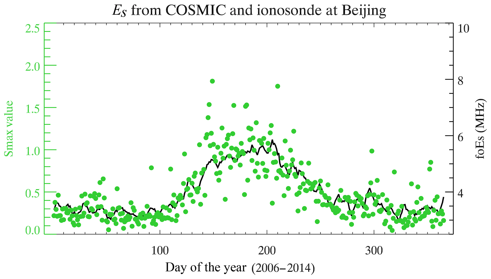
Figure 2The entire distribution of the daily average Es intensity retrieved from COSMIC within ±2.5∘ latitude and longitude of one ionosonde station and ionosonde data (foEs) in Beijing from 2006 to 2014.
Figure 3 shows the long-term time series of the Es values, with a resolution of 5∘ latitude × 5 days. As shown, the Es layer is mainly a sporadic-layered phenomenon in the summer hemisphere, as is known from former EsOR studies (Leighton et al., 1962; Wu, 2006; Arras et al., 2008; Chu et al., 2014). In Fig. 3, it is clear that the intensity of Es is enhanced in the northern (southern) summer hemisphere from May to September (from November to March), with a maximum in June (December) (i.e. 1 month ahead of the EsOR maximum, Chu et al., 2014). In addition, the seasonal Es layer also has inter-annual variability. Compared with the intense Es activity in the summers of 2010 and 2011, the intensity of Es is lower in the northern summers of 2012 and 2013, respectively. This result may be caused by anomalies in the wind field in the upper atmosphere and a corresponding reduction in the vertical wind shear associated with Es formation.
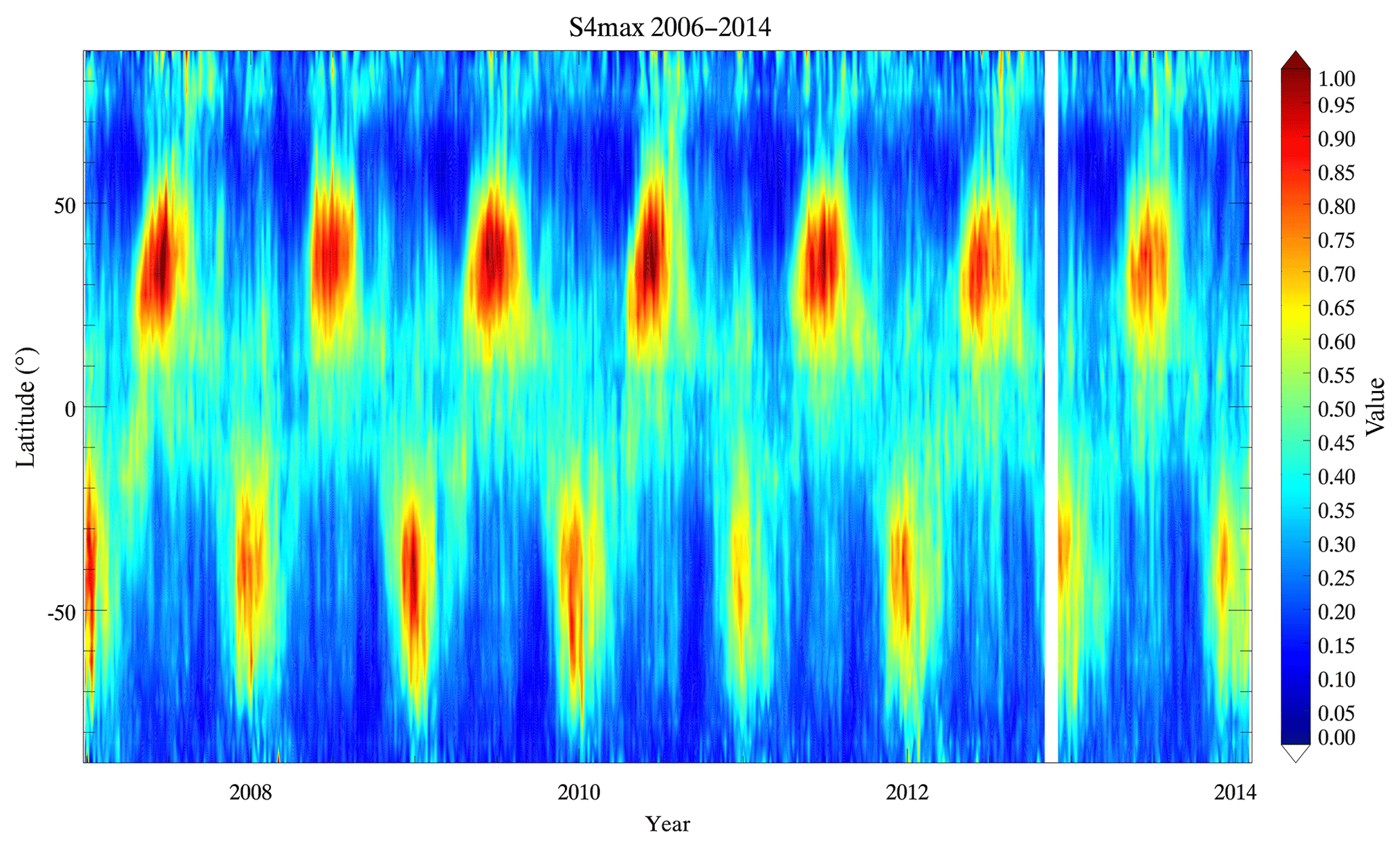
Figure 3Time series of Es intensity with a resolution of 5∘ latitude × 5 days for the period from December 2006 to January 2014.
The map in Fig. 4 shows the global geographical distributions of the Es average intensity, using a significantly improved spatial resolution of . The red and green solid curves represent the northern and southern geomagnetic latitude contours of 60, 70, and 80∘, respectively. The geomagnetic equator is also plotted with a yellow curve. The Es layers are predominantly distributed with S4max values exceeding 0.7 at mid-latitudes. Because of the increased spatial resolution, the regional features and longitudinal variations become visible. The intensity of Es is much weaker at the lower latitudes in both hemispheres, especially in the noticeable gap near the magnetic equator. When the magnetic field is horizontal at the geomagnetic equator, below the zonal wind shear action, ions move vertically due to the Lorentz force. However, they fail to converge into a layer because they are withheld by magnetised electrons. The plasma remains locally neutral. For a meridional wind shear process, ions move along the magnetic-field lines without being acted upon by Lorentz forces (Haldoupis, 2012). Therefore, a noticeable gap near the magnetic equator could be expected, which is explained by the vanishing vertical component of the geomagnetic-field lines, keeping the ionised particles from effectively vertically converging. This gap could also be found in the distribution of EsOR, although it is not as evident in Arras et al. (2008).
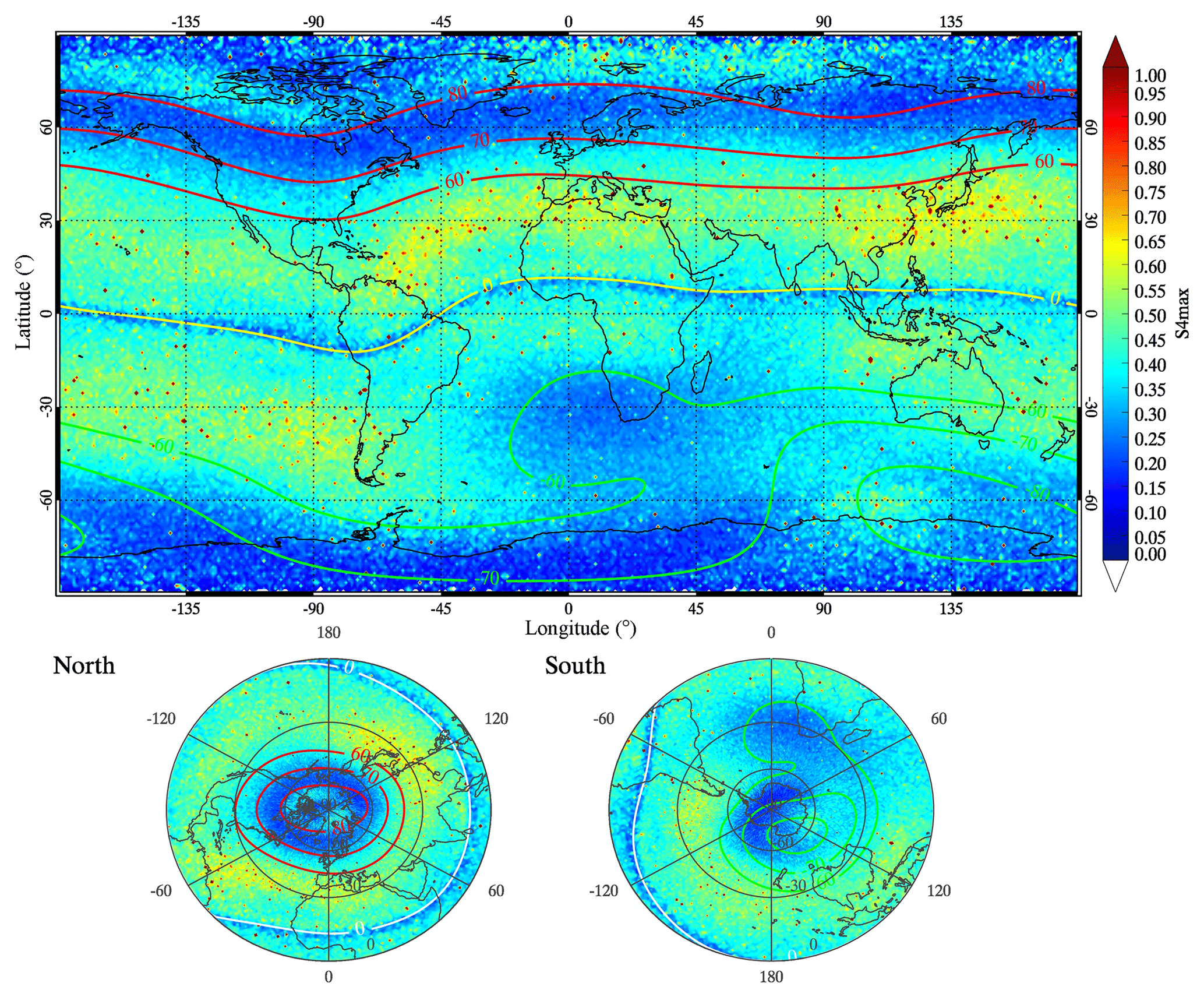
Figure 4Global geographical distributions of the Es average intensity from 2006 to 2014, with the spatial resolution of a grid. The red and green curves signify the geomagnetic latitude contours of 60, 70, and 80∘, and the yellow curve represents the geomagnetic equator.
Furthermore, the Es longitudinal variations in the geomagnetic field are also clearly shown. The decrease in Es intensity can be seen clearly in the South Atlantic Anomaly (SAA) zone and the North American region with geomagnetic latitude. The region of large Es intensity exists in the North African and North Atlantic regions, Southeast Asian region, southern African and South Pacific regions. There is a difference between the Es intensity and EsOR distributions at high latitudes: that is, the occurrence rates of Es are generally low (Arras et al., 2008), but the intensity of Es is relatively high. This pattern is more evident over the magnetic poles, which is likely the result of vertical motions of gravity waves in concentrating the ionisation of Es layers (MacDougall et al., 2000a, b). The lower panels depict the northern and southern polar views of the distributions of Es intensity, and these views make the features clearer.
The maps in Fig. 5 show the geographical distribution of Es intensity for four different seasons in a grid. The distribution of Es layers shows a significant seasonal dependence. The intensity of the Es layers in the mid-latitudes of the summer hemisphere is 2–3 times larger than that in the winter hemisphere. During spring and autumn, the intensity of the Es layers is moderate, covering the entire globe, and a distinct boundary dividing the mid-latitudes and high latitudes is visible along the 60–80∘ geomagnetic latitude band. From the polar views during each season, it can be seen that the Es layers remain at a relatively high level at the North Pole and South Pole. This characteristic could be attributed to high energy radiation, particle precipitation, and polar gap gravity waves.
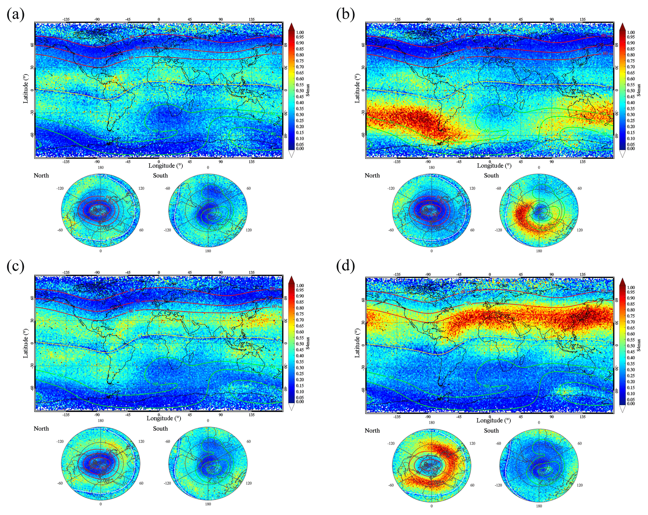
Figure 5Seasonal variations in Es intensity from 2006 to 2014, with the spatial resolution of a grid. Plots for (a) autumn (September, October, November), (b) winter (December, January, February), (c) spring (March, April, May), and (d) summer (June, July, August).
Figure 6 shows the altitude–latitude distribution of the Es intensity with a resolution of 1 km altitude latitude. The intensity of Es is distributed at altitudes between 95 and 125 km. The densest patches of Es exist at altitudes exceeding 110 km, which is different from the EsOR altitude–latitude distribution that dominates at 95–110 km, with a peak at approximately 105 km in the mid-latitudes of 25–45∘ (Arras et al., 2008). The Es intensity has a broader latitudinal extent of 10–75∘ S in the Southern Hemisphere, compared with 10–60∘ N in the Northern Hemisphere.
Figure 7 presents the seasonal variation in the altitude–latitude distributions of the Es intensity for the same temporal period and spatial resolution as those in Fig. 6. The Es intensity for the summer and winter solstices clearly has a significantly broader latitudinal extent towards the high-latitude region. In addition, the overall intensities of the Es layers increase, spanning a larger vertical extent during the solstices. In general, the Es intensity exceeding 0.65 values is distributed at altitudes of 100–125 km in the southern summer and at altitudes of 90–130 km in the northern summer. During equinox seasons, the Es intensity is moderate and its altitude–latitude distribution is relatively symmetrical.
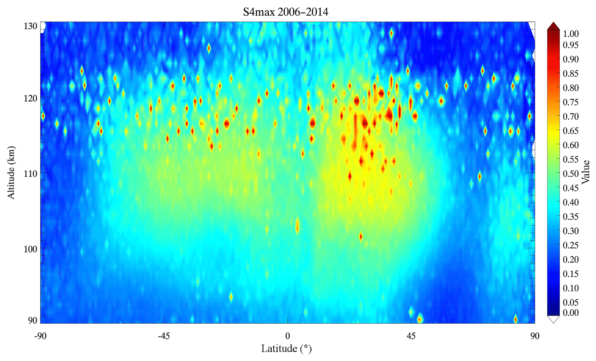
Figure 6Altitude–latitude distribution of the Es intensity from 2006 to 2014, with a resolution of 1 km altitude latitude.
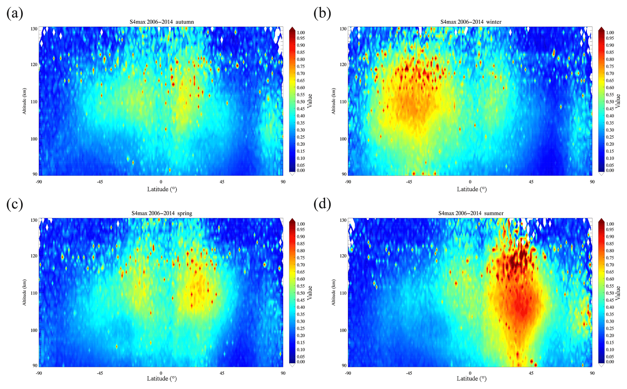
Figure 7Seasonal variations in altitude–latitude distributions of Es intensity from 2006 to 2014 for four different seasons: (a) autumn, (b) winter, (c) spring, and (d) summer.
The global climatology of the intensity of Es layers is investigated from the COSMIC occultation data, employing the GPS-RO technique. One of the pronounced variabilities in Es layers is the seasonal variation, with a maximum appearance in the summer hemisphere. Although the mechanism for Es layer formation is widely accepted, these dense and thin layers of metallic ion plasma are formed by the vertical ion convergence of neutral wind shear. The overall morphology of Es layers cannot be explained by the wind shear. One of the unsolved issues in the ionosphere is that the overall morphology, including the seasonal dependence of Es layers, does not have a comprehensive explanation (Whitehead, 1989; Haldoupis et al., 2007).
Seasonal dependence is found not only in the Es intensity but also in previous studies of EsOR variations (Wu et al., 2005; Arras et al., 2008; Chu et al., 2014). Chu et al. (2014) simulated the global distribution of the convergence of metallic ion flux caused by vertical wind shear, suggesting that the maximum Es in summer and minimum of Es in winter are likely caused by the vertical wind shear effect.
From the wind shear (e.g. Nygren et al., 1984; Mathews, 1998; Kirkwood and Nilsson, 2000), the vertical ion velocity wi induced by the neutral wind is described by Eq. (1):
where I represents the magnetic inclination angle that is defined as positive (i.e. downward direction) in the Northern Hemisphere; ri represents the ratio of the ion-neutral collision frequency (νi) to the ion gyrofrequency (ωi); and the neutral wind velocity components are in the zonal (positive for eastward), meridional (positive for northward), and vertical (positive for upward) directions. Therefore, the favourable wind field for Es layer formation is where there is a negative relationship, indicating an ion-convergence region.
Version 4 of the WACCM (WACCM4) is a global climate model with interactive chemistry, developed at the National Center for Atmospheric Research (NCAR) (Marsh et al., 2013). A specified dynamics run of WACCM4 (SD-WACCM4) was constrained by the Modern-Era Retrospective Analysis for Research and Applications (MERRA). SD-WACCM4 is used to simulate the global distribution of the divergence of ion velocity from the period of 2006 to 2014, which is consistent with the period of Es observations from the COSMIC occultation data. To compare with previous studies, the neutral wind is provided by the output from WACCM, and the ion-neutral frequency is calculated by the atmospheric composition from the MSIS-00 atmospheric model in accordance with Chu et al. (2014). The global distributions of the geomagnetic field and magnetic inclination angle at 100 km are estimated from the IGRF-12 model. The calculation of ion velocity is binned and averaged in a 1∘ latitude longitude grid at WACCM altitude levels from 0 to 130 km.
Figure 8 presents simulation results of the global distributions of the monthly mean divergence in vertical ion velocity in the altitude range between 97 and 114 km in January and July. The negative (positive) ratio represents the convergence (divergence) of ions in units of m s−1 km−1. The results show a good correlation between the simulated distributions of the monthly mean divergence of vertical ion velocity in Fig. 8 and the geographical distribution of Es intensity measured from the COSMIC GPS-RO profiles in Fig. 5. Chu et al. (2014) simulated the global distributions of the mean divergence of the Fe+ concentration flux at altitudes of 94–115 km in all four seasons. The study also showed a similar simulation result for the distributions of divergence in the Fe+ concentration flux, which is well correlated with the COSMIC-measured EsOR distribution. The simulation of the divergence of vertical ion velocity supports the wind shear of Es formation and indicates that the seasonal dependence of Es layers is likely attributed to the convergence of vertical ion velocity driven by neutral wind.
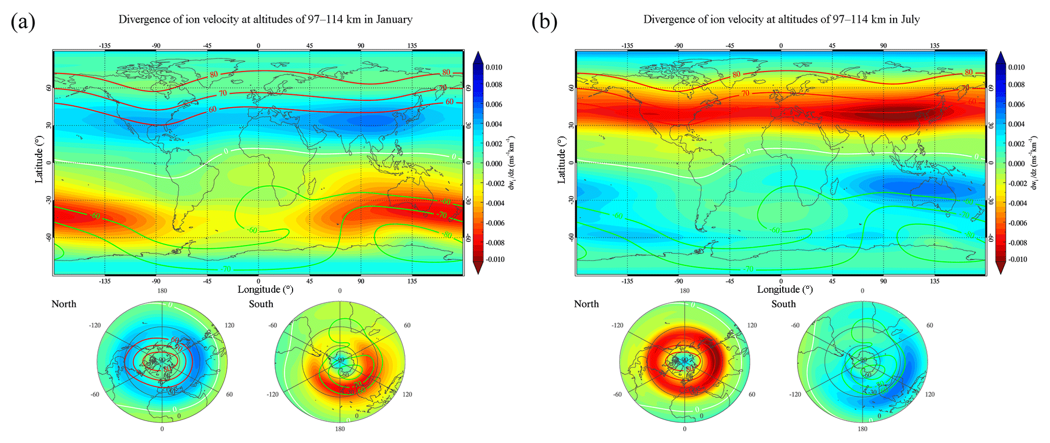
Figure 8Simulation results of the global distributions of the monthly mean divergence of vertical ion velocity from 2006 to 2014 (units of m s−1 km−1) at altitudes ranging between 97 and 114 km in January (a) and July (b). The red and green curves signify 60, 70, and 80∘ geomagnetic latitude contours, and the yellow curve represents the geomagnetic equator.
Furthermore, we also notice that the Es intensity is distributed at relatively high altitudes of 95–125 km compared with the EsOR at 90–120 km. The densest patches of Es exist above 115 km, and the Es layer has a broader vertical extent in summer, as shown in Fig. 7. In the simulation, the distributions of the monthly mean divergence of the vertical ion velocity at an altitude range of 114–128 km in January and July are shown in Fig. 9. In contrast with the distributions of the divergence of vertical ion velocity between 97 and 114 km in Fig. 8, Fig. 9 shows an ion-divergence region at altitudes of 114–128 km in summer over mid-latitudes as a result of different zonal and meridional winds. These results suggest that the wind shear alone has difficulty explaining the Es seasonal dependence at higher altitudes (114–128 km), although the wind shear is considered the primary theory for explaining the physical production of Es layers (Whitehead, 1989; Haldoupis et al., 2007).
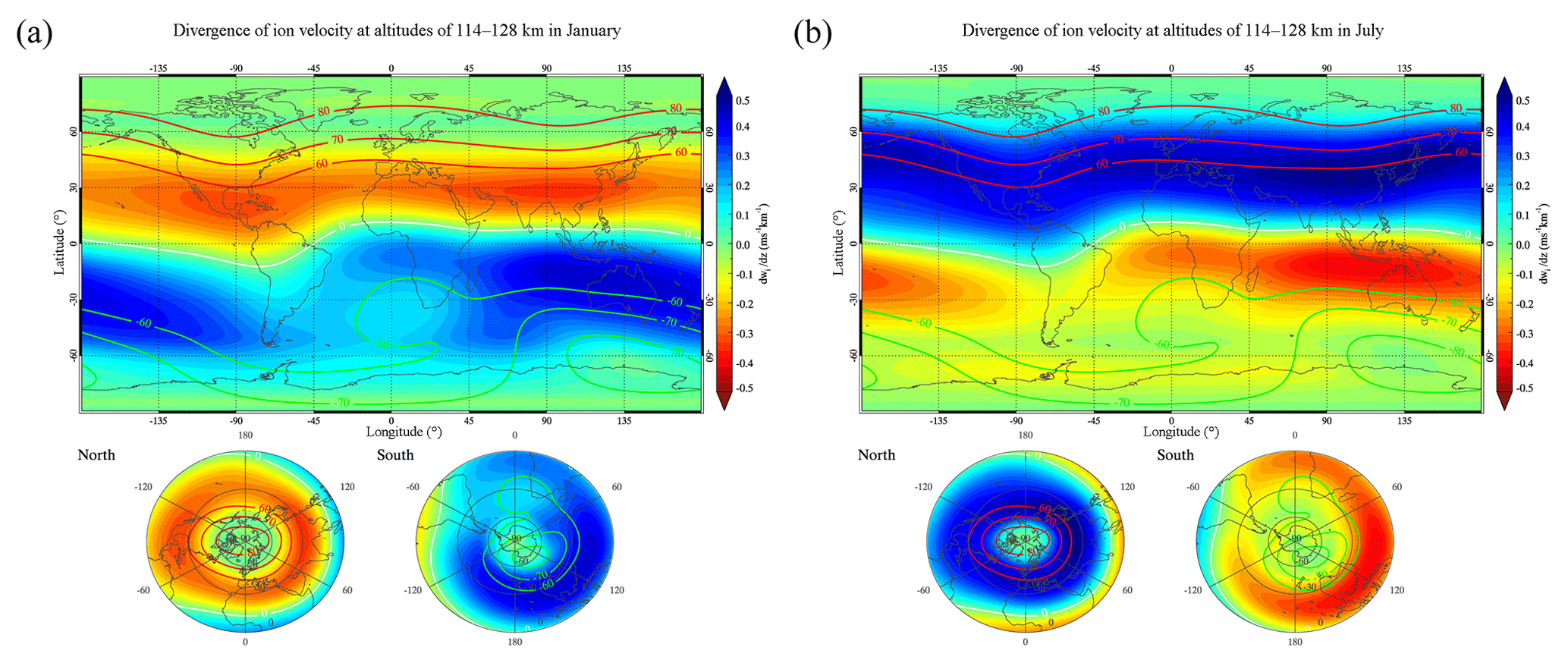
Figure 9Same as Fig. 8 but for the altitude range between 114 and 128 km in January (a) and July (b).
In previous studies on the wind shear of Es layer formation, the magnetic declination angle effect is neglected in the calculation of the vertical ion velocity wi induced by the neutral wind. The steady-state ion momentum equation is as follows:
On the basis of the steady-state ion momentum equation, the Eq. (1) for the vertical ion velocity wi is extended to take the magnetic declination angle D into consideration as follows:
The magnetic declination angle currently ranges from W to 26∘ E; therefore, it is expected to have an influence on the vertical ion velocity wi. The effect of the magnetic declination angle on the divergence in ion velocity in the simulation of Es is investigated. Figure 10 presents the global distributions of the monthly mean divergence in vertical ion velocity at altitudes ranging from 97 to 114 km with the consideration of the magnetic declination angle. The figure shows a seasonal dependence, with ion-convergence regions in summer and ion-divergence regions in winter. However, the morphology of the divergence of the vertical ion velocity is different from that without the magnetic declination angle considered in Fig. 8. In January, strong ion convergence appears in the SAA region. In July, Asia, Europe, and the North Pacific tend to be regions of ion convergence. The agreement with the observations becomes worse, which could imply that the cause of global Es layers remains a mystery because it cannot be fully accounted for by the wind shear effect (Whitehead, 1989; Haldoupis et al., 2007). The formation of mid-latitude Es layers could be partially explained by the wind shear. The investigation of the causes of seasonal variability in Es should lead to more detailed studies so that we can fully understand and properly quantify the properties of Es layers.
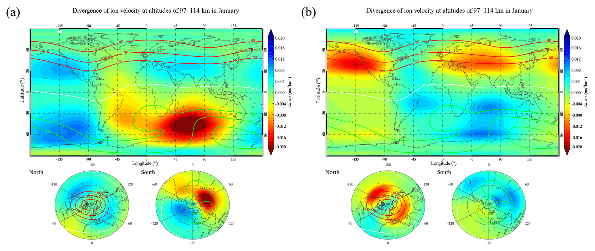
Figure 10Same as Fig. 8 but with the consideration of the effect of the magnetic declination angle on the vertical ion velocity in January (a) and July (b).
The seasonal and geographical dependences of EsOR have been widely studied by ionospheric observations since the 1960s (Leighton et al., 1962; Smith, 1978; Wu et al., 2005; Arras et al., 2008; Zeng and Sokolovskiy, 2010), but, thus far, the overall morphology of Es is still not well explained. The seasonal dependence of Es layers remains an ongoing mystery, as it is unexpected in the classical wind shear reported in the review article of Whitehead (1989). Recently, Chu et al. (2014) simulated the distribution of the convergence of the Fe+ concentration flux and indicated that the vertical ion convergence caused by neutral wind could be responsible for the seasonal dependence of Es.
In our investigations, the global climatology of the intensity of Es layers is found to also have a seasonal dependence, with a pronounced maximum over mid-latitudes in the summer hemisphere, as shown in Fig. 5. The Es intensity has similar seasonal and spatial distributions to the EsOR, but the Es layer has a relatively large intensity and a small EsOR value at the North Pole and South Pole. The wind shear mechanism does not work efficiently at either auroral zones or the magnetic equator (Haldoupis, 2012); therefore, the strong Es layers in the Earth's polar regions could be initially caused by gravity waves (Bautista et al., 1998; MacDougall et al., 2000a, b). In the simulations, the gravity waves with horizontal wavelengths smaller than ∼200 km are not explicitly resolved in WACCM (Liu et al., 2014). In particular, the vertical motion of gravity waves dominates the formation of the Es layer on the polar cap, where the near-vertical magnetic field significantly reduces the effectiveness of wind-shear in converging ions into layers. Polar-cap gravity waves have been studied by Johnson et al. (1995) and MacDougall et al. (1997). These layers are maintained in an ionised state through charge exchange of neutral metal atoms with NO+ and ions by photoionisation. These studies found that the vertical motion of gravity waves is very efficient in concentrating polar-cap Es layers. The short-lived polar-cap Es layers in winter appear to be associated with gravity waves. In summer the polar-cap Es layers are long-lasting and thin. These initial concentrations of metallic ions persist and change into long-lived Es because of ambient metallic ions produced by photoionisation in the sunlit E region (MacDougall et al., 2000a). The Es layers at the cusp latitude are relatively different from those at the polar cap. The cusp Es could be associated with the convergence of ionisation by the electric fields (MacDougall and Jayachandran, 2005).
On the other hand, simulating the global distributions of the monthly mean divergence of vertical ion velocity in an altitude range between 97 and 114 km shows an ion-convergence region in the summer mid-latitudes, which is similar to the simulation results of Chu et al. (2014). This result suggests that the seasonal dependence of Es is likely attributed to the vertical convergence of ions driven by neutral wind. However, some disagreements between the distributions of the calculated divergence of vertical ion velocity and observed Es intensity are found. For example, there are ion-divergence regions in the mid-latitudes in winter in Fig. 8, but the dissipation of Es is observed in the 60–80∘ geomagnetic latitude band. The densest Es layer appears above 115 km, which is higher than the EsOR. Another discrepancy is that the simulated divergence of vertical ion velocity in an altitude range between 114 and 128 km has a positive ratio in the summer hemisphere, which indicates an ion-divergence region of ions in contrast with the observed summer maximum of Es intensity in the summer mid-latitudes.
The effect of the magnetic declination angle on the divergence of metallic ion velocity is investigated in the simulation of Es for the first time in Fig. 10. Though the figure shows marked seasonal dependence, with a strong summer ion-convergence region, the morphology of the divergence of vertical ion velocity is different from the distribution of the observed Es intensity in Fig. 5. Thus, the vertical ion convergence by itself is far from sufficient for explaining the strong Es summer maximum. Other physical processes should also be considered in the geographical distribution and spatial variations in Es layers, as they play important roles in determining the global morphology of Es, such as the magnetic field, ionospheric electric field, the chemical processes of metallic ions, large geomagnetic storms, and meteorological processes in the lower atmosphere (e.g. Bautista et al., 1998; Mathews, 1998; Carter and Forbes, 1999; MacDougall et al., 2000a, b; Davis and Johnson, 2005; MacDougall and Jayachandran, 2005; Johnson and Davis, 2006; Haldoupis, 2012; Yue et al., 2012; Feng et al., 2013; Yu et al., 2015).
Haldoupis et al. (2007) proposed that the seasonal dependence of Es could be explained by the seasonal variation in the meteor influx into the upper atmosphere. However, it has been largely accepted that sporadic meteoroids provide a much greater meteor mass on average than meteor showers (Ceplecha et al., 1998; Baggaley, 2002; Janches et al., 2002; Williams and Murad, 2002). The meteoric mass influx caused by sporadic meteoroids reaches a maximum in autumn rather than summer (Janches et al., 2006). The global input of meteoric material is well established to enhance the mesospheric metal layers and Es layers (Plane, 2004; Plane et al., 2015). Carrillo-Sánchez et al. (2016) estimated the global interplanetary dust particles (IDPs) to be 43±14 t d−1; this was taken from three different observations in order to constrain the relative contributions of each dust source to lidar observations of the vertical Na and Fe fluxes. However, the daily amount is still not well defined. Estimates of the IDP range from 5 to 270 t d−1, depending on the different methods used to make the estimate (Plane, 2012). These effects of meteoric ablation are significantly influenced by the magnitude of the IDP input with 2 orders of magnitude uncertainty. On the other hand, this fact also highlights the importance of a fundamental understanding of the global climatology of Es layers.
In this study, we investigate the long-term climatology of the intensity of Es layers on the basis of S4max data retrieved from COSMIC GPS-RO measurements. The resulting global Es maps with a high spatial resolution present the geographical distributions and strong seasonal dependence of Es intensity, which agrees with former studies of global EsOR maps (Wu, 2006; Arras et al., 2008; Chu et al., 2014). The high Es intensity in summer exists at altitudes of 115–125 km at 10–60∘ latitude in the Northern Hemisphere and at altitudes of 115–120 km at 10–75∘ latitudes in the Southern Hemisphere.
Furthermore, the simulation results of the global distributions of the monthly mean divergence of vertical ion velocity could partially explain the seasonal dependence of Es intensity. We show that the elemental mechanism responsible for Es layers based on wind shear could explain the seasonal dependence of Es intensity (97–114 km), but it is hard to explain the Es seasonal dependence at higher altitudes (114–128 km). To further investigate the magnetic-field effects on the wind shear processes of Es formation, the effect of the magnetic declination angle on the divergence of metallic ion velocity in the simulation of Es is investigated, and we discuss some disagreements between the distributions of the calculated divergence of vertical ion velocity and the observed Es intensity. Although the wind shear of Es formation was conceived and formulated in the 1960s (Whitehead, 1961), its importance for understanding the formation of Es must have escaped attention. This study implies that, in addition to the vertical wind shear effects, other processes, such as the vertical motion of gravity waves, magnetic-field effects, meteoric mass influx into Earth's atmosphere, and the chemical processes of metallic ions, should also be considered, which could play a dominant role in the geographical and seasonal variations in Es layers. To accurately understand and properly quantify the properties of Es layers on a global scale that are also associated with the distribution of global metallic ions, we need to combine more ground-based ionosonde data with satellite observations and extensively study the geographical and seasonal variations in Es layers.
The COSMIC global data sets are downloaded from https://cdaac-www.cosmic.ucar.edu/cdaac/ (last access: 30 December 2017).
BY and XX designed the study and wrote the manuscript. XY provided the COSMIC radio occultation data and contributed significantly to the comments on an early version of the manuscript. CY and CY discussed the results of the wind shear simulation. BN and LH provided the manually scaled ionospheric observation from Beijing. XD contributed to the discussion of the results and the preparation of the manuscript. All authors discussed the results and commented on the manuscript at all stages.
The authors declare that they have no conflict of interest.
This article is part of the special issue “Layered phenomena in the mesopause region (ACP/AMT inter-journal SI)”. It is a result of the LPMR workshop 2017 (LPMR-2017), Kühlungsborn, Germany, 18–22 September 2017.
We acknowledge the COSMIC (Constellation Observing System for Meteorology, Ionosphere, and Climate) radio occultation data, the ionosonde data from the Chinese Meridian Project, the Solar-Terrestrial Environment Research Network (STERN), the Data Center for Geophysics, Data Sharing Infrastructure of Earth System Science, and the National Science & Technology Infrastructure of China, as well as the Whole Atmosphere Community Climate Model (WACCM), NRL Mass Spectrometer and Incoherent Scatter (MSIS)-00 atmospheric model, and International Geomagnetic Reference Field (IGRF)-12 geomagnetic field model data used in this paper. This work is supported by the National Natural Science Foundation of China (41774158, 41474129, 41421063,41804147), the open research project of CAS Large Research Infrastructures, the Youth Innovation Promotion Association of the Chinese Academy of Sciences (2011324), Anhui Provincial Natural Science Foundation (1908085QD155) and the Fundamental Research Fund for the Central Universities. Bingkun Yu is also supported by a Newton International Fellowship from the Royal Society.
This paper was edited by Bernd Funke and reviewed by three anonymous referees.
Arras, C., Wickert, J., Beyerle, G., Heise, S., Schmidt, T., and Jacobi, C.: A global climatology of ionospheric irregularities derived from GPS radio occultation, Geophys. Res. Lett., 35, L14809, https://doi.org/10.1029/2008GL034158, 2008. a, b, c, d, e, f, g, h, i
Baggaley, W. J.: Radar observations, Cambridge University Press, Cambridge, 2002. a
Bautista, M. A., Romano, P., and Pradhan, A. K.: Resonance-averaged photoionization cross sections for astrophysical models, Astrophys. J. Suppl. S., 118, 259–265, 1998. a, b, c
Carrillo-Sánchez, J. D., Plane, J. M. C., Feng, W., Nesvornỳ, D., and Janches, D.: On the size and velocity distribution of cosmic dust particles entering the atmosphere, Geophys. Res. Lett., 42, 6518–6525, 2015.
Carrillo-Sánchez, J. D., Nesvornỳ, D., Pokornỳ, P., Janches, D., and Plane, J. M. C.: Sources of cosmic dust in the Earth's atmosphere, Geophys. Res. Lett., 43, 11979–11986, https://doi.org/10.1002/2016GL071697, 2016. a
Carter, L. N. and Forbes, J. M.: Global transport and localized layering of metallic ions in the upper atmosphere, Ann. Geophys., 17, 190–209, 1999. a
Ceplecha, Z., Borovička, J., Elford, W. G., ReVelle, D. O., Hawkes, R. L., Porubčan, V., and Šimek, M.: Meteor phenomena and bodies, Space Sci. Rev., 84, 327–471, 1998. a
Chu, Y., Wang, C., Wu, K., Chen, K., Tzeng, K. J., Su, C., Feng, W., and Plane, J. M. C.: Morphology of sporadic E layer retrieved from COSMIC GPS radio occultation measurements: Wind shear theory examination, J. Geophys. Res.-Space, 119, 2117–2136, 2014. a, b, c, d, e, f, g, h, i, j
Chu, Y.-H. and Wang, C.-Y.: Interferometry observations of three-dimensional spatial structures of sporadic E irregularities using the Chung-Li VHF radar, Radio Sci., 32, 817–832, 1997. a
Chu, Y.-H., Brahmanandam, P. S., Wang, C.-Y., Su, C.-L., and Kuong, R.-M.: Coordinated sporadic E layer observations made with Chung-Li 30 MHz radar, ionosonde and FORMOSAT-3/COSMIC satellites, J. Atmos. Sol.-Terr. Phy., 73, 883–894, 2011. a
Davis, C. J. and Johnson, C. G.: Lightning-induced intensification of the ionospheric sporadic E layer, Nature, 435, 799–801, https://doi.org/10.1038/nature03638, 2005. a
Farley, D. T.: Theory of equatorial electrojet plasma waves-new developments and current status, J. Atmos. Terr. Phys., 47, 729–744, 1985. a
Feng, W., Marsh, D. R., Chipperfield, M. P., Janches, D., Höffner, J., Yi, F., and Plane, J. M. C.: A global atmospheric model of meteoric iron, J. Geophys. Res.-Atmos., 118, 9456–9474, 2013. a
Grebowsky, J. M. and Aikin, A.: In situ measurements of meteoric ions, in: Meteors in the Earth's Atmosphere, edited by: Murad, E. and Williams, I. P., 189–214, Cambridge Univ. Press, UK, 2002. a
Haldoupis, C.: Midlatitude sporadic E. A typical paradigm of atmosphere-ionosphere coupling, Space Sci. Rev., 168, 441–461, 2012. a, b, c, d
Haldoupis, C., Pancheva, D., Singer, W., Meek, C., and MacDougall, J.: An explanation for the seasonal dependence of midlatitude sporadic E layers, J. Geophys. Res.-Space, 112, A06315, https://doi.org/10.1029/2007JA012322, 2007. a, b, c, d
Hocke, K. and Tsuda, T.: Gravity waves and ionospheric irregularities over tropical convection zones observed by GPS/MET radio occultation, Geophys. Res. Lett., 28, 2815–2818, 2001. a
Janches, D., Pellinen-Wannberg, A., Wannberg, G., Westman, A., Häggström, I., and Meisel, D. D.: Tristatic observations of meteors using the 930 MHz European Incoherent Scatter radar system, J. Geophys. Res.-Space, 107, 14–1, https://doi.org/10.1029/2001JA009205, 2002. a
Janches, D., Heinselman, C. J., Chau, J. L., Chandran, A., and Woodman, R.: Modeling the global micrometeor input function in the upper atmosphere observed by high power and large aperture radars, J. Geophys. Res.-Space, 111, A07317, https://doi.org/10.1029/2006JA011628, 2006. a
Johnson, C. G. and Davis, C. J.: The location of lightning affecting the ionospheric sporadic-E layer as evidence for multiple enhancement mechanisms, Geophys. Res. Lett., 33, L07811, https://doi.org/10.1029/2005GL025294, 2006. a
Johnson, F. S., Hanson, W. B., Hodges, R. R., Coley, W. R., Carignan, G. R., and Spencer, N. W.: Gravity waves near 300 km over the polar caps, J. Geophys. Res.-Space, 100, 23993–24002, 1995. a
Kelley, M. C.: The Earth's Ionosphere, Int. Geophys. Ser., 43, 71, Academic, San Diego, Calif., 1989. a
Kirkwood, S. and Nilsson, H.: High-latitude sporadic-E and other thin layers–the role of magnetospheric electric fields, Space Sci. Rev., 91, 579–613, 2000. a
Ko, C. P. and Yeh, H. C.: COSMIC/FORMOSAT-3 observations of equatorial F region irregularities in the SAA longitude sector, J. Geophys. Res.-Space, 115, A11309, https://doi.org/10.1029/2010JA015618, 2010. a
Kopp, E.: On the abundance of metal ions in the lower ionosphere, J. Geophys. Res.-Space, 102, 9667–9674, 1997. a
Leighton, H. I., Shapley, A. H., and Smith, E. K.: The occurrence of sporadic E during IGY, in: Ionospheric Sporadic E, Int. Ser. Monogr. Electromagn. Waves, vol. 2, pp. 166–177, Pergamon, Oxford, UK, 1962. a, b, c
Liu, H.-L., McInerney, J. M., Santos, S., Lauritzen, P. H., Taylor, M. A., and Pedatella, N. M.: Gravity waves simulated by high-resolution whole atmosphere community climate model, Geophys. Res. Lett., 41, 9106–9112, 2014. a
MacDougall, J. W. and Jayachandran, P. T.: Sporadic E at cusp latitudes, J. Atmos. Sol.-Terr. Phy., 67, 1419–1426, 2005. a, b, c
MacDougall, J. W., Hall, G. E., and Hayashi, K.: F region gravity waves in the central polar cap, J. Geophys. Res.-Space, 102, 14513–14530, 1997. a
MacDougall, J. W., Jayachandran, P. T., and Plane, J. M. C.: Polar cap Sporadic-E: part 1, observations, J. Atmos. Sol.-Terr. Phy., 62, 1155–1167, 2000a. a, b, c, d, e
MacDougall, J. W., Plane, J. M. C., and Jayachandran, P. T.: Polar cap Sporadic-E: part 2, modeling, J. Atmos. Sol.-Terr. Phy., 62, 1169–1176, 2000b. a, b, c, d
Macleod, M. A.: Sporadic E theory. I. Collision-geomagnetic equilibrium, J. Atmos. Sci., 23, 96–109, 1966. a
Marsh, D. R., Mills, M. J., Kinnison, D. E., Lamarque, J.-F., Calvo, N., and Polvani, L. M.: Climate change from 1850 to 2005 simulated in CESM1 (WACCM), J. Climate, 26, 7372–7391, 2013. a, b
Mathews, J. D.: Sporadic E: current views and recent progress, J. Atmos. Sol.-Terr. Phy., 60, 413–435, 1998. a, b, c
Nygren, T., Jalonen, L., Oksman, J., and Turunen, T.: The role of electric field and neutral wind direction in the formation of sporadic E-layers, J. Atmos. Terr. Phys., 46, 373–381, 1984. a, b
Pavelyev, A. G., Liou, Y. A., Wickert, J., Schmidt, T., Pavelyev, A. A., and Liu, S.-F.: Effects of the ionosphere and solar activity on radio occultation signals: Application to CHAllenging Minisatellite Payload satellite observations, J. Geophys. Res.-Space, 112, A06326, https://doi.org/10.1029/ 2006JA011625, 2007. a
Picone, J. M., Hedin, A. E., Drob, D. P., and Aikin, A. C.: NRLMSISE-00 empirical model of the atmosphere: Statistical comparisons and scientific issues, J. Geophys. Res.-Space, 107, 1468, https://doi.org/10.1029/2002JA009430, 2002. a
Plane, J. M. C.: A time-resolved model of the mesospheric Na layer: constraints on the meteor input function, Atmos. Chem. Phys., 4, 627–638, https://doi.org/10.5194/acp-4-627-2004, 2004. a
Plane, J. M. C.: Cosmic dust in the Earth's atmosphere, Chem. Soc. Rev., 41, 6507–6518, 2012. a
Plane, J. M. C., Feng, W., and Dawkins, E. C. M. D.: The mesosphere and metals: Chemistry and changes, Chem. Rev., 115, 4497–4541, 2015. a
Rocken, C., Ying-Hwa, K., Schreiner, W. S., Hunt, D., Sokolovskiy, S., and McCormick, C.: COSMIC system description, Terr. Atmos. Ocean. Sci., 11, 21–52, 2000. a, b
Schreiner, W., Rocken, C., Sokolovskiy, S., Syndergaard, S., and Hunt, D.: Estimates of the precision of GPS radio occultations from the COSMIC/FORMOSAT-3 mission, Geophys. Res. Lett., 34, L04808, https://doi.org/10.1029/2006GL027557, 2007. a
Shinagawa, H., Miyoshi, Y., Jin, H., and Fujiwara, H.: Global distribution of neutral wind shear associated with sporadic E layers derived from GAIA, J. Geophys. Res.-Space, 122, 4450–4465, 2017. a
Smith, E. K.: Temperate zone sporadic-E maps (f0Es >7 MHz), Radio Sci., 13, 571–575, 1978. a
Syndergaard, S., Schreiner, W. S., Rocken, C., Hunt, D. C., and Dymond, K. F.: Preparing for COSMIC: Inversion and analysis of ionospheric data products, in: Atmosphere and Climate, edited by: Foelsche, U., Kirchengast, G., and Steiner, A. K., 137–146, Springer, Berlin, 2006. a
Thébault, E., Finlay, C. C., Beggan, C. D., et al.: International geomagnetic reference field: the 12th generation, Earth Planets Space, 67, 79, https://doi.org/10.1186/s40623-015-0228-9, 2015. a
Tsunoda, R. T.: On blanketing sporadic E and polarization effects near the equatorial electrojet, J. Geophys. Res.-Space, 113, A09304, https://doi.org/10.1029/2008JA013158, 2008. a
Whitehead, J. D.: The formation of the sporadic-E layer in the temperate zones, J. Atmos. Terr. Phys., 20, 49–58, 1961. a, b
Whitehead, J. D.: Production and prediction of sporadic E, Rev. Geophys., 8, 65–144, 1970. a
Whitehead, J. D.: Recent work on mid-latitude and equatorial sporadic-E, J. Atmos. Terr. Phys., 51, 401–424, 1989. a, b, c, d, e, f, g
Williams, I. P. and Murad, E.: Meteors in the Earth's Atmosphere, Cambridge University Press, Cambridge, 2002. a
Wu, D. L.: Small-scale fluctuations and scintillations in high-resolution GPS/CHAMP SNR and phase data, J. Atmos. Sol.-Terr. Phy., 68, 999–1017, 2006. a, b
Wu, D. L., Ao, C. O., Hajj, G. A., de La Torre Juarez, M., and Mannucci, A. J.: Sporadic E morphology from GPS-CHAMP radio occultation, J. Geophys. Res.-Space, 110, A01306, https://doi.org/10.1029/2004JA010701, 2005. a, b, c, d, e
Yu, B., Xue, X., Lu, G., Ma, M., Dou, X., Qie, X., Ning, B., Hu, L., Wu, J., and Chi, Y.: Evidence for lightning-associated enhancement of the ionospheric sporadic E layer dependent on lightning stroke energy, J. Geophys. Res.-Space, 120, 9202–9212, 2015. a
Yue, J., Wang, W., Richmond, A. D., and Liu, H.-L.: Quasi-two-day wave coupling of the mesosphere and lower thermosphere-ionosphere in the TIME-GCM: Two-day oscillations in the ionosphere, J. Geophys. Res.-Space, 117, A07305, https://doi.org/10.1029/2012JA017815, 2012. a
Yue, X., Schreiner, W. S., Lei, J., Rocken, C., Hunt, D. C., Kuo, Y.-H., and Wan, W.: Global ionospheric response observed by COSMIC satellites during the January 2009 stratospheric sudden warming event, J. Geophys. Res.-Space, 115, A00G09, https://doi.org/10.1029/2010JA015466, 2010. a
Yue, X., Schreiner, W. S., Hunt, D. C., Rocken, C., and Kuo, Y.-H.: Quantitative evaluation of the low Earth orbit satellite based slant total electron content determination, Adv. Space Res., 9, S09001, https://doi.org/10.1029/2011SW000687, 2011. a
Yue, X., Schreiner, W. S., Zeng, Z., Kuo, Y.-H., and Xue, X.: Case study on complex sporadic E layers observed by GPS radio occultations, Atmos. Meas. Tech., 8, 225–236, https://doi.org/10.5194/amt-8-225-2015, 2015. a, b, c
Zeng, Z. and Sokolovskiy, S.: Effect of sporadic E clouds on GPS radio occultation signals, Geophys. Res. Lett., 37, L18817, https://doi.org/10.1029/2010GL044561, 2010. a, b, c, d