the Creative Commons Attribution 4.0 License.
the Creative Commons Attribution 4.0 License.
 | 29 Mar 2019
The role of chlorine in global tropospheric chemistry
Daniel J. Jacob
Sebastian D. Eastham
Melissa P. Sulprizio
Qianjie Chen
Becky Alexander
Tomás Sherwen
Mathew J. Evans
Ben H. Lee
Jessica D. Haskins
Felipe D. Lopez-Hilfiker
Joel A. Thornton
Gregory L. Huey
Hong Liao
We present a comprehensive simulation of tropospheric chlorine within the GEOS-Chem global 3-D model of oxidant–aerosol–halogen atmospheric chemistry. The simulation includes explicit accounting of chloride mobilization from sea salt aerosol by acid displacement of HCl and by other heterogeneous processes. Additional small sources of tropospheric chlorine (combustion, organochlorines, transport from stratosphere) are also included. Reactive gas-phase chlorine Cl*, including Cl, ClO, Cl2, BrCl, ICl, HOCl, ClNO3, ClNO2, and minor species, is produced by the HCl+OH reaction and by heterogeneous conversion of sea salt aerosol chloride to BrCl, ClNO2, Cl2, and ICl. The model successfully simulates the observed mixing ratios of HCl in marine air (highest at northern midlatitudes) and the associated HNO3 decrease from acid displacement. It captures the high ClNO2 mixing ratios observed in continental surface air at night and attributes the chlorine to HCl volatilized from sea salt aerosol and transported inland following uptake by fine aerosol. The model successfully simulates the vertical profiles of HCl measured from aircraft, where enhancements in the continental boundary layer can again be largely explained by transport inland of the marine source. It does not reproduce the boundary layer Cl2 mixing ratios measured in the WINTER aircraft campaign (1–5 ppt in the daytime, low at night); the model is too high at night, which could be due to uncertainty in the rate of the reaction, but we have no explanation for the high observed Cl2 in daytime. The global mean tropospheric concentration of Cl atoms in the model is 620 cm−3 and contributes 1.0 % of the global oxidation of methane, 20 % of ethane, 14 % of propane, and 4 % of methanol. Chlorine chemistry increases global mean tropospheric BrO by 85 %, mainly through the reaction, and decreases global burdens of tropospheric ozone by 7 % and OH by 3 % through the associated bromine radical chemistry. ClNO2 chemistry drives increases in ozone of up to 8 ppb over polluted continents in winter.
- Article
(6077 KB) -
Supplement
(388 KB) - BibTeX
- EndNote


Mobilization of chloride (Cl−) from sea salt aerosol (SSA) is a large source of chlorine gases to the troposphere (Graedel and Keene, 1995; Finlayson-Pitts, 2003). These gases may generate chlorine radicals with a broad range of implications for tropospheric chemistry including the budgets of ozone, OH (the main tropospheric oxidant), volatile organic compounds (VOCs), nitrogen oxides, other halogens, and mercury (Saiz-Lopez and von Glasow, 2012; Simpson et al., 2015). Only a few global models have attempted to examine the implications of tropospheric chlorine chemistry on a global scale (Singh and Kasting, 1988; Long et al., 2014; Hossaini et al., 2016). Here we present a more comprehensive analysis of this chemistry within the framework of the GEOS-Chem chemical transport model (CTM).
Saiz-Lopez and von Glasow (2012) and Simpson et al. (2015) present recent reviews of tropospheric halogen chemistry including chlorine. Sea salt aerosols represent a large chloride flux to the atmosphere but most of that chloride is removed rapidly by deposition. Only a small fraction is mobilized to the gas phase as HCl or other species. Additional minor sources of tropospheric chlorine include open fires, coal combustion, waste incineration, industry, road salt application, fugitive dust, and ocean emission of organochlorine compounds (Lobert et al., 1999; McCulloch et al., 1999; Sarwar et al., 2012; WMO, 2014; Kolesar et al., 2018). It is useful to define Cly as total gas-phase inorganic chlorine, excluding particle-phase Cl−. Most of this Cly is present as HCl, which is removed rapidly by deposition but also serves as a source of chlorine radicals. Rapid cycling takes place between the chlorine radicals and other chlorine gases, eventually returning to HCl. Thus it is useful to define reactive chlorine Cl* as the ensemble of Cly gases other than HCl.
Cycling of chlorine affects tropospheric chemistry in a number of ways (Finlayson-Pitts, 2003; Saiz-Lopez and von Glasow, 2012). Acid displacement of Cl− by nitric acid (HNO3) is a source of aerosol (Massucci et al., 1999). Cl atoms provide a sink for methane, other VOCs (Atkinson, 1997), dimethyl sulfide (DMS) (Hoffmann et al., 2016; Chen et al., 2017), and mercury (Horowitz et al., 2017). Cycling between Cl radicals and their reservoirs drives catalytic ozone loss and converts nitrogen oxide radicals () to HNO3, decreasing both ozone and OH. Conversely, aqueous-phase reaction of Cl− with N2O5 in polluted environments produces ClNO2 radicals that photolyze in the daytime to return Cl atoms and NO2, stimulating ozone production (Behnke et al., 1997; Osthoff et al., 2008). Chlorine also interacts with other halogens (bromine, iodine), initiating further radical chemistry that affects ozone, OH, and mercury.
A number of global modeling studies have investigated tropospheric halogen chemistry but most have focused on bromine and iodine, which are more active than chlorine because of the lower chemical stability of HBr and HI (Yang et al., 2005; Saiz-Lopez et al., 2014). Interest in global modeling of tropospheric chlorine has focused principally on quantifying the Cl atom concentration as a sink for methane (Keene et al., 1990; Singh et al., 1996). Previous global 3-D models found mean tropospheric Cl atom concentrations of the order of 103 cm−3, with values up to 104 cm−3 in the marine boundary layer (MBL), and contributing 2 %–3 % of atmospheric methane oxidation (Long et al., 2014; Hossaini et al., 2016; Sherwen et al., 2016b; Schmidt et al., 2016). A regional modeling study by Sarwar et al. (2014) included ClNO2 chemistry in a standard ozone mechanism and found increases in surface ozone mixing ratios over the US of up to 7 ppb (ppb ≡ nmol mol−1).
Here we present a more comprehensive analysis of global tropospheric chlorine chemistry and its implications, building on previous model development of oxidant–aerosol–halogen chemistry in GEOS-Chem. A first capability for modeling tropospheric bromine in GEOS-Chem was introduced by Parrella et al. (2012). Eastham et al. (2014) extended it to describe stratospheric halogen chemistry including chlorine and bromine cycles. Schmidt et al. (2016) updated the tropospheric bromine simulation to include a broader suite of heterogeneous processes and extended the Eastham et al. (2014) stratospheric chlorine scheme to the troposphere. Sherwen et al. (2016a, b) added iodine chemistry and made further updates to achieve a consistent representation of tropospheric chlorine–bromine–iodine chemistry in GEOS-Chem. Chen et al. (2017) added the aqueous-phase oxidation of SO2 by HOBr and found a large effect on the MBL bromine budget. Our work advances the treatment of tropospheric chlorine in GEOS-Chem to include, in particular, a consistent treatment of SSA chloride and chlorine gases, SSA acid displacement thermodynamics, improved representation of heterogeneous chemistry, and better accounting of chlorine sources. We evaluate the model with a range of global observations for chlorine and related species. From there we quantify the global tropospheric chlorine budgets, describe the principal chemical pathways, and explore the impacts on tropospheric chemistry.
2.1 GEOS-Chem model with halogen chemistry
We build our new tropospheric chlorine simulation capability onto the standard version 11-02d of GEOS-Chem (http://www.geos-chem.org, last access: 1 March 2019). The standard version includes a detailed tropospheric oxidant–aerosol–halogen mechanism as described by Sherwen et al. (2016b) and Chen et al. (2017). It includes 12 gas-phase Cly species: Cl, Cl2, Cl2O2, ClNO2, ClNO3, ClO, ClOO, OClO, BrCl, ICl, HOCl, and HCl. It allows for heterogeneous chemistry initiated by SSA Cl− but does not actually track the SSA Cl− concentration and its exchange with gas-phase Cly. Here we add two new transported reactive species to GEOS-Chem to describe Cl− aerosol, one for the fine mode (<1 µm diameter) and one for the coarse mode (>1 µm diameter). The standard GEOS-Chem wet deposition schemes for water-soluble aerosols (Liu et al., 2001) and gases (Amos et al., 2012) are applied to Cl− aerosol and Cly gases, respectively, the latter with Henry's law constants from Sander (2015). Dry deposition of Cl− aerosol follows that of SSA (Jaeglé et al., 2011), and dry deposition of Cly gases follows the resistance-in-series scheme of Wesely (1989) as implemented in GEOS-Chem by Wang et al. (1998). We also add to the model two SSA alkalinity tracers in the fine and coarse modes and retain the inert SSA tracer to derive local concentrations of non-volatile SSA cations (Sect. 2.3). SSA de-bromination by oxidation of Br− as described by Schmidt et al. (2016) was included only as an option in standard version 11-02d of GEOS-Chem because of concern over excessive MBL BrO (Sherwen et al., 2016b). However, Zhu et al. (2018) show that it in fact allows a successful simulation of MBL BrO when one accounts for new losses in the standard model from aqueous-phase oxidation of SO2 by HOBr (Chen et al., 2017) and oxidation of marine acetaldehyde by Br atoms (Millet et al., 2010). We include SSA de-bromination in this work.
We present a 1-year global simulation for 2016 driven by GEOS-FP (forward processing) assimilated meteorological fields from the NASA Global Modeling and Assimilation office (GMAO) with native horizontal resolution of and 72 vertical levels from the surface to the mesosphere. Our simulation is conducted at horizontal resolution and meteorological fields are conservatively regridded for that purpose. Stratospheric chemistry is represented using 3-D monthly mean production rates and loss rate constants from a fully coupled stratosphere–troposphere GEOS-Chem simulation (Murray et al., 2012; Eastham et al., 2014).
2.2 Sources of chlorine
Table 1 lists the global sources and sinks of tropospheric gas-phase inorganic chlorine (Cly) and reactive chlorine (Cl*) in our model. The main source is mobilization of Cl− from SSA. SSA emission is computed locally in GEOS-Chem separately for fine and coarse modes as the integrals of the size-dependent source function over two size bins, fine (0.2–1 µm diameter) and coarse (1–8 µm diameter). The source function depends on wind speed and sea surface temperature (Jaeglé et al., 2011). We obtain a global SSA source of 3230 Tg a−1 for 2016, corresponding to 1780 Tg a−1 Cl− (assuming fresh SSA to be 55.05 % Cl− by mass (Lewis and Schwartz, 2014), of which 16 % is in the fine mode and 84 % is in the coarse mode. Only 64 Tg Cl− a−1 (3.6 %) is mobilized to Cly by acid displacement and other heterogeneous reactions, while the rest is deposited. A total of 42 % of the mobilization is from fine SSA and 58 % is from coarse SSA. Details of this mobilization are in Sect. 2.3 and 2.4. About 80 % of the mobilization is by acid displacement to HCl, which is in turn efficiently deposited. Only 19 % of HCl is further mobilized to Cl* by reaction with OH to drive chlorine radical chemistry. Direct generation of Cl* from SSA through heterogeneous chemistry provides a Cl* source of comparable magnitude to HCl+OH, with dominant contributions from and (the latter in polluted high-NOx environments).
Table 1Global sources and sinks of gas-phase inorganic (Cly) and reactive (Cl*) tropospheric chlorinea.
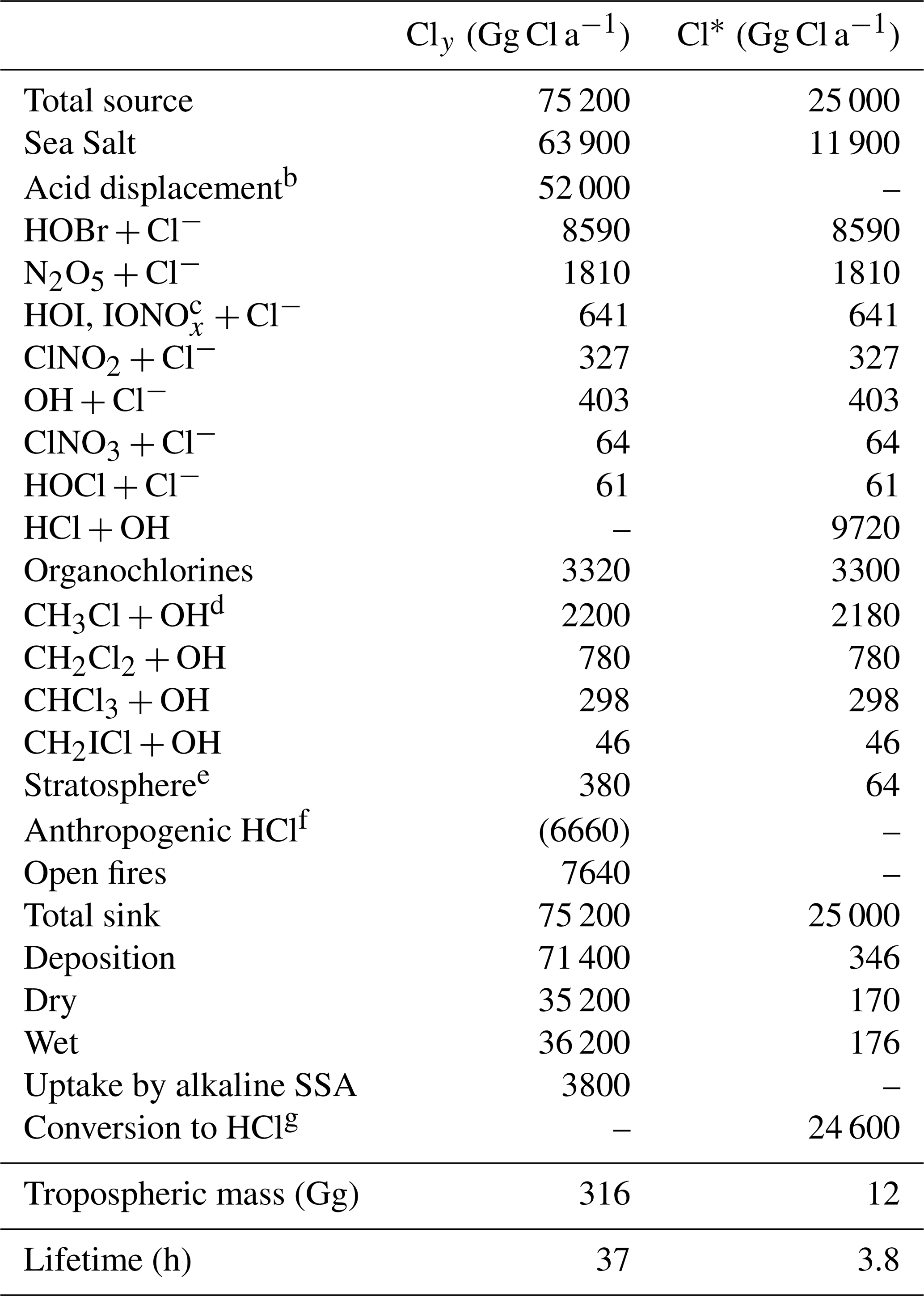
a Annual totals for 2016 computed from GEOS-Chem. Gas-phase inorganic chlorine is defined as . Reactive chlorine is defined as . Thus the source of HCl can be inferred from the Table entries as . The definition of Cly excludes aerosol Cl−, which has a very large sea salt source of 1780 Tg Cl a−1 but is mainly removed by deposition, HCl is the dominant component of Cly but is also mostly removed by deposition. Reactive chlorine Cl* is the chemical family principally involved in radical cycling. b Net production minus loss of HCl from acid aerosol displacement by HNO3 and H2SO4 computed as thermodynamic equilibrium. c . d The source from CH3Cl+Cl is not shown since it contributes <1 % of CH3Cl oxidation. Same for other organochlorines. e Net stratospheric input to the troposphere. f Coal combustion, waste incineration, and industrial activities. These emissions are only included in a sensitivity simulation (see Sects. 2.2 and 4.2 for details) and are therefore listed here in parentheses. Emissions of anthropogenic fugitive dust are estimated as less than 390 Gg a−1 (Sect. 2.2) and are not included in the model. g From reactions of Cl atoms (see Fig. 1).
Cl* can also be produced in the model by atmospheric degradation of the organochlorine gases CH3Cl, CH2Cl2, CHCl3, and CH2ICl. These gases are mainly of biogenic marine origin, with the exception of CH2Cl2, which has a large industrial solvent source (Simmonds et al., 2006). Mean tropospheric lifetimes are 520 days for CH3Cl, 280 days for CH2Cl2, 260 days for CHCl3, and 0.4 days for CH2ICl. Emissions of CH3Cl, CH2Cl2, and CHCl3 are implicitly treated in the model by specifying monthly mean surface air boundary conditions in five latitude bands (60–90, 30–60, and 0–30∘ N, 0–30, and 30–90∘ S) from AGAGE observations (Prinn et al., 2018). Emission of CH2ICl is from Ordóñez et al. (2012), as described by Sherwen et al. (2016a). Tropospheric oxidation of hydrochlorofluorocarbons (HCFCs) is neglected as a source of Cl* because it is small compared to the other organochlorines. The stratospheric source of Cly from chlorofluorocarbons (CFCs), HCFCs, and CCl4 is included in the model on the basis of the Eastham et al. (2014) GEOS-Chem stratospheric simulation as described in Sect. 2.1. Tropospheric organochlorines give a global Cl* source of 3.3 Tg Cl a−1 in Table 1, smaller than that from heterogeneous SSA Cl− reactions (11.9 Tg Cl a−1) or oxidation of HCl by OH (9.7 Tg Cl a−1). The stratosphere is a minor global source of tropospheric Cl* (0.06 Tg Cl a−1) although it could be important in the upper troposphere (Schmidt et al., 2016).
We also include primary HCl emissions from open fires. We apply the emission factors of () from Lobert et al. (1999) for different vegetation types to the GFED4 (Global Fire Emissions Database) biomass burned inventory (van der Werf et al., 2010; Giglio et al., 2013), resulting in a global source of 7.6 Tg Cl a−1 emitted as HCl.
Anthropogenic sources of HCl include coal combustion, waste incineration, and industrial activities. The only global emission inventory is that of McCulloch et al. (1999), which gives a total of 6.7 Tg Cl a−1. As shown in Sect. 4.2, we find that this greatly overestimates atmospheric observations of HCl over the US. National inventories of HCl from coal combustion available for China (236 Gg Cl a−1 in 2012; Liu et al., 2018) and the US (69 Gg Cl a−1 in 2014; US EPA, 2018) are respectively 6 and 7 times lower than estimates of McCulloch et al. (1999) for those countries. We therefore choose not to include anthropogenic HCl emissions in our standard simulation, as they are small in any case from a global budget perspective. We show in Sect. 4.2 that we can account for HCl observations in continental air largely on the basis of the SSA Cl−source. We also do not consider Cl* generation from snow/ice surfaces, which could be important in the Arctic spring MBL (Liao et al., 2014) but is highly uncertain and would only affect a small atmospheric domain.
We do not include the anthropogenic Cl− source from fugitive dust, although it might be important in contributing to chloride levels in continental surface air (Sarwar et al., 2012). The global source of anthropogenic fugitive dust is estimated to be less than 13 Tg a−1 (Philip et al., 2017), of which 0.3 % by mass is estimated to be chloride (Reff et al., 2009). This corresponds to a chloride source of less than 0.39 Tg Cl a−1, negligible on a global scale.
2.3 acid displacement thermodynamics
SSA Cl− can be displaced to HCl by strong acids (H2SO4, HNO3) once the SSA is sufficiently aged that its initial supply of alkalinity () has been exhausted. The acid displacement is described by
with equilibrium constants from Fountoukis and Nenes (2007). Reaction (R1) must be treated as an equilibrium because HNO3 and HCl have comparable effective Henry's law constants. H2SO4 has a much lower vapor pressure so that Reaction (R2) fully displaces HCl. Additional displacement of HCl by does not take place because is a much weaker acid than HCl (Jacob et al., 1985).
Alkalinity initially prevents any acid displacement in freshly emitted SSA. Alkalinity is emitted as 0.07 mol equivalents kg−1 of dry SSA (Gurciullo et al., 1999) and is transported in the model as two separate tracers for fine and coarse SSA. It is consumed over time by uptake of acids (SO2, H2SO4, HNO3, and HCl) as described by Alexander et al. (2005), and once fully consumed it is set to zero (titration). The SSA is then diagnosed as acidified, enabling acid displacement by Reactions (R1)–(R2). In our simulation, alkalinity is titrated everywhere shortly after emission except in some areas of the Southern Ocean, which is consistent with the model results of Alexander et al. (2005) and Kasibhatla et al. (2018).
Observations in the MBL indicate that fine SSA is usually internally mixed with sulfate–nitrate–ammonium (SNA) aerosols while coarse SSA is externally mixed (Fridlind and Jacobson, 2000; Dasgupta et al., 2007). Acid displacement for the acidified fine SSA is thus computed by adding to the SNA thermodynamics. The local thermodynamic gas–aerosol equilibrium for the resulting system is calculated with ISORROPIA II (Fountoukis and Nenes, 2007). The calculation is performed assuming an aqueous aerosol even if relative humidity is below the deliquescence point (metastable state). NVCs (non-volatile cations) describe the sum of cations emitted as SSA and is treated in ISORROPIA II using Na+ as proxy. Here NVCs are emitted as 16.4 mol kg−1 of dry SSA to balance the emission of SSA anions including Cl−, alkalinity, and sea salt sulfate. The NVC concentration is determined locally from the mass concentration of the inert SSA tracer.
Acid displacement for acidified coarse SSA is assumed to be driven by uptake of strong acids from the gas phase, mainly HNO3 (Kasibhatla et al., 2018). The ISORROPIA II calculation is conducted with two gas species (HNO3 and HCl) and four aerosol species (NVC, Cl−, , and ). Here the sulfate includes only the emitted sea salt component and that produced by heterogeneous SO2 oxidation in coarse SSA (Alexander et al., 2005). In the case of coarse aerosols, there may be significant mass transfer limitation to reaching gas–aerosol thermodynamic partitioning (Meng and Seinfeld, 1996). To account for this limitation, the concentrations are adjusted after the ISORROPIA II calculation following the dynamic method of Pilinis et al. (2000). This two-step thermodynamics approach has been used in previous studies (Koo et al., 2003; Kelly et al., 2010).
2.4 Heterogeneous chemistry of Cl−
Table 2 lists the heterogeneous reactions of Cl− other than acid displacement. The loss rate of a gas species X due to reaction with Cl− is calculated following Jacob (2000):
Here nX is the number density of species X (molecules of X per unit volume of air), A is the aerosol or cloud surface area concentration per unit volume of air, r is the effective particle radius, Dg is the gas-phase molecular diffusion coefficient of X, c is the average gas-phase thermal velocity of X, and γ is the reactive uptake coefficient, which is a function of the aqueous-phase molar Cl− concentration [Cl−] (moles of Cl− per liter of water). Values of γ in Table 2 are mostly from recommendations by the International Union of Pure and Applied Chemistry (IUPAC) (Ammann et al., 2013).
Table 2Heterogeneous reactions of Cl−and reactive uptake coefficients (γ)a.
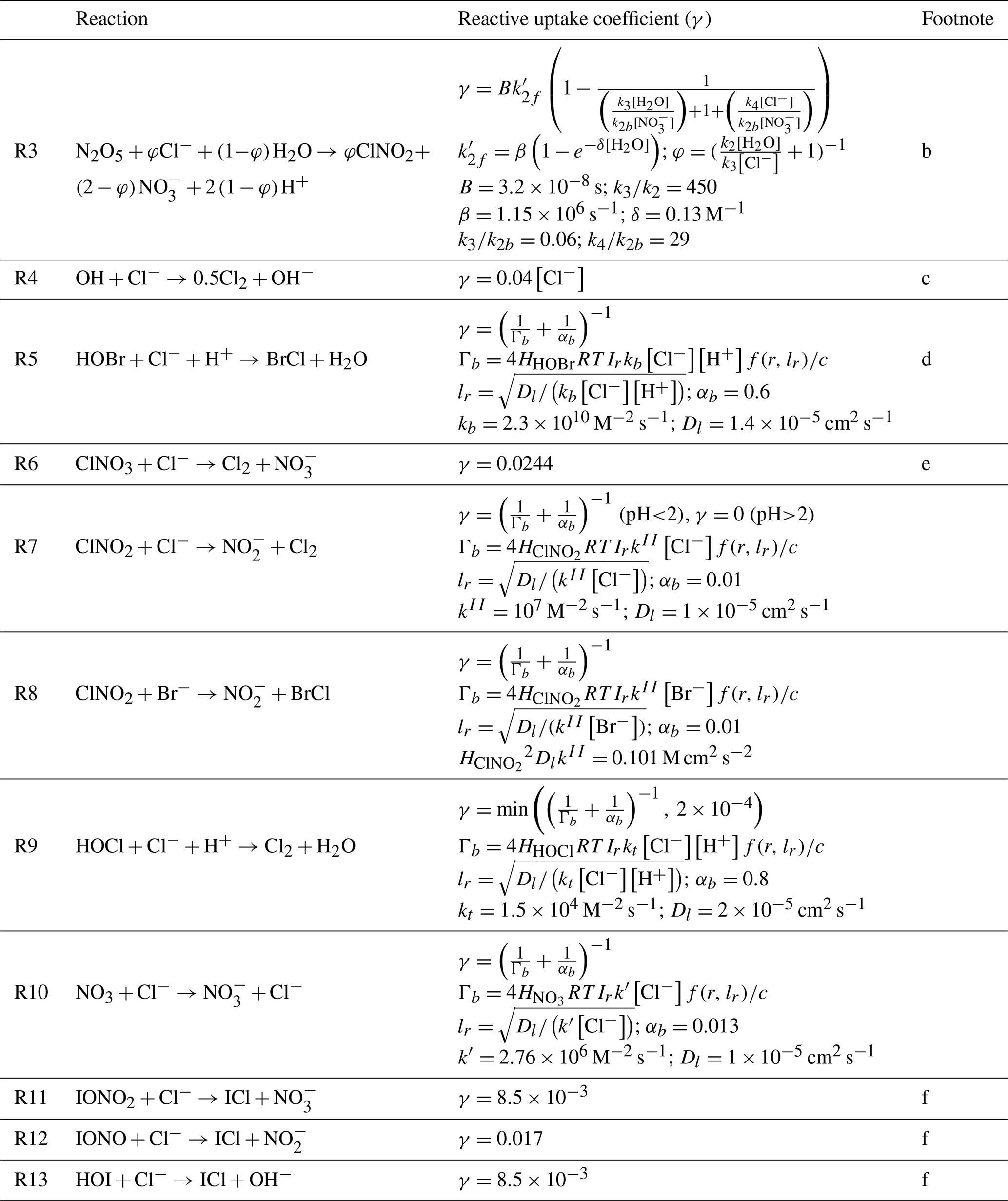
a Formulations for the reactive uptake coefficient γ are from IUPAC (Ammann et al., 2013) unless stated otherwise in the footnote column. Brackets denote aqueous-phase concentrations in molarity (moles per liter of water). R is the ideal gas constant. c is the average gas-phase thermal velocity for the reactant with Cl−. The reactive uptake coefficient is used to calculate the reaction rate following Eq. (1). is a spherical correction to mass transfer for which lr is a reacto-diffusive length scale and r is the radius of the aerosol particle or cloud droplet. b Bertram and Thornton (2009); Roberts et al. (2009). This parametrization is only applied for SNA and SSA aerosols. For N2O5 uptake on other aerosols, we assume φ=0 and follow Jaeglé et al. (2018). c Knipping and Dabdub (2002). d kb is based on Liu and Margerum (2001). Reaction (R5) competes with the heterogeneous reactions and HOBr+S(IV) as given by Chen et al. (2017). The BrCl product may either volatilize or react with Br− to produce Br2 and return Cl− following Fickert et al. (1999), as described in Sect. 5.2. e Assumes that Cl− is present in excess so that γ does not depend on [Cl−]. However, Reaction (R6) competes with the heterogeneous reaction as given by Schmidt et al. (2016), with the branching ratio determined by the relative rates. f These reactions are based on Sherwen et al. (2016a) and only take place in SSA.
The heterogeneous reactions take place in both clear-air aerosol and clouds. The GEOS-FP input meteorological data include cloud fraction and liquid/ice water content for every grid cell. Concentrations per cubic centimeter of air of aerosol-phase species (including fine and coarse Cl− and Br−) within a grid cell are partitioned between clear air and cloud as determined by the cloud fraction. Clear-air aqueous-phase concentrations for use in calculating heterogeneous reaction rates are derived from the relative-humidity-dependent liquid water contents of fine and coarse SSA using aerosol hygroscopic growth factors from the Global Aerosol Database (GADS, Koepke, 1997) with an update by Lewis and Schwartz (2006). In-cloud aqueous-phase concentrations are derived using liquid and ice water content from the GEOS-FP meteorological data. Values of r in Eq. (1) are specified as relative-humidity-dependent effective radii for the different clear-air aerosol components (Martin et al., 2003), and are set to 10 µm for cloud droplets and 75 µm for ice particles. These effective radii are also used to infer the area concentrations A on the basis of the mass concentrations. Heterogeneous chemistry in ice clouds is restricted to the unfrozen layer coating the ice crystal, which is assumed to be 1 % of the ice crystal radius (Schmidt et al., 2016).
The heterogeneous uptake of HOBr, HOCl, and ClNO2 as well as further aqueous-phase reaction with Cl− in Table 2 are pH dependent, with a higher efficiency in acidic solutions (Fickert et al., 1999; Roberts et al., 2008; Abbatt et al., 2012). They are considered only when SSA alkalinity has been titrated, and further requires pH <2, following laboratory results presented in Roberts et al. (2008). The pH of chloride-containing fine aerosol after alkalinity has been titrated is calculated by ISORROPIA II. Liquid cloud water pH is calculated in GEOS-Chem following Alexander et al. (2012), with update to include Cl− and NVC. Coarse-mode SSA and ice cloud pH are assumed to be 5 and 4.5, respectively (Schmidt et al., 2016).
Figure 1 describes the global budget and cycling of tropospheric inorganic chlorine in GEOS-Chem. The dominant source of Cly is acid displacement from SSA. The global rate of Cly generation from acid displacement is 52 Tg Cl a−1, close to the observationally based estimate of 50 Tg Cl a−1 by Graedel and Keene (1995) and lower than the model estimate of 90 Tg Cl a−1 from Hossaini et al. (2016), who treated displacement of Cl− by HNO3 as an irreversible rather than thermodynamic equilibrium process. HCl is the largest reservoir of Cly in the troposphere, with a global mean tropospheric mixing ratio of 60 ppt (ppt ≡ pmol mol−1).
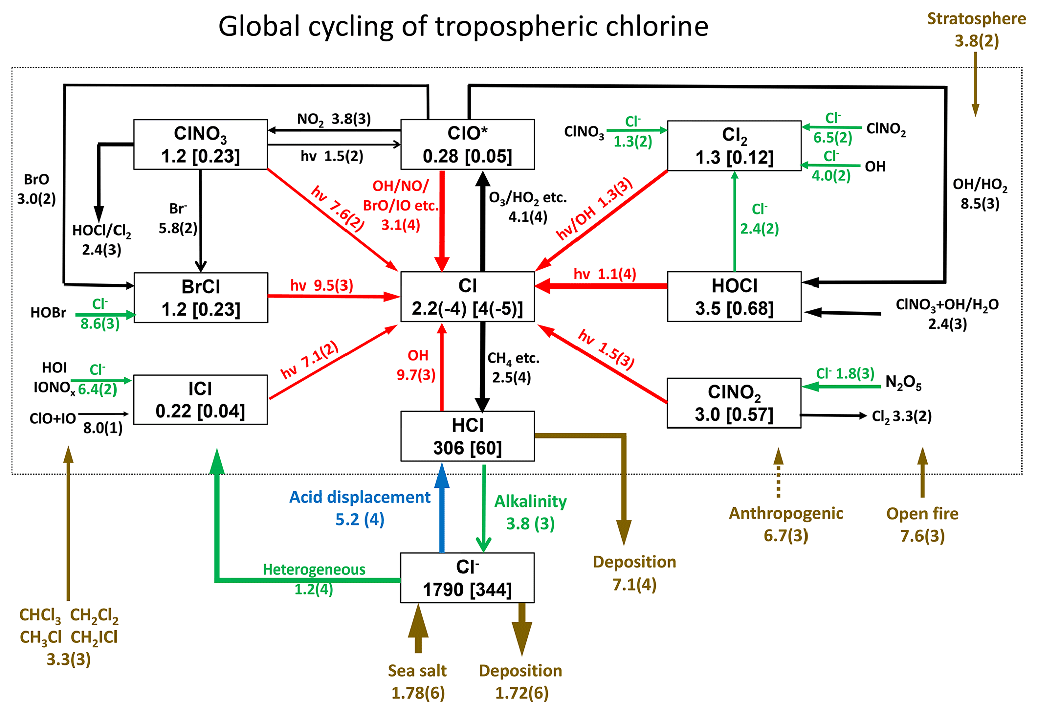
Figure 1Global budget and cycling of tropospheric inorganic chlorine (Cly) in GEOS-Chem. The figure shows global annual mean rates (Gg Cl a−1), masses (Gg), and mixing ratios (ppt, in brackets) for simulation year 2016. Read 2.5(4) as 2.5×10⁴. ClO* stands for ; 84 % is present as ClO. Reactions producing Cl atoms and related to Cl− heterogeneous chemistry are shown in red and green, respectively. The dotted box indicates the Cly family, and arrows into and out of that box represent general sources and sinks of Cly. Reactions with the rate <100 Gg Cl a−1 are not shown. Anthropogenic emissions of HCl as indicated by a dashed line are only included in a sensitivity simulation (see Sects. 2.2 and 4.2 for details).
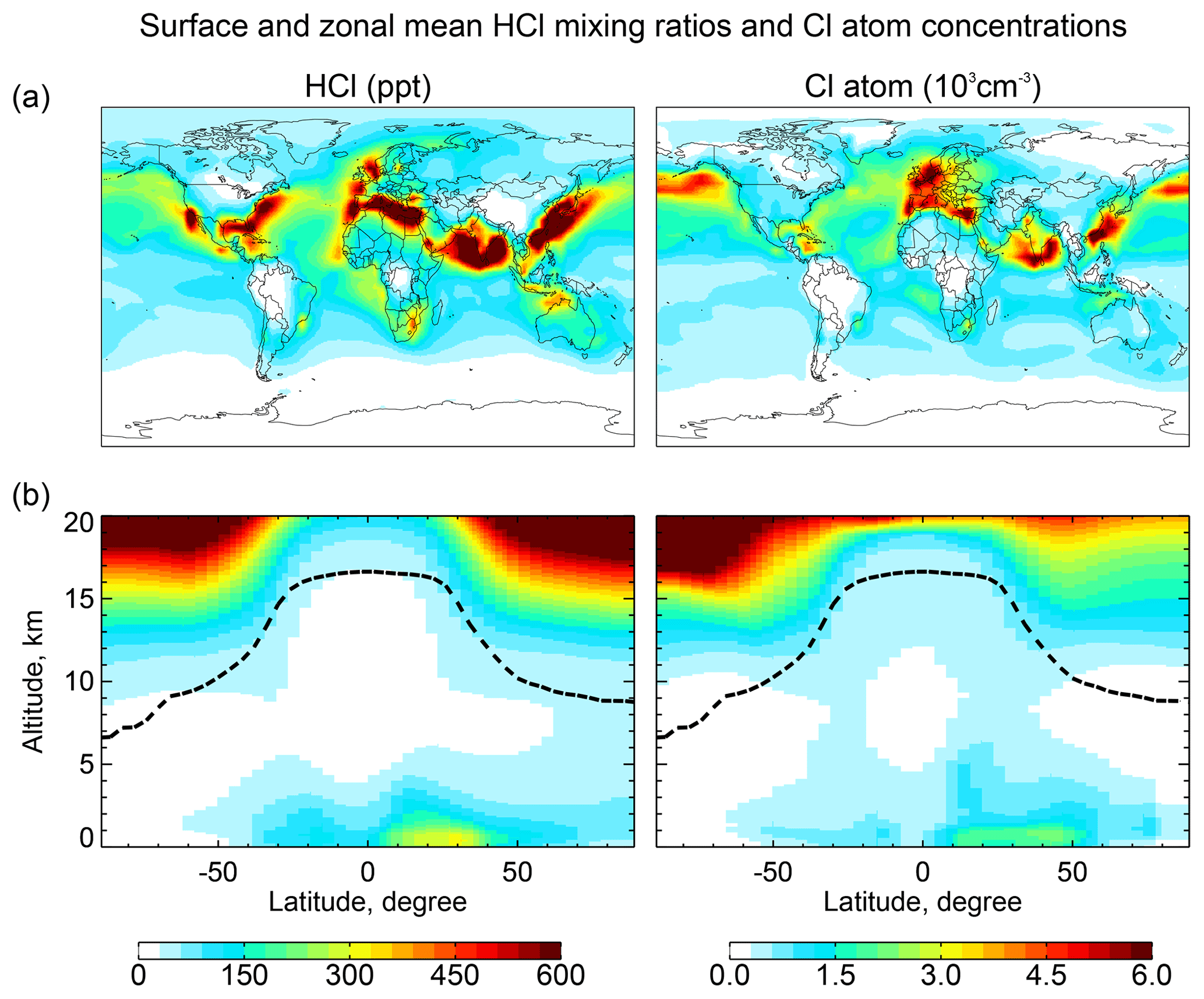
Figure 2Global distributions of annual mean HCl mixing ratios and Cl atom concentrations in GEOS-Chem. Panel (a) shows surface air mixing ratios and concentrations. Panel (b) shows zonal mean mixing ratios and concentrations as a function of latitude and altitude. Dashed lines indicate the tropopause.
Acid displacement generates Cly as HCl, which is mostly removed by deposition. Broader effects of chlorine on tropospheric chemistry take place through the cycling of radicals originating from production of reactive chlorine . HCl contributes 9.7 Tg Cl a−1 to Cl* through the reaction between HCl and OH. In addition to this source, Cl− provides a Cl* source of 12 Tg Cl a−1 through heterogeneous reactions with principal contributions from (8.6 Tg Cl a−1) and (1.8 Tg Cl a−1). This heterogeneous source of 12 Tg Cl a−1 is much higher than previous estimates of 5.6 Tg Cl a−1 (Hossaini et al., 2016) and 6.1 Tg Cl a−1 (Schmidt et al., 2016). Schmidt et al. (2016) only considered the reaction. Production of the chlorine radicals Cl and ClO is by the HCl+OH reaction (45 %) and by photolysis of BrCl (40 %), ClNO2 (8 %), Cl2 (4 %), and ICl (2 %). Loss of Cl* is mainly through the reaction of Cl with methane (46 %) and other organic compounds (CH3OH 15 %, CH3OOH 11 %, C2H6 8 %, higher alkanes 8 %, and CH2O 7 %).
Conversion of Cl to ClO* drives some cycling of chlorine radicals, but the associated chain length versus Cl* loss is short (). Conversion of Cl to ClO is mainly by reaction with ozone (98 %), while conversion of ClO back to Cl is mostly by reaction with NO (72 %), driving a null cycle as NO2 photolyzes to regenerate NO and ozone.
Figure 2 shows the annual mean global distributions of HCl mixing ratios and Cl atom concentrations. The mixing ratio of HCl decreases from the surface to the middle troposphere, reflecting the SSA source, and then increases again in the upper troposphere where it is supplied by transport from the stratosphere and has a long lifetime due to lack of scavenging. Remarkably, Cl atom concentrations show little decrease with altitude, contrary to the common assumption that tropospheric Cl atoms should be mainly confined to the MBL where the SSA source resides (Singh et al., 1996). We find that the effect of the SSA source is offset by the slower sink of Cl* at higher altitudes due to the strong temperature dependence of the reactions between Cl atom and organic compounds. Transport of HCl and Cl* from the stratosphere also contribute to the source of Cl atoms in the upper troposphere.
HCl mixing ratios in marine surface air are usually highest along polluted coastlines where the large sources of HNO3 and H2SO4 from anthropogenic NOx and SO2 emissions drive acid displacement from SSA. By contrast, HCl mixing ratios over the Southern Ocean are low because of the low supply of acid gases. The distribution of Cl atoms in surface air reflects its sources from both HCl+OH and the heterogeneous production of Cl*. The highest concentrations are in northern Europe due to production of ClNO2 from the Reaction (R3). Cl atom concentrations in marine air are shifted poleward relative to HCl because of increasing bromine radical concentrations (Parrella et al., 2012), driving BrCl formation by the Reaction (R5).
Figure 3 shows the global mean vertical distributions of reactive chlorine species (Cl*) in continental and marine air. Mean boundary layer mixing ratios are higher over land than over the ocean because of the ClNO2 source from in high-NOx polluted air (Thornton et al., 2010). ClNO2 mixing ratios are much higher than in the Sherwen et al. (2016b) model, which restricted its production to SSA, reflecting the importance of HCl dissolved in SNA aerosol, which allows further transport inland. High mixing ratios of ClNO3 in the upper troposphere are due to transport from the stratosphere and inefficacy of the sinks from hydrolysis and heterogeneous chemistry. In the marine MBL we find comparable contributions from HOCl (mainly in daytime) and Cl2 and ClNO2 (mainly at night). The BrCl mixing ratio is much lower than in the previous model studies of Long et al. (2014) and Sherwen et al. (2016b), which had very large sources from the Reaction (R5). Our lower BrCl mixing ratio is due to competition from the HOBr + S(IV) (S(IV) ) reaction (Chen et al., 2017) and to oceanic VOC emissions (Millet et al., 2010), both of which act to depress bromine radical concentrations in the MBL (Zhu et al., 2018). Further discussion of the BrCl source is presented in Sect. 5.2.
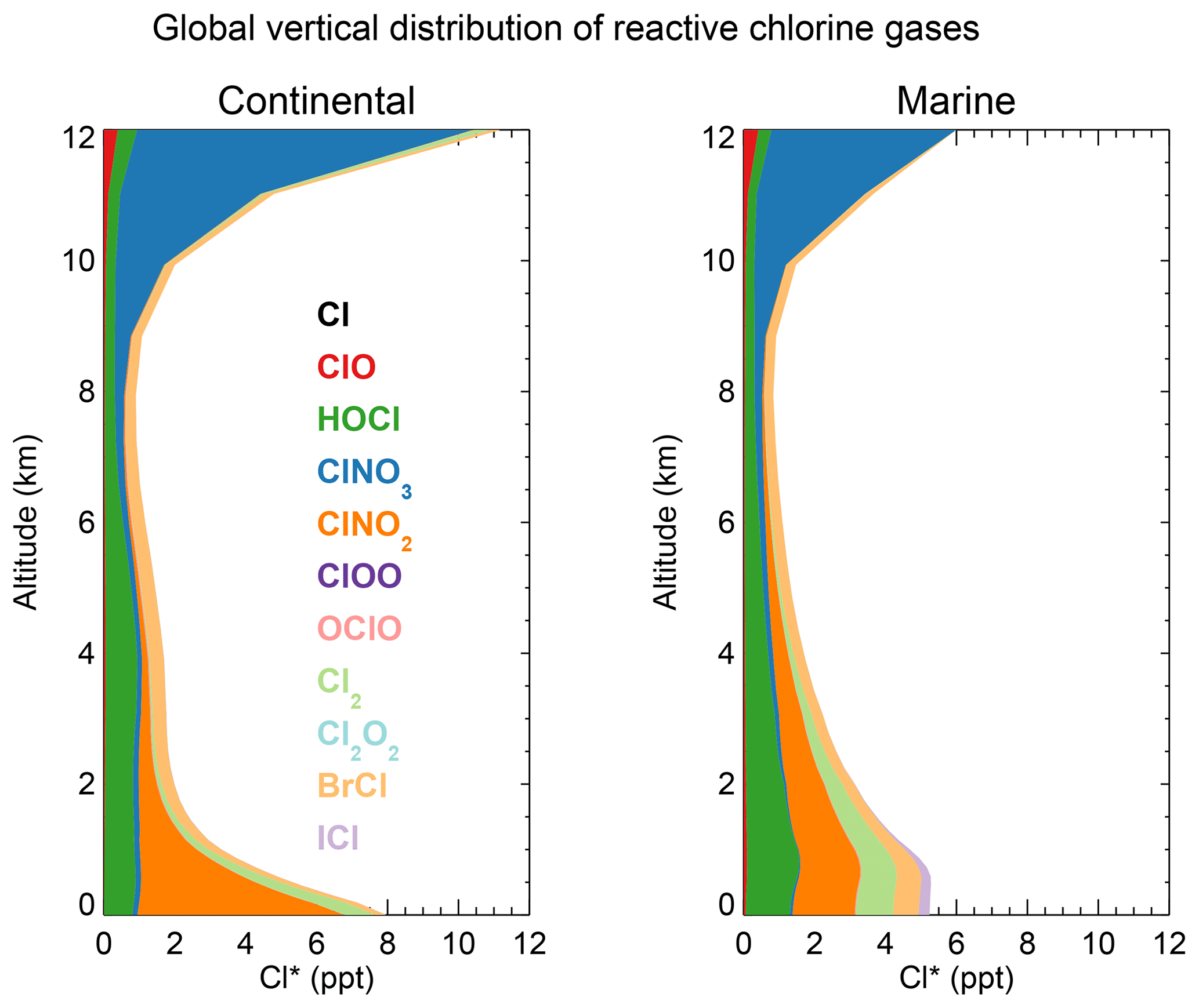
Figure 3Global annual mean vertical distributions of reactive chlorine species (Cl*) in GEOS-Chem for continental and marine air. Stratospheric conditions are excluded.
Here we compare the model simulation for 2016 to observations for gas-phase chlorine and related species collected in different years, assuming interannual variability to be a minor factor in model error. Previous evaluation of the GEOS-Chem sea salt source by Jaeglé et al. (2011) showed general skill in simulating SSA observations and we do not repeat this evaluation here. We also do not consider data affected by local anthropogenic sources because they would not be properly resolved at the grid resolution of our model.
4.1 Surface air observations
Table 3 compares our simulated Cl− SSA deficits to an ensemble of marine air observations compiled by Graedel and Keene (1995). The Cl− deficit is relative to seawater composition and provides an indicator of the mobilization of Cl− through acid displacement and heterogeneous chemistry. The observations show a wide range from −50 % to +90 %, and Graedel and Keene (1995) emphasize that uncertainties are large. Slight negative deficits in the observations could be caused by titration of alkalinity by HCl but large negative deficits are likely due to error. Mean model deficits sampled for the regions and months of the observations range from +4 to +40 %, not inconsistent with the observations. The largest model deficits are in polluted coastal regions because of acid displacement and this is also where the measured deficits are largest.
Table 3Chloride deficits in sea salt aerosola.
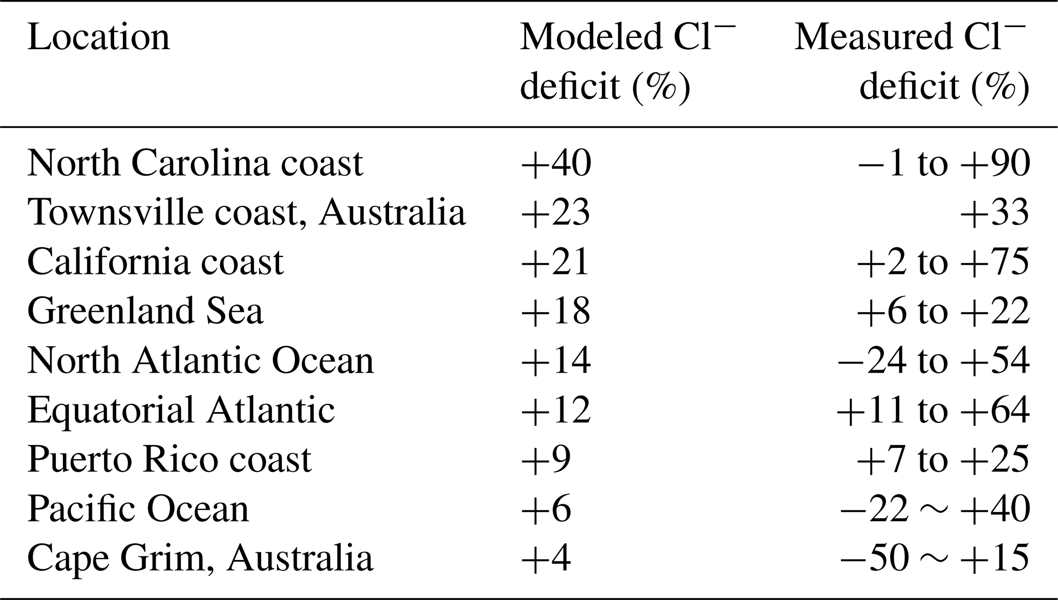
a Deficits relative to seawater composition. Observations compiled by Graedel and Keene (1995) are reported there as ranges for individual regions and months, with the ranges likely reflecting measurement uncertainty rather than physical variability. Model values are means for the regions and months of observations.
Figure 4 compares simulated HCl and HNO3 mixing ratios to concurrent observations of gases both at coastal sites and over oceans. The data are arranged from left to right by increasing latitude. Mean HCl mixing ratios average 323 ppt in the model and 347 ppt in the observations for the ensemble of regions. The HCl source in the model is mainly acid displacement from SSA. A sensitivity simulation without acid displacement from SSA has less than 7 ppt HCl in all regions. The model captures the spatial variability of the mean HCl mixing ratios across locations (r=0.88), which largely reflects the HCl enhancement at polluted coastal sites and northern midlatitudes (Fig. 2). Simulated HNO3 mixing ratios average 190 ppt across locations compared to 137 ppt in the observations, again with good simulation of spatial variability (r=0.96) driven by NOx emissions. HNO3 mixing ratios are sensitive to acid displacement from SSA, as the sensitivity simulation without acid displacement shows mean values of 441 ppt that are much higher than observed. This could partly explain the general model problem of HNO3 overestimation in remote air (Bey et al., 2001).
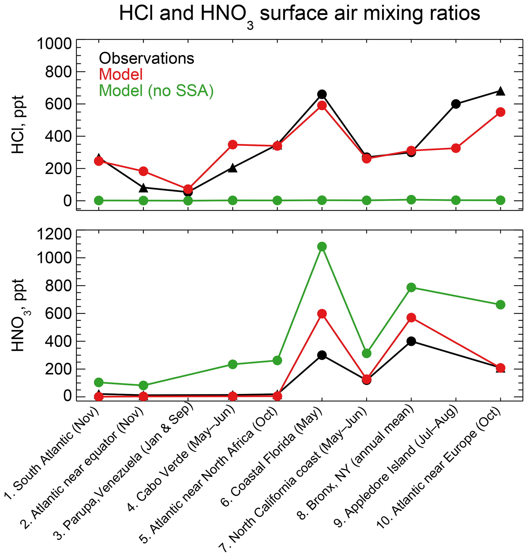
Figure 4HCl and HNO3 surface air mixing ratios at coastal and island sites and from ocean cruises, arranged from left to right in order of increasing latitude. Observations are means (black circles) or medians (black triangles) depending on availability from the publications. Model values are monthly means for the sampling locations. Also shown are results from a sensitivity simulation with no mobilization of Cl− from sea salt aerosol (SSA). References: (1, 2, 5, 10) Keene et al. (2009); (3) Sanhueza and Garaboto (2002); (4) Sander et al. (2013); (6) Dasgupta et al. (2007); (7) Crisp et al. (2014); (8) Bari et al. (2003); (9) Keene et al. (2007).
Figure 5 shows 2016 annual mean observations of PM2.5 Cl− (mass concentration in particles less than 2.5 µm diameter) from the US Interagency Monitoring of Protected Visual Environments (IMPROVE) network (Malm et al., 1994). Corresponding model values shown as background contours for fine Cl− (<1 µm diameter and internally mixed with SNA aerosol) are for total Cl−. One would expect the IMPROVE concentrations to be higher than the model fine Cl− (because of the larger size cut) and lower than total Cl−, and this is generally the case. The model is consistent with observations in the continental interior, which we attribute to inland transport of marine HCl incorporated into SNA aerosol. Fine Cl− concentrations can actually be higher over the continent than over the ocean because of HCl displacement from the coarse SSA followed by recondensation on anthropogenic SNA aerosol. The model underestimates the observations over the Southwest US and this may be due to a missing dust source. We find that IMPROVE Cl− and dust concentrations are positively correlated (R=0.3–0.9) in this region.
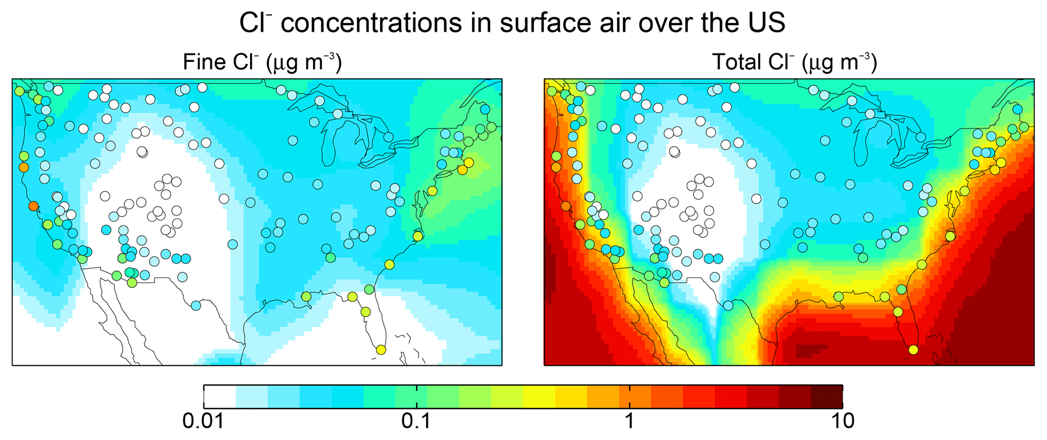
Figure 5Aerosol Cl− concentrations in surface air over the contiguous US. Values are annual means for 2016. GEOS-Chem model values are shown as contours separately for fine Cl− (<1 µm diameter) and total Cl−. Observations from the IMPROVE network (<2.5 µm diameter) are shown as circles and are the same in both panels; one would expect them to be higher than the model fine Cl− but lower than total Cl−.
Table 4Surface air mixing ratios of reactive chlorine (Cl*)a
a Reactive chlorine Cl* is the ensemble of gas-phase inorganic chlorine species excluding HCl. Measurements are 24 h averages. Model values are monthly means in 2016 taken for the same month and location as the observations. b Median value.
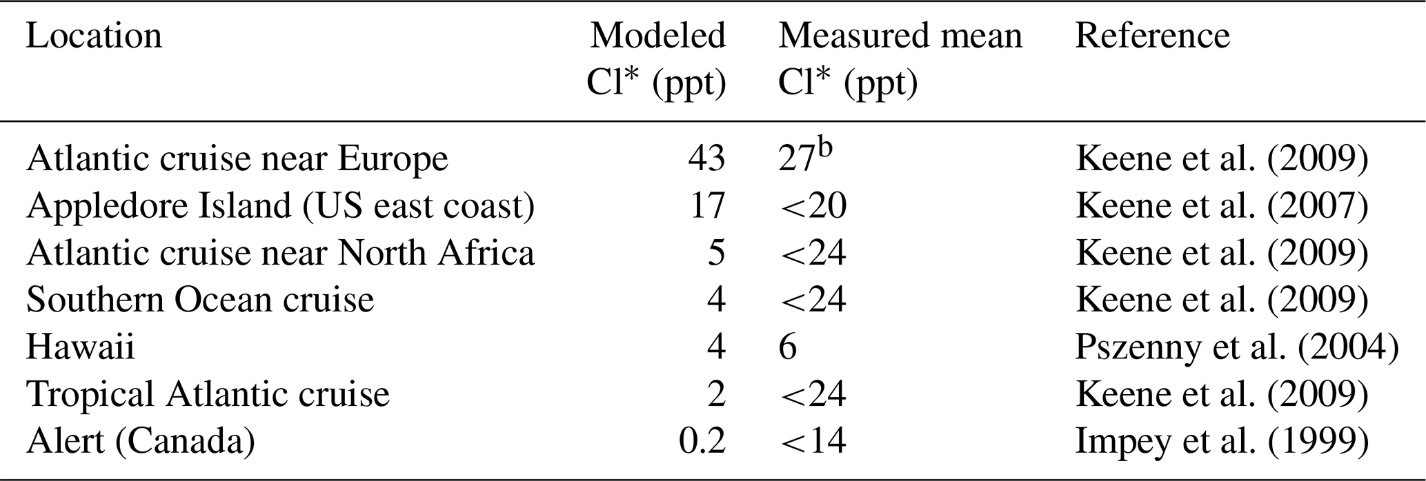
A number of surface air measurements have been made of Cl* as the water-soluble component of Cly after removal of HCl (Keene et al., 1990), although most of these measurements are below the detection limit (Table 4, mostly from Keene et al., 2009). This Cl* has been commonly assumed to represent the sum of Cl2 and HOCl (Pszenny et al., 1993) but it would also include ClNO2, ClNO3, and minor components of Cl*. Table 4 shows that simulated Cl* mixing ratios are consistent with the measurements to the extent that comparison is possible. Simulated Cl* over remote oceans is dominated by HOCl, but ClNO2 is responsible for the high values over the Atlantic Ocean near Europe.
Table 5Comparison of modeled maximum ClNO2 mixing ratios to surface observationsa.
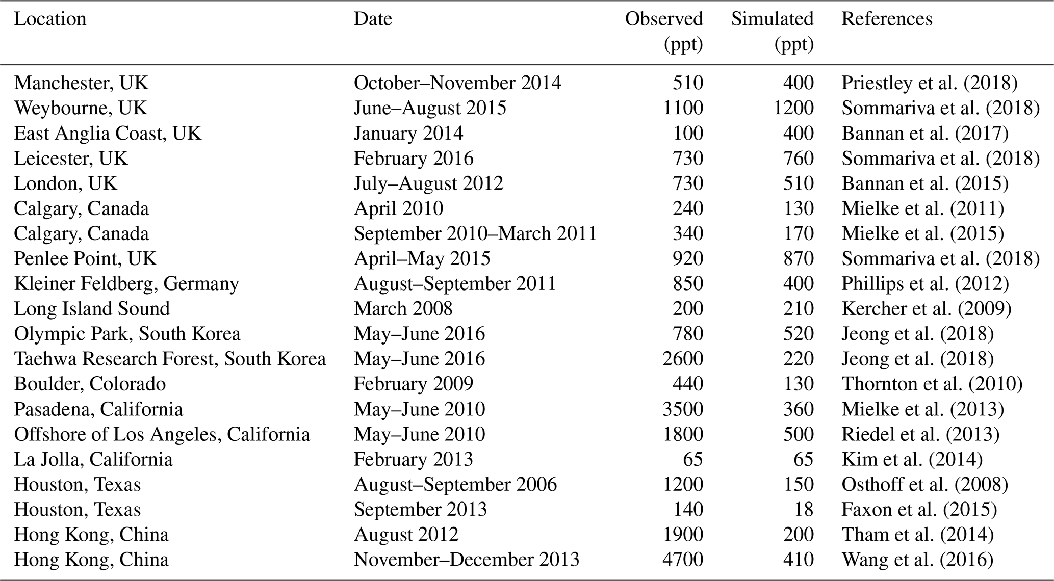
a Observed and modeled values are maxima for the reporting period. Model maxima are based on hourly values sampled at the same location and time period as the observations. The sites are listed in order of decreasing latitude.
Lawler et al. (2009) measured Cl2 and BrCl mixing ratios at Cabo Verde in the tropical Atlantic for 5 days in May–June 2007, and Lawler et al. (2011) measured Cl2 and HOCl mixing ratios at the same site for 7 days in May–June 2009. The observations show a diurnal cycle with mixing ratios of Cl2 highest at night, and HOCl highest in the day, consistent with the model. Observed mixing ratios in background marine air are in the range 0–30 ppt for Cl2 and 0–2 ppt for BrCl at night and 0–5 ppt for HOCl in the daytime. Corresponding mean model values are 0.3 ppt for Cl2, 1.8 ppt for BrCl, and 5 ppt for HOCl, with little day-to-day variability. Lawler et al. (2011) also sampled long-range outflow from Europe for 3 days in 2009 with daytime HOCl and nighttime Cl2 mixing ratio ranges of 40–200 and 5–40 ppt, respectively, but the model does not capture these enhancements. Sommariva and von Glasow (2012) suggested that a lower aerosol pH and/or slower rate for could explain the high HOCl in European outflow but this would also cause Cl2 to be lower. We have no explanation for the high Cl2 values observed by Lawler et al. (2009, 2011) in marine air or for the joint observed enhancements of HOCl and Cl2 in European outflow.
Many surface observations of ClNO2 have been made in nighttime urban environments. These are difficult to compare to the model because of the grid resolution and because of nighttime stratification of the surface layer (the lowest model grid level extends up to 130 m above the surface). In addition, the publications usually report maxima instead of means. Table 5 shows a comparison for representative sites, indicating that the model offers a credible simulation within the above caveats. The previous GEOS-Chem simulation of Sherwen et al. (2016b) only considered ClNO2 production in SSA and as a result their ClNO2 mixing ratios were consistently below a few parts per trillion at continental sites. Our simulation can reproduce the observed >100 ppt concentrations at these sites because it accounts for HCl dissolved in SNA aerosol, allowing marine influence to extend further inland as also shown in the comparison to the IMPROVE Cl− data (Fig. 5).
4.2 Comparison to aircraft measurements
The WINTER aircraft campaign over the eastern US and offshore in February–March 2015 provides a unique data set for evaluating our model. Measurements included HCl, ClNO2, HOCl, Cl2, and ClNO3 by iodide, time of flight, chemical ionization mass spectrometry (I-TOF-CIMS) (Lee et al., 2018). We focus on the first four measurements because calibration for ClNO3 needs further examination. The mean 1 s detection limits for HCl, ClNO2, HOCl, and Cl2 were 100, 2, 2, and 1 ppt, respectively (Lee et al., 2018). The estimated calibration uncertainty is ±30 % for all chlorine species. As discussed in Lee et al. (2018), labeled 15-N2O5 was added to the inlet tip during WINTER flights to quantify inlet production of ClNO2, which was found to be negligible (≪10 % of measured ClNO2), but inlet production of Cl2, for example from surface reactions of HOCl with adsorbed HCl, was not evaluated.
Figure 6 compares the observed median vertical profiles of HCl, ClNO2, HOCl, and Cl2 in WINTER to the model sampled along the flight tracks for the corresponding period. Figure 7 compares the median diurnal variations below 1 km in altitude, separately over ocean and land. We exclude daytime (10:00–16:00 local) data for ClNO2 in Fig. 6 because its mixing ratios are near zero (Fig. 7).

Figure 6Vertical profiles of HCl, nighttime ClNO2, HOCl, and Cl2 mixing ratios during the WINTER campaign over the eastern US and offshore in February–March 2015. Observations from Haskins et al. (2018) are shown as individual 1 min data points, with medians and 25th–75th percentiles in 500 m vertical bins. Measurements below the detection limit are treated as the median of 0 and detection limit. ClNO2 data exclude daytime (10:00–16:00 local) when mixing ratios are near zero in both the observations and the model (Fig. 7). Model values are shown as medians sampled along the flight tracks. Also shown are results from a sensitivity simulation including the anthropogenic chlorine inventory of McCulloch et al. (1999).
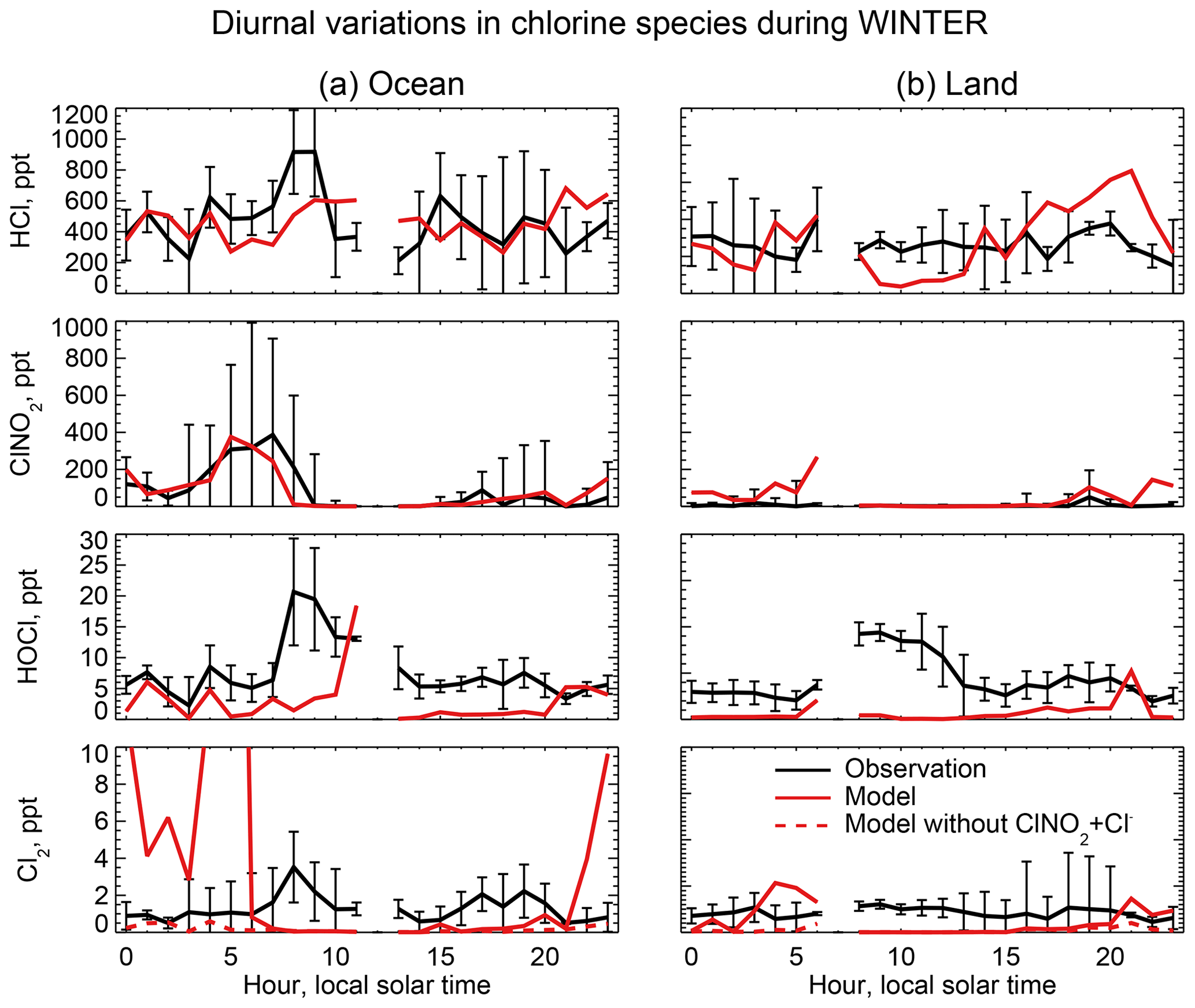
Figure 7Median diurnal variations in HCl, ClNO2, and Cl2 mixing ratios below 1 km in altitude during the WINTER aircraft campaign over the eastern US and offshore in February–March 2015. The data are separated between ocean (a) and land (b). Model values are compared to observations from Haskins et al. (2018). Vertical bars show the 25th–75th percentiles in the observations. Measurements below the detection limit are treated as the median of 0 and detection limit. Also shown are results from a sensitivity simulation excluding , which has a negligible effect on HCl, ClNO2, and HOCl but brings the Cl2 simulation in much better agreement with observations at night.
The WINTER observations of HCl show median values of 380 ppt near the surface, dropping to a background of 100–200 ppt in the free troposphere (Fig. 6). The model is lower than the observations in the lowest 2 km but within the calibration uncertainty. The free tropospheric background in the model is much lower than observed but the observations are near the 100 ppt detection limit. HCl mixing ratios in the lowest kilometer average 60 % higher over ocean than over land in both the observations and the model, reflecting the marine source.
Also shown in Fig. 6 is a sensitivity simulation including anthropogenic HCl emissions from McCulloch et al. (1999) as described in Sect. 2.2. The resulting model mixing ratios are too high though still within the calibration uncertainty. Based on sampling of power plant plumes during the WINTER campaign, Lee et al. (2018) inferred a HCl:SO2 emission mass ratio of 0.033 from power plants. Adding this emission to the standard simulation scaled to the SO2 emissions in GEOS-Chem (from the EPA National Emission Inventory over the US) increases modeled mixing ratios of HCl in the continental boundary layer by 18 % along the WINTER flight tracks, improving agreement with observations relative to the standard simulation but still representing a relatively minor source. ClNO2, HOCl, and Cl2 mixing ratios increase by 12 %, 8 %, and 4 %, respectively.
Figure 8 compares the model HCl vertical profiles to measurements by the Georgia Tech CIMS instrument during the SEAC4RS campaign over the Southeast US in August–September 2013 (Toon et al., 2016), the KORUS-AQ campaign over and around the Korean peninsula in May–June 2015, and the INTEX-B campaign over the North Pacific in May 2006 (Kim et al., 2008). The standard model simulation without anthropogenic chlorine successfully simulates the boundary layer HCl observations during SEAC4RS and KORUS-AQ but adding the McCulloch et al. (1999) anthropogenic inventory results in large overestimates. Boundary layer HCl mixing ratios over land are much lower in SEAC4RS than in WINTER and this is well reproduced by the model, for which the difference is due to seasonal contrast in the SSA source and in the inflow of marine air. The free tropospheric background observed in SEAC4RS, KORUS-AQ, and INTEX-B data is only ∼25 ppt, much lower than in WINTER (100–200 ppt), whereas the model free tropospheric background is consistently 20–50 ppt in all four campaigns. The WINTER observations are near their 100 ppt detection limit as pointed out above. The modeled vertical profile of HCl during INTEX-B is very similar to that of KORUS-AQ but overestimates observed boundary layer HCl by a factor of 5. The median value of observed surface HCl mixing ratio is 24 ppt during INTEX-B, which is much lower than all the surface air observations in Sect. 4.1.
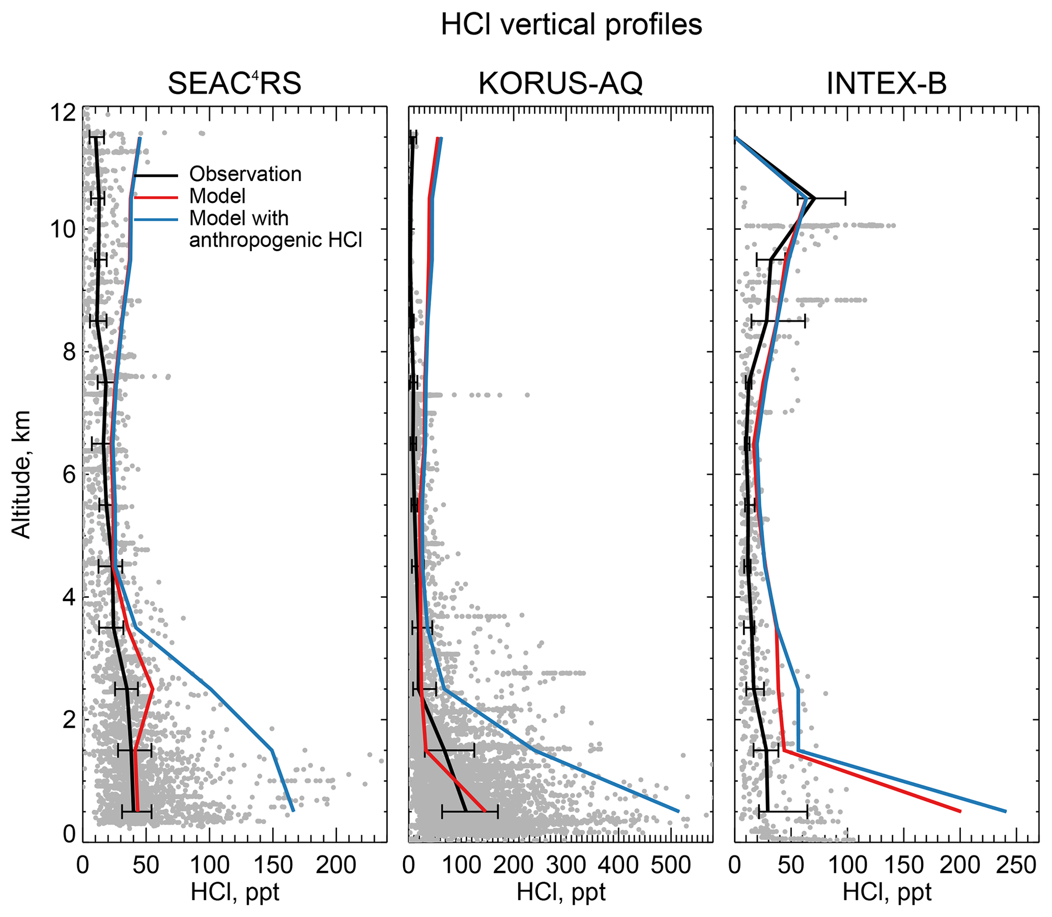
Figure 8Vertical profiles of HCl mixing ratios during the SEAC4RS aircraft campaign over the Southeast US (95–81.5∘ W, 30.5–39∘ N) in August–September 2013, during the KORUS-AQ aircraft campaign over and around the Korean peninsula (120–132∘ E, 32–38∘ N) in May–June 2015 and during the INTEX-B aircraft campaign over the North Pacific (175∘E–50∘ W, 40–61∘ N) in May 2006. Observations from the Georgia Tech CIMS instrument are shown as gray points (1 min averages), with medians and 25th–75th percentiles in 1 km vertical bins. Model values are sampled along the flight tracks and for the measurement period. Measurements below the detection limit are treated as the median of 0 and detection limit. Note the difference in scales among panels.
Mixing ratios of ClNO2 observed in WINTER are above the detection limit only in the lowest kilometer of atmosphere at night and are much higher over the ocean than over land. This is well simulated by the model (Figs. 6 and 7) and reflects the nighttime source from the heterogeneous reaction combined with the fast loss by photolysis in daytime. Previous studies have suggested that the Bertram and Thornton (2009) representation of the ClNO2 production yield from the heterogeneous reaction in Table 2 is too high (Riedel et al., 2013; Wagner et al., 2013; McDuffie et al., 2018a). By using a box model applied to the WINTER observations, McDuffie et al. (2018a, b) found that both the N2O5 uptake rate and the ClNO2 production yield were overestimated by the Bertram and Thornton (2009) parameterization. One important difference with these previous studies is the assumption of aerosol mixing state. GEOS-Chem assumes that Cl− is present only in SNA and SSA when doing the calculation of N2O5 reactive uptake rates, assuming an external mixture of aerosol types (Martin et al., 2003; Evans and Jacob, 2005; Jaeglé et al., 2018). This decreases both the N2O5 uptake rate and the ClNO2 yield compared to using the parameterization of Bertram and Thornton (2009) on internally mixed aerosols. Jaeglé et al. (2018) reported that using this external mixing assumption leads to good agreement between modeled and observed N2O5 during the WINTER campaign. The mean ClNO2 yield (φ in Reaction R3) below 1 km in our model is 0.20 during the WINTER campaign, very close to that calculated from observation (0.218) by McDuffie et al. (2018a).
Nighttime Cl2 mixing ratios in WINTER are greatly overestimated by the model. Under polluted wintertime conditions such as in WINTER the reaction greatly enhances Cl2 production in the model:
The reactive uptake coefficient for Reaction (R7) in Table 2 is based on a single laboratory study (Roberts et al., 2008). It requires an aerosol pH <2 and this condition is generally met for our model simulation of the WINTER environment, consistent with the observation-based analysis of aerosol pH by Guo et al. (2016) for the eastern US in winter. A sensitivity simulation without Reaction (R7) is shown as dashed red lines in Fig. 7 and can reproduce the low Cl2 mixing ratios observed over the ocean at night. The analysis of WINTER data by McDuffie et al. (2018b) finds that the correlation between particle acidity and Cl2 observations is opposite of the trend expected from Reaction (R7), though there may be no trend on sufficiently acidic (i.e., pH <2) aerosol. Further study of that reaction is needed. Similar reactions such as (Reaction R8) and are also very uncertain as their reaction rate coefficients are very different in different studies (Fickert et al., 1998; Frenzel et al., 1998; Schweitzer et al., 1998).
The model underestimates the WINTER observations of HOCl and Cl2 in daytime, over the ocean as well as over land. These species have short lifetimes due to photolysis (less than a few minutes). Direct anthropogenic emission from coal combustion has been proposed (Chang et al., 2002) but would only be observed in plumes and not over the oceans. Matching the >1 ppt Cl2 observed during daytime is particularly problematic since it would require a large photochemical source absent from the model. Lawler et al. (2011) suggested a fast daytime HOCl source from a hypothetical light-dependent Cl− oxidation. The measurements of Cl2 are also possibly subject to a positive artifact from rapid heterogeneous conversion of chlorine species on the surface of the TOF-CIMS inlet (Lee et al., 2018).
5.1 Cl atom and its impact on VOCs
The global mean pressure-weighted tropospheric Cl atom concentration in our simulation is 620 cm−3, while the MBL concentration averages 1200 cm−3 (Fig. 2). Our global mean is lower than the previous global model studies of Hossaini et al. (2016) (1300 cm−3) and Long et al. (2014) (3000 cm−3), which had excessive Cl* generation as discussed above. It is consistent with the upper limit of 1000 cm−3 inferred by Singh et al. (1996) from global modeling of C2Cl4 observations (C2Cl4 is highly reactive with Cl atoms). Isotopic observations of methane have been used to infer a Cl atom concentration in the MBL higher than 9000 cm−3 in the extratropical Southern Hemisphere (Platt et al., 2004; Allan et al., 2007), much higher than our estimate of 800 cm−3 over this region. More recently, Gromov et al. (2018) revisited these data together with added constraints from CO isotope measurements and concluded that extratropical Southern Hemisphere concentrations of Cl atoms in the MBL should be lower than 900 cm−3, consistent with our estimate.
Tropospheric oxidation by Cl atoms drives a present-day methane loss rate of 5.3 Tg a−1 in our model, contributing only 1.0 % of total methane chemical loss. It has a more significant impact on the oxidation of some other VOCs, contributing 20 % of the global loss for ethane, 14 % for propane, 10 % for higher alkanes, and 4 % for methanol.
5.2 Impact on bromine and iodine chemistry
Bromine radicals () and iodine radicals () affect global tropospheric chemistry by depleting ozone and OH (Parrella et al., 2012; Sherwen et al., 2016b). Br atoms are also thought to drive the oxidation of elemental mercury (Holmes et al., 2006). Chlorine chemistry increases IOx mixing ratios by 16 % due to the reactions of HOI, INO2, and INO3 with Cl− (Reactions R11–R13), producing ICl, which photolyzes rapidly to I atoms (Fig. 1). The effect on bromine is more complicated. Bromine radicals originate from photolysis and oxidation of organobromines emitted by the ocean, as well as from SSA de-bromination (Yang et al., 2005). They are lost by conversion to HBr, which is efficiently deposited. Parrella et al. (2012) pointed out that heterogeneous chemistry of HBr (dissolved as Br−) is critical for recycling bromine radicals and explaining observed tropospheric BrO mixing ratios in the background troposphere:
Chloride ions and dissolved SO2 can however compete with Br− for the available HOBr (Chen et al., 2017):
Chen et al. (2017) pointed out that Reaction (R16) effectively decreases BrO mixing ratios by producing HBr, which is rapidly deposited instead of contributing to BrOx cycling. They found in a GEOS-Chem simulation that global tropospheric BrO mixing ratios decreased by a factor of 2 as a result. Reaction (R5) may however have a compensating or opposite effect. It propagates the cycling of BrOx if BrCl volatilizes:
but it may also generate new BrOx if BrCl reacts with Br− in the aqueous phase to produce Br2 (Wang et al., 1994):
The sequence Reactions (R5) + (R18) + (R19) with Cl− as a catalyst has the same stoichiometry as Reaction (R14) and thus contributes to HBr recycling in the same way. We find in the model that it is globally 30 times faster than Reaction (R14) and therefore much more effective at regenerating bromine radicals. In GEOS-Chem, the rate of Reaction (R5) computed from Table 2 is applied to the following stoichiometry reflecting the ensemble of Reactions (R5), (R14), (R18), and (R19):
where Y is the yield of Br2 and 1−Y is the yield of BrCl. Y is calculated following the laboratory study of Fickert et al. (1999).
This mechanism was first included in GEOS-Chem version 11-02d by Chen et al. (2017), who did not however have an explicit SSA Cl− simulation (they instead assumed a fixed SSA [Cl−] =0.5 M, and considered only dissolved HCl in cloud).
Chen et al. (2017) found in their GEOS-Chem simulation that the global tropospheric BrO burden was 8.7 Gg without the HOBr+S(IV) Reaction (R16) and dropped to 3.6 Gg when that reaction was included. Previous GEOS-Chem model estimates of the global tropospheric BrO burden were 3.8 Gg (Parrella et al., 2012), 5.7 Gg (Schmidt et al., 2016), and 6.4 Gg (Sherwen et al., 2016b). Our simulation features many updates relative to Chen et al. (2017), including not only explicit SSA Cl− but also explicit calculation of aerosol pH with ISORROPIA II for the rates of reactions in Table 2. By including explicit SSA Cl−, the cloud water [Cl−] in our model is much higher than that in Chen et al. (2017) and more comparable to measurements ( M in typical cloud; Straub et al., 2007). We find in our standard simulation a global tropospheric BrO burden of 4.2 Gg, 17 % higher than that of Chen et al. (2017).
Figure 9 shows the change in surface BrO mixing ratios due specifically to tropospheric chlorine chemistry, as obtained by difference with a sensitivity simulation including none of the Cly chemistry shown in Fig. 1. The inclusion of chlorine chemistry increases the global tropospheric BrO burden by 85 %. More than 80 % of this change is caused by the reaction as discussed above. Other significant contributions include and . The largest BrO increases (1–2 ppt) are in surface air over the high-northern-latitude oceans where SSA emissions are high and acidic conditions promote chemistry.
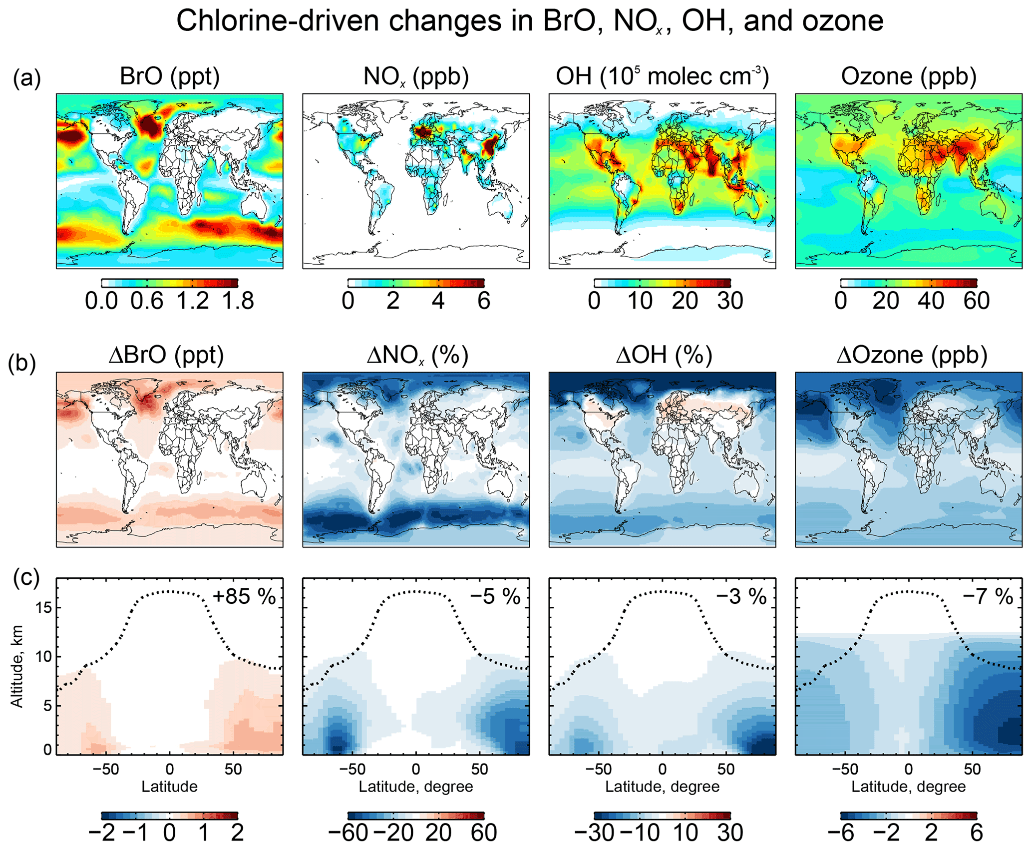
Figure 9Effects of tropospheric chlorine chemistry on BrO, NOx, OH, and ozone concentrations. Panel (a) shows the annual mean surface concentrations of BrO, NOx, OH, and ozone simulated in our standard model including tropospheric chlorine chemistry. Panels (b) and (c) show the changes in annual mean mixing ratios and concentrations due to tropospheric chlorine chemistry, as determined by the difference with a sensitivity simulation including no Cly production and cycling. Panel (b) shows the changes in surface air concentrations and panel (c) shows the changes in zonal mean mixing concentrations as a function of latitude and altitude. Black dashed lines indicate the tropopause. Numbers in (c) show the global tropospheric mean differences.
5.3 Impact on tropospheric ozone and OH
Figure 9 also shows the effects of chlorine chemistry on NOx, OH, and ozone concentrations. The global tropospheric burdens decrease by 5 % for NOx, 3 % for OH, and 7 % for ozone. The interhemispheric (N/S) ratio of tropospheric mean OH decreases from 1.14 to 1.12. Models tend to overestimate global mean tropospheric OH and its interhemispheric ratio relative to the constraint from methyl chloroform, which suggests a ratio of 0.85–0.98 (Naik et al., 2013; Voulgarakis et al., 2013). The effect of chlorine chemistry on the N∕S ratio is slight but in the right direction.
The chlorine-induced decreases in Fig. 9 are mainly through bromine chemistry initiated by chlorine (Sect. 5.2) and have spatial distributions characteristic of bromine chemistry with maxima at high latitudes as discussed by Schmidt et al. (2016). There are specific chlorine mechanisms including catalytic ozone loss through HOCl formation and photolysis:
and also loss of NOx:
However, we find that the rates are very small compared to similar mechanisms involving bromine and iodine because the stability of HCl quenches Cl* radical cycling.
A particular situation arises over polluted continents due to ClNO2 chemistry. Production of ClNO2 at night from the heterogeneous reaction, followed by photolysis in the morning to release Cl and NO2, provides a source of radicals and ozone. This explains the increases in OH over North America and Europe in Fig. 9. The effect is most important at high northern latitudes in winter due to the longer night. To isolate the impact on ozone we conducted a sensitivity simulation with no ClNO2 production, setting φ=0 for Reaction (R3) in Table 2. The surface air ozone enhancement due to ClNO2 chemistry is found to be the largest (∼8 ppb) in European winter, due to the large supply of Cl− from the North Atlantic combined with high NOx emissions. Other polluted continents see ozone increases of 1–5 ppb in winter. The effect in summer is less than 1 ppb. These results are similar to previous regional modeling studies by Sarwar et al. (2014) and Sherwen et al. (2017).
Figure S1 shows the differences of BrO, NOx, OH, and ozone concentrations between our model and the standard GEOS-Chem model version 11-02d including SSA de-bromination. Our explicit treatment of chlorine chemistry and thermodynamic representation of aerosol pH increases the global tropospheric BrO burden by 40 %. Most of this change is caused by faster reaction at high latitudes, resulting from higher Cl− concentration in our model, particularly in cloud. The decrease in BrO in the tropical MBL is caused by an increase in aerosol pH (pH was previously assumed to be 0 for computation of bromine chemistry), which slows down the acid-catalyzed recycling of bromine by Reactions (R5) and (R14). Our computed global tropospheric burdens decrease by 4 % for NOx, 2 % for OH, and 4 % for ozone relative to version 11-02d, again due to the more active bromine chemistry. The increase in OH over continental regions is due to our accounting of HCl dissolved in SNA aerosol, allowing marine influence to extend further inland to drive ClNO2 chemistry.
We have added to the GEOS-Chem model a comprehensive and consistent representation of tropospheric chlorine chemistry. This includes, in particular, explicit accounting of the mobilization of sea salt aerosol (SSA) chloride (Cl−), by acid displacement of HCl as well as by other heterogeneous processes. Cycling of inorganic gas-phase chlorine species (Cly) generated from SSA and other sources is simulated and coupled to the model aerosol–oxidant–bromine–iodine chemistry. With our work, GEOS-Chem now has a complete simulation of halogen () chemistry in both the troposphere and stratosphere.
Emission of chlorine in the model is mainly as sea salt aerosol (1780 Tg Cl a−1). Other sources (combustion, organochlorines, stratospheric input) are also included but are small in comparison. Most of the sea salt aerosol chloride is removed by deposition, but 3.6 % is mobilized to inorganic gas-phase chlorine (Cly) through acid displacement to HCl (52 Tg a−1) and through other heterogeneous chemistry producing more reactive chlorine species (12 Tg a−1). We define reactive chlorine (Cl*) as the ensemble of Cly species excluding HCl and including Cl, ClO, Cl2, BrCl, HOCl, ClNO2, and ClNO3 plus other minor species. Oxidation of HCl by OH provides a Cl* source of 9.7 Tg a−1, comparable to the heterogeneous source from (8.6 Tg a−1). (1.8 Tg a−1) is also important in polluted environments. Cycling among Cl* species drives radical chlorine (Cl∕ClO) chemistry but chain lengths are limited by fast conversion to HCl and subsequent deposition.
HCl mixing ratios in the model are highest over the oceans downwind of polluted continents due to effective acid displacement from sea salt aerosol by HNO3 and H2SO4. Mixing ratios are much lower over the Southern Ocean where the supply of acids is low. The dominant daytime Cl* species is generally HOCl while BrCl, Cl2, and ClNO2 dominate at night. ClNO3 dominates in the upper troposphere due to stratospheric input. Chlorine atom concentrations are highest over Europe in winter due to ClNO2 chemistry and are otherwise high over the northern midlatitude oceans where the supply of acidity promotes Cl formation through both HCl and acid-catalyzed heterogeneous processes.
Comparison of model results to observations in marine surface air shows that the model is usually able to reproduce the range and distributions of observed sea salt aerosol chloride deficits, HCl mixing ratios, and Cl* mixing ratios. In particular, concurrent observations of HCl and HNO3 in coastal/marine air worldwide show high correlation with the model including high HCl mixing ratios at northern midlatitudes combined with depressed HNO3. Consideration of acid displacement greatly improves model agreement with HNO3 observations in marine air. The model can also successfully simulate observations of high ClNO2 at night including in continental air. The chlorine in that case originates from sea salt aerosol transported far inland following uptake of volatilized HCl by sulfate–nitrate–ammonium (SNA) aerosol. The model cannot reproduce the very high HOCl and Cl2 concentrations observed by Lawler et al. (2009, 2011) at Cabo Verde in the tropical Atlantic.
Comparisons of model results to aircraft campaign observations from WINTER (eastern US and offshore, February–March 2015), SEAC4RS (Southeast US, August–September 2013), and KORUS-AQ (Korean peninsula, April–June 2016) show general consistency for HCl vertical profiles. Continental boundary layer HCl mixing ratios in these campaigns can be mostly accounted for by the marine source transported inland, though power plants could make a minor contribution. WINTER observations also include ClNO2, Cl2, and HOCl. The observed ClNO2 is mainly confined to the nighttime marine boundary layer and is consistent with the model. Observed Cl2 concentrations at night are much lower than the model, which has a large source under the WINTER conditions from the heterogeneous reaction. The rate coefficient for this reaction is from only one laboratory study.
The model simulates a global mean Cl atom concentration of 620 cm−3 in the troposphere and 1200 cm−3 in the marine boundary layer (MBL), lower than previous global model studies that had excessive generation of Cl* but consistent with independent proxy constraints. We find that oxidation by Cl atoms accounts for only 1.0 % of the global loss of atmospheric methane but has larger effects on the global losses of ethane (20 %), propane (14 %), and methanol (4 %). Chlorine chemistry increases global tropospheric BrO by 85 % and decreases ozone and OH by 7 % and 3 %, respectively, relative to a sensitivity simulation with no chlorine chemistry. The large effect on BrO is due to production of bromine radicals by the heterogeneous reaction, and the decreases in ozone and OH are mainly through the induced bromine chemistry. An exception is winter conditions over polluted regions, for which ClNO2 chemistry increases ozone mixing ratios by up to 8 ppb.
The model code is available from the corresponding author upon request and will be made available to the community through the standard GEOS-Chem (http://www.geos-chem.org) in the future. Data of the WINTER campaign are available to the general public at https://www.eol.ucar.edu/field_projects/winter. Data of NASA SEAC4RS, KORUS-AQ, and INTEX-B missions are available to the general public through the NASA data archive (https://www-air.larc.nasa.gov/cgi-bin/ArcView/seac4rs, https://www-air.larc.nasa.gov/cgi-bin/ArcView/korusaq, and https://www-air.larc.nasa.gov/cgi-bin/ArcView/intexb). IMPROVE data are available through the Federal Land Manager Environmental database (http://views.cira.colostate.edu/fed). All links mentioned here were last accessed on 1 March 2019.
The supplement related to this article is available online at: https://doi.org/10.5194/acp-19-3981-2019-supplement.
XW, DJJ, and HL designed the study. XW developed the chlorine model code and performed the simulations and analyses. XW, SDE, MPS, LZ, QC, BA, TS, and MJE contributed to the GEOS-Chem halogen model development. BHL, JDH, FDL, and JAT conducted and processed the measurements during the WINTER campaign. GLH conducted and processed the measurements during the SEAC4RS, KORUS-AQ, and INTEX-B campaigns. XW and DJJ prepared the paper with contributions from all co-authors.
The authors declare that they have no conflict of interest.
This work was supported by the Atmospheric Chemistry Program of the US National Science Foundation and by the Joint Laboratory for Air Quality and Climate (JLAQC) between Harvard and the Nanjing University for Information Science and Technology (NUIST). Qianjie Chen and Becky Alexander were supported by the National Science Foundation (AGS 1343077). We thank Prasad S. Kasibhatla for insightful discussion. WINTER data are provided by NCAR/EOL under sponsorship of the National Science Foundation (https://www.eol.ucar.edu/field_projects/winter, last access: 1 March 2019). SEAC4RS, KORUS-AQ, and INTEX-B data are provided by NASA LaRC Airborne Science Data for Atmospheric Composition (https://www-air.larc.nasa.gov, last access: 1 March 2019). IMPROVE is a collaborative association of state, tribal, and federal agencies and international partners. The U.S. Environmental Protection Agency is the primary funding source, with contracting and research support from the National Park Service. The Air Quality Group at the University of California, Davis is the central analytical laboratory, with ion analysis provided by the Research Triangle Institute and carbon analysis provided by the Desert Research Institute.
This paper was edited by Rolf Sander and reviewed by three anonymous referees.
Abbatt, J. P. D., Lee, A. K. Y., and Thornton, J. A.: Quantifying trace gas uptake to tropospheric aerosol: recent advances and remaining challenges, Chem. Soc. Rev., 41, 6555–6581, https://doi.org/10.1039/C2CS35052A, 2012.
Alexander, B., Park, R. J., Jacob, D. J., Li, Q. B., Yantosca, R. M., Savarino, J., Lee, C. C. W., and Thiemens, M. H.: Sulfate formation in sea-salt aerosols: Constraints from oxygen isotopes, J. Geophys. Res.-Atmos., 110, D10307, https://doi.org/10.1029/2004JD005659, 2005.
Alexander, B., Allman, D. J., Amos, H. M., Fairlie, T. D., Dachs, J., Hegg, D. A., and Sletten, R. S.: Isotopic constraints on the formation pathways of sulfate aerosol in the marine boundary layer of the subtropical northeast Atlantic Ocean, J. Geophys. Res.-Atmos., 117, D06304, https://doi.org/10.1029/2011JD016773, 2012.
Allan, W., Struthers, H., and Lowe C. D.: Methane carbon isotope effects caused by atomic chlorine in the marine boundary layer: Global model results compared with Southern Hemisphere measurements, J. Geophys. Res.-Atmos., 112, D04306, https://doi.org/10.1029/2006jd007369, 2007.
Ammann, M., Cox, R. A., Crowley, J. N., Jenkin, M. E., Mellouki, A., Rossi, M. J., Troe, J., and Wallington, T. J.: Evaluated kinetic and photochemical data for atmospheric chemistry: Volume VI – heterogeneous reactions with liquid substrates, Atmos. Chem. Phys., 13, 8045–8228, https://doi.org/10.5194/acp-13-8045-2013, 2013.
Amos, H. M., Jacob, D. J., Holmes, C. D., Fisher, J. A., Wang, Q., Yantosca, R. M., Corbitt, E. S., Galarneau, E., Rutter, A. P., Gustin, M. S., Steffen, A., Schauer, J. J., Graydon, J. A., Louis, V. L. St., Talbot, R. W., Edgerton, E. S., Zhang, Y., and Sunderland, E. M.: Gas-particle partitioning of atmospheric Hg(II) and its effect on global mercury deposition, Atmos. Chem. Phys., 12, 591–603, https://doi.org/10.5194/acp-12-591-2012, 2012.
Atkinson, R.: Gas-Phase Tropospheric Chemistry of Volatile Organic Compounds: 1. Alkanes and Alkenes, J. Phys. Chem. Ref. Data, 26, 215–290, 1997.
Bannan, T. J., Booth, A. M., Bacak, A., Muller, J. B. A., Leather, K. E., Le Breton, M., Jones, B., Young, D., Coe, H., Allan, J., Visser, S., Slowik, J. G., Furger, M., Prévôt, A. S. H., Lee, J., Dunmore, R. E., Hopkins, J. R., Hamilton, J. F., Lewis, A. C., Whalley, L. K., Sharp, T., Stone, D., Heard, D. E., Fleming, Z. L., Leigh, R., Shallcross, D. E., and Percival, C. J.: The first UK measurements of nitryl chloride using a chemical ionization mass spectrometer in central London in the summer of 2012, and an investigation of the role of Cl atom oxidation, J. Geophys. Res.-Atmos., 120, 5638–5657, https://doi.org/10.1002/2014JD022629, 2015.
Bannan, T. J., Bacak, A., Le Breton, M., Flynn, M., Ouyang, B., McLeod, M., Jones, R., Malkin, T. L., Whalley, L. K., Heard, D. E., Bandy, B., Khan, M. A. H., Shallcross, D. E., and Percival, C. J.: Ground and Airborne U.K. Measurements of Nitryl Chloride: An Investigation of the Role of Cl Atom Oxidation at Weybourne Atmospheric Observatory, J. Geophys. Res.-Atmos., 122, 11154–111165, https://doi.org/10.1002/2017JD026624, 2017.
Bari, A., Ferraro, V., Wilson, L. R., Luttinger, D., and Husain, L.: Measurements of gaseous HONO, HNO3, SO2, HCl, NH3, particulate sulfate and PM2.5 in New York, NY, Atmos. Environ., 37, 2825–2835, https://doi.org/10.1016/s1352-2310(03)00199-7, 2003.
Behnke, W., George, C., Scheer, V., and Zetzsch, C.: Production and decay of ClNO2 from the reaction of gaseous N2O5 with NaCl solution: Bulk and aerosol experiments, J. Geophys. Res.-Atmos., 102, 3795–3804, https://doi.org/10.1029/96JD03057, 1997.
Bertram, T. H. and Thornton, J. A.: Toward a general parameterization of N2O5 reactivity on aqueous particles: the competing effects of particle liquid water, nitrate and chloride, Atmos. Chem. Phys., 9, 8351–8363, https://doi.org/10.5194/acp-9-8351-2009, 2009.
Bey, I., Jacob, D. J., Yantosca, R. M., Logan, J. A., Field, B. D., Fiore, A. M., Li, Q., Liu, H. Y., Mickley, L. J., and Schultz, M. G.: Global modeling of tropospheric chemistry with assimilated meteorology: Model description and evaluation, J. Geophys. Res.-Atmos., 106, 23073–23095, https://doi.org/10.1029/2001JD000807, 2001.
Chang, S., McDonald-Buller, E., Kimura, Y., Yarwood, G., Neece, J., Russell, M., Tanaka, P., and Allen, D.: Sensitivity of urban ozone formation to chlorine emission estimates, Atmos. Environ., 36, 4991–5003, https://doi.org/10.1016/S1352-2310(02)00573-3, 2002.
Chen, Q., Schmidt, J. A., Shah, V., Jaeglé, L., Sherwen, T., and Alexander, B.: Sulfate production by reactive bromine: Implications for the global sulfur and reactive bromine budgets, Geophys. Res. Lett., 44, 7069–7078, https://doi.org/10.1002/2017GL073812, 2017.
Crisp, T. A., Lerner, B. M., Williams, E. J., Quinn, P. K., Bates, T. S., and Bertram, T. H.: Observations of gas phase hydrochloric acid in the polluted marine boundary layer, J. Geophys. Res.-Atmos., 119, 6897–6915, https://doi.org/10.1002/2013JD020992, 2014.
Dasgupta, P. K., Campbell, S. W., Al-Horr, R. S., Ullah, S. M. R., Li, J., Amalfitano, C., and Poor, N. D.: Conversion of sea salt aerosol to NaNO3 and the production of HCl: Analysis of temporal behavior of aerosol chloride/nitrate and gaseous HCl∕HNO3 concentrations with AIM, Atmos. Environ., 41, 4242–4257, https://doi.org/10.1016/j.atmosenv.2006.09.054, 2007.
Eastham, S. D., Weisenstein, D. K., and Barrett, S. R. H.: Development and evaluation of the unified tropospheric–stratospheric chemistry extension (UCX) for the global chemistry-transport model GEOS-Chem, Atmos. Environ., 89, 52–63, https://doi.org/10.1016/j.atmosenv.2014.02.001, 2014.
Evans, M. J. and Jacob, D. J.: Impact of new laboratory studies of N2O5 hydrolysis on global model budgets of tropospheric nitrogen oxides, ozone, and OH, Geophys. Res. Lett., 32, L09813, https://doi.org/10.1029/2005GL022469, 2005.
Faxon, C., Bean, J., and Ruiz, L.: Inland Concentrations of Cl2 and ClNO2 in Southeast Texas Suggest Chlorine Chemistry Significantly Contributes to Atmospheric Reactivity, Atmosphere, 6, 1487–1506, https://doi.org/10.3390/atmos6101487, 2015.
Fickert, S., Helleis, F., Adams, J. W., Moortgat, G. K., and Crowley, J. N.: Reactive uptake of ClNO2 on aqueous bromide solutions, J. Phys. Chem. A, 102, 10689–10696, https://doi.org/10.1021/jp983004n, 1998.
Fickert, S., Adams, J. W., and Crowley, J. N.: Activation of Br2 and BrCl via uptake of HOBr onto aqueous salt solutions, J. Geophys. Res.-Atmos., 104, 23719–23727, https://doi.org/10.1029/1999JD900359, 1999.
Finlayson-Pitts, B. J.: The Tropospheric Chemistry of Sea Salt: A Molecular-Level View of the Chemistry of NaCl and NaBr, Chem. Rev., 103, 4801–4822, https://doi.org/10.1021/cr020653t, 2003.
Fountoukis, C. and Nenes, A.: ISORROPIA II: a computationally efficient thermodynamic equilibrium model for aerosols, Atmos. Chem. Phys., 7, 4639–4659, https://doi.org/10.5194/acp-7-4639-2007, 2007.
Frenzel, A., Scheer, V., Sikorski, R., George, C., Behnke, W., and Zetzsch, C.: Heterogeneous Interconversion Reactions of BRNO2, ClNO2, Br2, and Cl2, J. Phys. Chem. A, 102, 1329–1337, https://doi.org/10.1021/jp973044b, 1998.
Fridlind, A. M. and Jacobson, M. Z.: A study of gas-aerosol equilibrium and aerosol pH in the remote marine boundary layer during the First Aerosol Characterization Experiment (ACE 1), J. Geophys. Res.-Atmos., 105, 17325–17340, https://doi.org/10.1029/2000JD900209, 2000.
Giglio, L., Randerson, J. T., and van der Werf, G. R.: Analysis of daily, monthly, and annual burned area using the fourth-generation global fire emissions database (GFED4), J. Geophys. Res.-Biogeo., 118, 317–328, https://doi.org/10.1002/jgrg.20042, 2013.
Graedel, T. E. and Keene, W. C.: Tropospheric budget of reactive chlorine, Global Biogeochem. Cy., 9, 47–77, https://doi.org/10.1029/94GB03103, 1995.
Gromov, S., Brenninkmeijer, C. A. M., and Jöckel, P.: A very limited role of tropospheric chlorine as a sink of the greenhouse gas methane, Atmos. Chem. Phys., 18, 9831–9843, https://doi.org/10.5194/acp-18-9831-2018, 2018.
Guo, H., Sullivan, A. P., Campuzano-Jost, P., Schroder, J. C., Lopez-Hilfiker, F. D., Dibb, J. E., Jimenez, J. L., Thornton, J. A., Brown, S. S., Nenes, A., and Weber, R. J.: Fine particle pH and the partitioning of nitric acid during winter in the northeastern United States, J. Geophys. Res.-Atmos., 121, 10355–10376, https://doi.org/10.1002/2016JD025311, 2016.
Gurciullo, C., Lerner, B., Sievering, H., and Pandis, S. N.: Heterogeneous sulfate production in the remote marine environment: Cloud processing and sea-salt particle contributions, J. Geophys. Res., 104, 21719–21731, 1999.
Haskins, J. D., Jaeglé, L., Shah, V., Lee, B. H., Lopez-Hilfiker, F. D., Campuzano-Jost, P., Schroder, J. C., Day, D. A., Guo, H., Sullivan, A. P., Weber, R., Dibb, J., Campos, T., Jimenez, J. L., Brown, S. S., and Thornton, J. A.: Wintertime Gas-Particle Partitioning and Speciation of Inorganic Chlorine in the Lower Troposphere Over the Northeast United States and Coastal Ocean, J. Geophys. Res.-Atmos., 123, 12897–12916, https://doi.org/10.1029/2018JD028786, 2018.
Hoffmann, E. H., Tilgner, A., Schrödner, R., Bräuer, P., Wolke, R., and Herrmann, H.: An advanced modeling study on the impacts and atmospheric implications of multiphase dimethyl sulfide chemistry, P. Natl. Acad. Sci. USA, 113, 11776–11781, https://doi.org/10.1073/pnas.1606320113, 2016.
Holmes, C. D., Jacob, D. J., and Yang, X.: Global lifetime of elemental mercury against oxidation by atomic bromine in the free troposphere, Geophys. Res. Lett., 33, L20808, https://doi.org/10.1029/2006GL027176, 2006.
Horowitz, H. M., Jacob, D. J., Zhang, Y., Dibble, T. S., Slemr, F., Amos, H. M., Schmidt, J. A., Corbitt, E. S., Marais, E. A., and Sunderland, E. M.: A new mechanism for atmospheric mercury redox chemistry: implications for the global mercury budget, Atmos. Chem. Phys., 17, 6353–6371, https://doi.org/10.5194/acp-17-6353-2017, 2017.
Hossaini, R., Chipperfield, M. P., Saiz-Lopez, A., Fernandez, R., Monks, S., Feng, W., Brauer, P., and von Glasow, R.: A global model of tropospheric chlorine chemistry: Organic versus inorganic sources and impact on methane oxidation, J. Geophys. Res.-Atmos., 121, 14271–14297, https://doi.org/10.1002/2016JD025756, 2016.
Impey, G. A., Mihele, C. M., Anlauf, K. G., Barrie, L. A., Hastie, D. R., and Shepson, P. B.: Measurements of Photolyzable Halogen Compounds and Bromine Radicals During the Polar Sunrise Experiment 1997, J. Atmos. Chem., 34, 21–37, https://doi.org/10.1023/a:1006264912394, 1999.
Jacob, D. J.: Heterogeneous chemistry and tropospheric ozone, Atmos. Environ., 34, 2131–2159, https://doi.org/10.1016/S1352-2310(99)00462-8, 2000.
Jacob, D. J., Waldman, J. M., Munger, J. W., and Hoffmann, M. R.: Chemical composition of fogwater collected along the California coast, Environ. Sci. Technol., 19, 730–736, https://doi.org/10.1021/es00138a013, 1985.
Jaeglé, L., Quinn, P. K., Bates, T. S., Alexander, B., and Lin, J.-T.: Global distribution of sea salt aerosols: new constraints from in situ and remote sensing observations, Atmos. Chem. Phys., 11, 3137–3157, https://doi.org/10.5194/acp-11-3137-2011, 2011.
Jaeglé, L., Shah, V., Thornton, J. A., Lopez-Hilfiker, F. D., Lee, B. H., McDuffie, E. E., Fibiger, D., Brown, S. S., Veres, P., Sparks, T. L., Ebben, C. J., Wooldridge, P. J., Kenagy, H. S., Cohen, R. C., Weinheimer, A. J., Campos, T. L., Montzka, D. D., Digangi, J. P., Wolfe, G. M., Hanisco, T., Schroder, J. C., Campuzano-Jost, P., Day, D. A., Jimenez, J. L., Sullivan, A. P., Guo, H., and Weber, R. J.: Nitrogen Oxides Emissions, Chemistry, Deposition, and Export Over the Northeast United States During the WINTER Aircraft Campaign, J. Geophys. Res.-Atmos., 123, 12368–12393, https://doi.org/10.1029/2018JD029133, 2018.
Jeong, D., Seco, R., Gu, D., Lee, Y., Nault, B. A., Knote, C. J., Mcgee, T., Sullivan, J. T., Jimenez, J. L., Campuzano-Jost, P., Blake, D. R., Sanchez, D., Guenther, A. B., Tanner, D., Huey, L. G., Long, R., Anderson, B. E., Hall, S. R., Ullmann, K., Shin, H.-J., Herndon, S. C., Lee, Y., Kim, D., Ahn, J., and Kim, S.: Integration of Airborne and Ground Observations of Nitryl Chloride in the Seoul Metropolitan Area and the Implications on Regional Oxidation Capacity During KORUS-AQ 2016, Atmos. Chem. Phys. Discuss., https://doi.org/10.5194/acp-2018-1216, in review, 2018.
Kasibhatla, P., Sherwen, T., Evans, M. J., Carpenter, L. J., Reed, C., Alexander, B., Chen, Q., Sulprizio, M. P., Lee, J. D., Read, K. A., Bloss, W., Crilley, L. R., Keene, W. C., Pszenny, A. A. P., and Hodzic, A.: Global impact of nitrate photolysis in sea-salt aerosol on NOx, OH, and O?3 in the marine boundary layer, Atmos. Chem. Phys., 18, 11185–11203, https://doi.org/10.5194/acp-18-11185-2018, 2018.
Keene, W. C., Pszenny, A. A. P., Jacob, D. J., Duce, R. A., Galloway, J. N., Schultz-Tokos, J. J., Sievering, H., and Boatman, J. F.: The geochemical cycling of reactive chlorine through the marine troposphere, Global Biogeochem. Cy., 4, 407–430, https://doi.org/10.1029/GB004i004p00407, 1990.
Keene, W. C., Stutz, J., Pszenny, A. A. P., Maben, J. R., Fischer, E. V., Smith, A. M., von Glasow, R., Pechtl, S., Sive, B. C., and Varner, R. K.: Inorganic chlorine and bromine in coastal New England air during summer, J. Geophys. Res.-Atmos., 112, D10S12, https://doi.org/10.1029/2006jd007689, 2007.
Keene, W. C., Long, M. S., Pszenny, A. A. P., Sander, R., Maben, J. R., Wall, A. J., O'Halloran, T. L., Kerkweg, A., Fischer, E. V., and Schrems, O.: Latitudinal variation in the multiphase chemical processing of inorganic halogens and related species over the eastern North and South Atlantic Oceans, Atmos. Chem. Phys., 9, 7361–7385, https://doi.org/10.5194/acp-9-7361-2009, 2009.
Kelly, J. T., Bhave, P. V., Nolte, C. G., Shankar, U., and Foley, K. M.: Simulating emission and chemical evolution of coarse sea-salt particles in the Community Multiscale Air Quality (CMAQ) model, Geosci. Model Dev., 3, 257–273, https://doi.org/10.5194/gmd-3-257-2010, 2010.
Kercher, J. P., Riedel, T. P., and Thornton, J. A.: Chlorine activation by N2O5: simultaneous, in situ detection of ClNO2 and N2O5 by chemical ionization mass spectrometry, Atmos. Meas. Tech., 2, 193–204, https://doi.org/10.5194/amt-2-193-2009, 2009.
Kim, S., Huey, L. G., Stickel, R. E., Pierce, R. B., Chen, G., Avery, M. A., Dibb, J. E., Diskin, G. S., Sachse, G. W., McNaughton, C. S., Clarke, A. D., Anderson, B. E., and Blake, D. R.: Airborne measurements of HCl from the marine boundary layer to the lower stratosphere over the North Pacific Ocean during INTEX-B, Atmos. Chem. Phys. Discuss., 8, 3563–3595, https://doi.org/10.5194/acpd-8-3563-2008, 2008.
Kim, M. J., Farmer, D. K., and Bertram, T. H.: A controlling role for the air-sea interface in the chemical processing of reactive nitrogen in the coastal marine boundary layer, P. Natl. Acad. Sci. USA, 111, 3943–3948, https://doi.org/10.1073/pnas.1318694111, 2014.
Knipping, E. M. and Dabdub, D.: Modeling Cl2 formation from aqueous NaCl particles: Evidence for interfacial reactions and importance of Cl2 decomposition in alkaline solution, J. Geophys. Res.-Atmos., 107, 4360, https://doi.org/10.1029/2001JD000867, 2002.
Koepke, P., Hess, M., Schult, I., and Shettle, E. P.: Global Aerosol Data Set, Report No. 243, Max-Planck-Institut für Meteorologie, Hamburg, 1997.
Kolesar, K. R., Mattson, C. N., Peterson, P. K., May, N. W., Prendergast, R. K., and Pratt, K. A.: Increases in wintertime PM2.5 sodium and chloride linked to snowfall and road salt application, Atmos. Environ., 177, 195–202, https://doi.org/10.1016/j.atmosenv.2018.01.008, 2018.
Koo, B., Gaydos, T. M., and Pandis, S. N.: Evaluation of the Equilibrium, Dynamic, and Hybrid Aerosol Modeling Approaches, Aerosol. Sci. Tech., 37, 53–64, https://doi.org/10.1080/02786820300893, 2003.
Lawler, M. J., Finley, B. D., Keene, W. C., Pszenny, A. A. P., Read, K. A., von Glasow, R., and Saltzman, E. S.: Pollution-enhanced reactive chlorine chemistry in the eastern tropical Atlantic boundary layer, Geophys. Res. Lett., 36, L08810, https://doi.org/10.1029/2008gl036666, 2009.
Lawler, M. J., Sander, R., Carpenter, L. J., Lee, J. D., von Glasow, R., Sommariva, R., and Saltzman, E. S.: HOCl and Cl2 observations in marine air, Atmos. Chem. Phys., 11, 7617–7628, https://doi.org/10.5194/acp-11-7617-2011, 2011.
Lee, B. H., Lopez-Hilfiker, F. D., Schroder, J. C., Campuzano-Jost, P., Jimenez, J. L., McDuffie, E. E., Fibiger, D. L., Veres, P. R., Brown, S. S., Campos, T. L., Weinheimer, A. J., Flocke, F. F., Norris, G., O'Mara, K., Green, J. R., Fiddler, M. N., Bililign, S., Shah, V., Jaeglé, L., and Thornton, J. A.: Airborne Observations of Reactive Inorganic Chlorine and Bromine Species in the Exhaust of Coal-Fired Power Plants, J. Geophys. Res.-Atmos., 123, 11225–11237, https://doi.org/10.1029/2018jd029284, 2018.
Lewis, E. and Schwartz, S.: Comment on “size distribution of sea-salt emissions as a function of relative humidity”, Atmos. Env., 40, 588–590, 2006.
Lewis, E. and Schwartz, S.: Sea Salt Aerosol Production: Mechanisms, Methods, Measurements and Models, Geophys. Monogr. Ser., Vol. 152, AGU, Washington, D.C., https://doi.org/10.1029/GM152, 2014.
Liao, J., Huey, L. G., Liu, Z., Tanner, D. J., Cantrell, C. A., Orlando, J. J., Flocke, F. M., Shepson, P. B., Weinheimer, A. J., Hall, S. R., Ullmann, K., Beine, H. J., Wang, Y., Ingall, E. D., Stephens, C. R., Hornbrook, R. S., Apel, E. C., Riemer, D., Fried, A., Mauldin, R. L., Smith, J. N., Staebler, R. M., Neuman, J. A., and Nowak, J. B.: High levels of molecular chlorine in the Arctic atmosphere, Nat. Geosci., 7, 91–94, https://doi.org/10.1038/ngeo2046, 2014.
Liu, H., Jacob, D. J., Bey, I., and Yantosca, R. M.: Constraints from 210Pb and 7Be on wet deposition and transport in a global three-dimensional chemical tracer model driven by assimilated meteorological fields, J. Geophys. Res.-Atmos., 106, 12109–12128, https://doi.org/10.1029/2000JD900839, 2001.
Liu, Q. and Margerum, D. W.: Equilibrium and Kinetics of Bromine Chloride Hydrolysis, Environ. Sci. Technol., 35, 1127–1133, https://doi.org/10.1021/es001380r, 2001.
Liu, Y., Fan, Q., Chen, X., Zhao, J., Ling, Z., Hong, Y., Li, W., Chen, X., Wang, M., and Wei, X.: Modeling the impact of chlorine emissions from coal combustion and prescribed waste incineration on tropospheric ozone formation in China, Atmos. Chem. Phys., 18, 2709–2724, https://doi.org/10.5194/acp-18-2709-2018, 2018.
Lobert, J. M., Keene, W. C., Logan, J. A., and Yevich, R.: Global chlorine emissions from biomass burning: Reactive Chlorine Emissions Inventory, J. Geophys. Res.-Atmos., 104, 8373–8389, https://doi.org/10.1029/1998JD100077, 1999.
Long, M. S., Keene, W. C., Easter, R. C., Sander, R., Liu, X., Kerkweg, A., and Erickson, D.: Sensitivity of tropospheric chemical composition to halogen-radical chemistry using a fully coupled size-resolved multiphase chemistry-global climate system: halogen distributions, aerosol composition, and sensitivity of climate-relevant gases, Atmos. Chem. Phys., 14, 3397–3425, https://doi.org/10.5194/acp-14-3397-2014, 2014.
Malm, W. C., Sisler, J. F., Huffman, D., Eldred, R. A., and Cahill, T. A.: Spatial and seasonal trends in particle concentration and optical extinction in the United States, J. Geophys. Res.-Atmos., 99, 1347–1370, https://doi.org/10.1029/93JD02916, 1994.
Martin, R. V., Jacob, D. J., Yantosca, R. M., Chin, M., and Ginoux, P.: Global and regional decreases in tropospheric oxidants from photochemical effects of aerosols, J. Geophys. Res.-Atmos., 108, 4097, https://doi.org/10.1029/2002JD002622, 2003.
Massucci, M., Clegg, S. L., and Brimblecombe, P.: Equilibrium Partial Pressures, Thermodynamic Properties of Aqueous and Solid Phases, and Cl2 Production from Aqueous HCl and HNO3 and Their Mixtures, J. Phys. Chem. A, 103, 4209–4226, https://doi.org/10.1021/jp9847179, 1999.
McCulloch, A., Aucott, M. L., Benkovitz, C. M., Graedel, T. E., Kleiman, G., Midgley, P. M., and Li, Y.-F.: Global emissions of hydrogen chloride and chloromethane from coal combustion, incineration and industrial activities: Reactive Chlorine Emissions Inventory, J. Geophys. Res.-Atmos., 104, 8391–8403, https://doi.org/10.1029/1999jd900025, 1999.
McDuffie, E. E., Fibiger, D. L., Dubé, W. P., Lopez Hilfiker, F., Lee, B. H., Jaeglé, L., Guo, H., Weber, R. J., Reeves, J. M., Weinheimer, A. J., Schroder, J. C., Campuzano-Jost, P., Jimenez, J. L., Dibb, J. E., Veres, P., Ebben, C., Sparks, T. L., Wooldridge, P. J., Cohen, R. C., Campos, T., Hall, S. R., Ullmann, K., Roberts, J. M., Thornton, J. A., and Brown, S. S.: ClNO2 Yields From Aircraft Measurements During the 2015 WINTER Campaign and Critical Evaluation of the Current Parameterization, J. Geophys. Res.-Atmos., 123, 12994–13015, https://doi.org/10.1029/2018jd029358, 2018a.
McDuffie, E. E., Fibiger, D. L., Dubé, W. P., Lopez-Hilfiker, F., Lee, B. H., Thornton, J. A., Shah, V., Jaeglé, L., Guo, H., Weber, R. J., Michael Reeves, J., Weinheimer, A. J., Schroder, J. C., Campuzano-Jost, P., Jimenez, J. L., Dibb, J. E., Veres, P., Ebben, C., Sparks, T. L., Wooldridge, P. J., Cohen, R. C., Hornbrook, R. S., Apel, E. C., Campos, T., Hall, S. R., Ullmann, K., and Brown, S. S.: Heterogeneous N2O5 Uptake During Winter: Aircraft Measurements During the 2015 WINTER Campaign and Critical Evaluation of Current Parameterizations, J. Geophys. Res.-Atmos., 123, 4345–4372, https://doi.org/10.1002/2018JD028336, 2018b.
Meng, Z. and Seinfeld, J. H.: Time scales to achieve atmospheric gas-aerosol equilibrium for volatile species, Atmos. Environ., 30, 2889–2900, https://doi.org/10.1016/1352-2310(95)00493-9, 1996.
Mielke, L. H., Furgeson, A., and Osthoff, H. D.: Observation of ClNO2 in a Mid-Continental Urban Environment, Environ. Sci. Technol., 45, 8889–8896, https://doi.org/10.1021/es201955u, 2011.
Mielke, L. H., Stutz, J., Tsai, C., Hurlock, S. C., Roberts, J. M., Veres, P. R., Froyd, K. D., Hayes, P. L., Cubison, M. J., Jimenez, J. L., Washenfelder, R. A., Young, C. J., Gilman, J. B., de Gouw, J. A., Flynn, J. H., Grossberg, N., Lefer, B. L., Liu, J., Weber, R. J., and Osthoff, H. D.: Heterogeneous formation of nitryl chloride and its role as a nocturnal NOx reservoir species during CalNex-LA 2010, J. Geophys. Res.-Atmos., 118, 10638–10652, https://doi.org/10.1002/jgrd.50783, 2013.
Mielke, L. H., Furgeson, A., Odame-Ankrah, C. A., and Osthoff, H. D.: Ubiquity of ClNO2 in the urban boundary layer of Calgary, Alberta, Canada, Can. J. Chem., 94, 414–423, https://doi.org/10.1139/cjc-2015-0426, 2015.
Millet, D. B., Guenther, A., Siegel, D. A., Nelson, N. B., Singh, H. B., de Gouw, J. A., Warneke, C., Williams, J., Eerdekens, G., Sinha, V., Karl, T., Flocke, F., Apel, E., Riemer, D. D., Palmer, P. I., and Barkley, M.: Global atmospheric budget of acetaldehyde: 3-D model analysis and constraints from in-situ and satellite observations, Atmos. Chem. Phys., 10, 3405–3425, https://doi.org/10.5194/acp-10-3405-2010, 2010.
Murray, L. T., Jacob, D. J., Logan, J. A., Hudman, R. C., and Koshak, W. J.: Optimized regional and interannual variability of lightning in a global chemical transport model constrained by LIS/OTD satellite data, J. Geophys. Res.-Atmos., 117, D20307, https://doi.org/10.1029/2012JD017934, 2012.
Naik, V., Voulgarakis, A., Fiore, A. M., Horowitz, L. W., Lamarque, J.-F., Lin, M., Prather, M. J., Young, P. J., Bergmann, D., Cameron-Smith, P. J., Cionni, I., Collins, W. J., Dalsøren, S. B., Doherty, R., Eyring, V., Faluvegi, G., Folberth, G. A., Josse, B., Lee, Y. H., MacKenzie, I. A., Nagashima, T., van Noije, T. P. C., Plummer, D. A., Righi, M., Rumbold, S. T., Skeie, R., Shindell, D. T., Stevenson, D. S., Strode, S., Sudo, K., Szopa, S., and Zeng, G.: Preindustrial to present-day changes in tropospheric hydroxyl radical and methane lifetime from the Atmospheric Chemistry and Climate Model Intercomparison Project (ACCMIP), Atmos. Chem. Phys., 13, 5277–5298, https://doi.org/10.5194/acp-13-5277-2013, 2013.
Ordóñez, C., Lamarque, J.-F., Tilmes, S., Kinnison, D. E., Atlas, E. L., Blake, D. R., Sousa Santos, G., Brasseur, G., and Saiz-Lopez, A.: Bromine and iodine chemistry in a global chemistry-climate model: description and evaluation of very short-lived oceanic sources, Atmos. Chem. Phys., 12, 1423–1447, https://doi.org/10.5194/acp-12-1423-2012, 2012.
Osthoff, H. D., Roberts, J. M., Ravishankara, A. R., Williams, E. J., Lerner, B. M., Sommariva, R., Bates, T. S., Coffman, D., Quinn, P. K., Dibb, J. E., Stark, H., Burkholder, J. B., Talukdar, R. K., Meagher, J., Fehsenfeld, F. C., and Brown, S. S.: High levels of nitryl chloride in the polluted subtropical marine boundary layer, Nat. Geosci., 1, 324–328, https://doi.org/10.1038/ngeo177, 2008.
Parrella, J. P., Jacob, D. J., Liang, Q., Zhang, Y., Mickley, L. J., Miller, B., Evans, M. J., Yang, X., Pyle, J. A., Theys, N., and Van Roozendael, M.: Tropospheric bromine chemistry: implications for present and pre-industrial ozone and mercury, Atmos. Chem. Phys., 12, 6723–6740, https://doi.org/10.5194/acp-12-6723-2012, 2012.
Philip, S., Martin, R. V., Snider, G., Weagle, C. L., van Donkelaar, A., Brauer, M., Henze, D. K., Klimont, Z., Venkataraman, C., Guttikunda, S. K., and Zhang, Q.: Anthropogenic fugitive, combustion and industrial dust is a significant, underrepresented fine particulate matter source in global atmospheric models, Environ. Res. Lett., 12, 044018, https://doi.org/10.1088/1748-9326/aa65a4, 2017.
Phillips, G. J., Tang, M. J., Thieser, J., Brickwedde, B., Schuster, G., Bohn, B., Lelieveld, J., and Crowley, J. N.: Significant concentrations of nitryl chloride observed in rural continental Europe associated with the influence of sea salt chloride and anthropogenic emissions, Geophys. Res. Lett., 39, L10811, https://doi.org/10.1029/2012gl051912, 2012.
Pilinis, C., Capaldo, K. P., Nenes, A., and Pandis, S. N.: MADM-A New Multicomponent Aerosol Dynamics Model, Aerosol. Sci. Tech., 32, 482–502, https://doi.org/10.1080/027868200303597, 2000.
Platt, U., Allan, W., and Lowe, D.: Hemispheric average Cl atom concentration from 13C∕12C ratios in atmospheric methane, Atmos. Chem. Phys., 4, 2393–2399, https://doi.org/10.5194/acp-4-2393-2004, 2004.
Priestley, M., le Breton, M., Bannan, T. J., Worrall, S. D., Bacak, A., Smedley, A. R. D., Reyes-Villegas, E., Mehra, A., Allan, J., Webb, A. R., Shallcross, D. E., Coe, H., and Percival, C. J.: Observations of organic and inorganic chlorinated compounds and their contribution to chlorine radical concentrations in an urban environment in northern Europe during the wintertime, Atmos. Chem. Phys., 18, 13481–13493, https://doi.org/10.5194/acp-18-13481-2018, 2018.
Prinn, R. G., Weiss, R. F., Arduini, J., Arnold, T., DeWitt, H. L., Fraser, P. J., Ganesan, A. L., Gasore, J., Harth, C. M., Hermansen, O., Kim, J., Krummel, P. B., Li, S., Loh, Z. M., Lunder, C. R., Maione, M., Manning, A. J., Miller, B. R., Mitrevski, B., Mühle, J., O'Doherty, S., Park, S., Reimann, S., Rigby, M., Saito, T., Salameh, P. K., Schmidt, R., Simmonds, P. G., Steele, L. P., Vollmer, M. K., Wang, R. H., Yao, B., Yokouchi, Y., Young, D., and Zhou, L.: History of chemically and radiatively important atmospheric gases from the Advanced Global Atmospheric Gases Experiment (AGAGE), Earth Syst. Sci. Data, 10, 985–1018, https://doi.org/10.5194/essd-10-985-2018, 2018.
Pszenny, A. A. P., Keene, W. C., Jacob, D. J., Fan, S., Maben, J. R., Zetwo, M. P., Springer-Young, M., and Galloway, J. N.: Evidence of inorganic chlorine gases other than hydrogen chloride in marine surface air, Geophys. Res. Lett., 20, 699–702, https://doi.org/10.1029/93GL00047, 1993.
Pszenny, A. A. P., Moldanová, J., Keene, W. C., Sander, R., Maben, J. R., Martinez, M., Crutzen, P. J., Perner, D., and Prinn, R. G.: Halogen cycling and aerosol pH in the Hawaiian marine boundary layer, Atmos. Chem. Phys., 4, 147–168, https://doi.org/10.5194/acp-4-147-2004, 2004.
Reff, A., Bhave, P. V., Simon, H., Pace, T. G., Pouliot, G. A., Mobley, J. D., and Houyoux, M.: Emissions Inventory of PM2.5 Trace Elements across the United States, Environ. Sci. Technol., 43, 5790–5796, https://doi.org/10.1021/es802930x, 2009.
Riedel, T. P., Wagner, N. L., Dubé, W. P., Middlebrook, A. M., Young, C. J., Öztürk, F., Bahreini, R., VandenBoer, T. C., Wolfe, D. E., Williams, E. J., Roberts, J. M., Brown, S. S., and Thornton, J. A.: Chlorine activation within urban or power plant plumes: Vertically resolved ClNO2 and Cl2 measurements from a tall tower in a polluted continental setting, J. Geophys. Res.-Atmos., 118, 8702–8715, https://doi.org/10.1002/jgrd.50637, 2013.
Roberts, J. M., Osthoff, H. D., Brown, S. S., and Ravishankara, A. R.: N2O5 Oxidizes Chloride to Cl2 in Acidic Atmospheric Aerosol, Science, 321, 1059–1059, https://doi.org/10.1126/science.1158777, 2008.
Roberts, J. M., Osthoff, H. D., Brown, S. S., Ravishankara, A. R., Coffman, D., Quinn, P., and Bates, T.: Laboratory studies of products of N2O5 uptake on Cl− containing substrates, Geophys. Res. Lett., 36, L20808, https://doi.org/10.1029/2009GL040448, 2009.
Saiz-Lopez, A. and von Glasow, R.: Reactive halogen chemistry in the troposphere, Chem. Soc. Rev., 41, 6448–6472, https://doi.org/10.1039/c2cs35208g, 2012.
Saiz-Lopez, A., Fernandez, R. P., Ordóñez, C., Kinnison, D. E., Gómez Martín, J. C., Lamarque, J.-F., and Tilmes, S.: Iodine chemistry in the troposphere and its effect on ozone, Atmos. Chem. Phys., 14, 13119–13143, https://doi.org/10.5194/acp-14-13119-2014, 2014.
Sander, R.: Compilation of Henry's law constants (version 4.0) for water as solvent, Atmos. Chem. Phys., 15, 4399–4981, https://doi.org/10.5194/acp-15-4399-2015, 2015.
Sander, R., Pszenny, A. A. P., Keene, W. C., Crete, E., Deegan, B., Long, M. S., Maben, J. R., and Young, A. H.: Gas phase acid, ammonia and aerosol ionic and trace element concentrations at Cape Verde during the Reactive Halogens in the Marine Boundary Layer (RHaMBLe) 2007 intensive sampling period, Earth Syst. Sci. Data, 5, 385–392, https://doi.org/10.5194/essd-5-385-2013, 2013.
Sanhueza, E., and Garaboto, A.: Gaseous HCl at a remote tropical continental site, Tellus B, 54, 412–415, https://doi.org/10.3402/tellusb.v54i4.16675, 2002.
Sarwar, G., Simon, H., Bhave, P., and Yarwood, G.: Examining the impact of heterogeneous nitryl chloride production on air quality across the United States, Atmos. Chem. Phys., 12, 6455–6473, https://doi.org/10.5194/acp-12-6455-2012, 2012.
Sarwar, G., Simon, H., Xing, J., and Mathur, R.: Importance of tropospheric ClNO2 chemistry across the Northern Hemisphere, Geophys. Res. Lett., 41, 4050–4058, https://doi.org/10.1002/2014GL059962, 2014.
Schmidt, J. A., Jacob, D. J., Horowitz, H. M., Hu, L., Sherwen, T., Evans, M. J., Liang, Q., Suleiman, R. M., Oram, D. E., Le Breton, M., Percival, C. J., Wang, S., Dix, B., and Volkamer, R.: Modeling the observed tropospheric BrO background: Importance of multiphase chemistry and implications for ozone, OH, and mercury, J. Geophys. Res.-Atmos., 121, 11819–11835, https://doi.org/10.1002/2015jd024229, 2016.
Schweitzer, F., Mirabel, P., and George, C.: Multiphase Chemistry of N2O5, ClNO2, and BrNO2, J. Phys. Chem. A, 102, 3942–3952, https://doi.org/10.1021/jp980748s, 1998.
Sherwen, T., Evans, M. J., Carpenter, L. J., Andrews, S. J., Lidster, R. T., Dix, B., Koenig, T. K., Sinreich, R., Ortega, I., Volkamer, R., Saiz-Lopez, A., Prados-Roman, C., Mahajan, A. S., and Ordóñez, C.: Iodine's impact on tropospheric oxidants: a global model study in GEOS-Chem, Atmos. Chem. Phys., 16, 1161–1186, https://doi.org/10.5194/acp-16-1161-2016, 2016a.
Sherwen, T., Schmidt, J. A., Evans, M. J., Carpenter, L. J., Großmann, K., Eastham, S. D., Jacob, D. J., Dix, B., Koenig, T. K., Sinreich, R., Ortega, I., Volkamer, R., Saiz-Lopez, A., Prados-Roman, C., Mahajan, A. S., and Ordóñez, C.: Global impacts of tropospheric halogens (Cl, Br, I) on oxidants and composition in GEOS-Chem, Atmos. Chem. Phys., 16, 12239–12271, https://doi.org/10.5194/acp-16-12239-2016, 2016b.
Sherwen, T., Evans, M. J., Sommariva, R., Hollis, L. D. J., Ball, S. M., Monks, P. S., Reed, C., Carpenter, L. J., Lee, J. D., Forster, G., Bandy, B., Reeves, C. E., and Bloss, W. J.: Effects of halogens on European air-quality, Faraday Discuss., 200, 75–100, https://doi.org/10.1039/c7fd00026j, 2017.
Simmonds, P. G., Manning, A. J., Cunnold, D. M., McCulloch, A., O'Doherty, S., Derwent, R. G., Krummel, P. B., Fraser, P. J., Dunse, B., Porter, L. W., Wang, R. H. J., Greally, B. R., Miller, B. R., Salameh, P., Weiss, R. F., and Prinn, R. G.: Global trends, seasonal cycles, and European emissions of dichloromethane, trichloroethene, and tetrachloroethene from the AGAGE observations at Mace Head, Ireland, and Cape Grim, Tasmania, J. Geophys. Res.-Atmos., 111, D18304, https://doi.org/10.1029/2006JD007082, 2006.
Simpson, W. R., Brown, S. S., Saiz-Lopez, A., Thornton, J. A., and Glasow, R.: Tropospheric halogen chemistry: sources, cycling, and impacts, Chem. Rev., 115, 4035–4062, https://doi.org/10.1021/cr5006638, 2015.
Singh, H. B. and Kasting, J. F.: Chlorine-hydrocarbon photochemistry in the marine troposphere and lower stratosphere, J. Atmos. Chem., 7, 261–285, https://doi.org/10.1007/BF00130933, 1988.
Singh, H. B., Thakur, A. N., Chen, Y. E., and Kanakidou, M.: Tetrachloroethylene as an indicator of low Cl atom concentrations in the troposphere, Geophys. Res. Lett., 23, 1529–1532, https://doi.org/10.1029/96gl01368, 1996.
Sommariva, R. and von Glasow, R.: Multiphase halogen chemistry in the tropical Atlantic Ocean, Environ. Sci. Technol., 46, 10429–10437, https://doi.org/10.1021/es300209f, 2012.
Sommariva, R., Hollis, L. D. J., Sherwen, T., Baker, A. R., Ball, S. M., Bandy, B. J., Bell, T. G., Chowdhury, M. N., Cordell, R. L., Evans, M. J., Lee, J. D., Reed, C., Reeves, C. E., Roberts, J. M., Yang, M., and Monks, P. S.: Seasonal and geographical variability of nitryl chloride and its precursors in Northern Europe, Atmos. Sci. Lett., 19, e844, https://doi.org/10.1002/asl.844, 2018.
Straub, D. J., Lee, T., and Collett Jr., J. L.: Chemical composition of marine stratocumulus clouds over the eastern Pacific Ocean, J. Geophys. Res.-Atmos., 112, D04307, https://doi.org/10.1029/2006JD007439, 2007.
Tham, Y. J., Yan, C., Xue, L., Zha, Q., Wang, X., and Wang, T.: Presence of high nitryl chloride in Asian coastal environment and its impact on atmospheric photochemistry, Chinese Sci. Bull., 59, 356–359, https://doi.org/10.1007/s11434-013-0063-y, 2014.
Thornton, J. A., Kercher, J. P., Riedel, T. P., Wagner, N. L., Cozic, J., Holloway, J. S., Dubé, W. P., Wolfe, G. M., Quinn, P. K., Middlebrook, A. M., Alexander, B., and Brown, S. S.: A large atomic chlorine source inferred from mid-continental reactive nitrogen chemistry, Nature, 464, 271–274, https://doi.org/10.1038/nature08905, 2010.
Toon, O. B., Maring, H., Dibb, J., Ferrare, R., Jacob, D. J., Jensen, E. J., Luo, Z. J., Mace, G. G., Pan, L. L., Pfister, L., Rosenlof, K. H., Redemann, J., Reid, J. S., Singh, H. B., Thompson, A. M., Yokelson, R., Minnis, P., Chen, G., Jucks, K. W., and Pszenny, A.: Planning, implementation, and scientific goals of the Studies of Emissions and Atmospheric Composition, Clouds and Climate Coupling by Regional Surveys (SEAC4RS) field mission, J. Geophys. Res.-Atmos., 121, 4967–5009, https://doi.org/10.1002/2015JD024297, 2016.
US EPA: 2014 National Emissions Inventory, available at: https://www.epa.gov/air-emissions-inventories/2014-national-emissions-inventory-nei-data, last access: 28 August 2018.
van der Werf, G. R., Randerson, J. T., Giglio, L., Collatz, G. J., Mu, M., Kasibhatla, P. S., Morton, D. C., DeFries, R. S., Jin, Y., and van Leeuwen, T. T.: Global fire emissions and the contribution of deforestation, savanna, forest, agricultural, and peat fires (1997–2009), Atmos. Chem. Phys., 10, 11707–11735, https://doi.org/10.5194/acp-10-11707-2010, 2010.
Voulgarakis, A., Naik, V., Lamarque, J.-F., Shindell, D. T., Young, P. J., Prather, M. J., Wild, O., Field, R. D., Bergmann, D., Cameron-Smith, P., Cionni, I., Collins, W. J., Dalsøren, S. B., Doherty, R. M., Eyring, V., Faluvegi, G., Folberth, G. A., Horowitz, L. W., Josse, B., MacKenzie, I. A., Nagashima, T., Plummer, D. A., Righi, M., Rumbold, S. T., Stevenson, D. S., Strode, S. A., Sudo, K., Szopa, S., and Zeng, G.: Analysis of present day and future OH and methane lifetime in the ACCMIP simulations, Atmos. Chem. Phys., 13, 2563–2587, https://doi.org/10.5194/acp-13-2563-2013, 2013.
Wagner, N. L., Riedel, T. P., Young, C. J., Bahreini, R., Brock, C. A., Dubé, W. P., Kim, S., Middlebrook, A. M., Öztürk, F., Roberts, J. M., Russo, R., Sive, B., Swarthout, R., Thornton, J. A., VandenBoer, T. C., Zhou, Y., and Brown, S. S.: N2O5 uptake coefficients and nocturnal NO2 removal rates determined from ambient wintertime measurements, J. Geophys. Res.-Atmos., 118, 9331–9350, https://doi.org/10.1002/jgrd.50653, 2013.
Wang, T., Tham, Y. J., Xue, L., Li, Q., Zha, Q., Wang, Z., Poon, S. C. N., Dubé, W. P., Blake, D. R., Louie, P. K. K., Luk, C. W. Y., Tsui, W., and Brown, S. S.: Observations of nitryl chloride and modeling its source and effect on ozone in the planetary boundary layer of southern China, J. Geophys. Res.-Atmos., 121, 2476–2489, https://doi.org/10.1002/2015JD024556, 2016.
Wang, T. X., Kelley, M. D., Cooper, J. N., Beckwith, R. C., and Margerum, D. W.: Equilibrium, Kinetic, and UV-Spectral Characteristics of Aqueous Bromine Chloride, Bromine, and Chlorine Species, Inorg. Chem., 33, 5872–5878, https://doi.org/10.1021/ic00103a040, 1994.
Wang, Y., Jacob, D. J., and Logan, J. A.: Global simulation of tropospheric O3−NOx-hydrocarbon chemistry: 1. Model formulation, J. Geophys. Res.-Atmos., 103, 10713–10725, https://doi.org/10.1029/98JD00158, 1998.
Wesely, M. L.: Parameterization of surface resistances to gaseous dry deposition in regional-scale numerical models, Atmos. Environ., 23, 1293–1304, https://doi.org/10.1016/0004-6981(89)90153-4, 1989.
WMO: Scientific Assessment of Ozone Depletion: 2014, World Meteorological Organization, Global Ozone Research and Monitoring Project – Report No. 55, 416 pp., World Meteorological Organization, Geneva, Switzerland, 2014.
Yang, X., Cox, R. A., Warwick, N. J., Pyle, J. A., Carver, G. D., O'Connor, F. M., and Savage, N. H.: Tropospheric bromine chemistry and its impacts on ozone: A model study, J. Geophys. Res., 110, D23311, https://doi.org/10.1029/2005jd006244, 2005.
Zhu, L., Jacob, D. J., Eastham, S. D., Sulprizio, M. P., Wang, X., Sherwen, T., Evans, M. J., Chen, Q., Alexander, B., Koenig, T. K., Volkamer, R., Huey, L. G., Le Breton, M., Bannan, T. J., and Percival, C. J.: Effect of sea-salt aerosol on tropospheric bromine chemistry, Atmos. Chem. Phys. Discuss., https://doi.org/10.5194/acp-2018-1239, in review, 2018.
- Abstract
- Introduction
- Model description
- Global budget and distribution of tropospheric chlorine
- Comparison to observations
- Global implications of tropospheric chlorine chemistry
- Conclusions
- Data availability
- Author contributions
- Competing interests
- Acknowledgements
- Review statement
- References
- Supplement