2.1 Measurements

Gaseous elemental mercury concentrations have been measured from December 2013 until December 2015 at the sampling station of the Swiss National Air Pollution Monitoring Network (NABEL), Zurich Kaserne, Switzerland. It is located in a large courtyard (approximately 9000 m²) in the city center of Zurich (47.38^∘ N, 8.53^∘ E; 409 m a.s.l.) shielded from highly frequented roads and industrial activities. For decades, the site has provided continuous monitoring of the major air pollutants and a multitude of meteorological parameters, such as the wind speed, used in this study as a model parameter. Previous studies on particulate matter (PM₁₀) (Hasenfratz et al., 2015; Mueller et al., 2016), nitrogen oxides (NO_x) (Mueller et al., 2015) and persistent organic pollutants (Bogdal et al., 2014a; Diefenbacher et al., 2015b, 2016) have shown that the measurement location provides representative background levels for the city of Zurich and is not affected by acute emissions close to the site. For GEM measurements air was sampled through an inlet (2 m a.g.l.) and analyzed using a Tekran^® 2537X cold vapor mercury analyzer with a detection limit lower than 0.1 ng m⁻³ stated by the manufacturer. Flow rate was 1.5 L min⁻¹ and measurements were taken every 5 min from alternating cartridges. The instrument was automatically calibrated every 25 h. Additionally, manual calibrations of the permeation source were performed using an external calibration device (Tekran^® 2505), and comparison measurements were conducted with an instrument identical in construction to ensure data quality. Furthermore, GEM was measured during a single monitoring campaign (January–February 2016) using the same measurement device on a site in the periphery of Zurich (Zurich zoo; 47.38^∘ N, 8.58^∘ E; 587 m a.s.l.), to obtain indications for the background influx of air in Zurich. Methane (CH₄) and carbon monoxide (CO) measurements were provided by NABEL (BAFU/EMPA, 2018). CH₄ levels are used as a conservative trace gas to compare to GEM levels, while CO is used as combustion indicator.

2.2 Model design

For the model design, we take advantage of the meteorological conditions of a temperature inversion that can occur during high-pressure periods: a phenomenon where – due to the faster cooling of the earth surface – the temperature profile in the atmosphere becomes inverted. Being higher in density, cold air resides at the surface and temperature increases with height until the boundary-layer top is reached. This leads to a stratification of air masses, where vertical mixing is very low. In Zurich this phenomenon is enhanced by the valley topography, where cold air drains into the depression. The reduced convective mass transfer to the warmer air masses above thus restricts the air volume in direct contact with the surface. In summer this phenomenon usually only occurs during the night. The strong soil heating and the resulting thermal lift break up the inversion soon after daybreak. In winter, with lower sun intensity, inversion conditions can prevail for several days up to weeks, leading to the well known smog problem. With steady emissions at the ground level into the smaller volume of the surface layer, an increase in concentration for air pollutants is observable (Salmond, 2005; MacLeod et al., 2007). This not only accounts for commonly monitored air pollutants such as CH₄, CO, NO_x, volatile organic compounds (VOCs) and aerosols such as PM₁₀, but also for trace chemicals of anthropogenic origin such as persistent organic pollutants (Gasic et al., 2009; Müller et al., 2012; Wang et al., 2012; Bogdal et al., 2014a, b; Diefenbacher et al., 2015a, b), cyclic methylsiloxanes (Buser et al., 2013), or chloro- and hydrofluorocarbons (Buchmann et al., 2003). Under the assumption of constant emissions, the slope of the increase in concentrations is proportional to the emission flux. By setting up a box model, we make use of this circumstance and are able to derive the emission term for the investigated air pollutant. This approach is hereafter also referred to as the boundary-layer budget method.

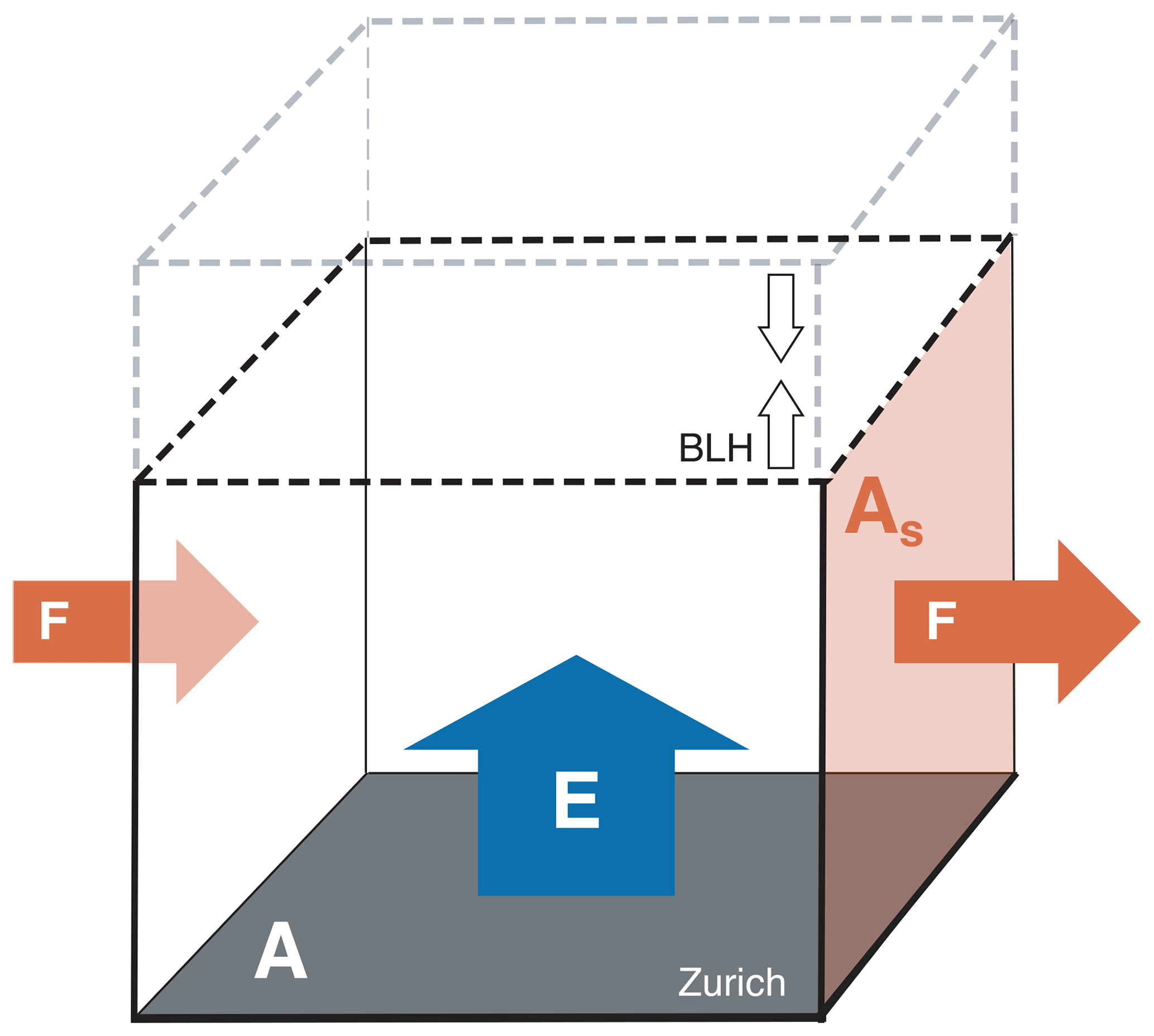
Figure 1Box model used to estimate GEM emissions E of Zurich. A represents the area of the base and A_s the area of the lateral side of the box. The variable boundary-layer height (BLH) determines the height of the box and F the advective flow.

Download

2.3 Model parametrization

Over the course of the measurement period, nine episodes of day–night inversion were identified by visual inspection for the criteria of strong day–night inversion. Only events lasting for a minimum of 4 days were considered. Individual periods show a considerably longer duration of up to 14 days. These events are then reproduced with our previously developed and validated model. While in our previous studies the temporal resolution of the air monitoring was significantly limited (resolution of hours to weeks), we profit here from highly resolved GEM data (5 min resolution). We follow the approach to strip the model to the minimum, and only processes indispensable to the parametrization of the conditions at hand are incorporated. This lean model approach prevents over-interpretation of model results and the reduced complexity provides a better conceivability of the model. Thereby, we end up with a model consisting of a single box of air that covers an area A of 10 km × 10 km (100 km²) approximating Zurich's size inhabited by roughly 400 000 people (Fig. 1). The box size was chosen to encompass the city's emission sources and has proven to be suitable by previous studies (Wang et al., 2012; Buser et al., 2013; Bogdal et al., 2014b). Based on the national emission inventory (Heldstab et al., 2015), half of the mercury emissions are assumed to stem from mixed sources such as stationary combustion, minor industrial activities and houses distributed all over the city. The other half is assumed to come from a municipal waste incineration plant in the middle of the city, where a chimney (height 90 m) leads to a broader distribution. For Zurich this shows an emission profile similar to unintentional combustion byproducts such as polychlorinated dibenzo-p-dioxins and dibenzofurans studied in the work of Bogdal et al. (2014b). Since for this study on GEM we only have one measurement location at near surface level, the assumption of a homogeneously mixed air compartment below the nocturnal boundary layer is necessary. The previous studies on dioxins have shown that this assumption is justifiable. Possible stratification, however, remains a source of uncertainty in our model. Emissions of oxidized mercury species such as HgCl₂ as well as particulate mercury were not included in the model. Regarding the local emissions of oxidized mercury, we did not have any data available. The only major source would be the municipal waste incineration plant. Considering the flue-gas treatment systems installed, however, we assume stack emissions to be predominantly in the form of GEM (van Velzen et al., 2002). Flue gas is treated with an ESP, SCR, AC, and three-step WFGD, in this order. (ESP: electrostatic precipitator, SCR: selective catalytic reduction, AC: activated carbon injection, WFGD: wet flue-gas desulfurization). Regarding the GEM ∕ GOM ratio the effect of flue-gas treatment on mercury emissions is, however, still unclear, leaving some level of uncertainty to our assumption (Zhang et al., 2016). Mercury emissions stemming from reduction of oxidized mercury reservoirs are thus contained in the total GEM emission estimates.

The time-dependent parameters included in the model are (i) the boundary-layer height (BLH), defining the volume of the box; (ii) the wind speed to model advective flux (F) through the box; and (iii) the background concentrations to quantify the concentrations of the advective flux.

The model is operated dynamically with an hourly resolution. Due to the small size of the model area, many parameters usually included in box models can be disregarded. Slow processes such as deposition to soil and water, as well as re-emission from these compartments, are negligible. Atmospheric oxidation of GEM to GOM is excluded as well due to the short residence time of mercury within the considered small model region (less than 1 h for wind speed of 3 m s⁻¹). Our own calculations, with a version including atmospheric degradation reactions, show that losses by degradation are negligible in comparison to the advective fluxes.

The focus of the model is on the emission flux, which is directed to the surface air compartment and is kept constant over the course of an inversion period. The goal is to find the emission term that results in a modeled surface GEM concentration best matching the measured concentrations. The emission flux is the only adjustable parameter in the model, whereas all further model parameters are preset and not adapted to improve the fit between model results and field measurements. The root mean square error (RMSE) is used as a measure for optimization in an iterative fitting process. The emission flux resulting in the lowest RMSE is then applied as the city's source term.

2.3.1 Model setup

The model includes the following three time-dependent model parameters.

• i.

  The boundary-layer height (BLH) is used as a measure to define the volumes of the air compartment of the model (Fig. 1). In a first model approach, boundary-layer heights are approximated using constant levels for the daylight and nightly period. The height is set to 1500 m for the convective boundary layer (CBL) during the day from 08:00 (UTC+1) until 20:00 and lowered to 150 m for the nocturnal boundary layer (NBL) at 21:00. The NBL level is based on common meteorological conditions (Stull, 1988) and our own experiences in previous work (MacLeod et al., 2007; Gasic et al., 2009; Wang et al., 2012; Buser et al., 2013; Bogdal et al., 2014b). A sharp transition is used between NBL and CBL. These heights determine the box volume of the air layer. Changes in the volume of the air compartment are handled such that, in cases of a decline in BLH, the amount of GEM in the volume difference is transferred out of the box. In cases of a rise in the BLH, the GEM concentration in the air compartment is diluted with the corresponding air volume with GEM concentration of background levels.

• ii.

  The advection is determined by the wind speed. Wind speed measurements are conducted above a roof top (33 m a.g.l.). Studies by Benz (1988) and Schuhmacher (1992) in Zurich show that measurements at this height are representative for the mean wind speed for the height profile from 0 to 150 m. As shown later only nightly periods where the BLH is 150 m are relevant to estimate emissions in Zurich. Wind direction is not taken into consideration. Therefore, advection F is always occurring through a lateral face of the box (Fig. 1) and the flux is obtained by multiplication of its area A_s with the corresponding wind speed u, $F=A_{\text{s}}\cdot u$.

• iii.

  The background concentration is set to a steady level of 1.5 ng m⁻³. It lies in the lower 10 % quantile of the whole 2-year measurement series in Zurich and no adaption was made for nightly backgrounds. In reality, background concentrations are likely to be higher than this level since also at high wind speeds measurements rarely fall below as we show in Figs. S1 and S2 in the Supplement. The value of 1.5 ng m⁻³ lies in the range of what we measured at the outskirts of the city of Zurich (Zurich zoo, median = 1.62 ng m⁻³, Q_0.1=1.53 ng m⁻³, Q_0.9=1.77 ng m⁻³). On the basis of this assumption an upper-bound model run regarding the source strength of the city is calculated. To establish a margin, which restricts the source strength with a realistic lower-bound, background concentrations are raised to the median concentration of 1.8 ng m⁻³ for a second emission estimate. We are confident that actual emissions reside within the range of these two model runs.

Figure 2Comparison between normalized GEM, CH₄ and CO levels (divided by overall mean) showing the temporal variation over a weekly, daily, monthly and weekday course. Mean values and 95 % confidence intervals are shown. Source: NABEL (FOEN and Empa; BAFU/EMPA, 2018).

Download

3.1 Measurement series

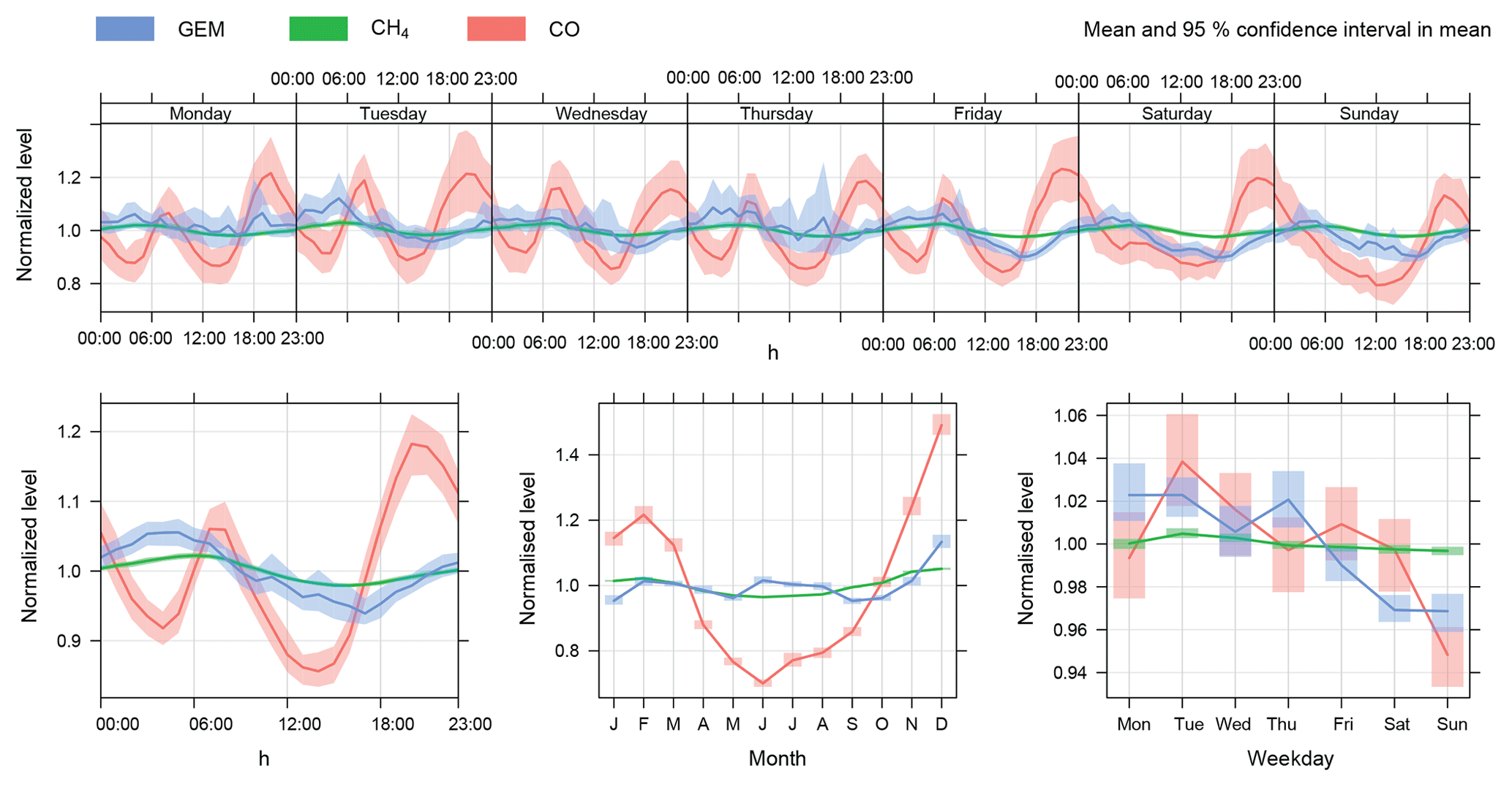
GEM levels measured in Zurich from December 2013 until December 2015 show a median concentration of 1.81 ng m⁻³ (Q_0.1=1.55 ng m⁻³, Q_0.9=2.36 ng m⁻³). The concentration gradient for GEM follows a weak diurnal pattern, similar to CH₄ concentrations, however, with a more prominent amplitude. Figure 2 shows the diurnal pattern of GEM, CH₄ (i.e. conservative tracer) and CO (i.e. combustion indicator) measurements normalized by their respective mean concentration. The rise in concentrations during nighttime and the minimal concentrations during the afternoon are anti-cyclical to the wind speed and suggest a meteorological cause for the pattern. Stable conditions with lower wind speeds and lower boundary-layer height during the night lead to a slight concentration rise, while higher thermal convection during daytime lower these concentrations. The wind rose plots (Fig. S3) for GEM, CH₄ and CO support these findings and our initial hypothesis of a constant source term of GEM for the city. GEM concentrations are thus primarily influenced by the wind speed and the diluting effect of lower background concentrations (Fig. S2). However, one can also observe slightly lower GEM concentration towards the weekend, with the lowest concentrations on Sundays (Fig. 2). More prominently this is the case for CO, which has sources that are strongly activity-related, such as traffic. We therefore deduce that besides the prominent constant sources for GEM, there are also activity-related emissions but of a much smaller scale. The inversion events for the summer extracted from the measurement series show a clear diurnal trend not only for GEM but also for CH₄ (Fig. S4); both trace gases stem from constant sources. In winter inversion periods concentrations for PM₁₀, CO, SO₂ and NO_x also follow the course of GEM since combustion-related sources have a more constant source term (Fig. S5). These comparisons indicate that the emission flux for GEM and CH₄ are constant over time.

For the measurement series at Zurich zoo on the outskirts of the city, a median GEM concentration of 1.62 ng m⁻³ (Q_0.1=1.53 ng m⁻³, Q_0.9=1.77 ng m⁻³) was obtained. GEM levels are significantly lower and the concentration range is much smaller at this measurement site – a clear indicator that this location is much less affected by local sources. Furthermore, these results confirm the assumption that background air is lower in concentration and suggest that background concentrations at a level of 1.5 ng m⁻³ are in fact a lower-bound estimate.

Figure 3Example period from 24 June until 6 July 2015 that shows a day–night pattern for ground inversion. (a) shows the boundary-layer heights for the basic scenario (orange). (b) shows the wind speed (ws). (c) shows GEM measurements in blue and the basic model results in orange.

Download

3.2 Boundary-layer budget

To illustrate the model results, we present the period showing longest continuing day–night inversion from 24 June until 6 July 2015 (Fig. 3) as an example. Analogous figures for the other eight inversion periods are shown in the Supplement (Figs. S6–S14). Figure 3 shows the most important model parameters: Fig. 3a shows the boundary-layer height, Fig. 3b shows the wind speed, and Fig. 3c shows the measured GEM concentrations (blue) and the model results (orange). GEM measurements show a clear diurnal variation with high concentrations of up to more than 3 ng m⁻³ during the night and lower concentrations during the day. The model results follow this pattern. The emissions strength of the city is observable from the steep concentration increase, when the BLH is lowered. These nocturnal periods with low wind speeds (<2 m s⁻¹) are used to estimate the source term of the city. During daytime the modeled concentrations are dominated almost entirely by the background concentrations due to the higher BLH and the stronger wind speeds, which create a much bigger flux than the city's GEM emissions.

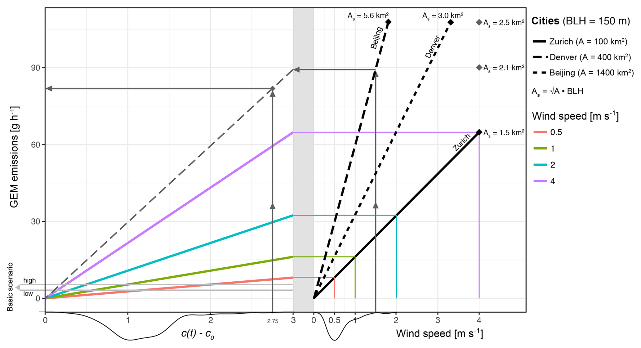
Figure 4Graphical representation of the steady-state formula $E=u\cdot A_{\text{s}}\cdot (c-c_{\text{back}})$ to estimate emissions in a box model. Starting at different wind speeds, the colors show the corresponding GEM emission estimate for Zurich in relation to the concentration difference between measurement c and background c₀. The results of the basic emission scenario are given as gray lines. The gray shading highlights the range in concentration differences obtained in Zurich. An example of how emissions are estimated for another city is given for Beijing, with a wind speed of 1.5 m s⁻¹ and 2.6 ng m⁻³ concentration difference.

Download

Table 1The emission estimates of GEM in Zurich, Switzerland, are shown for all nine observed summer periods.

Download Print Version | Download XLSX

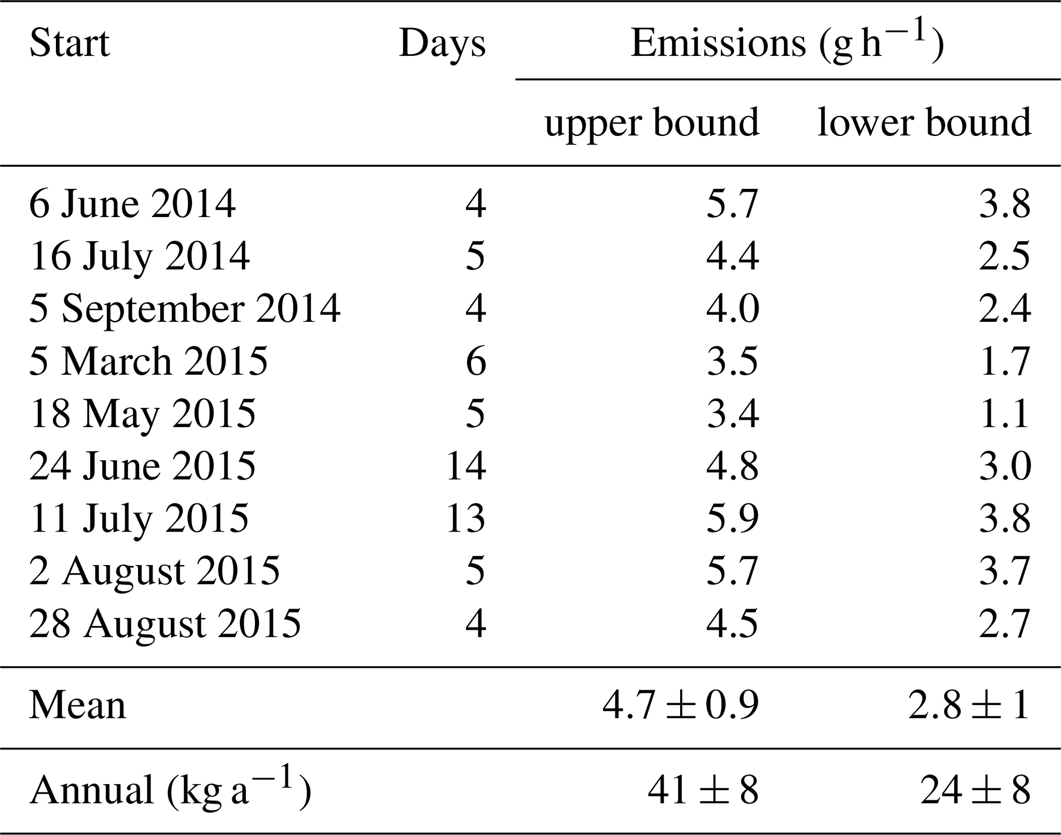
In general, model results follow the measured concentration, suggesting advection and boundary-layer height are indeed enough to describe most of the GEM variation. During daytime, model results are slightly lower than measured GEM levels, showing that our model approach covers the most important atmospheric processes occurring on this timescale and successfully reproduces the fate of GEM in the urban air of Zurich. Using RMSE reduction we find a GEM emission flux of 4.8 g h⁻¹ (Table 1) for the modeled region in this period, or 42 kg a⁻¹ when extrapolated to annual emissions for the city of Zurich. Over all nine periods, we find a mean emission of 4.7±0.9 g h⁻¹ or 41±8 kg a⁻¹ (Table 1). The low variance of the emission estimate over all the nine periods from different months and years supports our claim of a constant mercury emission term for the city. Also for three winter periods with long stable inversion conditions (Figs. S15–S17) emission estimates in the same range are observed (4.4±0.8 g h⁻¹; see Table S1 in the Supplement).

3.2.1 Uncertainties of the emission estimates

The mass balance for mercury in the air compartment of the box (m) is formulated as follows:

$$\begin{array}{}\text{(1)}& {\displaystyle \frac{\mathrm{d}m}{\mathrm{d}t}}& {\displaystyle }=V\cdot {\displaystyle \frac{\mathrm{d}c}{\mathrm{d}t}}=F_{\text{adv}}\cdot c_{\text{back}}-F_{\text{adv}}\cdot c\left(t\right)+E,\text{(2)}& {\displaystyle \frac{\mathrm{d}m}{\mathrm{d}t}}& {\displaystyle }=u\cdot A_{\text{s}}\cdot c_{\text{back}}-u\cdot A_{\text{s}}\cdot c\left(t\right)+E,\end{array}$$

where V (m³) is the volume of the box, c_back is the background concentration (ng m⁻³) and E is the emission flux (g s⁻³). The advective air flux F_adv (m³ s⁻¹) is calculated from the wind with velocity u (m s⁻¹) that flows through the lateral side of the box A_s (m²). Although the emission estimations presented so far are based on a dynamic time-resolved box model, we introduce here the steady-state case for the sake of simplification. For the steady-state solution ($\frac{\mathrm{d}m}{\mathrm{d}t}=\mathrm{0}$) the emission flux is $E=u\cdot A_{\text{s}}\cdot (c-c_{\text{back}})$. The problems at hand are of a linear nature. Therefore, error handling is straightforward and the maximum error bound could be found using linear error propagation (MacLeod et al., 2002), and a given uncertainty in a parameter would at worst results in an equal uncertainty in the model result. However, the true errors of the parameters are unknown and not all of them would strictly follow a known distribution. The procedure we apply here leads to a more confident error margin.

As mentioned before, the background concentration, c_back, of 1.5 ng m⁻³ used until now is a lower bound for the background concentration that leads to an upper-bound estimate for the true GEM emissions. By using 1.8 ng m⁻³ as background concentration (+20 %), which is equal to the median and a high estimate for the background, we are able to set a lower bound for emissions. These two margins are more helpful in the error characterization than a technical error-propagation approach. Following this approach we obtain a lower-bound emission of 2.8±1.0 g h⁻¹ (Table 1, mean of the lower-bound scenarios of the nine periods ± standard deviation) and can thereby narrow down the true GEM emissions for Zurich. According to our findings they must amount to a value between 2.8±1.0 and 4.7±0.9 g h⁻¹. In this range we also see the sensitivity of the background concentration for the model results. As shown, a change in c_back by 20 % resulted in a mean emission estimate for all nine periods lower by 40 %. The sensitivity ($S=(\mathrm{\Delta }O/O)/(\mathrm{\Delta }I/I)$, MacLeod et al., 2002) of c_back (I) regarding the mean emission estimate (O) amounts to S=2.

After the background concentration, the BLH is the most sensitive parameter. An increase in the BLH by 10 % results in an equally larger emission estimate: S for the BLH equals 1. As mentioned before the height of 150 m for Zurich has been established in previous model studies from temperature profiles. To test this value and the assumption of a constant height, we established an advanced model scenario, where the BLH is derived from a complex numerical weather prediction model (COSMO-2), developed by MeteoSwiss. The BLH is determined both for day and night with an hourly time resolution. The approach for the advanced scenario is presented in detail in the Supplement. All model runs of the advanced scenario are displayed in Figs. S6–S14. The emission estimates based on this advanced approach (4.9±1.7 g h⁻¹, Table S1) are very close to the basic scenario with the fixed BLH presented here (4.7±0.9 g h⁻¹). Additionally, the advanced model often does not provide a better model fit than the RMSE comparison show in Table S1. On this basis and in accordance with the outcome of the two model approaches, we favor the basic approach with a fixed BLH of 150 m. The reason being that we can thereby reduce model complexity, which is not necessary to adequately describe the situation at hand.

Other important model parameters to be discussed here are the model area with a sensitivity of S=0.6 and the wind speed with a sensitivity of S=0.4. If we again look at a steady-state example ($\frac{\mathrm{d}m}{\mathrm{d}t}=\mathrm{0}$) of Eq. (2) and rearrange to $c=c_{\text{back}}+E/(u\cdot A_{\text{s}})$, we see that the ratio between the emission flux E and the advective flux (u⋅A_s) determines the deviation of the concentration from the background concentration c−c_back. During the day, advective fluxes are much larger than the emission term we estimate for Zurich. For the small box in Zurich even for very low wind speeds of 1 m s⁻¹, F_adv is 7 times bigger than E. Therefore, c is dominated by c_back during the day in our model. The explanatory power of the model is much stronger during the nocturnal inversion periods with low BLH and low wind speeds. During these periods advection has little influence. The model application domain for the two cases of high and low BLH are displayed in Fig. S18. These curves set the domain regarding the GEM concentrations explainable by our model depending on the BLH, the wind speed and the model area. The model area has to be chosen to encompass all important sources and be big enough to allow for a reasonable time step in the model setup. For large model areas, however, inhomogeneities in the model region could be problematic. Here, we assume homogeneous distribution of GEM in our model region of 10 km by 10 km. As work by Cairns et al. (2011) shows, GEM concentrations in Toronto do follow a certain distribution and differences in concentrations do occur depending on the measurement location. Our measurement site has been assessed for pollutants with diffuse emissions with passive samplers by comparing various sites throughout the city. The location proved to be a representative study site for an anthropogenic pollutant with diffuse emissions (Diefenbacher et al., 2015b, 2016). As mentioned before, mercury emissions in Zurich stem from diffuse sources, which are distributed in the whole city and a waste incineration plant in the city center. Emission estimates derived with our box model only apply to the whole city or can be averaged by person. Spatially resolved emission estimates are, however, not attainable.

The comparison of GEM measurements to CO and CH₄ levels (see Figs. 2, S4 and S5) strongly suggests that GEM emissions in Zurich largely stem from constant sources. Activity-related emissions, i.e. from traffic, are a minor contributor. Also, from the comparison between summer and winter periods, which are comparable in terms of emission strength, we conclude that the increased combustion activities during the cold winter months are not a large contributor to overall GEM emissions. Possibly, increased GEM emissions from enhanced combustion activities in winter are compensated for by reduced emissions of GEM by evaporation from legacy mercury reservoirs in periods with low ambient temperatures and vice versa in winter.

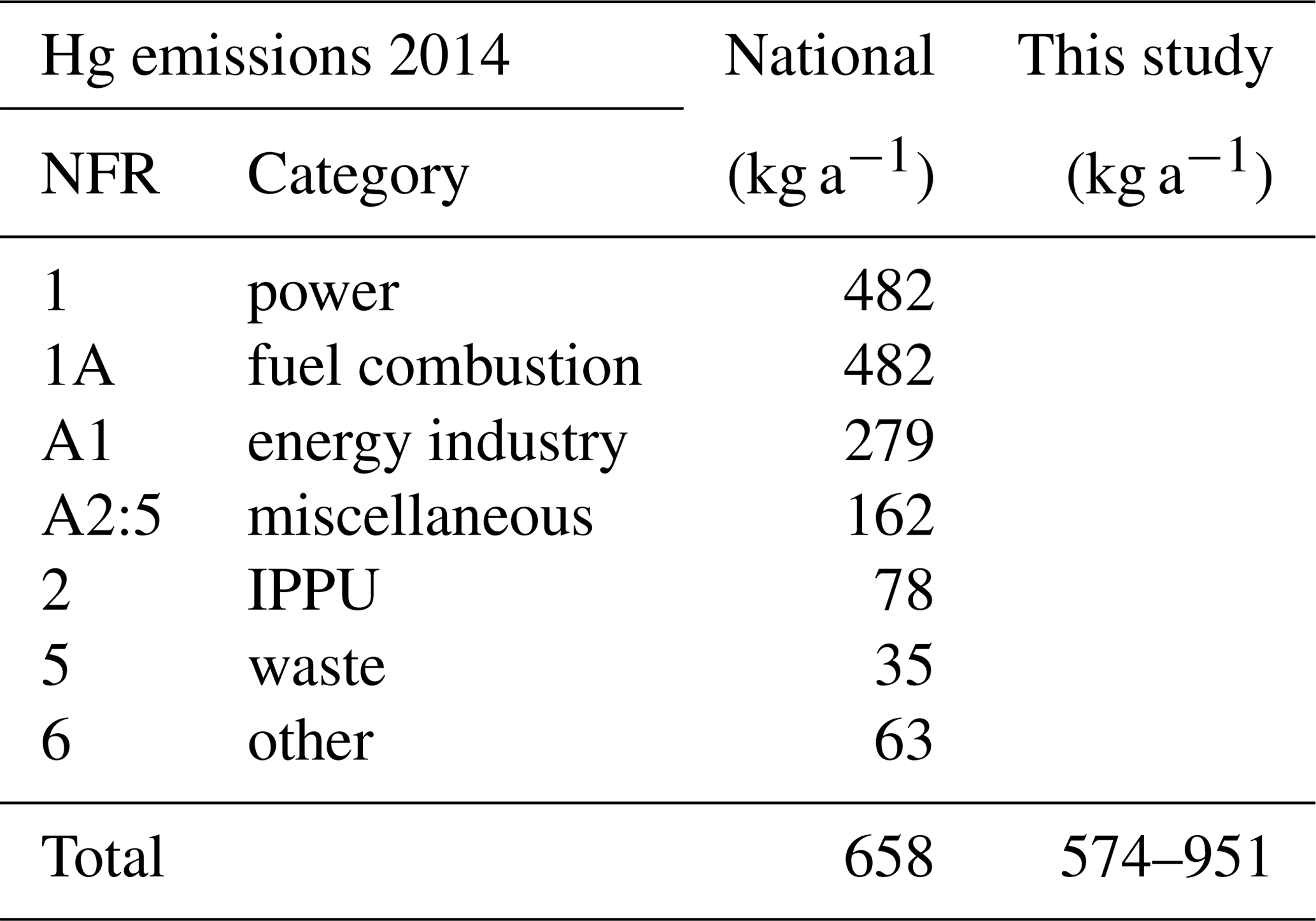
Table 2Swiss national inventory for mercury emissions in 2014 as submitted under the UNECE Convention on Long-Range Transboundary Air Pollution. (NFR: nomenclature for reporting emission categories, IPPU: industrial processes and product use).

Download Print Version | Download XLSX

3.3 Implication on emission reporting

Mercury emissions are annually reported by countries signatories to the Protocol on Heavy Metals to the UNECE Convention on Long-Range Transboundary Air Pollution (CLRTP). Swiss national CLRTP inventories for mercury emissions to the atmosphere reported a total of 658 kg a⁻¹ for the year 2014 (Heldstab et al., 2015). Mercury emissions are not differentiated by species: GEM or GOM. Due to the lack of these data we are forced to work with assumptions. Considering the nature of emission sources and relatively strict regulation on stack emissions, we assume all emissions to be in the form of GEM. The biggest share, 73 % of the emissions, stems from the energy sector (1A1), of which the majority is allocated to energy industries for public electricity and heat production. The main sources to this energy sector are waste incineration plants. In Switzerland energy recovery from municipal solid waste incineration is mandatory and emissions from waste incineration plants are reported under this category. Other combustion processes mainly in manufacturing industries (1A2:5) make up 25 % of the total emissions. These numbers and categorization into individual sectors and subcategories as shown in Table 2 and set the basis for the allocation to the global emission grid of the European Monitoring and Evaluation Programme (EMEP) for Switzerland. The grid shows spatially resolved emissions with a $\mathrm{0.1}{}^{\circ }\times \mathrm{0.1}{}^{\circ }$ (approx. 10 km × 10 km) resolution. The allocation rules for the emissions rely mostly on population density and vary from one source category to another. Depending on the source category, different weightings on the prevailing employment sectors are installed. For Zurich, the gridded emissions report an emission flux of 18 kg for the year 2014 (18 kg for 2015). Our boundary-layer budget approach results in a GEM emission flux between 24 and 41 kg for Zurich. These findings suggest emission of about double the amount allocated to Zurich by the rule set for the EMEP report. If we were to apply the same allocation factors to the model results we would come up with national GEM emission of 934 to 1581 kg a⁻¹, i.e. clearly higher than reported by the authorities. When we use population data only as a criterion, a scaling factor of 20.5 would be appropriate, considering a population of approximately 400 000 residents in the modeled area and a Swiss population of 8.2 million people. This approach would amount to emission of 494 to 837 kg GEM per year. In comparison to the 658 kg a⁻¹ of the Swiss CLRTP report, these results lie in a very acceptable range and show that the approach explained here can be used to validate national reporting. Moreover, from our results we suggest that the allocation formula for mercury for the EMEP grid should be adjusted such that population data are given more weight over other parameters. For Zurich we find a per capita emission of 0.06 to 0.10 g a⁻¹ per person. This estimate is somewhat lower than the European per capita emission of 0.19 g a⁻¹ reported in the AMAP/UNEP (2013) background report.