the Creative Commons Attribution 4.0 License.
the Creative Commons Attribution 4.0 License.
 | 25 Mar 2019
Photochemistry on the bottom side of the mesospheric Na layer
Wuhu Feng
John M. C. Plane
Daniel R. Marsh
Lidar observations of the mesospheric Na layer have revealed considerable diurnal variations, particularly on the bottom side of the layer, where more than an order-of-magnitude increase in Na density has been observed below 80 km after sunrise. In this paper, multi-year Na lidar observations are utilized over a full diurnal cycle at Utah State University (USU) (41.8∘ N, 111.8∘ W) and a global atmospheric model of Na with 0.5 km vertical resolution in the mesosphere and lower thermosphere (WACCM-Na) to explore the dramatic changes of Na density on the bottom side of the layer. Photolysis of the principal reservoir NaHCO3 is shown to be primarily responsible for the increase in Na after sunrise, amplified by the increased rate of reaction of NaHCO3 with atomic H, which is mainly produced from the photolysis of H2O and the reaction of OH with O3. This finding is further supported by Na lidar observation at USU during the solar eclipse (>96 % totality) event on 21 August 2017, when a decrease and recovery of the Na density on the bottom side of the layer were observed. Lastly, the model simulation shows that the Fe density below around 80 km increases more strongly and earlier than observed Na changes during sunrise because of the considerably faster photolysis rate of its major reservoir of FeOH.
- Article
(5384 KB) - Full-text XML
- BibTeX
- EndNote


The layer of Na atoms in the upper mesosphere and lower thermosphere (MLT, ∼80–105 km in altitude) is formed naturally by meteoric ablation along with other metallic layers such as Fe, Mg, Ca and K (Plane et al., 2015). The climatological variations of this Na layer are known to be mainly controlled by a series of chemical reactions and dynamics, including tides, gravity waves and the mean circulation in the MLT (Plane, 2004; Marsh et al., 2013). Mesospheric Na atoms are an important tracer in the MLT, where they are observed by resonance fluorescence, either by the lidar technique (Krueger et al., 2015) or solar-pumped dayglow from space (Fan et al., 2007). The Na lidar technique has enabled high temporal and spatial resolution measurements of the mesospheric Na layer since the 1970s (Sandford and Gibson, 1970). In addition to Na density observations, Na temperature/wind lidars can measure the atmospheric temperature and wind fields over the full diurnal cycle by observing Doppler broadening and shifting of the hyperfine structure of one of the Na D lines (Krueger et al., 2015). Atmospheric observations have been complemented by laboratory kinetic studies of the important reactions which control both the neutral and ion-molecule chemistry of Na in the MLT (Plane, 1999, 2004; Plane et al., 2014, 2015), and the development of atmospheric models which satisfactorily reproduce seasonal observations over most latitudes (Plane, 2004; Marsh et al., 2013; Li et al., 2018).
However, less detailed work has been done to investigate the diurnal variations in Na density, especially on the bottom side of the layer where neutral chemistry dominates. Advances in lidar technology have enabled Na density observations over a full diurnal cycle (Chen et al., 1996; States and Gardner, 1999; Clemesha et al., 2002; Yuan et al., 2012). Utilizing multi-year observations, Yuan et al. (2012) investigated the diurnal variation and tidal period perturbations of the Na density. These tidal Na perturbations were then used to estimate the tidal vertical wind perturbations (Yuan et al., 2014), showing that, although closely correlated with tidal waves and dominated by tidal wave modulations in the lower thermosphere, the Na diurnal and semidiurnal variations cannot be induced by tidal modulations alone. This is especially the case on the bottom side of the layer below ∼90 km, where tidal wave amplitudes are relatively small (see Fig. 5a and b in Yuan et al., 2012), implying that other mechanisms make a significant contribution to the diurnal variation in the Na bottom side of the layer.
Plane et al. (1999) recognized the important role of photochemical reactions for characterizing the bottom side of the Na layer and then measured the photolysis cross sections of several Na-containing molecules – NaO, NaO2, NaOH and NaHCO3, which models show to be significant mesospheric reservoir species (Self and Plane, 2002; Marsh et al., 2013). These cross sections, measured at temperatures appropriate to the MLT, were then used to calculate mesospheric photolysis rates:
These direct photochemical reactions release atomic Na during the daytime. Furthermore, indirect photochemistry also plays a role. The photolysis of O2, O3 and H2O (Brasseur and Solomon, 2005) leads to the production of H and O (R5–R8), increasing their concentrations by more than 1 order of magnitude during the daytime at an altitude around 80 km (Plane, 2003). The daily variation in H is further facilitated by the reactions between HO2 and O∕O3, which has strong diurnal variations.
Thus, H and O reduce the Na compounds listed above to atomic Na (Plane, 2004).
To demonstrate the effect of solar radiation on the mesospheric Na layer, including (R1)–(R8), Fig. 1 shows the averaged Na density variation in the layer between 75 and 105 km during a 6 h period that straddles sunrise (from 3 h before to 3 h after sunrise) in the fall season (from 20 August to 30 September). The results are based on 50 days of Na lidar observations at USU (41.8∘ N, 111.8∘ W) between 2011 and 2016. Figure 1 also includes the ratio profile between the Na density 3 h after sunrise to that 3 h before sunrise. The lidar observations clearly show that, while there is an overall Na density increase after sunrise below ∼92 km, the increase at and below 80 km is much larger than closer to the layer peak: the Na density increases by a factor of ∼6 at 80 km and ∼40 near 78 km, whereas it is almost unchanged around ∼95 km. The dramatic oscillation of the ratio below 78 km is due to very low Na density before sunrise (usually below 1 cm−3). Note that this ratio calculation for Na density profiles 1 h before and 1 h after sunrise generates a similar ratio profile, which demonstrated an even larger ratio near 80 km, a factor of ∼20. This implies a very quick Na density enhancement during sunrise. This analysis therefore provides strong evidence of the impact of photochemistry on the bottom side of the Na layer.
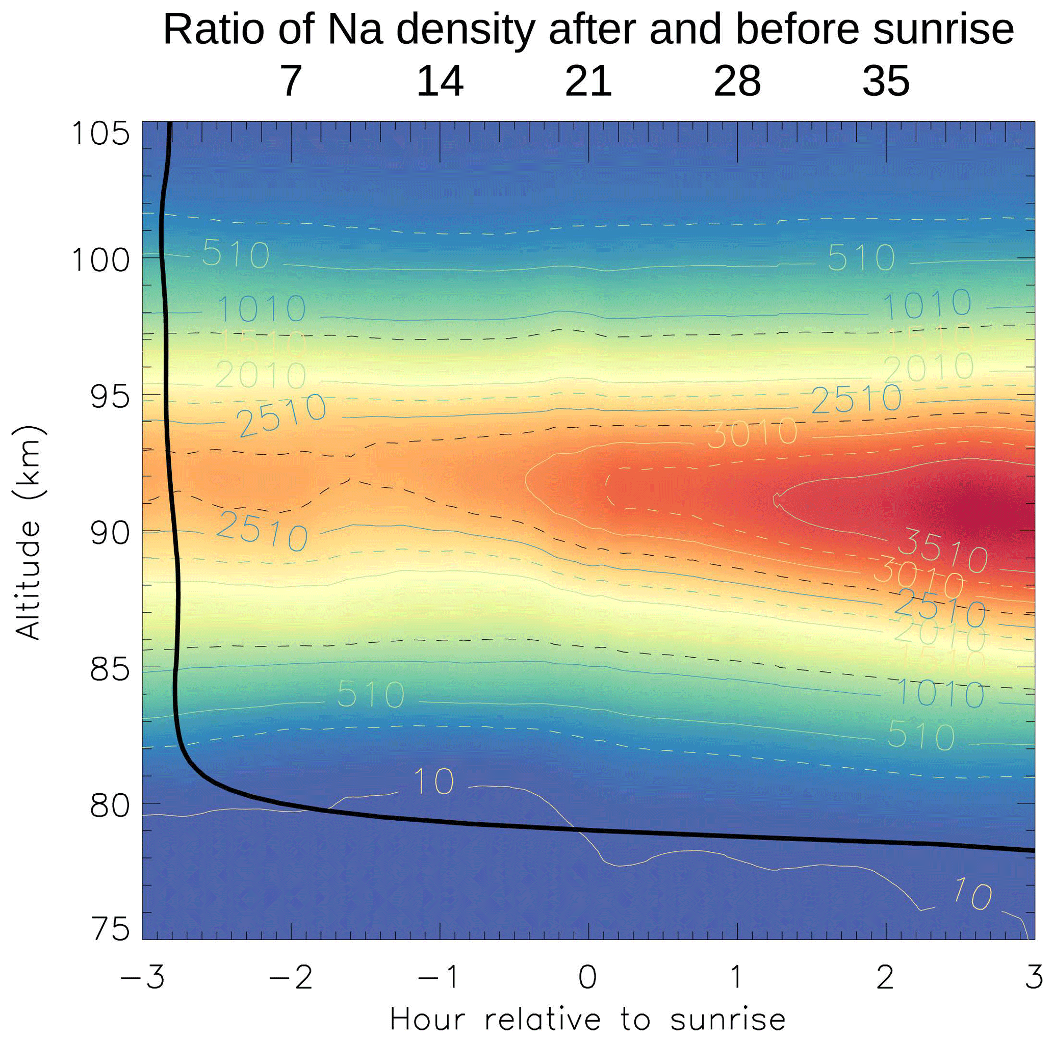
Figure 1The Na density (cm−3) variation between 75 and 105 km in MLT during sunrise between 20 August and 30 September (contour) in 2011–2016. Zero hour marks time of the sunrise at the mesopause (bottom abscissa). The solid black profile is the ratio between the Na density 3 h after sunrise to that 3 h before sunrise (its tick marks is plotted in the top abscissa).
In this paper we compare the USU Na lidar diurnal cycle observations of the mesospheric Na layer during a continuous 7-day campaign in fall 2012 with the Na density variation simulated by NCAR's Whole Atmosphere Community Climate Model with Na chemistry (WACCM-Na) (Marsh et al., 2013) for the USU location during the same period, in order to quantitatively investigate the role of photochemistry on the Na layer. In addition, Fe density variation by the latest WACCM-Fe (Feng et al., 2017) due to photolysis is also discussed to show the distinct feature of the Fe in the bottom side of the main layer. The Na lidar measurements made during the solar eclipse on 21 August 2017 in North America are then used as a further robust test of the role of photolysis.
The USU Na temperature–wind lidar system, originally developed at Colorado State University, has been operating at the USU main campus since summer 2010. In addition to Na density observations, neutral temperature and winds are also measured for the mesopause region (∼80–110 km) (Krueger et al., 2015). The lidar return signals can be recorded in 150 m bins in the line-of-sight direction and saved every minute. Facilitated by a pair of customized Faraday filters deployed at its receiver (Harrell et al., 2009), this advanced lidar system can also reject the sky background significantly during the daytime while receiving the Na echo with minimum loss. This technique provides robust measurements of these important atmospheric parameters under sunlight conditions, thereby enabling this investigation of Na photochemistry. In this study, we focus on two sets of Na lidar data: Na density data taken between UT Day 271 (27 September) and UT Day 277 (3 October) of 2012 and lidar observations during the solar eclipse on 21 August 2017. The lidar observations presented here are processed with 2 km vertical resolution, and 10 and 30 min temporal resolution for nighttime and daytime data, respectively, to achieve appropriate signal to noise (S∕N) for studying the bottom side of the layer between 75 and 80 km, where the Na density is low (<100 cm−3). The standard deviation of the Na number density is ∼10 % to 40 % between 85 and 95 km during this 7-day campaign. The lidar observations during the solar eclipse are processed with 10 min resolution to investigate the potential eclipse-induced perturbations in detail.
WACCM-Na is a global meteoric Na model which satisfactorily reproduces lidar and satellite measurements of the Na layer (e.g., Marsh et al., 2013; Dunker et al., 2015; Plane et al., 2015; Langowski et al., 2017; Dawkins et al., 2016; Feng et al., 2017). WACCM-Na uses the Community Earth System Model (version 1) framework (e.g., Hurrell et al., 2013), which includes detailed physical processes as described in the Community Atmosphere Model, version 4 (CAM4) (Neale et al., 2012), and has the fully interactive chemistry described in Kinnison et al. (2007). The current configuration for WACCM is based on a finite volume dynamical core (Lin, 2004) for tracer advection. Water vapor in WACCM is prognostic and includes the source in the stratosphere from methane oxidation. The approximate water vapor concentration at the USU Na lidar site between 75 and 80 km on the day of the eclipse is 1–3×109 cm−3 (equivalent to 3–5 ppmv). For the present study, we used a specific dynamics (SD) version of WACCM, in which winds and temperatures below 50–60 km are nudged towards NASA's Modern-Era Retrospective analysis for Research and Applications (MERRA) (Lamarque et al., 2012). The horizontal resolution is 1.9∘ latitude × 2.5∘ longitude. For this study we performed model experiments using two different vertical resolutions: 88 and 144 vertical model levels (termed as lev88 and lev144), both of which have the same 62 vertical levels from the surface to 0.42 Pa (below ∼50 km) as MERRA with different vertical resolutions above 0.42 Pa. Basically, lev88, which has been used as a standard SD-WACCM, gives a coarse height resolution from ∼1.9 to ∼3.5 km above the upper stratosphere to MLT, while lev144 increases the resolution from 1.9 km down to around 500 m in the MLT (Merkel et al., 2009; Viehl et al., 2016). The Na reaction scheme described in Plane et al. (2015) is updated with the results of recent laboratory studies (Gómez-Martín et al., 2016, 2017), and the meteoric input function (MIF) of Na from Carrillo-Sánchez et al. (2016) is used. Note that the absolute Na MIF used in this paper is the same as in Li et al. (2018) and Plane et al. (2018); i.e., it has been divided by a factor of 5 from the MIF in Cárrillo-Sanchez et al. (2016), to match the observations. In order to contrast the photochemical behavior of the Na bottom side of the layer with that of the Fe layer, a WACCM-Fe simulation was also performed. The model output was sampled over USU (41.8∘ N, 111.8∘ W) every 30 min (the model time step), then interpolated to the same observational period for the available lidar daytime measurements for direct comparisons. Note that the modeled nighttime outputs use the same temporal resolution as that of the daytime results because the model time step is every 30 min, while the lidar nighttime measurement is every 10 min.
The averaged Na density diurnal variation calculated from the intensive 7-day USU Na lidar campaign is presented in Fig. 2a. During the campaign, the time of sunrise in the MLT is around 06:56 local time (LT) based on solar elevation angle (−5∘ represents sunrise in the MLT); the noon and sunset times are 13:45 and 20:35 LT, respectively. The observations reveal strong variations within the layer during the day. Close to the layer peak there are three minima at around 20:00 LT (evening), 04:00 LT (right before dawn) and 16:00 LT (afternoon), where the Na density falls to ∼3000 cm−3. These are separated by two significant maxima near 91 km: the stronger one occurs right after sunrise and lasts almost the whole morning with a peak density more than 4400 cm−3; the other maximum occurs near 22:00 LT (shortly before midnight), and has a much shorter lifetime (∼1 h) with peak density slightly above 4100 cm−3. Similarly to Fig. 1, on the bottom side of the main layer there is clear evidence of an increase in Na density after sunrise.
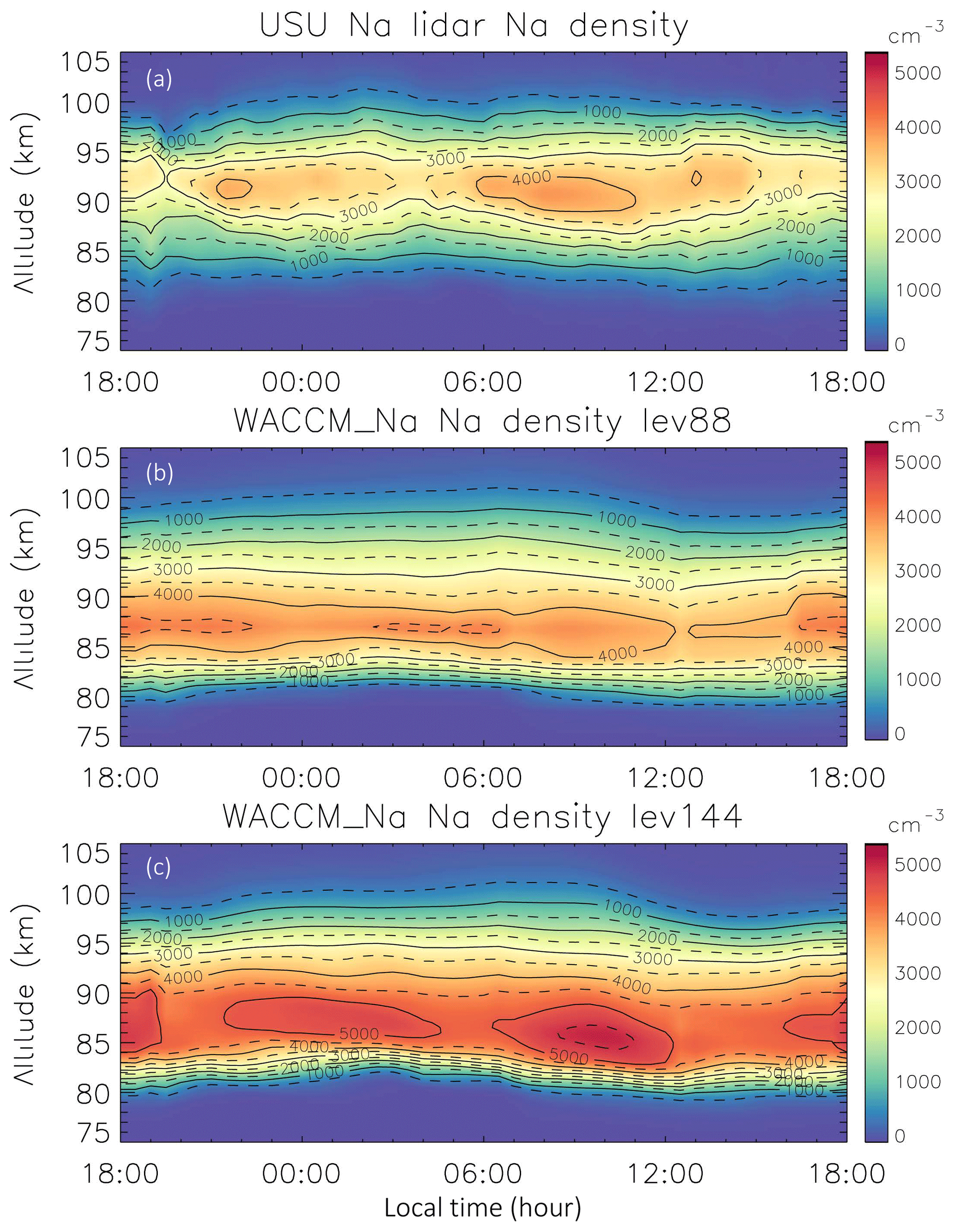
Figure 2The averaged lidar measured Na density variation during the 7-day Na lidar campaign between 27 September and 3 October 2012 (a); the Na density variations at USU locations during the same time frame, simulated by WACCM_Na 88-level (b) and 144-level (c).
Compared with the lidar observations, Fig. 2b shows that the relatively coarse-resolution WACCM-Na produces a reasonable Na layer in terms of a peak Na density close to 4500 cm−3. However, in contrast to the lidar observations, three distinct features are observed: first, the maxima and minima around the layer peak are much less obvious; second, the peak height of the simulated Na layer is near 87 km, about 3–4 km lower than the lidar observations, partly due to the mesopause in SD-WACCM, which is a few kilometers lower (Feng et al., 2013); third, the absolute value of the Na density vertical gradient below the layer peak is much larger than observed. For instance, the modeled Na density decreases from near 4500 cm−3 at 87 km to ∼2000 cm−3 around 82 km, while a similar density decrease is observed by the lidar to occur between about 95 and 82 km. Of course, the second and third differences are probably related. In contrast, Fig. 2c shows that the WACCM-Na high-resolution (lev144) output does capture the three minima at the layer peak during a diurnal cycle, as observed (Fig. 2a). Although the Na density near the first minimum (∼4500 cm−3) is higher than observed, the times of the minima, which are close to 20:00, 05:00 and 14:00 LT, are in good accord with the lidar observations. However, the Na peak density (>5500 cm−3), along with the overall Na column abundance, is considerably higher than measured by the lidar, and the differences in peak height and vertical density gradient still persist.
In order to examine the density variation on the bottom side of the layer in greater detail, Fig. 3 compares the time-resolved variation in the partial vertical column density (VCD) below 80 km, where the magnitude of variations is the largest, from the 7-day lidar observations in September 2012 and the two WACCM-Na simulations. The variation in solar zenith angle is also plotted. Here, due to the differences in absolute density among the data sets, each VCD is normalized to its maximum so that all can fit in one plot. There is excellent agreement between the measured and modeled rates of change in Na VCD around sunrise and sunset. The VCD reaches a maximum around midday and is then fairly constant in the afternoon. This is because, contrary to the scenario in the troposphere, the solar intensity in the mesosphere is pretty constant during the day. At night, the Na VCD gradually decays to a minimum immediately before sunrise. The WACCM lev144 simulation also better captures the observed rate of decrease in Na immediately after sunset. Note also that the rate of decrease after sunset is faster than the increase following sunrise. This is caused by the rapid decrease in the concentrations of O and H at sunset, compared with their slower photochemical buildup (R5–R8) and the photolysis of Na reservoir species (R1–R4) after sunrise.
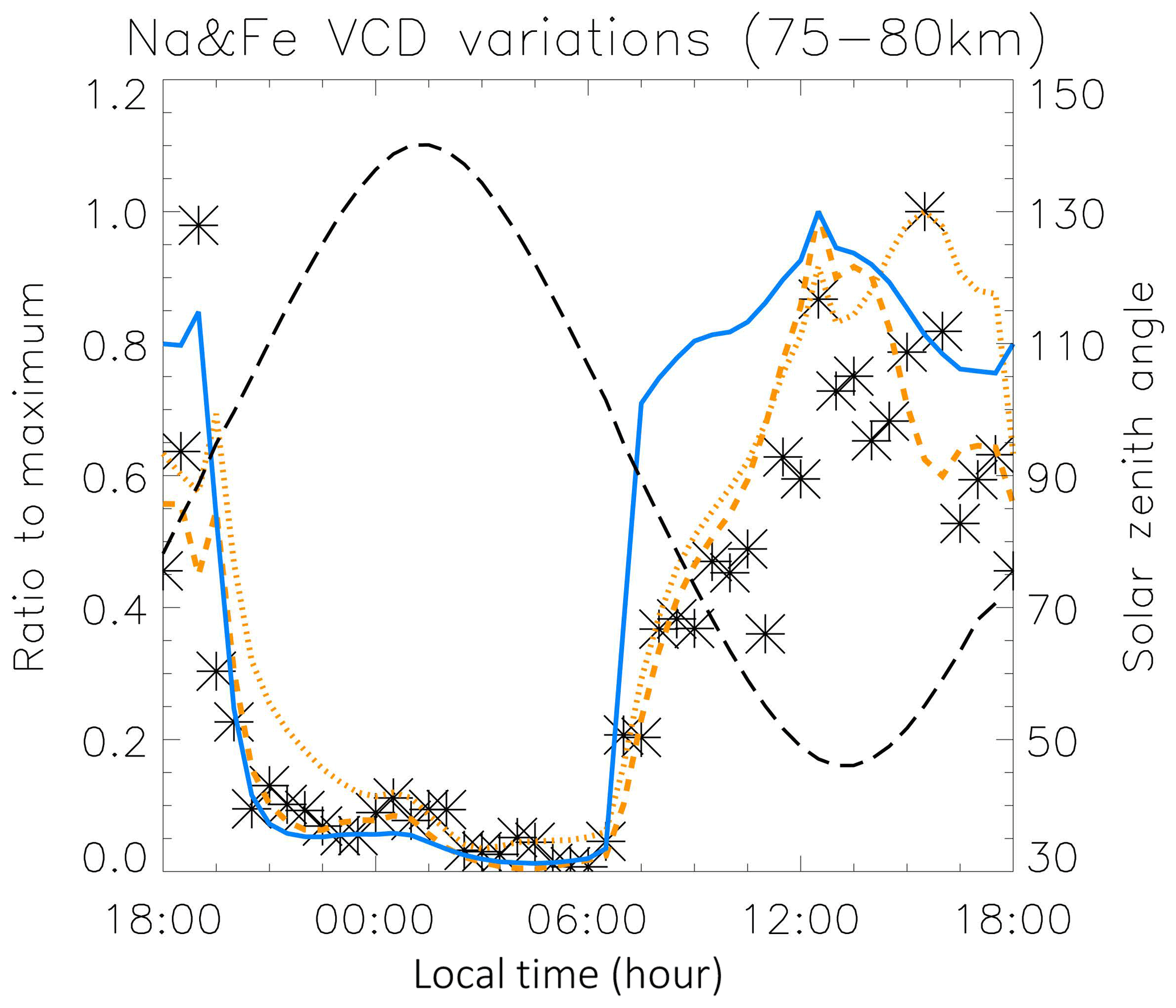
Figure 3The variations in Na VCD (75–80 km) measured the USU Na lidar during the 7-day Na lidar campaign (asterisks), simulated by WACCM_Na 88-level run (orange dotted line) and 144-level run (orange dashed line) and solar zenith angle (black long-dashed line), along with Fe VCD (75–80 km), simulated by the WACCM_Fe 144-level run (blue solid line).
An interesting contrast can be made with the behavior in the bottom side of the mesospheric Fe layer, where considerable density variations due to photolysis have also been observed by Fe lidars within a similar altitude range (Yu et al., 2012; Viehl et al., 2016). Also included in Fig. 3 is the modeled variation in the Fe VCD between 75 and 80 km, using a lev144 simulation with WACCM-Fe, which has been validated against Fe lidar observations (Viehl et al., 2016). Note that, although the rate of decrease in the Fe VCD around sunset is almost identical to that of Na (because both species correlate with the falling O and H concentrations after sunset), the rate of increase at sunrise is significantly faster. The Fe VCD reaches 70 % of its daytime maximum within about 1 h, whereas the Na VCD takes more than 4 h to reach the same percentage of its maximum.
During the solar eclipse on 21 August 2017, the USU Na lidar conducted a special campaign to observe its potential impact on the MLT. The lidar beam was pointed to the north, 30∘ off zenith, and operated between 09:45 and 15:00 LT. Although this campaign was limited by poor sky conditions in the early morning and afternoon, it was able to cover the complete course of the solar eclipse and observe the MLT at the peak of the eclipse with more than 96 % of totality at 11:34 LT. To our knowledge, these are the first lidar observations in the MLT during an eclipse.
The lidar-observed mesospheric Na density variations during the event are shown in Fig. 4, and the temporal resolution is 10 min. The averaged return signal between 200 and 220 km altitude per lidar line-of-sight (LOS) binning range (150 m) is treated as the sky background, which is also shown in Fig. 4. The background variation indicates that at the USU location the eclipse began at 10:25 LT, peaked at 11:34 LT and ended just before 13:00 LT. The high background before 10:00 LT was due to hazy sky conditions in the early morning, similarly to after 15:00 LT when it became cloudy. During the course of this event, the mesospheric Na layer weakened with decreasing peak density. In particular, Na density variation was more evident below 85 km. As Fig. 4 shows, before the eclipse the constant density lines on the bottom side of the layer were moving downwards (i.e. increasing density at each altitude). As the eclipse unfolded, these constant density lines started to move towards higher altitudes (the density decreased at each altitude). During the recovery phase of the eclipse, the Na density began to increase again. By ∼13:00 LT, the Na layer was fully recovered, and no significant change was observed on the bottom side of the layer. For example, the density line of 450 cm−3 was near 80 km right before the eclipse started. It moved upward to near 81.5 km at the culmination of the event, before it went back and stayed near 80 km at the end of the event. Similar behavior can be seen in all constant density lines below 85 km. Further calculation of the lidar measured bottom side Na VCD (75–85 km) shows that it decreased by about 40 % between 10:25 and 11:35 LT.
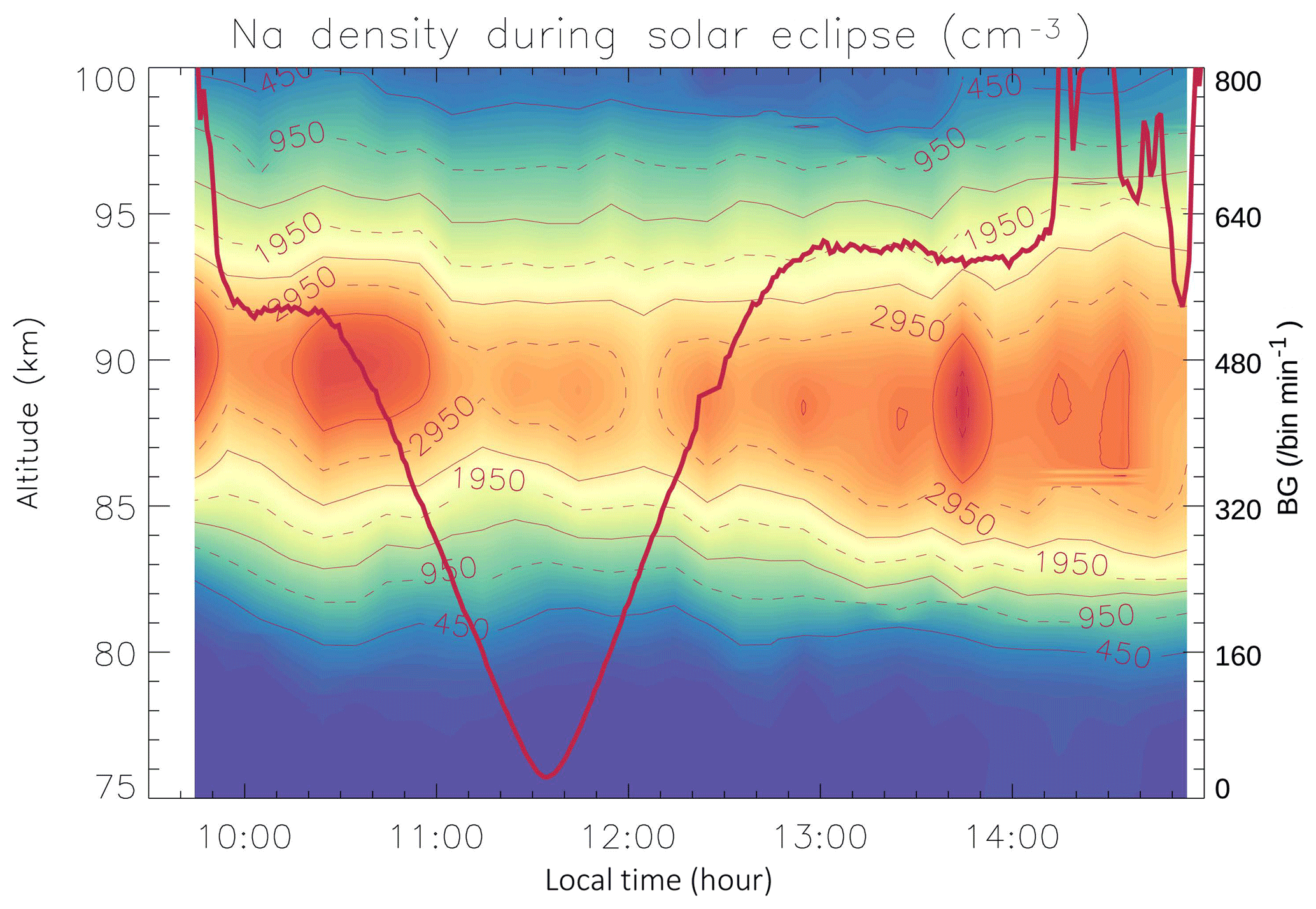
Figure 4The mesospheric Na density variation during the solar eclipse on 21 August 2017, observed by the Na lidar at Utah State University. The red solid line represents the lidar-detected sky background. The unit for the lidar background measurement is bin−1 min−1.
The simultaneous temperature and horizontal wind measurements during the eclipse, however, do not reveal apparent variations that can be associated with the event (not shown). For instance, the measured temperature change is within the daytime lidar measurement uncertainty (∼5 K with 20 min and 4 km smoothing). The temperature change during the solar eclipse is expected to be that small when considering the general energy budget in the MLT. When the short-wave heating that dominates the daytime budget (mainly exothermic heating from atomic O recombination) is turned off (Brasseur and Solomon, 2005), infrared cooling due to CO2 emissions would lead to net cooling in the mesopause region. However, the magnitude of this cooling is only about 1 K h−1 (Roble, 1995). Thus, for a solar eclipse that only lasts for 2 h with just a few minutes of totality, a noticeable temperature change should not occur. This result is consistent with a recent simulation of the eclipse using the WACCM-X model, which concluded that the temperature variation in the mesosphere would have been no more than 4 K (McInerney et al., 2018). Furthermore, the variation in temperature within this range will not have a significant impact on the Na reaction kinetics and hence the Na atom density (Plane et al., 1999).
The major reservoir for Na on the bottom side of the layer is NaHCO3, which forms in three steps from Na atoms: oxidation of Na by O3 to NaO, reaction with H2O or H2 to form NaOH and recombination of NaOH with CO2 (Plane et al., 2015; Gómez-Martín et al., 2017). NaHCO3 is converted back to Na either by photolysis (reaction R4) or by reaction with atom H in (R9). The rate coefficient for this reaction, (R9), is T0.78 exp() cm3 molecule−1 s−1 (Cox et al., 2001), which is cm3 molecule−1 s−1. The typical daytime H concentration between 75 and 80 km is around 5×107 cm−3 (Plane et al., 2015), so the first-order rate of this reaction is s−1, which is about 40 times slower than R4. Thus, photolysis of NaHCO3, which has built up during the night, is responsible for ∼98 % of the increase in the Na VCD after sunrise (Fig. 3). The excellent agreement between the laboratory-measured photolysis rate of NaHCO3 (Self and Plane, 2002), and the observed increase in the Na VCD is strong evidence that NaHCO3 is indeed the major Na reservoir on the bottom side of the Na layer. Indeed, as shown in Fig. 5, the WACCM_Na-simulated variations of Na, H and O, between local midnight and noon, are highly correlated in the upper mesosphere in the same 144-level run. Within the same region, the NaHCO3 density decreases above 78 km after sunrise due to photolysis and the increases in H and O. Below this altitude, the change in NaHCO3 is much smaller because the concentrations of O and H despite increasing after sunrise, are too small to prevent any Na produced being rapidly converted back to NaHCO3. This is because the initial oxidation step – the recombination reaction of Na with O2 (which is a pressure-dependent) – becomes very fast below 78 km.
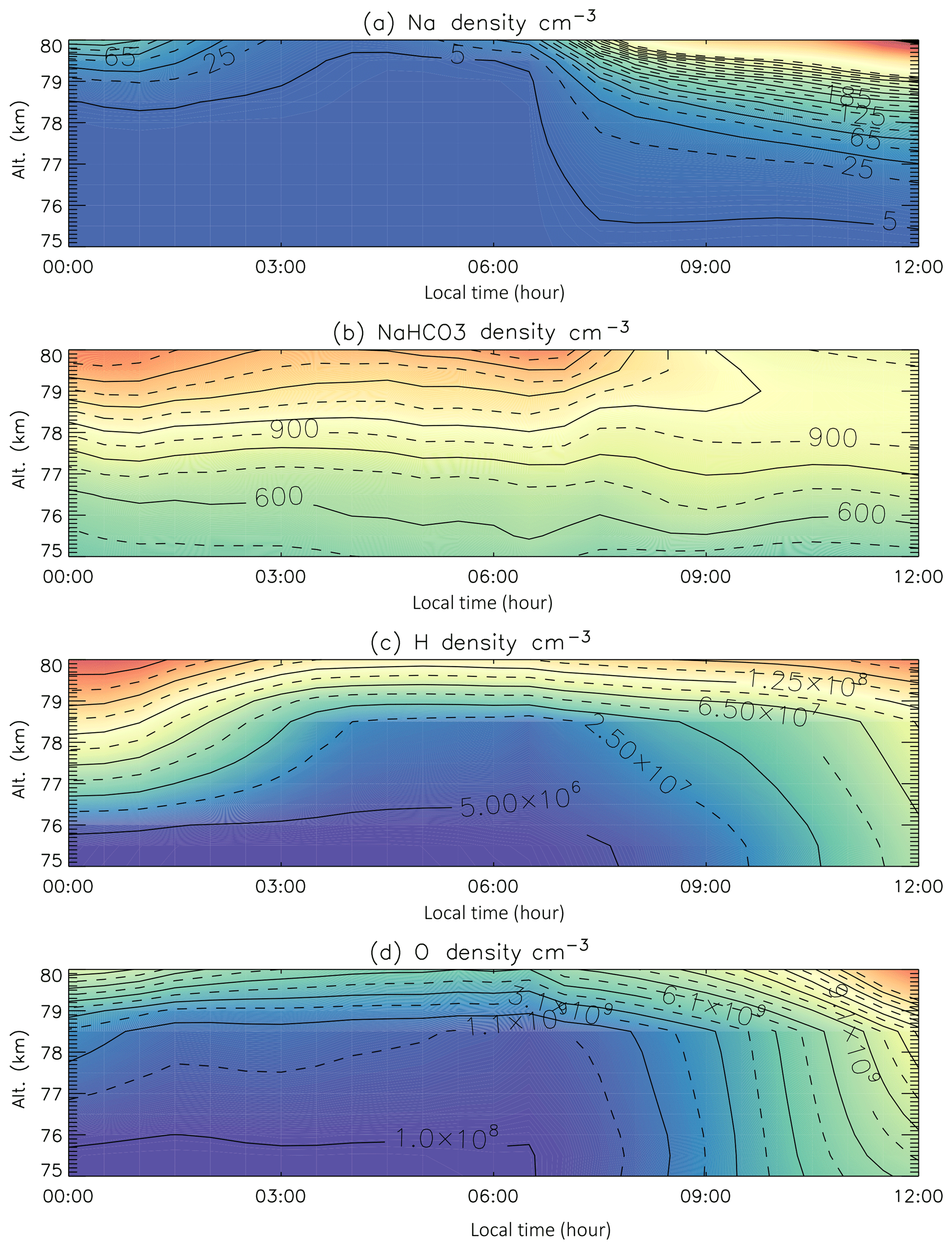
Figure 5The variations of Na (a), NaHCO3 (b), H (c) and O (d) on the bottom side of the mesospheric Na layer, simulated by the WACCM_Na_144-level run.
Based on the above discussion, a decrease in Na on the bottom side of the layer would be expected during the eclipse because of the reduction in the photolysis rates (R1–R4) and atomic O and H. As shown in Fig. 4, a decrease in the Na density below 85 km was indeed observed by the lidar during this period. However, the decrease in Na is relatively small when compared with the natural variability measured with the USU Na lidar during the morning hours (observed over 50 days of lidar data between 20 August and 30 September in 2011–2016), which can be as much as 60 % between 75 and 85 km, and is mostly driven by atmospheric gravity wave modulations (Shelton et al., 1980). The effect of the eclipse was modeled by driving a 1-D model of the Na layer (0.5 km vertical resolution, 5 min time resolution) (Plane, 2004) with the background atmospheric species (O3, O, H etc.) from the WACCM-X simulation of the eclipse (McInerney et al., 2018). As shown in Fig. 6, the modeled decrease in Na around 80 km is within the natural variability and much less than the diurnal change in the bottom side of the layer because the time in which photolysis is significantly reduced during the eclipse is too short.
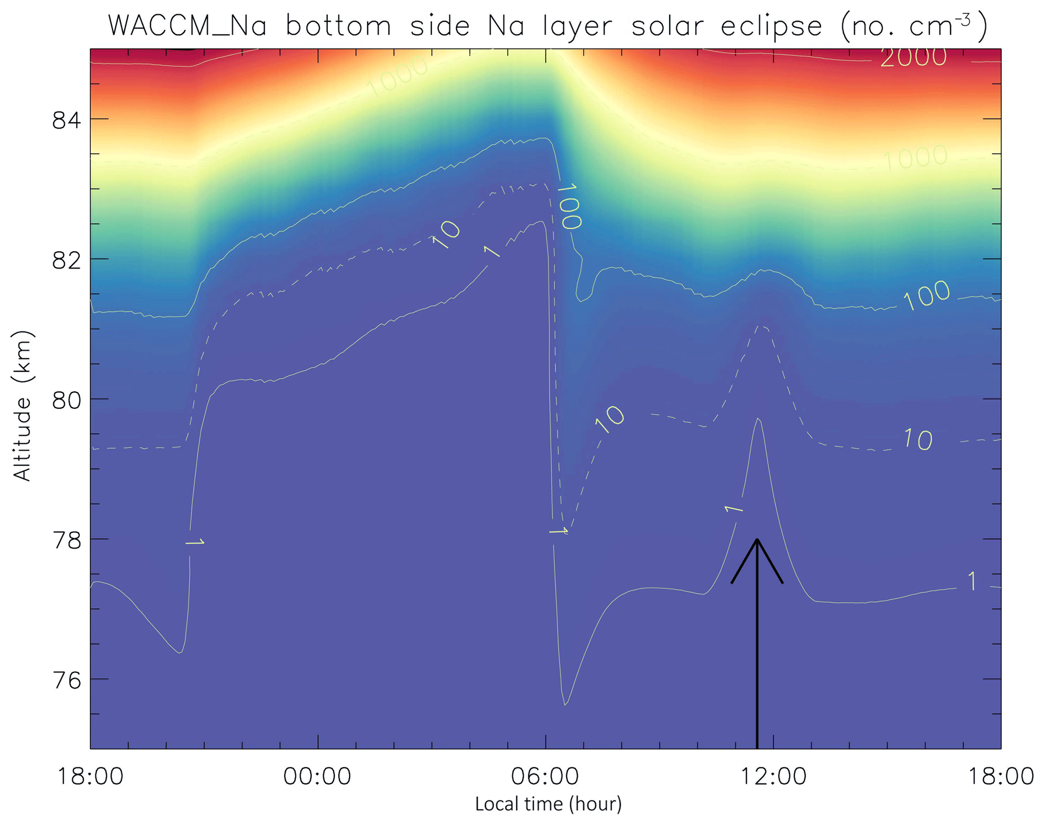
Figure 6A 1-D model simulation of the Na layer variation during the solar eclipse between 18:00 LT on 20 August and 18:00 LT 21 August in 2017. The solar eclipse at the USU Na lidar location peaked at 11:34 on 21 August (marked by the solid arrow). The background atmospheric species (O3, O, H, etc.) are based on the outputs of WACCM-X eclipse simulation.
In terms of the mesospheric Fe layer, the major Fe reservoir in this region is most likely FeOH (Self and Plane, 2003; Plane, 2004; Plane et al., 2015). Similarly to Na, the dominant Fe production processes within the bottom half of the layer involve a reaction with H and photolysis:
The rate coefficients of both these reactions are considerably higher than those of the analogous Na reactions, particularly R11, which is faster than R4 by more than 2 orders of magnitude (Viehl et al., 2016). It is this feature which controls the more rapid appearance of Fe around 80 km after sunrise, as shown in Fig. 4. Note that this rapid increase has been previously observed by lidar (Viehl et al., 2016; Yu et al., 2012).
Observations of the full diurnal cycle of the bottom side of the mesospheric Na layer reveal substantial changes in Na density near and below 80 km, with more than an order-of-magnitude increase after sunrise, while the change in Na density above 90 km during the same process is relatively slow. In this study we show that this diurnal variation is largely driven by the photochemistry of the major reservoir species NaHCO3. This result is established by demonstrating reasonable agreement between USU lidar observations of the Na layer below 80 km and a whole atmosphere chemistry-climate model which includes a comprehensive Na chemistry module (WACCM-Na). Indirect photochemistry, where atomic H and O are produced by the photolysis of O3, O2 and H2O, and these atoms then reduce Na compounds (NaHCO3, NaOH, NaO and NaO2) back to Na, also plays an important role in the diurnal variability. The more rapid increase in atomic Fe after sunrise, which has been observed at several locations (Viehl et al., 2016; Yu et al., 2012), is consistent with the much faster rate of photolysis of FeOH compared with NaHCO3. Lidar observations made during the solar eclipse on 21 August 2017 (at a location with 96 % totality) did not reveal significant changes in either temperature or Na density that were larger than the natural variability around 80 km. This is consistent with a recent study using WACCM-X (McInerney et al., 2018) and the Na model results presented here.
The USU Na lidar data of this study before 2018 are available at the Consortium of Resonance and Rayleigh Lidars (CRRL) Madrigal data base at http://madrigal.physics.colostate.edu/htdocs/ (last access: 30 April 2017). The lidar data from 2018 can be accessed through “USU Na lidar Data” (https://doi.org/10.15142/T33H26, Yuan, 2018).
TY was responsible for the lidar operations and the associated experimental data analysis that are related to this work. WF conducted the numerical simulations using the WACCM-Na and WACCM-Fe. JMCP and DRM provided the chemical and atmospheric dynamic theories for this collaborative work.
The authors declare that they have no conflict of interest.
This article is part of the special issue “Layered phenomena in the mesopause region (ACP/AMT inter-journal SI)”. It is a result of the LPMR workshop 2017 (LPMR-2017), Kühlungsborn, Germany, 18–22 September 2017.
The lidar work in this study was performed as part of a collaborative research programme supported under the CRRL National Science Foundation (NSF) grant AGS1135882, with additional support from NSF grants AGS1734333, and N000141712149 of Naval Research Laboratory. The National Center for Atmospheric Research is sponsored by the NSF. John M. C. Plane and Wuhu Feng acknowledge funding from the European Research Council (project number 291332-CODITA).
This paper was edited by William Ward and reviewed by two anonymous referees.
Brasseur, G. P. and Solomon, S.: Aeronomy of the Middle Atmosphere: Chemistry and Physics of the Stratosphere and Mesosphere, Springer, New York, 2005.
Carrillo-Sánchez, J. D., Nesvorný, D., Pokorný, P., Janches, D., and Plane, J. M. C.: Sources of cosmic dust in the Earth's atmosphere, Geophys. Res. Lett., 43, 11979–11986, https://doi.org/10.1002/2016GL071697, 2016.
Chen, H., White, M. A., Krueger, D. A., and She, C. Y.: Daytime mesopause temperature measurements using a sodium-vapor dispersive Faraday filter in lidar receiver, Opt. Lett., 21, 1003–1005, 1996.
Clemesha, D. M., Batista, P. P., and Simonich, D. M.: Tide-induced oscillations in the atmospheric sodium layer, J. Atmos. Sol.-Terr. Phys., 64, 1321–1325, 2002.
Cox, R. M., Self, D. E., and Plane, J. M. C.: A study of the reaction between NaHCO3 and H: apparent closure on the neutral chemistry of sodium in the upper mesosphere, J. Geophys. Res., 106, 1733–1739, 2001.
Dawkins, E. C. M., Plane, J. M. C., Chipperfield, M. P., Feng, W., Marsh, D. R., Höffner, J., and Janches, D.: Solar cycle response and longterm trends in the mesospheric metal layers, J. Geophys. Res.-Space Phys., 121, 7153–7165, https://doi.org/10.1002/2016JA022522, 2016.
Dunker, T., Hoppe, U.-P., Feng, W., Plane, J. M. C., and Marsh, D. R.: Mesospheric temperatures and sodium properties measured with the ALOMAR Na lidar compared with WACCM, J. Atmos. Sol.-Terr. Phys., 127, 111–119, 2015.
Fan, Z. Y., Plane, J. M. C., Gumbel, J., Stegman, J., and Llewellyn, E. J.: Satellite measurements of the global mesospheric sodium layer, Atmos. Chem. Phys., 7, 4107–4115, https://doi.org/10.5194/acp-7-4107-2007, 2007.
Feng, W., Marsh, D. R., Chipperfield, M. P., Janches, D., Hoeffner, J., Yi, F., and Plane, J. M. C.: A global atmospheric model of meteoric iron, J. Geophys. Res.-Atmos., 118, 9456–9474, 2013.
Feng, W., Kaifler, B., Marsh, D. R., Höffner, J., Hoppe, U.-P., Williams, B. P., and Plane, J. M. C.: Impacts of a sudden stratospheric warming on the mesospheric metal layers, J. Atmos. Sol.-Terr. Phys., 162, 162–171, https://doi.org/10.1016/j.jastp.2017.02.004, 2017.
Gómez Martín, J. C., Garraway, S., and Plane, J. M. C.: Reaction Kinetics of Meteoric Sodium Reservoirs in the Upper Atmosphere, J. Phys. Chem. A, 120, 1330–1346, https://doi.org/10.1021/acs.jpca.5b00622, 2016.
Gómez Martín, J. C., Seaton, C., de Miranda, M. P., and Plane, J. M. C.: The Reaction between Sodium Hydroxide and Atomic Hydrogen in Atmospheric and Flame Chemistry, The J. Phys. Chem. A, 121, 7667–7674, https://doi.org/10.1021/acs.jpca.7b07808, 2017.
Harrell, S. D., She, C. Y., Yuan, T., Krueger, D. A., Chen, H., Chen, S., and Hu, Z. L.: Sodium and potassium vapor Faraday filters re-visited: Theory and applications, J. Opt. Soc. Am. B, 26, 659–670, 2009.
Hurrell, J. W., Hack, J. J., Phillips, A. S., Caron, J., and Yin, J.: The dynamical simulation of the Community Atmosphere Model version 3 (CAM3), J. Climate, 19, 2162–2183, 2006.
Kinnison, D. E., Brasseur, G. P., Walters, S., Garcia, R. R., Marsh, D. R., Sassi, F., Harvey, V. L., Randall, C. E., Emmons, L., Lamarque, J. F., Hess, P., Orlando, J. J., Tie, X. X., Randel, W., Pan, L. L., Gettelman, A., Granier, C., Diehl, T., Niemeier, U., and Simmons, A. J.: Sensitivity of chemical tracers to meteorological parameters in the MOZART-3 chemical transport model, J. Geophys. Res., 112, D20302, https://doi.org/10.1029/2006JD007879, 2007.
Krueger, D. A., She, C.-Y., and Yuan, T.: Retrieving mesopause temperature and line-of-sight wind from full-diurnal-cycle Na lidar observations, Appl. Opt., 54, 9469–9489, 2015.
Lamarque, J.-F., Emmons, L. K., Hess, P. G., Kinnison, D. E., Tilmes, S., Vitt, F., Heald, C. L., Holland, E. A., Lauritzen, P. H., Neu, J., Orlando, J. J., Rasch, P. J., and Tyndall, G. K.: CAM-chem: description and evaluation of interactive atmospheric chemistry in the Community Earth System Model, Geosci. Model Dev., 5, 369–411, https://doi.org/10.5194/gmd-5-369-2012, 2012.
Langowski, M. P., von Savigny, C., Burrows, J. P., Fussen, D., Dawkins, E. C. M., Feng, W., Plane, J. M. C., and Marsh, D. R.: Comparison of global datasets of sodium densities in the mesosphere and lower thermosphere from GOMOS, SCIAMACHY and OSIRIS measurements and WACCM model simulations from 2008 to 2012, Atmos. Meas. Tech., 10, 2989–3006, https://doi.org/10.5194/amt-10-2989-2017, 2017.
Li, T., Ban, C., Fang, X., Li, J., Wu, Z., Feng, W., Plane, J. M. C., Xiong, J., Marsh, D. R., Mills, M. J., and Dou, X.: Climatology of mesopause region nocturnal temperature, zonal wind and sodium density observed by sodium lidar over Hefei, China (32∘ N, 117∘ E), Atmos. Chem. Phys., 18, 11683–11695, https://doi.org/10.5194/acp-18-11683-2018, 2018.
Lin, S.-J.: A “vertically-Lagrangian” finite-volume dynamical core for global atmospheric models, Mon. Weather Rev., 132, 2293–2307, 2004.
Marsh, D. R., Janches, D., Feng, W., and Plane, J. M. C.: A global model of meteoric sodium, J. Geophys. Res.-Atmos., 118, 11442–11452, https://doi.org/10.1002/jgrd.50870, 2013.
McInerney, J. M., Marsh, D. R., Liu, H.-L., Solomon, S. C., Conley, A. J., and Drob, D. P.: Simulation of the 21 August 2017 solar eclipse using the Whole Atmosphere Community Climate Model-eXtended, Geophys. Res. Lett., 45, 3793–3800, https://doi.org/10.1029/2018GL077723, 2018.
Merkel, A. W., Marsh, D. R., Gettelman, A., and Jensen, E. J.: On the relationship of polar mesospheric cloud ice water content, particle radius and mesospheric temperature and its use in multi-dimensional models, Atmos. Chem. Phys., 9, 8889–8901, https://doi.org/10.5194/acp-9-8889-2009, 2009.
Neale, R. B., Richter, J., Park, S., Lauritzen, P., Vavrus, S., Rasch, P., and Zhang, M.: The mean climate of the Community Atmosphere Model (CAM4) in forced SST and fully coupled experiments, J. Climate, 26, 5150–5168, https://doi.org/10.1175/JCLI-D-12-00236.1, 2013.
Plane, J. M. C.: Atmospheric chemistry of meteoric metals, Chem. Rev., 103, 4963–4984, https://doi.org/10.1021/cr0205309, 2003.
Plane, J. M. C.: A time-resolved model of the mesospheric Na layer: constraints on the meteor input function, Atmos. Chem. Phys., 4, 627–638, https://doi.org/10.5194/acp-4-627-2004, 2004.
Plane, J. M. C., Gardner, C. S., Yu, J., She, C. Y., Garcia, R. R., and Pumphrey, H. C.: Mesospheric Na layer at 40N: Modeling and observations, J. Geophys. Res., 104, 3773–3788, 1999.
Plane, J. M. C., Saunders, R. W., Hedin, J., Stegman, J., Khaplanov, M., Gumbel, J., Lynch, K. A., Bracikowski, P. J., Gelinas, L. J., Friedrich, M., Blindheim, S., Gausa, M., and Williams, B. P.: A combined rocket-borne and ground-based study of the sodium layer and charged dust in the upper mesosphere, J. Atmos. Sol.-Terr. Phys., 118, 151–160, 2014.
Plane, J. M. C., Feng, W., and Dawkins, E. C. M.: The mesosphere and metals: Chemistry and changes, Chem. Rev., 115, 4497–4541, https://doi.org/10.1021/cr500501m, 2015.
Plane, J. M. C., Feng, W., Gómez Martín, J. C., Gerding, M., and Raizada, S.: A new model of meteoric calcium in the mesosphere and lower thermosphere, Atmos. Chem. Phys., 18, 14799–14811, https://doi.org/10.5194/acp-18-14799-2018, 2018.
Roble, R. G.: Energetics of the mesosphere and thermosphere, in: The Upper Atmosphere and Lower Thermosphere: A Review of Experiment and Theory, edited by: Johnson, R. M. and Killeen, T. L., American Geophysical Union, Washington, DC, 1995.
Sandford, M. C. W. and Gibson, A. J.: Laser radar measurements of the atmospheric sodium layer, J. Atmos. Terr. Phys., 32, 1423–1430, 1970.
Self, D. E. and Plane, J. M. C.: Absolute photolysis cross-sections for NaHCO3 , NaOH, NaO, NaO2 and NaO3: implications for sodium chemistry in the upper mesosphere, Phys. Chem. Chem. Phys., 4, 16–23, https://doi.org/10.1039/B107078A, 2002.
Self, D. E. and Plane, J. M. C.: A kinetic study of the reactions of iron oxides and hydroxides relevant to the chemistry of iron in the upper mesosphere, Phys. Chem. Chem. Phys., 5, 1407–1418, https://doi.org/10.1039/b211900e, 2003.
Shelton, J. D., Gardner, C. S., and Sechrist Jr., C. F.: Density response of the mesospheric sodium layer to gravity wave perturbations, Geophys. Res. Lett., 7, 1069–1072, 1980.
States, R. J. and Gardner, C. S.: Structure of mesospheric Na layer at 40N latitude: seasonal and diurnal variations, J. Geophys. Res., 104, 11783–11798, 1999.
Viehl, T. P., Plane, J. M. C., Feng, W., and Höffner, J.: The photolysis of FeOH and its effect on the bottomside of the mesospheric Fe layer, Geophys. Res. Lett., 43, 1373–1381, https://doi.org/10.1002/2015GL067241, 2016.
Yu, Z., Chu, X., Huang, W., Fong, W., and Roberts, B. R.: Diurnal variations of the Fe layer in the mesosphere and lower thermosphere: Four season variability and solar effects on the layer bottomside at McMurdo (77.8∘ S, 166.7∘ E), Antarctica, J. Geophys. Res., 117, D22303, https://doi.org/10.1029/2012JD018079, 2012.
Yuan, T., She, C.-Y., Kawahara, T. D., and Krueger, D. A.: Seasonal variations of mid-latitude mesospheric Na layer and its tidal period perturbations based on full-diurnal-cycle Na lidar observations of 2002–2008, J. Geophys. Res., 117, D1130, https://doi.org/10.1029/2011JD017031, 2012.
Yuan, T., She, C. Y., Oberheide, J., and Krueger, D. A.: Vertical tidal wind climatology from full-diurnal-cycle temperature and Na density lidar observations at Ft. Collins, CO (41∘ N, 105∘ W). J. Geophys. Res.-Atmos., 119, 4600–4615, https://doi.org/10.1002/2013JD020338, 2014.
Yuan, T.: USU Na lidar data, Browse all Datasets, NSF, Division of Atmospheric and Geospace Sciences, Utah State University, https://doi.org/10.15142/T33H26, 2018.