the Creative Commons Attribution 4.0 License.
the Creative Commons Attribution 4.0 License.
 | 22 Mar 2019
Long-term trends of instability and associated parameters over the Indian region obtained using a radiosonde network
Rohit Chakraborty
Madineni Venkat Ratnam
Shaik Ghouse Basha
Long-term trends of the parameters related to convection and instability obtained from 27 radiosonde stations across six subdivisions over the Indian region during the period 1980–2016 are presented. A total of 16 parcel and instability parameters along with moisture content, wind shear, and thunderstorm and rainfall frequencies have been utilized for this purpose. Robust fit regression analysis is employed on the regional average time series to calculate the long-term trends on both a seasonal and a yearly basis. The level of free convection (LFC) and the equilibrium level (EL) height are found to ascend significantly in all Indian subdivisions. Consequently, the coastal regions (particularly the western coast) experience increases in severe thunderstorms (TSS) and severe rainfall (SRF) frequency in the pre-monsoon period, while the inland regions (especially Central India) experience an increase in ordinary thunderstorms (TSO) and weak rainfall (WRF) frequency during the monsoon and post-monsoon periods. The 16–20-year periodicity is found to dominate the long-term trends significantly compared to other periodicities and the increase in TSS, and convective available potential energy (CAPE) is found to be more severe after the year 1999. The enhancement in moisture transport and associated cooling at 100 hPa along with the dispersion of boundary layer pollutants are found to be the main causes for the increase in CAPE, which leads to more convective severity in the coastal regions. However, in inland regions, moisture-laden winds are absent and the presence of strong capping effect of pollutants on instability in the lower troposphere has resulted in more convective inhibition energy (CINE). Hence, TSO and occurrences of WRF have increased particularly in these regions.
- Article
(4112 KB) -
Supplement
(1201 KB) - BibTeX
- EndNote


Intense convective phenomena are a common climatic feature in the Indian tropical region which occur during the pre-monsoon to post-monsoon seasons (April–October) (Ananthakrishnan, 1977) and are generally accompanied by intense thunderstorms, lightning, and wind gusts with heavy rainfall. Hence, they are known to induce immense socioeconomic hazards including loss of life and property. Several reports have shown an increase in the climatic extreme occurrence and intensity of these phenomena throughout the world (Webster et al., 2005; Emanuel, 2006). In this connection, traditional surface-based parcel theory has been utilized to understand convective processes using atmospheric soundings as it calculates the atmospheric instabilities and other parameters at various heights (Huntrieser et al., 1997; Santhi et al., 2014; Narendra Reddy et al., 2018).
Considering the importance of studying the long-term trends in climatic extremes, a series of research attempts have been orchestrated to study and predict intense convection worldwide in the last two decades (Das et al., 2017). Using multiple tropical stations and reanalysis data, Gettleman et al. (2002) and Riemann-Campe et al. (2009) have shown that convective available potential energy (CAPE) increased very strongly with a growth rate of ∼20 % per decade during the period 1958–1997 due to an increase in surface heating and moisture. Gensini and Mote (2015) projected a 236 % increase in severe thunderstorm frequency from 1980–1990 to 2080–2090 over the eastern United States (US). Further, Brooks (2013) used various combinations of CAPE and vertical wind shear products, and results hinted towards a probable increase in severe thunderstorms over the US. It was also observed that the effect of increasing CAPE is more dominant on convective severity than in the case of decreasing shear. On the other hand, studies by Prein et al. (2017) showed that a recent increase of temperature has led to a rise of moisture ingress, and consequently the frequency and severity of extreme precipitation events associated with intense convection have shown a steep rise everywhere in the world. At the same time, an increase in thunderstorm severity and instability has also been reported by many studies over the Asian region (Wang et al., 2011; Saha et al., 2017).
Over the Indian region, Manohar et al. (1999) studied the latitudinal variation and distribution of thunderstorm frequency and CAPE over 78 Indian stations during 1970–1980 and they postulated that the ambient temperature at the 100 hPa pressure level has a strong relationship with it. Dhaka et al. (2010) utilized radiosonde observations during 1958–1997 and they obtained very prominent anti-correlations on both a yearly and a seasonal basis between convection strength (CAPE) and upper-troposphere temperatures at 100 hPa (T100). Later, Murugavel et al. (2012) studied the long-term trends of CAPE from 32 radiosonde stations during 1984–2008 and revealed an alarming growth in monsoon CAPE over India, with a slope of 38 J kg−1 year−1. However, they additionally stated that the low-level moisture and solar cycle can have an additional impact on the increasing CAPE. Recently, Chakraborty et al. (2017a) and Saha et al. (2017) reported a weakening in lower tropospheric instability over a few Indian stations due to increasing pollution levels using reanalysis datasets. Apart from that, some studies have also attempted to correlate convective severity with boundary layer phenomena, upper-tropospheric moisture, surface fluxes, the solar effect, and precipitation (Basha and Ratnam, 2013; Basha et al., 2013; Murthy and Sivaramakrishnan, 2006; Allappattu and Kunnikrishnan, 2009; Xie et al., 2011; Nelli et al., 2018; Rakshit et al., 2016).
Previous studies over India have shown the distribution of CAPE only, whereas other parameters like convective inhibition energy (CINE), mixed layer CAPE (MLC), lifted index (LI), Total Totals Index (TTI), and precipitable water vapor (PWV) are also important as they explain how the atmospheric instability and moisture change at various levels of the atmosphere. In addition, the influence of climatic oscillation (Quasi-Biennial Oscillation, QBO, El Niño–Southern Oscillation, ENSO, and the solar cycle) on the seasonal and annual variation of convective parameters was also not studied in detail. Therefore in the present study, the long-term variation of parcel parameters (lifted condensation level, LCL, level of free convection, LFC, equilibrium level, EL, CAPE, and CINE), with instability (LI, Vertical Totals Index, VT), moisture (PWV, and PWV at low levels, PWL), thunderstorm and rainfall severity frequencies (severe thunderstorms, TSS, ordinary thunderstorms, TSO, weak rainfall, WRF, and strong rainfall, SRF), followed by temperature at 100 hPa (T100) and wind shear (WSH), is investigated using 27 radiosonde stations along with gridded rainfall data over India. This article is structured as follows: Sect. 2 describes the datasets and methodology adopted for the present study. Section 3 presents the long-term analysis of parcel and instability parameters over Chennai (13.08∘ N, 80.27∘ E) and six subdivisions of the Indian subcontinent on both an annual and a seasonal basis, followed by the periodicity and split trend analysis. Finally, a discussion on the results and conclusions are given in Sects. 4 and 5, respectively.
Radiosonde observations from 27 stations over the Indian region from 1980 to 2016 are obtained from the Integrated Global Radiosonde Archive (IGRA; https://www1.ncdc.noaa.gov/pub/data/igra/derived/derived-por/, IGRA2, 2019). These datasets provide daily temperature and humidity profiles from 1538 stations around the world at fixed pressure levels after quality checks have been done (Durre et al., 2006; Ferreira et al., 2018). These studies have concluded that the radiosonde data quality from IGRA has faced certain problems from time to time, but such cases are not so prominent over the Indian region, especially after the year 1980. It is mainly because of the higher accuracy and reliability of this in situ measurement technique that these datasets are widely used worldwide nowadays for calibrating other continuous profiler instruments (Chakraborty and Maitra, 2016). In accordance with data availability and reliability, only 27 stations have been considered out of 37 IGRA Indian radiosonde stations, thereby providing decent data availability for carrying out this study. When an in-depth investigation is done on the data continuity by plotting the temperature and humidity profiles for all days, a set of gaps in datasets was discovered. Most of the utilized stations have intermittent data gaps of 2–7 days in certain months only, but, on the whole, except only a very few cases, the duration of these individual data gaps is mostly limited to less than 1 month. However, these small data gaps are not expected to provide any significant impact on the long-term seasonal or annual average variations with a span of 37 years.
In addition to data availability, homogeneity is also a common concern before data are used. However, such issues should not be considered to be serious as all three types of homogeneity issues, namely volume, instrument type, and quality, were addressed before the study was commenced. First, about 5000 radiosonde profiles are available at the majority of IGRA stations which are uniformly distributed among all years and seasons (except the monsoon); hence it provides a decent data volume for the investigation of yearly trends. Secondly, the data of all Indian IGRA stations come from a single type of IM-MK3 radiosondes, which has not undergone any change in radiosonde accuracies in recent years; so this addresses the instrument-type-related issue. Finally, regarding data quality, a set of seven quality checks are performed by IGRA before the data are accepted, which should remove any unreliable observations before they are used in the study. These seven quality checks also include a repetition check, which rejects any possible case of humidity sensor saturation errors during rainy conditions, especially in the monsoon. Thus it can be inferred that the obtained climatic trends of instability from IGRA are expected to be far more reliable compared to other data sources.
These 27 stations have been divided into six homogenous regions as defined by the India Meteorological Department (IMD) (Rao, 1976), which are Central India (CI), East Coast (EC), North East (NE), North West (NW), Peninsular India (PI), and the West Coast (WC), as shown in Fig. 1. Further, for simplicity, these regions have again been combined into three major categories, namely coastal regions (EC and WC), inland regions (CI and PI), and others (NE and NW). After retrieving the profiles, some more additional internal quality checks are performed before the data from every IGRA station are used. First, the balloon burst height has to be a minimum of 15 km to be selected for analysis. Second, any gaps of temperature and humidity in important pressure levels such as 850, 700, 500, 300, 200, and 100 hPa will produce difficulty in the calculation of atmospheric instability; hence those profiles were rejected in quality control tests for all stations. Again, out of the available radiosonde profiles, some profiles have displayed very strong variations of temperature and humidity at various heights, and hence they are discarded. After completion of these quality checks, it was thought that atmospheric instability shows prominent diurnal variation, so datasets of only one time slot could be taken for analysis. As datasets at 00:00 Z are more in number than at 12:00 Z, the analysis was actually completed with 00:00 Z datasets. Further details about the final dataset used for every station are given in Table A1. It may be noted here that the volume of observations is found to be distributed almost homogenously throughout the measurement period, and a detailed year-wise breakdown of radiosonde launches utilized is not shown in order to maintain the focus of the work. For calculation of the instability parameters, the temperature and humidity profiles were transformed from the standard pressure levels using cubic spline interpolation for every 100 m height bin. Piece-wise linear, quadratic, and cubic spline interpolation schemes are employed instead of linear interpolation in temperature and humidity retrievals in this study as the former techniques can more reliably regenerate the nonlinearities in boundary layer variations of meteorological parameters according to recent studies by Chakraborty et al. (2016). After this, a similar surface-based parcel method is utilized for estimating the parcel and instability parameters (LCL, LFC, EL, CAPE, MLC, CINE) as already described by Chakraborty et al. (2018). More detail about the physical significance of these parameters is given in the Supplement. For thunderstorm genesis, moisture growth and wind shear are extremely important; therefore we calculated the total amount of water vapor (PWV) and that up to the 700 hPa level (PWL), along with the horizontal wind shear between the surface and 6 km altitude. In addition to these factors, we have used temperature at the 100 hPa pressure level as it is found to strongly influence the convective strengths over the Indian region (Manohar et al., 1999; Dhaka et al., 2010).

Figure 1The locations of the 27 IGRA stations used for the present study. The distribution of the 27 stations over Indian regions is as follows: 4 stations in CI, 6 stations in EC, 4 stations in NE, 4 stations in NW, 5 stations in PI, and finally 4 stations in WC.
Along with these parameters, the long-term impact of instability on convection has also been studied from thunderstorm and rain frequencies. Daily measurements of surface wind speeds are obtained for all the radiosonde observations at 00:00 Z using the University of Wyoming website (http://weather.uwyo.edu/upperair/sounding.html, last access: 18 March 2019). The thunderstorm frequencies are calculated on a yearly basis, based on the criterion given by IMD (http://imd.gov.in/section/nhac/termglossary.pdf, last access: 10 May 2018). According to this criterion, if the maximum surface wind speed is greater than 62 km h−1, then it is considered to be a severe thunderstorm event; otherwise, if wind speeds are between 31 and 62 km h−1, then it is considered to be an ordinary thunderstorm case (also used by Saha et al., 2014). Hereafter, the total number of thunderstorm occurrences per year in both the severe and ordinary category is counted and represented by TSS and TSO. Here it may be noted that the wind speed measurements are taken from the first measurement of the radiosonde balloon flight for all stations. These datasets are always within 10 m of the surface, and according to the WMO criterion, they can assume a maximum error of 1 m s−1 from the surface to the 100 hPa level. Since a minimum wind speed of 31 km h−1 or 8.61 m s−1 is required for identification as an ordinary thunderstorm, this 1 m s−1 error is not expected to perturb the thunderstorm severity climatology presented in this study. In the same way, IMD has provided daily rainfall accumulations in 0.25∘ spatial resolution over the Indian region since the year 1900 (Rajeevan et al., 2006, 2008; Pai et al., 2014). These daily precipitation data at the closest grid point are used to define the frequency of severe and weak rainfall days, hereafter referred to as WRF and SRF, respectively. The severe rainfall frequencies constitute those days on which the daily accumulation is greater than 124.5 mm day−1, while for the weak rainfall cases, it is less than 7.5 mm day−1 according to the IMD glossary as given at http://imd.gov.in/section/nhac/termglossary.pdf (last access: 10 May 2018).
From the previous section it follows that a set of 14 parcel parameters with rainfall and thunderstorm frequencies is essential to understand the convective climatology over India. However, other than this, eight standard instability parameters (LI, KI, TTI, CT, VT, CAPE, CINE, and MLC) are also additionally important to quantify the thunderstorm severity; hence they must also be considered for analysis. Now, it is known that most of these instability parameters are interrelated; hence principal component analysis (PCA) is done to identify and use only those instability parameters that can give a complete but independent overview of the atmospheric instability using minimum parameters. In this analysis, introduced by Hotelling (1936), a set of possibly related parameters is converted into orthogonal independent components after which the primary components are plotted with the initial parameters. Parameter variance scores present at the farthest distance from the primary principal components and also from all the other variables contain the highest variance; hence they are selected for representing the existing group of old inputs. Hence in the present study, daily datasets of all six instability parameters are averaged to yearly values for every regions, and then the PCA is performed on the datasets. Daily datasets have not been directly used for PCA as they would have too many fluctuations which would make the redundant parameter identification very difficult in all cases. The variance distribution plot (not shown) for each region showed that only the first two components contribute to more than 70 % of the total variance; hence the covariance scores of these two strongest orthogonal components are plotted in Fig. 2, which depicts the fact that the LI is completely unrelated to the rest of the parameters. Again, since VT is found to lie exactly in the middle of the rest of the parameters, and it also represents the lower tropospheric instability in a much more suitable way, this parameter is also used with LI to represent the rest of the instability parameters in a convenient way. Consequently, LI and VT are additionally considered along with the previous set of 14 attributes to get the final set of 16 parameters for further analysis.
Table 1Statistical information related to the 37-year trend of all instability parameters over the six subdivisions of India (μ: long-term average, σ: standard deviation, %: total percentage trend).
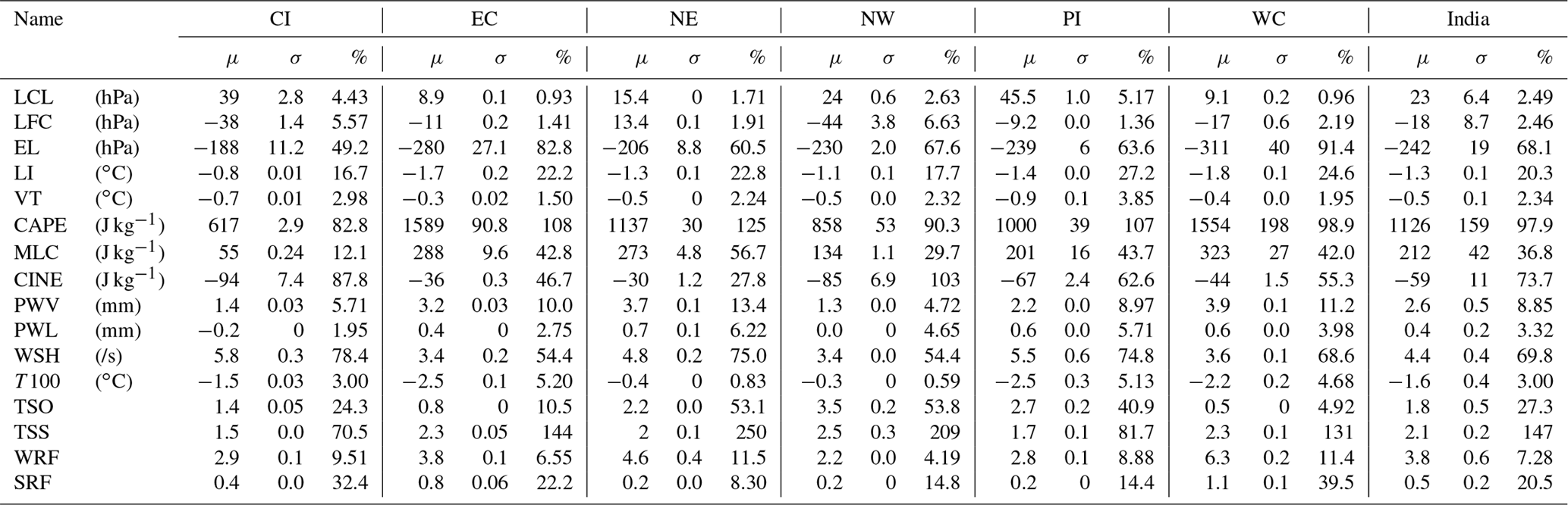

Figure 2Principle component analysis (PCA) for the selection of instability parameters for the long-term trend study in (a) Central India (CI), (b) East Coast (EC), (c), North East (NE), (d) North West (NW), (e) Peninsular India (PI), and (f) West Coast (WC) obtained using IGRA observations.
Thus, a set of 16 parameters is finally taken for the analysis: LCL, LFC, EL, LI, VT, CAPE, CINE, MLC, PWV, PWL, WSH, T100, TSO, TSS, WRF, and SRF. However, apart from the IGRA radiosonde and the IMD rainfall database, it was believed that some other parameters may also be externally responsible for the changing trends in atmospheric instability, and hence they are also included. They comprise the monthly mean Aerosol Absorption Index (AAI) data taken from the Tropospheric Emission Monitoring Internet Service (TEMIS) air pollution archive (De Graaf et al., 2005). In addition, the monthly average gridded data of ozone mixing ratio and specific humidity along with downward longwave radiation flux (DLWRF) are also utilized from ERA-Interim Reanalysis datasets (https://apps.ecmwf.int/datasets/data/interim-full-daily/levtype=sfc/, last access: 6 March 2019).
We have estimated all parameters from daily radiosonde data, averaged over seasons and annually to obtain a trend at a 95 % confidence interval using robust regression analysis (Shepard, 1968). Further, the parameters from radiosonde were averaged region-wise, and then the robust fit algorithm is employed on the normalized time series to get the long-term trends (Andersen, 2008; Raj et al., 2018). These yearly trend values are multiplied by 37 to get the total climatological trend in one parameter over the complete data span of 1980–2016. For seasonal trend analysis, the same approach has been utilized for different seasons. The seasonal distribution has been adopted from IMD reports which are as follows: pre-monsoon (March–May), monsoon (June–September), post-monsoon (October–November), and winter (December–February). Further, for studying the periodicities associated with each of these time series, an Empirical Mode Decomposition (EMD) technique is used (Wu and Huang, 2009). Finally, the robust fit analysis is done on each of these components to compare the trends from each periodicity to determine which of the periodicities dominates in each parameter.

Figure 3Long-term variation of (a) LCL, (b) LFC, (c) EL, (d) LI, (e) VT, (f) CAPE, (g) MLC, (h) CINE, (i) PWV, (j) PWL, (k) WSH, (l) T100, (m) TSO, (n) TSS, (o) WRF, and (p) SRF observed over Chennai.
3.1 Climatic trends over Chennai
In the previous study by Chakraborty et al. (2018), long-term trends of instability were investigated over Gadanki (13.5∘N,79.2∘E) situated on a hilly terrain with an altitude of 370 m a.s.l. at a distance of ∼150 km from the eastern coast and the Bay of Bengal. To see whether the observed trends of these parameters behave similarly in the case of IGRA profiles, the climatic trends of instability are also now described over Chennai (13.08∘ N, 80.27∘ E), which is the closest radiosonde station to Gadanki. The yearly averaged datasets are normalized with respect to their climatic mean and are plotted along with 1σ standard errors in Fig. 3, after which robust fit regression analysis (Andersen, 2008) is utilized to obtain the climatological trends in these parameters, as shown by red solid lines in the plots. A decreasing trend in VT and an increase of magnitude in CINE with LI is noticed, which indicates a reduction in the lower atmospheric instability (Fig. 3d, e, h, i). However, CAPE (Fig. 3f) shows significant increasing trends throughout the period. LFC has a slightly ascending trend (∼18 hPa), which leads to increasing CINE and decreasing VT over Chennai, while the EL is found to ascend drastically (Fig. 3c), resulting in an increase in the total instability and CAPE. The increase in height of EL can be caused by a reduction in temperatures in the upper-tropospheric heights (Manohar et al., 1999). Hence, it can be inferred that the reduction in temperatures near 100 hPa (Fig. 3l) plays an important role in modulating the total atmospheric instability and CAPE.
The enhancement in CINE magnitude and reduction in VT leads to the reduction in the frequency of weaker convective systems with medium or lower CAPE values. Again, as CAPE is one of most important parameters that modulate convective severity, the frequency of severe thunderstorms and heavy rainfall occurrences is expected to rise (Fig. 3n, p). Thus, it is inferred that lower-level instability has reduced due to elevated CINE and LFC, while the upper-level atmospheric instability has intensified significantly due to a cooling at 100 hPa and ascension of the EL over Chennai. Hence, the CAPE value increases drastically, leading to more severe thunderstorm and heavy rainfall frequency events during the mentioned period.
Before proceeding to the investigation on the climatological trends of convection and instability over the Indian region, it is necessary to validate whether the obtained hypothetical trends from Chennai are free from any data quality issues. Hence a region-wise climatology of the most important parameter CAPE is obtained from all the Indian regions using ERA-Interim Reanalysis data, and the trends are shown in Fig. S1 in the Supplement. This figure clarifies that all the Indian regions (especially the coastal regions) have experienced a common rise in CAPE, especially after 1996–2000. Thus, the stated hypothesis looks clear, and hence this can be investigated in a broader way.
However, it should be noted that Fig. 3 provides too many detailed and complicated results related to all 16 parameters, and the complexity of the analysis is expected to increase further when similar analysis will be presented for all the Indian regions together. But, on the other hand, for a complete understanding about the morphology of upper- and lower-tropospheric instability, all the instability parameters will be required. Hence, to reduce chances of confusion and to make the results more compact, all 16 parameters will be discussed together, but only a few of them will be presented in the main study. After a thorough consideration with respect to the main objective of the present attempt, eight parameters, namely LFC, EL, CAPE, CINE, PWV, T100, TSS, and SRF, are retained in the main figures, while their complementary aspects such as LCL, LI, VT, MLC, PWL, WSH, TSO, and WRF are shown in the Supplement.
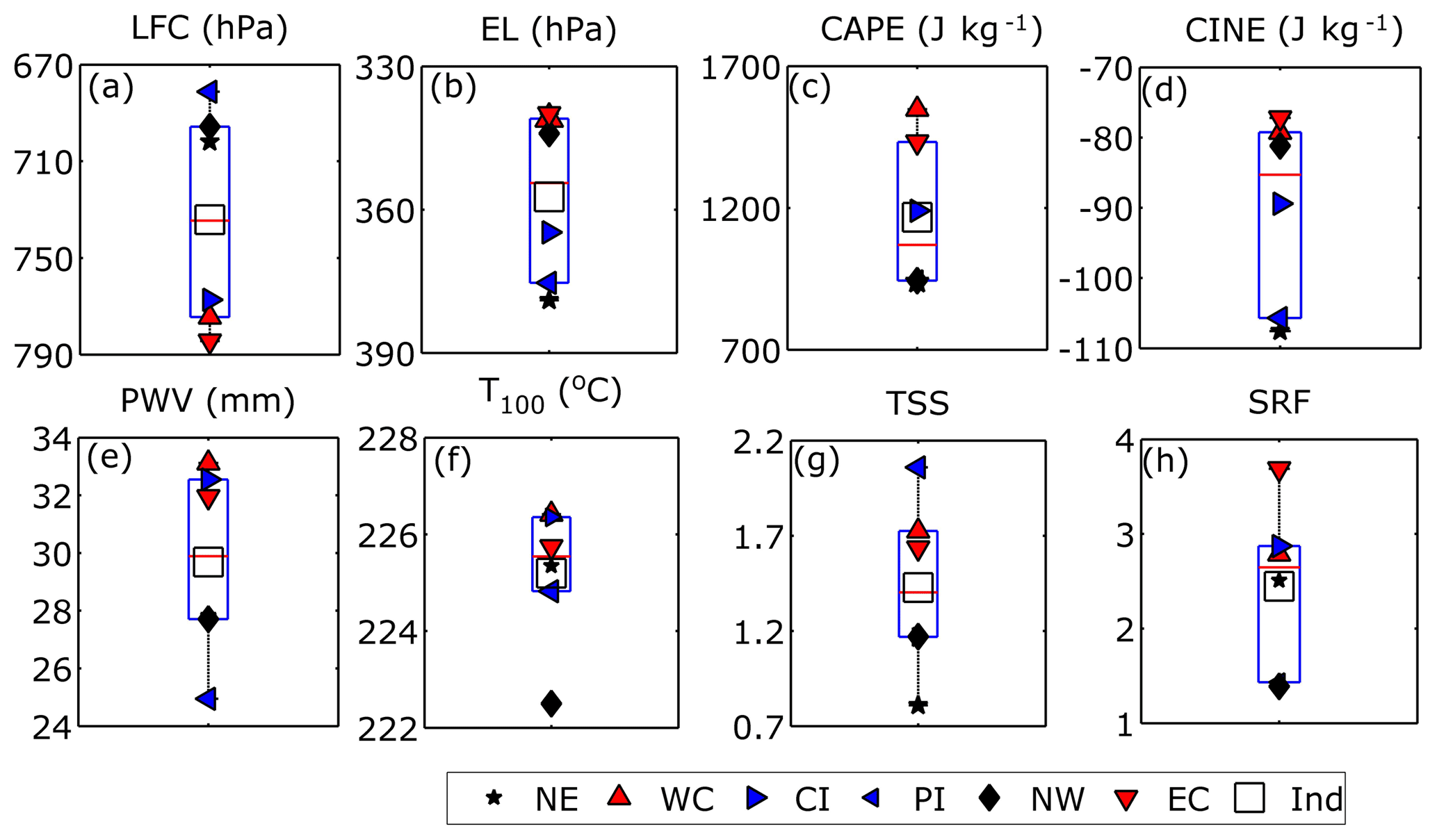
Figure 4Climatological mean values of (a) LFC, (b) EL, (c) CAPE, (d) CINE, (e) PWV, (f) T100, (g) TSS, and (h) SRF over the six subdivisions of India. Coastal regions are represented by red cones, the north-eastern and western regions are denoted by black stars and diamonds, and the blue cones represent the inland regions. Here the box limits refer to the upper and lower quartiles (25 % and 75 %), while the whiskers refer to the outlier limits of the data (5 % and 95 % limit of the population).
3.2 Climatological average of parameters
The climatological mean values of all instability parameters over six different Indian subdivisions are shown using box plot analysis (McGill, 1978) in Figs. 4 and S3. The utility of using this approach is that it will reveal which regions of India show normal expected variation (if it lies within the box limits, signifying 25 %–75 % percentage of the distribution), while on the other hand it will also identify those regions with extreme outlier values (lying outside the whiskers, signifying the outermost 5 % of the distribution). The LCL (Fig. S3a) and LFC (Fig. 4a) are found to be at the lowest altitudes in the coastal regions. As these stations receive most of the moisture from the sea, the EL (Fig. 4b) is also expected to be higher in the coastal areas and lower elsewhere. However, due to low moisture availability, the inland regions experience weaker instability, which results in lower CAPE (∼900 J kg−1) (Fig. 4c) with higher CINE (Fig. 4d) and WSH (Fig. S3f). During strong convection, the values of LI (Fig. S3b) (which represents the mid-tropospheric instability) are also expected to be more negative in the coastal regions. Similarly, height integrals of instability such as CAPE (Fig. 4c) and MLC (Fig. S3d) are significantly higher (∼1500 J kg−1) in the coastal regions, while the magnitude of MLC (Fig. S3d) is found to be almost half of CAPE. As the trends in total convective strengths below 300 hPa are quite low compared to that over the total atmospheric column, it follows that the portion of buoyant column above 300 hPa must have contributed significantly to the total convective developments over the Indian region. Again, being opposite of CAPE, CINE values are minimum in the coastal regions compared to inland and continental regions, thereby serving as a potential cause for the reduced instability in these regions.
Similar to the CAPE and MLC combination, the PWV (Fig. 4e) and PWL (Fig. S3e) pair shows the highest averages in the coastal regions due to their closest proximity to the adjoining seas. Also, PWL (moisture integral up to 700 hPa) is found to be almost half of PWV; hence the mid- and upper-tropospheric humidity is found to play a strong role in modulating the convective systems over India. The instability and moisture are highest in the coastal regions; hence the frequency of severe thunderstorms and rainfall is comparatively higher (Fig. 4g, h). The North West region shows the largest values of thunderstorm frequency, which is not supported by other parameters. Hence, it may be inferred that this is due to frequent dry storms called “Andhi”, which have no relation with convective instability and rainfall (Rajpal and Deka, 1980). Thus, it can be concluded that the effect of convection is large in the coastal regions compared to other regions, which resulted in high CAPE with more thunderstorms and intense rain occurrences.

Figure 5Long-term variation of (a) LFC, (b) EL, (c) CAPE, (d) CINE, (e) PWV, (f) T100, (g) TSS, and (h) SRF over the six subdivisions of India during the period 1980–2016. Legends are the same as in Fig. 4.
3.3 Long-term trends in the instability parameters
The long-term trends are calculated for each parameter during the entire study period of 1980–2016 for all regions using the robust regression analysis at a 95 % confidence interval as depicted in Figs. 5 and S4. For simplicity, the average trends along with their standard deviation values are depicted in Table 1. Also to investigate the significance of trend values calculated from these time series datasets, a t-test analysis (Gosset, 1908) is done on all parameters and locations. The p values are calculated at 95 % confidence limits for test analysis on all instability parameters over the Indian subdivisions, and interestingly, all the values are found to be below 0.05. Hence the time series variations to be presented in subsequent sections will always be statistically significant in nature. So, to have a better quantitative measure of the trend significance, the total changes in each of these parameters are presented in percentage form in place of the p values in the table. This process will enable an easy identification of regions experiencing more accelerated convective growth. But on the other hand, while analyzing the results of the trend analysis in statistical form, the absolute trend has to be given more importance as the percentage changes completely depend on the magnitude of the long-term mean. The LCL (Fig. S4a) height is found to decrease, which may lead to an overall increase in the number of rain occurrences throughout the country (provided that the amount of atmospheric instability is adequate). Conversely, the LFC (Fig. 5a) is found to ascend in all regions except NE, resulting in the reduction of lower-level instability and an increase of CINE magnitude (Fig. 5d). However, the extent of change in LFC (Fig. 5a) and LCL (Fig. S4a) is smallest in the coastal regions (∼10 hPa). In the case of the EL (Fig. 5b), a very prominent ascent is depicted in all regions (highest in coastal regions), which increases the height of the buoyant column; hence the net effect on total instability and CAPE (Fig. 5c) is expected to increase significantly. Similarly, LI (Fig. S4b) values become more negative in all the regions, with slightly higher magnitudes in the coastal regions. VT represents the lower-level atmospheric instability and hence is expected to be affected by the elevation in LFC. Thus, a reduction in VT (Fig. S4c) is seen, with minimum values in the coastal regions (∼0.3), medium in the NE and NW regions (∼0.5), and high in deep inland regions such as CI and PI (∼0.8). An intensification in CAPE (Fig. 5c) is seen in all regions (∼1100 J kg−1) as expected from EL (Fig. 5b) and LI. However, the increase is the highest (∼100 %) in the coastal regions, whereas in MLC (Fig. S4d), which is measured only up to the 300 hPa level, the increment is only 20 % of that in CAPE. Hence, it follows that the maximum contribution towards the increase in CAPE comes above 300 hPa. In the case of CINE, an overall enhancement in values is observed as expected (∼60 J kg−1). In addition, the trend values suggest a 2-fold increase of CINE in inland regions, while the values are much less (50 %) in the coastal regions due to a balancing effect from strong convection and CAPE in those regions.
The PWV (Fig. 5e) and PWL (Fig. S4e) values are increasing similarly to CAPE and MLC. The long-term trends in PWV are about 10 % of its climatological average, with the highest values in the coastal regions. Further, the lower-level moisture content of PWL (up to 700 hPa) showed an increase, but the trend values are comparatively smaller (∼6 %). Hence it follows that it is not the lower tropospheric moisture (below 700 hPa) but the remaining amount which is increasing significantly for all regions. Now, as this growth in upper-tropospheric moisture is analogous with a parallel rise in upper-level CAPE, there could be a possible association between these two factors, which needs to be investigated. The WSH (Fig. S4f) parameter increases in all regions of the country, and hence it produces an inhibiting effect on the lower-level instability. An upper-tropospheric cooling trend is observed in all other regions (Fig. 5f), with minimum values in the inland regions and maximum in the coastal regions. Consequently, the increase in CAPE values is maximum in the coastal regions and less elsewhere. The ordinary thunderstorm frequency is also found to increase (Fig. S4g), which may be due to the partial damping effect of an elevated LFC and CINE on lower-level instabilities. However, the TSS (Fig. 5g) are found to increase at a much higher rate compared to TSO, especially in the coastal regions. On the other hand, an increase in CINE and decrease of VT lead to an increase in the occurrence of WRF (Fig. S4h). However, due to a rise in CAPE and TSS (Fig. 5g), SRF (Fig. 5h) is also found to rise significantly by about 20 %, particularly in the coastal regions. It may be noted that, as EL has a more dominant effect on CAPE,the rise in SRF is much larger than that WRF (5 %). Finally, the long-term trends have been compared between the east and west coastal regions, and it is observed that the rate of increase in total instability is the most prominent in the western coast, while factors related to ascending LFC, CINE and reducing VT are more significant in Central India, which is the farthest from both the coasts. Thus, the long-term analysis infers that lower atmospheric instability reduced while the upper-tropospheric instability and moisture increased drastically over the Indian region. As a result, convective severity as expressed in terms of CAPE, TSS and SRF is increasing more strongly in the coastal regions, while in the continental areas this effect is dampened due to the contribution of increasing CINE and WSH.
3.4 Seasonal effect on long-term trends in the instability parameters
The seasonal variation of the long-term variations of atmospheric instability is shown in Figs. 6 and S5. LCL shows a uniform descent by 10 hPa in all seasons (Fig. S5a), whereas LFC ascends in most of the regions and seasons (Fig. 6a). However, this ascent is more prominent in the monsoon and post-monsoon season. However, the seasonal variation is absent in EL and LI (Figs. 6b, S5b), which are mainly associated with an upper-layer phenomenon. VT shows the most prominent reduction in monsoon and post-monsoon seasons (Fig. S5c). MLC and CAPE show a lot of regional disparities but with a common increase in its value in all the seasons (Figs. 6c, S5d). In monsoon and post-monsoon seasons, the increase in CAPE is slightly less due to the effect of decreasing VT and elevated LFC. CINE is closely related to VT and LFC; hence it shows a slight increase (of magnitude) in the monsoon and post-monsoon seasons, with maximum values in inland regions as expected (Fig. 6d).

Figure 6Seasonal trend of long-term variation for (a) LFC, (b) EL, (c) CAPE, (d) CINE, (e) PWV, (f) T100, (g) TSS, and (h) SRF over India during all seasons. Seasons are denoted as follows: (1) pre-monsoon (March–May), (2) monsoon (June–September), (3) post-monsoon (October–November), and (4) winter (December–February). Legends are the same as in Fig. 4.
PWV, PWL, and WSH represent a prominent increase in the monsoon followed by the post-monsoon (Fig. 6e, S5e–f). T100 is related to an upper-atmospheric phenomenon; hence no seasonal or spatial variation is displayed, except for a small cooling effect in pre-monsoon (Fig. 6f) due to the prevalence of intense convections events, which is supported by the strongest increase in CAPE. A decrease in lower atmospheric instability and increase in CINE is observed; hence TSO and WRF are expected to increase. However, this increase is only found to be more dominant in the monsoon and post-monsoon season (Fig. S5g, h). Another interesting result is that TSS and SRF do not behave similarly. TSS increase almost uniformly in all seasons, with the highest values in the pre-monsoon season. However, SRF increases mainly in the monsoon followed by the post-monsoon season (Fig. 6g, h). The observed disparity between them is due to the significant moisture availability during monsoon and post-monsoon seasons compared to the pre-monsoon period.
Further, in seasonal trends, east and west coasts show equivalent trends in all instability parameters, while =Central India still remains the region which is most affected by the ascension of LFC and CINE. Thus, the seasonal analysis reveals that the yearly long-term trends are almost uniformly distributed in all the seasons. The ordinary and weak thunderstorm frequencies show the strongest increase during monsoon and post-monsoon seasons, while the upper-atmospheric instability shows a weak influence in the pre-monsoonal trends on the yearly climatology.
3.5 Effect of specific periodicities on long-term trends
In the case of both annual and seasonal trend analysis, all Indian subdivisions are found to follow similar behavior. Hence, to find out the periodicities in the average long-term trends, the time series of all regions are averaged and then subjected to the EMD technique, which reveals the existence of four main periodicities, namely 1.5–2.5 years, corresponding to the QBO, 4–6 years, corresponding to ENSO, 10–12 years, corresponding to the solar cycle, and 16–20 years. A similar multi-decadal climatic oscillation was also reported by Dhaka et al. (2010). Hence for simplicity, this periodicity has been renamed as the Multi-decadal Climatic Oscillation (MCO).
The climatic trends of these periodicities for each parameter are calculated from robust regression analysis. An illustration of the obtained MCO periodicities for CAPE along all the Indian regions is shown in Fig. S2. Further for comparison, the trend values from each periodicity are normalized to percentages with respect to the total trend values for each parameter, and the net contributions of these individual periodicities are depicted in Figs. 7 and S6. The figure suggests that ENSO, QBO and the solar cycle have no effect on LCL (Fig. S6a), while MCO is quite strong. LFC shows minimal effects in all periodicities except the solar cycle period, which may be due to solar–terrestrial heating (Fig. 7a). EL and LI are significantly affected by both solar and MCO periodicities (Figs. 7b, S6b). But in LI, the contribution from MCO is much more than the solar effect. In the case of VT (Fig. S6c) the effects of both ENSO and MCO are found to be prominent. CAPE is found to be strongly influenced by MCO followed by the solar effect (Fig. 7c), and this is also discernible from the most strong increasing trends in CAPE, especially in the coastal regions after the years 1996–2000 in Fig. S2. However, in the case of MLC, the contribution of MCO is comparatively lesser (Fig. S6d); hence some separate phenomena above 300 hPa may have a prominent influence on increasing CAPE. Apart from CAPE, the effect of MCO is also found to be very strong in the case of CINE (Fig. 7d).
The moisture parameters like PWV and PWL show similar variability as in CAPE and MLC which only indicates significant moisture transport changes above 300 hPa in the past 18 years (Figs. 7e, S6e). WSH does not show the dominance of any periodicity (Fig. S6f), while T100 shows the most prominent contribution from the MCO (Fig. 7f), thereby showing its connection with the long-term variability in EL and CAPE with associated thunderstorm severity in recent years. TSO and TSS are both affected by the solar cycle and MCO (Figs. S6g, 7g), but TSS show that the effect of MCO is higher compared to TSO. Finally, the effect of MCO is also found to be more prominent in the case of SRF and WRF (Figs. 7h, S6h). In a nutshell, the MCO acts as the most dominant periodicity which has influenced the convective severity over India. So, in the coming sections, the MCO trends for both halves of 37 years will be studied. For ease of indication and referencing, these trends of an 18-year span each will be hereafter referred to as quasi-bi-decadal trends (since both spans are close to 20 years in length).
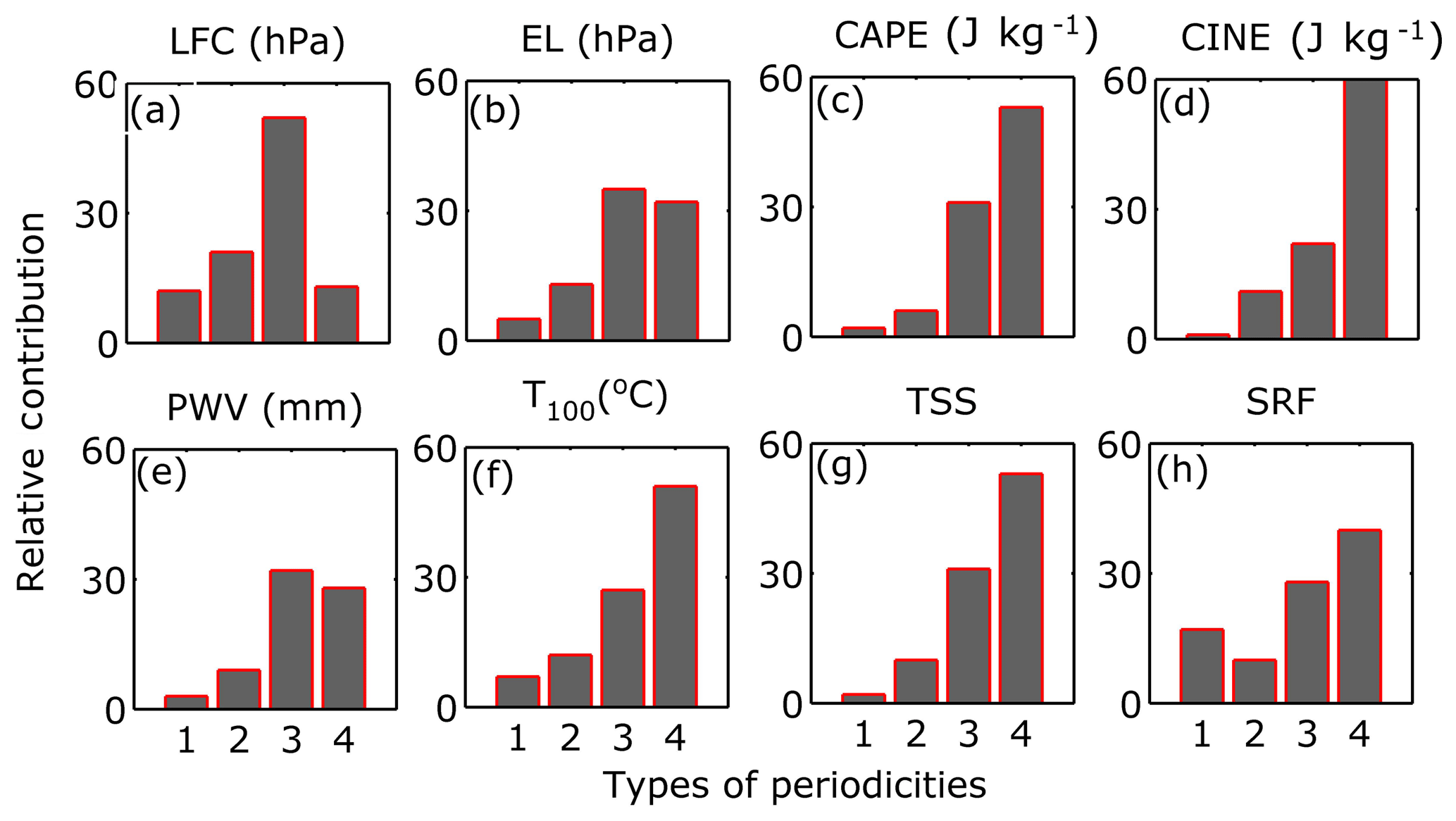
Figure 7Percentage contribution of various periodicities to the long-term trend of all instability parameters over India, namely (1) 1.5–2.5-year periodicity, (2) 4–6-year periodicity, (3) 10–12-year periodicity, and (4) 16–20-year periodicity.
3.6 Investigation of quasi-bi-decadal trends between 1980–1997 and 1999–2016
In the previous section, the annual averaged time series of many parameters such as EL, LI, VT, CAPE, CINE, T100, TSS, WRF, and SRF showed very significant changes with respect to MCO. It has also been indicated from Fig. S2 that the climatic trends before and after the period 1996–2000 are significantly different from each other. Therefore, the trends have been estimated with respect to two time periods before and after the year 1998. The time series for both MCO are produced, and their trend values are represented in Figs. 8 and S7. For simplicity, the MCO is referred to as C1 (1980 to 1998) and C2 (1999 to 2016), respectively. Starting with LCL, in C1 there is almost no change, but in C2 there is a strong descent, which influences the overall change in the time series (Fig. S7a). In the case of LFC, C1 shows an ascending trend, but in C2, a significant increasing pattern of LFC pressure is seen; hence an overall descent is obtained (Fig. 8a). An ascent in the EL is noticed in both the periods; however during C2 the trends show significant enhancement (Fig. 8b). The absolute magnitude of LI shows a slight reduction in C1 followed by a prominent increase in C2, resulting in a net increase in instability (Fig. S7b). VT shows an overall decreasing pattern in both the periods (Fig. S7c). CAPE (Fig. 8c) shows an enhancement in both the cycles, but the trends become more prominent in C2 (1500 J Kg−1). Similar to CAPE, MLC (Fig. S7d) also shows an increasing trend in both the cycles, but the trend values are also much smaller than in CAPE. Hence, the rise in EL height can be considered as a primary factor for increase in CAPE above 300 hPa during C2. CINE shows an increasing trend in both C1 and C2, but again the trend values are much stronger (∼80 J kg−1) during C2, especially in the inland regions (Fig. 8d).
The moisture trends in both PWV and PWL have shown a constant increase in both C1 and C2 throughout India (Figs. 8e, S7e). The WSH (Fig. 8k) also increases uniformly in both C1 and C2, with the strongest trends in the inland regions. A prominent cooling of ∼1.5∘ is seen in 100 hPa levels everywhere in C1, but in C2 the trend increases to ∘ (Fig. 8f), which can be considered responsible for the abrupt elevation in EL and increasing CAPE values during recent years. TSO increase slightly in C2 compared to C1 (Fig. S7g). But in the case of TSS, the positive trend gets doubled in C2, mainly in the coastal regions (Fig. 8g). Finally, in the case of SRF the trend values in C2 are slightly higher, with the maximum magnitudes in the coastal regions as expected (Fig. 8h). A further comparison between the six regions reveals that the west coast shows the maximum enhancement in all the instability and convective severity parameters in the past 18 years due to strong growth in moisture content and associated cooling at 100 hPa.
Conversely, during C2 Central India suffers from the maximum reduction in lower-level instability as seen from the rise in CINE and LFC due to the dearth of moisture content. Similar results are also found in other coastal and inland regions. Hence it follows that mainly during C2, the upper-tropospheric instability has enhanced everywhere, while the lower tropospheric instability has reduced, which has led to the development in both CAPE and CINE. As a result, both TSS–TSO and WRF–SRF combinations increase.
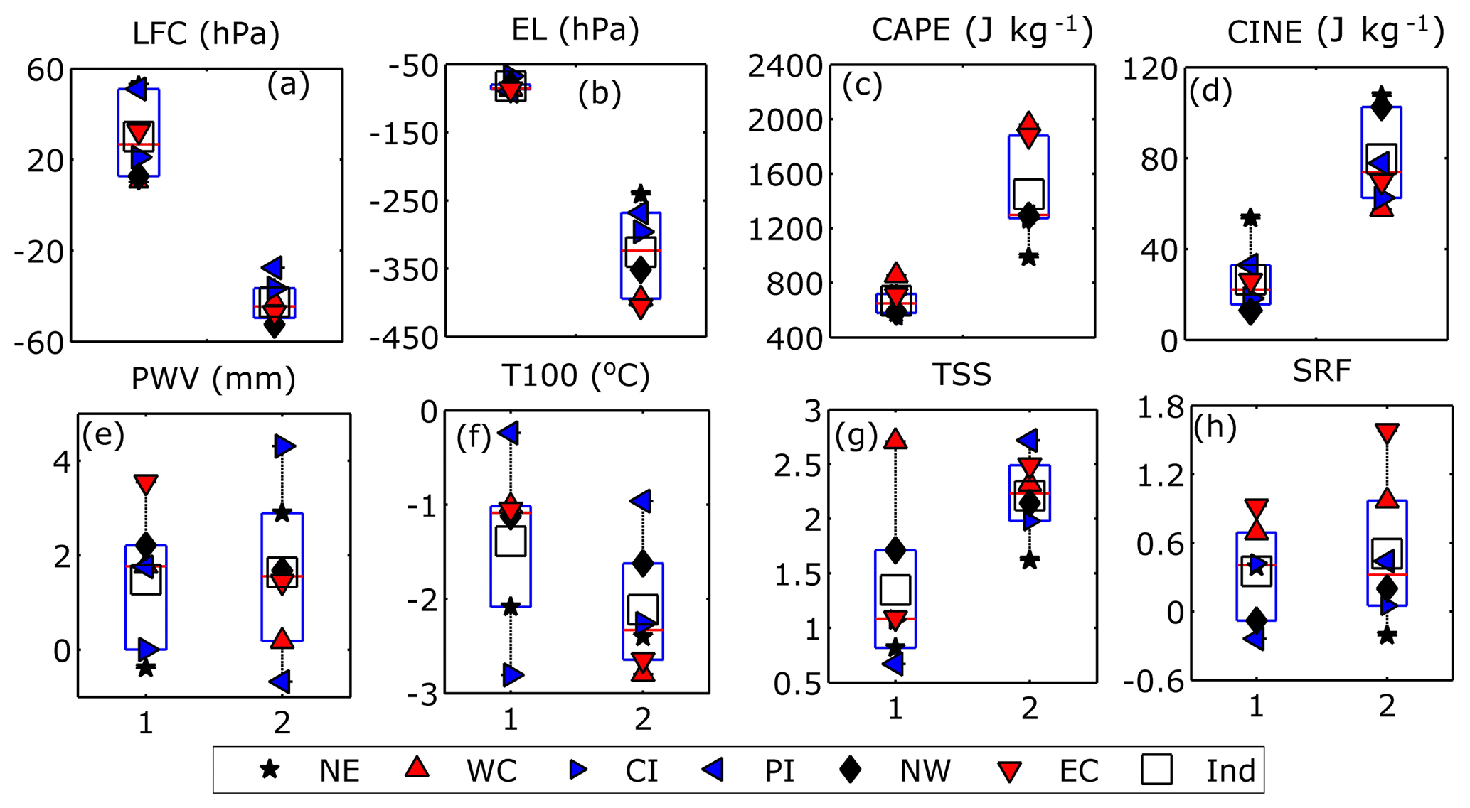
Figure 8Comparison of average values for two time periods indicating the trend of various instability parameter over the six subdivisions of India in two half periods of 18 years each (the numbers 1 and 2 represent the first and second period, C1 and C2, during 1980–1997 and 1999–2016, respectively) during 1999–2016. Legends are the same as in Fig. 4.

Figure 9Average values and climatological trends of specific humidity, ozone mixing ratio at 100 hPa and downward longwave radiation flux (DLWRF) with Absorptive Aerosol Index (AAI) over the six subdivisions of India over two half periods of 18 years each (1980–1997 and 1999–2016). Legends are the same as in Fig. 4.
From the previous section, it is inferred that a cooling trend at 100 hPa levels has led to the ascent in the EL ,which results in an increase in CAPE, TSS, and SRF. To explain the reason behind this, we consider the ozone to be a primary heating agent by absorbing the incoming solar ultraviolet radiation near the 100 hPa level (Mohanakumar, 2008). OH hydroxyl radicals are formed by oxidation of water vapor molecules by a reactive oxygen atom at the same height. On the other hand, it has been reported by Forster et al. (2007) that in recent years there has been a cooling in the upper troposphere due to a decrease in ozone concentration near 70 hPa. Hence, it is hypothesized that the OH radicals formed from the oxidation of water vapor can take an active role in the breakup of ozone molecules at 100 hPa levels, which may lead to this cooling effect. The preceding sections have shown a significant increase in moisture content especially in the coastal areas, hinting towards more moisture transport from the adjoining seas. Again, an increase in LI and CAPE values has also been reported in most of the regions, which can lift the available moisture to upper-atmospheric levels (Das et al., 2016; Guha et al., 2017). To add to this increasing CAPE and LI, many recent researchers have reported a net increase in the Hadley cell and Brewer–Dobson circulation strength (Liu et al., 2012; Fu et al., 2015; Shepherd and McLandress, 2011), which also assists in the uplift of moisture to upper-atmospheric levels. Thus, it is inferred that low-level moisture is transported to the upper troposphere and above, where it is responsible for ozone depletion and cooling, thereby elevating the EL and increasing the thunderstorm severity.
To test this hypothesis, yearly averaged time series of specific humidity and ozone mixing ratio data are collected for all stations and the quasi-bi-decadal trend values are depicted in Fig. 9. This figure shows a rise in specific humidity levels by 7 % in C2 over the whole of India (Fig. 9a). On the other hand, trends of specific humidity have almost trebled in C2 phase, with the maximum values in the coastal regions (Fig. 9e). As water vapor concentration increases, ozone concentration is expected to decrease. The ozone trends support this hypothesis by showing a sharp transition from low positive to high negative values during C2 (Fig. 9b, f). It may be additionally noted that the specific humidity increase and reduction in ozone content are strongest in the coastal regions, leading to a higher increase in CAPE and severe thunderstorms in those regions.
In recent decades, the Indian region has experienced a surface warming trend, which is mainly caused by an increase in greenhouse gas (GHG) concentrations, as pointed out by Basha et al. (2017). These GHGs are heat-absorbing in nature and these particles reside within the lower troposphere (generally below 700 hPa) due to surface heating and boundary layer dynamics as reported by Chakraborty et al. (2017b). Further, these gases has a tendency to absorb and then re-emit the outgoing longwave radiation as emitted by the Earth, resulting in more downward longwave radiation flux and atmospheric heating, which elevates the LFC. Additionally, this near-surface heating reduces the vertical temperature lapse rate, leading to a drop in lower instability (VT). To test this hypothesis, the yearly averaged downward longwave radiation flux (DLWRF) time series is depicted over the Indian region in Fig. 9c and g, which also suggest that DLWRF values are increasing in C2. To show that the increase in DLWRF is due to the heat-absorbing particles only, the trends in Absorbing Aerosol Index (AAI) are shown for all the regions. The figure suggests that the mean of AAI is increasing slightly more in C2 with a positive trend (Fig. 9d, h). Due to this heating of lower atmosphere and capping of lapse rates by GHGs and absorptive aerosols, the LFC starts ascending, so WSH and CINE get stronger while VT reduces. As a result, the ordinary to weak convective occurrences start increasing.
Finally, it has to be explained why the upper-air instability and CAPE are mainly increasing in the coastal regions. The coastal regions have high moisture content (Saha et al., 2017). Because of the strong land–ocean contrast, low-level winds close to 850 hPa flow into the coastal regions and disperse the pollutants and GHGs to other locations, leading to a weaker convective inhibition in those areas. This hypothesis is supported by the lowest AAI values in the coasts despite having high increasing trends in those areas. In addition, the ample moisture supply in the coastal regions is lifted up to the upper troposphere and lower stratosphere (UTLS), where it undergoes prominent cooling due to ozone reduction. Hence, the EL ascends more, resulting in higher CAPE, which finally led to an abrupt rise in TSS and SRF in the coastal regions. However, in the inland regions the layer of absorptive aerosols and GHGs cannot be dispersed amply due to the dearth of strong lower-level winds. As a result, the growth of lower atmospheric instability gets inhibited in the inland regions. Further, due to less moisture availability, UTLS cooling and EL ascent are much lower; hence there is less of a rise in CAPE, which ultimately leads to an increase in TSO and WRF in those subdivisions. It may be noted that the trend in AAI is not significantly different for the two time periods C1 and C2. Again, it is the EL and not the LFC or LCL which influences CAPE strongly; hence the strong trends of humidity increase and ozone reduction overpower the weaker inhibitory effect from the atmospheric aerosols, and this acts as a major driving force behind the increase in convective severity compared to most of the cases.
In recent decades, global warming has become a threat to human life and society in terms of its various implications. An increase in surface temperature leads to stronger atmospheric instabilities, which in turn may increase the CAPE, resulting in more severe thunderstorm and precipitation activity. Hence, the long-term variations of instability parameters will help to better understand the changes in the weather extremes with respect to climate change. In light of the above, the main objective of the present study is to analyze whether convective instability has changed over the Indian region during the last 37 years and then to find its possible effects on thunderstorm and rainfall severity. Radiosonde measurements from Integrated Global Radiosonde Archive (IGRA) pertaining to 27 stations across six Indian subdivisions are utilized to depict the spatial distribution of these long-term trends during the period of 1980–2016. The selection of instability parameters is done based on principal component analysis (PCA), which showed the importance of investigating LI and VT further. A total of 16 parameters (including parcel and instability data with moisture content, wind shear, and thunderstorm and rainfall frequencies) have been utilized. A robust fit approach is employed on the regional average time series to calculate the long-term trends on both a yearly and a seasonal basis. The main highlights obtained from the present study are listed below:
-
The coastal regions experience the most significant rise in convective available potential energy (CAPE) and equilibrium level (EL), leading to more occurrences of severe thunderstorms (TSS) and severe rainfall (SRF), while the inland regions undergo a decrease in lower atmospheric instability due to elevated convective inhibition energy (CINE) and level of free convection resulting in more ordinary thunderstorms (TSO) and occurrences of weak rainfall (WRF).
-
In the pre-monsoon season, an increasing activity of TSS is observed due to higher instability connected to increasing EL height and CAPE values, along with a decrease in LI values, while the monsoon and post-monsoon season experiences more prominent ascension in LFC height, with larger values of CINE and wind shear (WSH), thereby increasing the tropospheric stability, which leads to increased TSO and occurrences of WRF all over the Indian region.
-
The Empirical Mode Decomposition (EMD) analysis on the instability parameters reveals that the 16–20-year Multi-decadal Climatic Oscillation (MCO) is the most dominant component in all six Indian subdivisions.
-
The quasi-bi-decadal analysis reveals an increase in magnitude in many parameters like EL, CAPE, CINE, TSO, and TSS along with cooling at the 100 hPa level during C2 (1999–2016), which dominates the 37-year trend.
-
The annual and quasi-bi-decadal trends support the finding that the increase in thunderstorm severity and associated convection is strongest along western coast due to maximum moisture ingress from the sea, while the greatest reduction in lower atmospheric instability is experienced in Central India, owing to the lack of pollutant dispersal as it is situated very far from the sea.
-
In the coastal regions, an ample amount of water vapor is advected into the middle troposphere from the surrounding seas, which in the presence of strong uplift goes up to the upper troposphere and lower stratosphere (UTLS) where ozone depletion occurs, leading to a strong cooling effect. This cooling effect enables the ascent in EL, resulting in much stronger LI and CAPE values and hence more TSS and SRF.
-
In the inland regions, the dispersing effect by sea winds is absent; hence the capping effect of lower instability is greater, leading to stronger CINE values. Again, due to the dearth of moisture transport from the seas, the UTLS cooling is less, leading to a weaker rise in CAPE; consequently, the frequencies of TSO and WRF increase significantly.
-
However, as the ascent in EL has a stronger contribution over increasing CAPE than the inhibitory effect of LFC, the long-term trends are expected to be more strongly influenced by the ozone decomposition and cooling at 100 hPa levels than the capping effect of low-level inversions from absorptive aerosols; hence the convective severity over the Indian regions is found to increase.
Thus, it may be inferred that in the near future also, convective severity will increase strongly in the coastal regions, while weak and ordinary thunderstorms will be more common in the inland regions. It may appear in certain sections of this analysis that the trends of CAPE and EL are exorbitantly high, but this is not the actual case because previous studies by Murugavel et al. (2012) and Gettlemann et al. (2002) have also shown almost comparable trends in convective severity both in India and abroad. Nevertheless, this study has an advantage over previous approaches as it successfully explains the hypothesis brought forward by early research attempts that UTLS cooling at 100 hPa and GHGs' concentration rise can regulate the climatic trends of convective severity and frequency, especially over tropical regions in the recent decades.
After going through the study, there may be a possibility of thinking that the change in instability trends is due to the change in sensors around 1998. But this is not the actual case because, first, there has not been any mention in past literature surveys related to any change in radiosonde data quality during the late 1990s in IMD or IGRA. Secondly, the yearly variations of all 16 parameters for various IGRA stations as in Chennai do not commonly show any abrupt change in time series during 1996–2004 except for a few cases. Thirdly, it has been revealed by IMD reports that the year 2000 was a tipping point for the climate-change-led warming over India, thereby leading to a rise in catastrophic weather events. A cataclysmic fallout will follow by the year 2040 if these emission scenarios are not curbed soon (Hindustan Times, 2019). Thus, it follows that the observed changes in the atmospheric instability trends before and after 1996–2004 are due to a synoptic global-warming-based climate change phenomena and not due to any change in radiosonde sensor type.
However, in spite of all this, the present study has certain shortcomings. The most important one among them is that this set of explanations is based on isolated information from selected in situ observations, and hence it needs to be studied in more detail spatially in future using model-based observations. In recent years, certain studies have utilized multiple global circulation model (GCM) outputs over the US to infer the robust increase in thunderstorm frequency (Diffenbaugh et al., 2013; Seeley and Romps, 2015). However, these types of studies have not yet been done over the Indian region. Hence, a combination of multi-station radiosonde data with model data will be utilized to provide a generalized picture about convective severity over the Indian region. Additionally, this study also introduces the effect of direct aerosol heating on instability and convection, but the probable impact of indirect aerosol loading on modulating the cloud lifetime and convective severity has not been discussed here. This is because the relationship between indirect aerosol forcing and instability is still unclear and complex (Connoly et al., 2013). A few research studies in recent years have hypothesized that a higher concentration of aerosols may lead to stronger updraft velocities by altering the latent heat release resulting in growth of CAPE and TSS (Tao et al., 2012; Storer and van den Heever, 2013). However, this is a season- and location-specific phenomenon, and hence it is not expected to impact the yearly trend of CAPE and TSS as strong as the upper-tropospheric cooling effect projected in this study. But in future, an exhaustive analysis of cloud and aerosol components involving both in situ and modeled data can be done to investigate its contribution to the total trends of CAPE, TSS, and SRF over the Indian region.
Data used in present study can be obtained directly from the IGRA website.

The supplement related to this article is available online at: https://doi.org/10.5194/acp-19-3687-2019-supplement.
RC performed complete analysis and wrote the first draft. MVR provided the initial concept, guidance, and editing, and SGB contributed to analysis, discussion, and editing.
The authors declare that they have no conflict of interest.
One of the authors (Rohit Chakraborty) thanks the Science and Engineering Research Board, Department of Science and Technology, for providing a fellowship under the National Post-Doctoral Scheme (File No:PDF/2016/001939). He also acknowledges the National Atmospheric Research Laboratory for providing necessary support and data for this work. The authors also thank Sivan Thankamani Akhil Raj, Sanjeev Dwivedi, and Nelli Narendra Reddy for their suggestions.
This paper was edited by Michael Pitts and reviewed by three anonymous referees.
Alappattu, D. P. and Kunhikrishnan, P. K.: Premonsoon estimates of convective available potential energy over oceanic region surrounding Indian subcontinent, J. Geophys. Res.-Atmos., 114, D08108, https://doi.org/10.1029/2008JD01152, 2009.
Ananthakrishnan, R.: Some aspects of the monsoon circulation and monsoon rainfall, Pure Appl. Geophys., 115, 1209–1249, 1977.
Andersen, R.: Modern methods for robust regression, 152, Quantitative Applications in Social Sciences, Sage, Thousand Oaks, California, USA, 2008.
Basha, G., Kishore, P., Ratnam, M. V., Jayaraman, A., Kouchak, A. A., Ouarda, T. B. M. J., and Velicogna, I.: Historical and Projected Surface Temperature over India during 20th and 21st century, Sci. Rep., 7, 2987, https://doi.org/10.1038/s41598-017-02130-3, 2017.
Basha, G. and Ratnam, M. V.: Moisture Variability over Indian monsoon regions, Atmos. Res., 132–133, 35–45, 2013.
Basha, G., Ratnam, M. V., and Krishna Murthy, B. V.: Upper tropospheric water vapor variations, J. Earth Syst. Sci., 122, 1583–1591, 2013.
Brooks, H. E.: Severe thunderstorms and climate change, Atmos. Res., 123, 129–138, 2013.
Chakraborty, R. and Maitra, A.: Retrieval of atmospheric properties with radiometric measurements using neural network, Atmos. Res., 181, 124–132, https://doi.org/10.1016/j.atmosres.2016.05.011, 2016.
Chakraborty, R., Talukdar, S., Saha, U., Jana, S., and Maitra, A.: Anomalies in relative humidity profile in the boundary layer during convective rain, Atmos. Res., 191, 74–83, https://doi.org/10.1016/j.atmosres.2017.03.011, 2017a.
Chakraborty, R., Saha, U., Singh, A. K., and Maitra, A.: Association of atmospheric pollution and instability indices: A detailed investigation over an Indian urban metropolis, Atmos. Res., 196, 83–96, https://doi.org/10.1016/j.atmosres.2017.04.033, 2017b.
Chakraborty, R., Basha, G., and Ratnam, M. V.: Diurnal and long-term variation of instability indices over a tropical region in India, Atmos. Res., 207, 145–154, https://doi.org/10.1016/j.atmosres.2018.03.012, 2018.
Connolly, P. J., Vaughan, G., May, P. T., Chemel, C., Allen, G., Choularton, T. W., Gallagher, M. W., Bower, K. N., Crosier, J., and Dearden, C.: Can aerosols influence deep tropical convection? Aerosol indirect effects in the Hector island thunderstorm, Q. J. Roy. Meteor. Soc., 139, 2190–2208, https://doi.org/10.1002/qj.2083, 2013.
Das, S., Chakraborty, R., and Maitra, A.: A random forest algorithm for nowcasting of intense precipitation events, Adv. Space Res., 60, 1271–1282, https://doi.org/10.1016/j.asr.2017.03.026, 2017.
Das, S. S., Ratnam, M. V., Uma, K. N., Patra, A. K., Subrahmanyam, K. V., Girach, I. A., Suneeth, K. V., Kumar, K. K., and Ramkumar, G.: Stratospheric intrusion in to the troposphere during the tropical cyclone Nilam (2012), Q. J. Roy. Meteor. Soc., 142, 2168–2179, https://doi.org/10.1002/qj.2810, 2016.
De Graaf, M., Stammes, P., Torres, O., and Koelemeijer, R. B. A.: Absorbing Aerosol Index: Sensitivity analysis, application to GOME and comparison with TOMS, J. Geophys. Res.-Atmos., 110, D01201, https://doi.org/10.1029/2004JD00517, 2005.
Dhaka, S. K., Sapra, R., Panwar, V., Goel, A., Bhatnagar, R., and Kaur, M.: Influence of large-scale variations in convective available potential energy (CAPE) and solar cycle over temperature in the tropopause region at Delhi (28.3∘ N, 77.1∘ E), Kolkata (22.3∘ N, 88.2∘ E), Cochin (10∘ N, 77∘ E), and Trivandrum (8.5∘ N, 77.0∘ E) using radiosonde during 1980–2005, Earth Planets Space, 62, 319–331, 2010.
Diffenbaugh, N. S., Scherer, M., and Trapp, R. J.: Robust increases in severe thunderstorm environments in response to greenhouse forcing, P. Natl. Acad. Sci. USA, 110, 16361–16366, 2013.
Durre, I., Vose, R. S., and Wuertz, D. B.: Overview of integrated global radiosonde archive, J. Climate, 19, 53–68, 2006.
Emanuel, K.: Climate and tropical cyclone activity: A new model downscaling approach, J. Climate, 19, 4797–4802, 2006.
Ferreira, A. P., Nieto, R., and Gimeno, L.: Completeness of radiosonde humidity observations based on the IGRA, Earth Syst. Sci. Data Discuss., https://doi.org/10.5194/essd-2018-95, in review, 2018.
Forster, P. M., Bodeker, G., Schofield, R., Solomon, S., and Thompson, D.: Effects of ozone cooling in the tropical lower stratosphere and upper troposphere, Geophys. Res. Lett., 34, L23813, https://doi.org/10.1029/2007GL031994, 2007.
Fu, Q., Lin, P., Solomon, S., and Hartmann, D. L.: Observational evidence of the strengthening of the Brewer-Dobson circulation since 1980, J. Geophys. Res.-Atmos., 120, 10214–10228, 2015.
Gensini, V. A. and Mote, T. L.: Downscaled estimates of late 21st century severe weather from CCSM3, Climate Change, 129, 307–321, 2015.
Gettelman, A., Seidel, D. J., Wheeler, M. C., and Ross, R. J.: Multidecadal trends in tropical convective available potential energy, J. Geophys. Res.-Atmos., 107, 4606, https://doi.org/10.1029/2001JD001082, 2002.
Gosset, W. S.: The probable error of a mean, Biometrika, 6, 1–25, 1908.
Guha, B. K., Chakraborty, R., Saha, U., and Maitra, A.: Tropopause height characteristics associated with ozone and stratospheric moistening during intense convective activity over Indian sub-continent, Global Planet. Change, 158, 1–12, https://doi.org/10.1016/j.gloplacha.2017.09.009, 2017.
Hindustan Times: https://www.hindustantimes.com/environment/freak-weather-to-rise-in-india-over-two-decades/story-T1G8SgfBh8jydT15UnKGuM.html, last access: 24 January 2019.
Hotelling, H.: Analysis of complex statistical variables into principal components, J. Educ. Psychol., 24, 417–411, 1936.
Huntrieser, H., Schiesser, H. H., Schmid, W., and Waldvogel, A.: Comparison of Traditional and Newly Developed Thunderstorm Indices for Switzerland, Weather Forecast., 12, 108–125, 1997.
Integrated Global Radiosonde Archive Version 2 (IGRA2): provided by National Oceanic and Atmospheric Administration, USA, available at: https://www1.ncdc.noaa.gov/pub/data/igra/derived/derived-por/, last access: 18 March 2019.
Kharin, V. V, Zwiers, F. W., Zhang, X., and Wehner, M.: Changes in temperature and precipitation extremes in the CMIP5 ensemble, Climate Change, 119, 345–357, 2013.
Liu, J., Song, M., Hu, Y., and Ren, X.: Changes in the strength and width of the Hadley Circulation since 1871, Clim. Past, 8, 1169–1175, https://doi.org/10.5194/cp-8-1169-2012, 2012.
Manohar, G. K., Kandalgaonkar, S. S., and Tinmaker, M. I. R: Thunderstorm activity India and Indian southwest monsoon. J. Geophys. Res.-Atmos., 104, 4169–4188, 1999.
McGill, R., Turkey, J. W., and Larsen, W. A.: Variations of Box Plots, The American Staistician, Taylor and Francis, Milton Park, Oxfordshire, UK, 32, 12–16, 1978.
Mohanakumar, K.: Stratosphere-troposphere interactions: introduction, Springer Science Business Media, the Netherlands, 2008.
Murthy, B. S. and Sivaramakrishnan, S.: Moist convective instability over the Arabian Sea during the Asian summer monsoon, 2002, Meteorol. Appl., 13, 63–72, https://doi.org/10.1017/S135048270500201X, 2006.
Murugavel, P., Pawar, S. D., and Gopalakrishnan, V.: Trends of convective available potential energy over the Indian region and its effect on rainfall, Int. J. Climatol., 32, 1362–1372, 2012.
Narendra Reddy, N., Venkat Ratnam, M., Basha, G., and Ravikiran, V.: Cloud vertical structure over a tropical station obtained using long-term high-resolution radiosonde measurements, Atmos. Chem. Phys., 18, 11709–11727, https://doi.org/10.5194/acp-18-11709-2018, 2018.
Nelli, N. R. and Rao, K. G.: Contrasting variations in the surface layer structure between the convective and non-convective periods in the summer monsoon season for Bangalore location during PRWONAM, J. Atmos. Sol.-Terr. Phy., 167, 156–168, https://doi.org/10.1016/j.jastp.2017.11.017, 2018.
Pai, D. S., Sridhar, L., Rajeevan, M., Sreejith, O. P., Satbhai, N. S., and Mukhopadhyay, B.: Development of a new high spatial resolution (0.25×0.25) long period (1901–2010) daily gridded rainfall data set over India and its comparison with existing data sets over the region, Mausam, 65, 1–18, 2014.
Prein, A. F., Rasmussen, R. M., Ikeda, K., Liu, C., Clark, M. P., and Holland, G. J.: The future intensification of hourly precipitation extremes, Nat. Clim. Change, 7, 48–52, 2017.
Raipal, D. K. and Deka, S. N: ANDHI, convective dust storm of northwest India, Mausam, 31, 431–442, 1980.
Raj, S. T. A., Ratnam, M. V., Rao, D. N., and Murthy, B. V. K.: Long-term trends in stratospheric ozone, temperature, and water vapor over the Indian region, Ann. Geophys., 36, 149–165, https://doi.org/10.5194/angeo-36-149-2018, 2018.
Rajeevan, M., Bhate, J., Kale, J. D., and Lal, B.: High resolution daily gridded rainfall data for the Indian region: Analysis of break and active monsoon spells, Curr. Sci., 91, 296–306, 2006.
Rajeevan, M., Bhate, J., and Jaswal, A. K.: Analysis of variability and trends of extreme rainfall events over India using 104 years of gridded daily rainfall data, Geophys. Res. Lett., 35, 1–6, https://doi.org/10.1029/2008GL035143, 2008.
Rakshit, G., Chakraborty, R., and Maitra, A.: Effect of vertical wind on rain drop size distributions in the boundary layer, 2016 International Symposium on Antennas and Propagation (ISAP), 846–847, 2016, available at: http://ieeexplore.ieee.org/stamp/stamp.jsp?tp=&arnumber=7821528&isnumber=7821043 (last access: 18 March 2019), 2016.
Rao, Y. P.: Southwest monsoon, Synoptic Meteorology, New Delhi, 1976.
Riemann-Campe, K., Fraedrich, K., and Lunkeit, F.: A global climatology of convective available potential energy (CAPE) and convective inhibition (CIN) in ERA-40 reanalysis, Atmos. Res., 93, 534–545, 2009.
Saha, U., Maitra, A., Midya, S. K., and Das, G. K.: Association of thunderstorm frequency with rainfall occurrences over an Indian urban metropolis, Atmos. Res., 138, 240–252, 2014.
Saha, U., Chakraborty, R., Maitra, A., and Singh, A. K.: East-west coastal asymmetry in the summertime near-surface wind speed and its projected change in future climate over the Indian region, Glob. Planet. Change, 152, 76–87, https://doi.org/10.1016/j.gloplacha.2017.03.001, 2017.
Santhi, Y. D., Ratnam, M. V., Dhaka, S. K., and Rao, S. V.: Global morphology of convection indices observed using COSMIC GPS RO satellite measurements, Atmos. Res., 137, 205–215, 2014.
Seeley, J. T. and Romps, D. M.: The effect of global warming on severe thunderstorms in the United States, J. Climate, 28, 2443–2458, 2015.
Shepard, D.: A two-dimensional interpolation function for irregularly-spaced data, in: Proceedings of the 1968 23rd ACM national conference, New York, 517–524, 1968.
Shepherd, T. G. and McLandress, C.: A robust mechanism for the strengthening of the Brewer-Dobson circulation in response to climate change: Critical-layer control of subtropical wave breaking, J. Atmos. Sci., 68, 784–797, 2011.
Storer, R. L. and van den Heever, S. C.: Microphysical processes evident in aerosol forcing of tropical deep convective clouds, J. Atmos. Sci., 70, 430–446, https://doi.org/10.1175/JAS-D-12-076.1, 2013.
Tao, W. K., Chen, J. P., Li, Z., Wang, C., and Zhang, C.: Impact of aerosols on convective clouds and precipitation, Rev. Geophys., 50, RG2001, https://doi.org/10.1029/2011RG000369, 2012.
Wang, S.-Y., Davies, R. E., Huang, W.-R., and Gillies, R. R.: Pakistan's two-stage monsoon and links with the recent climate change, J. Geophys. Res.-Atmos., 116, 1–15, https://doi.org/10.1029/2011JD015760, 2011.
Webster, P. J., Holland, G. J., Curry, J. A., and Chang, H.-R.: Changes in tropical cyclone number, duration, and intensity in a warming environment, Science, 309, 1844–1846, 2005.
Wu, Z. and Huang, N. E.: Ensemble empirical mode decomposition: a noise-assisted data analysis method, Advances in Adaptive Data Analysis, 1, 1–41, 2009.
Xie, B., Zhang, Q., and Ying, Y.: Trends in precipitable water and relative humidity in China: 1979–2005, J. Appl. Meteorol. Clim., 50, 1985–1994, 2011.