the Creative Commons Attribution 4.0 License.
the Creative Commons Attribution 4.0 License.
 | 20 Mar 2019
The CAMS reanalysis of atmospheric composition
Melanie Ades
Anna Agustí-Panareda
Jérôme Barré
Anna Benedictow
Anne-Marlene Blechschmidt
Juan Jose Dominguez
Richard Engelen
Henk Eskes
Johannes Flemming
Vincent Huijnen
Luke Jones
Zak Kipling
Sebastien Massart
Mark Parrington
Vincent-Henri Peuch
Miha Razinger
Samuel Remy
Michael Schulz
Martin Suttie
The Copernicus Atmosphere Monitoring Service (CAMS) reanalysis is the latest global reanalysis dataset of atmospheric composition produced by the European Centre for Medium-Range Weather Forecasts (ECMWF), consisting of three-dimensional time-consistent atmospheric composition fields, including aerosols and chemical species. The dataset currently covers the period 2003–2016 and will be extended in the future by adding 1 year each year. A reanalysis for greenhouse gases is being produced separately. The CAMS reanalysis builds on the experience gained during the production of the earlier Monitoring Atmospheric Composition and Climate (MACC) reanalysis and CAMS interim reanalysis. Satellite retrievals of total column CO; tropospheric column NO2; aerosol optical depth (AOD); and total column, partial column and profile ozone retrievals were assimilated for the CAMS reanalysis with ECMWF's Integrated Forecasting System. The new reanalysis has an increased horizontal resolution of about 80 km and provides more chemical species at a better temporal resolution (3-hourly analysis fields, 3-hourly forecast fields and hourly surface forecast fields) than the previously produced CAMS interim reanalysis. The CAMS reanalysis has smaller biases compared with most of the independent ozone, carbon monoxide, nitrogen dioxide and aerosol optical depth observations used for validation in this paper than the previous two reanalyses and is much improved and more consistent in time, especially compared to the MACC reanalysis. The CAMS reanalysis is a dataset that can be used to compute climatologies, study trends, evaluate models, benchmark other reanalyses or serve as boundary conditions for regional models for past periods.
- Article
(21803 KB) -
Supplement
(1439 KB) - BibTeX
- EndNote


The European Centre for Medium-Range Weather Forecasts (ECMWF) has been producing atmospheric composition (AC) forecasts and analyses for over a decade. The model and data assimilation system used for this was developed as a European effort by a consortium of partners funded by several European Union (EU) projects. It began in 2005, with the EU-funded Global Monitoring for Environment and Security (GEMS) project (Hollingsworth et al., 2008) that built the capacity for a global and regional forecasting and data assimilation system of AC. In GEMS, ECMWF's Integrated Forecast System (IFS) was extended to allow for the data assimilation and modelling of aerosols, chemically reactive gases and greenhouse gases, and the first daily forecasts of reactive gases such as carbon monoxide (CO) and tropospheric ozone (O3) were made public in May 2007 (Flemming et al., 2017a). This was followed a year later, in July 2008, by the real-time data assimilation of aerosol optical depth (AOD; Benedetti et al., 2009) and selected reactive gases (Inness et al., 2013) in the daily GEMS system. The AC system was further developed in the earlier Monitoring Atmospheric Composition and Climate (MACC) projects (Flemming et al., 2015; Inness et al., 2015; Massart et al., 2014; Agustí-Panareda et al., 2014) between 2009 and 2014 and has been running fully operationally in the Copernicus Atmosphere Monitoring Service (CAMS), operated by ECMWF, since January 2015. In the rest of this paper we will refer to the system built in GEMS–MACC–CAMS as the CAMS system and focus on reactive gases and aerosols.
While the modelling components for aerosols were included directly in the IFS from the beginning of GEMS (Morcrette et al., 2009), the initial approach for the reactive gases was to build a “coupled system” where the chemical transport model (CTM) Model for OZone And Related chemical Tracers (MOZART), version 3.5 (Kinnison et al., 2007), was coupled to the IFS using the Ocean Atmosphere Sea Ice Soil (OASIS 4) coupling software (Flemming et al., 2009). Later, in the MACC projects, a modified version of the Carbon Bond 2005 chemistry scheme (CB05; Huijnen et al., 2010) derived from the CTM Transport Model 5 (TM5) was integrated in the IFS (referred to as IFS(CB05); Flemming et al., 2015), making the system more computationally efficient and improving the system's ability to represent interactions between meteorology and chemistry. In parallel with the model system, the use of observations in the data assimilation system also evolved with time as new datasets became available and satellite retrievals were improved.
The initial forecasts and analyses in 2007–2008 had a horizontal resolution of T159 (∼110 km). This was increased to T255 (∼80 km) in July 2012 and to T511 (∼40 km) in June 2016. The vertical resolution has so far always consisted of 60 model levels in the vertical, with the top level at 0.1 hPa. Details about the different model versions used over time are given in Table A1 in the Appendix. The continuing upgrades of the CAMS model and data assimilation system and the changes they brought with them made it difficult if not impossible to compare data from a recent period with earlier data in a meaningful way. For example, it was not possible to calculate seasonal anomalies or trends with a system that had changed so much over time. Therefore, so-called reanalyses were produced with the CAMS system, where a long time period was rerun with a single version of the model and data assimilation system, taking care to minimise changes in the versions of the used emissions or assimilated satellite retrievals. Such a system gives the temporal consistency needed to deduce trends (e.g. Flemming et al., 2017b) or to provide maps of annual or seasonal anomalies (e.g. Flemming and Inness, 2018).
Producing long reanalyses with a single model version is a well-known procedure in numerical weather prediction (NWP), and several weather centres have produced meteorological reanalysis datasets. It has long been an important activity at ECMWF (ERA-40, Uppala et al., 2005; ERA-Interim, Dee et al., 2011; ERA-5, Hersbach et al., 2018), and other meteorological centres such as National Centers for Environmental Protection (NCEP; CFSR; Saha et al., 2010), the Japan Meteorological Agency (JRA-55, Kobayashi et al., 2015; JRA-25, Onogi et al., 2007), NASA–GMAO (Modern-Era Retrospective analysis for Research and Applications – MERRA, Rienecker, et al., 2011; MERRA-2, Gelaro et al., 2017) and the China Meteorological Administration (CRA-40) have also produced or are producing reanalyses.
In addition to these meteorological reanalyses several reanalyses of atmospheric composition have been produced in recent years. The multi-sensor reanalysis of total ozone (van der A et al., 2015) for 1970–2012 used ground-based Brewer observations to inter-calibrate satellite retrievals. The MERRA reanalysis (1980–2016) included ozone and was used to drive an offline aerosol reanalysis (MERRAero; Buchard et al., 2015). The MERRA-2 (Gelaro et al., 2017) reanalysis, again from 1980 onwards, also contained aerosols, assimilated concurrently with the meteorology (Randles et al., 2017; Buchard et al., 2017). The US Naval Research Laboratory developed the Navy Aerosol Analysis and Prediction System (NAAPS) aerosol reanalysis product covering the years 2003–2015 (Lynch et al., 2016). Miyazaki et al. (2015) put together a tropospheric chemistry reanalysis for the years 2005–2014, and the Meteorological Research Institute (MRI) of the Japan Meteorological Agency produced a 5-year aerosol reanalysis product (Japanese Reanalysis for Aerosol – JRAero) for the years 2011–2015 (Yumimoto et al., 2017).
ECMWF produced several AC reanalyses in the GEMS–MACC–CAMS projects (see Table A2). All these reanalyses started in 2003, when a wealth of atmospheric composition retrievals became available after the launch of the European Envisat satellite and the American Aqua and Aura satellites. The so-called “GEMS reanalysis” was a 6-year reanalysis of reactive gases, aerosols and greenhouse gases covering the period from 2003 to April 2009. This was followed by the 10-year “MACC reanalysis” for reactive gases and aerosols covering the period 2003 to 2012 (MACCRA; Inness et al., 2013). The GEMS and MACC reanalyses both used the coupled IFS–MOZART 3.5 system. After the change to the integrated IFS(CB05) system in September 2014, the model as well as the data assimilation configuration changed considerably, and comparing fields from the later years with a climatology based on the MACC reanalysis showed mainly model and configuration differences and not a climatologically meaningful signal. Therefore, a new reanalysis run with IFS(CB05) was needed. To prepare for this, a test reanalysis for reactive gases and aerosols, the “CAMS interim reanalysis” (CIRA; Flemming et al., 2017b), was produced with a version of the IFS(CB05) system from 2003 onwards. CIRA was run at lower horizontal resolution (T159, ∼110 km) than the MACC reanalysis (T255, ∼80 km), and the number of archived fields was slightly reduced to speed up the throughput. This helped to test aspects of the IFS(CB05) system and paved the way for the production of the CAMS reanalysis (CAMSRA), again from 2003 onwards and with the IFS(CB05) system. CAMSRA includes reactive gases and aerosols at higher horizontal resolution (T255) and with an increased number and time frequency of archived fields. Further improvements of CAMSRA relative to CIRA are the assimilation of NO2 retrievals in CAMSRA and a better representation of the interannual variability in the biogenic emissions. A reanalysis for the greenhouse gases CO2 and CH4 is being produced separately and will be discussed in a different paper.
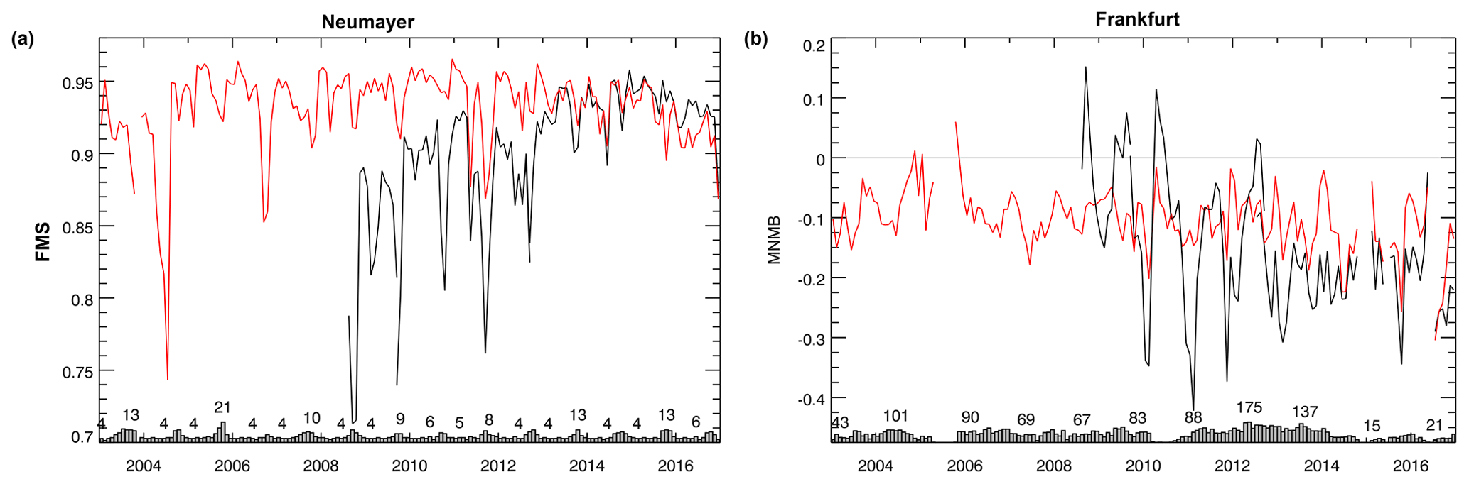
Figure 1Time series from 2003 to 2016 of (a) FMS score of ozone at Neumayer (1000–3 hPa) against ozone-sondes (see Sect. 4.1) and (b) MNMB of CO in the lower troposphere (1000–700 hPa) at Frankfurt am Main airport against IAGOS aircraft data (see Sect. 4.2) from the real-time CAMS system (black) and CAMSRA (red).
Figure 1a shows the “Figure of Merit in space” (FMS; Chang and Hanna, 2004) ozone score at the Antarctic Neumayer Station, and Fig. 1b shows the modified normalised mean bias (MNMB) of CO in the lower troposphere from the CAMS daily forecast system and CAMSRA to illustrate the advantage a reanalysis has over a continuously evolving operational model system. The definitions of the scores are given in the Appendix. The FMS score compares the fit of the model ozone profiles to ozonesonde profiles (here calculated from the surface to 3 hPa), and the score is between 1 (perfect fit) and 0. Figure 1 illustrates the improvements in the near-real-time (NRT) CAMS system with time. In the earlier years the CAMS system did not adequately reproduce the low values and vertical distribution of the Antarctic ozone hole (Flemming et al., 2011; Inness et al., 2013), which is shown by the low FMS scores in austral spring from 2008 to 2012 (Fig. 1a). The CAMSRA has much improved FMS scores during those years and a better consistency in performance between earlier and later years. The time series of MNMB of CO in the lower troposphere (Fig. 1b) also shows problems of the NRT system in the earlier years in the Northern Hemisphere (NH) during winter, when CO values were strongly underestimated (Inness et al., 2013). There is still an underestimation of lower tropospheric CO in the CAMSRA, but the MNMB is now considerably smaller, especially during NH winter, and more constant.
The aim of this paper is to document the new CAMSRA dataset for future reference. The paper gives information about the model and data assimilation setup used to produce CAMSRA, presents initial validation results, and intercompares CAMSRA with CIRA and MACCRA. Additional validation of CAMSRA can be found in reanalysis validation reports (Eskes et al., 2018) and in a validation paper that is in preparation (Wagner et al., 2019).
This paper is structured in the following way. Section 2 describes the CAMS model, the data assimilation system and the emission datasets used to produce the CAMS reanalysis. Section 3 lists the assimilated AC observations and bias correction procedure. Section 4 gives validation results for some of the reactive gases and aerosols, and Sect. 5 presents the conclusions.
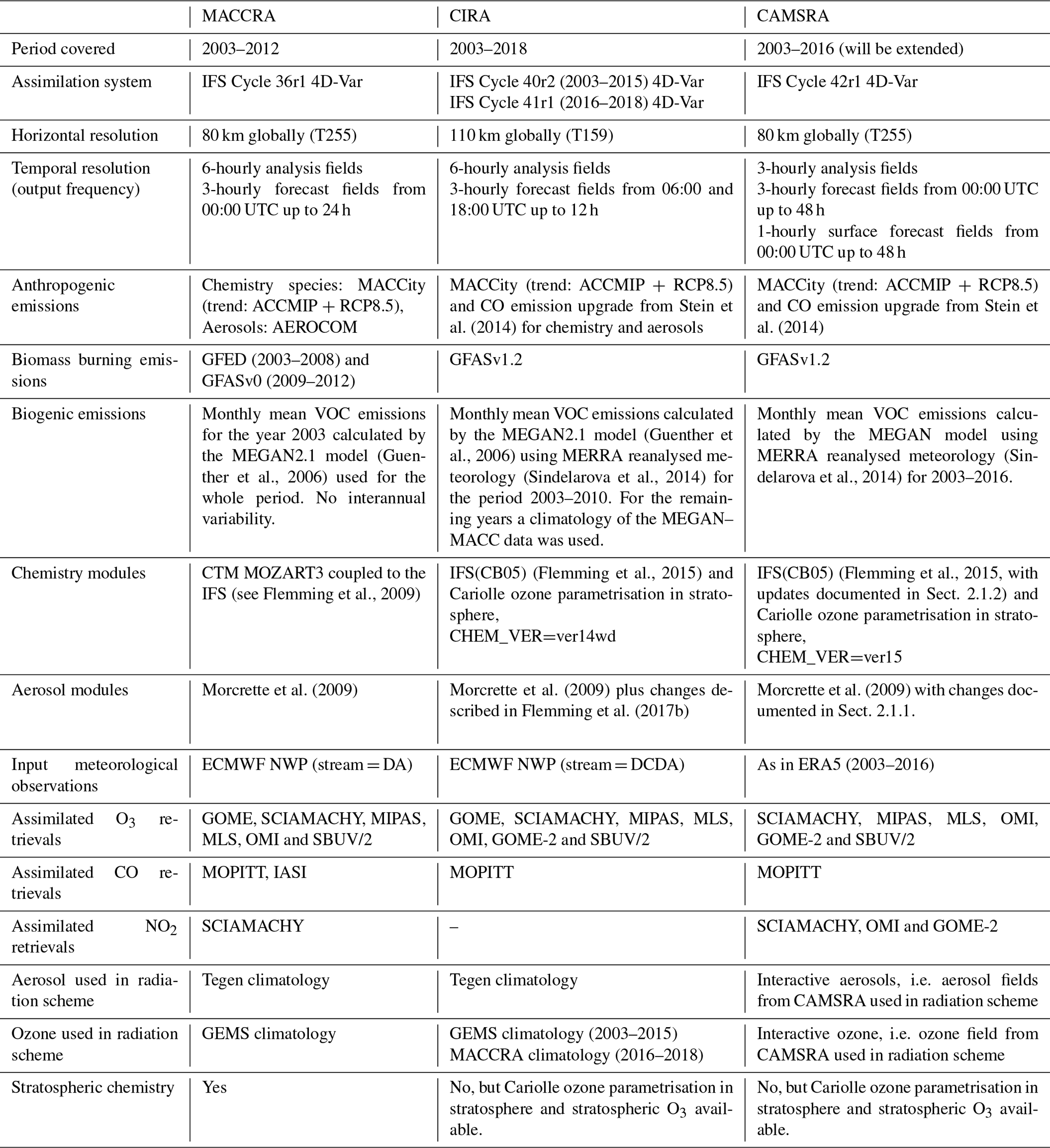
An overview of the main differences and commonalities of the three reanalyses, MACCRA, CIRA and CAMSRA, discussed in this paper is given in Table 1.
Table 1Important commonalities and differences between CAMSRA, CIRA and MACCRA.
2.1 CAMS model system
The IFS aerosol and chemistry modules applied in CAMSRA were similar to those in CIRA, and more details about the modules are given in Flemming et al. (2015) and references therein. Major updates relative to CIRA are described in the Sect. 2.1.1 and 2.1.2 below. The meteorological modelling part of the IFS changed from cycle 40R1 used for CIRA to cycle 42R1 used for CAMSRA (see also Table 1).
2.1.1 Aerosol model updates
The CAMS aerosol model component of the IFS was previously described in Morcrette et al. (2009). It is a hybrid bulk–bin scheme with 12 prognostic tracers, consisting of three bins for sea salt depending on size (0.03–0.5, 0.5–5 and 5–20 µm), three bins for dust (0.030–0.55, 0.55–0.9 and 0.9–20 µm), hydrophilic and hydrophobic organic matter (OM), and black carbon (BC), plus sulfate aerosol and a gas-phase sulfur dioxide (SO2) precursor. The different aerosol types are treated as externally mixed, i.e. separate particles. Transport by advection, convection and diffusion is handled by the meteorological model component of the IFS. The aerosol scheme includes prescribed and online emissions (as described in Sect. 2.2), dry and wet deposition, production of sulfate from SO2, and ageing of hydrophobic OM and BC to hydrophilic OM and BC. Nitrate aerosols are not yet included in the aerosol scheme. The missing nitrate aerosol is likely to cause an underestimation of total aerosol in the forecast model in regions where nitrate would be a significant component. The total aerosol will be corrected by the assimilation of total AOD observations.
The aerosol model used in the CAMS reanalysis contains these updates relative to CIRA:
-
Aerosol optical properties were updated, especially for organic matter (as described in Bozzo et al., 2017).
-
Bug fixes were applied to sedimentation, which was unreasonably weak for some dust and sea-salt bins, with corresponding retuning of sea-salt scavenging.
-
SO2 dry deposition velocities were updated to use monthly values computed by Météo-France's Surface Module of the MOCAGE model (SUMO; Michou et al., 2004). They now match those used in the chemistry scheme.
-
A new parameterisation of anthropogenic secondary organic aerosol (SOA) production was implemented, proportional to MACCity CO emissions, as suggested in Spracklen et al. (2011).
-
There was a more detailed SO2 to sulfate aerosol conversion with dependence on temperature and relative humidity, and there was an overall decrease in the conversion timescale, especially at high latitudes.
-
The sulfate dry deposition velocity was increased over the ocean.
-
A proportional mass fixer used for chemistry (Diamantakis and Flemming, 2014) was extended to aerosol species.
-
In CIRA, emissions from the Global Fire Assimilation System (GFAS) of black carbon (BC) were scaled by a globally constant factor of 3.4, which had been derived by comparing BC from a 6-month assimilation run with a forecast only run. In CAMSRA the same approach was used but comparing 12 years of CIRA data against a control run without data assimilation. This made it possible to derive a geographically varying (but temporally constant) scaling factor for BC GFAS emissions in CAMSRA.
-
The SO2 emissions in CAMSRA were separated between low-level (20 % of total emissions, which are emitted as part of the diffusion scheme) and high-level emissions (80 % of total emissions which are released in the two lowest model levels). In CIRA all SO2 emissions were released at the surface as part of the diffusion scheme.
2.1.2 Chemistry module updates
The chemical mechanism of the IFS is a modified and extended version of the CB05 (Yarwood et al., 2005) chemical mechanism for the troposphere, as implemented in the CTM TM5 (Huijnen et al., 2010). CB05 describes tropospheric chemistry with 55 species and 126 reactions. Stratospheric ozone chemistry in IFS(CB05) is parameterised by a “Cariolle-scheme” (Cariolle and Déqué, 1986; Cariolle and Teyssèdre, 2007). Wet deposition is modelled following Jacob (2000), and monthly mean gridded dry deposition velocities calculated by the SUMO model of Météo-France (Michou et al., 2004) were used to calculate dry deposition. The chemistry module of the IFS is documented in more detail in Flemming et al. (2015) and Flemming et al. (2017b). The following updates of the chemistry scheme from the configuration used in CIRA were applied to produce CAMSRA:
-
update of heterogeneous rate coefficients for N2O5 and HO2 based on prognostic clouds and aerosol,
-
modification of photolysis rates by prognostic aerosol,
-
dynamic tropopause definition based on the temperature profile for coupling to the Cariolle scheme in the stratosphere and for tropospheric mass diagnostics,
-
bug fixes, in particular for the diurnal cycle of dry deposition whose correction has decreased the ozone dry deposition flux by about 15 %–20 %.
It should be noted that the schemes for aerosol and chemistry in IFS(CB05) are largely independent, which means, in particular, that both the aerosol and the chemistry scheme carry their own SO2 variable. The conversion of the aerosol SO2 to sulfate aerosol is modelled in the aerosol scheme by prescribed conversion rates (Morcrette et al., 2009), whereas SO2 in the chemistry scheme is subject to gas-phase and aqueous-phase chemistry. The sulfate of the chemistry scheme neither contributes to the aerosol optical properties nor is it corrected by data assimilation. However, the first steps to link chemistry and aerosol schemes have been undertaken, and the aerosol model affects the chemical composition by using the aerosol surface area density in the heterogenous reaction rates of dinitrogen pentoxide (N2O5) and hydroperoxyl (HO2; Huijnen et al., 2014) as well as by using aerosol optical properties for the modification of photolysis rates.
A major difference between the production of CIRA and CAMSRA is that the prognostic ozone and aerosol fields have been used interactively in the NWP radiation scheme in CAMSRA. For CIRA climatologies of ozone derived from MACCRA (Bozzo et al., 2017) and the Tegen et al. (1997) aerosol climatology were used in the radiation scheme. The evaluation of the meteorological parameters is beyond the scope of this paper. Nevertheless, little differences were found by introducing prognostic ozone and aerosol because the meteorological analysis is well constrained by the assimilated observations. Furthermore, no change in the evaluation of the AC parameters could be identified when using ozone and aerosol interactively in the radiation scheme.
2.2 Emissions
Great care has been taken to ensure that the emission datasets are consistent in time and that consistent anthropogenic, biogenic and biomass burning emissions were used for the aerosol and chemistry fields. The emission datasets are listed in Table 1. The emissions are injected at the surface and distributed over the boundary layer by the model's convection and vertical diffusion scheme. The only exception is the aerosol SO2 emissions, of which 20 % are emitted at the surface as part of the diffusion scheme and 80 % are emitted in the two lowest model levels (see Sect. 2.1.1). The emissions datasets used in CAMSRA include emissions from anthropogenic, biogenic, natural and biomass burning sources.

Figure 2Monthly CO emissions in Tg yr−1 from anthropogenic sources (MACCity with correction from Stein et al., 2014) for (a) the globe, (b) East Asia, (c) Europe and (d) North America for the period 2003–2016.
Anthropogenic emissions were from the MACCity inventory (Granier et al., 2011), with modifications to increase wintertime road traffic emissions over North America and Europe following the correction of Stein et al. (2014). These emissions were also used in CIRA, while they were used without the Stein et al. (2014) correction in MACCRA. The MACCity inventory covers the period 1960–2010 and is updated for subsequent years using the representative concentration pathway (RCP) version 8.5. The RCP 8.5 (business as usual) scenario was chosen, as it includes information on regional emissions after 2000 (Van Vuuren et al., 2010; Riahi et al., 2011). The anthropogenic MACCity emissions for CO are shown in Fig. 2, and the emissions for NO are shown in Fig. 3. The CO emissions decrease over Europe and North America in the range of 1 % to 5 % per year but increase over Southeast Asia by a similar amount. The global trend for CO is close to zero. The MACCity NO emissions decrease with time over Europe and North America but increase over East Asia until 2015, which is in contrast to satellite-derived emission inventories that show a peak over China in 2012 (e.g. Ding et al., 2017). Anthropogenic emissions of black carbon, organic carbon and SO2 were also taken from MACCity. Emissions of anthropogenic SOA were estimated by applying a scaling factor of 0.2 to the MACCity (i.e. non-biomass burning) CO emissions, as suggested in Spracklen et al. (2011).
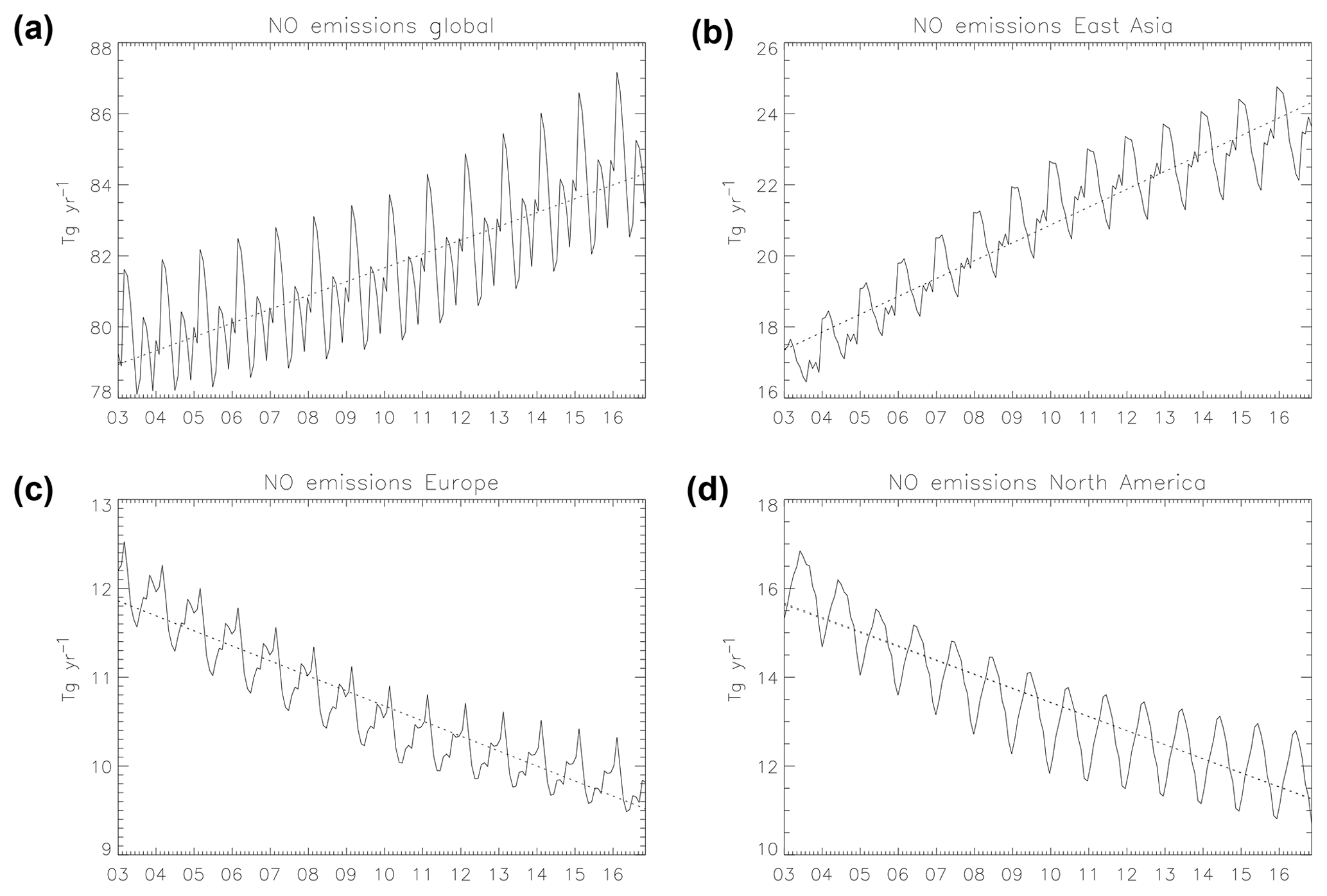
Figure 3Monthly NO emissions in Tg yr−1 from anthropogenic sources (MACCity) for (a) the globe, (b) East Asia, (c) Europe and (d) North America for the period 2003–2016.
Monthly mean biogenic emissions of the chemical species were calculated offline by the MEGAN2.1 model (Guenther et al., 2006) that used meteorological fields from the MERRA-2 reanalysis following Sindelarova et al. (2014) for the full period of CAMSRA. Natural emissions from soils and oceans for NO2, dimethyl sulfate (DMS) and SO2 were taken from the Precursors of ozone and their effects in the Troposphere (POET) database for 2000 (Granier et al., 2005; Olivier et al., 2003).
Daily global biomass burning emissions of reactive gases and aerosols were provided by the Global Fire Assimilation System, version 1.2 (GFASv1.2), based on satellite retrievals of fire radiative power (Kaiser et al., 2012). The archive of GFASv1.2 data covers the period 2003–present and was also used in CIRA. In MACCRA early versions of the Global Fire Emissions Database (GFEDv3.1; van der Werf et al., 2010) were used from 2003 to the end of 2008, and daily GFASv1.0 data were used from 2009 to 2012. GFEDv3.1 is on average 20 % lower than GFASv1.2 (Inness et al., 2013). Figure 4 shows the GFASv1.2 time series of monthly mean total carbon wildfire emissions for each of the main continental regions, excluding Antarctica, between 2003 and 2016. The emissions from GFEDv3.1 and GFASv1.0 are also shown for comparison. The CO biomass burning emissions do not show a significant trend but considerable inter-annual variability. Africa is usually the largest source of CO biomass burning emissions, but under El Niño conditions Asian emissions (and in particular emissions from maritime Southeast Asia) reach similar values. Most notable here are the Asian emissions during the Indonesian fires in September and October 2015 that caused by far the highest annual wildfire emissions as well as the highest total monthly CO emissions in the whole period covered by GFAS (Huijnen et al., 2016).
The aerosol model has additional online parameterisations to calculate sea salt (Monahan et al., 1986) and dust surface fluxes based on surface winds and other factors (Ginoux et al., 2001).
2.3 CAMS data assimilation system
The IFS uses an incremental 4D-Var data assimilation system (Courtier et al., 1994) for the CAMS reanalysis, with 12 h assimilation windows from 09:00 to 21:00 and 21:00 to 09:00 UTC and two minimisations at spectral truncations T95 (∼210 km) and T159 (∼110 km). In the CAMS 4D-Var a cost function that measures the differences between the model's background fields and the observations is minimised in order to obtain the best possible forecast through the length of the assimilation window by adjusting the initial conditions. Several atmospheric composition fields (i.e. O3, CO, NO2 and total aerosol mass mixing ratio) are included in the control vector and minimised together with the meteorological control variables. The background errors for the atmospheric composition fields were either calculated with the National Meteorological Center (NMC) method (Parrish and Derber, 1992) or from an ensemble of forecast differences (Inness et al., 2015). Both methods allow us to calculate differences between pairs of background fields which have the statistical characteristics of the background errors. The background errors for the chemical species are univariate, i.e. the error covariance matrix between chemical species or between chemical species and dynamical fields is diagonal. Hence each species is assimilated independently from the others. More information about the data assimilation system and background errors for the chemical fields can be found in Inness et al. (2015). The aerosol assimilation is described in Benedetti et al. (2009), and the background errors used for the aerosol assimilation are described in Benedetti and Fisher (2007).
The aerosol assimilation is less constrained than the assimilation of the chemical species because the model has 12 different aerosol components (see Sect. 2.1.1), while the assimilated observations are retrievals of total AOD. Therefore, the total aerosol mass mixing ratio, defined as the sum of the aerosol species, is used as control variable, and the analysis increments are repartitioned into the individual aerosol components (the SO2 precursor is excluded from this process, as it is not visible in the AOD observations) according to their fractional contribution to the total aerosol mass (Benedetti et al., 2009). Flemming et al. (2017b) have shown that this can lead to problems, as the relative fraction of the aerosol components is not conserved during the whole assimilation procedure because of differences in aerosol lifetime associated with differences in their removal processes. Aerosol components with a longer atmospheric lifetime can retain the change imposed by the increments for longer and may thereby change the relative contributions. Also, if the underlying aerosol model has a bias in one aerosol species, e.g. it overestimates the species and thereby contributes a bigger fraction to the total aerosol mass mixing ratio than it should, the assimilation can exacerbate this by attributing a greater proportion of the increment to this species and enhancing the bias even further. This was the case in CIRA, where it led to an unrealistic overestimation of sulfates (Flemming et al., 2017b). Sulphates are reduced in CAMSRA (see Fig. 20 below).
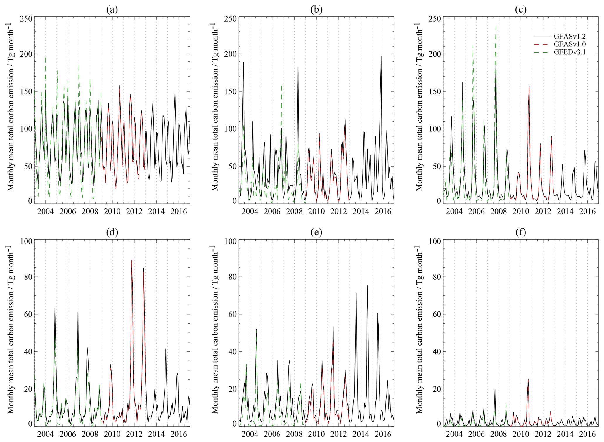
Figure 4Time series of monthly total carbon wildfire emissions in Tg month−1 from GFASv1.2 (2003–2016, black solid line), GFASv1.0 (2009–2012, red dashed line) and GFEDv3.1 (2003–2008, green dashed line) for geographical domains covering (a) Africa, (b) Asia, (c) South America, (d) Australia, (e) North America and (f) Europe.
2.4 CAMSRA data product
The spatial resolution of the CAMS reanalysis is a reduced Gaussian grid at a spectral truncation of T255, which is equivalent to grid spacing of approximately 80 km globally ( grid). The vertical model resolution consists of 60 hybrid sigma–pressure (model) levels with a model top at 0.1 hPa. The data are available as 3-hourly analyses and 48 h forecasts, initialised daily from analyses at 00:00 UTC. Three-dimensional model-level forecast fields are available every 3 h from forecast hour 0 to 48, and surface forecast fields are available at hourly intervals. Monthly mean fields are also provided. Atmospheric data are archived on 60 model levels and are also interpolated to 25 pressure levels, 10 potential temperature levels, and 1 potential vorticity level. Surface and total column diagnostics are also available (https://software.ecmwf.int/wiki/display/CKB/CAMS +Reanalysis+data+documentation#CAMSReanalysisdata documentation-Parameterlistings, last access: 15 March 2019). An inventory of the available model fields can be found at http://apps.ecmwf.int/data-catalogues/cams-reanalysis/?class=mc&expver=eac4, (last access: 15 March 2019), and more information can be found at https://atmosphere.copernicus.eu (last access: 15 March 2019). The data will become available from the Copernicus Atmosphere Data Store.

Figure 5AC data assimilated in the CAMS reanalysis between 2003 and 2016. In red retrievals are shown for which no averaging kernels were used; in green those where averaging kernels were used are shown.
3.1 Observations
The atmospheric composition satellite retrievals of O3, CO, NO2 and AOD that were assimilated to produce CAMSRA are shown in Fig. 5 and listed in Table 2. The table also shows the blacklist criteria applied to the data, i.e. the criteria that determine when data were not used.
Table 2Satellite retrievals of atmospheric composition that were assimilated in the CAMS reanalysis. TC is total column, TRC is tropospheric column, PROF is profiles, PC is partial columns, QR is quality flag given by data providers, SOE is solar elevation, MODORO is model orography, PRESS_RL is pressure at bottom of layer, LAT is latitude and SAA is area of the South Atlantic Anomaly.
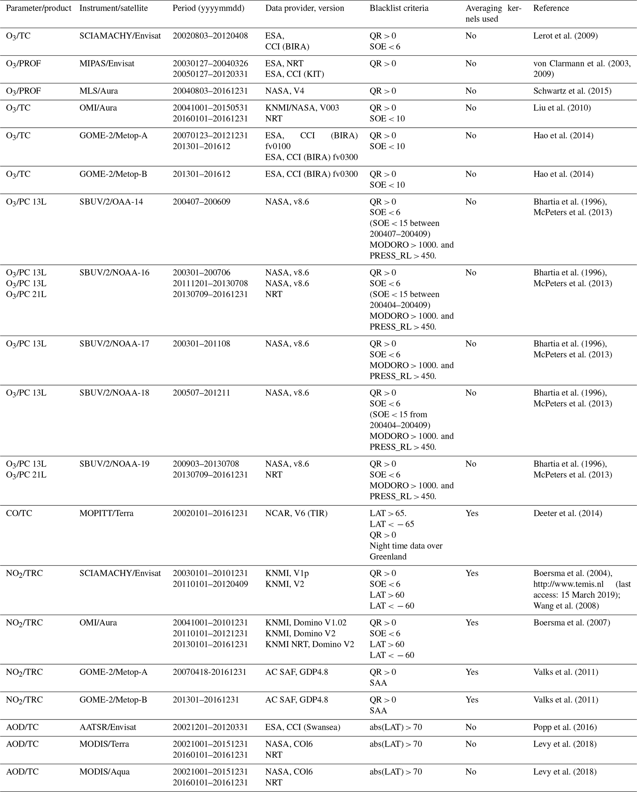
Retrievals from a range of instruments were used for O3. These included total column O3 (TCO3) retrievals from the SCanning Imaging Absorption SpectroMeter for Atmospheric CHartographY (SCIAMACHY) instrument, the Ozone Monitoring Instrument (OMI) and the Global Ozone Monitoring Experiment-2 (GOME-2), O3 profile data from the Michelson Interferometer for Passive Atmospheric Sounding (MIPAS) and Microwave Limb Sounder (MLS; used down to 215 hPa), and O3 partial columns from the Solar Backscatter Ultraviolet (SBUV/2) radiometer. For SBUV/2 the version 8.6 data record (McPeters et al., 2013) was used until July 2013 and NRT version 8 data afterwards. The version 8.6 data are available at 21 vertical layers but were converted into a 13-layer product by CAMS to reduce smoothing errors by combining the layers between 16 hPa and the surface. The NRT SBUV/2 data were the same data used in the CAMS real-time analysis and used at the 21 L resolution. Changing the NRT data was necessary, as the reprocessed data were not available after July 2013. We do not notice a change in the ozone analysis field at this time because the analysis is well constrained by the other assimilated O3 data, in particular by the MLS profiles.
For CO, Measurement of Pollution in the Troposphere (MOPITT) thermal infrared (TIR) Version 6 total column CO (TCCO) retrievals were assimilated in CAMSRA. These retrievals are most sensitive to CO in the mid-troposphere and upper troposphere (Deeter et al., 2013) and are retrieved from the TIR band near 4.7 µm. The main improvements compared with the older MOPITT versions used in CIRA (MOPITT V5) and MACC (MOPITT V4) are a correction of a bias in geolocation, improved meteorological data based on the MERRA reanalysis and updated CO a priori profiles (Deeter et al., 2014). In contrast to MACCRA no IASI CO retrievals (George et al., 2009; Clerbaux et al., 2009) were assimilated in CAMSRA because using them led to a discontinuity in MACCRA (Inness et al., 2013; Flemming et al., 2017b).
For NO2, tropospheric column retrievals from SCIAMACHY, OMI and GOME-2 were assimilated in CAMSRA. This is an improvement over CIRA (where no NO2 data were assimilated) and MACCRA (where only SCIAMACHY NO2 data were assimilated). Where possible, new reprocessed datasets were used in CAMSRA. However, due to time constraints it was not possible to acquire and process new observations for all the instruments, and for NO2 from SCIAMACHY and OMI, the data that were already available had to be used. The SCIAMACHY NO2 retrievals used in CAMSRA were the same data version assimilated in MACCRA (Koninklijk Nederlands Meteorologisch Instituut – KNMI; V1p from 2003 to 2011, V2 2011–April 2012). The OMI NO2 data were also produced by KNMI (Boersma et al., 2007, 2011) and consisted of offline DOMINO (version 1.0.2) data from October 2004 to 2010, the offline DOMINO (version 2) retrieval for 2011–2012 and NRT DOMINO retrievals (version 2) from 2013 onwards. The GOME-2 data were the offline GDP4.8 data produced by the EUMETSAT Satellite Application Facility for Atmospheric Composition Monitoring/Deutsches Zentrum für Luft- und Raumfahrt (ACSAF/DLR; Valks et al., 2011) until the end of 2016. GOME-2 NO2 retrievals from Metop-A were assimilated from April 2007 onwards, and retrievals from Metop-B were assimilated from January 2013. In previous studies (Inness et al., 2015) the impact of the assimilation was shown to be small for short-lived species like NO2 because at least some of the changes applied to the initial conditions by the analysis were frequently insignificant compared with the prevalent emissions of nitrogen oxides () and were lost again in the subsequent forecasts. By assimilating NO2 retrievals from satellites with different overpass times (09:30 local time – LT – for GOME-2, 10:00 LT for SCIAMACHY, 13:30 LT for OMI) the impact of the assimilation is expected to be increased, and the diurnal cycle of NO2 is expected to be better represented. The discontinuity in the assimilated NO2 products could influence the long-term ozone analysis. Unfortunately, as there is no additional experiment where O3 data but no NO2 data were assimilated, it is not possible to infer this information from the CAMS reanalysis. We have seen in the past (Inness et al., 2015) that the impact of the NO2 assimilation is generally small, so we do not expect this to lead to problems in the ozone analysis.
For aerosols, Collection 6 retrievals of total AOD at 550 nm from the Moderate Resolution Imaging Spectroradiometer (MODIS; Levy et al., 2018) aboard the Aqua and Terra satellites that were produced with the enhanced Deep Blue (DB) and Dark Target (DT) algorithms over land and a DT over-water algorithm over the ocean were used in CAMSRA. The main scientific improvement in the algorithm of Collection 6, compared with the Collection 5 observations used in MACCRA and CIRA, is the introduction of a wind speed dependence over the oceans. This addressed the known bias in Collection 5 over midlatitude oceans, particularly in the Southern Hemisphere (SH). Various minor changes to the processing were also made in Collection 6 for maintenance, giving modest improvements (Levy et al., 2013). The data preparation stage for the MODIS observations prioritises Dark Target and will only use Deep Blue data if no Dark Target observations are available. In addition to MODIS, CAMSRA used retrievals from the Advanced Along-Track Scanning Radiometer (AATSR; Popp et al., 2016) aboard Envisat from 2003 to March 2012. The AATSR and MODIS AOD observations may potentially be coincident, but this is dealt with by the data assimilation system. Solving the cost function balances mismatches for both the model and all observations, taking into account both model and individual observation errors.
Averaging kernels were used in the observation operator for the calculation of the model's first-guess fields for CO and NO2 retrievals as described in Inness et al. (2013).
3.2 Bias correction
A variational bias correction (VarBC) scheme (Dee and Uppala, 2009) where biases are estimated during the analysis by including bias parameters in the control vector was used for several of the AC datasets. In this scheme, the bias corrections are continuously adjusted to optimise the consistency with all information used in the analysis. VarBC was applied to the TCO3 retrievals from OMI, SCIAMACHY and GOME-2, with a global constant and solar elevation as predictors, while the partial column SBUV/2 and profile MLS and MIPAS data were used to anchor the bias correction, i.e. were assimilated without correction. Experience from MACCRA had shown that it was important to have an anchor for the O3 bias correction to avoid drifts in the fields (Inness et al., 2013). The SBUV/2 data were chosen as an anchor because they are a high-quality reprocessed dataset that covers the whole period of CAMSRA. The MLS and MIPAS profile data were not bias corrected because experience in MACCRA had shown that the SBUV/2 data could not anchor all the layers of the higher resolved profile data and that drifts in individual layers could lead to problems in the vertical O3 distribution (Inness et al., 2013). Variational bias correction was also applied to OMI NO2 retrievals, again with a global constant and solar elevation as predictors, while SCIAMACHY and GOME-2 NO2 retrievals were used to anchor the bias correction for NO2. This choice was made because SCIAMACHY and GOME-2 generally agree better with the CAMS NO2 fields, while OMI has a larger bias (see Figs. S5 and S6 in the Supplement) and also suffers from a row anomaly (see Supplement) that reduces the number of good data with time. A validation of the diurnal cycle of NO2 is needed in the future to assess if using GOME-2 as anchor and applying bias correction to OMI could introduce spurious biases into the OMI NO2 data, leading to inaccurate diurnal NO2 variations in the model. However, as the NO2 bias correction is part of the control vector and is continuously adjusted to optimise the consistency with all parameters used in the analysis, and as the assimilation of NO2 usually only has a small impact in the CAMS system because of its short lifetime (Inness et al., 2015), we do not expect this to be a problem. Hopefully a validation of the diurnal cycle of NO2 will be included in the validation paper that is under preparation. For CO, no bias correction was applied in CAMSRA because data from only one instrument were assimilated, and it was not possible to anchor the VarBC. For AOD, experience had shown that it was not necessary to anchor the bias correction for the aerosol data, and VarBC was applied to both MODIS retrievals and to AATSR. The predictors for AOD were a global constant and the 2 m wind speed over sea.
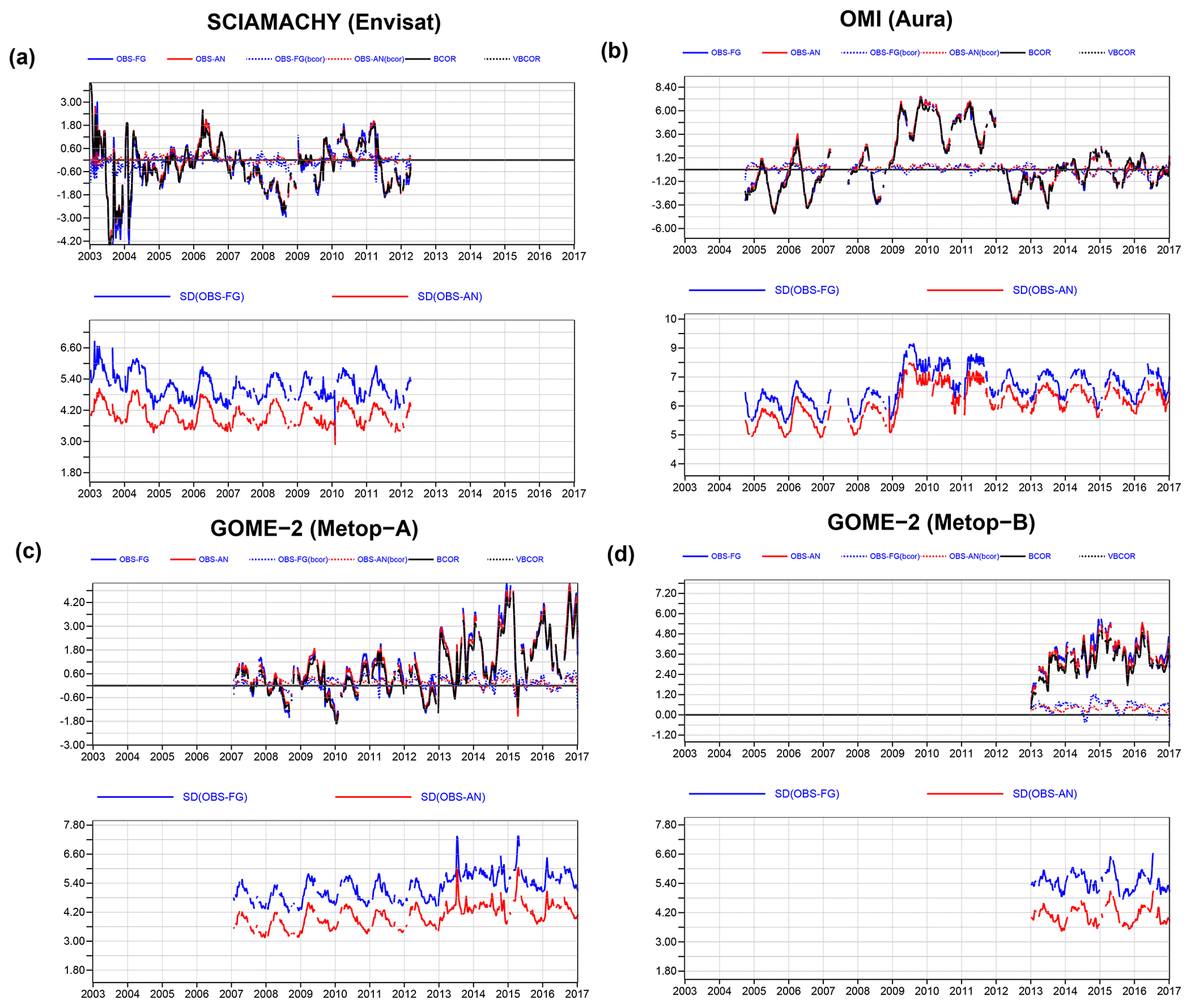
Figure 6Time series of global mean monthly mean TCO3 departures (top plots) and standard deviations of departures (bottom plots) of (a) SCIMACHY, (b) OMI, (c) GOME-2A and (d) GOME-2B. The red lines show analysis departures, the blue lines first-guess departures, black lines bias correction, and dotted red and blue lines the bias corrected analysis and first-guess departures. Values are in DU. More information about departures can be found in the Supplement.
The bias correction helps to ensure good time consistency when blending various datasets and adapts to changing biases of the data. An example is shown in Fig. 6, which shows time series of monthly mean analysis departures (i.e. observations minus analysis fields) and first-guess departures (i.e. observations minus model first guess) for the four TCO3 retrievals (SCIAMACHY, OMI, GOME-2A and GOME-2B) as well as for the applied bias correction. For all four TCO3 datasets the analysis draws to the observations, and the standard deviations of the analysis departures are reduced compared to those of the first-guess departures. The plots show that the bias correction (black lines) is different for all instruments, successfully adapts to changes in the data, and removes the biases between total column data and the model. OMI data (Fig. 6b) between 2009 and 2011, for example, show different behaviour than during the rest of the time series, with larger departures (due to larger observation values, not shown) and the need for larger bias correction. However, the bias correction successfully accounts for this, and the bias corrected departures are small and stable. The reason for this change is a deterioration in the OMI row anomalies (Torres et al., 2018, see their Fig. 1; Schenkeveld et al., 2017). More information about this can be found in the Supplement. Thanks to the bias correction removing such biases, the bias corrected departures (dotted lines) are small and stable for all four instruments.
Monitoring time series for all the atmospheric composition datasets assimilated in CAMSRA are shown in the Supplement. One important feature to note from the Supplement is that SCIAMACHY NO2 (Fig. S5) has much larger positive departures during 2003 than during the rest of the period. This affects the quality of the NO2 analysis during 2003 (see Fig. 18 in Sect. 4.3 below).
In this section, analysis fields for O3, CO, NO2 and AOD from CAMSRA are compared to fields from CIRA and MACCRA to highlight some of the improvements in CAMSRA and to point out some of the problems potential users should be aware of. We concentrate on these four species because they were the ones assimilated in CAMSRA and validation data are available. There are, of course, a lot more species available from CAMSRA that are not covered in this paper. A more thorough validation of the CAMS reanalysis is beyond the scope of this paper and given in validation reports available from the CAMS website (Eskes et al., 2018; available at https://atmosphere.copernicus.eu/sites/default/files/2018-09/CAMS84_2015SC2_D84.7.1.4_Y14_v1.pdf, last access: 15 March 2019).
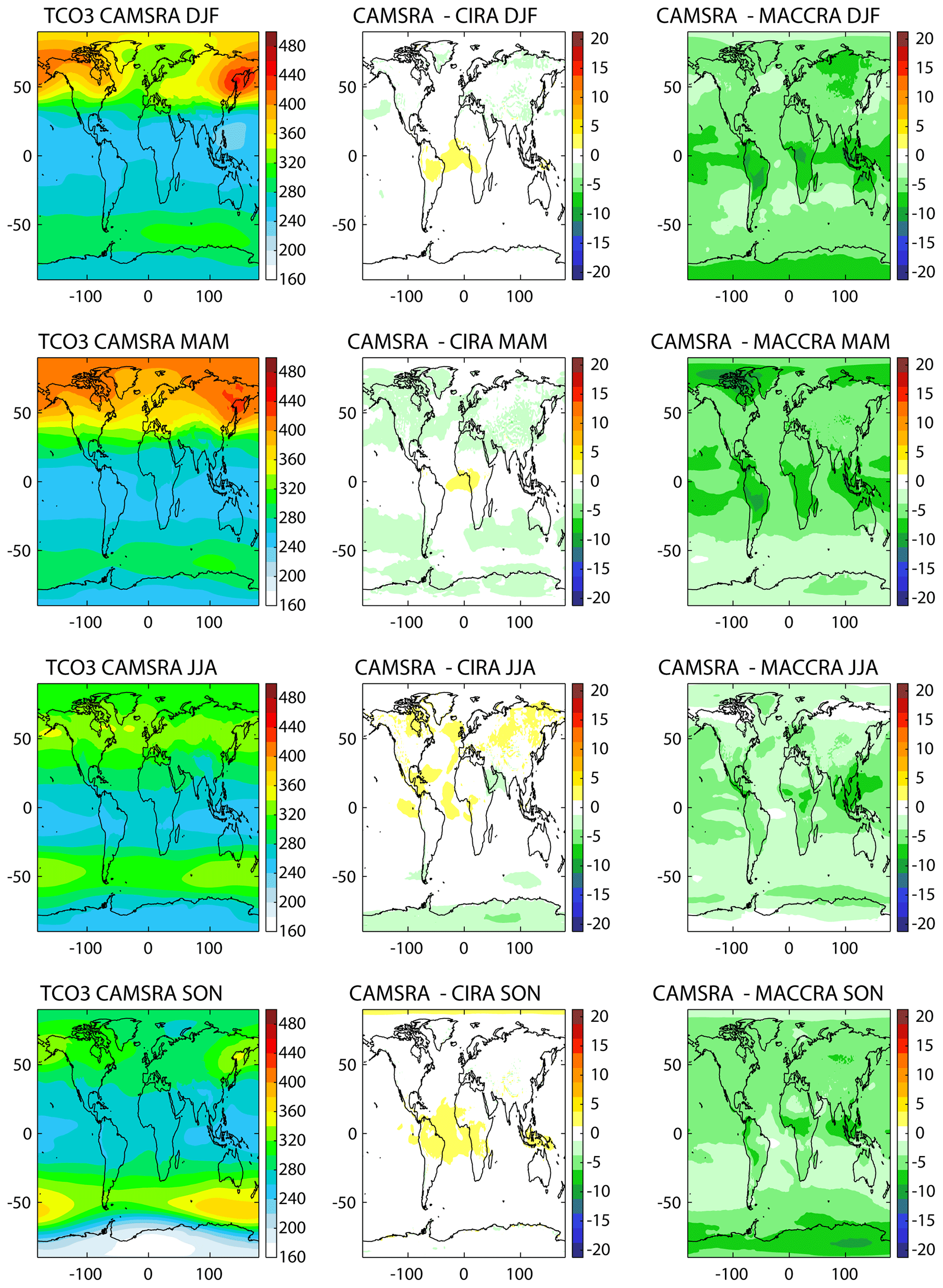
Figure 7Seasonally averaged TCO3 from CAMSRA (2003–2016, left), difference between CAMSRA and CIRA (middle), and difference between CAMSRA and MACCRA (right, 2003–2012 only) in DU for the seasons DJF (row 1), MAM (row 2), JJA (row 3) and SON (row 4).
4.1 Ozone
We start by looking at TCO3, which is dominated by stratospheric O3, and then look at tropospheric and surface O3, which are more relevant for air quality users. Figure 7 shows the seasonally averaged TCO3 from CAMSRA and the differences between this dataset and CIRA and MACCRA. The TCO3 differences between CAMSRA and CIRA are very small (below 2DU, <1 %), with slightly larger differences (5 DU, < 3 %) in June, July and August (JJA) over Antarctica. CAMSRA TCO3 is slightly higher than CIRA over the Tropical Atlantic in all seasons and in NH midlatitudes in JJA; it is lower over NH midlatitudes during December, January and February (DJF) and March, April and May (MAM); and it is lower over SH midlatitudes in MAM and JJA. The differences between CAMSRA and MACCRA are larger, with CAMSRA lower than MACCRA everywhere (up to −10 DU, < 5 %).
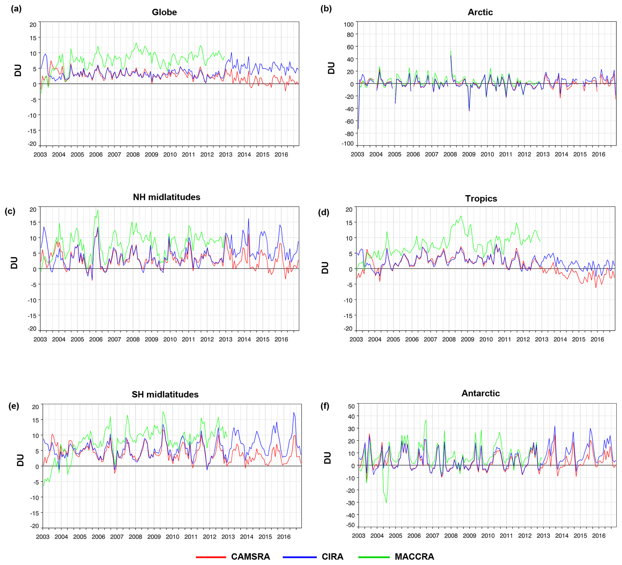
Figure 8Time series of monthly mean TCO3 bias in DU from the three reanalyses compared to WOUDC Dobson data for the areas (a) globe, (b) Arctic, (c) NH midlatitude, (d) tropics, (e) SH and (f) Antarctic. About 50–60 stations were available from 2003 to 2014, dropping to about 40 stations after 2014. CAMSRA is shown in red, CIRA in blue and MACCRA in green.
Table 3Mean biases and standard deviations from MACCRA, CIRA and CAMSRA relative to WOUDC Dobson data (shown in Fig. 8) in DU. The values are calculated for the period 2003–2012, and the values in brackets are calculated for CIRA and CAMSRA for the period 2003–2016. Numbers in italics mark where MACCRA or CIRA have larger biases or standard deviation than CAMSRA, and numbers in bold mark where their values are smaller.
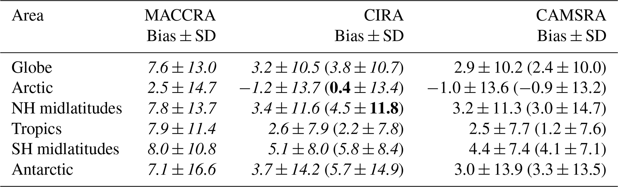
To assess if the differences seen between CAMSRA and the older reanalyses are an improvement we compare TCO3 from the reanalyses to independent, i.e. not used in the analysis, Dobson sun photometer measurements (Fig. 8) obtained from the World Ozone and Ultraviolet Radiation Data Centre (WOUDC). The Dobson data are well calibrated, with a precision of 1 % (Basher, 1982). The mean biases and their standard deviations for the three reanalyses against the Dobson data are given in Table 3. Figure 8 shows that MACCRA has the largest (positive) biases relative to these data and that CAMSRA agrees better with the independent observations in all areas. CAMSRA has smaller biases than the other two reanalyses in all areas, except in the tropics after 2013, when CIRA has a smaller bias. CAMSRA and CIRA are very close from 2003 to 2012 but diverge more from 2013 onwards, when the version of the MLS profiles used in CIRA changed from version 2 to NRT version 3.4 (Flemming et al., 2017b). In these later years, CAMSRA is generally better than CIRA, except in the tropics. The largest biases for CAMSRA (up to 25 DU) are found over Antarctica during the ozone hole season after 2013. Figure 8 shows that there is no noticeable impact during 2009–2011 when degraded OMI observations were assimilated (Fig. 6), illustrating the success of the variational bias correction (Sect. 3) for the TCO3 data. Table 3 confirms that CAMSRA has the smallest mean biases of the three reanalyses when averaged over the period 2003–2012 and also has smaller biases than CIRA for the period 2003–2016 in all areas except the Arctic. The average global mean biases for the period 2003–2012 are 2.9±10.2 DU for CAMSRA, 3.2±10.5 DU for CIRA and 7.6±13.0 DU for MACCRA. The biases for the other areas can be found in Table 3. We see that for TCO3, CAMSRA is clearly a better product than the older reanalyses.
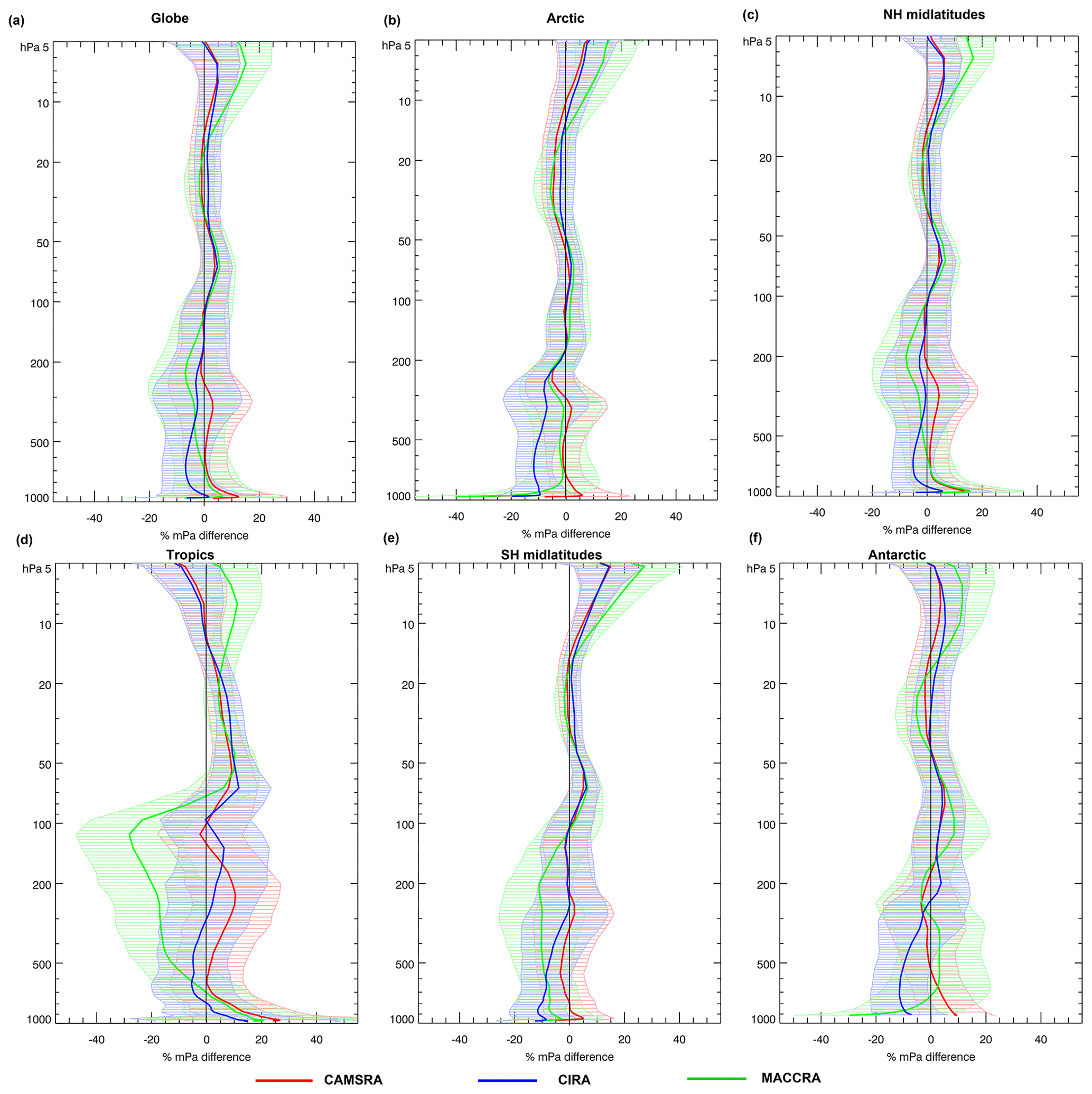
Figure 9Mean relative O3 bias in % between CAMSRA (red), CIRA (blue), MACCRA (green) and ozone-sondes averaged over (a) the globe, (b) Arctic, (c) NH midlatitudes, (d) tropics, (e) SH midlatitudes and (f) Antarctic. The shaded areas show plus or minus 1 standard deviation. For CAMSRA and CIRA the average is calculated over the period 2003–2016, and for MACCRA the average is calculated only for 2003–2012.
While it is relatively easy to reproduce a good TCO3 field by assimilating TCO3 data, reproducing the vertical structure of the O3 field is more difficult, and the CAMS system had problems with this in the past (Flemming et al., 2011). We therefore also carry out a comparison against independent ozone-sondes to evaluate the vertical structure of model biases in the troposphere and stratosphere. The ozone-sonde data used for the validation were acquired from a variety of data centres: WOUDC, Southern Hemisphere Additional Ozonesondes (SHADOZ), Network for the Detection of Atmospheric Composition Change (NDACC) and campaigns for the Determination of Stratospheric Polar Ozone Losses (MATCH). The precision of electrochemical concentration cell (ECC) ozone-sondes is on the order of ±5 % in the range between 200 and 10 hPa, between −14 % and +6 % above 10 hPa, and between −7 % and +17 % below 200 hPa (Komhyr et al., 1995). Larger errors are found in the presence of steep gradients and where the ozone amount is low. The same order of precision was found by Steinbrecht et al. (1998) for Brewer–Mast sondes. Mean relative difference between the three reanalyses and ozone-sondes and the standard deviations of the biases are shown in Fig. 9 for the globe, Arctic, NH midlatitudes, tropics, SH midlatitudes and Antarctic. For MACCRA the average is only for the period 2003–2012. In general, CAMSRA agrees to within 10 % with the sondes. The best agreement between the reanalyses and the sondes is found in the stratosphere, where the assimilated O3 data constrain the analyses well. Differences between the reanalyses are larger in the troposphere, where the impact of the assimilation is smaller (Inness et al., 2015) and differences in the chemistry schemes, emissions and transport become more important. CAMSRA and CIRA agree well above about 200–100 hPa, while MACCRA overestimates O3 in all areas above about 15 hPa. While this overestimation of upper stratospheric and mesospheric O3 in MACCRA will not affect the TCO3 bias, ozone in this region is important for radiative transfer and the associated heating rates. A smaller bias in this region will make CAMSRA a better dataset to be used as climatology in, for example, radiation schemes or radiance observation operators. CAMSRA has larger O3 values than CIRA in the troposphere which leads to an increased bias with respect to the sondes in the tropics but smaller biases in the other areas. Near the surface, CAMSRA has a positive bias. The largest differences between the reanalyses in the troposphere are found in the tropics. Here MACCRA underestimates O3 in the mid-troposphere and upper troposphere, with mean biases of up to −30 %, but absolute differences are small because O3 values in the tropical upper troposphere and lower stratosphere are low. MACCRA also has a large negative bias near the surface in the Arctic and Antarctic. Here, improvements to the background error statistics (Inness et al., 2015), in particular to the vertical correlations of the background errors, led to big improvements in CIRA and CAMSRA compared with MACCRA.

Figure 10Time series of the modified normalised mean bias (MNMB) in the free troposphere (750–300 hPa) of the reanalyses versus ozone-sondes for (a) global mean, (b) Arctic, (c) NH midlatitudes, (d) tropics, (e) SH midlatitudes and (f) Antarctica. CAMSRA is in red, CIRA in blue and MACCRA in green.
The profile plots have shown that the largest relative differences between the three reanalyses are found in the troposphere. Therefore, Fig. 10 looks at time series of the modified normalised mean bias (MNMB) of reanalysis O3 minus ozone-sondes in the free troposphere (layer between 750–300 hPa) to assess these differences in more detail. Figure 10 confirms that MACCRA has the largest bias with respect to the sondes and shows different behaviour between mid-2004 and the end of 2007 than during the other years, particularly noticeable in the Arctic, NH midlatitudes and Antarctic. This was documented in Inness et al. (2013) and was the result of using VarBC for MLS data in MACCRA during the period August 2004–December 2007. CAMSRA is a much improved and temporally more consistent dataset than MACCRA. CAMSRA also has a smaller bias than CIRA in all areas, apart from the NH midlatitudes during 2005–2009. CAMSRA has larger O3 values than CIRA in the free troposphere so that CAMSRA shows a small positive bias and CIRA a small negative bias, which was also seen in the O3 profile plots (Fig. 9). CIRA and MACCRA have larger biases than CAMSRA in 2003, which could be the result of assimilating GOME O3 profiles during the first 5 months of 2003 in CIRA and MACCRA but not in CAMSRA (because it was found to lead to a degradation in the CAMS O3 analysis; not shown). It was shown previously (Inness et al., 2013; Flemming et al., 2011; Lefever et al., 2015) that it is important in the CAMS system to assimilate height resolved O3 data, like MLS profiles, to obtain a good vertical structure of the O3 analysis, and this is confirmed by Fig. 10, as all areas apart from the NH midlatitudes show larger biases from the end of March to the beginning of August 2004, when no O3 profile data were assimilated (Fig. 5). The biases in the Arctic and Antarctic regions are larger during 2003 than during the other years. This seems to be related to the degraded quality of the NRT SCIAMACHY and MIPAS data used during 2003 (Figs. 5 and S1). The user should be aware of these problem periods.
There is a change in the bias behaviour from January 2013 onwards in CAMSRA and CIRA, particularly in the Antarctic and Arctic, where biases increase compared with the earlier years and show seasonally varying behaviour. This must be the result of changes in the observing system, as the model does not change and is currently under investigation. The same seasonally varying biases are also found in the CAMS real-time system (not shown) from 2013 onwards.
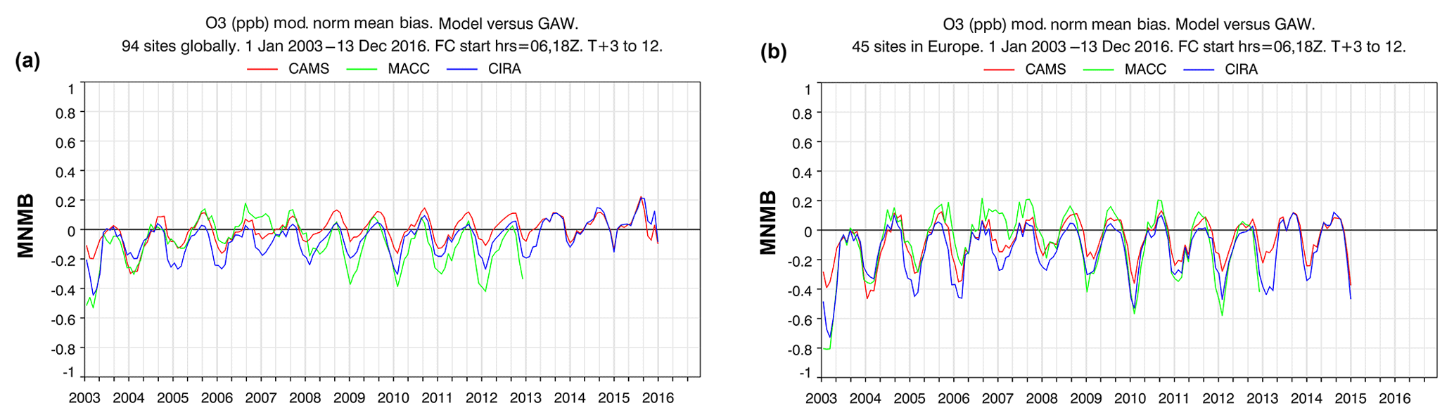
Figure 11Time series of monthly mean surface ozone MNMB between the three reanalyses and GAW O3 data averaged over (a) the globe and (b) Europe. Globally about 60–70 stations were available from 2003 to 2014, dropping to about 40–50 in 2015 and then dropping steeply to only a few during 2016. In Europe, the number dropped from 25–35 in 2003–2014 to 17–19 in 2015. CAMSRA is shown in red, CIRA in blue and MACCRA in green.
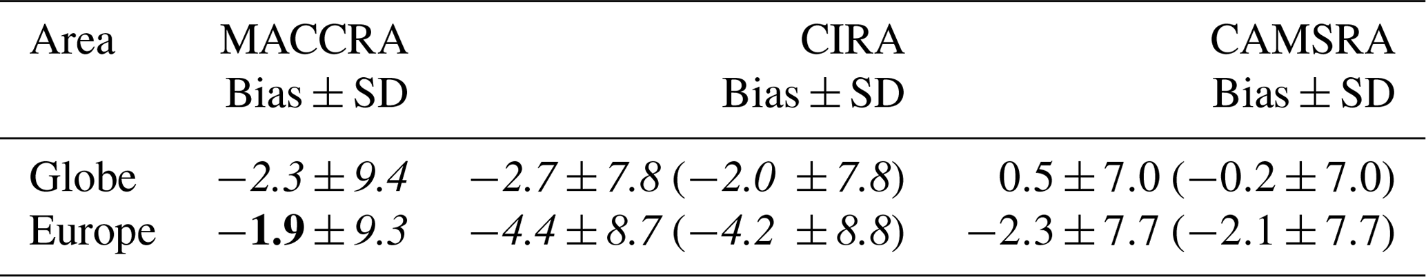
To finish the O3 validation we look at surface ozone data. Figure 11 shows time series of MNMB of the reanalyses with respect to ground-based surface observations from the WMO's Global Atmosphere Watch (GAW) programme (e.g. Oltmans and Levy II, 1994) averaged globally and for Europe. The GAW observations represent the global background away from the main polluted areas. Detailed information on GAW can be found in GAW reports no. 209 (available from https://www.wmo.int/pages/prog/arep/gaw/documents/Final_GAW_209_web.pdf, last access: 15 March 2019). GAW O3 data have a precision of ±1 ppbv. Table 4 shows the global and Europe mean biases and their standard deviations from all three reanalyses averaged over the periods 2003–2012 and 2003–2016 for CAMSRA and CIRA. In the global mean CAMSRA agrees with the surface data to within 10 % for most years. The biases are generally negative during the first half of the year and positive during the second half. MACCRA has larger negative biases after 2008, and CIRA has larger negative biases from 2003 to 2012. Surface O3 in CAMSRA is higher than in CIRA so that the global mean biases during boreal spring are smaller, but the positive global mean biases during boreal summer are larger. After spring 2013 CAMSRA and CIRA are very close. During 2003 CIRA and MACCRA have a considerably larger bias than CAMSRA. This is also seen over Europe and North America and was also seen in ozone in the free troposphere (Fig. 9). In Europe CAMSRA has biases between −40 % and +10 %. All three reanalyses show an underestimation of surface O3 during boreal spring and better agreement with the observations during summer, when the bias is positive. The negative springtime bias is a known problem in the CAMS system and is generally smaller in CAMSRA than CIRA. The largest negative bias in CAMSRA is seen during 2004 (when no O3 profile data were assimilated). CAMSRA has the smallest global mean bias against GAW data of the three reanalyses averaged over the period 2003–2012 (0.51±6.95 ppb for CAMSRA, ppb for CIRA and ppb for MACCRA) and also has smaller biases than CIRA for the period 2003–2016 (see Table 4). The mean bias for Europe (2003–2012) is ppb for MACCRA, ppb for CIRA and ppb for CAMSRA.
Table 4Mean biases and standard deviations from MACCRA, CIRA and CAMSRA relative to GAW surface O3 data (shown in Fig. 11; in ppb). The values are calculated for the period 2003–2012, and the values in brackets are calculated for CIRA and CAMSRA for the period 2003–2016. Numbers in italics mark where MACCRA or CIRA have larger biases or a larger standard deviation than CAMSRA; numbers in bold mark where their values are smaller.
In summary, it can be said that for O3 CAMSRA is temporally more consistent than the older reanalyses and has smaller biases compared with independent observations (see Tables 3 and 4). The comparisons also show that it is not advisable to concatenate the older reanalyses with more recent years from CAMSRA because the datasets are too different and that users should use only data from CAMSRA if they are interested in the complete period from 2003 to 2016. There are some periods with slightly degraded quality (bigger biases) that the user should be aware of. These include the Arctic and Antarctic free troposphere during 2003 because MIPAS and SCIAMACHY data or poorer quality were assimilated, the period between the end of March and the beginning of August 2004, when no profile data were available for assimilation, and a change in bias after 2013 that is still under investigation. The underestimation of surface O3 seen in the CAMS system in the NH during boreal spring is reduced in CAMSRA compared with the older reanalyses.
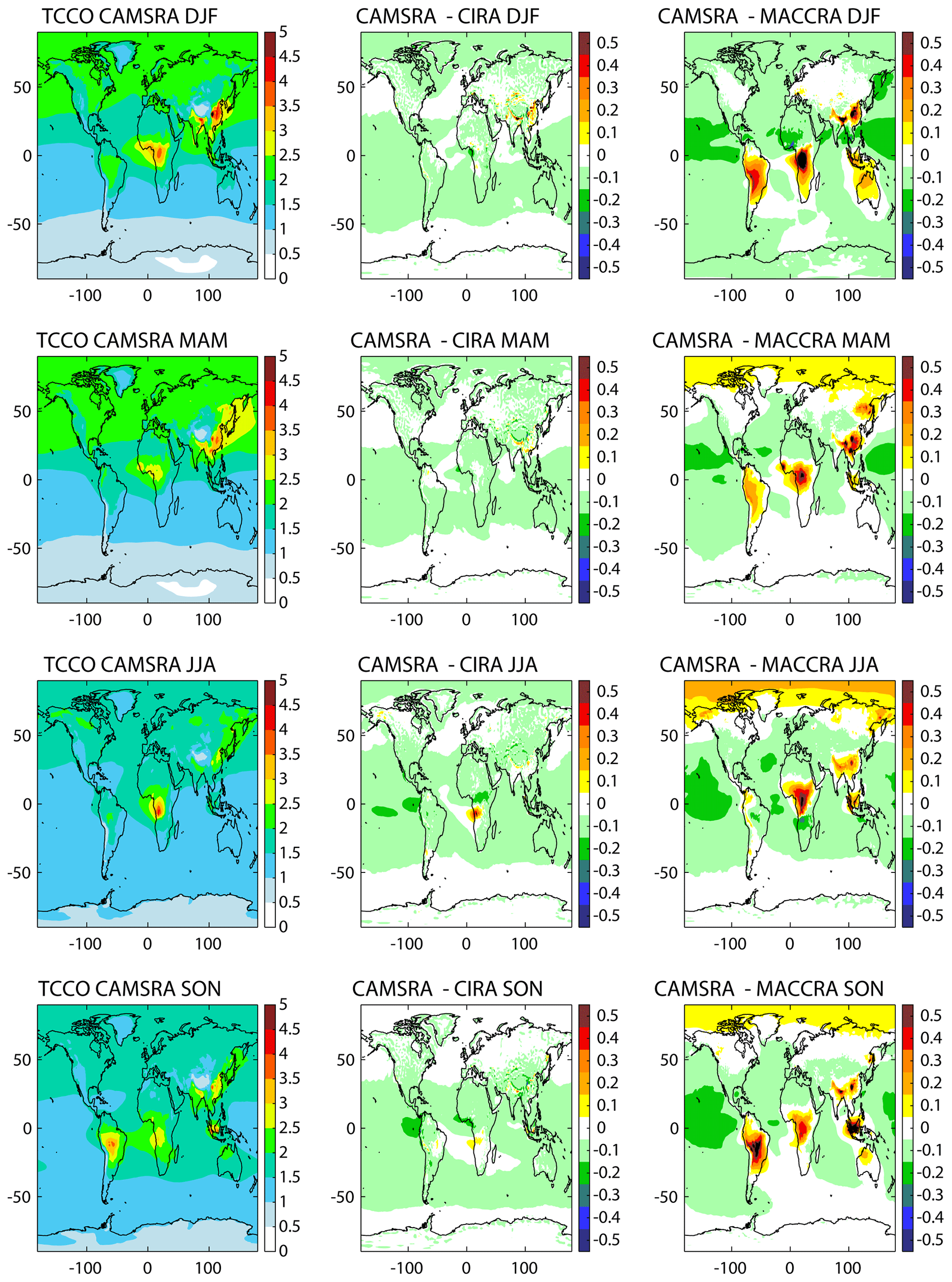
Figure 12Seasonally averaged TCCO from CAMSRA (2003–2016, left), difference between CAMSRA and CIRA (middle), and difference between CAMSRA and MACCRA (right, 2003–2012 only) in 1018 molec cm−2 for the seasons DJF (row 1), MAM (row 2), JJA (row 3) and SON (row 4).
4.2 Carbon monoxide
Next, we look at CO fields from the reanalyses and compare them with independent observations. Figure 12 shows the seasonally averaged TCCO fields from CAMSRA and the differences between this dataset and CIRA and MACCRA. The TCCO differences between CAMSRA and CIRA are small (below 0.1×10¹⁸ molec cm−2, < 5 %) with CAMSRA generally lower than CIRA, apart from African biomass burning areas south of the Equator in JJA and parts of Southeast Asia in DJF and MAM. The largest relative differences (of up to 15 %, not shown) are found over the tropical oceans where background values are small. The differences between CAMSRA and MACCRA are larger. CAMSRA is lower than MACCRA over the oceans (0.1–0.2×10¹⁸ molec cm−2, relative differences mainly < 15 %) and is much higher over biomass burning areas, e.g. South America, Africa, Southeast Asia, Indonesia, Australia in DJF and boreal fires in Siberia in MAM and JJA, with differences up to 0.5×10¹⁸ molec cm−2 (corresponding to maximum relative differences of up to 30 % over Indonesia). These difference plots show that the choice of fire emissions used in the reanalysis has a large impact on the TCCO field. In MACCRA these came from GFED (van der Werf et al., 2010) for the period 2003-2008 and GFASv1.0 from 2008 to 2012 (Kaiser et al., 2012), while in CAMSRA and CIRA, GFASv1.2 was used throughout from 2003 to 2016 (see Table 1 and Fig. 4). As for O3, the differences between the reanalyses are too large to allow the user to concatenate recent years from CAMSRA with earlier years from the other reanalyses.
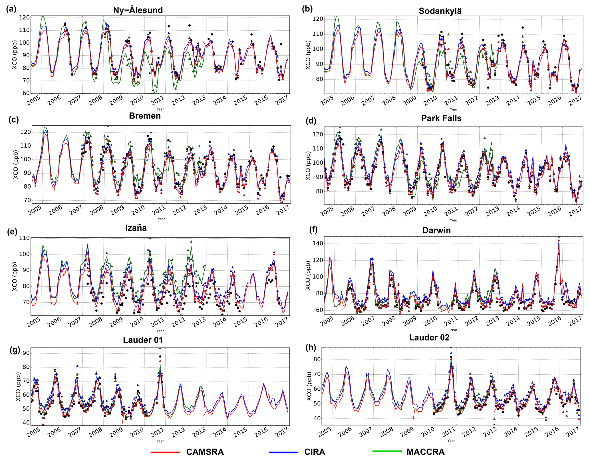
Figure 13Column-averaged CO (XCO; in ppb) at several TCCON stations. Monthly mean observations are shown by the black dots, and corresponding monthly mean XCO columns calculated using the TCCON averaging kernels are shown by the red (CAMSRA), blue (CIRA) and green (MACCRA) triangles. The continuous lines are the monthly XCO for the three reanalyses. Shown are data for (a) Ny-Ålesund, (b) Sodankylä, (c) Bremen, (d) Park Falls, (e) Izaña, (f) Darwin, (g) Lauder 2004–2010 and (h) Lauder 2010–2016.
Table 5TCCON stations used in this paper and mean biases and standard deviations from MACCRA, CIRA and CAMSRA (shown in Fig. 13; in ppb). The values for CIRA and CAMSRA are calculated for the period 2003–2016, and the values for MACCRA are calculated for the period 2003–2012. Numbers in italics mark where MACCRA or CIRA have larger biases or standard deviation than CAMSRA, and numbers in bold mark where their values are smaller.
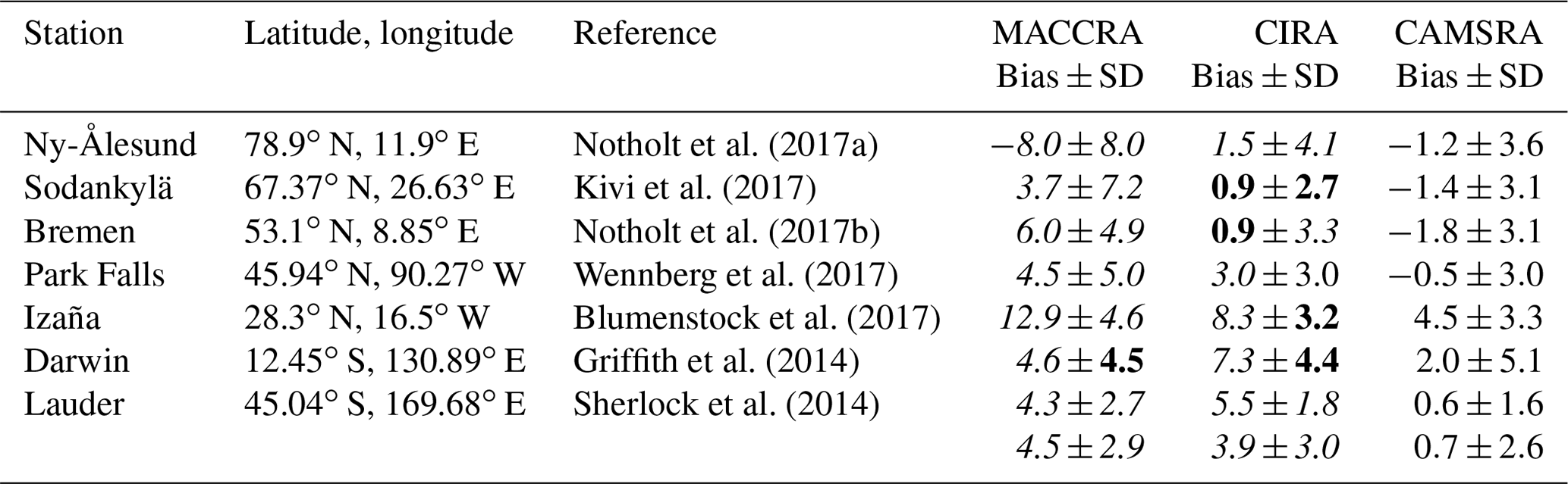
To validate CO from the reanalysis with independent observations, in Fig. 13 we first compare our data with observations from Total Carbon Column Observing Network stations (TCCON, GGG2014 data; Wunch et al., 2011, see http://www.tccon.caltech.edu, last access: 15 March 2019) at six sites covering latitudes from the Arctic to Australia (see Table 5). The TCCON stations measure the column-averaged dry molar fraction CO amount (XCO) and have an absolute accuracy of about 4 % (Wunch et al., 2010). Figure 13 shows very good agreement of CAMSRA with the independent observations, in particular for the year-to-year variability. The mean bias and standard deviations of the three reanalyses against the TCCON data are given in Table 5 and show that the mean biases of CAMSRA are reduced at all stations compared to MACCRA. CAMSRA is slightly lower than CIRA, with smaller biases and standard deviation at all stations except Bremen and Sodankylä. Particularly in the tropics and SH, the biases and standard deviations are reduced much in CAMSRA. CAMSRA captures the seasonal cycle well at all stations. Especially the summer minimum (e.g. boreal summer in NH or austral summer in SH) is better captured in CAMSRA than in CIRA. CAMSRA underestimates XCO at the NH stations Ny-Ålesund, Sodankylä, Bremen and Park Falls (biases < −2 ppb) and overestimates it in the tropics (Izaña, < 5 ppb; Darwin, < 2 ppb) and in the SH (Lauder, < 1 ppb). CIRA slightly overestimates XCO in the NH (< 3 ppb) and has a larger positive bias than CAMSRA in the tropics and SH (up to 8 ppb).
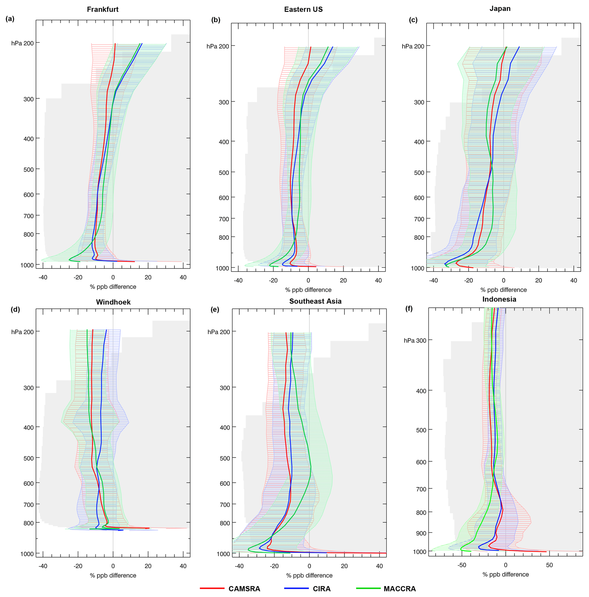
Figure 14Mean relative CO bias (in %) between the reanalyses and IAGOS aircraft data for CAMSRA (red), CIRA (blue) and MACCRA (green) at (a) Frankfurt, (b) eastern US airports, (c) Japanese airports, (d) Windhoek, (e) Southeast Asian airports and (f) Indonesian airports (note the different scale of the axis for f). The shaded areas show plus or minus 1 standard deviation. For CAMSRA and CIRA the average is calculated over the period 2003–2016, and for MACCRA the average is calculated only for 2003–2012.
To also assess the vertical structure of the CO analysis fields, in Fig. 14 we compare model fields with CO profiles from MOZAIC (Measurements of ozone, water vapour, carbon monoxide and nitrogen oxides by airbus in-service aircraft) and IAGOS (In-service Aircraft for a Global Observing System) observations from instruments mounted on commercial aircraft. The MOZAIC–IAGOS CO data have an accuracy of ±5 ppbv, a precision of ±5 % and a detection limit of 10 ppbv (Nedelec et al., 2003). We use CO profiles obtained during take-off and landing to evaluate the CO reanalysis fields. The profiles at the NH midlatitude airports (Frankfurt, eastern US and Japan) show that all three reanalyses underestimate CO in the free troposphere but agree to within 10 % with the aircraft data. A larger underestimation is found in the boundary layer. Here, MACCRA has the largest negative bias. This underestimation in MACCRA was noted previously (Inness et al., 2013) and led to a modification of increased wintertime road traffic emissions over North America and Europe in the MACCity emissions (Stein et al., 2014). These modified emissions are used in CAMSRA and CIRA. CAMSRA and CIRA are generally closer to each other in the lower troposphere than to MACCRA. This area is less impacted by the assimilated MOPITT TIR retrievals that have the largest sensitivity to CO in the mid-troposphere (Deeter et al., 2013) and more by emissions and differences in the chemistry schemes, which are more similar in CAMSRA and CIRA than in MACCRA. In the upper troposphere CAMSRA has the lowest mean bias, while CIRA and MACCRA overestimate CO above about 300 hPa. At Windhoek, all reanalyses underestimate the aircraft data. Here CAMSRA and MACCRA have a smaller bias than CIRA below 650 hPa, but CIRA has a smaller bias above 500 hPa. Over Southeast Asia all reanalyses show a large underestimation in the boundary layer, with MACCRA having the largest bias of up to −35 %. In the free troposphere all reanalyses underestimate CO but have a smaller bias than near the surface. MACCRA has the smallest bias in the free troposphere (biases of less than −5 % between 650 and 400 hPa). This could be the result of assimilating the Infrared Atmospheric Sounding Interferometer (IASI) TCCO data (George et al., 2009; Clerbaux et al., 2009) in MACCRA in addition to MOPITT. Like MOPITT, IASI CO retrievals are most sensitive to CO in the mid-troposphere and could add an extra constraint on CO here when more observations are being assimilated, as IASI has a better coverage than MOPITT (e.g. Barré et al., 2015). Over Indonesia CAMSRA and CIRA have smaller biases than MACCRA below 700 hPa. This is likely due to differences in the fire emissions. At Windhoek, Southeast Asia and Indonesia, CAMSRA and CIRA overestimate surface CO. This overestimation is also seen in comparison with GAW surface CO data at Cape Point (not shown).
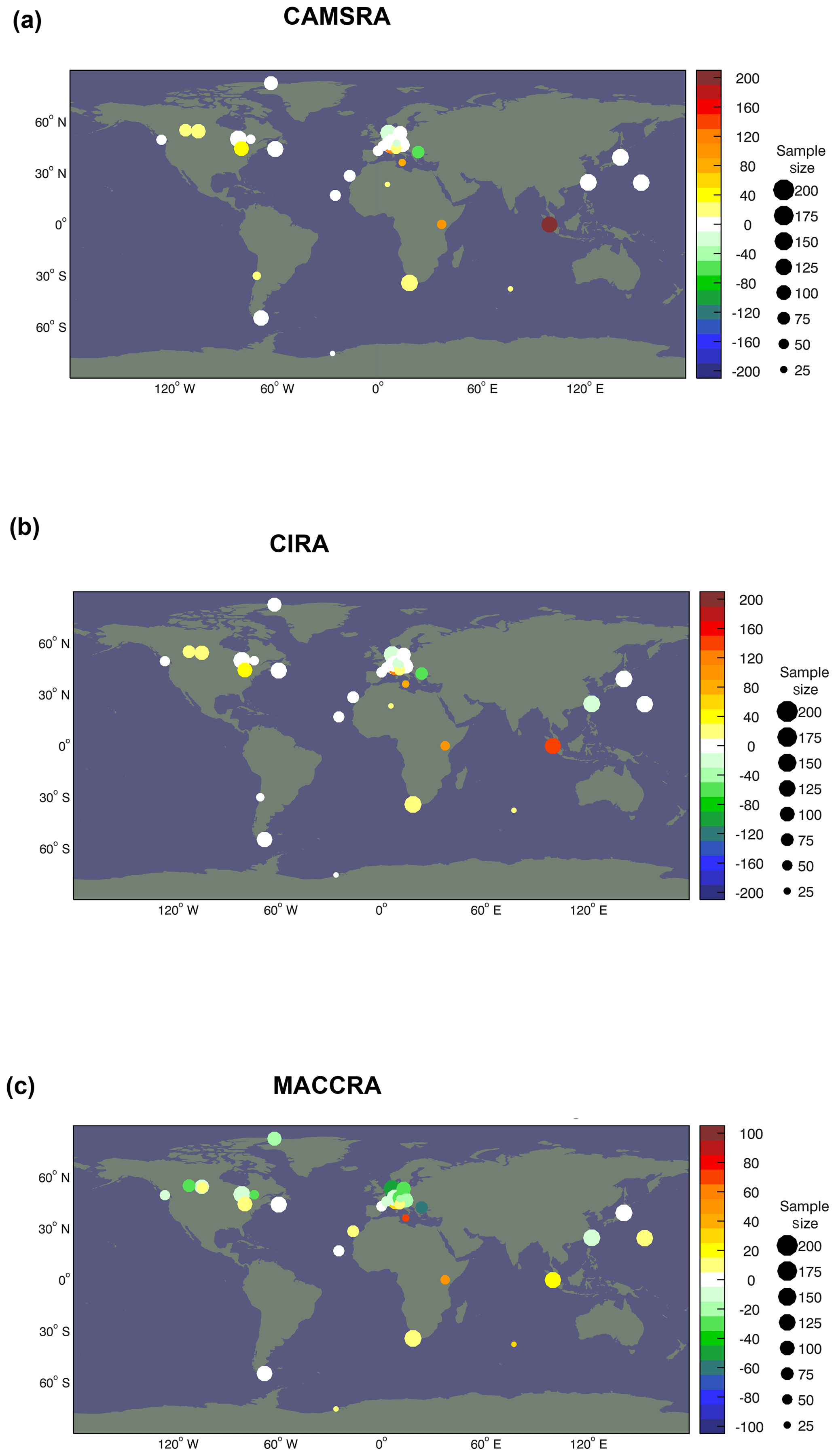
Figure 15Mean CO bias (in ppb) between the three reanalyses, and GAW surface observations for (a) CAMSRA, (b) CIRA and (c) MACCRA. For CAMSRA and CIRA the average is calculated over the period 2003–2016, and for MACCRA it is only calculated for 2003–2012.
Next, we look at surface CO data. Figure 15 shows maps of mean biases of surface CO against GAW observation. The data are averaged over the period 2003–2016 for CAMSRA and CIRA and 2003–2012 for MACCRA. The uncertainty of GAW CO data is between 2 ppbv for marine boundary layer sites and 5 ppbv for continental sites that are influenced by regional pollution (GAW report 192, available from http://www.wmo.int/pages/prog/arep/gaw/documents/GAW_192_WMO_TD_1551_web.pdf, last access: 15 March 2019). The biases in CAMSRA and CIRA are less than 10 % for many stations, with slightly larger positive biases for some North American stations and slightly larger negative biases for some European stations. MACCRA has larger negative biases over North America and Europe. CAMSRA shows a larger positive bias than the other two reanalyses at the Indonesian station of Bukit Koto Tabang. Looking at a time series at this location (Fig. 16d) we see that the station is strongly influenced by high CO events during years with intense biomass burning (2004, 2006, 2014 and 2015), with the largest peaks in 2014 and 2015, when CAMSRA is higher than CIRA. This is after the end of MACCRA, which only covered the period from 2003 to 2012. It has to be assessed if this overestimation is the result of GFAS emission factors that are too large for CO.
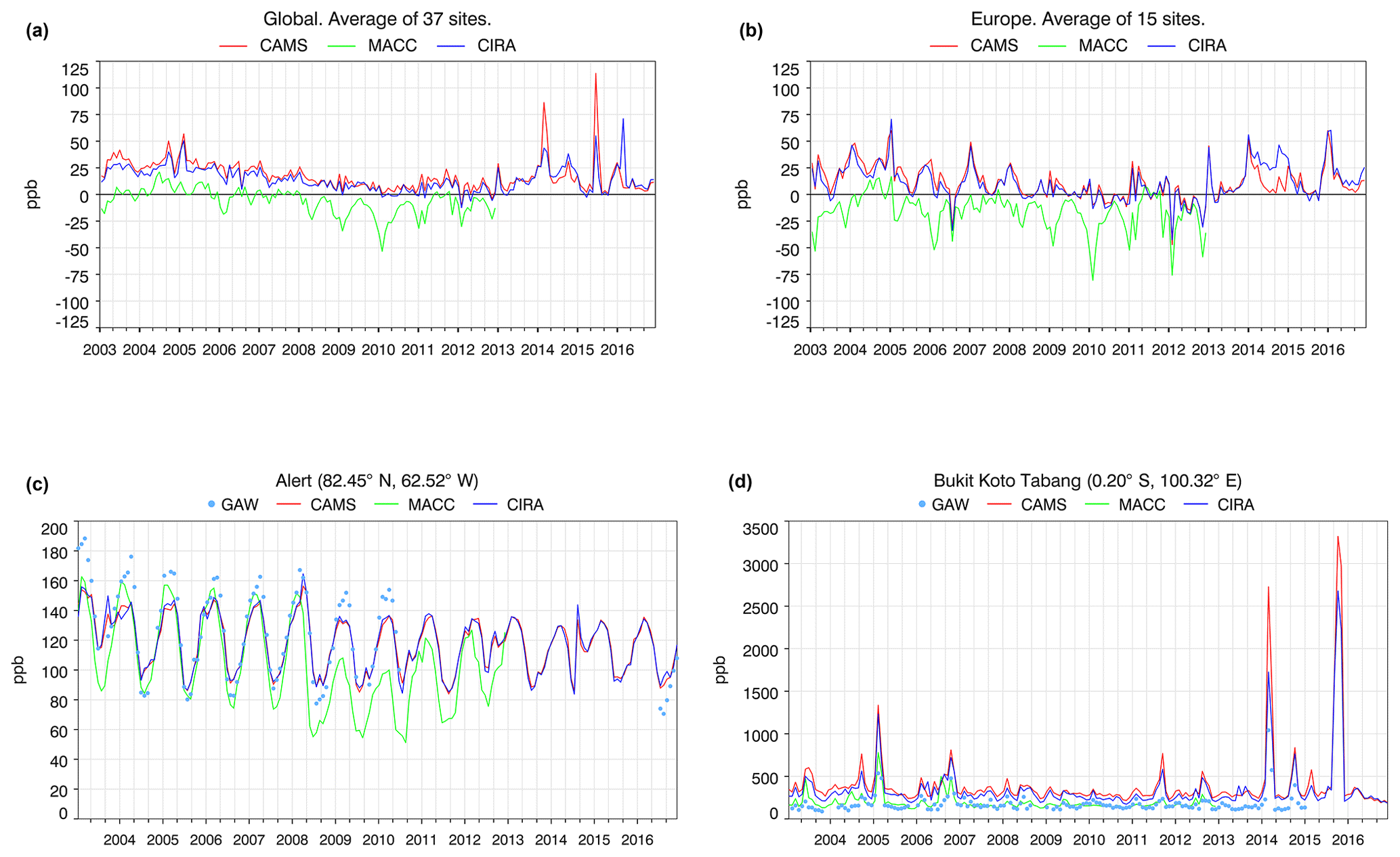
Figure 16Top panels depict time series of monthly mean surface CO bias (in ppb) between the three reanalyses and GAW CO data averaged over (a) the globe and (b) Europe. Between 15 and 30 stations were available between 2003 and 2016, with largest number between 2008 and 2014 and smaller numbers in the earlier and later years. (c, d) Time series of monthly mean CO from GAW (blue dots), CAMSRA, CIRA and MACCRA (in ppb) at (c) Alert and (d) Bukit Koto Tabang. CAMSRA is shown in red, CIRA in blue and MACCRA in green.
Table 6Mean biases and standard deviations from MACCRA, CIRA and CAMSRA relative to GAW surface CO data (shown in Fig. 16; in ppb). The values are calculated for the period 2003–2012, and the values in brackets are calculated for CIRA and CAMSRA for the period 2003–2016. Numbers in italics mark where MACCRA or CIRA have larger biases or standard deviation than CAMSRA, and numbers in bold mark where their values are smaller.
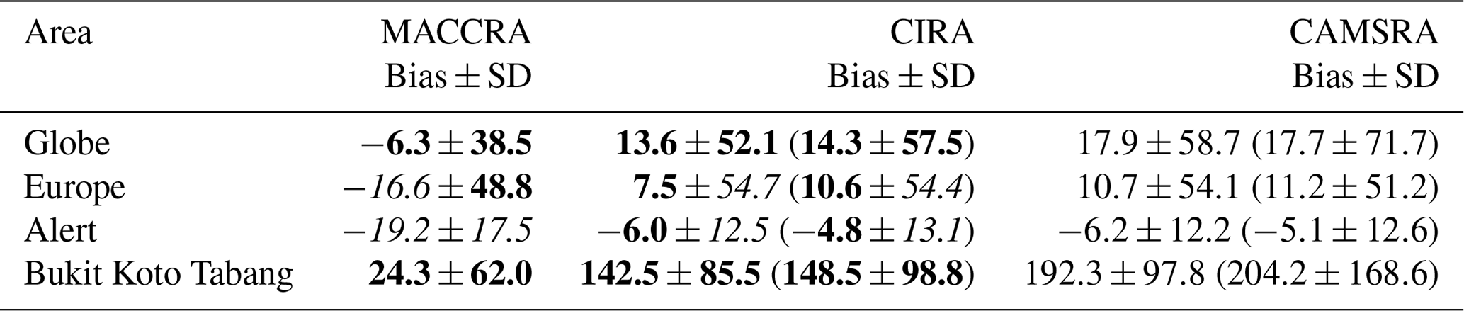
Figure 16 shows time series of monthly mean CO surface biases of the reanalyses with respect to GAW observations averaged over the globe and Europe as well as time series of absolute surface CO values at the Arctic Alert station and the Indonesian Bukit Koto Tabang station. Table 6 shows the corresponding mean biases of the three reanalyses and their standard deviations. The agreement of MACCRA with GAW CO data over Europe (Fig. 16b) is worse than for the other two reanalyses with a large underestimation during boreal winter. This bias was already documented in Inness et al. (2013) and Flemming et al. (2017b). The negative bias of MACCRA increases after April 2008, when the assimilation of IASI CO retrievals started in MACCRA (see Inness et al., 2013), and is particularly pronounced at high northern latitudes (e.g. time series at Alert; Fig. 16c), where the mean bias for 2003–2012 is ppb for MACCRA, ppb for CIRA and ppb for CAMSRA. The mean bias for MACCRA over Europe for the period 2003–2012 is ppb, while CAMSRA (10.7±54.0 ppb) and CIRA (7.5±54.7 ppb) both have smaller positive biases. The average global mean bias for the period 2003–2012 is negative for MACCRA ( ppb). Larger and positive global mean biases for 2003–2012 are found for CIRA (13.6±52.1 ppb) and CAMSRA (17.9±71.7 ppb). The larger global mean bias for CAMSRA is dominated by the large overestimation of surface CO over Indonesia during years with high biomass burning activity (see Fig. 16d). The differences between MACCRA and the other reanalyses are likely the result of using GFED instead of GFAS fire emissions.
In summary, CO from CAMSRA has a good seasonal cycle and captures the interannual variability observed by TCCON data well. CAMSRA has smaller biases relative to TCCON data than the older reanalyses at most stations. There is a low bias with respect to IAGOS aircraft data in the lower troposphere over NH midlatitudes, Southeast Asia and Indonesia. This is a persistent feature of the CAMS system, and more work is needed to assess if it is a model problem or due to problems with the emissions. CAMSRA generally agrees better with GAW surface observations than MACCRA over much of the globe (e.g. Europe and North America) but has larger biases relative to GAW over Indonesia which lead to larger global mean biases when averaged over 2003–2012 or 2003–2016. CAMSRA is more similar to CIRA than MACCRA because of differences in the emissions, chemistry schemes and assimilated data. It is therefore not possible to use a climatology based on the MACCRA data and recent years from CAMSRA to calculate anomalies, for example.
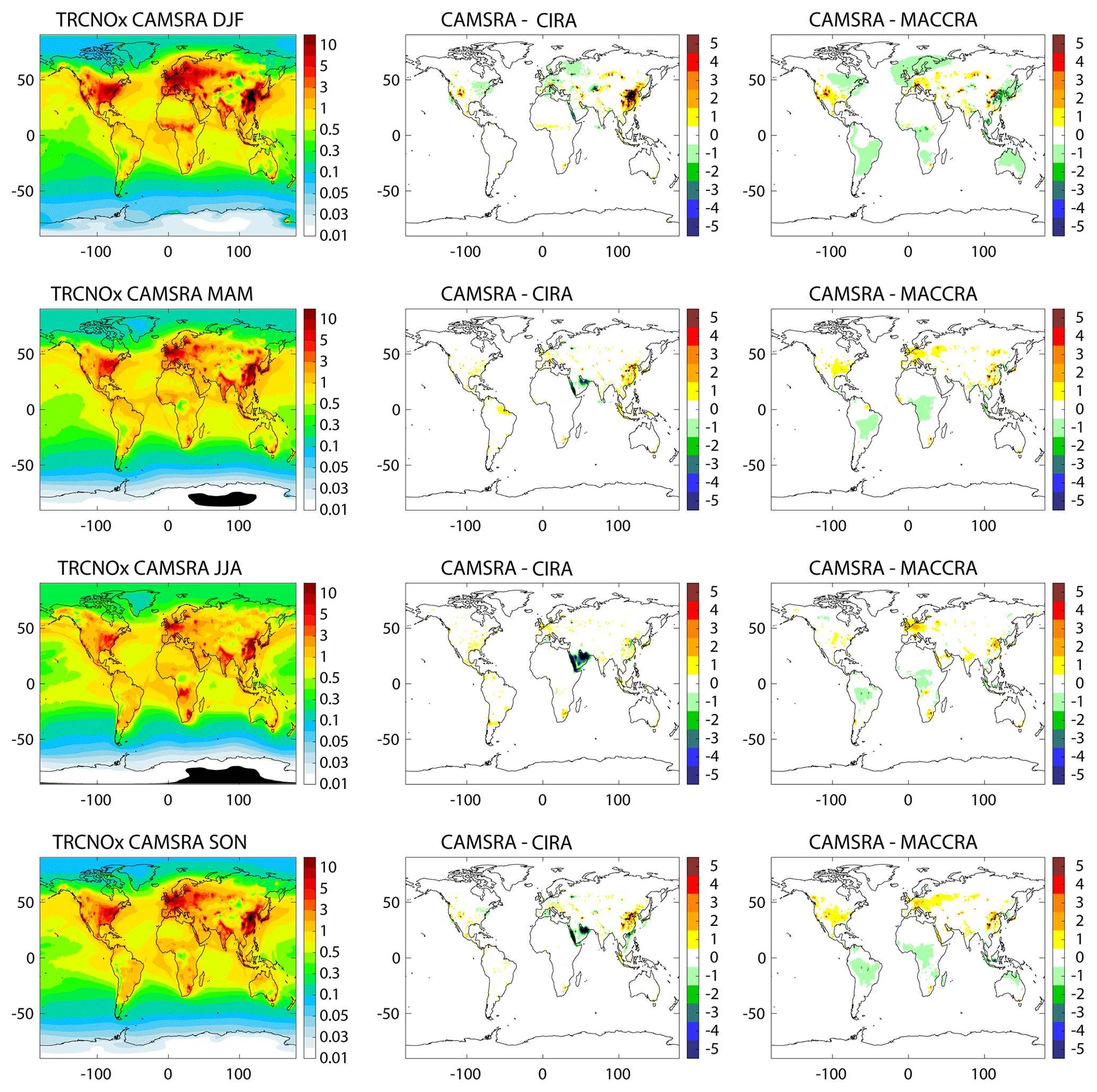
Figure 17Seasonally averaged TRCNOx in 1015 molec cm−2 from CAMSRA (2003–2016, left), the differences between CAMSRA and CIRA (middle), and the differences between CAMSRA and MACCRA (right, 2003–2012 only) for the seasons DJF (row 1), MAM (row 2), JJA (row 3) and SON (row 4).
4.3 Nitrogen dioxide
The final reactive gases species discussed in this paper is NO2. Validation of NO2 with independent observations, especially surface observations, is difficult because of the short lifetime and large variability of the concentrations. First, we compare the seasonally averaged tropospheric column NOx (TRCNOx) fields from CAMSRA, CIRA and MACCRA in Fig. 17. Figure 17 shows that CAMSRA has a realistic TRCNOx distribution with high NOx columns in the NH in areas affected by anthropogenic emissions and also in boreal and tropical biomass burning areas. The largest TRCNOx values are found in DJF in the NH, when emissions are largest and the NOx lifetime is longest. In Africa, a realistic seasonal cycle is found, with a maximum in the Sahel in DJF and maximum values south of the Equator in JJA related to the seasonality of biomass burning. NOx columns over South America are smaller than over Africa, with the largest values found in JJA and SON because deforestation fires and agricultural fires mainly occur south of 10∘ S during August–October, with a peak in September.
Differences between CAMSRA and CIRA are due to model changes but are also due to the assimilation of the tropospheric column NO2 retrievals from SCIAMACHY, OMI and GOME-2 in CAMSRA (see Table 2). No NO2 retrievals were assimilated in CIRA. Over large parts of the world the differences are small. The largest positive differences are seen over Southeast Asia, particularly during DJF. Over Europe and the eastern US, CAMSRA has lower TRCNOx values than CIRA during DJF. The fact that the largest differences in the NH are seen during DJF suggests that this is at least partly due to the impact of the assimilation of the satellite data. While the impact of the NO2 assimilation is generally small because of the short lifetime of NO2, it was found to have a larger impact during winter and spring, when the lifetime is longer than during summer (see Figs. S5 and S6 and Inness et al., 2015). Furthermore, by assimilating NO2 retrievals from satellites with different overpass times (09:30 LT for GOME-2, 10:00 LT for SCIAMACHY and 13:30 LT for OMI), the impact of the assimilation is likely to be increased. CAMSRA has much lower values than CIRA over the Arabian Peninsula, with the largest differences found in JJA. This reduction is not due to the assimilated data but due to model changes, i.e. the coupling with aerosol in the chemistry scheme (see Sect. 2.1) that leads to faster NOx removal and reduces the positive bias noted before in the CAMS system in this area when evaluating against satellite NO2 observations (not shown). The differences between CAMSRA and MACCRA are mainly negative over land in the tropics and positive over areas of anthropogenic emissions apart from the eastern US and parts of China in DJF. These differences are a result of the different chemistry schemes and biomass burning emissions used in CAMSRA and MACCRA as well as the assimilation of NO2 retrievals from different instruments (only SCIAMACHY assimilated in MACCRA).
It is difficult to find independent NO2 data for validation which are representative for the grid box size of the CAMSRA global reanalysis. We use the following two datasets for validation: (1) a satellite-based tropospheric column NO2 dataset and (2) surface NO2 measurements from selected GAW stations in Europe. GAW stations aim to have an uncertainty of about 3 % for monthly mean data (Penkett et al., 2011). As the number of GAW stations measuring NO2 is small and drops considerably with time during the period of interest, it is not meaningful to look at time series of area means. We therefore restrict our validation to four European GAW stations that have observations for most of the period from 2003 to 2016. The dataset (1) is produced by the University of Bremen based on SCIAMACHY–Envisat NO2 satellite retrievals (IUP-UB v0.7, before April 2012; Richter et al., 2005) and GOME-2 and Metop-A NO2 satellite retrievals (IUP-UB v1.0, from April 2012 to the end of 2016; Richter et al., 2011). The retrieval product used for validation is different to the SCIAMACHY and GOME-2 NO2 retrievals that are assimilated in CAMSRA (which are produced by the ACSAF; see Table 2). Despite the retrievals being based on the same Level 1 spectral irradiance data, the retrieval procedures are completely independent, from the spectral fit to the assumptions made on the a priori data used for the air mass factor calculations. In the absence of other independent validation data for tropospheric NO2 columns, they can still provide a critical evaluation of the model performance on a global scale. The satellite data are always taken at the same local time, roughly 10:00 LT for SCIAMACHY and 09:30 LT for GOME-2, and with a clear sky only. Model data are vertically integrated, interpolated linearly in time to the observation time of SCIAMACHY (which is expected to lead to minor uncertainties when comparing to GOME-2 observations in Fig. 18 below) and then sampled spatially to match the satellite data. Model data were treated with the same reference sector subtraction approach as the satellite data. Uncertainties in NO2 satellite retrievals are large and depend on the region and season. Winter values in midlatitudes and high latitudes are usually associated with larger error margins. As a rough estimate, systematic uncertainties in regions with significant pollution are on the order of 20 %–30 %.
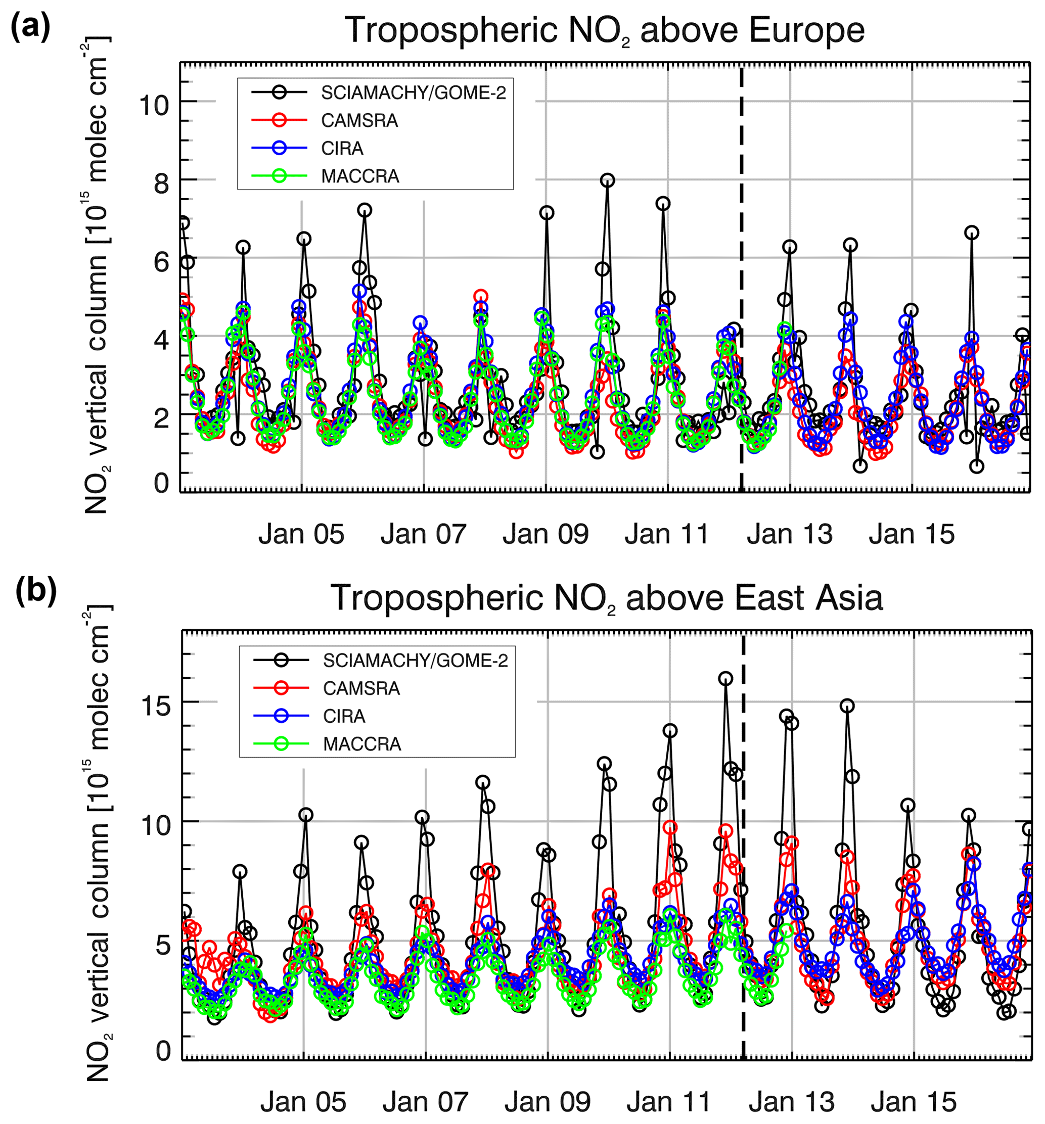
Figure 18Time series of tropospheric column NO2 from the three reanalyses and IUB tropospheric NO2 retrievals in 1015 molec cm−2 averaged over (a) Europe and (b) East Asia. CAMSRA is shown in red, CIRA in blue, MACCRA in green and the observations in black.
Figure 18 shows time series of tropospheric column NO2 from the Bremen satellite dataset (), CAMSRA, CIRA and MACCRA averaged over Europe and East Asia for the period from 2003 to 2016. The figure illustrates that, while the seasonality of NO2 (with low values during summer and high values during winter) is captured in both areas, there is generally an underestimation of the seasonal cycle, mainly due to an underestimation of the wintertime maximum. This underestimation could be related to an underestimation of anthropogenic emissions or uncertainties in the photochemistry of the models and is particularly pronounced over East Asia. Over Europe the differences between the three reanalyses are small; over East Asia they are larger. Over East Asia in 2003, the CAMS reanalysis shows a strong variation in values from one month to the next and fails to reproduce the observed seasonality. This is due to assimilating SCIMACHY NO2 data of degraded quality during 2003 in CAMSRA (see Fig. S5a). The Bremen dataset shows an increase in the wintertime maximum NO2 values over East Asia until 2012–2014 and a decrease in the later years. This behaviour is reproduced better in CAMSRA than in CIRA and MACCRA, though the maximum values are still underestimated. This improvement is the result of assimilating more NO2 satellite data, in particular data from satellites with different overpass times, in CAMSRA. It is not seen in a control run without data assimilation (not shown). However, the magnitude of the positive trend up to 2012 and of the negative trend in the recent years is still underestimated by CAMSRA, and the observed decrease after 2014 is not reproduced by the three reanalyses.

Figure 19Time series of monthly mean surface NO2 from CAMSRA (red), CIRA (blue), MACCRA (green) and GAW surface observations (blue dots) for (a) Łeba, (b) Jarczew, (c) Hohenpeißenberg and (d) Payerne (in ppb). The latitude and longitude of the stations are given in the plot titles.
Figure 19 shows time series of surface NO2 from CAMS, CIRA and MACCRA, with GAW surface observations at four European stations, and Table 7 lists the corresponding mean biases and their standard deviations. Overall, the reanalyses reproduce the observed mean values and the seasonal variability well. At Łeba (on the Baltic coast) all three reanalyses capture the annual cycle well, with high NO2 concentrations during the winter and lower concentrations during the summer. MACCRA underestimates the summertime minimum more than the other two reanalyses. Averaged over the years 2003–2012 CAMSRA has the smallest bias, 0.0±0.6 ppb, compared to ppb for MACCRA and 0.1±0.6 ppb for CIRA. At Jarczew (Poland) both CAMSRA and MACCRA capture the low summertime NO2 values better than CIRA, which has a positive bias during summer, while the wintertime NO2 maxima are more similar in the three reanalyses. Overall, CAMSRA agrees best with the GAW data here, with the smallest mean bias and standard deviation (see Table 7). At Hohenpeißenberg in southern Germany all reanalyses underestimate the summer minimum and struggle to capture some of the high winter values between 2008 and 2012. CIRA underestimates the winter maximum values most, while CAMSRA and MACCRA agree better with the observations during winter, especially during the first half of the time series. MACCRA has the smallest mean bias ( ppb), followed by CAMSRA ( ppb) and CIRA ( ppb) for the period 2003–2012. At Payerne (Switzerland), MACCRA strongly underestimates the GAW observations (mean bias of ppb), while CAMSRA (mean bias of ppb) and CIRA (mean bias of ppb) capture the annual cycle reasonably well, in particular the summer minimum.
Table 7Monthly mean surface NO2 biases and standard deviations from MACCRA, CIRA and CAMSRA relative to GAW surface NO2 data (shown in Fig. 19; in ppb). The values are calculated for the period 2003–2012, and the values in brackets are calculated for CIRA and CAMSRA for the period 2003–2016. Numbers in italics mark where MACCRA or CIRA have larger biases or standard deviation than CAMSRA, and numbers in bold mark where their values are smaller.
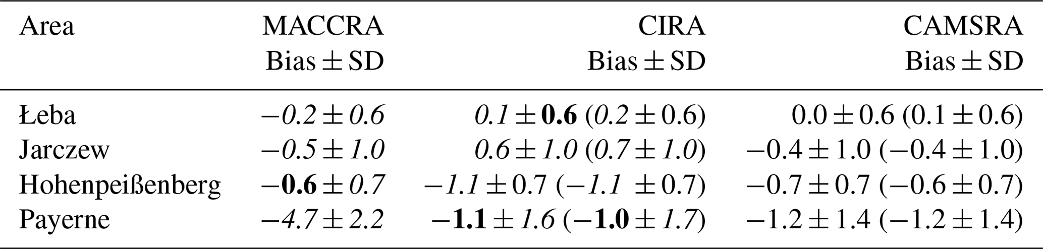
In summary, we find that CAMSRA shows some improvements in the tropospheric NO2 column (relative to a dataset based on SCIMACHY and GOME-2A data) compared with the older two reanalyses, especially over East Asia, where the assimilation of (more) NO2 retrievals reduces the bias between the reanalysis and the data. However, the tropospheric NO2 columns are still underestimated in CAMSRA over East Asia and Europe, particularly the wintertime maxima. This is a long-standing problem of the CAMS system, and it is hoped that work which has started to include an emission inversion capability in the CAMS system will improve this in the future. We find changes in NO2 compared with CIRA (particularly over the Arabian Peninsula), which are the result of coupling with aerosol in the CAMSRA chemistry scheme that leads to faster NOx removes and a reduced positive bias in those areas. Compared with GAW surface NO2 observations at four European stations CAMSRA reproduces the monthly mean values and the seasonal variability well, with some underestimation of wintertime maximum values.
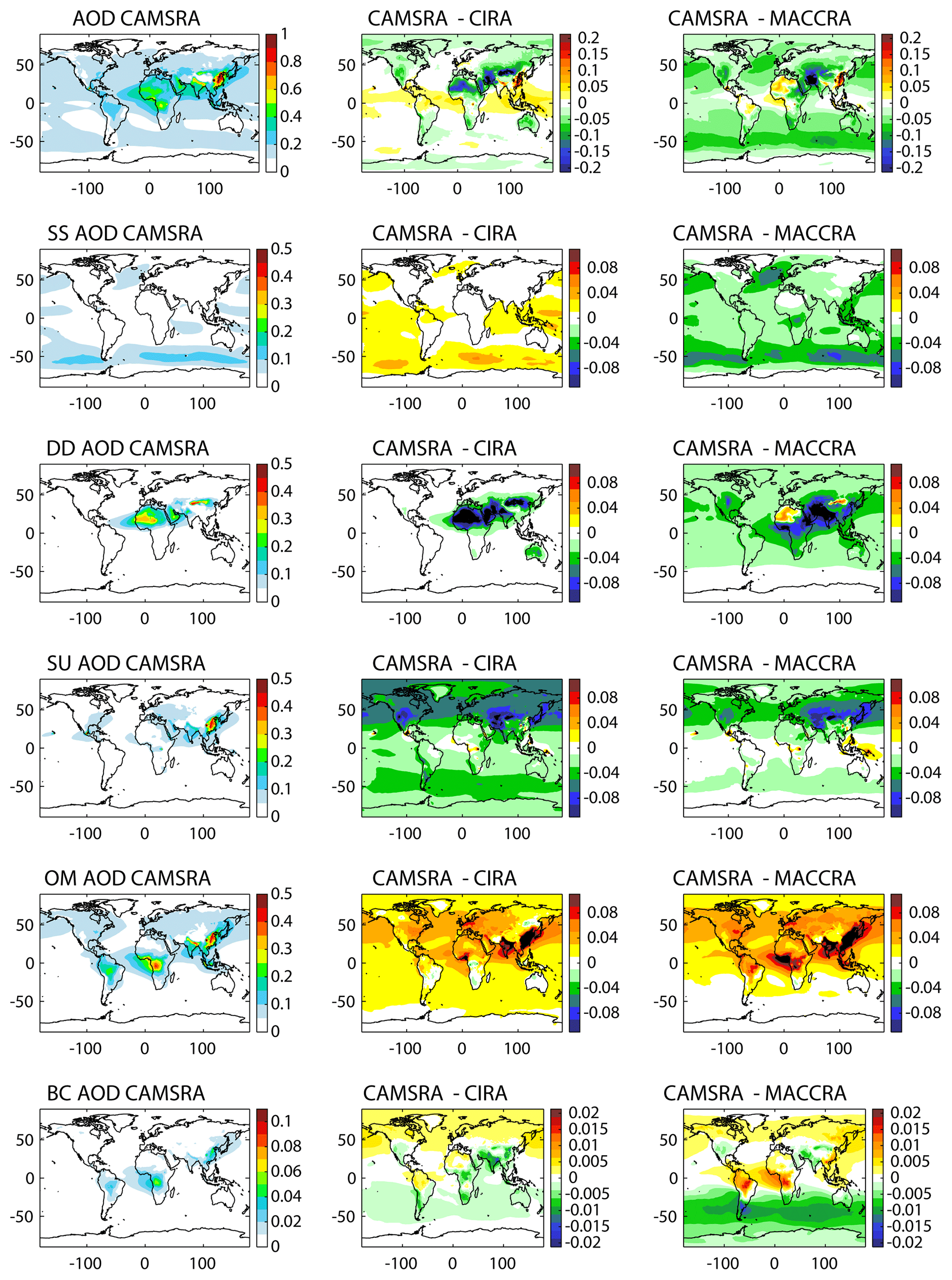
Figure 20Annually averaged AOD species from CAMSRA (2003–2016, left), difference between CAMSRA and CIRA (middle), and difference between CAMSRA and MACCRA (right, 2003–2012 only) for total AOD (row 1), sea salt (row 2), desert dust (row 3) and sulfates (row 4), organic matter (row 5), and black carbon (row 60). AOD is unitless.
4.4 Aerosols
The final validation section looks at aerosol fields from the three reanalyses. Several model changes were included in the version of the IFS used to produce CAMSRA to address issues identified in CIRA, and this has a large impact on the aerosol speciation. Figure 20 shows the mean AOD over the period from 2003 to 2016 from CAMSRA and the differences between this dataset and CIRA and MACCRA (only for 2003–2012). Also shown are the mean and differences for the individual aerosol components (sea salt, desert dust, sulfate, organic matter and black carbon). There is a considerable change in the aerosol composition in CAMSRA. Relative to CIRA, CAMSRA shows a reduction in desert dust, sulfates and black carbon in the SH, compensated by an increase in sea salt, organic matter and black carbon in the NH. Compared with MACCRA there is a reduction in sea salt, desert dust, sulfate and black carbon in the SH and an increase in organic matter and black carbon in the NH. Too much sulfate was a known problem of CIRA, where it was the dominant species contributing to AOD in regions away from the main aerosol emissions (Flemming et al., 2017b). This resulted partly from the mis-speciation of analysis increments mentioned in Sect. 2.3. This is significantly improved in CAMSRA by model changes, accompanied by a large increase in organic matter in polluted regions from the introduction of a representation of anthropogenic SOA as described in Sec. 2.1.1, which was missing from the earlier reanalyses.
Total AOD in CAMSRA is reduced over most land areas and the Arctic Ocean (Fig. 20); however, there are increases over most of the tropical oceans and non-desert tropical land regions, in particular Southeast Asia, India, Indonesia, and parts of tropical South America and Africa. The largest absolute reduction is found in desert areas (North Africa, Middle East and Gobi) where CAMSRA is up to 0.2 lower than CIRA, where model changes led to a reduction in desert dust. The reduction in AOD seen in the NH comes from the reduction in sulfate. Differences of the total AOD between CAMSRA and MACCRA are larger than between CAMSRA and CIRA, with CAMSRA being considerably lower than MACCRA everywhere except the Sahara, tropical South America and parts of Southeast Asia.
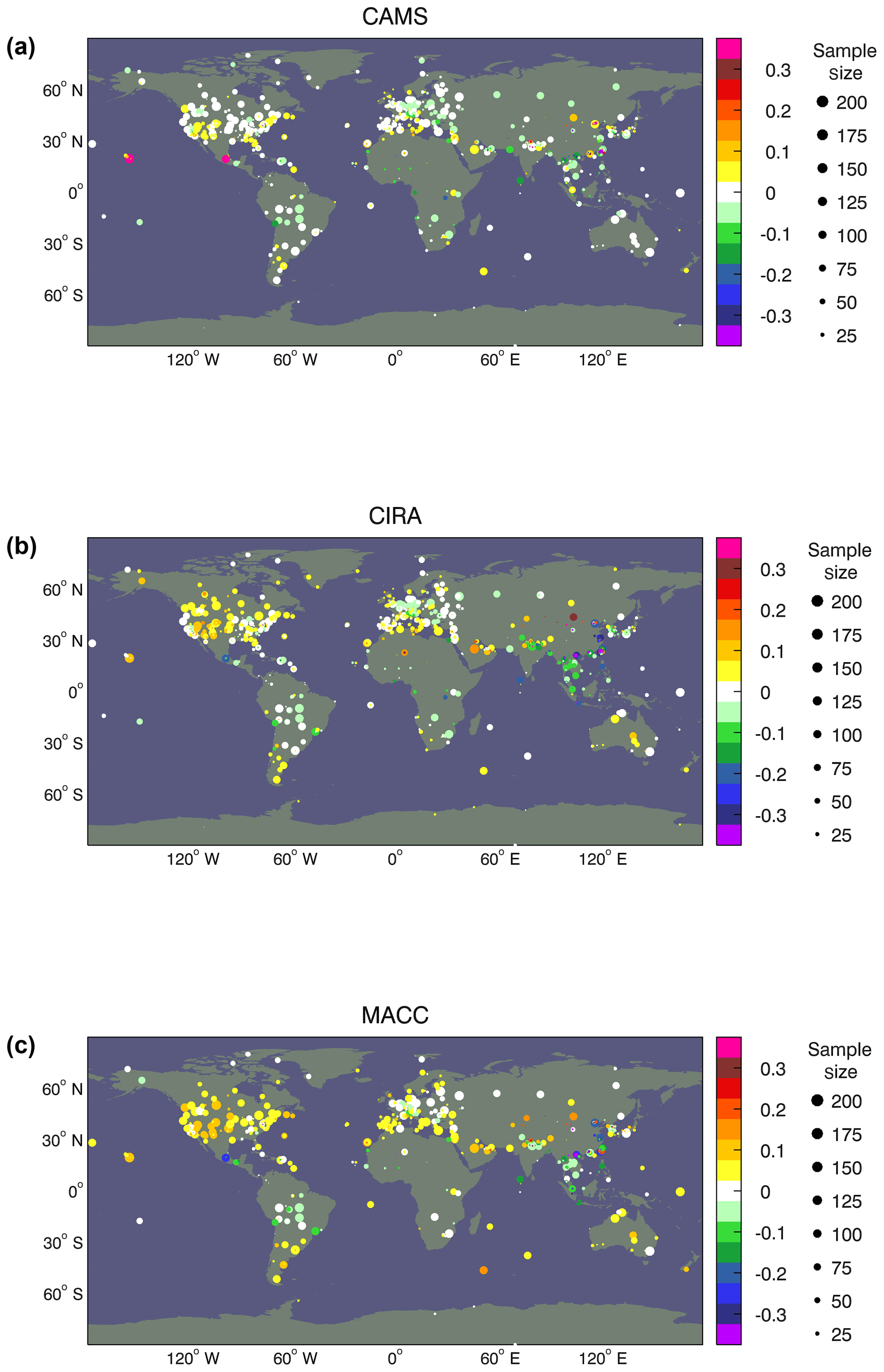
Figure 21Mean Total AOD bias between the three reanalyses and AERONET observations for (a) CAMSRA, (b) CIRA and (c) MACCRA. For CAMSRA and CIRA the average is calculated over the period 2003–2016, and for MACCRA it is calculated only for 2003–2012. AOD is unitless.
The AOD at 550 nm from the reanalyses is evaluated with observations of the AErosol RObotic NETwork (AERONET; Figs. 21–23) Version 3 Level 2.0 data. AERONET is a network of about 400 stations measuring spectral AOD with ground-based sun photometers (Holben et al., 1998). The stations are mostly located over land, with a high number of stations situated in North America and Europe. The global number of stations contributing observations to the evaluation increased from about 60 in 2003 to about 300 in 2016. Figure 21 shows maps of the mean biases from the three reanalyses against AERONET. CAMSRA has the smallest mean bias at most locations, while CIRA shows larger positive biases over North America, Australia and desert areas (North Africa, Middle East and Gobi) and a larger underestimation in India and Southeast Asia. MACCRA has even larger positive biases in North America and larger positive biases in Europe and the Mediterranean. Figure 21 shows that in CAMSRA there are some hotspots around outgassing volcanoes (in particular Mauna Loa and Mexico City) with high analysis AOD values that degrade the global average bias. These hotspots are dominated by sulfate and are a side effect of possibly erroneous model treatment of diffuse volcanic emissions, i.e. the model-resolution orography not resolving the height of the volcanoes and therefore not being representative of the measurement sites with respect to the volcanic plumes. It is also possible that there are errors in how quickly aerosol is formed from diffuse outgassing sources. The volcanic emissions have been unmasked by recent enhancements to the aerosol SO2 oxidation scheme which improve aerosol on the global scale. When calculating global mean statistics, it is advisable to exclude those two stations as unrepresentative.
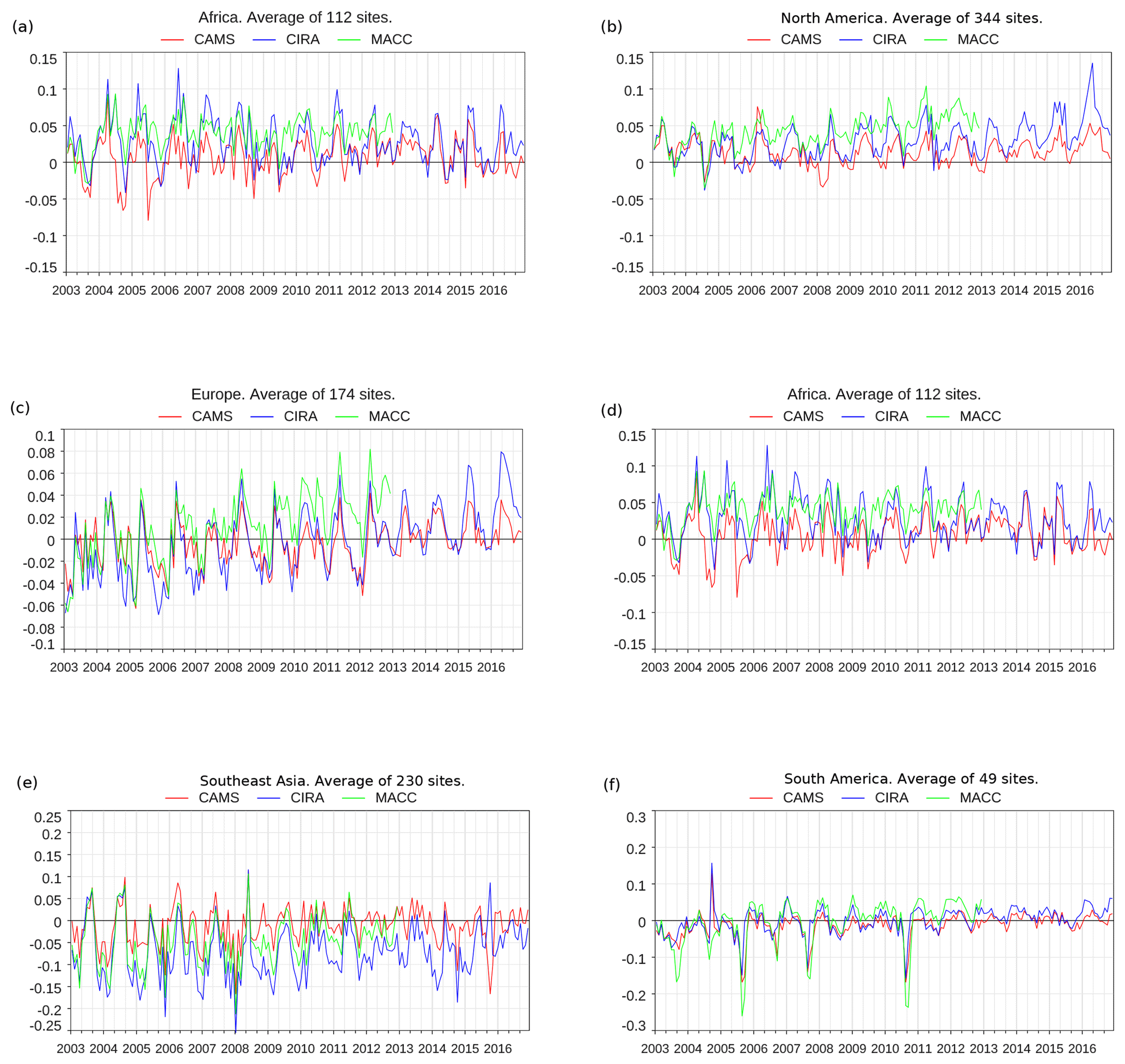
Figure 22Time series of monthly mean bias of total AOD from the reanalyses against AERONET V3 Level 2.0 observations for the following areas: (a) globe, (b) North America, (c) Europe, (d) Africa, (e) Southeast Asia and (f) South America. CAMSRA is shown in red, CIRA in blue and MACCRA in green. Mauna Loa and Mexico City were excluded from these time series, as they are unrepresentative and skew the statistics. AOD is unitless.
Table 8Mean biases and standard deviations from MACCRA, CIRA and CAMSRA relative to AERONET data (shown in Fig. 22). The values are calculated for the period 2003–2012, and the values in brackets are calculated for CIRA and CAMSRA for the period 2003–2016. Numbers in italics mark where MACCRA or CIRA have larger biases or a larger standard deviation than CAMSRA, and the numbers in bold mark where their values are smaller. AOD is unitless.
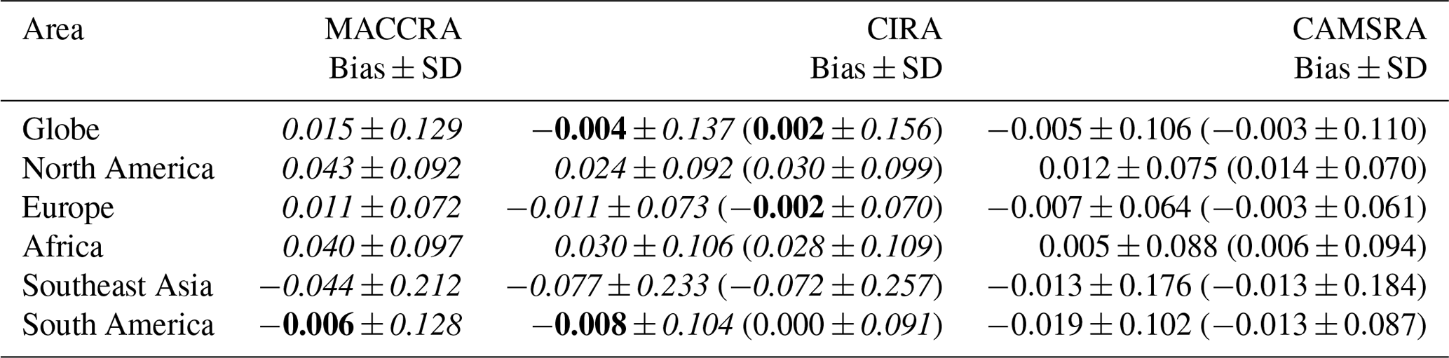
Figure 22 shows time series of monthly mean biases from the three reanalyses against AERONET for several areas, and Table 8 shows the corresponding mean biases and their standard deviations. Figure 23 shows global correlation coefficients with AERONET. As explained above, Mauna Loa and Mexico City were excluded from these statistics. As already seen in Fig. 21, CAMSRA has the smallest bias with respect to the AERONET data in most areas (see also Table 8) and has the largest correlation coefficient (Fig. 23). It shows a good consistency throughout the time period from 2003 to 2016, while MACCRA shows an increasing positive bias with time in Europe and North America. CIRA also shows increasing positive biases with time in North America, particularly from 2013 onwards, and a change in biases in Europe, from negative at the beginning of the time series to positive at the end. It still has to be assessed if this improvement is due to model changes or a better representation of the emissions in CAMSRA. There is a change to slightly higher AOD in CAMSRA (biases more positive in the global mean and in particular over Europe and North America) that seems to coincide with the loss of AATSR data in April 2012. Over Southeast Asia all reanalyses have a negative bias, with CAMSRA having the smallest and CIRA the largest bias (see Table 8). In the NH, the bias changes with season and is largest (positive) during the summer months.
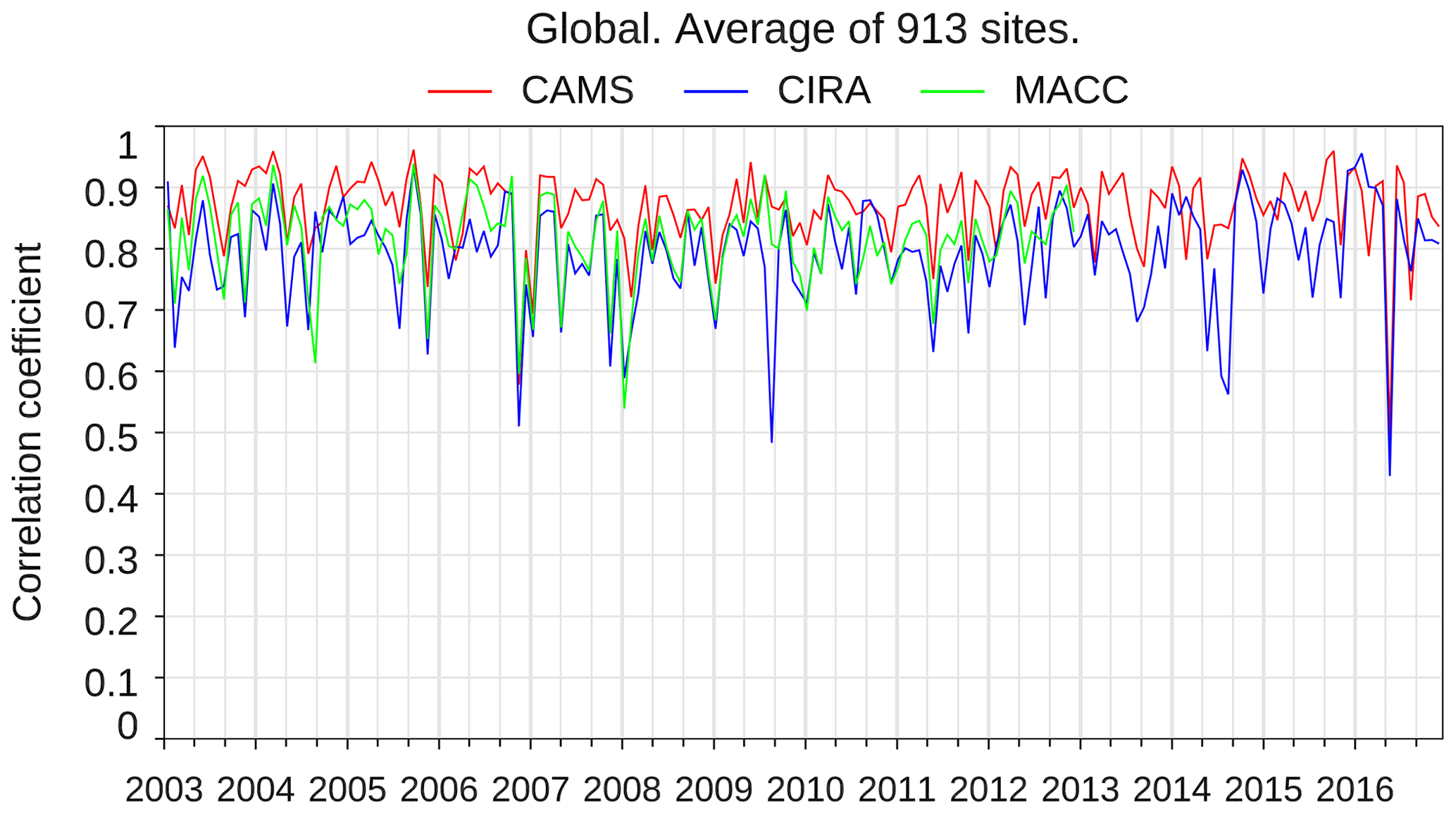
Figure 23Time series of global correlation coefficient with AERONET AOD from the three reanalyses. CAMSRA is shown in red, CIRA in blue and MACCRA in green.
We do not have observations to validate the individual aerosol components, but the simulated aerosol size distribution and implicitly the aerosol composition may be validated to first order by using the wavelength-dependent variation in AOD. It is expressed as Ångström exponent (AE), with higher Ångström exponents indicative of smaller particles and dominance of sulfate and organic aerosols. AE is dependent little on the wavelength itself. We compute it here from AOD at 440 and AOD at 870 nm, except in CIRA, where only AOD at 550 and AOD at 670 nm were available. Figure 24 shows the temporal evolution of simulated and observed mean AE, as well as the correlation. CAMSRA and CIRA show less variability compared with the observations, overestimating mostly the Ångström exponent (5 %–20 %). Overestimation appears mainly in late spring, indicating possibly too little coarse dust. The bias is, however, considerably smaller than for MACCRA, the latter having a significant low bias. Total AOD is composed of less dust in CAMSRA and CIRA compared with MACCRA. This may explain the higher overall Ångström values in CAMSRA. Spatio-temporal correlation in Fig. 24 is higher in winter in the CAMSRA and indicates partially better tracing of aerosol size and implicitly composition variability than in both CIRA and MACCRA.
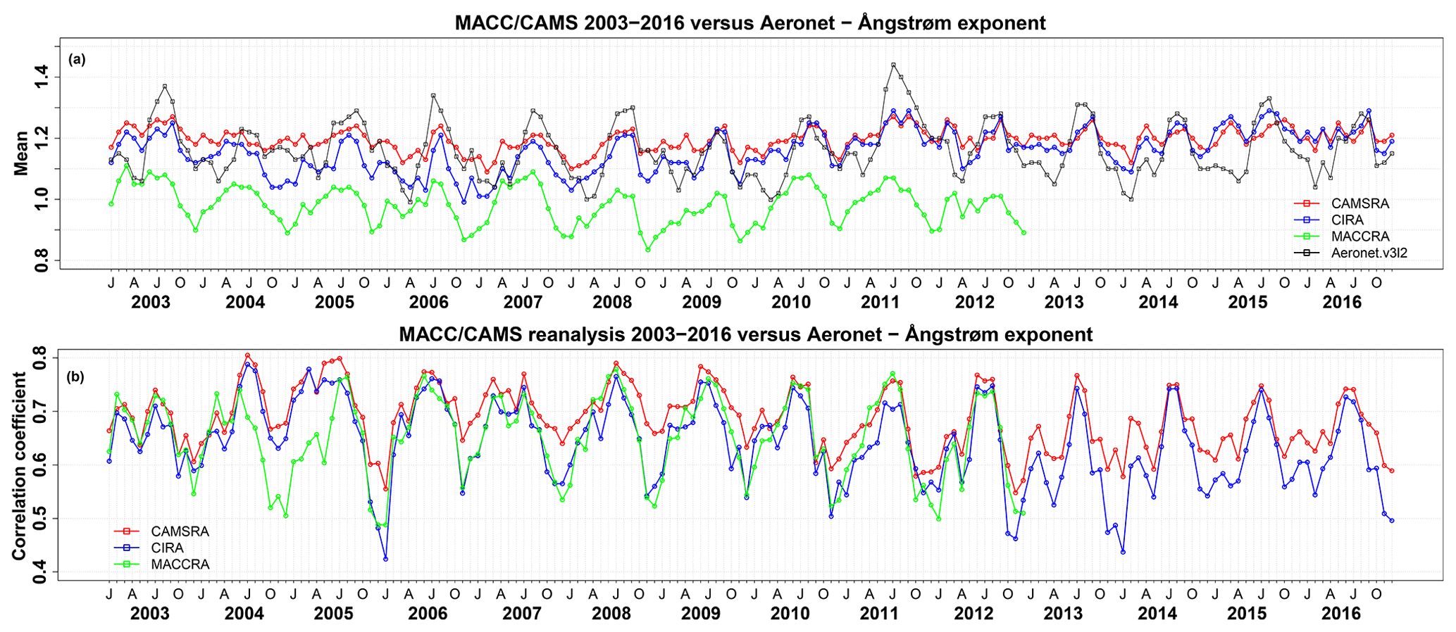
Figure 24Evolution of (a) global mean Ångström exponent at AERONET sites based on matching daily data from model and AERONET, and (b) correlation using daily matching Ångström exponent from model and AERONET. CAMSRA is shown in red, CIRA in blue, MACCRA in green and AERONET Version 3 Level 2.0 observations in black.
In summary, there has been a large change in aerosol composition in CAMSRA compared with the previous reanalysis, making it impossible to compare aerosol species from CAMSRA with climatologies built from CIRA or MACCRA. There is a pronounced reduction in sulfate in CAMSRA, which was too high in CIRA. More work is needed to validate the individual aerosol components against independent observations. CAMSRA total AOD shows reduced biases against AERONET observations and a better temporal consistency, while the older reanalyses show biases that increase with time over North America and Europe. CAMSRA shows AOD values that are too high around outgassing volcanoes (Mauna Loa and Mexico), and we recommend excluding those locations as unrepresentative when calculating global mean statistics.
The Copernicus Atmosphere Monitoring Service (CAMS) has produced a new reanalysis dataset of atmospheric composition, referred to as CAMSRA in this paper. This reanalysis currently covers the years 2003–2016 and will be extended in the future by adding 1 year each year. It was produced by assimilating satellite retrievals of O3, CO, NO2 and AOD from various sensors in ECMWF's Integrated Forecast System (IFS). The new CAMS reanalysis builds on the experience gained during the production of the earlier MACC reanalysis (MACCRA) and CAMS interim reanalysis (CIRA). Great care has been taken to ensure that the emission datasets used in CAMSRA were consistent in time and that consistent anthropogenic, biogenic and biomass burning emissions were used in the aerosol and chemistry modules. Furthermore, a newer (and therefore better) version of the IFS was used, and new, reprocessed datasets for assimilation were acquired as far as possible. Variational bias correction was applied to some of the O3, CO, NO2 and AOD data to ensure good temporal consistency when blending the various datasets. Known problems from earlier reanalyses were avoided, e.g. issues with the bias correction of MLS data in MACCRA that led to drifts in the ozone field, and a better time consistency in the CO field of CAMSRA than of MACCRA was obtained by assimilating data from only one instrument, i.e. MOPITT. CAMSRA therefore shows a more temporally consistent performance than the previous two reanalyses and has mostly smaller biases with respect to independent observations in most areas for O3, CO, NO2 and AOD.
The validation results presented in this paper have shown that mean TCO3 fields from CAMSRA and CIRA are similar and agree to within 1 % when averaged over the period 2003–2016. The differences between CAMSRA and MACCRA are larger but are still within 5 %. All reanalyses have small positive biases with respect to Dobson TCO3 observations, with MACCRA having the largest global mean bias and CAMSRA the smallest (see Table 3). Agreement with ozone-sondes is within 10 % in the long-term global mean. The reanalyses agree well in the stratosphere and have larger differences in the troposphere. CAMSRA agrees better with ozone-sondes above 15 hPa than MACCRA, which overestimates O3 there. This makes CAMSRA a better dataset to be used as climatology in, for example, radiation schemes or radiance observation operators. CAMSRA and CIRA agree better with ozone-sondes in the tropical mid-troposphere to upper troposphere than MACCRA, which shows a large underestimation here (−30 %). O3 from CAMSRA is more consistent in time than MACCRA because the variational bias correction applied to MLS O3 retrievals during some of MACCRA led to drifts in the O3 field, particularly noticeable in the troposphere in MACCRA (Inness et al., 2013). CAMSRA shows a smaller underestimation of surface O3 in the NH during boreal spring than the previous reanalyses. We note that there is an increased seasonally varying tropospheric ozone bias in CAMSRA after 2013, particularly in the Antarctic and Arctic. The reason for this bias is still being investigated, and the same bias is also found in the CAMS real-time ozone analysis. There are larger ozone biases in all three reanalyses between March and August 2004 when no O3 profile data were available for assimilation than during the rest of the period, and there are larger biases during 2003, when MIPAS and SCIAMACHY O3 data of poorer quality were assimilated.
For CO, CAMSRA shows good agreement with TCCON observations, with small biases and a good representation of the seasonal cycle and inter-annual variability. CAMSRA has the smallest bias out of the three reanalyses with respect to most of the TCCON stations looked at in this paper, with a small negative bias in the NH and a small positive bias in the tropics and SH (Table 5). Especially in the tropics and SH the biases in CAMSRA are reduced much compared with CIRA and MACCRA. Comparisons with IAGOS aircraft data show an underestimation of CO in the free troposphere in the NH (< 10 %) with larger underestimation in the lower troposphere. This underestimation is similar in CAMSRA and CIRA, while MACCRA has larger negative biases in the NH lower troposphere. CAMSRA also has smaller biases with respect to GAW surface CO than MACCRA over Europe and North America, but surface CO values are overestimated over Indonesia in CAMSRA, leading to larger global mean CO biases relative to GAW (Table 6). The choice of fire emissions has a large impact on the TCCO field, and the largest differences between CAMSRA and MACCRA are seen in biomass burning areas because different fire emission datasets were used in these reanalyses. CO from CAMSRA is more consistent in time than MACCRA, which showed some changes in the CO field because the assimilation of IASI CO was started in MACCRA in 2008 (Inness et al., 2013), while in CAMSRA and CIRA only TCCO from MOPITT was assimilated.
For NO2, data from more instruments were assimilated in CAMSRA (SCIAMACHMY, OMI and GOME-2) than in CIRA (none) and MACCRA (SCIAMACHY only). This led to differences between the reanalyses, but the limited amount of independent validation observations for NO2 made it difficult to assess these differences. The seasonal cycle of the tropospheric NO2 columns is underestimated over East Asia, and to a smaller extent, over Europe by all three reanalyses compared with a tropospheric column NO2 dataset based on SCIAMACHY and GOME-2A data. CAMSRA shows the smallest bias out of the three reanalyses over East Asia, suggesting that the assimilation of several NO2 satellite retrievals improves the NO2 analysis. However, the comparison also showed that the quality of the NO2 analysis in CAMSRA was degraded during 2003 because of the reduced quality of the assimilated SCHIAMACHY NO2 data (Fig. S5a) during that time. Compared with European GAW NO2 surface observations, the reanalyses reproduced the observed mean values and the seasonal variability well but again showed an underestimation of high wintertime values. CAMSRA generally had the smallest biases (Table 7). More work is needed to validate the NO2 fields from CAMSRA thoroughly and to assess if the wintertime underestimation is due to shortcomings of the model or the emissions.
Total AOD values in CAMSRA are reduced compared with CIRA and MACCRA in many areas but increased over India and Southeast Asia and agree better with AERONET total AOD with reduced biases in most areas (Table 8). AOD in CAMSRA is more consistent in time than in CIRA and MACCRA, especially over Europe and North America, where CIRA and MACCRA show an increasingly positive bias with time. There are large differences in aerosol speciation (which is less constrained by the assimilated AOD observations) between CAMSRA, CIRA and MACCRA. Relative to both the earlier reanalyses, CAMSRA shows a reduction in desert dust, sulfates and black carbon in the SH, compensated by an increase in organic matter and black carbon in the NH. The reduction in sulfate globally is particularly strong relative to CIRA, where its contribution was overestimated (Flemming et al., 2017b), suggesting that this is a clear improvement in CAMSRA. CAMSRA shares the lower sea salt of CIRA in the SH but is closer to the higher values of MACCRA in the NH. The larger role played by organic matter in CAMSRA reflects the inclusion of a proxy for anthropogenic SOA added to organic matter, which was missing from the earlier reanalyses. Time series and correlation of the Ångström exponent indicate partially better tracing of aerosol size and implicitly of composition variability of CAMSRA than in both CIRA and MACCRA. Validation of AOD with AERONET data shows there are some hotspots around outgassing volcanoes (in particular Mauna Loa and Mexico City) with high analysis AOD values in CAMSRA that degrade the global average bias. This is a side effect of possibly erroneous model treatment of diffuse volcanic emissions, i.e. the model-resolution orography not resolving the height of the volcanoes and therefore not being representative of the measurement sites with respect to the volcanic plumes. When calculating global mean statistics, it is advisable to exclude these two stations as unrepresentative.
In addition to being a dataset of better quality and better temporal consistency, CAMSRA has the advantage that it provides more chemical species than CIRA (where only a limited subset was archived) and that data are available at a higher temporal and spatial resolution. In total 56 tropospheric chemical species of the CB05 chemical mechanism, 12 aerosol components and many additional diagnostics such as total columns and extinction coefficients can be obtained from CAMSRA. An inventory of the available model fields can be found at http://apps.ecmwf.int/data-catalogues/cams-reanalysis/?class=mc&expver=eac4 (last access: 15 March 2019). Users who previously used the MACCRA or CIRA data should note that because of the differences seen between CAMSRA and the older reanalyses, it is not advisable to concatenate data from the older reanalyses with CAMSRA data from more recent years but also that CAMSRA data should be used for the whole period of interest.
The CAMSRA data are freely available (http://atmosphere.copernicus.eu/copernicus-releases-new-global-reanalysis-data-set-atmospheric-composition, last access: 15 March 2019) and will become available from the Copernicus Atmosphere Data Store. The data can serve a multitude of users, from application developers to scientists and policymakers. They can be used to analyse the state of the atmosphere or to look at trends that have developed over the past years or decades. Furthermore, the CAMS reanalysis can be used to compute climatologies, evaluate models, benchmark other reanalyses or serve as boundary conditions for regional models for past periods.
One limitation of CAMSRA is that it does not use a stratospheric chemistry scheme (apart form a Cariolle-type parametrisation for stratospheric ozone), and the stratospheric concentrations apart from ozone need to be considered with caution. For any future reanalysis, we plan to implement a full stratospheric chemistry scheme and to increase the vertical resolution to bring it into line with the vertical resolution used in ECMWF's NWP system (currently 137 levels, model top at 0.01 hPa). It might also be beneficial to include the chemistry in the adjoint and tangent linear model of the IFS and to recalculate the background error statistics for the atmospheric composition variables with the latest version of the model. More time should be spent on acquiring and assessing new observations so that problems like the OMI row anomaly are addressed properly and the quality of the reanalysis is not degraded at times when lower quality data are assimilated (e.g. degraded NO2 analysis during 2003 because of worse-quality SCIAMACHY data). It would also be advisable to explore the use of reprocessed datasets thoroughly, e.g. datasets processed by ESA's Climate Change Initiative (CCI) and the Seventh Framework Programme (FP7) Quality Assurance for Essential Climate Variables (QA4ECV) project. It could also be investigated if enough atmospheric composition datasets are available prior to 2003 to start a future reanalysis before 2003. Furthermore, work has started to look at emission inversion with the CAMS system, and we hope the next reanalysis will include some inversion capability to update the emissions during the assimilation according to the satellite observations.
The CAMS reanalysis data are freely available from https://atmosphere.copernicus.eu/ (last access: 18 March 2019) and will become available via the Copernicus Atmosphere Data Store shortly.
Table A1List of GEMS–MACC–CAMS model versions showing the time evolution of the real-time CAMS system since July 2008.
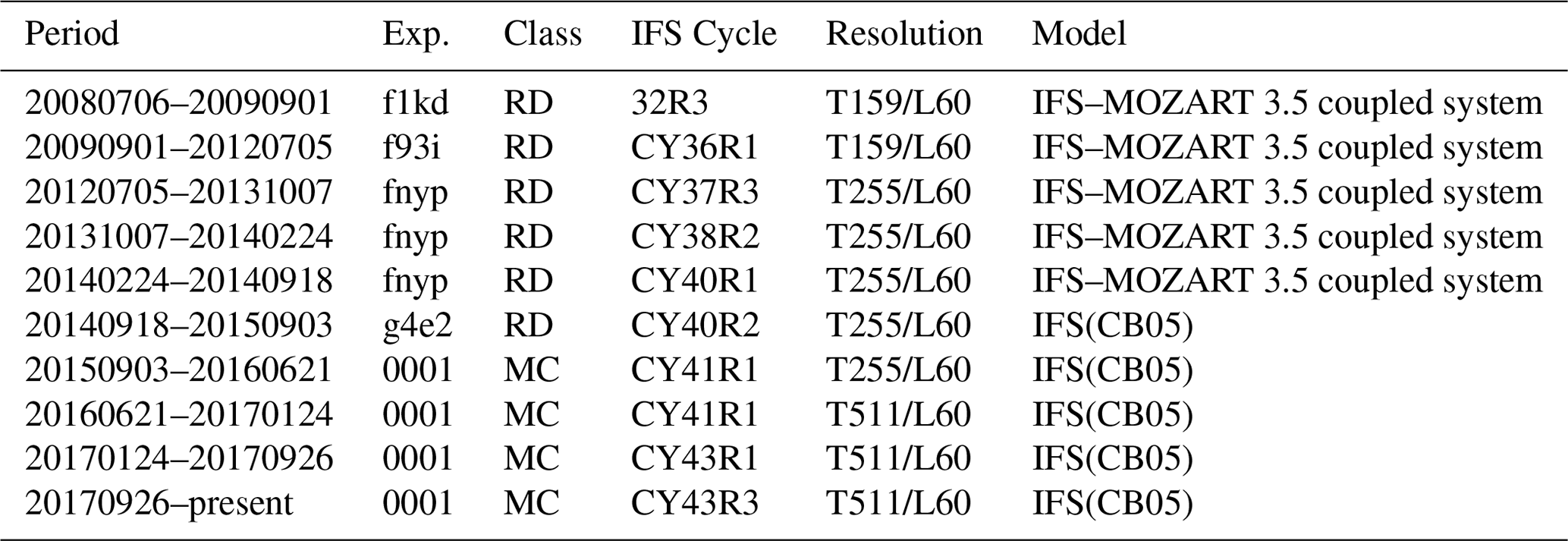
Table A2Reanalyses of atmospheric composition produced with the GEMS–MACC–CAMS system.
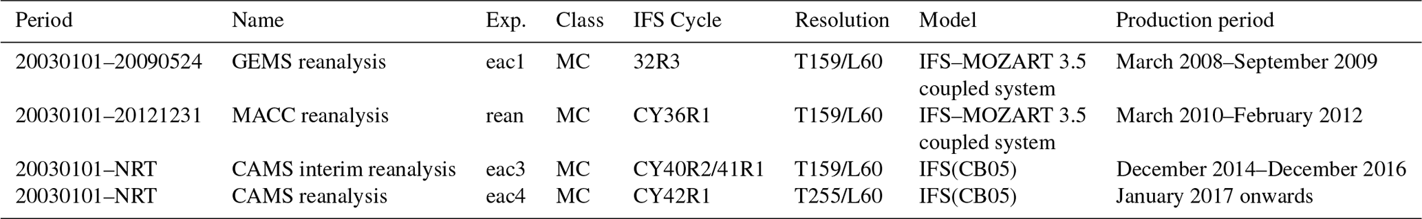
The Figure of Merit in space (FMS; Chang and Hanna, 2004) score compares the fit of the model ozone profiles to observation profiles (e.g. ozone-sondes) given in partial pressure (millipascal), has a score between 1 (perfect fit) and 0 and is defined as
where M is the model profile, O is the observation profile, and ptop and pbot are the top and bottom pressure values of the layer considered, respectively. For Fig. 1 we used ptop=3 hPa and pbot=1000 hPa.
The modified normalised mean bias (MNMB) is defined as
with N as the number of observations, m as the model and o the observed values.
We summarise some issues here that might affect the quality of the CAMS reanalysis which were known at the time of publication. This list is also available from https://confluence.ecmwf.int/display/CKB/CAMS+Reanalysis+data+documentation (last access: 15 March 2019), where it will be maintained and updated.
C1 Ozone
-
2003. There is degraded quality (bigger biases with respect to observations) in Arctic and Antarctic free troposphere because MIPAS and SCIAMACHY data of poorer quality were assimilated.
-
March–August 2004. No profile data were available for the assimilation. This affects the vertical structure of the ozone analysis, and we see larger biases compared with ozone-sondes.
-
2013–2016. Larger seasonally varying biases are present from 2013 onwards in the free troposphere, particularly in the Arctic and Antarctic. This must be due to a change in the observing system and is still under investigation. It is also found in the CAMS NRT analyses.
-
Technical comment. CAMS data users should use the GEMS Ozone (grib parameter 210203) and Total Column GEMS Ozone (grib parameter 210206) fields. These are produced specifically for CAMS using the full tropospheric chemistry scheme and are the fields described in this paper.
C2 CO
-
CAMSRA has larger surface CO values than the other two reanalyses over Indonesia, especially during years with high biomass burning activity, leading to increased overestimation relative to GAW CO surface observations.
NO2
-
During 2003 the seasonal cycle of tropospheric NO2 is not well represented because of assimilating SCIAMACHY NO2 retrievals of poorer quality.
C4 AOD
-
Validation of AOD with AERONET data has shown that there are some hotspots around outgassing volcanoes (in particular Mauna Loa and Mexico City), with high analysis AOD values that degrade the global average bias. When calculating global mean statistics, it is advisable to exclude those two stations as unrepresentative. This is a side effect of model-resolution orography not resolving the height of the volcanoes that has been unmasked by recent enhancements to the SO2 oxidation scheme which improve aerosol on the global scale.
-
There is a change to slightly higher AOD in CAMSRA (biases more positive in the global mean and in particular over Europe and North America) that seems to coincide with the loss of AATSR data in April 2012.
The supplement related to this article is available online at: https://doi.org/10.5194/acp-19-3515-2019-supplement.
AI prepared the data assimilation of the chemistry fields, ran the reanalysis experiments, carried out a lot of the validation and wrote the paper. MA contributed to the assimilation of aerosol data and produced the AERONET, GAW and WOUDC validation plots; AAP and SM provided the code for the TCCON validation and Fig. 13; JB and SM helped with the assimilation of the reactive gases and greenhouse gases; AB and MS provided Fig. 24 and the corresponding text; AMB provided Fig. 18; JD, MR and MS helped with the acquisition of the data that were assimilated in the CAMS reanalysis, re-archiving of the CAMS reanalysis experiments and data provision to users; RE and VHP provided useful feedback on the paper and help in the coordination of the reanalysis; HE coordinated the CAMS_84 validation activities and provided feedback on the paper; JF and VH worked on the chemistry scheme of the IFS and JF provided Figs. 2, 3, 7, 12, 17 and 20; LJ provided the software for the validation with ozone-sondes as well as GAW, WOUDC, AERONET and IAGOS data and helped with the figures using those data; ZK and SR worked on the aerosol model and aerosol validation; and MP worked on the emissions and provided Fig. 4.
The authors declare that they have no conflict of interest.
Thanks to the data providers of the data assimilated in the CAMS reanalysis and the data used for the validation studies in this paper. The Copernicus Atmosphere Monitoring Service is operated by the European Centre for Medium-Range Weather Forecasts on behalf of the European Commission as part of the Copernicus Programme (http://copernicus.eu, last access: 15 March 2019).
This paper was edited by Kostas Tsigaridis and reviewed by two anonymous referees.
Agustí-Panareda, A., Massart, S., Chevallier, F., Boussetta, S., Balsamo, G., Beljaars, A., Ciais, P., Deutscher, N. M., Engelen, R., Jones, L., Kivi, R., Paris, J.-D., Peuch, V.-H., Sherlock, V., Vermeulen, A. T., Wennberg, P. O., and Wunch, D.: Forecasting global atmospheric CO2, Atmos. Chem. Phys., 14, 11959–11983, https://doi.org/10.5194/acp-14-11959-2014, 2014.
Barré, J., Gaubert, B., Arellano, A. F. J., Worden, H. M., Edwards, D. P., Deeter, M. N., Anderson, J. L., Raeder, K., Collins, N., and Tilmes, S.: Assessing the impacts of assimilating IASI and MOPITT CO retrievals using CESM-CAM-chem and DART, J. Geophys. Res.-Atmos., 120, 10501–10529, https://doi.org/10.1002/2015JD023467, 2015.
Basher, R. E.: Review of the Dobson spectrophotometer and its accuracy, Global Ozone Res. Monit. Proj., Rep. 13, World Meteor. Organ., Geneva, Switzerland, December, available at: http://www.esrl.noaa.gov/gmd/ozwv/dobson/papers/report13/report13.html (last access: 3 February 2017), 1982.
Benedetti, A. and Fisher M.: Background error statistics for aerosols, Q. J. Roy. Meteor. Soc., 133, 391–405, 2007.
Benedetti, A., Morcrette, J.-J., Boucher, O., Dethof, A., Engelen, R. J., Fisher, M., Flentje, H., Huneeus, N., Jones, L., Kaiser, J. W., Kinne, S., Mangold, A., Razinger, M., Simmons, A. J., Suttie, M., and the GEMS-AER team: Aerosol analysis and forecast in the European Centre for Medium-Range Weather Forecasts Integrated Forecast System: Data Assimilation. J. Geophys. Res., 114, D13205, https://doi.org/10.1029/2008JD011115, 2009.
Bhartia, P. K., McPeters, R. D., Mateer, C. L., Flynn, L. E., and Wellemeyer, C., Algorithm for the estimation of vertical ozone profiles from the backscattered ultraviolet technique, J. Geophys. Res., 101, 18793–18806, 1996.
Blumenstock, T., Hase, F., Schneider, M., García, O. E., and Sepílveda, E.: TCCON data from Izaña, Tenerife, Spain, Release GGG2014R1, TCCON data archive, hosted by CaltechDATA, California Institute of Technology, Pasadena, CA, USA, https://doi.org/10.14291/tccon.ggg2014.izana01.R1, 2017.
Boersma, K. F., Eskes, H. J., and Brinksma, E. J.: Error analysis for tropospheric NO2 retrieval from space, J. Geophys. Res., 109, D04311, https://doi.org/10.1029/2003JD003962, 2004.
Boersma, K. F., Eskes, H. J., Veefkind, J. P., Brinksma, E. J., van der A, R. J., Sneep, M., van den Oord, G. H. J., Levelt, P. F., Stammes, P., Gleason, J. F., and Bucsela, E. J.: Near-real time retrieval of tropospheric NO2 from OMI, Atmos. Chem. Phys., 7, 2103–2118, https://doi.org/10.5194/acp-7-2103-2007, 2007.
Boersma, K. F., Eskes, H. J., Dirksen, R. J., van der A, R. J., Veefkind, J. P., Stammes, P., Huijnen, V., Kleipool, Q. L., Sneep, M., Claas, J., Leitão, J., Richter, A., Zhou, Y., and Brunner, D.: An improved tropospheric NO2 column retrieval algorithm for the Ozone Monitoring Instrument, Atmos. Meas. Tech., 4, 1905–1928, https://doi.org/10.5194/amt-4-1905-2011, 2011.
Bozzo, A., Remy, S., Benedetti, A., Flemming, J., Bechtold, P., Rodwell, M., and Morcrette, J. J.: Implementation of a CAMS-based aerosol climatology in the IFS. ECMWF Technical Memorandum 801, available at: https://www.ecmwf.int/en/elibrary/17771-radiation-numerical-weather-prediction (last access: 15 March 2019), 2017.
Buchard, V., da Silva, A. M., Colarco, P. R., Darmenov, A., Randles, C. A., Govindaraju, R., Torres, O., Campbell, J., and Spurr, R.: Using the OMI aerosol index and absorption aerosol optical depth to evaluate the NASA MERRA Aerosol Reanalysis, Atmos. Chem. Phys., 15, 5743–5760, https://doi.org/10.5194/acp-15-5743-2015, 2015.
Buchard, V., Randles, C. A., da Silva, A. M., Darmenov, A., Colarco, P. R., Govindaraju, R., Ferrare, R., Hair, J., Beyersdorf, A. J., Ziemba, L. D., and Yu, H.: The MERRA-2 Aerosol Reanalysis, 1980 Onward. Part II: Evaluation and Case Studies, J. Climate, 30, 6851–6872, https://doi.org/10.1175/JCLI-D-16-0613.1, 2017.
Cariolle, D. and Déqué, M.: Southern hemisphere medium-scale waves and total ozone disturbances in a spectral general circulation model, J. Geophys. Res., 91, 10825–10846, 1986.
Cariolle, D. and Teyssèdre, H.: A revised linear ozone photochemistry parameterization for use in transport and general circulation models: multi-annual simulations, Atmos. Chem. Phys., 7, 2183–2196, https://doi.org/10.5194/acp-7-2183-2007, 2007.
Chang, J. and Hanna, S.: Air quality model performance evaluation, Meteorol. Atmos. Phys., 87, 167–196, https://doi.org/10.1007/s00703-003-0070-7, 2004.
Clerbaux, C., Boynard, A., Clarisse, L., George, M., Hadji-Lazaro, J., Herbin, H., Hurtmans, D., Pommier, M., Razavi, A., Turquety, S., Wespes, C., and Coheur, P.-F.: Monitoring of atmospheric composition using the thermal infrared IASI/MetOp sounder, Atmos. Chem. Phys., 9, 6041–6054, https://doi.org/10.5194/acp-9-6041-2009, 2009.
Courtier, P., Thépaut, J.-N., and Hollingsworth, A.: A strategy for operational implementation of 4D-Var, using an incremental approach, Q. J. Roy. Meteor. Soc., 120, 1367–1388, 1994.
Dee, D. P. and Uppala, S.: Variational bias correction of satellite radiance data in the ERA-Interim reanalysis, Q. J. Roy. Meteor. Soc., 135, 1830–1841, 2009.
Dee, D. P., Uppala, S. M., Simmons, A. J., Berrisford, P., Poli, P., Kobayashi, S., Andrae, U., Balmaseda, M. A., Balsamo, G., Bauer, P., Bechtold, P., Beljaars, A. C. M., van de Berg, L., Bidlot, J., Bormann, N., Delsol, C., Dragani, R., Fuentes, M., Geer, A. J., Haimberger, L., Healy, S. B., Hersbach, H., Hólm, E. V., Isaksen, L., Kållberg, P., Köhler, M., Matricardi, M., McNally, A. P., Monge-Sanz, B. M., Morcrette, J.-J., Park, B.-K., Peubey, C., de Rosnay, P., Tavolato, C., Thépaut, J.-N., and Vitarta, F.: The ERA-Interim reanalysis: Configuration and performance of the data assimilation system, Q. J. Roy. Meteor. Soc., 137, 553–597, 2011.
Deeter, M. N., Martínez-Alonso, S., Edwards, D. P., Emmons, L. K., Gille, J. C., Worden, H. M., Pittman, J. V., Daube, B. C., and Wofsy, S. C.: Validation of MOPITT Version 5 thermal-infrared, near-infrared, and multispectral carbon monoxide profile retrievals for 2000–2011, J. Geophys. Res.-Atmos., 118, 6710–6725, https://doi.org/10.1002/jgrd.50272, 2013.
Deeter, M. N., Martínez-Alonso, S., Edwards, D. P., Emmons, L. K., Gille, J. C., Worden, H. M., Sweeney, C., Pittman, J. V., Daube, B. C., and Wofsy, S. C.: The MOPITT Version 6 product: algorithm enhancements and validation, Atmos. Meas. Tech., 7, 3623–3632, https://doi.org/10.5194/amt-7-3623-2014, 2014.
Diamantakis, M. and Flemming, J.: Global mass fixer algorithms for conservative tracer transport in the ECMWF model, Geosci. Model Dev., 7, 965–979, https://doi.org/10.5194/gmd-7-965-2014, 2014.
Ding, J., Miyazaki, K., van der A, R. J., Mijling, B., Kurokawa, J.-I., Cho, S., Janssens-Maenhout, G., Zhang, Q., Liu, F., and Levelt, P. F.: Intercomparison of NOx emission inventories over East Asia, Atmos. Chem. Phys., 17, 10125–10141, https://doi.org/10.5194/acp-17-10125-2017, 2017.
Eskes, H. J., Bennouna, Y. Schulz, M., Christophe, Y., Basart, S., Benedictow, A., Blechschmidt, A.-M., Chabrillat, S., Clark, H., Cuevas, E., Flentje, H., Hansen, K. M., Im, U., Kapsomenakis, J., Langerock, B., Petersen, K., Richter, A., Sudarc Hikova, N., Thouret, V., Wagner, A., Wang, Y., and Zeferos, C.: Copernicus Atmosphere Monitoring Service (CAMS) report, CAMS84_2015SC2_D84.7.1.4_Y14_v1.pdf, available at: https://atmosphere.copernicus.eu/sites/default/files/2018-09/CAMS84_2015SC2_D84.7.1.4_Y14_v1.pdf (last access: 15 March 2019), 2018.
Flemming, J. and Inness, A.: Carbon Monoxide [in “State of the Climate in 2017”], B. Am. Meteorol. Soc., 99, S59–S61, 2018.
Flemming, J., Inness, A., Flentje, H., Huijnen, V., Moinat, P., Schultz, M. G., and Stein, O.: Coupling global chemistry transport models to ECMWF's integrated forecast system, Geosci. Model Dev., 2, 253–265, https://doi.org/10.5194/gmd-2-253-2009, 2009.
Flemming, J., Inness, A., Jones, L., Eskes, H. J., Huijnen, V., Schultz, M. G., Stein, O., Cariolle, D., Kinnison, D., and Brasseur, G.: Forecasts and assimilation experiments of the Antarctic ozone hole 2008, Atmos. Chem. Phys., 11, 1961–1977, https://doi.org/10.5194/acp-11-1961-2011, 2011.
Flemming, J., Huijnen, V., Arteta, J., Bechtold, P., Beljaars, A., Blechschmidt, A.-M., Diamantakis, M., Engelen, R. J., Gaudel, A., Inness, A., Jones, L., Josse, B., Katragkou, E., Marecal, V., Peuch, V.-H., Richter, A., Schultz, M. G., Stein, O., and Tsikerdekis, A.: Tropospheric chemistry in the Integrated Forecasting System of ECMWF, Geosci. Model Dev., 8, 975–1003, https://doi.org/10.5194/gmd-8-975-2015, 2015.
Flemming, J., Peuch, V.-H., and Jones, L.: Ten years of forecasting atmospheric composition at ECMWF, ECMWF newsletter 152, available at: https://www.ecmwf.int/en/newsletter/152/news/ten-years-forecasting-atmospheric-composition-ecmwf (last access: 15 March 2019), 2017a.
Flemming, J., Benedetti, A., Inness, A., Engelen, R. J., Jones, L., Huijnen, V., Remy, S., Parrington, M., Suttie, M., Bozzo, A., Peuch, V.-H., Akritidis, D., and Katragkou, E.: The CAMS interim Reanalysis of Carbon Monoxide, Ozone and Aerosol for 2003–2015, Atmos. Chem. Phys., 17, 1945–1983, https://doi.org/10.5194/acp-17-1945-2017, 2017b.
Gelaro, R., McCarty, W., Suârez, M. J., Todling, R., Molod, A., Takacs, L., Randles, C. A., Darmenov, A., Bosilovich, M. G., Reichle, R., and Wargan, K.: The Modern-Era Retrospective Analysis for Research and Applications, Version 2 (MERRA-2), J. Climate, 30, 5419–5454, https://doi.org/10.1175/JCLI-D-16-0758.1, 2017.
George, M., Clerbaux, C., Hurtmans, D., Turquety, S., Coheur, P.-F., Pommier, M., Hadji-Lazaro, J., Edwards, D. P., Worden, H., Luo, M., Rinsland, C., and McMillan, W.: Carbon monoxide distributions from the IASI/METOP mission: evaluation with other space-borne remote sensors, Atmos. Chem. Phys., 9, 8317–8330, https://doi.org/10.5194/acp-9-8317-2009, 2009.
Ginoux, P., Chin, M., Tegen, I., Prospero, J. M., Holben, B., Dubovik, O., and Lin, S. J.: Sources and distributions of dust aerosols simulated with the GOCART model, J. Geophys. Res., 106, 20255–20273, 2001.
Granier, C., Guenther, A., Lamarque, J. F., Mieville, A., Muller, J. F., Olivier, J., Orlando, J., Peters, J., Petron, G., Tyndall, G., and Wallens, S.: POET, a database of surface emissions of ozone precursors, available at: http://www.aero.jussieu.fr/projet/ACCENT/POET.php (last access: 15 March 2019), 2005.
Granier, C., Bessagnet, B., Bond, T., D'Angiola, A., Denier van der Gon, H., Frost, G. J., Heil, A., Kaiser, J. W., Kinne, S., Klimont, Z., Kloster, S., Lamarque, J.-F., Liousse, C., Masui, T., Meleux, F., Mieville, A., Ohara, R., Raut, J.-C., Riahi, K., Schultz, M. G., Smith, S. G., Thompson, A., van Aardenne, J., van der Werf, G. R., and van Vuuren, D. P.: Evolution of anthropogenic and biomass burning emissions of air pollutants at global and regional scales during the 1980–2010 period, Climatic Change, 109, 163–190, https://doi.org/10.1007/s10584-011-0154-1, 2011.
Griffith, D. W. T., Deutscher, N., Velazco, V. A., Wennberg, P. O., Yavin, Y., Keppel Aleks, G., Washenfelder, R., Toon, G. C., Blavier, J.-F., Murphy, C., Jones, N., Kettlewell, G., Connor, B., Macatangay, R., Roehl, C., Ryczek, M., Glowacki, J., Culgan, T., and Bryant, G.: TCCON data from Darwin, Australia, Release GGG2014R0, TCCON data archive, hosted by CaltechDATA,California Institute of Technology, Pasadena, CA, USA, https://doi.org/10.14291/tccon.ggg2014.darwin01.R0/1149290, 2014.
Guenther, A., Karl, T., Harley, P., Wiedinmyer, C., Palmer, P. I., and Geron, C.: Estimates of global terrestrial isoprene emissions using MEGAN (Model of Emissions of Gases and Aerosols from Nature), Atmos. Chem. Phys., 6, 3181–3210, https://doi.org/10.5194/acp-6-3181-2006, 2006.
Hao, N., Koukouli, M. E., Inness, A., Valks, P., Loyola, D. G., Zimmer, W., Balis, D. S., Zyrichidou, I., Van Roozendael, M., Lerot, C., and Spurr, R. J. D.: GOME-2 total ozone columns from MetOp-A/MetOp-B and assimilation in the MACC system, Atmos. Meas. Tech., 7, 2937–2951, https://doi.org/10.5194/amt-7-2937-2014, 2014.
Hersbach, H., de Rosnay, P., Bell, B., Schepers, D., Simmons, A., Soci, C., Abdalla, S., Alonso-Balmaseda, M., Balsamo, G., Bechtold, P., Berrisford, P., Bidlot, J.-R., de Boisséson, E., Bonavita, M., Browne, P., Buizza, R., Dahlgren, P., Dee, D., Dragani, R., Diamantakis, M., Flemming, J., Forbes, R., Geer, A. J., Haiden, T., Hólm, E., Haimberger, L., Hogan, R., Horányi, A., Janiskova, M., Laloyaux, P., Lopez, P., Munoz-Sabater, J., Peubey, C., Radu, R., Richardson, D., Thépaut, J.-N., Vitart, F., Yang, X., Zsótér, E., and Zuo, H.: Operational global reanalysis: progress, future directions and synergies with NWP, ERA Report Series, Number 27, available at: https://www.ecmwf.int/node/18765 (last access: 15 March 2019), 2018.
Holben, B. N., Eck, T. F., Slutsker, I., Tanré, D., Buis, J. P., Setzer, A., Vermote, E., Reagan, J. A., Kaufman, Y., Nakajima, T., Lavenu, F., Jankowiak, I., and Smirnov, A.: AERONET – A federated instrument network and data archive for aerosol characterization, Remote Sens. Environ., 66, 1–16, 1998.
Hollingsworth, A., Engelen, R. J., Textor, C., Benedetti, A., Boucher, O., Chevallier, F., Dethof, A., Elbern, H., Eskes, H., Flemming, J., Granier, C., Kaiser, J. W., Morcrette, J.-J., Rayner, R., Peuch, V.-H., Rouil, L., Schultz, M. G., Simmons, A. J., and The GEMS Consortium: Toward a Monitoring and Forecasting System For Atmospheric Composition: The GEMS Project, B. Am. Meteorol. Soc., 89, 1147–1164, https://doi.org/10.1175/2008BAMS2355.1, 2008.
Huijnen, V., Williams, J. E., and Flemming, J.: Modeling global impacts of heterogeneous loss of HO2 on cloud droplets, ice particles and aerosols, Atmos. Chem. Phys. Discuss., 14, 8575–8632, https://doi.org/10.5194/acpd-14-8575-2014, 2014.
Huijnen, V., Williams, J., van Weele, M., van Noije, T., Krol, M., Dentener, F., Segers, A., Houweling, S., Peters, W., de Laat, J., Boersma, F., Bergamaschi, P., van Velthoven, P., Le Sager, P., Eskes, H., Alkemade, F., Scheele, R., Nédélec, P., and Pätz, H.-W.: The global chemistry transport model TM5: description and evaluation of the tropospheric chemistry version 3.0, Geosci. Model Dev., 3, 445–473, https://doi.org/10.5194/gmd-3-445-2010, 2010.
Huijnen, V., Wooster, M. J., Kaiser, J. W., Gaveau, D. L. A., Flemming, J., Parrington, M., Inness, A., Murdiyarso, D., Main, B., and van Weele, M.: Fire carbon emissions over maritime southeast Asia in 2015 largest since 1997, Sci. Rep.-UK, 6, 26886, https://doi.org/10.1038/srep26886, 2016.
Inness, A., Baier, F., Benedetti, A., Bouarar, I., Chabrillat, S., Clark, H., Clerbaux, C., Coheur, P., Engelen, R. J., Errera, Q., Flemming, J., George, M., Granier, C., Hadji-Lazaro, J., Huijnen, V., Hurtmans, D., Jones, L., Kaiser, J. W., Kapsomenakis, J., Lefever, K., Leitão, J., Razinger, M., Richter, A., Schultz, M. G., Simmons, A. J., Suttie, M., Stein, O., Thépaut, J.-N., Thouret, V., Vrekoussis, M., Zerefos, C., and the MACC team: The MACC reanalysis: an 8 yr data set of atmospheric composition, Atmos. Chem. Phys., 13, 4073–4109, https://doi.org/10.5194/acp-13-4073-2013, 2013.
Inness, A., Blechschmidt, A.-M., Bouarar, I., Chabrillat, S., Crepulja, M., Engelen, R. J., Eskes, H., Flemming, J., Gaudel, A., Hendrick, F., Huijnen, V., Jones, L., Kapsomenakis, J., Katragkou, E., Keppens, A., Langerock, B., de Mazière, M., Melas, D., Parrington, M., Peuch, V. H., Razinger, M., Richter, A., Schultz, M. G., Suttie, M., Thouret, V., Vrekoussis, M., Wagner, A., and Zerefos, C.: Data assimilation of satellite-retrieved ozone, carbon monoxide and nitrogen dioxide with ECMWF's Composition-IFS, Atmos. Chem. Phys., 15, 5275–5303, https://doi.org/10.5194/acp-15-5275-2015, 2015.
Jacob, D. J., Liu, H., Mari, C., and Yantosca, R. M.: Harvard wet deposition scheme for GMI, Harvard University Atmospheric Chemistry Modeling Group, revised March 2000, available at: http://acmg.seas.harvard.edu/geos/wiki_docs/deposition/wetdep.jacob_etal_2000.pdf (last access: 15 March 2019), 2000.
Kaiser, J. W., Heil, A., Andreae, M. O., Benedetti, A., Chubarova, N., Jones, L., Morcrette, J.-J., Razinger, M., Schultz, M. G., Suttie, M., and van der Werf, G. R.: Biomass burning emissions estimated with a global fire assimilation system based on observed fire radiative power, Biogeosciences, 9, 527–554, https://doi.org/10.5194/bg-9-527-2012, 2012.
Kinnison, D. E., Brasseur, G. P., Walters, S., Gracia, R. R., Marsh, D. R., Sassi, F., Harvey, V. L., Randall, C. E., Emmons, L., Lamarque, J. F., Hess, P., Orlando, J. J., Tie, X. X., Randel, W., Pan, L. L., Gettelman, A., Granier, C., Diehl, T., Niemeier, U., and Simmons, A. J.: Sensitivity of chemical tracers to meteorological parameters in the MOZART-3 chemical transport model. J. Geophys. Res, 112, D20302, https://doi.org/10.1029/2006JD007879, 2007.
Kivi, R., Heikkinen, P., and Kyro, E.: TCCON data from Sodankyla, Finland, Release GGG2014R0, TCCON data archive, hosted by CaltechDATA, California Institute of Technology, Pasadena, CA, USA, available at: https://doi.org/10.14291/tccon.ggg2014.sodankyla01.R0/1149280, 2017.
Kobayashi, S., Ota, Y., Harada, Y., Ebita, A., Moriya, M., Onoda, H., Onogi, K., Kamahori, H., Kobayashi, C., Endo, H., Miyaoka, K., and Takahashi, K.: The JRA-55 Reanalysis: General Specifications and Basic Characteristics, J. Metorol. Soc. Jpn., 93, 5–48, https://doi.org/10.2151/jmsj.2015-001, 2015.
Komhyr, W. D., Barnes, R. A., Borthers, G. B., Lathrop, J. A., Kerr, J. B., and Opperman, D. P.: Electrochemical concentration cell ozonesonde performance evaluation during STOIC 1989, J. Geophys. Res., 100, 9231–9244, 1995.
Lefever, K., van der A, R., Baier, F., Christophe, Y., Errera, Q., Eskes, H., Flemming, J., Inness, A., Jones, L., Lambert, J.-C., Langerock, B., Schultz, M. G., Stein, O., Wagner, A., and Chabrillat, S.: Copernicus stratospheric ozone service, 2009–2012: validation, system intercomparison and roles of input data sets, Atmos. Chem. Phys., 15, 2269–2293, https://doi.org/10.5194/acp-15-2269-2015, 2015.
Lerot, C., Van Roozendael, M., van Geffen, J., van Gent, J., Fayt, C., Spurr, R., Lichtenberg, G., and von Bargen, A.: Six years of total ozone column measurements from SCIAMACHY nadir observations, Atmos. Meas. Tech., 2, 87–98, https://doi.org/10.5194/amt-2-87-2009, 2009.
Levy, R. C., Mattoo, S., Munchak, L. A., Remer, L. A., Sayer, A. M., Patadia, F., and Hsu, N. C.: The Collection 6 MODIS aerosol products over land and ocean, Atmos. Meas. Tech., 6, 2989–3034, https://doi.org/10.5194/amt-6-2989-2013, 2013.
Levy, R. C., Mattoo, S., Sawyer, V., Shi, Y., Colarco, P. R., Lyapustin, A. I., Wang, Y., and Remer, L. A.: Exploring systematic offsets between aerosol products from the two MODIS sensors, Atmos. Meas. Tech., 11, 4073–4092, https://doi.org/10.5194/amt-11-4073-2018, 2018.
Liu, X., Bhartia, P. K., Chance, K., Froidevaux, L., Spurr, R. J. D., and Kurosu, T. P.: Validation of Ozone Monitoring Instrument (OMI) ozone profiles and stratospheric ozone columns with Microwave Limb Sounder (MLS) measurements, Atmos. Chem. Phys., 10, 2539–2549, https://doi.org/10.5194/acp-10-2539-2010, 2010.
Lynch, P., Reid, J. S., Westphal, D. L., Zhang, J., Hogan, T. F., Hyer, E. J., Curtis, C. A., Hegg, D. A., Shi, Y., Campbell, J. R., Rubin, J. I., Sessions, W. R., Turk, F. J., and Walker, A. L.: An 11-year global gridded aerosol optical thickness reanalysis (v1.0) for atmospheric and climate sciences, Geosci. Model Dev., 9, 1489–1522, https://doi.org/10.5194/gmd-9-1489-2016, 2016.
Massart, S., Agusti-Panareda, A., Aben, I., Butz, A., Chevallier, F., Crevoisier, C., Engelen, R., Frankenberg, C., and Hasekamp, O.: Assimilation of atmospheric methane products into the MACC-II system: from SCIAMACHY to TANSO and IASI, Atmos. Chem. Phys., 14, 6139–6158, https://doi.org/10.5194/acp-14-6139-2014, 2014.
McPeters, R. D., Bhartia, P. K., Haffner, D., Labow, G. J., and Flynn, L.: The version 8.6 SBUV ozone data record: An overview, J. Geophys. Res.-Atmos., 118, 8032–8039, https://doi.org/10.1002/jgrd.50597, 2013.
Michou, M., Laville, P., Serça, D., Fotiadi, A., Bouchou, P., and Peuch, V.-H.: Measured and modeled dry deposition velocities over the ESCOMPTE area, Atmos. Res., 74, 89–116, 2004.
Miyazaki, K., Eskes, H. J., and Sudo, K.: A tropospheric chemistry reanalysis for the years 2005–2012 based on an assimilation of OMI, MLS, TES, and MOPITT satellite data, Atmos. Chem. Phys., 15, 8315–8348, https://doi.org/10.5194/acp-15-8315-2015, 2015.
Monahan, E. C., Spiel, D. E., and Davidson, K. L.: A model of marine aerosol generation via whitecaps and wave disruption, in Oceanic Whitecaps, edited by: Monahan, E. and Niocaill, G. M., D. Reidel, Norwell, Mass., 167–174, 1986.
Morcrette, J.-J., Boucher, O., Jones, L., Salmond, D., Bechtold, P., Beljaars, A., Benedetti, A., Bonet, A., Kaiser, J. W., Razinger, M., Schulz, M., Serrar, S., Simmons, A. J., Sofiev, M., Suttie, M., Tompkins, A. M., and Untch, A.: Aerosol analysis and forecast in the European Centre for Medium-Range Weather Forecasts Integrated Forecast System: Forward modeling, J. Geophys. Res., 114, D06206, https://doi.org/10.1029/2008JD011235, 2009.
Nedelec, P., Cammas, J.-P., Thouret, V., Athier, G., Cousin, J.-M., Legrand, C., Abonnel, C., Lecoeur, F., Cayez, G., and Marizy, C.: An improved infrared carbon monoxide analyser for routine measurements aboard commercial Airbus aircraft: technical validation and first scientific results of the MOZAIC III programme, Atmos. Chem. Phys., 3, 1551–1564, https://doi.org/10.5194/acp-3-1551-2003, 2003.
Notholt, J., Warneke, T., Petri, C., Deutscher, N. M., Weinzierl, C., Palm, M., and Buschmann, M.: TCCON data from Ny Ålesund, Spitsbergen (NO), Release GGG2014.R0, TCCON Data Archive, hosted by CaltechDATA, https://doi.org/10.14291/tccon.ggg2014.nyalesund01.r0/1149278, 2017a.
Notholt, J., Petri, C., Warneke, T., Deutscher, N., Buschmann, M., Weinzierl, C., Macatangay, R., and Grupe, P.: TCCON data from Bremen, Germany, Release GGG2014R0, TCCON data archive, hosted by CaltechDATA, California Institute of Technology, Pasadena, CA, USA, https://doi.org/10.14291/tccon.ggg2014.bremen01.R0/1149275, 2017b.
Olivier J, Peters, J., Granier, C., Petron, G., Müller, J. F., and Wallens, S.: Present and future surface emissions of atmospheric compounds, POET report #2, EU project EVK2-1999-00011, 2003.
Oltmans, S. J. and Levy II, H.: Surface ozone measurements from a global network, Atmos. Environ., 28, 9–24, 1994.
Onogi, K., Tsutsui, J., Koide, H., Sakamoto, M., Kobayashi, S., Hatsushika, H., Matsumoto, T., Yamazaki, N., Kamahori, H., Takahashi, K., Kadokura, S., Wada, K., Kato, K., Oyama, R., Ose, T., Mannoji, N., and Taira, R.: The JRA-25 Reanalysis, J. Meteorol. Soc. Jpn., 85, 369–432, https://doi.org/10.2151/jmsj.85.369, 2007.
Parrish, D. F. and Derber, J. C.: The National Meteorological Center's spectral statistical-interpolation analysis scheme, Mon. Weather Rev., 120, 1747–1763, 1992.
Penkett, S., Gilge, S., Plass-Duelmer, C., Galbally, I., Brough, N., Bottenheim, J., Flocke, F., Gerwig, H., Lee, J., Milton, M. J. T., Rohrer, F., Ryerson, T., Steinbacher, M., Torseth, K., and Wielgosz, R.: WMO/GAW Expert workshop on global long-term measurements of nitrogen oxides and recommendations for GAW nitrogen oxides network, WMO/GAW Report 195, 2011.
Popp, T., deLeeuw, G., Bingen, C., Brühl, C., Capelle, V., Chedin, A., Clarisse, L., Dubovik, O., Grainger, R., Griesfeller, J., Heckel, A., Kinne, S., Klüser, L., Kosmale, M., Kolmonen, P., Lelli,L., Litvinov, P., Mei, L., North, P., Pinnock,S., Povey, A., Robert, C., Schulz, M., Sogacheva, L., Stebel, K., Zweers, D. S., Thomas, G., Gijsbert Tilstra, L., Vandenbussche, S., Veefkind, P., Vountas, M., and Xue, Y.: Development, pro- duction and evaluation of aerosol climate data records from eu- ropean satellite observations (Aerosol_cci), Remote Sensing, 8, 421, https://doi.org/10.3390/rs8050421, 2016.
Randles, C. A., da Silva, A. M., Buchard, V., Colarco, P. R., Darmenov, A., Govindaraju, R., Smirnov, A., Holben, B., Ferrare, R., Hair, J., Shinozuka, Y., and Flynn, C. J.: The MERRA-2 Aerosol Reanalysis, 1980 Onward. Part I: System Description and Data Assimilation Evaluation, J. Climate, 30, 6823–6850, https://doi.org/10.1175/JCLI-D-16-0609.1, 2017.
Riahi, K., Rao, S., Krey, V., Cho, C., Chirkov, V., Fischer, G., Kindermann, G., Nakicenovic, N., and Rafaj, P,: RCP 8.5 – A scenario of comparatively high greenhouse gas emissions, Climatic Change, 109, 33–57, https://doi.org/10.1007/s10584-011-0149-y, 2011.
Richter, A., Begoin, M., Hilboll, A., and Burrows, J. P.: An improved NO2 retrieval for the GOME-2 satellite instrument, Atmos. Meas. Tech., 4, 1147–1159, https://doi.org/10.5194/amt-4-1147-2011, 2011.
Richter, A., Burrows, J. P., Nüß, H., Granier, C., and Niemeier, U.: Increase in tropospheric nitrogen dioxide over China observed from space, Nature, 437, 129–132, https://doi.org/10.1038/nature04092, 2005.
Rienecker, M. M., Suarez, M. J., Gelaro, R., Todling, R., Bacmeister, J., Liu, E., Bosilovich, M. G., Schubert, S. D., Takacs, L., Kim, G.-K., Bloom, S., Chen, J., Collins, D., Conaty, A., da Silva, A., Gu, W., Joiner, J., Koster, R. D., Lucchesi, R., Molod, A. M., Owens, T., Pawson, S., Pegion, P., Redder, C. R., Reichle, R., Robertson, F. R., Ruddick, A. G., Sienkiewicz, M., and Woollen, J.: MERRA: NASA's Modern-Era Retrospective Analysis for Research and Applications, J. Climate, 24, 3624–3648, https://doi.org/10.1175/JCLI-D-11-00015.1, 2011.
Saha, S., Moorthi, S., Pan, H. L., Wu, X., Wang, J., Nadiga, S., Tripp, P., Kistler, R., Woollen, J., Behringer, D., Liu, H., Stokes, D., Grumbine, R., Gayno, G., Hou, Y. T., Chuang, H. Y., Juang, H. M. H., Sela, J., Iredell, M., Treadon, R., Kleist, D., Van Delst, P., Keyser, D., Derber, J., Ek, M., Meng, J., Wei, H., Yang, R., Lord, S., Van Den Dool, H., Kumar, A., Wang, W., Long, C., Chelliah, M., Xue, Y., Huang, B., Schemm, J. K., Ebisuzaki, W., Lin, R., Xie, P., Chen, M., Zhou, S., Higgins, W., Zou, C. Z., Liu, Q., Chen, Y., Han, Y., Cucurull, L., Reynolds, R. W., Rutledge, G., and Goldberg, M.: The NCEP climate forecast system reanalysis, B. Am. Meteorol. Soc., 91, 1015–1057, 2010.
Schenkeveld, V. M. E., Jaross, G., Marchenko, S., Haffner, D., Kleipool, Q. L., Rozemeijer, N. C., Veefkind, J. P., and Levelt, P. F.: In-flight performance of the Ozone Monitoring Instrument, Atmos. Meas. Tech., 10, 1957–1986, https://doi.org/10.5194/amt-10-1957-2017, 2017.
Schwartz, M., Froidevaux, L., Livesey, N., and Read, W.: MLS/Aura Level 2 Ozone (O3) Mixing Ratio V004, Greenbelt, MD, USA, Goddard Earth Sciences Data and Information Services Center (GES DISC), https://doi.org/10.5067/Aura/MLS/DATA2017, 2015.
Sherlock, V., Connor, B., Robinson, J., Shiona, H., Smale, D., and Pollard, D.: TCCON data from Lauder, New Zealand, 120HR, Release GGG2014R0, TCCON data archive, hosted by CaltechDATA, California Institute of Technology, Pasadena, CA, USA, https://doi.org/10.14291/tccon.ggg2014.lauder01.R0/1149293, 2014.
Sindelarova, K., Granier, C., Bouarar, I., Guenther, A., Tilmes, S., Stavrakou, T., Müller, J.-F., Kuhn, U., Stefani, P., and Knorr, W.: Global data set of biogenic VOC emissions calculated by the MEGAN model over the last 30 years, Atmos. Chem. Phys., 14, 9317–9341, https://doi.org/10.5194/acp-14-9317-2014, 2014.
Spracklen, D. V., Jimenez, J. L., Carslaw, K. S., Worsnop, D. R., Evans, M. J., Mann, G. W., Zhang, Q., Canagaratna, M. R., Allan, J., Coe, H., McFiggans, G., Rap, A., and Forster, P.: Aerosol mass spectrometer constraint on the global secondary organic aerosol budget, Atmos. Chem. Phys., 11, 12109–12136, https://doi.org/10.5194/acp-11-12109-2011, 2011.
Stein, O., Schultz, M. G., Bouarar, I., Clark, H., Huijnen, V., Gaudel, A., George, M., and Clerbaux, C.: On the wintertime low bias of Northern Hemisphere carbon monoxide found in global model simulations, Atmos. Chem. Phys., 14, 9295–9316, https://doi.org/10.5194/acp-14-9295-2014, 2014.
Steinbrecht, W., Shwartz, R., and Claude, H.: New pump correction for the Brewer-Mast ozonesonde: Determination from experiment and instrument intercomparisons, J. Atmos. Ocean. Tech., 15, 144–156, 1998.
Tegen, I., Hollrig, P., Chin, M., Fung, I., Jacob, D., and Penner, J.: Contribution of different aerosol species to the global aerosol extinction optical thickness: Estimates from model results, J. Geophys. Res., 102, 23895–23915, https://doi.org/10.1029/97JD01864, 1997.
Torres, O., Bhartia, P. K., Jethva, H., and Ahn, C.: Impact of the ozone monitoring instrument row anomaly on the long-term record of aerosol products, Atmos. Meas. Tech., 11, 2701–2715, https://doi.org/10.5194/amt-11-2701-2018, 2018.
Uppala, S. M., Kallberg, P. W., Simmons, A. J., Andrae, U., da Costa Bechtold, V., Fiorino, M., Gibson, J. K., Haseler, J., Hernandez, A., Kelly, G. A., Li, X., Onogi, K., Saarinen, S., Sokka, N., Allan, R. P., Andersson, E., Arpe, K., Balmaseda, M. A., Beljaars, A. C. M., van de Berg, L., Bidlot, J., Bormann, N., Caires, S., Chevallier, F., Dethof, A., Dragosavac, M., Fisher, M., Fuentes, M., Hagemann, S., Holm, E., Hoskins, B. J., Isaksen, L., Janssen, P. A. E. M., Jenne, R., McNally, A. P., Mahfouf, J.-F., Morcrette, J.-J., Rayner, N. A., Saunders, R. W., Simon, P., Sterl, A., Trenberth, K. E., Untch, A., Vasiljevic, D., Viterbo, P., and Woollen, J.: The ERA-40 re-analysis, Q. J. Roy. Meteor. Soc., 131, 2961–3012, 2005.
Valks, P., Pinardi, G., Richter, A., Lambert, J.-C., Hao, N., Loyola, D., Van Roozendael, M., and Emmadi, S.: Operational total and tropospheric NO2 column retrieval for GOME-2, Atmos. Meas. Tech., 4, 1491–1514, https://doi.org/10.5194/amt-4-1491-2011, 2011.
van der A, R. J., Allaart, M. A. F., and Eskes, H. J.: Extended and refined multi sensor reanalysis of total ozone for the period 1970–2012, Atmos. Meas. Tech., 8, 3021–3035, https://doi.org/10.5194/amt-8-3021-2015, 2015.
van der Werf, G. R., Randerson, J. T., Giglio, L., Collatz, G. J., Mu, M., Kasibhatla, P. S., Morton, D. C., DeFries, R. S., Jin, Y., and van Leeuwen, T. T.: Global fire emissions and the contribution of deforestation, savanna, forest, agricultural, and peat fires (1997–2009), Atmos. Chem. Phys., 10, 11707–11735, https://doi.org/10.5194/acp-10-11707-2010, 2010.
Van Vuuren, D. P., Edmonds, J., Thomson, A., Riahi, K., Kainuma, M., Matsui, T., Hurtt, G. C., Lamarque, J.-F., Meinshausen, M., Smith, S., Granier, C., Rose, S. K., and Hibbard, K. A.: Representative Concentration Pathways: An overview, Climatic Change, 109, https://doi.org/10.1007/s10584-011-0148-z, 2010.
von Clarmann, T., Glatthor, N., Grabowski, U., Höpfner, M., Kellmann, S., Kiefer, M., Linden, A., Mengistu Tsidu, G., Milz, M., Steck, T., Stiller, G. P., Wang, D. Y., Fischer, H., Funke, B., Gil-López, S., and López-Puertas, M.: Retrieval of temperature and tangent altitude pointing from limb emission spectra recorded from space by the Michelson Interferometer for Passive Atmospheric Sounding (MIPAS), J. Geophys. Res., 108, 4736, https://doi.org/10.1029/2003JD003602, 2003.
von Clarmann, T., Höpfner, M., Kellmann, S., Linden, A., Chauhan, S., Funke, B., Grabowski, U., Glatthor, N., Kiefer, M., Schieferdecker, T., Stiller, G. P., and Versick, S.: Retrieval of temperature, H2O, O3, HNO3, CH4, N2O, ClONO2 and ClO from MIPAS reduced resolution nominal mode limb emission measurements, Atmos. Meas. Tech., 2, 159–175, https://doi.org/10.5194/amt-2-159-2009, 2009.
Wagner, A., Bennouna, Y., Basart, S., Benedictow, A., Blechschmidt, A.-M., Brasseur, G., Chabrillat, S., Christophe, Y., Clark, H., Cuevas, E., Eskes, H., Flemming, J., Hansen, K. M., Inness, A., Kapsomenakis, J., Kipling, Z., Langerock, B., Richter, A., Schulz, M., Sudarchikova, N., Thouret, V., and Zerefos, C.: Comprehensive Evaluation of the Copernicus Atmosphere Monitoring Service (CAMS) reanalysis against independent observations, Atmos. Chem. Phys., in preparation, 2019.
Wang, P., Stammes, P., van der A, R., Pinardi, G., and van Roozendael, M.: FRESCO+: an improved O2 A-band cloud retrieval algorithm for tropospheric trace gas retrievals, Atmos. Chem. Phys., 8, 6565–6576, https://doi.org/10.5194/acp-8-6565-2008, 2008.
Wennberg, P. O., Roehl, C., Wunch, D., Toon, G. C., Blavier, J.-F., Washenfelder, R., Keppel-Aleks, G., Allen, N., and Ayers, J.: TCCON data from Park Falls, Wisconsin, USA, Release GGG2014R1, TCCON data archive, hosted by CaltechDATA, California Institute of Technology, Pasadena, CA, USA, https://doi.org/10.14291/tccon.ggg2014.parkfalls01.R1, 2017.
Wunch, D., Toon, G. C., Wennberg, P. O., Wofsy, S. C., Stephens, B. B., Fischer, M. L., Uchino, O., Abshire, J. B., Bernath, P., Biraud, S. C., Blavier, J.-F. L., Boone, C., Bowman, K. P., Browell, E. V., Campos, T., Connor, B. J., Daube, B. C., Deutscher, N. M., Diao, M., Elkins, J. W., Gerbig, C., Gottlieb, E., Griffith, D. W. T., Hurst, D. F., Jiménez, R., Keppel-Aleks, G., Kort, E. A., Macatangay, R., Machida, T., Matsueda, H., Moore, F., Morino, I., Park, S., Robinson, J., Roehl, C. M., Sawa, Y., Sherlock, V., Sweeney, C., Tanaka, T., and Zondlo, M. A.: Calibration of the Total Carbon Column Observing Network using aircraft profile data, Atmos. Meas. Tech., 3, 1351–1362, https://doi.org/10.5194/amt-3-1351-2010, 2010.
Wunch, D., Toon, G. C., Blavier, J.-F. L., Washenfelder, R. A., Notholt, J., Connor, B. J., Griffith, D. W. T., Sherlock, V., and Wennberg, P. O.: The Total Carbon Column Observing Network, Philos. T. R. Soc. A, 369, 2087–2112, https://doi.org/10.1098/rsta.2010.0240, 2011.
Yarwood, G., Rao, S., Yocke, M., and Whitten, G.: Updates to the carbon bond chemical mechanism: CB05, Final report to the US EPA, EPA Report Number: RT-0400675, available at: http://www.camx.com (last access: 15 March 2019), 2005.
Yumimoto, K., Tanaka, T. Y., Oshima, N., and Maki, T.: JRAero: the Japanese Reanalysis for Aerosol v1.0, Geosci. Model Dev., 10, 3225–3253, https://doi.org/10.5194/gmd-10-3225-2017, 2017.
- Abstract
- Introduction
- CAMS model and data assimilation system
- Observations and bias correction
- Results
- Conclusions
- Data availability
- Appendix A: List of GEMS–MACC–CAMS real-time and reanalysis experiments.
- Appendix B: Formulae for calculation of Figure of Merit in space score and modified normalised mean bias
- Appendix C: Known issues
- Author contributions
- Competing interests
- Acknowledgements
- Review statement
- References
- Supplement