the Creative Commons Attribution 4.0 License.
the Creative Commons Attribution 4.0 License.
 | 09 Jan 2019
Quantification and evaluation of atmospheric pollutant emissions from open biomass burning with multiple methods: a case study for the Yangtze River Delta region, China
Yang Yang
Yu Zhao
Air pollutant emissions from open biomass burning (OBB) in the Yangtze River Delta (YRD) were estimated for 2005–2015 using three (traditional bottom-up, fire radiative power (FRP), and constraining) approaches, and the differences among those methods and their sources were analyzed. The species included PM10, PM2.5, organic carbon (OC), elemental carbon (EC), CH4, non-methane volatile organic compounds (NMVOCs), CO, CO2, NOx, SO2 and NH3. The interannual trends in emissions with FRP-based and constraining methods were similar to the fire counts in 2005–2012, while those with the traditional method were not. For most years, emissions of all species estimated with the constraining method were smaller than those with the traditional method except for NMVOCs, while they were larger than those with the FRP-based method except for EC, CH4 and NH3. Such discrepancies result mainly from different masses of crop residue burned in the field (CRBF) estimated in the three methods. Chemistry transport modeling (CTM) was applied using the three OBB inventories. The simulated PM10 concentrations with constrained emissions were closest to the available observations, implying that the constraining method provided the best emission estimates. CO emissions in the three methods were compared with other studies. Similar temporal variations were found for the constrained emissions, FRP-based emissions, GFASv1.0 and GFEDv4.1s, with the largest and the lowest emissions estimated for 2012 and 2006, respectively. The temporal variations in the emissions based on the traditional method, GFEDv3.0, and the method of Xia et al. (2016) were different. The constrained CO emissions in this study were commonly smaller than those based on the traditional bottom-up method and larger than those based on burned area or FRP in other studies. In particular, the constrained emissions were close to GFEDv4.1s that contained emissions from small fires. The contributions of OBB to two particulate pollution events in 2010 and 2012 were analyzed with the brute-force method. Attributed to varied OBB emissions and meteorology, the average contribution of OBB to PM10 concentrations in 8–14 June 2012 was estimated at 37.6 % (56.7 µg m−3), larger than that in 17–24 June 2010 at 21.8 % (24.0 µg m−3). Influences of diurnal curves of OBB emissions and meteorology on air pollution caused by OBB were evaluated by designing simulation scenarios, and the results suggested that air pollution caused by OBB would become heavier if the meteorological conditions were unfavorable and that more attention should be paid to the OBB control at night. Quantified with Monte Carlo simulation, the uncertainty of the traditional bottom-up inventory was smaller than that of the FRP-based one. The percentages of CRBF and emission factors were the main source of uncertainty for the two approaches. Further improvement on CTM for OBB events would help better constrain OBB emissions.
- Article
(6644 KB) -
Supplement
(1954 KB) - BibTeX
- EndNote


Open biomass burning (OBB) is an important source of atmospheric particulate matter (PM) and trace gases including methane (CH4), non-methane volatile organic compounds (NMVOCs), carbon monoxide (CO), carbon dioxide (CO2), oxides of nitrogen (NOx), sulfur dioxide (SO2) and ammonia (NH3) (Andreae and Merlet, 2001; van der Werf et al., 2010; Wiedinmyer et al., 2011; Kaiser et al., 2012; Giglio et al., 2013; Qiu et al., 2016; Zhou et al., 2017a). As they have significant impacts on air quality and climate (Crutzen and Andreae, 1990; Cheng et al., 2014; Hodzic and Duvel, 2018), it is important to understand the amount, temporal variation and spatial pattern of OBB emissions.
Various methods have been used to estimate OBB emissions, including the traditional bottom-up method that relied on a surveyed amount of biomass burning (traditional bottom-up method), the method based on burned area or fire radiative power (BA or FRP method), and emission constraining with a chemistry transport model (CTM) and observation (constraining method). In the traditional bottom-up method that was most frequently used, emissions were calculated as a product of crop production level, the ratio of straw to grain, percentage of dry matter burned in fields, combustion efficiency and emission factor (Streets et al., 2003; Cao et al., 2007; Wang and Zhang, 2008; Zhao et al., 2013; Xia et al., 2016; Zhou et al., 2017a). The BA or FRP method was developed along with progress of satellite observation technology. BA was detected through remote sensing and used in OBB emission calculation combined with ground biomass density burned in fields, combustion efficiency and emission factor. As burned area of each agricultural fire was usually small and difficult to detect, this method could seriously underestimate the emissions (van der Werf et al., 2010; Liu et al., 2015). In the FRP-based method, fire radiative energy (FRE) was calculated with FRP at overpass time of the satellite and the diurnal cycle of FRP. The mass of crop residue burned in the field (CRBF) was then obtained based on the combustion conversion ratio and FRE, and emissions were calculated as a product of the mass of CRBF and emission factor (Kaiser et al., 2012; Liu et al., 2015). In the constraining method, observed concentrations of atmospheric compositions were used to constrain OBB emissions with CTM (Hooghiemstra et al., 2012; Krol et al., 2013; Konovalov et al., 2014). The spatial and temporal distributions of OBB emissions were derived from information of fire points from satellite observation. Although varied methods and data sources might lead to discrepancies in OBB emission estimation, those discrepancies and underlying reasons have seldom been thoroughly analyzed in previous studies. Moreover, few studies applied CTM to evaluate emissions obtained from different methods; thus the uncertainty and reliability in OBB emission estimates remained unclear.
Due to growth of economy and farmers' income, a large amount of crop residue were discharged and burned in the field, and OBB (which refers to crop residue burned in fields in this paper) became an important source of air pollutants in China (Streets et al., 2003; Shi and Yamaguchi, 2014; Qiu et al., 2016; Zhou et al., 2017a). This brings additional pressure to the country, which is suffering from poor air quality (Richter et al., 2005; van Donkelaar et al., 2010; Xing et al., 2015; Guo et al., 2017) and making efforts to reduce pollution (Xia et al., 2016; Zheng et al., 2017). Located in eastern China, the Yangtze River Delta (YRD), including the city of Shanghai and the provinces of Anhui, Jiangsu and Zhejiang, is one of China's most developed and heavily polluted regions (Ran et al., 2009; Xiao et al., 2011; Cheng et al., 2013, Guo et al., 2017). In addition to intensive industry and fossil fuel combustion, the YRD is also an important area of agriculture production, and frequent OBB events aggravate air pollution in the region (Cheng et al., 2014).
In this study, we chose the YRD to develop and evaluate high-resolution emission inventories of OBB with different methods. Firstly, we established YRD's OBB emission inventories for 2005–2012 using the traditional bottom-up method (the percentages of CRBF for 2013–2015 were currently unavailable) and inventories for 2005–2015 using FRP-based and constraining methods. The three inventories were then compared with each other and other available studies in order to discover the differences and their origins. Meanwhile, the three inventories were evaluated using the Models-3 Community Multi-scale Air Quality (CMAQ) system and available ground observations. Contributions of OBB to particulate pollution during three typical OBB events in 2010, 2012 and 2014 were evaluated with the brute-force method (BFM). Influences of meteorology and diurnal curves of OBB emissions on air pollution caused by OBB were also analyzed by designing simulation scenarios. Finally, uncertainties of the three OBB inventories were analyzed and quantified with Monte Carlo simulation.
2.1 Traditional bottom-up method
Annual OBB emissions in the YRD were calculated by city from 2005 to 2012 using the traditional bottom-up method with the following equations:
where i and y indicate city and year (2005–2012), respectively; j and k represent species and crop type, respectively; E is the emissions, metric tons (t); M is the mass of CRBF, Gg; EF is the emission factor, g kg−1; P is the crop production, Gg; R is the ratio of grain to straw (dry matter); F is the percentage of CRBF; and CE is the combustion efficiency.
As summarized in Table S1 in the Supplement, emission factors were obtained based on a comprehensive literature review, and those developed in China were selected preferentially. The mean value was used if various emission factors could be obtained. When the emission factors for one crop straw were not obtained, the mean value of the others was used instead. Annual production of crops at the city level was taken from statistical yearbooks (NBS, 2013). The ratios of straw to grain for different crops were obtained from Bi (2010) and Wang et al. (2013), and the combustion efficiencies for different crops were obtained from Zhang et al. (2008), as provided in Table S2. Without officially reported data, the percentages of CRBF were estimated to be half of the percentages of unused crop residue, following Su et al. (2012). In Jiangsu, the percentages of unused crop residue were officially reported for 2008, 2011 and 2012, while data for other years were unavailable. In this work, therefore, the percentages of CRBF were assumed to be constant before 2008 and to decrease by the same rate (−15.2 %) from 2008 to 2011 since a provincial plan was made in 2009 to increase the utilization of straw (JPDRC and SMAC, 2009). Similarly, the percentages of CRBF for Shanghai were assumed to be constant before 2008 and to decrease by the same rate (−16.8 %) from 2008 to 2012. Without any official plans released, in contrast, constant percentages of CRBF were assumed for Zhejiang and Anhui before 2011, and that for 2012 was taken from NDRC and NEPD (2014). We applied uniform percentages of CRBF for cities within a province attributed to lack of detailed information at the city level, as summarized in Table S3. OBB emissions after 2012 were not calculated with the traditional bottom-up method, which is attributed to lack of information on percentages of CRBF and unused crop residue for corresponding years.
2.2 FRP-based method
Similar to the traditional bottom-up method, OBB emissions of the FRP-based method were calculated by multiplying the masses of CRBF and emission factors of various pollutants, but mass of CRBF were derived from FRP instead of government-reported data. As the burned crop types could not be identified with FRP, uniform emission factors were applied for different crop types (Randerson et al., 2018; Liu et al., 2015; Qiu et al., 2016), as provided in Table S4.
The mass of CRBF was calculated with the following equation:
where M represents the mass of CRBF (kg), CR represents the combustion conversion ratio from energy to mass (kg MJ−1) and FRE represents the total released radiative energy in an active fire pixel obtained from satellite observation (MJ). We used a combustion ratio (CR) of 0.41±0.04 (kg MJ−1) based on the results of Wooster et al. (2005) in the field and Freeborn et al. (2008) in the laboratory. The diurnal cycle of FRP from crop burning was assumed to follow a Gaussian distribution. Following Vermote et al. (2009) and Liu et al. (2015), FRE was calculated using a modified Gaussian function as below:
where FRPpeak is the peak FRP in the fire diurnal cycle; t is the overpass time of the satellite; and b, σ and h represent the background level of the diurnal cycle, the width of fire diurnal curve and the peak hour (local time, LT).
FRP data were taken from the MODIS Active Fire Product (MCD14ML), which provides data from both the Terra and Aqua satellites (Davies et al., 2009). The active fire data in MCD14ML were derived from Terra with overpass times at approximately 10:30 and 22:30 LT and Aqua with overpass times at 01:30 and 13:30 LT. The fire products provided the geographic coordinates of fire pixels (also known as fire points), overpass times, satellites and their FRP values. The land cover dataset (GlobCover2009) was used to define croplands (European Space Agency and Université Catholique de Louvain, 2011).
Parameters b, σ and h from 2005 to 2015 were calculated using the interannual Terra-to-Aqua (T ∕ A) FRP ratios provided in Table S5:
where r represents the average T ∕ A FRP ratio. Following Liu et al. (2015), we added a parameter ε(4 h) to modify FRPpeak hour (h) of the diurnal curve, and the modified FRP diurnal curves could better represent observed FRP temporal variability than the original, as shown in Fig. S1 in the Supplement. As a result, FRE was calculated to range from 1.49×10⁶ MJ in 2009 to 1.95×10⁶ MJ in 2005, with a mean value of 1.74×10⁶ MJ for the YRD region (Table S5).
To further understand the sources of discrepancies between bottom-up and FRP-based methods, the emission factors applied in the bottom-up method were weighted with the masses of various crop types and used to estimate the OBB emissions for 2010 with the FRP-based method. The estimated OBB emissions (FRP-based (WSE)) were compared with the emissions based on the bottom-up method in Sect. 3.3.
2.3 Constraining method
CTM and observation of ground particle matter (PM) concentrations were applied in constraining OBB emissions given the potentially big contribution of OBB to particle pollution for harvest seasons (Fu et al., 2013; Cheng et al., 2014; Li et al., 2014). To characterize the nonlinearity between emissions and concentrations, an initial inventory including OBB and other sources was applied in CTM, and the response of PM concentrations to emissions was calculated by changing OBB emissions by a certain fraction (5 % in this study) in the model. We defined a response coefficient as the ratio of relative change in PM concentrations to that in OBB emissions. Simulated PM concentrations were then compared with available observation, and the mass of CRBF and OBB emissions of all species was corrected by combining the obtained response coefficient and the discrepancy between observed and simulated PM concentrations. The corrected emissions were further applied in CTM and the process (including recalculation of response coefficient) was repeated until the discrepancies between observation and simulation were small enough (the value of I in Eq. 9 is less than 0.1 % in this study). To limit the potential uncertainty in emissions from other sources, the differences between simulated and observed PM concentrations for the non-OBB event period were included in the analysis:
where x and i stand for the time (time interval of simulation is hour) and city, respectively; O is the observed PM concentration; S and Q are the simulated PM concentration with and without OBB emissions, respectively; and N is the normalized mean bias (NMB) for non-OBB event period. The constraining method did not rely on the activity levels (i.e., the burned biomass in the cropland) that were still of considerable uncertainty in China. The estimation in emissions of the species for which the ground observation was applied as constraint (PM10 in this case) was less influenced by the uncertainties of emission factors compared to the other two methods.
As primary particles emitted from OBB are almost fine ones, ambient PM2.5 concentrations were commonly observed to account for large fractions of PM10 during the OBB event. Figure S2 shows the observed concentrations of PM2.5 and PM10 at Caochangmen station in Nanjing (the capital of Jiangsu) in June 2012, and the average mass ratio of PM2.5 to PM10 reached 79 % during the OBB event on 8–14 June 2012. The ratios might be even higher in the northern YRD where most fire points were detected. As ground PM2.5 concentrations were unavailable in most cities of the northern YRD before 2013, we expected that PM10 was an appropriate indicator for OBB pollution and observed PM10 concentrations were used to constrain OBB emissions instead in this study. The daily mean PM10 concentrations of all cities were derived from the officially reported Air Pollution Index (API) by the China National Environmental Monitoring Center (http://www.cnemc.cn/, last access: 22 December 2018). The conversion from API scores to PM10 concentrations is discussed in the Supplement.
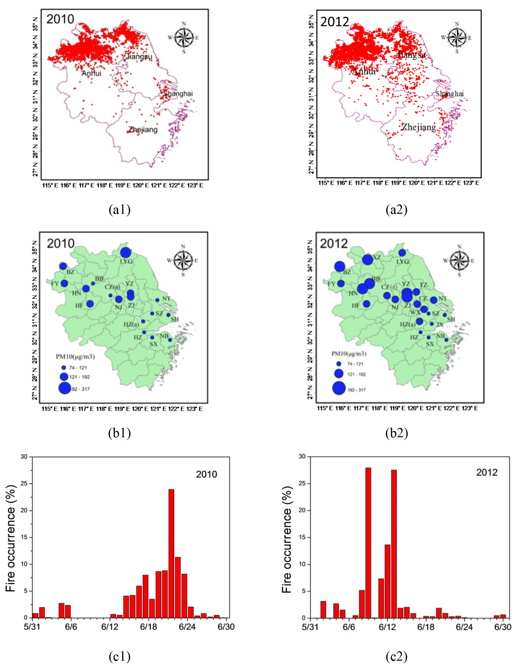
Figure 1(a) Spatial patterns of fire points in June 2010 and June 2012, (b) PM10 concentrations for the city level in the YRD in June 2010 and June 2012, and (c) temporal variations in daily fire occurrences in June 2010 and 2012. City abbreviations FY, BZ, BB, HN, HF, CZ(a), XZ, LYG, NJ, YZ, ZJ, TZ, NT, CZ, WX, SZ, HZ(a), JX, HZ, SX, NB and SH indicate Fuyang, Bozhou, Bengbu, Huainan, Hefei, Chuzhou, Xuzhou, Lianyungang, Nanjing, Yangzhou, Zhenjiang, Taizhou, Nantong, Changzhou, Wuxi, Suzhou, Huzhou, Jiaxing, Hangzhou, Shaoxing, Ningbo and Shanghai.
Figure 1 illustrated the spatial patterns of fire points (panels a1 and a2) in June 2010 and 2012, city-level PM10 concentrations in the YRD region in June 2010 and 2012 (panels b1 and b2), and temporal variations in daily fire occurrences in June 2010 and 2012 (panels c1 and c2). From 2005 to 2012, most OBB activities were found in June 2010 and 2012 and the northern YRD was the region with the intensive fire counts. Accordingly PM10 concentrations in northern YRD cities were higher than those in more developed and industrialized cities in the eastern YRD (e.g., Shanghai, Suzhou, Wuxi and Changzhou) because emissions of OBB overwhelmed those from other sources (Li et al., 2014; Huang et al., 2016). Therefore we constrained OBB emissions with observed PM10 concentrations in northern YRD cities including Xuzhou, Lianyungang, Fuyang, Bengbu, Huainan, Hefei, Chuzhou and Bozhou. Suggested by the monthly and daily distribution of fire counts (Figs. S3 and 1c), two strong OBB events were defined for 17–24 June 2010 and 8–14 June 2012, and other days in June 2010 and 2012 were defined as the non-OBB event period. For other years, OBB emissions were first scaled from the constrained emissions in 2010 and 2012 with the ratios of FRE for the corresponding year to that for 2010 and 2012, respectively, and then calculated as the average of the two. Remarkably, the correction of activity level was based on the comparisons of simulated and observed PM10 concentrations, and the emissions of other species were revised according to the changed activity level. The reliability of emission estimation for other species thus depended largely on the reliability of emission factors for PM10 and those species. Uncertainty would be introduced in the method and attributed to lack of sufficient and qualified domestic measurements on emission factors.
The traditional bottom-up method was used to calculate the initial emission input for all species (NMVOC emission factor was taken from the FRP-based method instead as those in the bottom-up method (Li et al., 2007) did not contain oxygenated VOCs). In contrast to application of a uniform percentage of CRBF within one province, however, percentage of CRBF for each city was calculated based on the fact that in the whole YRD and the fraction of FRP in the city to total YRD FRP to make the spatial distribution of OBB emissions consistent with that of FRP over the whole YRD region:
where i and k represent city and crop type, respectively; y indicates the year (2010 and 2012); and F, P, and FRP are the percentage of CRBF, crop production, and fire radiative power, respectively. The initial percentage of CRBF for total YRD (F(YRD,y) in Eq. 10) was expected to have a limited impact on the result and it was set at 10 %, smaller than those in previous studies (Streets et al., 2003; Cao et al., 2007; Wang and Zhang, 2008; Zhao et al., 2013; Xia et al., 2016; Zhou et al., 2017a).
2.4 Temporal and spatial distributions
The spatial and temporal patterns of OBB emissions in the three inventories were determined according to the FRP of agricultural fire points. The emissions of the mth grid in region u on the nth day in year y were calculated using Eq. (11):
where FRP(m,n) is the FRP of the mth grid on the nth day; FRP(u,y) and are the total FRP and OBB emissions of species j for region u in year y, respectively. The region u indicates city for the FRP-based and constraining methods, while it indicates province for the traditional bottom-up method since uniform percentages of CRBF were applied within the same province in the method.
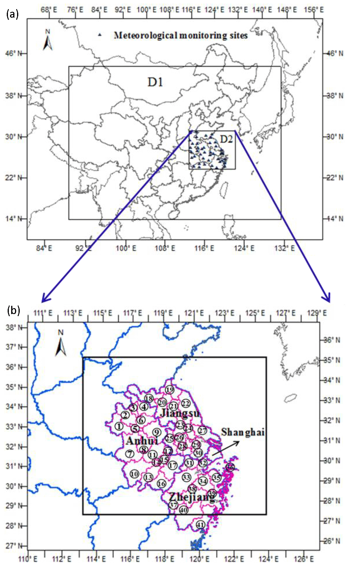
Figure 2Model domain and locations of 43 meteorological monitoring sites. The numbers of 1–41 represent the cities Fuyang, Bozhou, Huaibei, Suzhou, Huainan, Bengbu, Luan, Hefei, Chuzhou, Anqing, Chaohu, Maanshan, Chizhou, Tongling, Wuhu, Huangshan, Xuancheng, Xuzhou, Lianyungang, Suqian, Huai'an, Yancheng, Yangzhou, Taizhou, Nanjing, Zhenjiang, Nantong, Changzhou, Wuxi, Suzhou; Huzhou, Jiaxing, Hangzhou, Shaoxing, Ningbo, Zhoushan, Quzhou, Jinhua, Taizhou, Lishui and Wenzhou, respectively.
2.5 Configuration of air quality modeling
The Models-3 Community Multi-scale Air Quality (CMAQ) version 4.7.1 was applied to constrain OBB emissions and to evaluate OBB inventories with different methods. As shown in Fig. 2, one-way nested domain modeling was conducted, and the spatial resolutions of the two domains were set at 27 and 9 km, respectively, in Lambert conformal conic projection, centered at (110∘ E, 34∘ N) with two true latitudes 25 and 40∘ N. The mother domain (D1, 180×130 cells) covered most parts of China, Japan, and North and South Korea, while the second domain (D2, 118×97 cells) covered the whole YRD region. OBB inventories developed in this work were applied in D2. Emissions from other anthropogenic sources in D1 and D2 were obtained from the downscaled Multi-Resolution Emission Inventory for China (MEIC, http://www.meicmodel.org/, last access: 22 December 2018) with an original spatial resolution of . Population density was applied to relocate MEIC to each modeling domain. The biogenic emission inventory was from the Model Emissions of Gases and Aerosols from Nature developed under the Monitoring Atmospheric Composition and Climate project (MEGAN MACC; Sindelarova et al., 2014), and the emission inventories of Cl, HCl and lightning NOx were from the Global Emissions Initiative (GEIA; Price et al., 1997). Meteorological fields were provided by the Weather Research and Forecasting Model (WRF) version 3.4, and the carbon bond gas-phase mechanism (CB05) and AERO5 aerosol module were adopted. Other details on model configuration and parameters were given in Zhou et al. (2017b).
Meteorological parameters of the WRF model were compared with the observation dataset of the US National Climate Data Center (NCDC), as summarized in Table S6. For June 2010, the average biases between the two datasets were 0.06 m s−1 for wind speed, 9.84∘ for wind direction, 0.64 K for temperature and 2.99 % for relative humidity. The analogue numbers were 0.01 and 0.67 m s−1, 7 and 18.22∘, 0.91 and 0.43 K, and 3.1 and 0.07 %, respectively, for June 2012 and 2014, respectively. The meteorological parameters of this study were in compliance with the benchmarks derived from Emery et al. (2001) and Jiménez et al. (2006). Simulated daily PM10 concentrations were compared with observations for the non-OBB event period in June 2010 and 2012 in Table S7. The averages of NMBs and normalized mean errors (NMEs) were −19.2 % and 38.9 % for 17 YRD cities in June 2010 and 20.9 % and 33.9 % for 22 cities in June 2012, respectively. Simulated daily and hourly PM2.5, PM10 and CO concentrations were compared with the observation for the non-OBB event period in June 2014 in Tables S8 and S9. The hourly NMB of PM2.5 and PM10 was −29.9 % and −39.8 %, and the hourly NME of PM2.5 and PM10 was 49.8 % and 54.7 %. The model performance of PM2.5 and PM10 was similar to that derived by Zhang et al. (2006) in the US in general. The hourly NMB and NME of CO were −42.3 % and 48.3 %, and they were similar to those derived by Kota et al. (2018). As shown in Fig. S4, moreover, simulated hourly PM10 and PM2.5 concentrations were in good agreement with observations at four air quality monitoring sites in the YRD during the non-OBB event period in June 2012. The comparison thus implied the reliability of the emission inventory of anthropogenic origin used in this work, while underestimation might occur, indicated by the negative NMB.
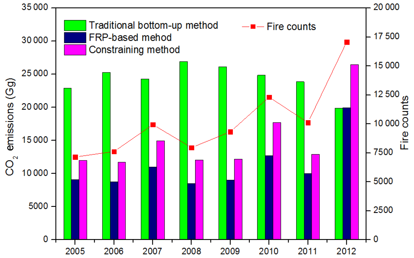
Figure 3Fire counts and CO2 emissions estimated with traditional bottom-up, FRP-based and constraining methods for YRD 2005–2012.
3.1 OBB emissions estimated with the three methods
OBB emissions estimated with the traditional bottom-up method for 2005–2012 were shown in Table S10. As emission factors were assumed unchanged during the period, similar interannual trends were found for all species and CO2 was selected as a representative species for further discussion. As shown in Fig. 3, CO2 emissions from the traditional bottom-up method were estimated to decrease from 23 000 in 2005 to 19 973 Gg in 2012, with a peak value of 27 061 Gg in 2008. In contrast, the number of fire points in YRD farmland increased from 7158 in 2005 to 17 074 in 2012. The fire counts detected from satellites thus did not support the effectiveness of OBB restriction by the government in the YRD before 2013. Table S11 presents the annual OBB emissions derived from the FRP-based method for 2005–2015 in the YRD region. Associated with fire counts, CO2 emissions were estimated to grow by 119.7 % from 2005 to 2012, with the largest and the second largest annual emissions calculated at 19 977 and 12 718 Gg for 2012 and 2010, respectively (Fig. 3). Similar temporal variability was found for fire counts, which increased by 138.5 % from 2005 to 2012, with the most and the second most counts found at 17 074 and 12 322 for 2012 and 2010, respectively.
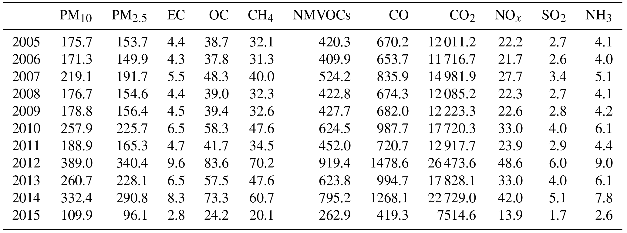
Table 1Constrained OBB emissions from 2005 to 2015 in the YRD (unit: Gg); OC: organic carbon; EC: elemental carbon.
With the constraining method, as shown in Fig. S5, the ratio of constrained mass of CRBF for 2012 to 2010 was 1.51, clearly lower than the ratios of original FRE (1.75) but close to the ratio of modified FRE for 2012 to 2010 (1.57). The comparison suggested that modified FRE better reflects the OBB activity in the YRD than the original FRE. In order to make the ratio of FRE for the two years be closer to the ratio of constrained mass of CRBF, an improved method was developed for calculating the FRE. Given the possible variation in FRPpeak hour between years, we obtained the diurnal cycle of total FRP of the YRD for 2005–2015 based on Gaussian fitting as shown in Fig. S6. The ratio of FRE for 2012 to 2010 was recalculated at 1.54, further closer to the ratio of constrained mass of CRBF. Therefore the ratios of FRE for another given year to 2012 and 2010 were calculated with this improved method and were then applied to emission scaling for that year. The constrained OBB emissions from 2005 to 2015 were summarized in Table 1. The interannual trend in constrained emissions was similar to those in fire counts and FRP-based emissions but different from that in emissions with the traditional bottom-up method, as shown in Fig. 3. It is usually difficult to collect accurate percentages of CRBF from the bottom-up method, as it demands intensive investigation in rural areas. In addition, the percentages of CRBF were not updated for each year, and the same percentages were commonly applied for years without sufficient data support from local surveys.
The constrained CO2 emissions for Jiangsu, Anhui, Zhejiang and Shanghai were calculated at 5790, 4699, 1104 and 419 Gg in 2005, accounting for 48.2 %, 39.1 %, 9.2 % and 3.5 % of total OBB emissions in the YRD, respectively. The analogue numbers for 2012 were 7345, 16 159, 2574 and 394 Gg and 27.7 %, 61.0 %, 9.7 % and 1.5 %, respectively. Jiangsu and Anhui were found to contribute the most to OBB emissions in the YRD for 2005 and 2012, respectively. In the traditional bottom-up method, however, Anhui was estimated to contribute the most for both years. City-level OBB emissions estimated with the three methods were summarized in Table S12–S14. With the constraining method, in particular, the largest CO2 emissions were found in Suzhou (1708 Gg) of Anhui and Lianyungang (1578 Gg) and Xuzhou (1401 Gg) of Jiangsu in 2005, accounting for 14.2 %, 13.1 % and 11.7 % of the total emissions, respectively. In 2012, Suzhou, Bozhou of Anhui and Xuzhou of Jiangsu were identified as the cities with the largest emissions, with the values estimated at 5007, 2433 and 2109 Gg, respectively. Depending on distribution of fire points, the shares of OBB emissions by city were close between the constraining and FRP-based methods, and large emissions concentrated in the north of the YRD. Based on surveyed percentages of CRBF and crop production, in contrast, the emission shares by city in the traditional bottom-up method were clearly different from the other two, and emissions were concentrated in Anhui cities with a high crop production level.
The average annual emissions of CO2 for 2005–2011 with the traditional bottom-up method were 87.0 % larger than those in the constraining method and the emissions for 2012 were 24.6 % smaller than those in the constraining method. Given the same sources of emission factors for all species except NMVOCs, the discrepancies of OBB emissions for most species between constraining and traditional bottom-up methods come from the activity levels (i.e., percentages of CRBF and crop production). The average annual constrained emissions from 2005 to 2015 were larger than those derived with the FRP-based method for all species except elemental carbon (EC), CH4 and NH3 since the average annual mass of CRBF from the constraining method was 36.9 % larger than those from the FRP-based method for these years, as shown in Fig. S7.
The percentage of CRBF is an important parameter to judge OBB activity and to estimate emissions. In addition to the investigated values applied in the traditional bottom-up approach, the percentages of CRBF were recalculated based on the constrained emissions at the provincial level and were shown in Fig. S8. The largest and smallest percentages of CRBF in the whole YRD region were estimated at 18.3 % in 2012 and 8.1 % in 2006, respectively. The interannual trend in percentages of CRBF for the YRD was closest to that for Anhui Province, as the province dominated the crop burning in the region. The different interannual trends by province were strongly influenced by agricultural practice and government management. Agricultural practice could be associated with income level and mechanization level. Increased income would lead to more crop residue discarded and burned in the field, while development of mechanization would lead to less. The constrained percentages of CRBF for Shanghai increased from 2005 to 2007 and declined after 2007, while those for Jiangsu decreased from 2005 to 2008 and increased after 2008. Increasing trends were found for the percentages of CRBF for Anhui and Zhejiang from 2005 to 2012, and they might result largely from growth of farmers' income. Note that percentages of CRBF for all provinces except Zhejiang decreased significantly in 2008, attributed largely to the measures of air quality improvement for the Beijing Olympic Games. Shanghai was the only one with its percentage of CRBF significantly reduced in 2010, resulting mainly from the air pollution control for Shanghai World Expo in that year. Compared to the percentages of CRBF used in the bottom-up method, the constrained ones of Anhui and Jiangsu for all the years except 2012 were smaller, leading to lower constrained OBB emissions than bottom-up ones in those years.
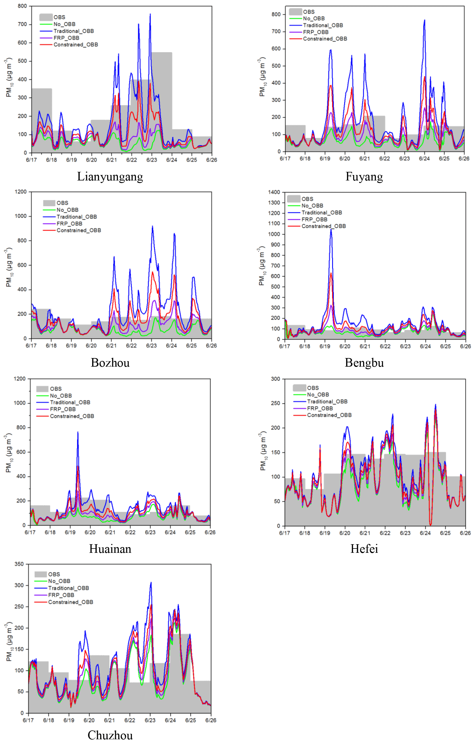
Figure 4Observed 24 h averaged PM10 concentrations and simulated hourly PM10 concentrations without OBB emissions (No_OBB) and with OBB emissions based on traditional bottom-up (Traditional_OBB), FRP-based (FRP_OBB) and constraining (Constrained_OBB) methods in Lianyungang, Fuyang, Bozhou, Bengbu, Huainan, Hefei and Chuzhou during 17–25 June 2010.
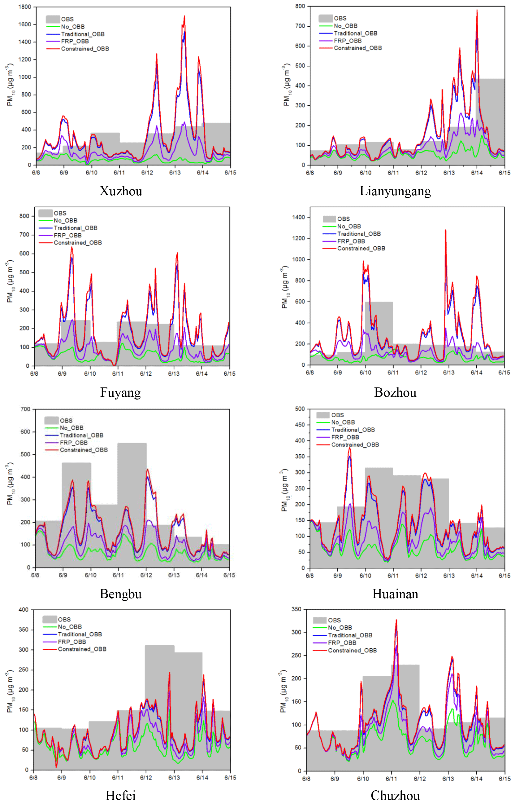
Figure 5Observed 24 h averaged PM10 concentrations and simulated hourly PM10 concentrations without OBB emissions (No_OBB) and with OBB emissions based on traditional bottom-up (Traditional_OBB), FRP-based (FRP_OBB) and constraining (Constrained_OBB) methods in Xuzhou, Lianyungang, Fuyang, Bozhou, Bengbu, Huainan, Hefei and Chuzhou during 8–14 June 2012.
The constrained percentages of CRBF and straw yields for 2012 were shown by city in Fig. S9, and clear inconsistency in spatial distributions can be found. The percentage of CRBF was not necessarily high for a city with large straw production. For instance, straw production of Yancheng was higher than most other cities, but its percentage of CRBF was 5.7 % and lower than most other cities. Through linear regression, the correlation coefficient was calculated at only 0.06 between the constrained percentage of CRBF and straw yield at the city level. The poor correlation between them thus suggested that large uncertainty could be derived if a uniform percentage of CRBF was applied to calculate OBB emissions for cities within a given province, as we did in the traditional bottom-up methodology.
3.2 Evaluation of the three OBB inventories with CMAQ
Figures 4 and 5 illustrate the observed 24 h averaged and simulated hourly PM10 concentrations for selected YRD cities in 17–25 June 2010 and 8–14 June 2012, respectively. Four emission cases, i.e., inventory without and with OBB emissions estimated using the three methods, were included. The simulated PM10 concentrations without OBB emissions were significantly lower than observation for all cities, implying that OBB was an important source of airborne particulates during the two periods. Simulations with OBB emissions derived from the three methods performed better than those without OBB emissions for most cities during 17–25 June 2010 and all cities during 8–14 June 2012. The best performance was found for simulations with constrained OBB emissions in most cities during the two periods, and the high PM10 concentrations were generally caught by CTM for the concerned OBB events. In 2010, the observed high concentrations were simulated with constrained emissions in Lianyungang during 21–23 June, and Fuyang and Huainan during 19–21 June. In 2012, the observed high concentrations were caught with constrained emissions in Xuzhou during 12–14 June, Lianyungang during 13–14 June, Fuyang during 11–12 June, Bozhou during 10 June and Chuzhou during 11–12 June. The results thus indicated that fire points could principally capture the temporal and spatial distribution of OBB emissions. Overestimation still existed with constrained OBB emissions for the cities with intensive fire points (e.g., Xuzhou, Bozhou, and Fuyang in 2012 and Bengbu in 2010), while underestimation commonly existed for cities with fewer fire points (e.g., Hefei, Chuzhou and Huainan in 2010 and 2012). Due to limitation of MODIS observation, fires at moderate to small scales could not be fully detected (Giglio et al., 2003; Schroeder et al., 2008); thus the spatial allocation of OBB emissions based on FRP could possibly result in more emissions than actually in areas with intensive fire points. Moreover, we used PM2.5, PM10 and CO concentrations (which were available since 2013) to evaluate the model performances when the constrained, FRP-based or no-OBB emissions were applied in CTM for an OBB event during 7–13 June 2014. Figures S10 and S11 illustrate the observed and simulated hourly concentrations for PM2.5 and PM10 in selected YRD cities, respectively. The best performance was found for simulations with the constrained OBB emissions in most cities during the period, and the peak particle concentrations were generally caught by CTM. The observed high concentrations were simulated with the constrained emissions in Lianyungang and Suqian on 12 June and Huai'an and Yancheng on 13 June. Figure S12 illustrates the observed and simulated hourly concentrations for CO in selected YRD cities, respectively. The best performance was found for simulations with the constrained OBB emissions in most cities during the period, and the observed high CO concentrations were simulated with the constrained emissions in Xuzhou and Huai'an on 13 June.
The NMB and NME between observed and simulated PM2.5 and PM10 concentrations are shown in Table 2. In most cases, the NMB and NME with constrained OBB emissions were smaller than those with other OBB emissions, implying the best guess of OBB emissions obtained through the constraining method combining CTM and ground observations. The simulated PM2.5 and PM10 concentrations using FRP-based OBB emissions were smaller than observations for the three periods, due mainly to the mass of CRBF being underestimated. The results thus indicated that OBB emissions might be underestimated with the FRP-based method in 2010, 2012 and 2014 since many small fires in the YRD were undetected in MODIS active fire detection products. The probability of MODIS detection was strongly dependent upon the temperature and area of the fire being observed. The average probability of detection for tropical savanna was 33.6 % when the temperature of fire was between 600 and 800 ∘C and the area of fire was between 100 and 1000 m2 (Giglio et al., 2003). In the YRD region, on the one hand, the fire temperature of crop residue burned in fields was relatively low. On the other hand, nearly 100 farmers were possibly located in a single 1×1 km MODIS pixel (Liu et al., 2015), and a farmer commonly owned croplands of several hundred square meters. Therefore many fire pixels in the YRD might not be detected, leading to underestimation in the total FRE. The simulated PM10 concentrations using traditional bottom-up OBB emissions were higher than observations in 2010 but lower in 2012. The results thus implied the growth in OBB emissions from 2010 to 2012 could not be captured by the traditional bottom-up method, attributed partly to application of an unreliable percentage of CRBF. We further selected the performance of CMAQ modeling in the US (Zhang et al., 2006) as the benchmark for PM2.5 and PM10 simulation. As can be seen in Table 2, the NMBs and NMEs for most cases with the constrained OBB emissions were close to those by Zhang et al. (2006). The NMEs for hourly PM2.5 and PM10 were slightly larger. Given the larger uncertainty in the emission inventory of anthropogenic sources for China and the uncertainty in spatial and temporal distribution of OBB emissions due to the satellite detection limit, we believe the model performance with the constrained OBB emissions was improved and acceptable. The NMB and NME between observed and simulated CO concentrations are shown in Table S15. Similar to PM2.5 and PM10, the NMBs and NMEs between observed and simulated CO concentrations with constrained OBB emissions were smaller than those with FRP-based OBB emissions or without OBB emissions, implying the advantage of constrained OBB emissions against other inventories.
Table 2Model performance statistics for concentrations of PM2.5 and PM10 from observation and CMAQ simulation without OBB emissions (No_OBB) and with OBB emissions based on traditional bottom-up (Traditional_OBB), FRP-based (FRP_OBB) and constraining methods (Constrained_OBB) for the three OBB events of June 2010, 2012 and 2014.
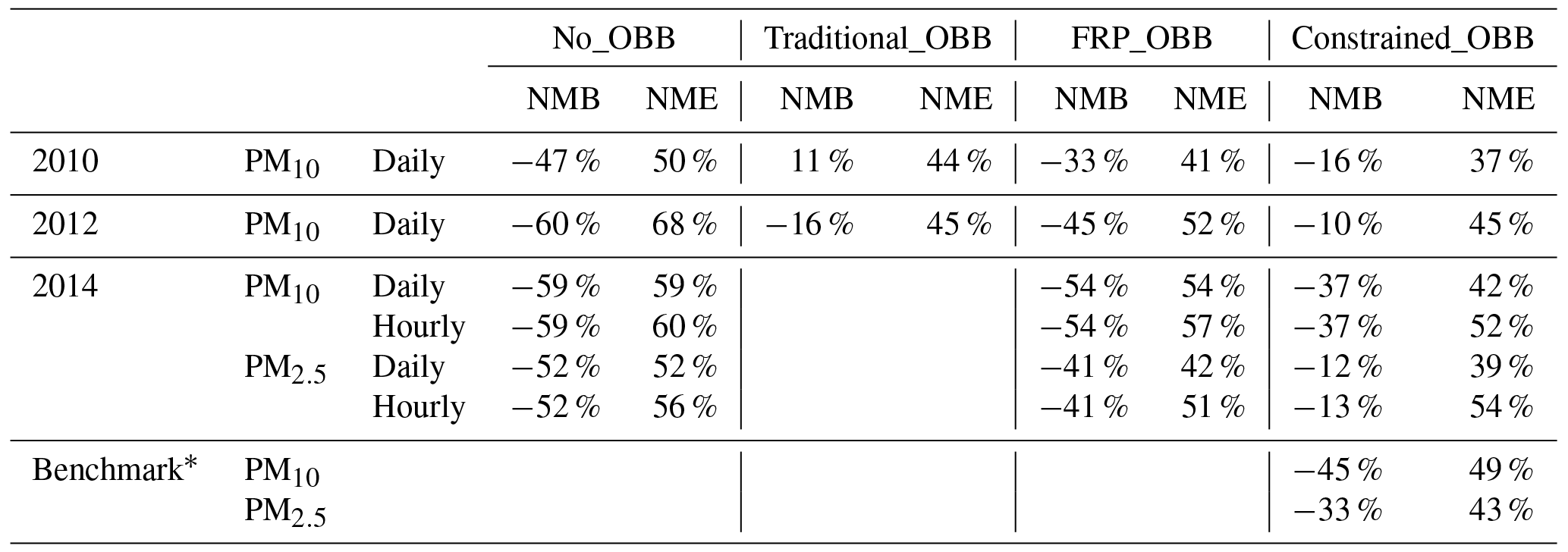
* From Zhang et al. (2006). NMB and NME were calculated using the following equations (P and O indicate the results from modeling prediction and observation, respectively): ; .
3.3 Comparisons of different methods and studies
We selected CO to compare emissions in this work and other inventories for the YRD, given the similar emission factors of CO applied in different studies. CO emissions from the three methods in this study were compared with GFASv1.0 (Kaiser et al., 2012), GFEDv3.0 (van der Werf et al., 2010), GFEDv4.1 (Randerson et al., 2018), Wang and Zhang (2008), Huang et al. (2012), Xia et al. (2016), and Zhou et al. (2017a), as shown in Fig. 6. The emissions from Wang and Zhang (2008), Huang et al. (2012), Xia et al. (2016), and Zhou et al. (2017a) were derived with the traditional bottom-up method, while GFASv1.0, GFEDv3.0 and GFEDv4.1 were based on FRP and BA methods. In particular, emissions from small fires were included in GFEDv4.1. Similar interannual variations were found for emissions derived from FRP measurement including the constrained and FRP-based emissions in this work, GFAS v1.0 and GFED v4.1, while those of GFEDv3.0 and Xia et al. (2016) were different. The percentages of CRBF were assumed unchanged during the study period in Xia et al. (2016); thus the temporal variation in OBB emissions was associated with the change in annual straw production.

Figure 6Annual CO emissions from OBB in the YRD obtained in this work and other studies from 2005 to 2012.
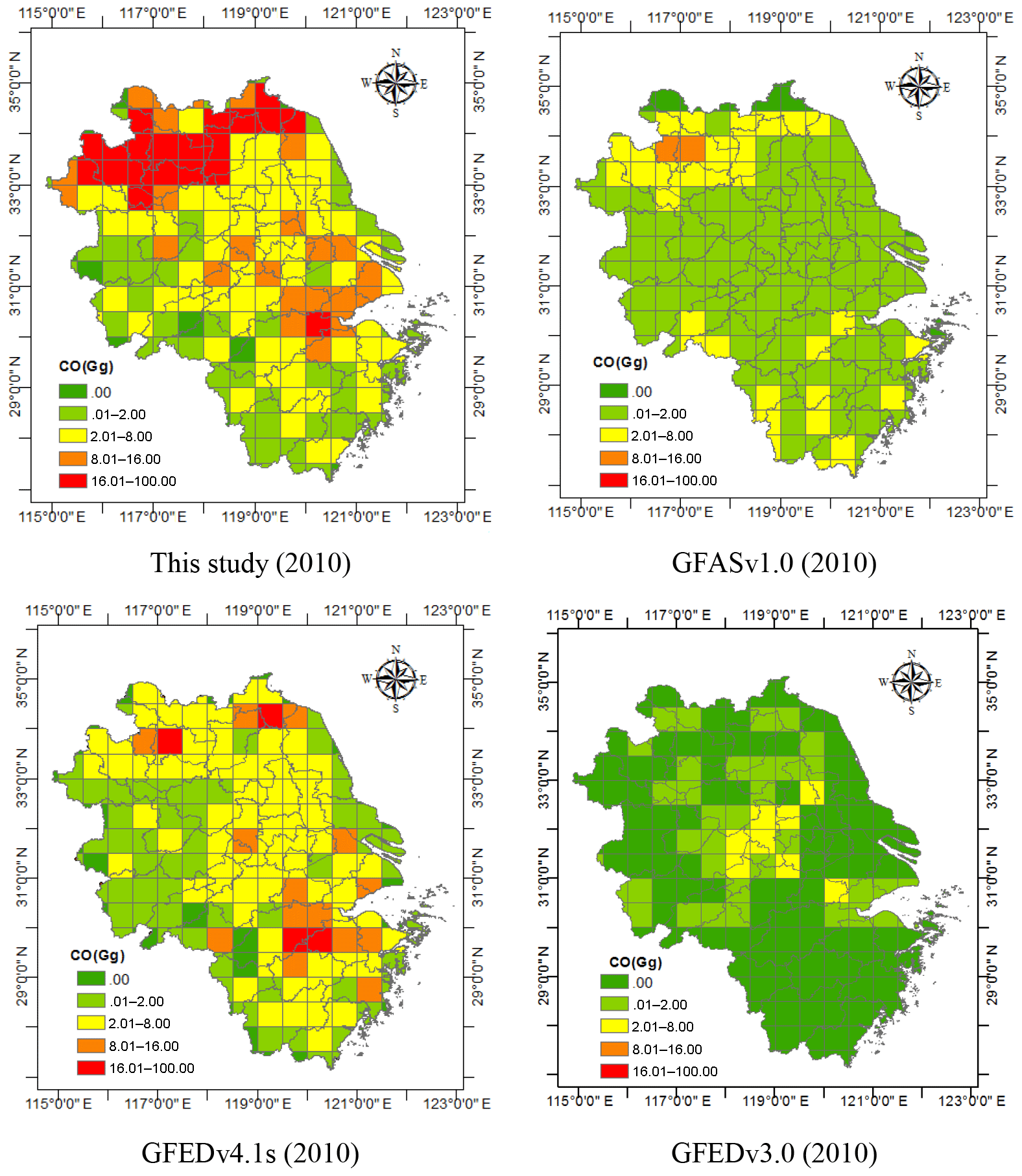
Figure 7Spatial distributions of CO emissions from OBB obtained in this work (constraining method), GFAS v1.0, GFED v3.0 and GFED v4.1s in 2010 (Horizontal resolution: ).
The constrained CO emissions in this work were lower than other studies using the traditional bottom-up method (Wang and Zhang, 2008; Huang et al., 2012; Xia et al., 2016) and higher than those based on burned area and FRP derived from satellites (GFEDv3.0, GFASv1.0, GFEDv4.1). In particular, the average annual constrained emissions from 2005 to 2012 were 3.9, 0.5 and 15.0 times larger than those in GFASv1.0, GFEDv4.1s and GFEDv3.0, respectively. The constrained emissions were closest to GFED v4.1s, which included small fires. Since the area of farmland belonging to individual farmers was usually small, small fires were expected to be important sources of OBB emissions in the YRD. GFEDv4.1s might still underestimate OBB emissions due to the omission errors for the small fires in MODIS active fire detection products (Schroeder et al., 2008). In addition, the constrained CO emission for 2013 was 31.5 % larger than those by Qiu et al. (2016) calculated based on burned area from satellite observations. The average annual CO emissions from 2005 to 2012 with the constraining method were 57.2 % smaller than Xia et al. (2016), and the constrained emissions for 2006 were respectively 27.6 % and 56.9 % lower than those by Huang et al. (2012) and Wang and Zhang (2008). It implied again that the emissions derived from traditional bottom-up method might be overestimated. Moreover, discrepancy in estimations for the same year between Huang et al. (2012) and Wang and Zhang (2008) with the traditional bottom-up method resulted mainly from application of different percentages of CRBF, implying that calculation of OBB emissions was sensitive to the parameter with the bottom-up approach.
The spatial distribution of constrained emissions in this work and those in GFASv1.0, GFEDv3.0 and GFEDv4.1s were illustrated in Fig. 7. Intensive OBB emissions in GFEDv3.0 were mainly found in parts of Anhui, Jiangsu and Shanghai, while the constrained emissions, GFEDv4.1s and GFASv1.0 emissions occurred in most YRD regions in accordance with the distribution of fire points. Therefore, GFEDv3.0 might miss a large number of burned areas, leading to underestimation in emissions and bias in spatial distribution.
In order to understand the discrepancies of emissions for different species in this work and other inventories, the emissions of 2010 derived from the three methods in this study, GFASv1.0, GFEDv3.0, GFEDv4.1s and Xia et al. (2016) were summarized in Table 3. Similar to CO, the constrained emissions for all species in this work were lower than Xia et al. (2016) and OBB emissions of this study based on the traditional bottom-up method. The constrained emissions for all species in this work were larger than GFASv1.0 and those for all species except NH3 were larger than GFEDv3.0 and GFEDv4.1s. In addition, the constrained emissions for most species were lower than the emissions from Huang et al. (2012), Wang and Zhang (2008), and Xia et al. (2016) using the traditional bottom-up method in 2006. In most cases, the discrepancy in activity levels among studies was larger than that in emission factors. Specifically, the OBB emissions for all species in the FRP-based (WSE) method were smaller than those derived with the bottom-up method. The differences in OBB emissions between the bottom-up and FRP-based (WSE) methods were larger than 50 % of those between the bottom-up and the original FRP-based method with different emission factors for most species. This indicated that the discrepancy in activity levels contributed the most to the difference in OBB emissions between the two methods.
Table 3OBB emissions in the YRD derived from this work and other studies in 2010 (unit: Gg).
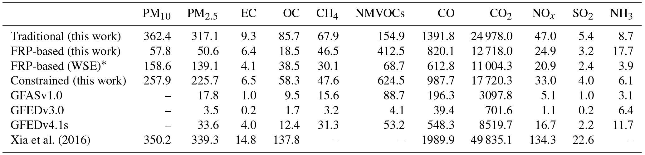
* FRP-based (WSE): the OBB emissions were estimated with the FRP-based method, applying the same emission factors used in the bottom-up method. The emission factors were obtained by weighting emission factors in the bottom-up method with the masses of various crop types.
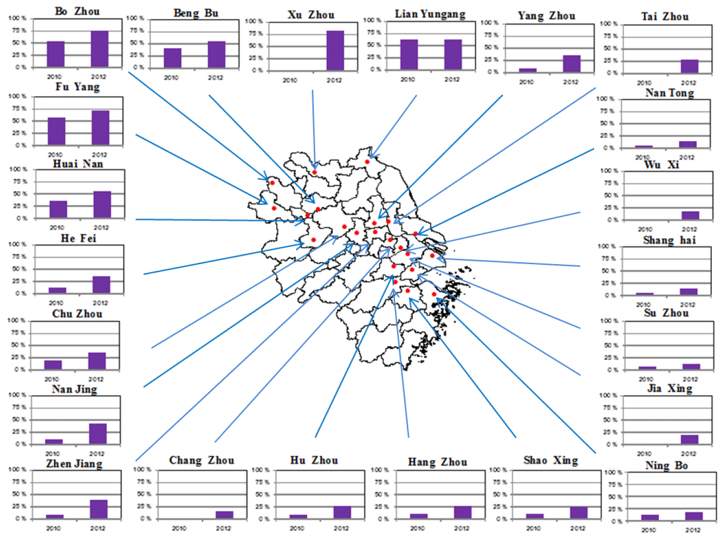
Figure 8The contribution of OBB to PM10 concentrations for different YRD cities during OBB events in June 2010 and 2012.
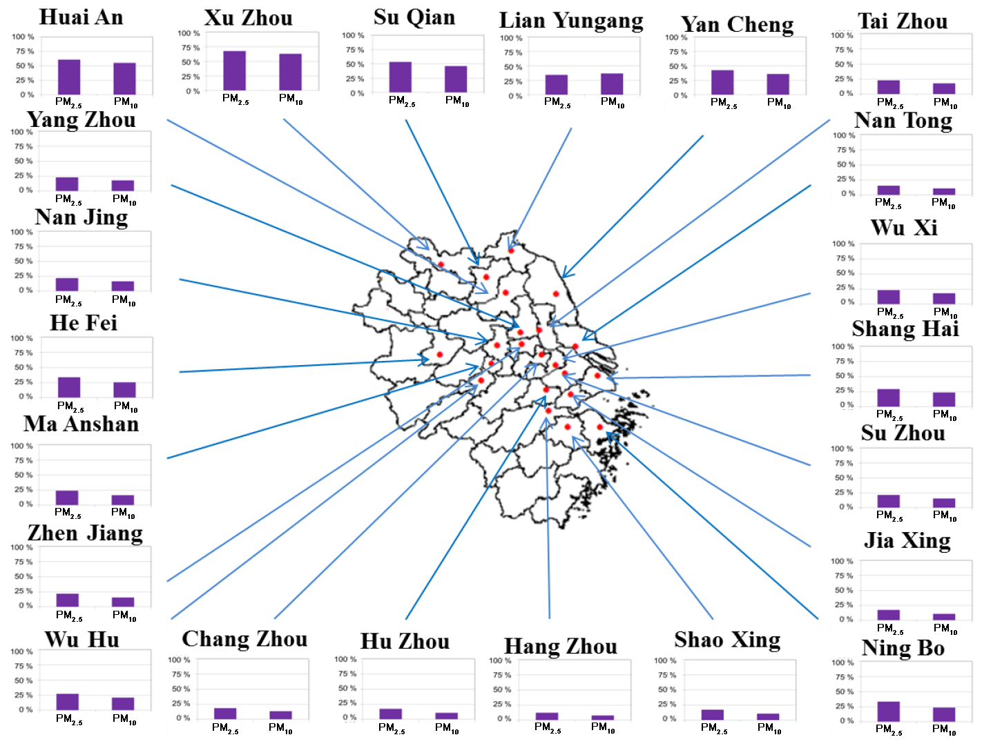
Figure 9The contribution of OBB to PM2.5 and PM10 concentrations for different YRD cities during the OBB event in June 2014.
Resulting from the different sources of emission factors, the discrepancies among studies or methods varied greatly by species. For PM10 and PM2.5, as an example, the emissions by Xia et al. (2016) were respectively 35.8 % and 50.3 % higher than constrained emissions in 2010. The discrepancies for SO2 and NOx were larger: the emissions by Xia et al. (2016) were 4.7 and 3.1 times larger than our constrained emissions, respectively. Moreover, the constrained NMVOC emission was 152.5 and 10.7 times larger than that of GFEDv3.0 and GFEDv4.1s in 2010, as the emission factors of GFEDv3.0 and GFEDv4.1s did not contain oxygenated VOCs. In contrast, the constrained NH3 emission was 4.7 % and 47.9 % smaller than that of GFEDv3.0 and GFEDv4.1s. The comparisons indicated that emission factors were important sources of uncertainties in estimation of OBB emissions with different methods.
3.4 Contribution of OBB to particulate pollution and its influencing factors
The BFM (Dunker et al., 1996) was used to analyze the contributions of OBB to PM10 pollution for the two OBB events, 17–24 June 2010 and 8–14 June 2012. Simulated PM10 concentrations with and without constrained OBB emissions were compared, and the difference indicated the contribution from OBB as shown by city in Fig. 8. The average contribution on 8–14 June 2012 was estimated at 37.6 % (56.7 µg m−3) for 22 cities in the YRD, and the contribution for 17–24 June 2010 was smaller at 21.8 % (24.0 µg m−3) for 17 cities. Our result for 2012 was nearly the same as that for five YRD cities in 2011 (37.0 %) by Cheng et al. (2014). Using the BFM, the contribution of OBB emissions to PM10 concentrations was estimated to increase by 136.3 % from 2010 to 2012 in this work, and the growth rate was larger than that of OBB emissions (50.8 %). Therefore, factors other than emissions (e.g., meteorology) could also play an important role in elevating the contribution of OBB to ambient particle pollution. For example, the average precipitation on 8–14 June 2012 was 36 % lower than that on 17–24 June 2010, exaggerating the particle pollution during the OBB event. For the OBB event during 7–13 June 2014, the contributions of OBB to both PM2.5 and PM10 concentrations were shown by city in Fig. 9. The average contributions of PM2.5 and PM10 were estimated at 29 % and 23 % for 22 cities in the YRD, indicating again that the OBB was an important source of ambient particles. OBB contribution to PM10 for 2014 was smaller than that for 2012, attributed mainly to the reduced straw burning in cropland.
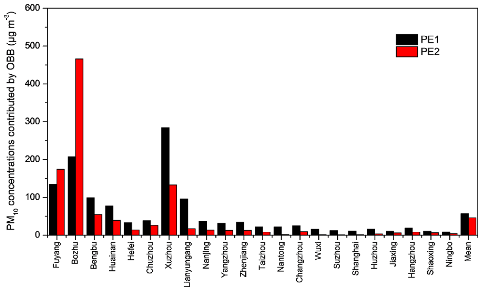
Figure 10PM10 concentrations contributed by OBB for different YRD cities on 8–14 June (PE1) and 22–28 June (PE2) 2012.
The average contributions of OBB for 2012 were estimated at 55.0 % (98.4 µg m−3), 36.4 % (58.0 µg m−3), 23.6 % (12.9 µg m−3) and 14.4 % (11.2 µg m−3) for six cities of Anhui, 10 cities of Jiangsu, five cities of Zhejiang and Shanghai, respectively. For individual cities, large contributions of OBB for 2012 were found in Xuzhou, Bozhou, Fuyang and Lianyungang located in the northern YRD, reaching 82.3 % (284.3 µg m−3), 75.2 % (207.5 µg m−3), 71.9 % (134.7 µg m−3) and 63.5 % (96.2 µg m−3), respectively. Similarly, large contributions for 2010 were found in Lianyungang, Fuyang and Bozhou reaching 63.3 % (69.8 µg m−3), 58.2 % (71.9 µg m−3) and 78.8 % (53.6 µg m−3), respectively. In general the spatial distribution of contributions to PM10 mass concentrations was similar to that of fire points, confirming the rationality of constraining OBB emissions with observed PM10 concentration in cities in northern Anhui and Jiangsu. For PM2.5, the large contributions of OBB were found in Xuzhou, Huai'an and Suqian during the event in 2014, reaching 67.5 % (111.7 µg m−3), 60.7 % (50.6 µg m−3) and 53.2 % (49.6 µg m−3), respectively.
To explore the influence of meteorology on air pollution caused by OBB, we simulated PM10 concentrations for 8–14 June (PE1) and 22–28 June 2012 (PE2) with varied meteorology conditions but fixed OBB emissions (i.e., constrained emissions for 8–14 June 2012). Poorer meteorology conditions during PE1 than PE2 were found. The average wind speed in PE1 was 2.4 m s−1, 17 % lower than that in PE2. The average wind direction in PE1 was 168.3∘, close to south with polluted air in land. In contrast, the average wind direction in PE2 was 118.3∘, close to east with clean air from the ocean. The average precipitation in PE2 was 6.8 mm, 28 % higher than that in PE1. As shown in Fig. 10, the average contribution of OBB to PM10 concentrations for 22 cities in the YRD region was estimated at 56.7 µg m−3 for PE1, 23 % larger than that for PE2, and the contributions in most cities were much larger for PE1 than those for PE2, except for Bozhou and Fuyang. The comparisons thus suggest that air pollution caused by OBB would exaggerate under poorer meteorology conditions. To reduce air pollution caused by OBB in harvest season in the YRD, therefore, more attention should be paid to the OBB restriction on those days with unfavorable meteorology conditions such as calm wind and rainless periods.
To further analyze the influence of diurnal variation in emissions on air pollution caused by OBB, we simulated PM10 concentrations of 17–24 June 2010 with various diurnal curves of OBB emissions (i.e., those for 2010 and 2012). Constrained emissions were applied in the simulation. As shown in Fig. 11, the contributions of OBB to PM10 concentrations based on the diurnal curve of 2012 were larger than those based on 2010 for almost all YRD cities, and the average contribution for the 17 cities was calculated at 28.6 µg m−3 based on the diurnal curve of 2012, 10 % larger than that based on 2010. The contribution in Bozhou changed most (1.37 times larger with the 2012 curve), while those in Shanghai, Huzhou and Shaoxing changed the least. The time of peak value for OBB emissions in 2012 was 2.5 h later than 2010, indicating that the fraction of OBB emissions at night for 2012 would be larger than that for 2010. As the diffusion condition for air pollutants at night was usually worse than that during daytime, more OBB emissions at night would elevate its contribution to particle pollution. In the actuality, the supervision of OBB prohibition was usually conducted by the government during daytime; thus some farmers burned more crop residue at night to avoid the punishment. To improve the air quality in harvest season in the YRD, more attention should be paid to the OBB restriction at night.
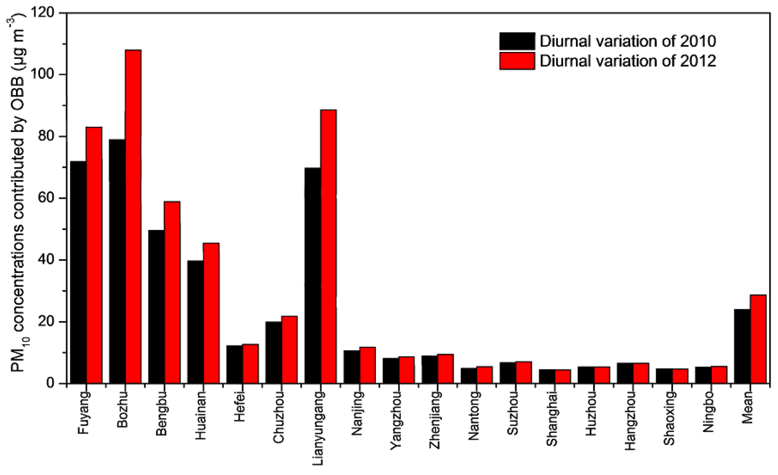
Figure 11PM10 concentrations contributed by OBB for different YRD cities based on the diurnal variations of 2010 and 2012 on 8–14 June 2010.
3.5 Uncertainty analysis
The uncertainties of OBB emissions estimated with bottom-up and FRP-based methods were quantified by species using a Monte Carlo simulation for 2012. A total of 20 000 simulations were performed and the uncertainties were expressed as 95 % confidence intervals (CIs) around the central estimates. The parameters contributing most to OBB emission uncertainty were also identified according to their contribution to the variance in Monte Carlo simulation.
For the traditional bottom-up method, parameters included crop productions, percentages of CRBF, straw-to-grain ratios, combustion efficiencies and emission factors. Crop production was directly taken from official statistical yearbooks (NBS, 2013) and its uncertainty was expected to be limited and not included in the analysis. As the percentage of CRBF was determined at half of the percentage of unused crop residue, its uncertainty was set at −100 % to +100 %. The combustion efficiencies were assumed within an uncertainty range of 10 % around the mean value according to de Zarate et al. (2005) and Zhang et al. (2008). Uncertainties of emission factors were obtained from original literatures from which they were derived. If the emission factor was derived from a single measurement, normal distribution was applied with the standard deviation directly taken from that work. If the emission factor was derived from multiple measurements and the samples were insufficient for data fitting, uniform distribution was tentatively applied with a conservative strategy to avoid possible underestimation of uncertainty: the uncertainty range of the given emission factor would be expanded according to Li et al. (2007) if the range originally from multiple studies was smaller than that in Li et al. (2007). Summarized in Table S16 was a database for emission factors and percentages of CRBF, with their uncertainties indicated by a probability distribution function (PDF). As shown in Table 4, the uncertainties of OBB emissions with the traditional bottom-up method for PM10, PM2.5, EC, organic carbon (OC), CH4, NMVOCs, CO, CO2, NOx, SO2 and NH3 in 2012 were estimated at −56 % to +70 %, −56 % to +70 %, −50 % to +54 %, −54 % to +73 %, −49 % to +58 %, −48 % to +59 %, −46 % to +73 %, −48 % to +60 %, −47 % to +87 %, −59 % to +138 % and −51 % to +67 %, respectively. For most species, the percentages of CRBF contributed the most to the uncertainties of OBB emissions, while emission factors were more significant to SO2 uncertainty.
Table 4The uncertainties of OBB emissions in the YRD indicated as 95 % CIs and the top two parameters contributing most to emission uncertainties based on traditional bottom-up and FRP-based methods for 2012. The percentages in the parentheses indicate the contributions of the parameters to the variances of emissions.
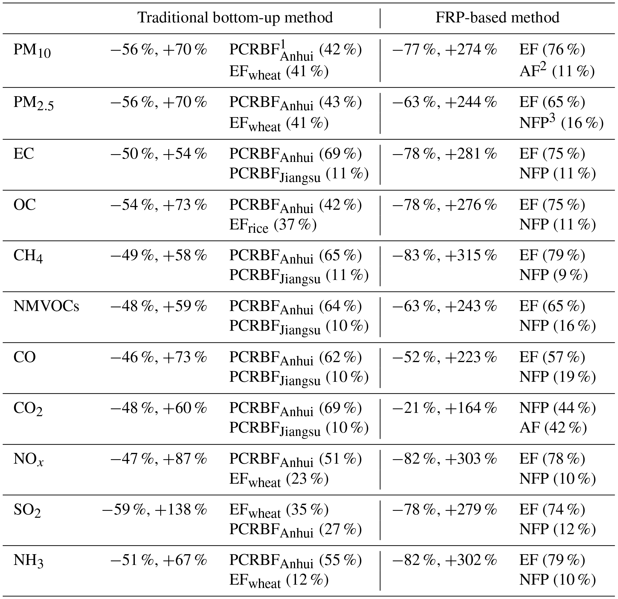
1 PCRBF, the percentage of crop residue burned in the field (the subscript indicates province). 2 AF, the average FRE of fire pixels. 3 NFP, the number of fire pixels. 4 MCRBF, the mass of crop residue burned in the field.
For the FRP-based method, parameters included total FRE, combustion conversion ratio and emission factors. Uncertainty of total FRE was associated with the FRP value, MODIS detection resolution and the methodology used to calculate FRE per fire pixel. Indicated by Freeborn et al. (2014), the coefficient of variation in MODIS FRP for a fire pixel was 50 %, but it declined to smaller than 5 % for the aggregation of over 50 MODIS active fire pixels. Given the large number of fire pixels for in the YRD (more than 17 000 in 2012), FRP was expected to contribute little to uncertainty of total FRE and could thus be ignored. Due to limitation of MODIS resolution and limited overpass times, many fires could not be detected and the number of fire pixels could be underestimated by 300 % for crop-dominant areas (Schroeder et al., 2008); therefore the uncertainty of the number of fire pixels was assumed to be 0 to +300 %. The method used to calculate FRE based on a single fire pixel assumed that fire lasted 1 day. Given the small cropland owned by one farmer in the YRD, individual fire normally lasted several hours, and FRE could be overestimated. As the total FRE in the FRP-based method was estimated to be 2.6 times larger than that from the constraining method based on the same number of fire pixels, we tentatively assumed the uncertainty range of FRE for 1 fire pixel to be 0 % to −72 %. The uncertainty of total FRE was then estimated at −17 % to +154 % (95 % CIs) based on the principle that total FRE was calculated as the number of fire pixels multiplied by average FRE. The uncertainty of the combustion conversion ratio was derived from Wooster et al. (2005) and Freeborn et al. (2008), while that of emission factors was taken from Akagi et al. (2011). As a result, uncertainties of the FRP-based inventory were estimated at −77 % to +274 %, −63 % to +244 %, −78 % to +281 %, −78 % to 276 %, −83 % to +315 %, −63 % to +243 %, −52 % to +223 %, −21 % to +164 %, −82 % to +303 %, −78 % to +279 % and −82 % to +302 % for PM10, PM2.5, EC, OC, CH4, NMVOCs, CO, CO2, NOx, SO2 and NH3 in 2012, respectively. Emission factors contributed most to the uncertainties of emissions for all species except CO2.
The uncertainty of constrained emissions could hardly be provided by Monte Carlo simulation, as the results were associated with CTM performance. In general, CTM performance could be influenced by emission estimates for sources other than OBB, chemistry mechanism of CTM, and temporal and spatial distribution of OBB emissions. The emission inventory of anthropogenic sources that incorporates the best available information of individual plants was expected to improve the CTM performance at the regional or local scale (Zhou et al., 2017b). The influence of the chemistry mechanism came mainly from secondary organic carbon (SOC) modeling. According to the Cheng et al. (2014) and Chen et al. (2017), the mass fraction of SOC to PM10 could reach 10 % during the OBB event in the YRD, and that part might not be well constrained with the approach we applied in this work. Similar to the FRP-based method, moreover, temporal and spatial distribution of OBB emissions based on FRP might not be entirely consistent with the reality, due to omission errors in the MODIS active fire detection products and limited times of satellite overpass as discussed earlier. Due to data limitation, finally, we relied on available PM10 concentrations in the current method. More data of multi-pollutant concentrations (e.g., PM2.5, OC and EC) with sufficient temporal and spatial resolution are greatly needed to better constrain the OBB emissions.
In general, uncertainties of OBB emissions with the traditional bottom-up method were estimated to be smaller than those with the FRP-based method, and uncertainties for CO2 and CO were usually smaller than other species in both methods attributed mainly to fewer variations in their emission factors. OBB emission estimation with the traditional bottom-up method could be improved if more accurate percentages of CRBF are obtained, and that with the FRP-based method could be improved when the omission error of satellites and the uncertainties of emission factors are reduced. Efforts should also be made to improve the CTM for better constraining the OBB emissions.
Taking the YRD in China as an example, we have thoroughly analyzed the discrepancies and their sources of OBB emissions estimated with traditional bottom-up, FRP-based and constraining methods. The simulated PM10 concentrations through CMAQ with constrained emissions were closest to available observation, implying the improvement of emission estimation with this method. The interannual variations in emissions with FRP-based and constraining methods were similar to the fire counts, while that with the traditional bottom-up method was not. This indicated that emissions with the traditional bottom-up method could not capture the real interannual trend in OBB emissions. The emissions of all species except NMVOCs based on the traditional bottom-up method might be overestimated in most years, attributed mainly to the elevated percentages of CRBF used in the method. The emissions with the FRP-based method might be underestimated in 2005–2015, attributed to the omission errors in the MODIS active fire detection products and thereby to the underestimation in mass of CRBF. The CO emissions with traditional bottom-up, FRP-based and constraining methods were compared with other studies. Similar temporal variations were found for the constrained emissions, emissions based on the FRP-based method, and emissions in GFASv1.0 and GFEDv4.1s. CO emissions based on the traditional bottom-up method in both this work and other studies were usually higher than those derived with the constraining method, and the CO emissions based on the FRP-based method in both this work and other studies were usually lower than those derived with the constraining method. It again demonstrated that the traditional bottom-up method might overestimate OBB emissions in the YRD and the FRP-based method might underestimate them. The contributions of OBB to particulate pollution in typical episodes were analyzed using the BFM in CMAQ modeling. The OBB emissions in 2012 were 51 % larger than those in 2010, while their contribution to average PM10 mass concentrations was estimated to increase by 136 % from 2010 to 2012. This indicated that the elevated contribution of OBB was not only attributed to growth in OBB emissions but was also influenced by the meteorology. Quantified with a Monte Carlo framework, the uncertainties of OBB emissions with the traditional bottom-up method were smaller than those with the FRP-based method. The uncertainties of emissions based on traditional bottom-up and FRP-based methods were mainly from the percentages of CRBF and emission factors, respectively. Further improvement on CTM for OBB events would help better constrain OBB emissions.
Limitations remained in this study. Given the difficulty in field investigation, annual CRBF used in the traditional bottom-up method was obtained from limited studies and it could not correctly reflect the real OBB activity. The reliability of OBB emissions with the FRP-based method depended largely on the detection resolution of the satellite. In the YRD where the burned areas of individual fires were small, many fires could not be detected by MODIS. The accuracy of constrained emissions depended largely on model performance and spatial and temporal distributions of OBB emissions derived from satellite-observed FRP. Therefore FRP-based and constraining methods may be improved if more reliable fire information is obtained. In addition, more measurements on local emission factors for OBB are suggested in the future to reduce the uncertainty of emissions.
The active fire data used in this study were obtained at https://earthdata.nasa.gov/active-fire-data (last access: 22 December 2018, Davies et al., 2009). The ground observed data used in this study were collected from http://106.37.208.233:20035/ (last access: 3 January 2019, CNEMC, 2013).
The supplement related to this article is available online at: https://doi.org/10.5194/acp-19-327-2019-supplement.
YY wrote the first draft and produced all the figures and tables. YZ provided useful comments and revised the paper.
The authors declare that they have no conflict of interest.
This work was sponsored the National Key Research and Development Program of
China (2016YFC0201507 and 2017YFC0210106), Natural Science Foundation of
China (91644220 and 41575142), Natural Science Foundation of Jiangsu
(BK20140020) and Special Research Program of Environmental Protection for
Common Wealth (201509004). The MCD14ML data were provided by LANCE FIRMS
operated by the NASA/GSFC/Earth Science Data and Information System (ESDIS)
with funding provided by NASA.
Edited by: Hailong Wang
Reviewed by: three
anonymous referees
Akagi, S. K., Yokelson, R. J., Wiedinmyer, C., Alvarado, M. J., Reid, J. S., Karl, T., Crounse, J. D., and Wennberg, P. O.: Emission factors for open and domestic biomass burning for use in atmospheric models, Atmos. Chem. Phys., 11, 4039–4072, https://doi.org/10.5194/acp-11-4039-2011, 2011.
Andreae, M. O. and Merlet, P.: Emission of trace gases and aerosols from biomass burning, Global Biogeochem. Cy., 15, 955–966, https://doi.org/10.1029/2000gb001382, 2001.
Bi, Y. Y.: Study on straw resources evaluation and utilization, Chinese Academy Agriculture Sciences, Beijing, China, 2010 (in Chinese).
Cao, G. L., Zhang, X. Y., Wang, D., and Zheng, F. C.: Inventory of atmospheric pollutants discharged from open biomass burning in China continent, Chinese Sci. Bull., 52, 1826–1831, 2007 (in Chinese).
Chen, D., Cui H. F., Zhao Y., Yin L., Lu, Y., and Wang, Q. G.: A two-year study of carbonaceous aerosols in ambient PM2.5 at a regional background site for western Yangtze River Delta, China, Atmos. Res., 183, 351–361, 2017.
Cheng, Z., Wang, S. X., Jiang, J. K., Fu, Q. Y., Chen, C. H., Xu, B. Y., Yu J. Q., Fu, X., and Hao J. M.: Long-term trend of haze pollution and impact of particulate matter in the Yangtze River Delta, China, Environ. Pollut., 182, 101–110, 2013.
Cheng, Z., Wang, S., Fu, X., Watson, J. G., Jiang, J., Fu, Q., Chen, C., Xu, B., Yu, J., Chow, J. C., and Hao, J.: Impact of biomass burning on haze pollution in the Yangtze River delta, China: a case study in summer 2011, Atmos. Chem. Phys., 14, 4573–4585, https://doi.org/10.5194/acp-14-4573-2014, 2014.
China National Environmental Monitoring Center (CNEMC): Chinese city air quality data, available at: http://106.37.208.233:20035/ (last access: 3 January 2019), 2013.
Crutzen, P. J. and Andreae, M. O.: Biomass burning in the tropics: Impact on atmospheric chemistry and biogeochemical cycles, Science, 250, 1669–1678, 1990.
Davies, D. K., Ilavajhala, S., Wong, M. M., and Justice, C. O.: Fire Information for Resource Management System: Archiving and Distributing MODIS Active Fire Data, IEEE Geosci. Remote Sens., 47, 72–79, 2009.
de Zarate, I. O., Ezcurra, A., Lacaux, J. P., Van Dinh, P., and de Argandona, J. D.: Pollution by cereal waste burning in Spain, Atmos. Environ., 73, 161–170, 2005.
Dunker, A. M., Morris, R. E., Pollack, A. K., Schleyer, C. H., and Yarwood, G.: Photochemical modeling of the impact of fuels and vehicles on urban ozone using auto oil program data, Environ. Sci. Technol., 30, 787–801, 1996.
Emery, C., Tai, E., and Yarwood, G.: Enhanced meteorological modeling and performance evaluation for two Texas episodes, Report to the Texas Natural Resources Conservation Commission, ENVIRON, International Corp, Novato, CA, 2001.
European Space Agency and Université Catholique de Louvain: GLOBCOVER 2009 Products Description and Validation Report, available at: http://due.esrin.esa.int/files/GLOBCOVER2009_Validation_Report_2.2.pdf (last access: 22 December 2018), 2011.
Fu, X., Wang, S. X., Zhao, B., Xing, J., Cheng, Z., Liu, H., and Hao, J. M.: Emission inventory of primary pollutants and chemical speciation in 2010 for the Yangtze River Delta region, China, Atmos. Environ., 70, 39–50, 2013.
Freeborn, P. H., Wooster, M. J., Roy, D. P., Cochrane, M. A.: Quantification of MODIS fire radiative power (FRP) measurement uncertainty for use in satellite based active fire characterization and biomass burning estimation, Geophys. Res. Lett., 41, 1988–1994, 2014.
Freeborn, P. H., Wooster, M. J., Hao, W. M., Ryan, C. A., Nordgren, B. L., Baker, S. P., and Ichoku, C.: Relationships between energy release, fuel mass loss, and trace gas and aerosol emissions during laboratory biomass fires, J. Geophys. Res., 113, D01301, https://doi.org/10.1029/2007jd008679, 2008.
Giglio, L., Descloitres, J., Justice, C. O., and Kaufman Y. J.: An enhanced contextual fire detection algorithm for MODIS, Remote Sens. Environ., 87, 273–282, 2003.
Giglio, L., Randerson, J. T., and van der Werf, G. R.: Analysis of daily, monthly, and annual burned area using the fourth generation global fire emissions database (GFED4), J. Geophys. Res.-Biogeo., 118, 317–328, https://doi.org/10.1002/jgrg.20042, 2013.
Guo, H., Cheng, T., Gu, X., Wang, Y., Chen, H., Bao, F., Shi, S. Y., Xu, B. R., Wang, W. N., Zuo, X., Zhang, X. C., and Meng, C.: Assessment of PM2.5 concentrations and exposure throughout china using ground observations, Sci. Total Environ., 1024, 601–602, 2017.
Hodzic A. and Duvel J. P.: Impact of biomass burning aerosols on the diurnal cycle of convective clouds and precipitation over a tropical island, J. Geophys. Res., 123, 1017–1036, https://doi.org/10.1002/2017JD027521, 2018.
Hooghiemstra, P. B., Krol, M. C., vanLeeuwen, T. T., van der Werf, G. R., Novelli, P. C., Deeter, M. N., Aben, I., and Röckmann, T.: Interannual variability of carbon monoxide emission estimates over South America from 2006 to 2010, J. Geophys. Res., 117, D15308, https://doi.org/10.1029/2012JD017758, 2012.
Huang, X., Ding, A., Liu, L., Liu, Q., Ding, K., Niu, X., Nie, W., Xu, Z., Chi, X., Wang, M., Sun, J., Guo, W., and Fu, C.: Effects of aerosol–radiation interaction on precipitation during biomass-burning season in East China, Atmos. Chem. Phys., 16, 10063–10082, https://doi.org/10.5194/acp-16-10063-2016, 2016.
Huang, X., Li, M., Li, J., and Song, Y.: A high-resolution emission inventory of crop burning in fields in China based on MODIS Thermal Anomalies/Fire products, Atmos. Environ., 50, 9–15, 2012.
Jiangsu Provincial Development and Reform Commission (JPDRC) and Jiangsu Provincial Agricultural Commission (JPAC): Comprehensive utilization planning of crop straw in Jiangsu, Nanjing, China, 2009 (in Chinese).
Jiménez, P., Jorba, O., Parra R., and Baldasano J. M.: Evaluation of MM5-EMICAT2000-CMAQ performance and sensitivity in complex terrain: High-resolution application to the northeastern Iberian Peninsula, Atmos. Environ., 40, 5056–5072, https://doi.org/10.1016/j.atmosenv.2005.12.060, 2006.
Kaiser, J. W., Heil, A., Andreae, M. O., Benedetti, A., Chubarova, N., Jones, L., Morcrette, J.-J., Razinger, M., Schultz, M. G., Suttie, M., and van der Werf, G. R.: Biomass burning emissions estimated with a global fire assimilation system based on observed fire radiative power, Biogeosciences, 9, 527–554, https://doi.org/10.5194/bg-9-527-2012, 2012.
Konovalov, I. B., Berezin, E. V., Ciais, P., Broquet, G., Beekmann, M., Hadji-Lazaro, J., Clerbaux, C., Andreae, M. O., Kaiser, J. W., and Schulze, E.-D.: Constraining CO2 emissions from open biomass burning by satellite observations of co-emitted species: a method and its application to wildfires in Siberia, Atmos. Chem. Phys., 14, 10383–10410, https://doi.org/10.5194/acp-14-10383-2014, 2014.
Kota S. H., Guo H., Myllyvirta L., Hu J. L., Sahu S. K., Garaga R., Ying Q., Gao A. F., Dahiya S., Wang Y., and Zhang H. L.: Year-long simulation of gaseousand particulate air pollutants in India, Atmos. Environ., 180, 244–255, https://doi.org/10.1016/j.atmosenv.2018.03.003, 2018.
Krol, M., Peters, W., Hooghiemstra, P., George, M., Clerbaux, C., Hurtmans, D., McInerney, D., Sedano, F., Bergamaschi, P., El Hajj, M., Kaiser, J. W., Fisher, D., Yershov, V., and Muller, J.-P.: How much CO was emitted by the 2010 fires around Moscow?, Atmos. Chem. Phys., 13, 4737–4747, https://doi.org/10.5194/acp-13-4737-2013, 2013.
Li, J. F., Song, Y., Mao, Y., Mao, Z. C., Wu, Y. S., Li, M. M., Huang, X., He, Q. C., and Hu, M.: Chemical characteristics and source apportionment of PM2.5 during the harvest season in eastern China's agricultural regions, Atmos. Environ., 92, 442–448, https://doi.org/10.1016/j.atmosenv.2014.04.058, 2014.
Li, X. H., Wang, S. X., Duan, L., Hao, J. M., Li, C., Chen, Y. S., and Yang, L.: Particulate and trace gas emissions from open burning of wheat straw and corn stover in China, Environ. Sci. Technol., 41, 6052–6058, 2007.
Liu, M. X., Song, Y., Yao H., Kang, Y. N., Li, M. M., Huang, X., and Hu, M.: Estimating emissions from agricultural fires in the North China Plain based on MODIS fire radiative power, Atmos. Environ., 112, 326–334, 2015.
National Bureau of Statistics (NBS): China Statistical Yearbook 2006–2013, China Statistics Press, Beijing, 2013 (in Chinese).
National Development and Reform Commission Office (NDRC), and National Environmental Protection Department (NEPD): Comprehensive utilization and burning of crop straw in China, Beijing, China, 2014 (in Chinese).
Price, C., Penner, J., and Prather, M.: NOx from lightning, Part I: Global distribution based on lightning physics, J. Geophys. Res.-Atmos., 102, 5929–5941, https://doi.org/10.1029/96JD03504, 1997.
Qiu, X. H., Duan, L., Chai, F. H., Wang, S. X., Yu, Q., and Wang, S. L.: Deriving high-resolution emission inventory of open biomass burning in China based on satellite observations, Environ. Sci. Technol., 50, 11779–11786, https://doi.org/10.1021/acs.est.6b02705, 2016.
Ran, L., Zhao, C., Geng, F., Tie, X., Peng, L., Zhou, G., Yu, Q., Xu, J., and Guenther, A.: Ozone photochemical production in urban Shanghai, China: Analysis based on groud level observations, J. Geophys. Res., 114, D15301, https://doi.org/10.1029/2008JD010752, 2009.
Randerson, J. T., van der Werf, G. R., Giglio, L., Collatz, G. J., and Kasibhatla, P. S.: Global Fire Emissions Database, Version 4.1, (GFEDv4), ORNL DAAC, Oak Ridge, Tennessee, USA, https://doi.org/10.3334/ORNLDAAC/1293, 2018.
Richter, A., Burrows, J. P., Nuss, H., Granier, C., and Niemeier, U.: Increase in tropospheric nitrogen dioxide over China observed from space, Nature, 437, 129–132, 2005.
Schroeder, W., Prins, E., Giglio, L., Csiszar, I., Schmidt, C., Morisette, J., and Morton, D.: Validation of GOES and MODIS active fire detection products using ASTER and ETM+ data, Remote Sens. Environ, 112, 2711–2726, https://doi.org/10.1016/j.rse.2008.01.005, 2008.
Shi, Y. S. and Yamaguchi, Y.: A high-resolution and multi-year emissions inventory for biomass burning in Southeast Asia during 2001–2010, Atmos. Environ., 98, 8–16, 2014.
Sindelarova, K., Granier, C., Bouarar, I., Guenther, A., Tilmes, S., Stavrakou, T., Müller, J.-F., Kuhn, U., Stefani, P., and Knorr, W.: Global data set of biogenic VOC emissions calculated by the MEGAN model over the last 30 years, Atmos. Chem. Phys., 14, 9317–9341, https://doi.org/10.5194/acp-14-9317-2014, 2014.
Streets, D. G. and Yarber, K. F.: Biomass burning in Asia: Annual and seasonal estimates and atmospheric emissions, Global Biogeochem. Cy., 17, 1099, https://doi.org/10.1029/2003GB002040, 2003.
Su, J. F., Zhu B., Kang, H. Q., Wang, H. N., and Wang T. J.: Applications of pollutants released form crop residues at open burning in Yangtze River Delta, Environ. Sci., 5, 1418–1424, 2012 (in Chinese).
van der Werf, G. R., Randerson, J. T., Giglio, L., Collatz, G. J., Mu, M., Kasibhatla, P. S., Morton, D. C., DeFries, R. S., Jin, Y., and van Leeuwen, T. T.: Global fire emissions and the contribution of deforestation, savanna, forest, agricultural, and peat fires (1997–2009), Atmos. Chem. Phys., 10, 11707–11735, https://doi.org/10.5194/acp-10-11707-2010, 2010.
Van Donkelaar, A., Martin, R. V., Brauer, M., Kahn, R., Levy, R., Verduzco, C., and Villeneuve, P. J.: Global estimates of ambient fine particulate matter concentrations from satellite-based aerosol optical depth: development and application, Environ. Health. Persp., 118, 847–855, 2010.
Vermote, E., Ellicott, E., Dubovik, O., Lapyonok, T., Chin, M., Giglio, L., and Roberts, G. J.: An method to estimate global biomass burning emissions of organic and black carbon from MODIS fire radiative power, J. Geophys. Res., 114, D18205, https://doi.org/10.1029/2008jd011188, 2009.
Wang, S. X. and Zhang, C. Y.: Spatial and temporal distributions of air pollutant emissions from open burning of crop residues in China, Sciencepaper Online, 5, 329–333, 2008 (in Chinese).
Wang, Y. C., Chen, F., Zhu, W., and Zen, Y. W.: Estimation and regional distribution of straw resources in Jiangsu province, Jiangsu Agricultural Sciences, 41, 305–310, 2013 (in Chinese).
Wiedinmyer, C., Akagi, S. K., Yokelson, R. J., Emmons, L. K., Al-Saadi, J. A., Orlando, J. J., and Soja, A. J.: The Fire INventory from NCAR (FINN): a high resolution global model to estimate the emissions from open burning, Geosci. Model Dev., 4, 625–641, https://doi.org/10.5194/gmd-4-625-2011, 2011.
Wooster, M. J., Roberts, G., Perry, G. L. W., and Kaufman, Y. J.: Retrieval of biomass combustion rates and totals from fire radiative power observations: FRP derivation and calibration relationships between biomass consumption and fire radiative energy release, J. Geophys. Res., 110, D24311, https://doi.org/10.1029/2005jd006318, 2005.
Xia, Y. M., Zhao, Y., and Nielsen, C. P.: Benefits of China's efforts in gaseous pollutant control indicated by the traditional bottom-up emissions and satellite observations 2000–2014, Atmos. Environ., 136, 43–53, 2016.
Xiao, Z. M., Zhang, Y. F., Hong, S. M., Bi, X. H., Jiao, L., Feng, Y. C., and Wang, Y. Q.: Estimation of the main factors influencing haze, based on a long-term monitoring Campaign in Hangzhou, China, Aerosol Air Qual. Res., 11, 873–882, 2011.
Xing, J., Mathur, R., Pleim, J., Hogrefe, C., Gan, C.-M., Wong, D. C., Wei, C., Gilliam, R., and Pouliot, G.: Observations and modeling of air quality trends over 1990–2010 across the Northern Hemisphere: China, the United States and Europe, Atmos. Chem. Phys., 15, 2723–2747, https://doi.org/10.5194/acp-15-2723-2015, 2015.
Zhang, H. F., Ye, X. G., Cheng, T. T., Chen, J. M., Yang, X., Wang, L., and Zhang, R. Y.: A laboratory study of agricultural crop residue combustion in China: Emission factors and emission inventory, Atmos. Environ., 42, 8432–8441, 2008.
Zhang, Y., Liu, P., Pun, B., and Seigneur, C.: A comprehensive performance evaluation of MM5-CMAQ for the Summer 1999 Southern Oxidants Study episode – Part I: Evaluation protocols, databases, and meteorological predictions, Atmos. Environ., 40, 4825–4838, 2006.
Zhao, Y., Zhang, J., and Nielsen, C. P.: The effects of recent control policies on trends in emissions of anthropogenic atmospheric pollutants and CO2 in China, Atmos. Chem. Phys., 13, 487–508, https://doi.org/10.5194/acp-13-487-2013, 2013.
Zheng, Y., Xue, T., Zhang, Q., Geng, G., Tong, D., Li, X., and He, K. B.: Air quality improvements and health benefits from China's clean air action since 2013, Environ. Res. Lett., 12, 114020, https://doi.org/10.1088/1748-9326/aa8a32, 2017.
Zhou, Y., Xing, X., Lang, J., Chen, D., Cheng, S., Wei, L., Wei, X., and Liu, C.: A comprehensive biomass burning emission inventory with high spatial and temporal resolution in China, Atmos. Chem. Phys., 17, 2839–2864, https://doi.org/10.5194/acp-17-2839-2017, 2017a.
Zhou, Y., Zhao, Y., Mao, P., Zhang, Q., Zhang, J., Qiu, L., and Yang, Y.: Development of a high-resolution emission inventory and its evaluation and application through air quality modeling for Jiangsu Province, China, Atmos. Chem. Phys., 17, 211–233, https://doi.org/10.5194/acp-17-211-2017, 2017b.