the Creative Commons Attribution 4.0 License.
the Creative Commons Attribution 4.0 License.
 | 12 Mar 2019
Long-term lidar observations of the gravity wave activity near the mesopause at Arecibo
Jonathan S. Friedman
Qihou Zhou
Xiongbin Wu
Jens Lautenbach
Using 11-year-long K Doppler lidar observations of temperature profiles in the mesosphere and lower thermosphere (MLT) between 85 and 100 km, conducted at the Arecibo Observatory, Puerto Rico (18.35∘ N, 66.75∘ W), seasonal variations of mean temperature, the squared Brunt–Väisälä frequency, N2, and the gravity wave potential energy (GWPE) are estimated in a composite year. The following unique features are obtained. (1) The mean temperature structure shows similar characteristics to an earlier report based on a smaller dataset. (2) Temperature inversion layers (TILs) occur at 94–96 km in spring, at ∼92 km in summer, and at ∼91 km in early autumn. (3) The first complete range-resolved climatology of GWPE derived from temperature data in the tropical MLT exhibits an altitude-dependent combination of annual oscillation (AO) and semiannual oscillation (SAO). The maximum occurs in spring and the minimum in summer, and a second maximum is in autumn and a second minimum in winter. (4) The GWPE per unit volume reduces below ∼97 km altitude in all seasons. The reduction of GWPE is significant at and below the TILs but becomes faint above; this provides strong support for the mechanism that the formation of upper mesospheric TILs is mainly due to the reduction of GWPE. The climatology of GWPE shows an indeed pronounced altitudinal and temporal correlation with the wind field in the tropical mesopause region published in the literature. This suggests the GW activity in the tropical mesopause region should be manifested mainly by the filtering effect of the critical level of the local background wind and the energy conversion due to local dynamical instability.


Gravity waves (GWs) are believed to be the primary force driving the large-scale circulation and coupling of different atmospheric layers due to their momentum and energy deposition when breaking or dissipating (Fritts and Alexander, 2003; Lindzen, 1981; Smith, 2012). GWs often originate from copious tropospheric sources and propagate upward. Their amplitudes grow rapidly with altitude under the condition of decreasing atmospheric density. GWs begin to break or dissipate in the mesosphere and lower thermosphere (MLT), where their influences have been shown to be strong by various observations (e.g., Baumgarten et al., 2015, 2017, 2018; Cai et al., 2014; Gardner and Liu, 2010; Li et al., 2010; Lu et al., 2009; Yuan et al., 2016). GWs are therefore an essential component in current general circulation models (GCMs) (e.g., Liu and Meriwether, 2004; Picone et al., 2002). Associated modeling studies have shown that including the effects of GWs is a key point in the simulation of realistic quasi-biennial and semiannual oscillations and other phenomena in the stratosphere and mesosphere (e.g., Dunkerton, 1982; Huang et al. 2010; Xu et al., 2006).
The upward propagation of GWs is often influenced by the background wind fields (e.g., Yiğit and Medvedev, 2015). The altitude ranges, in which GWs interact with the background winds to dissipate and deposit energy and momentum to the background, are of high interest to researchers. This mainly happens in the middle atmosphere near or between the stratopause and mesopause. Above 35 km altitude, the semiannual oscillation (SAO) shows a predominance in the annual variability of the zonal winds (e.g., Garcia et al., 1997; Hirota, 1980). The SAO phase of zonal winds shifts approximately 180∘ with the altitude increasing from the stratosphere to the mesosphere. The stratospheric SAO leads to a seasonal variation of filtering of the upward propagating waves, which results in a specific seasonal variation of GW activity in the mesosphere.
The mean zonal winds in the MLT have been measured by both ground-based radars (e.g., Garcia et al., 1997; Lieberman et al., 1993) and satellite-based instruments such as the High-Resolution Doppler Imager (HRDI), Wind Imaging Interferometer (WINDII), and the Microwave Limb Sounder (MLS) on board the Upper Atmosphere Research Satellite (UARS) or the Doppler Interferometer (TIDI) on board the Thermosphere Ionosphere Mesosphere Energetics and Dynamics (TIMED) satellite (e.g., Smith, 2012). They show different features of the zonal winds in the mesopause range from the tropical region to midlatitude regions. Garcia et al. (1997) and Smith (2012) showed that, for example, the westerly winds prevailed in the range 80–95 km both in January and July in the HRDI equatorial zonal wind, but it reversed below or above this range in the Northern Hemisphere. The monthly mean HRDI equatorial zonal wind showed that easterly winds were prevailing in equinox seasons in the 80–100 km altitude range, with the minimal wind speed occurring near 92 km, while the westerly winds prevailed in solstice seasons in the 80–94 km altitude range, with the maximal wind speed occurring near 88 km. The easterly winds prevail above 95 km in solstice seasons (Smith, 2012). Therefore, the zonal winds are low or zero around 92 km altitude in the tropical region. The zero-wind lines will enhance reduction or dissipation of zonal propagating gravity waves with low to moderate phase speed. There are also reports about the tropical MLT mean winds measured by ground-based radars (e.g., Guharay and Franke, 2011; Li, et al., 2012).
Temperature is a crucial parameter indicating the state of the atmosphere. To measure the temperature in the MLT region, satellite and lidar techniques have been developed in recent decades. Satellite measurements have the advantage of resolving large spatial-scale wave structures, but the short-term variability in dynamical features gets lost, while for the lidar measurements, they provide vertical profiles of temperature with a suitable temporal and vertical resolution at a particular location. Lidar data can resolve gravity waves with short and medium periods and their temporal development well. The perturbation or standard deviation from zonal mean temperature is often used as a wave activity indicator in the atmosphere. For instance, Offermann et al. (2006) use the temperature measured from CRISTA (CRyogenic Infrared Spectrometers and Telescopes for the Atmosphere) and from SABER (Sounding of the Atmosphere using Broadband Emission Radiometry) to investigate the global wave activity from the upper stratosphere to lower thermosphere. They showed quite different wave behaviors below and above their defined “wave turbopause” close to but lower than the mesopause. Below the turbopause, the propagation of the wave is significantly dissipated, while above that, the propagation of the wave is almost free.
The reduction of GW activity has also been presented by lidar temperature measurements at midlatitude sites (Mzé et al., 2014; Rauthe et al., 2008). Both Mzé et al. (2014) and Rauthe et al. (2008) showed that the GW activities presented an annual variation, with a maximum in winter and a minimum in summer; they reduced significantly at the upper mesosphere altitudes above ∼70 km in all seasons, while the reduction below ∼70 km is not so evident. Mzé et al. (2014) observed a nearly undamped propagation of GWs in summer in the low mesosphere. Meanwhile, Rauthe et al. (2008) also reported the weakest reduction occurring in the summer seasons. Since the effects of GWs in the numerical climate and weather prediction models are usually represented simply by parameterization (Kim et al., 2003), there are still large discrepancies between the model and measurement results (Geller et al., 2013). Therefore, more attention should be paid to the GW parameterization concerning these kinds of observations in the upper mesosphere and mesopause region to improve the model results.
Seasonal variations of GW activities based on lidar temperature measurements have been investigated at a few low-latitude sites (Chane-Ming et al., 2000; Li et al., 2010; Sivakumar et al., 2006). These studies used Rayleigh lidar data and focused mainly on the upper stratosphere and lower mesosphere in an altitude region from 30 to 80 km. They showed the SAO dominated the seasonal variability of GW activities, with maxima in both winter and summer and minima near the equinox. Li et al. (2010) related this to the dominant SAO in the mean zonal wind in the tropical stratosphere and lower mesosphere. Considering the different transition of the mean zonal wind in the range 80–95 km in the tropical region noted above, the seasonal variability of GW activity in the tropical upper mesosphere is expected to be different from either the lower altitudes or the midlatitude and high-latitude regions.
To the best of our knowledge, the seasonal variability of GW activity retrieved from mesospheric lidar temperature data with high temporal and vertical resolution has never been reported from a tropical location.
Such measurements of atmospheric temperature have been conducted with the K Doppler lidar located at the Arecibo Observatory (18.35∘ N, 66.75∘ W), Puerto Rico (Friedman and Chu, 2007; Yue et al., 2013, 2016). Since December 2003, the Arecibo Observatory K Doppler lidar has operated routinely, producing high-quality temperature data. In this report, we estimate the mean temperature, the squared Brunt–Väisälä frequency, N2, and the gravity wave potential energy (GWPE) and their annual variability from the temperature dataset. We find an altitude-to-altitude close relationship between the annual variability of the potential energy in this report and that of the mean zonal winds in the literature. Their implications for the GW activity in the MLT are discussed.
The Arecibo K Doppler lidar probes the potassium D1 line to deduce the potassium density and neutral air temperature simultaneously by employing the three-frequency technique (e.g., Friedman and Chu, 2007; Friedman et al., 2003). The temperature was obtained at 0.45∕0.9 km vertical and 10∕30 min temporal resolution, respectively (Friedman and Chu, 2007), and we unify them into profiles with resolutions of 0.9 km and 30 min in vertical and temporal dimensions, respectively. This data processing excludes the perturbations relevant to GWs with vertical wavelengths and observed periods less than 1.8 km and 1 h, respectively. Their exclusion may bias the deduced GW-associated potential energy estimations towards mid- and low-frequency GWs. The root mean square (rms) temperature errors are about 2 to 3 K at the peak of the K density layer and increase to about 10 K around 85 and 100 km (Friedman and Chu, 2007; Yue et al., 2017).
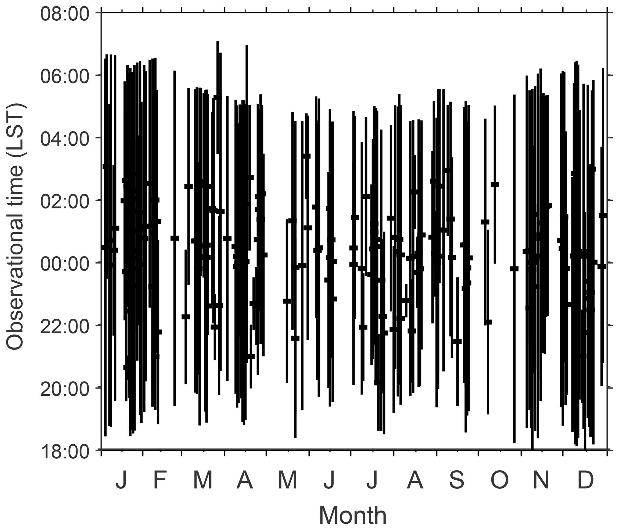
Figure 1Local time coverage of the temperature data observed by the K-Doppler lidar at Arecibo from December 2003 to January 2010, and from November 2015 to April 2017.
Measurements were only made at night in two periods, one from December 2003 to January 2010 and the other from November 2015 to April 2017. Data were available for every calendar month. Across the 11 years of the data collection period, 200 observing nights with a total of 1470 h of data were available at the time of preparing this report. The number of observation nights and hours varies from 4 nights and 28 h in October to 32 nights and 259 h in January. On average there are 16.7 nights and 122.5 h of observations each month. The statistics for the temperature observations used are plotted in Fig. 1 and the numbers of observational nights and durations are summarized for each month in Table 1. When the data are binned into weekly intervals, they cover 45 weeks of a year. On average there are 4.4 nights and 32.7 h of observations each week. The gaps are at weeks 7, 18, 19, 25, 26, 39, and 42. The distribution of the data is quite even during the year. This allows us to fit the GW activity annual variability through weekly means of temperature.
Table 1Arecibo K lidar temperature data used in this study (days and hours, denoted by D/H) by month.
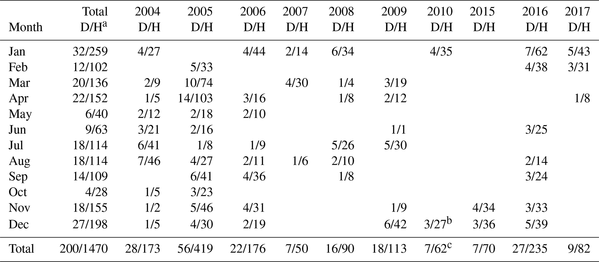
a D/H stands for days and hours. b Observed in 2003. c Including the observations in 2003.
The potential energy density Ep can be estimated from temperature observations and then is chosen as a measure of GW activity. Ep is defined as (see, e.g., Vincent et al., 1997)
where
Here, g is equal to 9.5 ms−2, which is the gravitational acceleration in the MLT; N is the Brunt–Väisälä frequency calculated according to Eq. (2); is the mean temperature averaging over altitude; T′ is the temperature perturbation; and Cp is the constant-pressure heat capacity, equal to 1004 J K−1 kg−1. In Eq. (1), the calculation of Ep depends on the estimations of N, , and T′. The procedure adopted by Gardner and Liu (2007) is closely followed here for the estimation of T′. It includes four steps. Step 1: for the unified data with 0.9 km and 30 min in each night of observation, data points with photon noise errors larger than 10 K in temperature are discarded. Step 2: the linear trend in time at each altitude in the temperature profiles is then subtracted to eliminate the potential biases associated with GWs with periods longer than about twice the observation period. Step 3: deviations exceeding 3 standard deviations from the nightly mean are discarded from the resultant temperature deviation series at each altitude to remove occasional outliers. Step 4: the vertical mean is subtracted from each temperature deviation profile to eliminate the influences of the waves with vertical wave length longer than about twice the profile height range (∼25 km). The resultant temperature deviations (ΔT) are used to calculate nightly mean temperature perturbation ().
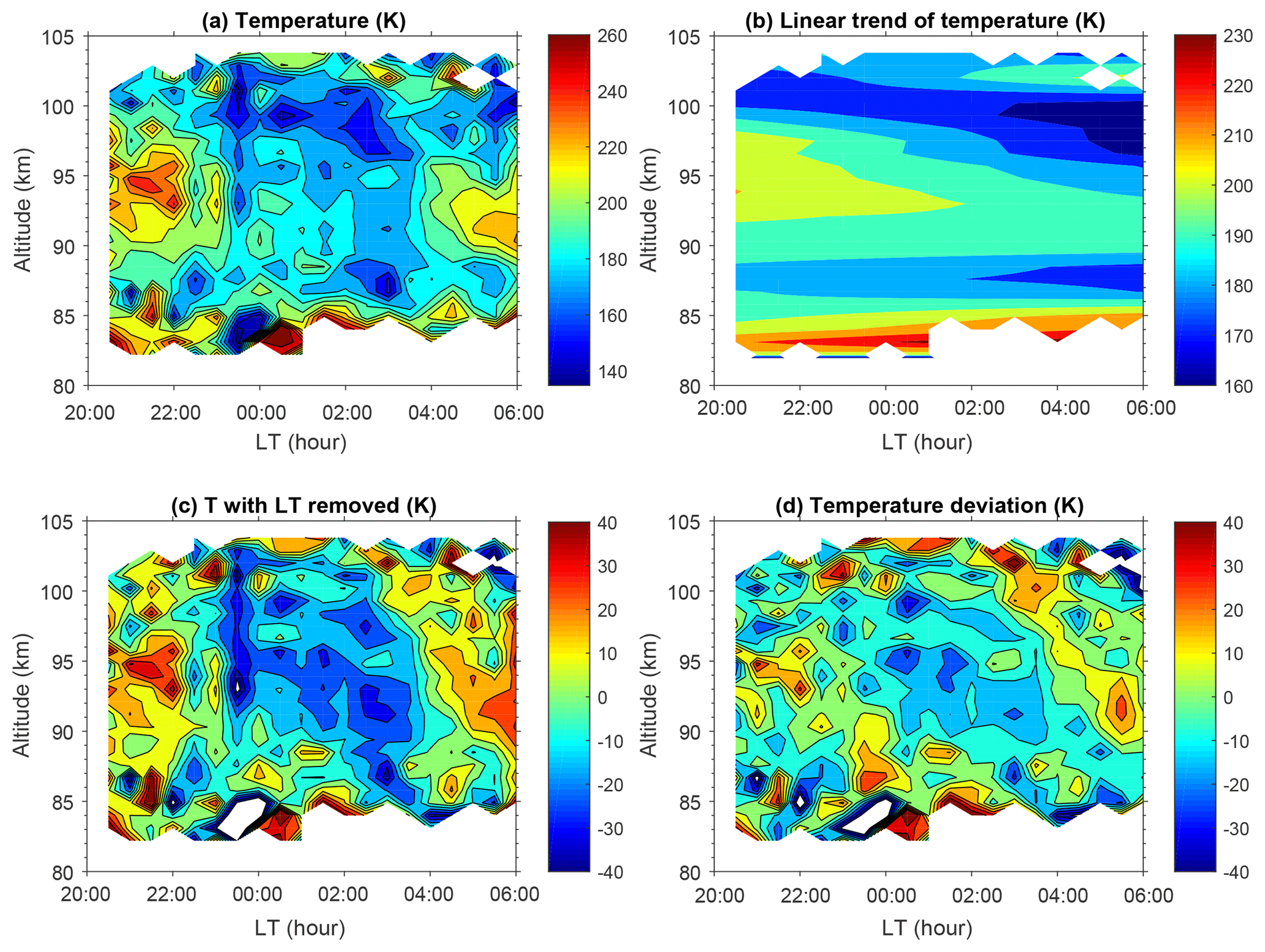
Figure 2Illustration of data processing for temperature on 18 December 2003: (a) K lidar-measured temperature with 0.9 km and 30 min vertical and temporal resolutions, respectively; (b) linear trend of temperature in time; (c) temperature perturbations after removing the linear trend in time; and (d) temperature perturbations after removing the linear trend in time and the vertical mean.
The data on 18 December 2003 are taken as an example of the data processing. Figure 2a shows the temperature contours after Step 1. The data largely cover the 82–103 km altitude range, and the bottom edge increases to about 84 km in the second half of the night. Figure 2b show the subtracted trends in time, which indicate that the background temperature decreases at each altitude in the 85–100 km range but increases near both the bottom and top edges. Figure 2c shows the corresponding temperature deviations. The temperature deviations after Step 4 are shown in Fig. 2d. It shows that, in contrast to midlatitudes and high latitudes (e.g., Baumgarten et al., 2018; Rauthe et al., 2008), the perturbations (GWs) are dominated by small-scale variability and to a smaller extent by coherent wave structures. The difference between Fig. 2c and d is pronounced. This indicates that Step 4 is effective in eliminating the influences of the waves with longer vertical wavelength. Furthermore, Guharay and Franke (2011) have given a rather strong semidiurnal tidal amplitude in the mesopause region through meteor radar observations over a nearby site (20.7∘ N, 156.4∘ W). The amplitude increases with altitude and shows a clear SAO pattern, with maxima during solstices. This kind of feature is not found in the variations of GWPE with altitude and season in later sections of this paper. However, the total effectiveness of this method in removing the tidal amplitude is not easy to evaluate due to the lack of knowledge on tidal components at this latitude and the shorter and often intermittent measurement periods.
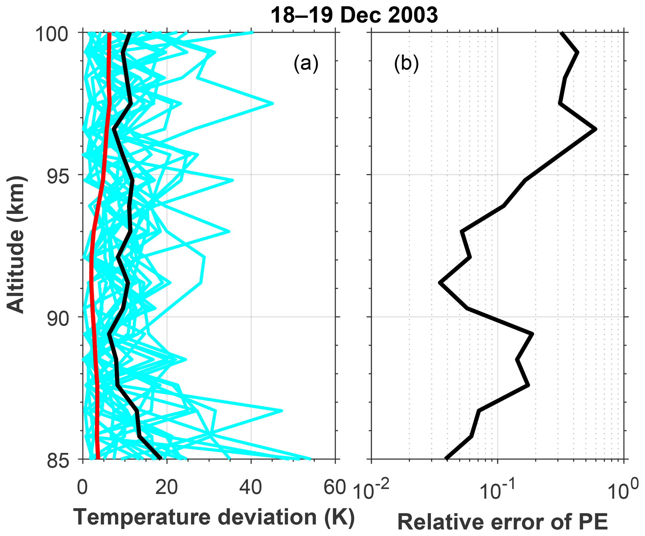
Figure 3(a) Individual temperature deviation profiles on 18–19 December 2003. In addition, the mean statistical uncertainties of the measurements (red solid line) and the mean fluctuations at every altitude (black solid line) are shown. (b) Relative error of potential energy at every altitude due to statistical uncertainty in the temperature measurements.
Figure 3a shows the individual profiles of the temperature fluctuations (cyan curves) for the night. The nightly mean temperature perturbations and the statistical uncertainties are also presented by black and red lines, respectively. The statistical uncertainties are usually less than 5 K below 95 km altitude, and they increase a bit to ∼6 K and remain above, while the nightly mean temperature perturbations decrease from ∼18 K at 85 km to ∼6 K at 89.5 km and then increase to and oscillate near 11 K above. The square of the ratio of temperature statistical uncertainty over nightly mean perturbation is plotted in Fig. 3b. It represents the relative error in estimating the potential energy due to statistical uncertainty in the temperature data. In this night, the relative errors are lower than 20 % below 95 km and become larger above. The maximal relative error occurs just below 97 km with a value of 59 %. The relative error is a bit larger than 30 % near 100 km altitude but less than 10 % near 85 km.
The unified 0.9 km and 30 min resolution temperature profiles in each observational night in the same composite week are binned and averaged to the fixed vertical and temporal grids to construct the weekly composite night of temperature of a year.
The weekly composite night data of are first spatially smoothed and then temporally smoothed using Hamming windows with a full width at half maximum (FWHM) of 2.7 km and 3 h, respectively. This method of computing the weekly composite night follows the approach used by Friedman and Chu (2007) and the references therein. The resulting weekly composite night of temperature usually covers most of the night from sunset to sunrise (not shown here; the resulting monthly composite night can be seen in Fig. 3 of Friedman and Chu, 2007, which is computed with a small part of the dataset used here). It is a close representation of the mean state at the fixed time and altitude bins within an average weeknight. After that, the weekly composite nights are then averaged to derive the weekly mean profiles. The nightly mean temperature perturbation profiles with unified 0.9 km resolution in the same composite week are averaged to obtain the weekly mean temperature perturbation profile. The weekly mean profiles of N2 and the consequential Ep at 0.9 km resolutions are estimated using Eqs. (2) and (1), respectively. For the weekly mean profiles of each parameter, they are fitted to a harmonic fit model including the annual mean plus 12-month (annual) oscillation and 6-month (semiannual) oscillation. The equation of the model is as follows:
where Ψ(zt) is the value of a weekly mean parameter at altitude z and week t, expressed in week of the year (1–52); Ψ0(z) is the annual mean; and An(z) and φn(z) () are the amplitude and phase of the n-month oscillation, respectively.
To keep the characteristics of higher-order components in the seasonal climatology of each parameter, the fitted Ψ(z,t) was subtracted from the raw weekly mean profiles and the residuals were smoothed using a Hamming window with a FWHM of 4 weeks. The smoothed residuals were then added back to the fitted Ψ(z,t); the resulting seasonal climatology (hereafter SC) of each parameter is illustrated together with weekly mean profiles in the Results section. Meanwhile, the fitted seasonal variations (hereafter SV) Ψ(z,t) of each parameter, i.e., the mean plus the annual and semiannual harmonic fits, are also presented together with the amplitude and phase information of each monochromatic wave in the following section.
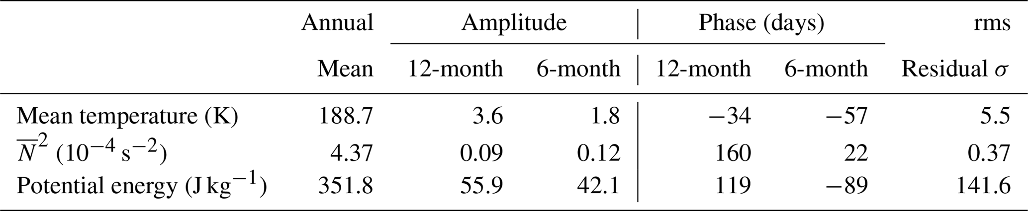
In the following the results of the analysis are shown and discussed with respect to the seasonal variation of the mean temperature (Sect. 4.1), the square of the Brunt–Väisälä frequency (Sect. 4.2), and the GW activity (Sect. 4.3). Therefore, we plot the weekly mean profiles and the corresponding SCs of , N2, and Ep in Figs. 4, 6, and 8, respectively, at 0.9 km vertical and 1-week temporal intervals. The SVs of , N2, and Ep by applying Eq. (2) are presented in Figs. 5a, 7a, and 9a, respectively. The amplitudes and phases of the 12-month and 6-month oscillations of the regression model are plotted in Figs. 5c, 7c and 9c and 5d, 7d and 9d, respectively. In the raw data, temperature error due to photon noise is usually less than 5 K in the 87–97 km altitude range because the K density in this range is usually much larger (e.g., Yue et al., 2017). To show the seasonal variation of each parameter more clearly, the data between 87 and 97 km are averaged by altitude and then fitted to the same seasonal model consisting of the annual mean, AO, and SAO. Note that it is a risk to smooth the temporal variations for those parameters, such as N2, which strongly vary in terms of altitude in this range. The averaged results and the fitted curves are plotted in Figs. 5b, 7b and 9b. The statistical parameters for these fits are summarized in Table 2.
Table 2Parameters of mean temperature, temperature variance, squared Brunt–Väisälä frequency, and potential energy averaged between 87 and 97 km.
4.1 Seasonal variation of the mean temperature
The weekly mean temperature illustrated in Fig. 4a and the SC of temperature illustrated in Fig. 4b show that the Arecibo climatology is warmer in late autumn and early winter and colder in summer at all altitudes. Figure 5a shows the seasonal variation of temperature synoptically. Temperature inversion layers (TILs) are present most of the time. The altitudes at which the temperature gradient changes from positive to negative are represented by the black crosses in both Figs. 4b and 5a. The deviations of TILs between these two figures are minor most of the time. Significant differences mainly occur in the period between September and December. The inversion layers near 92 km in late September and near 89 km from late November to early December in Fig. 4b vanish in Fig. 5a; meanwhile, the inversion layer near 94 km during the first half of September changes to ∼92 km in Fig. 5a. It is noted that the temperatures vary slightly from 85 to 94 km altitude most of the time from September to December. The inversion layers, evaluated by finding the zero value of the temperature gradient, are not statistically significant in this period. Therefore, we ignore the period from September to December when discussing the TILs. However, there is a common feature of a temperature maximum at ∼97 km in October and November in both Figs. 4b and 5a. To simplify the analysis of the influences of different harmonic components, we take Fig. 5a as an example in the following descriptions and discussions. In spring, TILs occur at ∼96 km from late February to April. In summer, TILs appear at ∼91 km from late May to the first half of September. In winter, TILs occur at ∼94 km from January to the first half of February. The minimal temperature occurs near 98.5 km most of the time except for the period from the second half of September to November, when it is situated at ∼96 km. This should correspond to the mesopause according to the result that the mesopause is at the 95–100 km level at low latitudes obtained by SABER observations (Xu et al., 2007a).
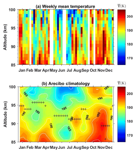
Figure 4(a) The weekly mean temperature profiles in the mesopause region at Arecibo. (b) Temperature climatology obtained by first applying a harmonic fit to the data shown in (a) and adding the residuals smoothed by using a hamming window with lengths of 4 weeks in time and 2.7 km in vertical dimension.
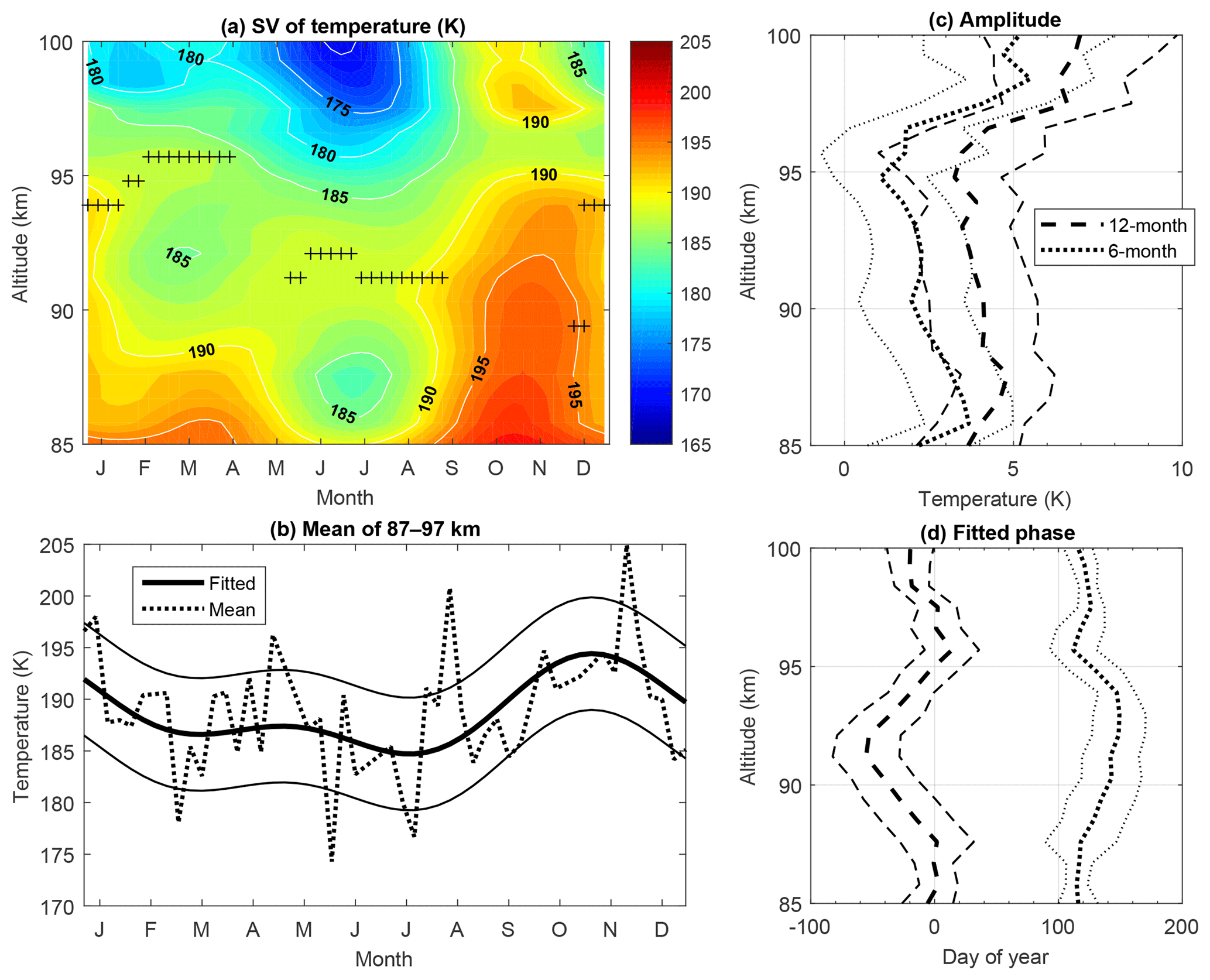
Figure 5(a) Seasonal variations of the harmonic fitted nocturnal temperature plotted versus altitude and month, where the crosses represent the altitude of temperature inversion layer. (b) Observed (dotted curve) and harmonic fitted (thick solid curve) mean temperature between 87 and 97 km, where the width between the thin solid curves and the thick solid curve is 1 standard deviation (1σ). (c) 12-month (dashed curve) and 6-month (dotted curve) amplitudes and their 1σ deviations (thin lines). (d) 12-month (solid curve) and 6-month (dotted curve) phases and their 1σ deviations (thin lines).
Figure 5c shows that the amplitudes of the AO are obviously larger than that of the SAO. Figure 5d shows that the phase (defined as the time of the maximum perturbation) of AO oscillates in the range between the day of year (DOY) −60 and 10, while that of SAO varies between DOY 110 and 150. Figure 5b shows that the mean temperature is warmest between October and November and coldest in July. A secondary peak/trough occurs in April/February.
Notice that the warmest temperature occurs around October with the shortest observation times, which reduce the confidence level of the harmonic fit. However, the observation times in both September and November are longer than 100 h in more than 10 nights; they help to keep the confidence level of the harmonic fit. Moreover, the temperature structure shown in Fig. 5a agrees well with the temporal variations of the equatorial zonal mean temperature in the range 85–100 km observed by SABER (Xu et al., 2007b). The amplitudes and phases of both SAO and AO observed by SABER at 20∘ N latitude were shown by Xu et al. (2007b) in the middle panels of their Fig. 10. Comparisons show that the lidar-observed phases of both SAO and AO shown in Fig. 5d agree with those obtained by SABER in the same altitude range. The SAO amplitude shown in Fig. 5c agrees quite well with that observed by SABER in both magnitude and vertical structure. The lidar AO amplitude shows similar vertical structure with that of SABER, but the magnitude of lidar AO amplitude is at least 1 K larger than that observed by SABER. The agreement between lidar and SABER observations gives us more confidence to use the lidar-observed temperature data in studying the GW activities in latter sections.
Except for the smaller amplitude of SAO oscillation in this study, the phase of SAO and the amplitude and phase of AO of the mean temperature are consistent with a previous study by Friedman and Chu (2007) (see their Figs. 6 and 7), who used data collected between December 2003 and September 2006. Comparing Fig. 4b here to Fig. 6 in Friedman and Chu (2007), there are some different features in these two climatology results. For example, the temperatures are about 10 K warmer in the winter months of December and January in this study. The differences are caused by two reasons. The first reason is the much more extensive dataset from the year 2003 to 2017, covering a whole solar period here. The second reason is that the harmonic fit model is applied to weekly averages here, while it was applied to monthly averages in Friedman and Chu (2007).
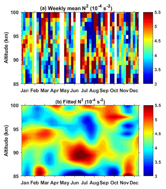
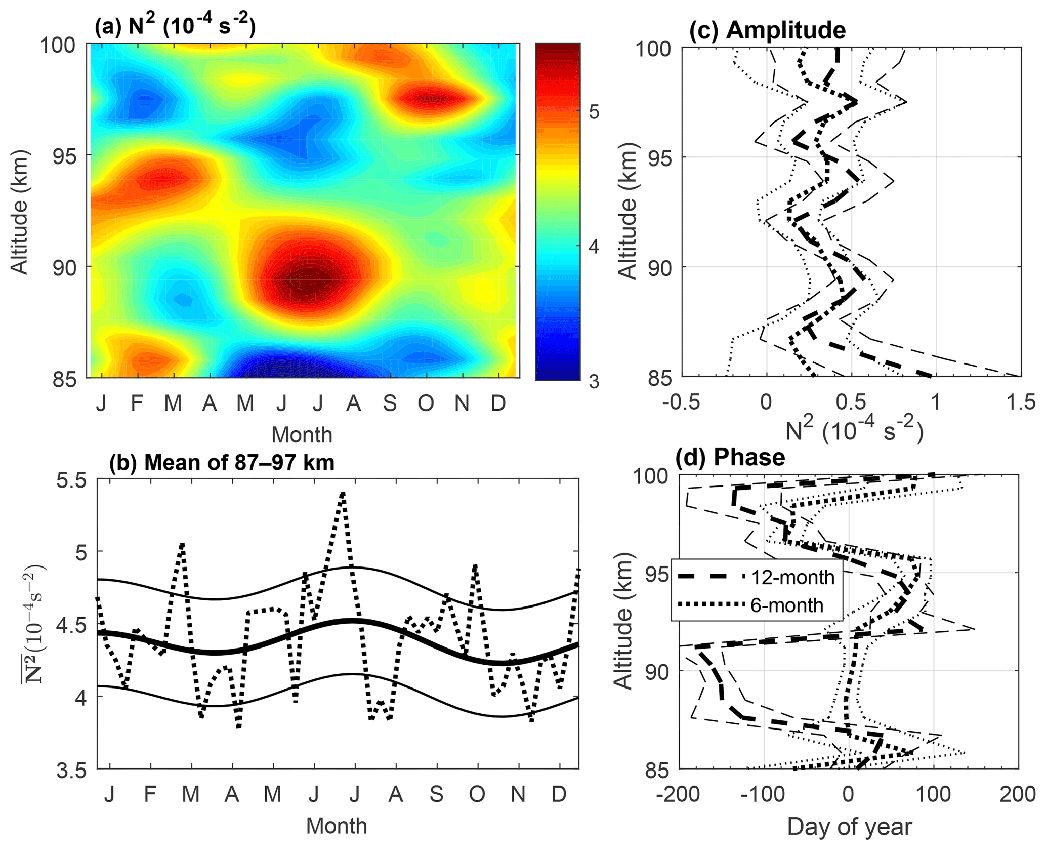
Figure 7(a) Seasonal variations of the harmonic fitted squared Brunt–Väisälä frequency N2 plotted versus altitude and month. (b) Observed (dotted curve) and harmonic fitted (thick solid curve) mean N2 between 87 and 97 km, where the width between the thin solid curves and the thick solid curve is 1σ. (c) 12-month (thick dashed curve) and 6-month (thick dotted curve) amplitudes and their 1σ deviations (thin lines). (d) 12-month (thick dashed curve) and 6-month (thick dotted curve) phases and their 1σ deviations (thin lines).
4.2 Square of the Brunt–Väisälä frequency
The square of the Brunt–Väisälä frequency N2 is a good indicator to characterize the atmospheric static stability. Gardner and Liu (2007) indicated that the resulting N2 was usually overestimated in this way due to the eliminations of gravity waves when the weekly mean temperature profiles were derived by employing data averaging. However, they pointed out that the lower-value regions of N2 represented the lower stability of the atmosphere well, i.e., the greater wave dissipations. Figures 6 and 7a show that N2 is highly variable with season and altitude. Taking the summer months from June to August as an example, Fig. 7a shows that N2 is quite low near the bottom and then increases quickly with altitude. It is obviously large between altitudes of 87 and 92 km and decreases above. It is small in the 94–98 km range and starts to increase gradually near the top boundary. The seasonal variations are obviously different every 4 km at altitudes from 87 to 96 km. The features shown in Fig. 6b are more complicated than Fig. 7a. Assuming an isothermal atmosphere with the background temperature being 190 K, N2 is estimated to be about s−2, which is largely represented by the orange color in Figs. 6b and 7a. Therefore, below about 96 km, the regions with a red color (larger than s−2, indicating a positive temperature gradient with altitude) agree with the TILs as expect. It shows clearly that the TILs occur at about 92–95 km altitude in February and March, while they occur at about 87–92 km altitude through the summer months. A low value of GWPE is expected in the region, with N2 being large in the case that other parameters keep unchanged.
The fitted curve of (average of N2 between 87 and 97 km height) as shown in Fig. 7b exhibits a seasonal variation. The maximum occurs in July and the minimum between October and November, while a secondary maximum occurs between January and February and a secondary minimum in May. However, it is noted that the seasonal variations of N2 vary highly with altitude. This 87–97 km mean fitting curve cannot represent the whole features of N2 in this altitude range.
Figure 7c shows that the amplitudes of the 12-month and the 6-month oscillations are comparable throughout most of the altitude range of interest. They oscillate similarly and look like sinusoids, with troughs occurring at altitudes ∼87, ∼92, ∼96, and ∼98 km. The phases of these two components illustrated in Fig. 7d also show a quick transition at these altitudes.
4.3 Seasonal variation of the gravity wave activity
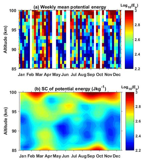
GW activity is directly manifested by the wave energy. Figure 9a shows the contour plots of the harmonic fitted GWPE Ep from lidar observations. Ep is colored on a logarithmic scale (log10). It can be seen that, below 97 km altitude, Ep always reaches the maximum in equinox seasons, and mostly near spring equinox. More interesting, in equinox seasons the potential energy decreases with altitude from the bottom to ∼91 km and then shifts to increase with altitude in the range from 91 to 95 km. However, the potential energy is quite smaller in the altitude range 85–95 km during solstices. The energies are low near 91 km throughout the year. Above 91 km and below 97 km, an obvious SAO is visible in Fig. 9a. The oscillations of potential energy become very weak around 97 km. The SC of potential energy illustrated in Fig. 8b shows some difference. The seasonal variations of Ep exhibit an oscillation with a period of ∼3 months at 87–95 km altitude. A dominant maximum occurs from the second half of March to the first half of April. Several minima occur in January–February, May–June, August–September, and November–December. This implies that some higher-order oscillation may also play an important role besides the AO and SAO. We note this feature of Ep varying with a higher oscillation pattern and leave it for further discussion. We only focus on AO and SAO in this paper.
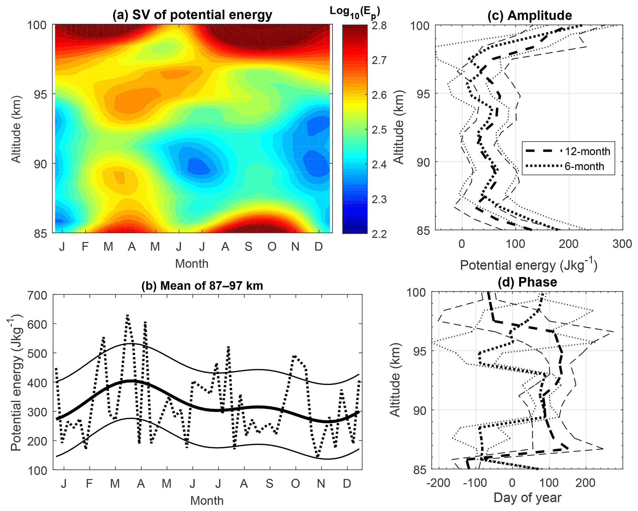
Figure 9(a) Seasonal variations of the harmonic fitted potential energies plotted versus altitude and month. (b) Observed (dotted curve) and harmonic fitted (thick solid curve) mean potential energy between 87 and 97 km, where the width between the thin solid curves and the thick solid curve is 1σ. (c) 12-month (thick dashed line) and 6-month (thick dotted line) amplitudes and their 1σ deviations (thin lines). (d) 12-month (thick dashed line) and 6-month (thick dotted line) phases and their 1σ deviations (thin lines).
Figure 9c shows that the amplitudes of both the 12-month and the 6-month oscillations are comparable at most altitudes. The amplitude of SAO becomes smaller in the altitude range 94–98 km. It decreases to almost 0 J kg−1 at 97–98 km. Figure 9d shows that the phase of SAO is almost independent of altitude. It is quite close to DOY 100 at most altitudes. The AO almost has the same phase as the SAO from 88 to 96 km altitude. Its phase shifts to the end of the year near the top edge, where the dominant seasonal variation is evident.
In the altitude range 87–97 km, Fig. 9c shows that the amplitudes of both AO and SAO vary slightly; meanwhile, Fig. 9d shows that the phases of both AO and SAO also vary slightly. Therefore, the mean Ep averaged in the altitude range 87–97 km and the corresponding harmonic fit shown in Fig. 9b can represent the seasonal behavior of Ep in this altitude range well. The harmonic fit curve of Ep shows a combination of AO and SAO, with a maximum of 404 J kg−1 near the vernal equinox and a minimum of 264 J kg−1 at the end of November. The maximum is a factor of 1.5 larger than the minimum.
5.1 Mesospheric temperature inversion layer
We have noticed that obvious TILs occur at ∼96 km in spring, at ∼91 km in summer, and at ∼92 km in early autumn. The TILs in the upper mesosphere over Arecibo were reported both in a case study and a study of climatology by using a subset of the data used in this study (Yue et al., 2016; Friedman and Chu, 2007). The formation mechanism for TIL in the mesopause region was reviewed by Meriwether and Gerrard (2004). One primary mechanism for the upper mesosphere TIL is that upward propagating GWs reach a critical level via interaction with the background flow and/or tides. The GWPE accumulates with the wave compressed in reaching to the critical level. Xu et al. (2009) analyzed satellite observations and showed that the DW1 tide interacted with GWs, leading to the damping of both the DW1 tide and GWs; the larger the amplitude of DW1, the larger the damping. Consequently, the occurrence of TIL and the decrease of the GW Ep are expected at and just below the locations where the DW1 amplitude is large. The climatology of WACCM simulations showed that, at 20∘ N, both the zonal and meridional components of DW1 tide amplitudes are large in the height range 80–100 km around the vernal equinox and in the altitude range 90–100 km in summer months from June to August (e.g., Fig. 10 in Smith, 2012). These areas with large DW1 tide amplitude in Fig. 10 of Smith (2012) match perfectly with the TILs in Fig. 5a.
5.2 Reduction of GWPE
For freely propagating GWs, the potential energy per unit mass (J kg−1) should increase exponentially with altitude for the conservation of energy. Figure 9a shows that the potential energy decreases first and then starts to increase gradually with altitude below ∼97 km in all seasons. Above ∼97 km, the GWPE enhanced significantly with altitude. This behavior of mean potential energy is quite similar to that retrieved from satellite temperature data (Offermann et al., 2006; see their Figs. 10 and 11). The altitude of ∼97 km is in the vicinity of their wave turbopause altitude range, is close to the mesopause over this site (Friedman and Chu, 2007; Xu et al., 2007a; Yue et al., 2017), and is the level at which the seasonal variation of zonal winds changing from a clear SAO pattern to a AO dominant pattern is evident (e.g., Li et al., 2012). This result suggests a possible mechanism for the GW energy dissipation; i.e., the GW dissipates or deposes energy or momentum below about the mesopause (or the wave turbopause defined by Offermann et al., 2006). This conjecture should be taken with caution because the relative error in the estimated Ep could reach 30 % or even larger due to the statistical uncertainty of temperature measurement in this altitude range. But the quantitative influence of this uncertainty on the energy increase with altitude is hard to evaluate because the statistical uncertainty does not show an increase trend in the 96–100 km altitude range as shown in Fig. 3b. In addition, it needs to be pointed out that the increasing Ep above 97 km in spring, autumn, and winter months matches with the increasing easterly winds in this altitude range and seasons as discussed in Sect. 5.3.
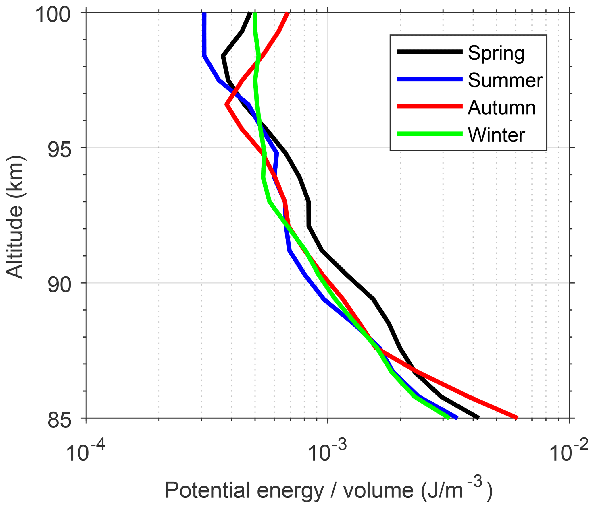
Figure 10Vertical profiles of the potential energy per unit volume (in J m−3) averaged over spring (13 weeks mean centered at vernal equinox, shown by the black line), summer (13 weeks mean centered at summer solstice, shown by the blue line), autumn (13 weeks mean centered at autumn equinox, shown by the red line), and winter (13 weeks mean centered at winter solstice, shown by the green line).
To learn in depth the dissipation of GWs in the mesopause region at Arecibo, we multiplied the harmonic fitted Ep by the air density taken from the CIRA-86 reference atmosphere (Fleming et al., 1990) and averaged the weekly profiles every 13 weeks (period of a season), centering at each equinox or solstice. The resultant profiles of the potential energy per unit volume (in J m−3) in four seasons are plotted in Fig. 10. If GWs propagate upward without energy dissipation, the lines of energy per unit volume would be vertical. Therefore, the overall left-sloping lines in Fig. 10 indicate that the reductions of GWPE occur below ∼97 km in all seasons. The reduction of GWPE in the mesosphere has been reported by lidar observations at other latitude stations (e.g., Mzé et al., 2014; Rauthe et al., 2008). Both observations of Mzé et al. (2014) and Rauthe et al. (2008) indicated dissipation of GW Ep throughout the mesosphere in all seasons.
The reduction of GW Ep indicates the deposition of GW energy and momentum into the background atmosphere, which would lead to the increase of background temperature and/or even the occurrence of TIL. This drives us to investigate the relationship between the reduction of GW Ep and the temperature structure in depth. We are excited to find that each profile of the GWPE per unit volume (in J m−3) as shown in Fig. 10 shows a more rapid reduction of energy at and below the TIL altitude of the corresponding season and changes to a much slower reduction and/or even conservation of energy above, for example, the behaviors of the green curve (profile for winter) around 94 km altitude (the altitude of TILs in winter), the blue curve (profile for summer) around 91 km altitude (the altitude of TILs in summer), and the black curve (profile for spring) around 97–98 km altitude (∼1 km above the altitude of TILs in spring). These close connections of the mesospheric TILs with the reduction of GWPE provide strong support for the mechanism that the upper mesosphere TIL formed due to the interaction of GWs with the upper mesospheric wind or diurnal tides through critical-level effects. From another point of view, the strong gradient change in the seasonal mean profiles of GWPE per unit volume should be induced strongly by the horizontal wind field in this region.
5.3 Seasonal variations of GWPE
We point out a semiannual cycle of GW Ep, with a maximum in spring and a minimum in summer and a second maximum in autumn and a second minimum in winter in the altitude range 87–97 km. The maximum of the GW Ep alters in autumn to below 87 and above 97 km altitude. These results agree with the observations at other low-latitude stations. Gavrilov et al. (2003) studied the GW seasonal variations by using medium-frequency (MF) radar observation over Hawaii (22∘ N, 160∘ W). They found a semiannual variation of GWs with the maximum intensity at the equinoxes above 83 km; the mean zonal wind also had a mainly semiannual variation in this altitude range. The seasonal variations of GW activities at low-latitude stations are different to those obtained from lidar observations at other latitude stations in the upper mesosphere (Mzé et al., 2014; Rauthe et al., 2006, 2008). Rauthes et al. (2008) provided the seasonal variations of GW Ep at a station of 54∘ N latitude by using 6 years of lidar temperature observations from 1 to 105 km. They showed an annual-dominated variation of GW Ep, with a maximum in winter and a minimum in summer in the mesopause region. Mzé et al. (2014) reported a semiannual variation of GW Ep, with maxima in winter and in summer and minima during the equinoxes in the upper mesosphere (∼75.5 km), by using Rayleigh lidar observations from 1996 to 2012 at a midlatitude station (∼44∘ N). They showed that the maximum of Ep was about 144 J kg−1 on average at 75.5 km in August, while the minimum of Ep is about a factor of 2.5 smaller than the maximum. The ratio between the maximum and the minimum is obviously larger than that of 1.5 in the altitude range 87–97 km at Arecibo.
The cause of the observed seasonal variations of GW activities in the mesosphere was discussed by several authors. One that is often of concern is the influence of critical level filtering of GWs by the background wind (Lindzen, 1981; Yue et al., 2005). Gavrilov et al. (2003) attributed their observed semiannual variation of GW intensity to the dependence of GW generation and propagation on the background wind and temperature through numerical simulations. At a midlatitude station, Juliusruh (55∘ N, 13∘ E), Hoffmann et al. (2010) reported semiannual variations of GW activity in the upper mesosphere and lower thermosphere, with maxima in winter and summer and minima during equinoxes by using MF-radar-measured winds. This seasonal dependence is assumed to be mainly due to the filtering of GWs by the background wind in the stratosphere and lower mesosphere. This is not always the case. Rauthe et al. (2008) did not find a direct correlation between the strength of the GW activity and the background wind direction and/or wind speed taken from the European Centre for Medium-Range Weather Forecasts analysis.
Here we also want to check the relation between our observed GW activity and the wind direction and/or wind speed. Some scientific literature reported studies about the seasonal variation of mean zonal wind in the tropical mesopause region (see, e.g., Fig. 3 in Garcia et al., 1997; Fig. 1 in Li et al., 2012; and Fig. 3 in Smith, 2012). The monthly mean HRDI equatorial zonal wind showed that easterly winds were prevailing in equinox seasons near 80 km altitude. They then decreased with altitude from 80 km above and started to increase above ∼92 km, while the westerly winds prevailed in the range 80–94 km in solstice seasons; then the easterly winds prevailed. The reversal is at about 95 km (Smith, 2012). The zonal winds observed by meteor radar at a nearby site, Maui (20.7∘ N, 156.4∘ W; see Fig. 1a in Li et al., 2012), showed further that the westerly winds prevailed throughout the 80–100 km altitude range in the summer months from May to August. This provides us the opportunity to compare our GW Ep climatology shown in Fig. 9a with the mean zonal wind climatology shown in Fig. 1a of Li et al. (2012) or the upper panel of Fig. 3 in Smith (2012) season to season and altitude to altitude. Here we focus on the altitude range 85–100 km.
Firstly, the mean zonal winds have a dominant SAO, with westerly winds prevailing in solstice seasons and easterly winds (or weak westerly winds) prevailing in equinox seasons; meanwhile, our GW Ep has a SAO, with minima in winter and summer and maxima during equinoxes. Secondly, the easterly winds are much larger (or the westerly winds are much smaller) in the altitude range 85–95 km around the vernal equinox than around the autumn equinox, which corresponds to the fact that the magnitude of GW Ep in spring is significantly greater than that in autumn. This correlation is also verified by the fitted curve in Fig. 9b. The maximum of Ep at the vernal equinox with a value of 404 J kg−1 is a factor of 1.3 larger than the second maximum of 319 J kg−1 at the autumn equinox. Thirdly, the largest westerly winds near 90 km in June match perfectly with the minimal Ep at almost the same altitude and at almost the same time. Fourthly, the decrease of easterly winds with altitude near 85 km during equinoxes is in accordance with the strong but decreasing GW Ep with altitude in almost the same altitude range and seasons. Fifthly, the transition of mean zonal winds from decreasing westerly winds to increasing easterly winds above 96 km before middle April and after July corresponds well with the increasing Ep in the same altitude range and seasons. These five features provide strong evidence of an indeed pronounced correlation between the local mean zonal wind field and the lidar-observed GW Ep. This correlation agrees perfectly with the connection of wind and GWs in the middle atmosphere demonstrated by Lindzen (1981). It means that the seasonal variations of the GW activity in the MLT region at this site are determined by the selective filtering of GWs by the strong tropical zonal wind SAO in the same region.
It is noted that the GWPE increases instead of being constant with altitude as expected for freely propagating linear waves above 98 km in spring and above 96 km in autumn as shown in Figs. 10 and 9a. We notice that the corresponding regions of increasing GWPE enhancement with altitude in Fig. 9a are clearly associated with regions of increasing zonal wind shears (in magnitude) in Fig. 1a and b of Li et al. (2012), which suggests that conversion of energy contained in the mean wind into the energy of perturbation due to the increasing dynamical instability should be an important mechanism for the enhancement of GWPE near 100 km altitude in equinox seasons.
The first complete range-resolved climatology of potential energy in the tropical mesopause region is present using 11-year-long nocturnal temperature measurements by the K Doppler lidar over the Arecibo Observatory. The mean temperature , the square of the Brunt–Väisälä frequency N2, and the potential energy of perturbation associated with GWs are estimated with high accuracy and resolution from the temperature data. The main characteristics of the observations are as follows.
-
Mesospheric TILs occur in the altitude range 90–95 km in most months except from September to December.
-
The GWPE per unit volume (in J m−3) reduces in the altitude range 85–97 km in all seasons. A close relationship exists between the reduction of GWPE and the TILs. This provides strong support for the mechanism of the TIL formation in the mesopause region.
-
The seasonal variations of GWPE show clear SAO at most altitudes. The maxima occur in spring and autumn, and the minima occur during solstices. AO and some higher-order oscillations still play important roles. The harmonic fitted GWPE with the annual mean plus the AO and SAO is compared to the MLT wind field in the tropical region as published by Li et al. (2012) and Smith (2012); there is indeed a pronounced altitudinal and temporal correlation between them. This suggests that the seasonal variation of GW activity should mainly be determined by the local wind field through the influence of critical level filtering of GWs by the background wind.
-
The GWPE increases near 100 km altitude in equinox seasons instead of being constant with altitude as expected for freely propagating linear waves. This was most possibly caused by the conversion of energy contained in the mean wind into the energy of perturbation due to dynamical instability.
The National Astronomy and Ionosphere Center (NAIC) Arecibo Observatory (AO) is a national facility operated by the University of Central Florida that provides upper atmospheric observing capabilities to the broader scientific community. Data from its observations are disseminated through the NAIC website (http://www.naic.edu/aisr/database/html/framedoc.html, Arecibo Observatory, 2001, Lidar [K], last access: June 2012), and the Madrigal Database at the Haystack Observatory (http://millstonehill.haystack.mit.edu/list/, Haystack Observatory, 2003).
XY conceived the idea. JSF and JL conducted the observations. XY processed the experimental data and performed the analysis. XY, QZ, JSF, and XW contributed to the interpretation of the results. XY wrote the manuscript with support from QZ, JSF, and JL. All authors provided critical feedback and helped to improve the manuscript.
The authors declare that they have no conflict of interest.
This article is part of the special issue “Layered phenomena in the mesopause region (ACP/AMT inter-journal SI)”. It is not associated with a conference.
The study is supported by NSFC grants 41474128 and 61771352 and NSF grant AGS-1744033. The Arecibo Observatory is operated by
the University of Central Florida under a cooperative agreement with the
National Science Foundation (AST-1744119) and in alliance with Yang
Enterprises and Ana G. Méndez-Universidad Metropolitana. The authors
thank John Anthony Smith, Frank Djuth, Dave Hysell, Min-Chang Lee, and Eframir Franco Diaz for their help with the observations. In
addition, we are grateful to the two anonymous reviewers and the editor Robert Hibbins for improving the paper with their helpful comments.
Edited by: Robert Hibbins
Reviewed by: two anonymous referees
Baumgarten, G., Fiedler, J., Hildebrand, J., and Lübken, F.-J.: Inertia gravity wave in the stratosphere and mesosphere observed by Doppler wind and temperature lidar, Geophys. Res. Lett., 42, 10929–10936, https://doi.org/10.1002/2015GL066991, 2015.
Baumgarten, K., Gerding, M., and Lübken, F.-J.: Seasonal variation of gravity wave parameters using different filter methods with daylight lidar measurements at midlatitudes, J. Geophys. Res.-Atmos., 122, 2683–2695, https://doi.org/10.1002/2016JD025916, 2017.
Baumgarten, K., Gerding, M., Baumgarten, G., and Lübken, F.-J.: Temporal variability of tidal and gravity waves during a record long 10-day continuous lidar sounding, Atmos. Chem. Phys., 18, 371–384, https://doi.org/10.5194/acp-18-371-2018, 2018.
Cai, X., Yuan, T., Zhao, Y., Pautet, P. D., Taylor, M. J., and Pendleton Jr., W. R.: A coordinated investigation of the gravity wave breaking and the associated dynamical instability by a Na lidar and an Advanced Mesosphere Temperature Mapper over Logan, UT (41.7∘ N, 111.8∘ W), J. Geophys. Res.-Space, 119, 6852–6864, https://doi.org/10.1002/2014JA020131, 2014.
Chane-Ming, F., Molinaro, F., Leveau, J., Keckhut, P., and Hauchecorne, A.: Analysis of gravity waves in the tropical middle atmosphere over La Reunion Island (21∘ S, 55∘ E) with lidar using wavelet techniques, Ann. Geophys., 18, 485–498, https://doi.org/10.1007/s00585-000-0485-0, 2000.
Dunkerton, T. J.: Theory of the Mesopause Semiannual Oscillation, J. Atmos. Sci., 39, 2681–2690, 1982.
Fleming, E. L., Chandra, S., Barnett, J. J., and Corney, M.: Zonal mean temperature, pressure, zonal wind, and geopotential height as functions of latitude, COSPAR international reference atmosphere: 1986, Part II: Middle atmosphere models, Adv. Space Res., 10, 11–59, https://doi.org/10.1016/0273-1177(90)90386-E, 1990.
Friedman, J. S. and Chu, X.: Nocturnal temperature structure in the mesopause region over the Arecibo Observatory (18.35∘ N, 66.75∘ W): Seasonal variations, J. Geophys. Res.-Atmos., 112, D14107, https://doi.org/10.1029/2006JD008220, 2007.
Friedman, J. S., Tepley, C. A., Raizada, S., Zhou, Q. H., Hedin, J., and Delgado, R.: Potassium Doppler-resonance lidar for the study of the mesosphere and lower thermosphere at the Arecibo Observatory, J. Atmos. Sol.-Terr. Phys., 65, 1411–1424, 2003.
Fritts, D. C. and Alexander, M. J.: Gravity wave dynamics and effects in the middle atmosphere, Rev. Geophys., 41, 1003, https://doi.org/10.1029/2001RG000106, 2003.
Garcia, R. R., Dunkerton, T. J., Lieberman, R. S., and Vincent, R. A.: Climatology of the semiannual oscillation of the tropical middle atmosphere, J. Geophys. Res.-Atmos., 102, 26019–26032, https://doi.org/10.1029/97JD00207, 1997.
Gardner, C. S. and Liu, A. Z.: Seasonal variations of the vertical fluxes of heat and horizontal momentum in the mesopause region at Starfire Optical Range, New Mexico, J. Geophys. Res.-Atmos., 112, D09113, https://doi.org/10.1029/2005JD006179, 2007.
Gardner, C. S. and Liu, A. Z.: Wave-induced transport of atmospheric constituents and its effect on the mesospheric Na layer, J. Geophys. Res.-Atmos., 115, D20302, https://doi.org/10.1029/2010JD014140, 2010.
Gavrilov, N. M., Riggin, D. M., and Fritts, D. C.: Medium-frequency radar studies of gravity-wave seasonal variations over Hawaii (22∘ N, 160∘ W), J. Geophys. Res., 108, 4655, https://doi.org/10.1029/2002JD003131, 2003.
Geller, M., Alexander, M. J., Love, P. T., Bacmeister, J., Ern, M., Hertzog, A., Manzini, E., Preusse, P., Sato, K., Scaife, A., and Zhou, T.: A comparison between gravity wave momentum fluxes in observations and climate models, J. Clim., 26, 6383–6405, https://doi.org/10.1175/JCLI-D-12-00545.1, 2013.
Guharay, A. and Franke, S. J.: Characteristics of the semidiurnal tide in the MLT over Maui (20.75∘ N, 156.43∘ W) with meteor radar observations, J. Atmos. Sol.-Terr. Phys., 73, 678–685, https://doi.org/10.1016/j.jastp.2011.01.025, 2011.
Haystack Observatory: Arecibo Potassium [K] lidar experiment, http://millstonehill.haystack.mit.edu/list/ (last access: August 2017), 2003.
Hirota, I.: Observational evidence of the semiannual oscillation in the tropical middle atmosphere – A review, Pure Appl. Geophys., 118, 217–238, https://doi.org/10.1007/BF01586452, 1980.
Hoffmann, P., Becker, E., Singer, W., and Placke, M.: Seasonal variation of mesospheric waves at northern middle and high latitudes, J. Atmos. Sol.-Terr. Phys., 72, 1068–1079, https://doi.org/10.1016/j.jastp.2010.07.002, 2010.
Huang, K. M., Zhang, S. D., and Yi, F.: Reflection and transmission of atmospheric gravity waves in a stably sheared horizontal wind field, J. Geophys. Res., 115, D16103, https://doi.org/10.1029/2009JD012687, 2010.
Kim, Y. -J., Eckermann, S. D., and Chun, H.-Y.: An overview of the past, present and future of gravity-wave drag parameterization for numerical climate and weather prediction models, Atmos.-Ocean, 41, 65–98, https://doi.org/10.3137/ao.410105, 2003.
Li, T., Leblanc, T., McDermid, I. S., Wu, D. L., Dou, X., and Wang, S.: Seasonal and interannual variability of gravity wave activity revealed by long-term lidar observations over Mauna Loa Observatory, Hawaii, J. Geophys. Res.-Atmos., 115, D13103, https://doi.org/10.1029/2009JD013586, 2010.
Li, T., Liu, A. Z., Lu, X., Li, Z., Franke, S. J., Swenson, G. R., and Dou, X.: Meteor-radar observed mesospheric semi-annual oscillation (SAO) and quasi-biennial oscillation (QBO) over Maui, Hawaii, J. Geophys. Res. 117, D05130, https://doi.org/10.1029/2011JD016123, 2012.
Lieberman, R. S., Burrage, M. D., Gell, D. A., Hays, P. B., Marshall, A. R., Ortland, D. A., Skinner, W. R., Wu., D. L., Vincent, R. A., and Franke, S. J.: Zonal mean winds in the equatorial mesosphere and lower thermosphere observed by the High Resolution Doppler Imager, Geophys. Res. Lett., 20, 2849–2852, https://doi.org/10.1029/93GL03120, 1993.
Lindzen, R. S.: Turbulence and stress owing to gravity wave and tidal breakdown, J. Geophys. Res., 86, 9707–9714, https://doi.org/10.1029/JC086iC10p09707, 1981.
Liu, H.-L. and Meriwether, J. W.: Analysis of a temperature inversion event in the lower mesosphere, J. Geophys. Res., 109, D02S07, https://doi.org/10.1029/2002JD003026, 2004.
Lu, X., Liu, A. Z., Swenson, G. R., Li, T., Leblanc, T., and McDermid, I. S.: Gravity wave propagation and dissipation from the stratosphere to the lower thermosphere, J. Geophys. Res.-Atmos., 114, D11101, https://doi.org/10.1029/2008JD010112, 2009.
Meriwether, J. W. and Gerrard, A. J.: Mesosphere inversion layers and stratosphere temperature enhancements, Rev. Geophys., 42, RG3003, https://doi.org/10.1029/2003RG000133, 2004.
Mzé, N., Hauchecorne, A., Keckhut, P., and Thétis, M.: Vertical distribution of gravity wave potential energy from long-term Rayleigh lidar data at a northern middle-latitude site, J. Geophys. Res.-Atmos., 119, 12069–12083, https://doi.org/10.1002/2014JD022035, 2014.
Offermann, D., Jarisch, M., Oberheide, J., Gusev, O., Wohltmann, I., Russell III, J. M., and Mlynczak, M. G.: Global wave activity from upper stratosphere to lower thermosphere: A new turbopause concept, J. Atmos. Sol.-Terr. Phys., 68, 1709–1729, https://doi.org/10.1016/j.jastp.2006.01.013, 2006.
Picone, J. M., Hedin, A. E., Drob, D. P., and Aikin, A. C.: NRLMSISE-00 empirical model of the atmosphere: Statistical comparisons and scientific issues, J. Geophys. Res. Pt. A, 107, 1468, https://doi.org/10.1029/2002JA009430, 2002.
Rauthe, M., Gerding, M., and Lübken, F.-J.: Seasonal changes in gravity wave activity measured by lidars at mid-latitudes, Atmos. Chem. Phys., 8, 6775–6787, https://doi.org/10.5194/acp-8-6775-2008, 2008.
Sivakumar, V., Rao, P. B., and Bencherif, H.: Lidar observations of middle atmospheric gravity wave activity over a low-latitude site (Gadanki, 13.5∘ N, 79.2∘ E), Ann. Geophys., 24, 823–834, https://doi.org/10.5194/angeo-24-823-2006, 2006.
Smith, A.: Global Dynamics of the MLT, Surv. Geophys., 33, 1177–1230, https://doi.org/10.1007/s10712-012-9196-9 2012.
Vincent, R. A., Allen, S. J., and Eckermann, S. D.: Gravity-Wave Parameters in the Lower Stratosphere, in: Gravity Wave Processes, NATO ASI Series (Series I: Environmental Change), edited by: Hamilton, K., vol 50., Springer, Berlin, Heidelberg, https://doi.org/10.1007/978-3-642-60654-0_2, 1997.
Xu, J., Smith, A. K., Collins, R. L., and She, C.: Signature of an overturning gravity wave in the mesospheric sodium layer: Comparison of a nonlinear photochemical-dynamical model and lidar observations, J. Geophys. Res., 111, D17301, https://doi.org/10.1029/2005JD006749, 2006.
Xu, J., Smith, A. K., Yuan, W., Liu, H.-L., Wu, Q., Mlynczak, M. G., and Russell III, J. M.: Global structure and long-term variations of zonal mean temperature observed by TIMED/SABER, J. Geophys. Res., 112, D24106, https://doi.org/10.1029/2007JD008546, 2007a.
Xu, J., Liu, H.-L., Yuan, W., Smith, A. K., Roble, R. G., Mertens, C. J., Russell III, J. M., and Mlynczak, M. G.: Mesopause structure from Thermosphere, Ionosphere, Mesosphere, Energetics, and Dynamics (TIMED)/Sounding of the Atmosphere Using Broadband Emission Radiometry (SABER) observations, J. Geophys. Res., 112, D09102, https://doi.org/10.1029/2006JD007711, 2007b.
Xu, J., Smith, A. K., Liu, H.-L., Yuan, W., Wu, Q., Jiang, G., Mlynczak, M. G., and Russell III, J. M.: Estimation of the equivalent Rayleigh friction in mesosphere/lower thermosphere region from the migrating diurnal tides observed by TIMED, J. Geophys. Res., 114, D23103, https://doi.org/10.1029/2009JD012209, 2009.
Yiğit, E. and Medvedev, A. S.: Internal wave coupling processes in Earth's atmosphere, Adv. Space Res., 55, 983–1003, https://doi.org/10.1016/j.asr.2014.11.020, 2015.
Yuan, T., Heale, C. J., Snively, J. B., Cai, X., Pautet, P.-D., Fish, C., Zhao, Y., Taylor, M. J., Pendleton Jr., W. R., Wickwar, V., and Mitchell, N. J.: Evidence of dispersion and refraction of a spectrally broad gravity wave packet in the mesopause region observed by the Na lidar and Mesospheric Temperature Mapper above Logan, Utah, J. Geophys. Res.-Atmos., 121, 579–594, https://doi.org/10.1002/2015JD023685, 2016.
Yue, X. and Yi, F.: Propagation of gravity wave packet near critical level, Sci. China Ser. E, 48, 538–555, https://doi.org/10.1360/102005-24, 2005.
Yue, X., Zhou, Q., Raizada, S., Tepley, C., and Friedman, J.: Relationship between mesospheric Na and Fe layers from simultaneous and common-volume lidar observations at Arecibo, J. Geophys. Res.-Atmos., 118, 905–916, https://doi.org/10.1002/jgrd.50148, 2013.
Yue, X., Zhou, Q., Yi, F., Friedman, J., Raizada, S., and Tepley, C.: Simultaneous and common-volume lidar observations of K∕Na layers and temperature at Arecibo Observatory (18∘ N, 67∘ W), J. Geophys. Res.-Atmos., 121, 8038–8054, https://doi.org/10.1002/2015JD024494, 2016.
Yue, X., Friedman, J. S., Wu, X., and Zhou, Q. H.: Structure and seasonal variations of the nocturnal mesospheric K layer at Arecibo, J. Geophys. Res.-Atmos., 122, 7260–7275, https://doi.org/10.1002/2017JD026541, 2017.