2.1 Satellite AOD products

We use the high-resolution (1 km) daily AOD products retrieved from the MODIS instruments on board the Terra and Aqua satellites with the MAIAC algorithm, which applies time series analysis and image processing techniques (Lyapustin et al., 2011, 2018; Lyapustin and Wang, 2018). The spatial resolution of MAIAC (1 km) is finer than the conventional MODIS Dark Target and Deep Blue AOD products (10 km). The MAIAC algorithm improved upon the earlier Dark Target retrieval algorithm (MOD04) by explicitly including bidirectional reflectance (rather than the parameterized Dark Target approach), which improves accuracy over brighter surfaces, with similar accuracy over dark and vegetated surfaces (Lyapustin et al., 2011).

Using the quality flags provided, we filtered out pixels with or adjacent to cloud, snow, or ice. We follow the approach of Hu et al. (2014) to combine daily MAIAC AOD from Terra (overpasses around 10:30 local time) and Aqua (overpasses around 13:30 local time). For the pixels for which both Terra and Aqua have valid data, we take the average to reflect the mean daytime AOD. For pixels for which only one instrument has valid data, AOD may be biased accordingly towards morning or afternoon conditions. We find, on average, Terra MAIAC AOD is higher than Aqua MAIAC AOD by 0.005 (about 5 % of the annual average AOD) over the northeastern US in 2011, reflecting diurnal variations in AOD (Green et al., 2012) and potential calibration differences (Levy et al., 2018). To account for these differences, we fit two linear equations (R=0.87) between Terra MAIAC (AOD_T) and Aqua MAIAC AOD (AOD_A):

We use Eqs. (2) and (3) to predict the AOD from the other instrument when one of them is missing and then take the average. We find little seasonal variation in the linear relationship.

2.2 CMAQ model

The CMAQ is a regional multipollutant air quality model developed and maintained by the U.S. Environmental Protection Agency (EPA). We use the CMAQ (v5.0.2) model simulations for 2011 conducted at the New York State Department of Environmental Conservation (NYSDEC) for air quality planning purposes. The simulations are conducted for the eastern US with 12 km horizontal resolution and 35 vertical layers extending up to 50 hPa. The meteorological fields to drive CMAQ are provided by annual Weather Research and Forecasting (WRF) v3.4 model simulations over the continental US. Chemical boundary conditions are from the GEOS-Chem ($\mathrm{2}{}^{\circ }\times \mathrm{2.5}{}^{\circ }$) global chemical transport model (Bey et al., 2001, version 8) generated by the EPA. The emission inventory is based on the 2011 National Emissions Inventory (NEI) and processed through the Sparse Matrix Operator Kernel Emissions (SMOKE; Houyoux et al., 2000). Biogenic emissions are generated with the Biogenic Emission Inventory System (BEIS) v3.61 (Pierce et al., 2002). Prescribed burning and wildfire emissions are computed using the SmartFire 2 (Raffuse et al., 2009). Mobile emissions are produced from the EPA's MOtor Vehicle Emission Simulator (MOVES) 2014a (US EPA, MOVES2014a). The gas-phase chemical mechanism is CB05, and the aerosol module is AERO6. Appel et al. (2013, 2017) provide details on the calculation of total PM_2.5 mass and speciated aerosol mass, as well as model evaluation.

2.3 Offline AOD calculation

We calculate hourly AOD from the CMAQ model (AOD_CMAQ) offline from the archived hourly three-dimensional, speciated aerosol (i.e., sulfate, nitrate, ammonium, black carbon (BC), OC, sea salt, soil dust) distribution and meteorological fields (i.e., relative humidity, hereafter RH) using the Flexible Aerosol Optical Depth (FlexAOD) post-processing tool. FlexAOD was originally developed to calculate aerosol optical properties for the GEOS-Chem model. It is based on the NASA Codes for Computation of Bidirectional Reflectance of Flat Particulate Layers and Rough Surfaces (Mishchenko et al., 1999). We adapt FlexAOD to CMAQ by matching the aerosol speciation with GEOS-Chem based on Appel et al. (2013). Under the assumption of spherical particles, aerosol optical properties are calculated based on Mie theory. Given size distributions for each aerosol species, aerosol light extinction (EXT_l) at a given model layer is calculated as follows (Curci, 2015):

where i refers to the species, N is the number of aerosol species (N=5: sulfate–nitrate–ammonium (SNA), OC, BC, dust, sea salt), $\stackrel{\mathrm{‾}}{Q_{\mathrm{e},\mathrm{dry},i}}$ is the Mie extinction efficiency of species i averaged over the dry size distribution, $f_{{\mathrm{RH}}_{\mathrm{l}},i}$ is the hygroscopic growth factor of species i at given RH_l, ρ_i is aerosol density of species i, M_i,l is the aerosol mass of species i at layer l, and $r_{\mathrm{e},\mathrm{dry},i}$ is the dry effective radius. AOD_CMAQ is then calculated as the vertical integral of EXT_l across all model layers:

We use the recommended values of Drury et al. (2010) for aerosol density. The refractive index (m) in the default run is adapted from the Optical Properties of Aerosols and Clouds (OPAC) database (Hess et al., 1998). As CMAQ does not explicitly simulate the size distribution of aerosols, we assume lognormal distributions for all species except for dust (assumed to be a gamma distribution). The effective radius (r_e), or the area-weighted mean radius of lognormal size distribution can be derived as

where r₀ is the specific modal radius, and σ_g is the geometric standard deviation. For the aerosol size distribution and density, we follow the recommended values of Drury et al. (2010) in the default run. We apply the single parameter κ to represent the hygroscopic growth of SNA and OC, as developed by Petters and Kreidenweis (2007) based on the κ-Kohler theory, which is the most commonly used function in the literature (Brock et al., 2016; Snider et al., 2016). The hygroscopic growth factor can be simplified as a function of parameter κ and RH (Snider et al., 2016):

Koehler et al. (2006) suggest κ for SNA (κ_SNA) ranges from 0.33 to 0.72, with a mean of 0.53. The hygroscopic growth factor of OC (κ_OC) varies with species and is correlated with the age of organics (Duplissy et al., 2011). Duplissy et al. (2011) and Jimenez et al. (2009) suggest κ for OC typically ranges from 0 to 0.2. We apply κ_SNA=0.53, and κ_OC=0.1. For BC and sea salt, we apply the hygroscopic growth factors reported in Chin et al. (2002). In addition to the default values, we test the sensitivities of the derived PM_2.5 to uncertainties in aerosol optical property parameterization by varying each parameter across a range of values reported in the literature, as specified in Table 1.

Table 1Optical properties used to calculate AOD_CMAQ in FlexAOD. Values in square brackets represent the range of uncertainties for each parameter, which we used in FlexAOD sensitivity tests to quantify their impacts on the satellite-derived PM_2.5.

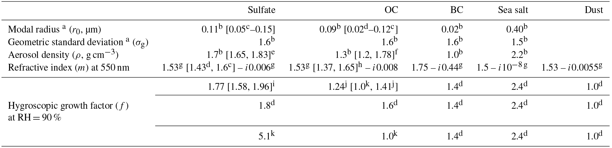
^a Assuming lognormal distributions for all aerosol species except for dust. The effective radius is calculated as $r_{\mathrm{e}}=r_{\mathrm{0}}{e}^{\left(\frac{\mathrm{5}}{\mathrm{2}}{\ln }^{\mathrm{2}}{\mathit{\sigma }}_{\mathrm{g}}\right)}$. ^b Drury et al. (2010). ^c Highwood et al. (2009). ^d Chin et al. (2002). ^e Sarangi et al. (2016). ^f Park et al. (2006). ^g OPAC (Hess et al., 1998). ^h Moise et al. (2015). ⁱ κ parameter (Petters and Kreidenweis, 2007). The hygroscopic factor (f) is calculated as f(RH) $={\left(\mathrm{1}=\mathit{\kappa }\frac{\mathrm{RH}}{\mathrm{100}-\mathrm{RH}}\right)}^{\mathrm{1}/\mathrm{3}}$ following Snider et al. (2016), where κ=0.53 in the default run, κ=0.33 for the low end, and κ=0.72 for the high end. ^j Calculated from the κ parameter equation, where κ=0.1 in the default run, and κ=0.2 for the high end (Jimenez et al., 2009; Duplissy et al., 2011). ^k Empirical hygroscopic growth factors used by the revised IMPROVE algorithm (Hand and Malm, 2006) to calculate light extinction (http://vista.cira.colostate.edu/Improve/the-improve-algorithm/, last access: 9 January 2019). The revised IMPROVE algorithm assumes no hygroscopic growth for OC.

Download Print Version | Download XLSX

2.4 Ground-based observations

The AErosol RObotic NETwork (AERONET) is a federated instrument network that provides ground-based information about aerosols including AOD, derived from sun photometer measurements of direct solar radiation (Holben et al., 1998). We use Level-2 (cloud screened and quality assured) daily average data from 13 sites over the northeastern US. We also include observed AOD from the Distributed Regional Aerosol Gridded Observation Networks (DRAGON)-USA 2011 field campaign, co-located with the DISCOVER-AQ aircraft campaign. The DRAGON campaign provides extensive sun photometer measurements of AOD at 38 sites along the flight path of DISCOVER-AQ from 1 July to 15 August 2011, which were incorporated into the AERONET database. To allow direct comparison with AOD_MAIAC and AOD_CMAQ, AERONET AOD measurements at 0.44 and 0.675 µm were interpolated to 0.55 µm using the Ångström exponent (the first derivative of AOD with wavelength, on a logarithmic scale) provided.

We use ground-based measurements of daily 24 h average PM_2.5 from 152 EPA Air Quality System (AQS) sites over the northeastern US. Of the 152 sites, 13 sites have AERONET sites within 10 km of them (about the resolution of CMAQ). We consider these 13 sites to be “co-located” and use them to evaluate uncertainties in modeled PM_2.5∕AOD relationships. We also use AQS aerosol speciation data at 54 sites, which include the Chemical Speciation Network (CSN) and the Interagency Monitoring of Protected Visual Environments (IMPROVE) visibility monitoring network.

To evaluate the modeled vertical profile of ambient RH, we use ground-based soundings from six radiosonde sites over the northeastern US. Aggregated daily data at 00:00 and 12:00 UTC are acquired from the NOAA Integrated Global Radiosonde Archive (IGRA), and modeled vertical profiles are sampled concurrently with radiosonde observations. We use the RH data calculated from vapor pressure, saturation vapor pressure, and ambient air pressure (Durre and Yin, 2008).

2.5 NASA DISCOVER-AQ 2011 field campaign

The NASA DISCOVER-AQ (Deriving Information on Surface conditions from Column and Vertically Resolved Observations Relevant for Air Quality) aircraft campaign over Baltimore–Washington, D.C. in July 2011 provides extensive, systematic, concurrent measurements of aerosol chemical, optical, and microphysical properties. The NASA P-3B aircraft performed 14 flights, which include 247 profiles (typically extending from 0.4 to 3.2 km above the surface) over six DRAGON sites (Crumeyrolle et al., 2014). We use the simultaneous measurements of aerosol composition (SNA, OC, BC), scattering, absorption, and extinction coefficients in dry (RH < 40 %), ambient, and wet (RH > 80 %) environments. To reduce the random uncertainties of individual observations and to allow direct comparison with CMAQ and ground-based observations, we aggregate the daily aircraft profiles horizontally to six locations corresponding to the six sites, and vertically to CMAQ model layers, and then we sample CMAQ modeled values consistently with observations.

3.1 Deriving surface PM_2.5 from satellite observations

We derive satellite-based PM_2.5 (hereafter PM_{2.5_MAIAC}) over the northeastern US for 2011 by taking the product of daily average CMAQ modeled PM_2.5∕AOD relationships (PM_{2.5_CMAQ}∕AOD_CMAQ) with MAIAC AOD (AOD_MAIAC, Eq. 1). These unconstrained PM_2.5 estimates (Fig. 1) are independent of surface observations. As PM_{2.5_MAIAC} is determined as the product of observed AOD_MAIAC and modeled PM_{2.5_CMAQ}∕AOD_CMAQ, the spatial patterns of PM_{2.5_MAIAC} will be affected by the spatial variations in both AOD_MAIAC and PM_{2.5_CMAQ}∕AOD_CMAQ. Figure 1a shows the summertime average (June, July, and August, JJA) AOD_MAIAC at 1 km resolution overlaid with AERONET observed AOD. While we find high AOD over some populated urban areas such as New York City (NYC), high AOD_MAIAC is also found over central New York State (NYS), away from major anthropogenic sources. In CMAQ, PM_2.5 (PM_{2.5_CMAQ}) occurs over regions with major anthropogenic sources such as NYC. AOD_CMAQ also shows a latitudinal dependence, with higher AOD at lower latitudes, which reflects (1) relatively high emissions of aerosol and its precursors from anthropogenic and biogenic sources over Maryland, Pennsylvania, and NYC and (2) latitudinal variations in RH that affect aerosol hygroscopic growth. The modeled PM_{2.5_CMAQ}∕AOD_CMAQ varies spatially (1 standard deviation (SD) is 45 µg m⁻³ per unit of AOD), mainly driven by the spatial variations in PM_{2.5_CMAQ} (R=0.86). We find the overall spatial pattern of satellite-derived PM_2.5 correlates more strongly with modeled PM_{2.5_CMAQ}∕AOD_CMAQ (R=0.97) than observed AOD_MAIAC (R=0.8), suggesting that the large-scale spatial variability reflects modeled rather than satellite-based distributions, at least under our framework for the northeastern US in summer. The temporal variability in PM_{2.5_MAIAC} is also mainly driven by variability in PM_{2.5_CMAQ}∕AOD_CMAQ (R=0.61), with little temporal correlation between regional average AOD_MAIAC and PM_{2.5_MAIAC} (R=0.05, Fig. 2). At short timescales, the daily variability in regional average PM_{2.5_MAIAC} shows stronger correlation with PM_{2.5_CMAQ}∕AOD_CMAQ in all seasons except for JJA, when PM_{2.5_MAIAC} values are driven by variability in both AOD_MAIAC (R=0.5) and PM_{2.5_CMAQ}∕AOD_CMAQ (R=0.4, Fig. 2). Summertime AOD_MAIAC is higher than wintertime AOD by 50 %, while summertime PM_{2.5_MAIAC} is lower than in winter by 46 %. Previous studies also found inconsistent seasonal cycles in AOD and PM_2.5 (Ford et al., 2013; Kim et al., 2015). We attribute the opposite seasonal cycle in PM_{2.5_MAIAC} and AOD_MAIAC to three factors: (1) weak boundary layer ventilation in winter that leads to sharp vertical gradients of aerosol distribution (Kim et al., 2015), (2) higher RH in summer that leads to larger hygroscopic growth, and (3) model overestimates of PM_2.5 (especially OC) in wintertime and underestimates of PM_2.5 in summertime, leading to an overestimate of the winter-to-summer decrease in PM_{2.5_CMAQ}∕AOD_CMAQ (see Sect. 3.3).

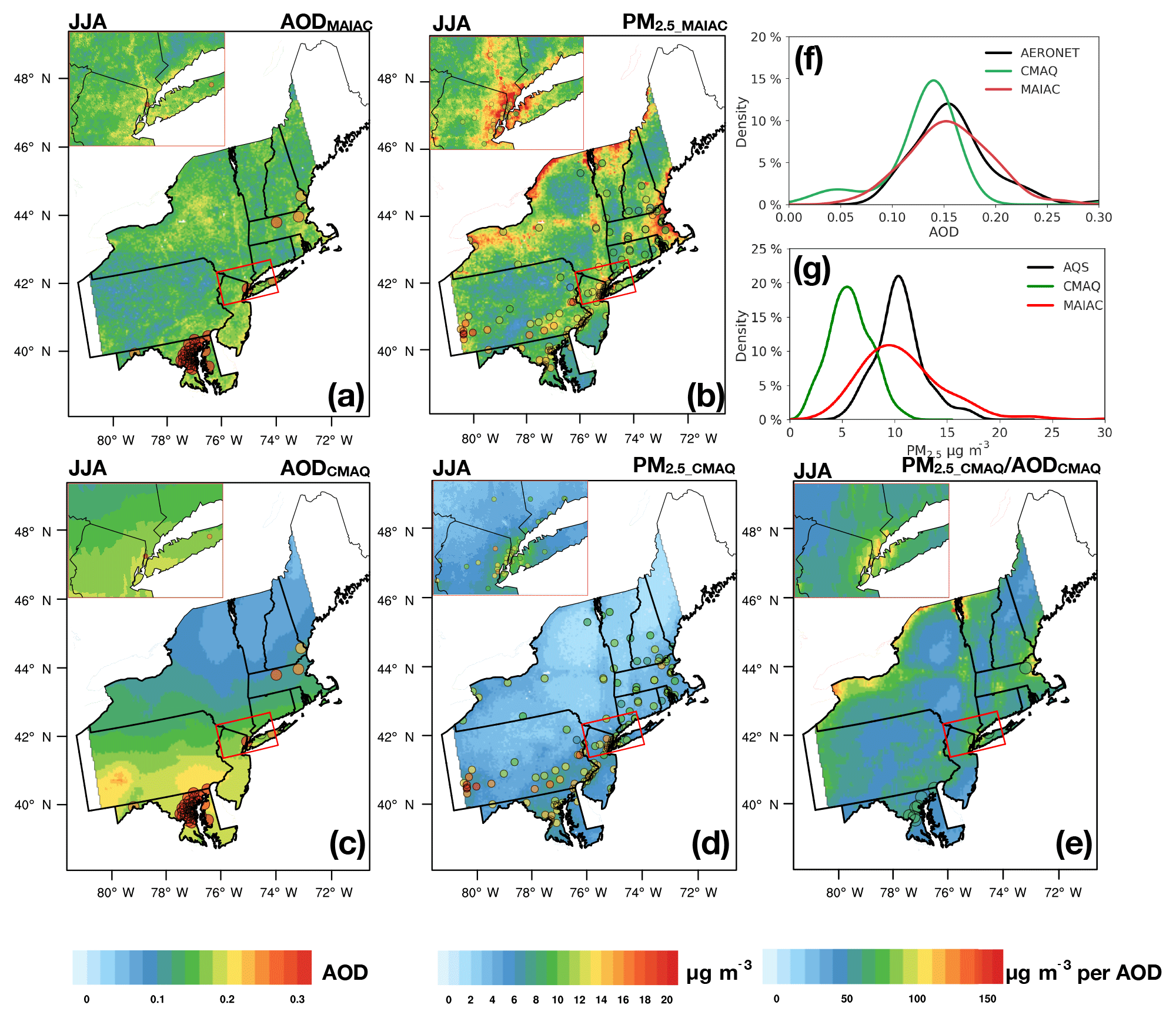
Figure 1Summertime (JJA) average (a) MAIAC AOD (AOD_MAIAC), (b) satellite-derived PM_2.5 (PM_{2.5_MAIAC}), (c) CMAQ model AOD (AOD_CMAQ), (d) CMAQ model PM_2.5 (PM_{2.5_CMAQ}), and (e) CMAQ modeled PM_2.5∕AOD (PM_{2.5_CMAQ}∕AOD_CMAQ) ratio overlaid with ground-based observations (AERONET, AQS, co-located AERONET and AQS sites) over the northeastern US with zoom-in maps over the New York City region in the upper left corner. (f) Density plot of AOD showing the distribution of MAIAC, CMAQ, and AERONET observed AOD sampled at AERONET sites. (g) Density plot of PM_2.5 showing the distribution of satellite-derived, CMAQ, and AQS observed PM_2.5 sampled at AQS sites.

Download

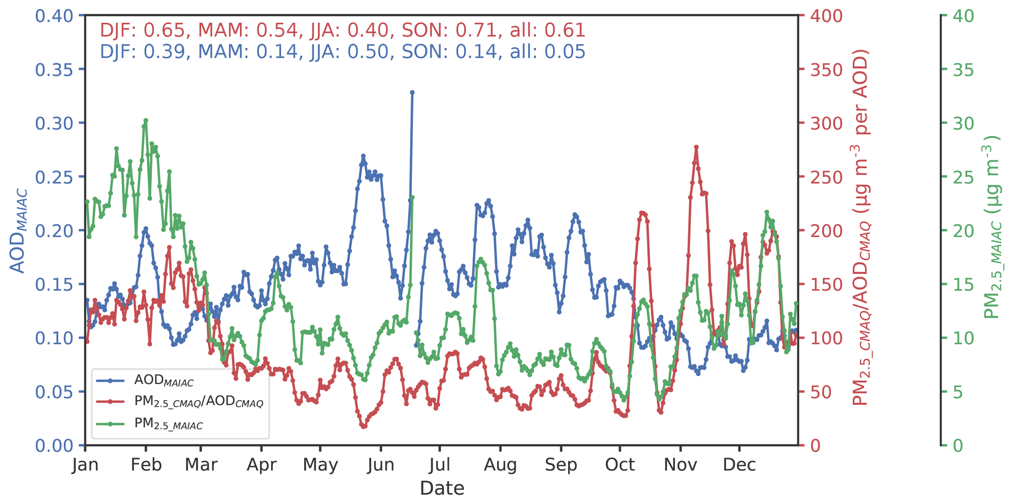
Figure 2Regional 10-day running average of (a) MAIAC AOD (AOD_MAIAC, blue), (b) CMAQ modeled PM_2.5∕AOD relationship (PM_{2.5_CMAQ}∕AOD_CMAQ, red), and (c) satellite-derived PM_2.5 (PM_{2.5_MAIAC}, green). The numbers on the upper left corner show the Pearson correlation coefficients (R) of PM_{2.5_MAIAC} with PM_{2.5_CMAQ}∕AOD_CMAQ (red) and AOD_MAIAC (blue).

Download

While at larger spatial scales PM_{2.5_CMAQ}∕AOD_CMAQ contributes more to the spatial and temporal variability in PM_{2.5_MAIAC} than AOD_MAIAC, at smaller scales, over which we assume the spatial variability in PM_2.5∕AOD is homogenous, incorporating fine-resolution satellite data reveals stronger spatial gradients (e.g., enhancements along industrial corridors) than PM_{2.5_CMAQ} (Fig. 1b). In addition to refining spatial resolution, satellite-derived PM_2.5 can correct model summertime biases in PM_2.5. Observed AOD from AERONET and PM_2.5 from AQS indicate an overall underestimate in both AOD_CMAQ (Fig. 1c; normalized mean bias (NMB) = −44 %) and PM_{2.5_CMAQ} (Fig. 1d; NMB = −17 %) in summer. We find PM_{2.5_CMAQ}∕AOD_CMAQ is overall consistent with the observed PM_2.5∕AOD sampled at co-located AQS–AERONET sites (NMB = 0.9 %) as the ratio largely cancels out the model underestimates in both PM_2.5 and AOD. AOD distributions retrieved from MODIS (AOD_MAIAC) agree better with AERONET AOD than AOD_CMAQ (NMB = 5 %, Fig. 1f), though we find small low biases at two sites in NYC and at most DRAGON sites over Maryland. Our derived distribution of PM_{2.5_MAIAC} is thus closer to PM_2.5 observed at AQS sites than PM_{2.5_CMAQ} (NMB = 4.7 % vs. 44 % for PM_{2.5_CMAQ}, Fig. 1g). However, the PM_{2.5_MAIAC} distribution is wider than observed at AQS: the lowest 5 % is 5 vs. 7 µg m⁻³ for PM_{2.5_MAIAC} vs. AQS PM_2.5, and the highest 5 % is 16 vs. 13 µg m⁻³. We find that PM_{2.5_MAIAC} is biased high over NYC, coastal regions of Massachusetts, the borders of upstate New York, and northern Vermont. Evaluation of PM_{2.5_MAIAC} in other seasons shows larger biases and uncertainties (Fig. S1 in the Supplement). In the following sections, we examine sources of uncertainties and biases in satellite-derived PM_2.5. We quantify the uncertainties in terms of bias (systematic) and random uncertainty. The bias uncertainty is linked to the overall accuracy, while the random uncertainty reflects random fluctuations in the measurements or the imprecision of the model resulting from imperfect modeling assumptions and simplifications.

3.2 Evaluation of satellite-observed AOD products

AOD_MAIAC in general agrees well with AERONET observations (spatial R=0.83, temporal R=0.85, MB  = −0.01, and RMSE = 0.07). The performance of AOD_MAIAC evaluated at northeastern US AERONET sites is consistent with the evaluation of Superczynski et al. (2017) over North America (R=0.82, MB = −0.008). We find, however, that AOD_MAIAC in winter (December, January, and February, DJF) is biased high by 49 % ($\mathrm{MB}=+\mathrm{0.02}$) on average. The wintertime overestimate is likely due to residual snow contamination, which is below the detection limit, even though we applied a stringent data quality filter to remove pixels flagged as snow. We find the wintertime overestimate is most evident over northern latitudes (e.g., AERONET sites in Massachusetts; NMB ranges from 80 % to 180 %), where snow occurs more often. The NMBs of AOD_MAIAC are 15 % in March, April, and May (MAM), −5 % in JJA, and 17 % in September, October, and November (SON), though the quantile range of the error is large, suggesting that single observations have large random uncertainties (Fig. 3). Taking the 1σ standard deviation of the normalized biases as a metric of random uncertainty, we estimate the uncertainties of daily satellite observations to be around 80 % in DJF, 60 % in MAM and SON, and 50 % in JJA. Spatial and/or temporal averaging can reduce these random errors of satellite observations, which is evidenced as the smaller spread of errors than for monthly averages at the same spatial resolution, or daily data at coarser (10 km) resolution, but it does not reduce the overall MB between AOD_MAIAC and AOD_AERONET (Fig. 3). We find that spatially averaging AOD_MAIAC to 10 km leads to an overall increase in AOD_MAIAC. Temporal averaging, however, leads to an overall decrease in AOD_MAIAC except for DJF, leading to a smaller positive MB in SON (7 %) and MAM (7 %), but larger negative MB in JJA (−8 %) and positive MB (67 %) in DJF.

Figure 3Distribution of normalized biases of AOD_MAIAC evaluated at 52 AERONET (including DRAGON, only available for JJA) sites in four seasons of 2011 over the northeastern US using daily MAIAC AOD at 1 km resolution and 10 km resolution and monthly average MAIAC AOD composite (only including days when both satellite and AERONET measurements are available) at 1 km resolution. The box shows the interquartile range (IQR) while the whiskers extend to show the rest of the distribution with outliers (points that are either 1.5× IQR or more above the third quantile or below the first quantile) removed. The red triangles show the seasonal mean normalized biases. Note that the normalized bias is an asymmetric metric, for which model overestimates are unbounded, whereas model underestimates are bounded by −100 %; therefore the mean of normalized biases is typically higher than the median of the normalized biases.

Download

3.3 Evaluation of modeled PM_2.5∕AOD relationships

Three factors contribute to the overall uncertainty in the modeled PM_2.5∕AOD relationship: (1) PM_{2.5_CMAQ}, (2) AOD_CMAQ, and (3) the relation between (1) and (2). We evaluate uncertainties of the three factors at 13 paired AQS–AERONET sites (within 10 km of each other; about the resolution of CMAQ). Figure 4 shows the distribution of the biases of modeled daily PM_{2.5_CMAQ}, AOD_CMAQ, and PM_{2.5_CMAQ}∕AOD_CMAQ compared with observations. Generally, PM_{2.5_CMAQ} biases vary seasonally: from +42 % in DJF to −39 % in JJA on average. In contrast, AOD_CMAQ biases show weaker seasonality. The NMBs of AOD_CMAQ are 3 % in DJF, −16 % in MAM, −7 % in JJA, and −20 % in SON. On the daily scale, biases of AOD_CMAQ are weakly correlated with the biases of PM_{2.5_CMAQ} (R=0.14), suggesting model biases in AOD do not necessarily reflect biases in modeled PM_2.5. This is in contrast with prior analysis of annual means for which emission biases drive similar biases in AOD and PM_2.5 (van Donkelaar et al., 2013). The better accuracy of emissions in the northeastern US than elsewhere in the world allows processes other than emissions to be more important for the northeastern US. We find the seasonal biases in modeled PM_2.5 are retained in the PM_{2.5_CMAQ}∕AOD_CMAQ ratio, which exceeds the biases of PM_{2.5_CMAQ} in DJF, MAM, and SON. As both PM_{2.5_CMAQ} and AOD_CMAQ are biased low in JJA, the modeled PM_2.5∕AOD bias (−20 %) is smaller than that of PM_{2.5_CMAQ} (−39 %). Biases in PM_{2.5_CMAQ} and AOD_CMAQ are oppositely signed in fall, leading to the largest mean biases of modeled PM_2.5∕AOD (+74 %). The spread of the biases of PM_{2.5_CMAQ}∕AOD_CMAQ is larger than that of PM_{2.5_CMAQ} and AOD_CMAQ, with the standard deviation ranging from 50 % in JJA to 100 % in SON.

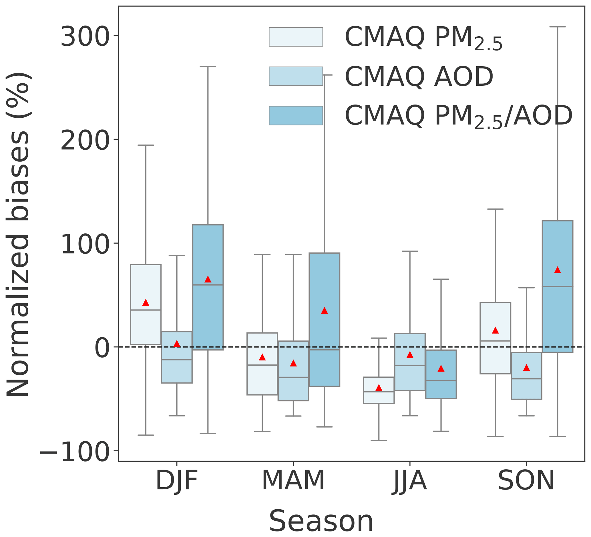
Figure 4As in Fig. 3 but for daily PM_{2.5_CMAQ}, AOD_CMAQ, and PM_{2.5_CMAQ}∕AOD_CMAQ in each season of 2011 evaluated at 11 co-located AQS–AERONET sites over the northeastern US.

Download

3.4 Relative importance of satellite AOD versus modeled PM_2.5∕AOD to uncertainties in satellite-derived PM_2.5

We have shown that both satellite AOD and modeled PM_2.5∕AOD are subject to large uncertainties at the daily timescale. To directly compare the relative importance of the biases of satellite AOD vs. model PM_2.5∕AOD for the satellite-derived PM_2.5, we scale the biases of modeled PM_2.5∕AOD with daily AOD_MAIAC, so that the biases are expressed in units of PM_2.5 (µg m⁻³):

We then scale the biases of AOD_MAIAC with the daily modeled PM_2.5∕AOD relationship:

We can also interpret ΔPM_{2.5_AOD} and ΔPM_{2.5_Rel} as the changes in derived PM_2.5 if we use “true” observed AOD or PM_2.5∕AOD instead of AOD_MAIAC or modeled PM_2.5∕AOD. As shown in Fig. 5a, mean biases caused by modeled PM_2.5∕AOD are +9.2 µg m⁻³ in DJF, +2.8 µg m⁻³ in MAM, −3.3 µg m⁻³ in JJA, and +7.7 µg m⁻³ in SON, which introduces larger biases to the derived PM_2.5 than the MAIAC satellite product in all seasons (7.6 µg m⁻³ in DJF, +1.3 µg m⁻³ in MAM, −0.7 µg m⁻³ in JJA, and 0.9 µg m⁻³ in SON). Using the root-mean-squared ΔPM_{2.5_AOD} to quantify the random uncertainty, satellite AOD contributes an overall random error of 8.3 µg m⁻³ to daily satellite PM_{2.5_MAIAC} with the smallest error in JJA (5.1 µg m⁻³) and largest error in DJF (13.2 µg m⁻³), while modeled PM_2.5∕AOD contributes an error of 10.8 µg m⁻³ (root-mean-squared ΔPM_{2.5_Rel}), with the smallest error in JJA (6.5 µg m⁻³) and largest error in SON (15.2 µg m⁻³). The spread of the biases is larger for modeled PM_2.5∕AOD than that for MAIAC AOD except for DJF. Our findings are consistent with Ford and Heald (2016), who use a higher-resolution (nested) version of the GEOS-Chem model and MODIS Dark Target AOD (Collection 6) to estimate 2 times larger uncertainties in surface PM_2.5 resulting from modeled PM_2.5∕AOD relationships than in satellite AOD.

Figure 5(a) Box plots comparing the distribution of biases in daily PM_{2.5_MAIAC} due to observational uncertainties in AOD_MAIAC (green, ΔPM_{2.5_AOD}) versus model uncertainties in PM_{2.5_CMAQ}∕AOD_CMAQ (blue, ΔPM_{2.5_Rel}), evaluated consistently at 11 co-located AQS–AERONET sites over the northeastern US. (b) Pearson correlation coefficient between the biases in daily satellite-derived PM_2.5 (ΔPM_{2.5_MAIAC}, evaluated with AQS observations) and the biases in PM_{2.5_AOD} attributed to observational uncertainties in AOD_MAIAC (ΔPM_{2.5_AOD}) versus model uncertainties in PM_{2.5_CMAQ}∕AOD_CMAQ (ΔPM_{2.5_Rel}). ΔPM_{2.5_AOD} is calculated by multiplying the biases of AOD_MAIAC with daily modeled PM_2.5∕AOD relationships (Eq. 8). ΔPM_{2.5_Rel} is calculated by multiplying the modeled PM_2.5∕AOD biases with daily AOD_MAIAC (Eq. 9). The red triangles show the seasonal mean biases.

Download

At the daily timescale, both ΔPM_{2.5_AOD} and ΔPM_{2.5_Rel} show large day-to-day variability: the 1σ standard deviation is 10.5 µg m⁻³ for daily ΔPM_{2.5_AOD} and 8.3 µg m⁻³ for daily ΔPM_{2.5_Rel}. Next, we evaluate the dependence of the biases of satellite-derived PM_2.5 (denoted as ΔPM_{2.5_MAIAC}; evaluated with AQS observed PM_2.5) on ΔPM_{2.5_Rel} versus ΔPM_{2.5_AOD} by evaluating the Pearson correlation coefficients (R). Overall, ΔPM_{2.5_MAIAC} is more strongly correlated with ΔPM_{2.5_Rel} (R=0.85) than with ΔPM_{2.5_AOD} (R=0.53), indicating the uncertainties of modeled PM_2.5∕AOD are a more important driving factor to the uncertainties of daily satellite-derived PM_2.5, which could explain 72 % variance (R²) in ΔPM_{2.5_MAIAC}. In JJA, however, ΔPM_{2.5_MAIAC} is moderately correlated with both ΔPM_{2.5_AOD} (R=0.48) and ΔPM_{2.5_Rel} (R=0.49), suggesting uncertainties of modeled PM_2.5∕AOD and satellite AOD contribute equally to the uncertainties of satellite-derived PM_2.5. We note that there is no statistically significant correlation between ΔPM_{2.5_Rel} and ΔPM_{2.5_AOD}, with R ranging from −0.4 in SON to 0.23 in JJA, which suggests that the errors caused by modeled PM_2.5∕AOD and by satellite AOD are independent of each other.

3.5 Factors leading to uncertainties in modeled PM_2.5∕AOD relationship

Uncertainties in the modeled PM_2.5∕AOD relationship mainly reflect uncertain aerosol speciation, aerosol vertical profiles, ambient RH, and parameterizations for aerosol optical properties including aerosol density, size distribution, refractive index, and hygroscopic growth. Here we quantify the uncertainties from each factor and evaluate their impacts on the derived PM_2.5.

3.5.1 Aerosol speciation

Aerosol optical properties vary with chemical composition. Model biases in the aerosol composition also affect the overall representation of particle hygroscopicity. For the same PM_2.5 abundance, variations in the aerosol composition may alter the particle optical properties, especially hygroscopicity, and consequently the PM_2.5∕AOD relationship. Figure 6a compares the modeled aerosol composition with ground-based observations averaged for each season. High biases in PM_{2.5_CMAQ} in winter are largely due to model overestimates of OC by a factor of 3, and low biases in summer are due to a combination of underestimated SNA and OC. As a result, CMAQ overestimates the fraction of OC by about 20 % in DJF, 15 % in MAM, and less than 10 % in other seasons, while it underestimates the fraction of SNA by 5 % to 20 % in all seasons.

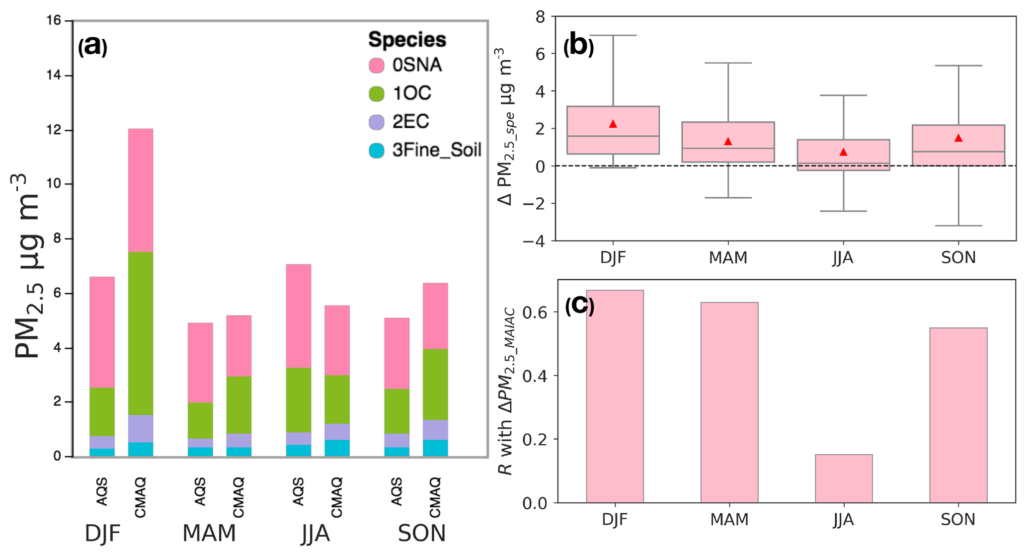
Figure 6(a) Seasonal average PM_2.5 speciation from CMAQ vs. AQS observations in 2011 evaluated at 54 CSN and IMPROVE sites. (b) Box plots showing the distribution of estimated biases of daily satellite-derived PM_2.5 due to model biases in PM_2.5 speciation (ΔPM_{2.5_spe}) by season for 2011. Red triangles show the seasonal mean biases. (c) Pearson correlation coefficient between the biases in PM_{2.5_MAIAC} (ΔPM_{2.5_MAIAC}) and ΔPM_{2.5_spe}.

Download

To estimate the impacts of model biases in aerosol speciation on AOD_CMAQ and PM_{2.5_MAIAC}, we keep the total aerosol mass the same and redistribute AOD (AOD_{CMAQ_ir}) of each species i based on the observed fraction of each species (i.e., SNA, OC, elemental carbon (EC), soil dust; sea salt was excluded due to the limited ground-based measurements and its negligible contribution):

$$\begin{array}{}\text{(10)}& {\mathrm{AOD}}_{\mathrm{CMAQ}\mathrm{\_}\mathrm{ir}}={\displaystyle \frac{{\mathrm{PM}}_{i\mathit{\_}\mathrm{obs}}}{{\mathrm{PM}}_{\mathrm{TOT}\mathrm{\_}\mathrm{obs}}}}\times {\displaystyle \frac{{\mathrm{PM}}_{\mathrm{TOT}\mathit{\_}\mathrm{CMAQ}}}{{\mathrm{PM}}_{i\mathit{\_}\mathrm{CMAQ}}}}\times {\mathrm{AOD}}_{\mathrm{CMAQ}\mathit{\_}i},\end{array}$$

where PM_{TOT_obs} and PM_{TOT_CMAQ} are the total aerosol mass from observations and CMAQ, respectively, which are reconstructed by summing up SNA, OC, EC, and soil dust. Next, we estimate the uncertainty due to speciation as the differences in derived PM_{2.5_MAIAC} (ΔPM_{2.5_spe}) using the redistributed AOD_{CMAQ_ir} instead of the original AOD_CMAQ, shown in Fig. 6b. As SNA generally has the largest mass extinction efficiency (MEE), a low bias in SNA leads to an overall underestimate of AOD_CMAQ and therefore an overestimate of PM_{2.5_MAIAC}, which is largest in winter (MB = 2.2 µg m⁻³, SD = 2.6 µg m⁻³) and smallest in summer (MB = 0.7 µg m⁻³, SD = 3.0 µg m⁻³). The estimated biases due to speciation show seasonal cycles similar to those of the modeled PM_2.5∕AOD biases (Fig. 4), suggesting that aerosol speciation errors contribute to the seasonality in modeled PM_2.5∕AOD biases. Overall, model–observation discrepancy in speciation causes an error (root-mean-squared ΔPM_{2.5_spe}) of 4.0 µg m⁻³. On a daily basis, the correlation (R) between ΔPM_{2.5_spe} and ΔPM_{2.5_MAIAC} is over 0.5 for all seasons except JJA, which means model biases in speciation alone can explain more than 25 % variance (R²) in ΔPM_{2.5_MAIAC}. Biases in speciation in JJA have relatively smaller impacts on the derived PM_2.5, which contribute less than 1 µg m⁻³ MB and show weak correlation with ΔPM_{2.5_MAIAC} (R=0.15).

3.5.2 Aerosol vertical profile

A caveat on the results in the Sect. 3.5.1 is that we assume the model errors in speciation are constant across all vertical layers, as AQS sites only provide observations near the surface. The DISCOVER-AQ aircraft campaign measured vertical variations in aerosol composition, although spatial and temporal coverage is limited. Figure 7a compares the modeled and observed vertical distributions of SNA, OC, and BC averaged over the DISCOVER-AQ campaign. We do not discuss sea salt and dust here since they contribute a negligible portion of the total aerosol mass in this region. Both the model and observations show SNA contributes more than half of the total aerosol across all vertical layers (Fig. 7). Aircraft observations show SNA decreases gradually with altitude with a nearly constant vertical gradient, while SNA_CMAQ is well mixed below 1.5 km and starts to decline at the same rate as SNA_aircraft above 1.5 km (Fig. 7). CMAQ underestimates SNA below 1.5 km but overestimates SNA at higher altitudes. The positive model bias of SNA at higher altitudes may be due to excessive vertical transport or overestimation of RH (Sect. 3.4.3) and consequently overestimation of SO₂ oxidation rate and aerosol water uptake. OC, however, is biased low at all altitudes, which is likely due to inaccurate treatment of the production of secondary organic aerosol (SOA) (Zhang et al., 2009). The newer version of CMAQv5.1 shows higher SOA concentration in summer with the introduction of new SOA species (Appel et al., 2017). BC is generally low during the campaign (typically lower than 0.3 µg m⁻³). BC_CMAQ generally agrees well with BC_aircraft, though BC_CMAQ tends to overestimate BC between 1 and 3 km. Figure 7b compares CMAQ modeled and observed total aerosol mass (SNA + OC + BC) averaged during the campaign. CMAQ modeled aerosol mass is on average biased low below 2 km and biased high at higher altitudes (Fig. 7b).

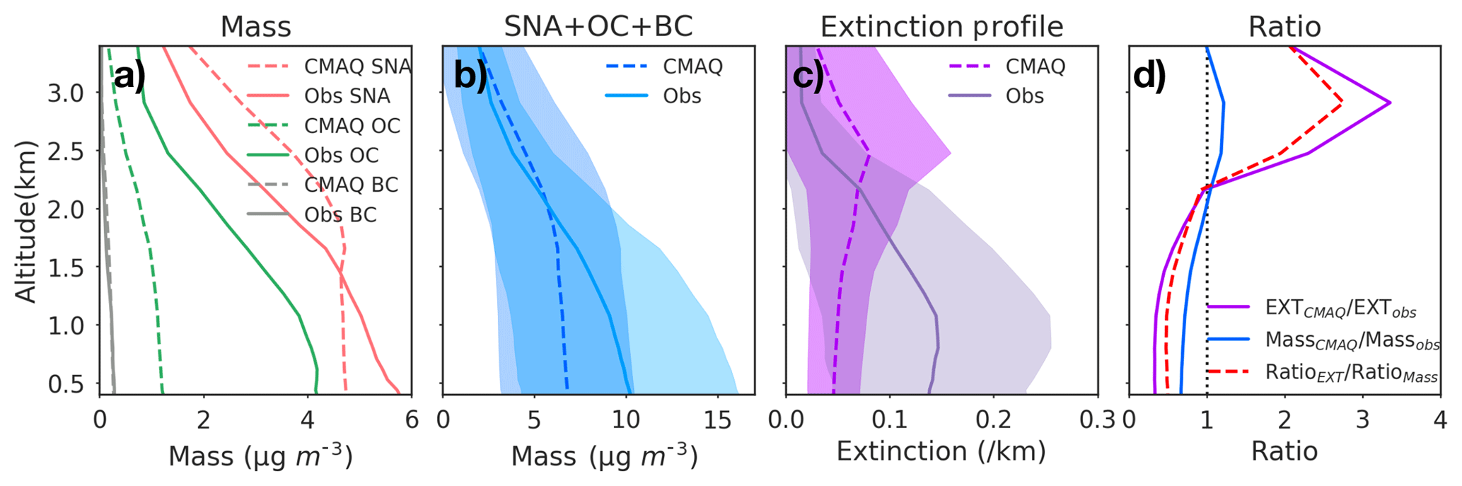
Figure 7Campaign-mean vertical profiles of (a) aerosol composition, (b) total mass (SNA + OC + BC), and (c) extinction from CMAQ vs. observations from the DISCOVER-AQ 2011 Baltimore–Washington, D.C. campaign. (d) Campaign-mean vertical profile of the model-to-observation ratio of extinction (Ratio_EXT), total aerosol mass (Ratio_Mass), and Ratio_EXT∕Ratio_Mass. Aircraft observations are first aggregated to match model layers, and corresponding model values are sampled concurrently with the time of observations. CMAQ modeled extinction is estimated with FlexAOD using the default parameters in Table 1. The shading in (b) and (c) shows the standard deviation of the day-to-day variability.

Download

Next, we evaluate how the vertical distribution of aerosols relates to extinction. Figure 7c compares the modeled and observed average vertical extinction profiles. We find, consistent with the biases in mass, a low bias in the modeled extinction profile below 2 km and a high bias above (Fig. 7c). The biases in extinction and the biases in mass have the same signs for more than 80 % of data pairs and are strongly correlated (R=0.85). This suggests that the aerosol vertical profile of extinction is mainly indicative of mass distribution. However, column AOD measures the vertical integral of light extinction by aerosols, which means the modeled AOD biases would be proportional to modeled surface PM_2.5 biases only if the biases in extinction are constant across all vertical layers. Since the biases of extinction change sign at higher altitude, the AOD biases reflect the competing effects of negative biases near the surface and positive biases at high altitudes, which lead to an overall negative bias of the PM_2.5∕AOD relationship, consistent with the negative NMB of PM_2.5∕AOD in July shown in Fig. 4.

To explore the causes of the model–observation discrepancy in extinction and the resulting impacts on the satellite-derived surface PM_2.5, we calculate the vertical extinction profile in CMAQ by replacing the modeled aerosol mass distribution (SNA, OC, BC), total MEE (ratio of total mass to extinction), or RH with those of the aircraft observations, as shown in Fig. 8a. Replacing the modeled aerosol mass with observations, we find a decrease in extinction at high altitudes (above 2.5 km) and increase at low altitudes (below 2.5 km), but replacing the aerosol mass alone does not explain all of the model–observation differences. At high altitudes, only replacing the modeled total MEE without changing the mass captures the observed extinction. We attribute the model overestimate of extinction to model overestimation of extinction efficiency at high altitudes. A major contributor to the model overestimate of total MEE is its excessive RH at high altitudes, which leads to an overestimate of the hygroscopic growth. Replacing RH with observations largely corrects the high biases aloft but does not correct the low biases below 2 km (Fig. 8a). At lower altitudes, the model low biases are due to model underestimates of both aerosol mass and total MEE. Model underestimates of MEE are likely due to (1) uncertain optical properties, (2) other aerosols or gases (e.g., NO₂, O₃), or liquid clouds that can scatter or absorb light.

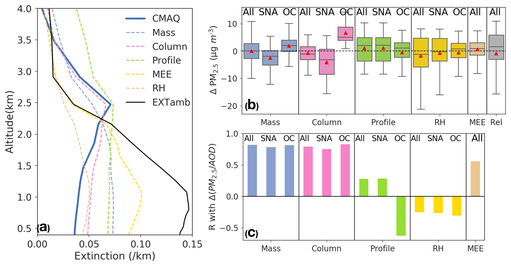
Figure 8(a) Campaign-mean vertical profiles of extinction calculated from CMAQ speciated aerosol fields using FlexAOD and those calculated by replacing modeled speciated aerosol mass (Mass), total column mass (Column), vertical profile shape (Profile), total mass extinction efficiency (MEE), and relative humidity (RH) with those observed during the DISCOVER-AQ 2011 Baltimore–Washington, D.C. campaign. EXT_amb is the aircraft observed vertical extinction profile. (b) Box plots of the distribution of biases of PM_{2.5_MAIAC} attributed to each factor shown in (a), and the biases of PM_{2.5_MAIAC} attributed to modeled PM_2.5∕AOD (Rel). Red triangles show the mean biases. (c) Pearson correlation coefficient between the biases in modeled PM_2.5∕AOD relationships and the biases in modeled PM_2.5∕AOD attributed to individual factors shown in (b).

Download

Figure 8b shows the biases of PM_{2.5_MAIAC} due to model uncertainties in vertical profiles of aerosol mass or MEE or RH, estimated by calculating the changes in PM_2.5 when we replace the model vertical profiles with observations. Since the aircraft altitude ranges from 0.3 to 3.4 km, we use modeled values for the layers below 0.3 and above 3.4 km while attempting to minimize the discontinuity at both boundaries through vertical interpolation. As SNA and OC contribute most to extinction, we also evaluate the biases of vertical profiles of SNA and OC separately. We find that replacing modeled aerosol mass with observed mass leads to small positive biases in PM_{2.5_MAIAC} (MB = 0.05 µg m⁻³, SD = 4.3 µg m⁻³), due to the combined effects of negative biases from SNA (MB = −2.5 µg m⁻³, SD = 4.7 µg m⁻³) and positive biases from OC (MB = +1.9 µg m⁻³, SD = 4.3 µg m⁻³).

We further separate the model–observation discrepancy in the vertical profiles as differences in total column mass versus in vertical profile shape by (1) keeping the modeled vertical distribution but adjusting the mass of each species uniformly so that the total column mass is equal to observation and (2) keeping the total column mass the same as in the model but redistributing the aerosol based on the observed vertical profiles. We find that redistributing the aerosol vertical profile leads to a positive mean bias in PM_{2.5_MAIAC} (MB = 1.1 µg m⁻³, SD = 4.9 µg m⁻³), while the model–observation discrepancy in column mass leads to a negative mean bias (MB = −0.6 µg m⁻³, SD = 3.6 µg m⁻³) (Fig. 8b). The positive biases in the profile shape are mainly attributed to model biases of the vertical profile of SNA (MB = 1.2 µg m⁻³, SD = 5.0 µg m⁻³), which shows a larger fraction of SNA at higher altitude where aerosol is less effective at scattering light due to lower RH. The negative MB of column mass reflects a combination of negative biases of SNA (MB = −4.1 µg m⁻³, SD = 5.6 µg m⁻³) due to model overestimates of SNA column mass and positive bias of OC (MB = 6.7 µg m⁻³, SD = 4.4 µg m⁻³) due to model underestimates of column mass of OC. Model biases in MEE lead to a small positive MB of 0.6 µg m⁻³.

Using the observed PM_2.5∕AOD acquired from paired AQS–AERONET sites, we estimate that model biases in modeled PM_2.5∕AOD lead to a negative MB of −0.9 µg m⁻³ with large day-to-day variability (SD = 9.8 µg m⁻³) during the DISCOVER-AQ campaign, reflecting the model biases from different sources as discussed above. Next, we evaluate which factor drives the daily variability in the modeled PM_2.5∕AOD biases the most by evaluating the R value between the estimated biases in modeled PM_2.5∕AOD versus that attributed to individual factors. We find model bias in aerosol mass is the most deterministic factor for the biases in modeled PM_2.5∕AOD (R=0.82, Fig. 8c). Model biases in aerosol mass can be due to either biases in column mass or vertical profile shape. We find model biases in modeled PM_2.5∕AOD are more dependent on the biases in aerosol column mass (R=0.79), instead of vertical profile shape. Model biases in MEE show moderate correlation with model biases of PM_2.5∕AOD (R=0.56). While model uncertainties in RH lead to an overall negative bias (MB = −1.7 µg m⁻³, SD = 7.4 µg m⁻³) to PM_{2.5_MAIAC}, they are negatively correlated with model biases of PM_2.5∕AOD ($R=-\mathrm{0.25}$).

3.5.3 RH

Figure 8 suggests model biases in RH contribute a negative bias to the derived PM_{2.5_MAIAC} during the DISCOVER-AQ aircraft campaign. Here we evaluate the impacts of modeled RH (RH_CMAQ) biases on derived PM_2.5 throughout the year using six atmospheric soundings over the northeastern US. We only assess the impacts of RH on the optical properties (i.e., hygroscopic growth) of aerosols. Comparing RH_CMAQ with observed RH (RH_obs), RH_CMAQ is overall biased high with the largest biases in winter. To evaluate the resulting impacts on AOD_CMAQ, we recalculate the extinction using observed ambient RH from the soundings instead of RH_CMAQ in Eq. (4). Replacing RH_CMAQ with RH_obs decreases extinction by ∼50 % on average from the surface to 5 km in both JJA and DJF (black lines in Fig. 9a and b). As AOD is the vertical integral of extinction, the total area between EXT_sonde and EXT_CMAQ (gray shading in Fig. 9a and b) indicates the differences in AOD due to differences in RH. The differences in RH below 3 km in DJF, MAM, and SON contribute more than 80 % to the total differences in AOD. In JJA, the contribution from higher versus lower altitudes is similar, despite small model RH biases below 2 km.

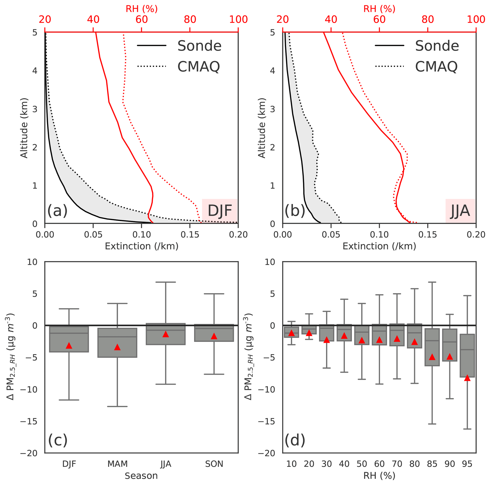
Figure 9(a) DJF and (b) JJA average vertical profiles of the CMAQ modeled versus observed RH at six atmospheric soundings over the northeastern US, and the modeled extinction versus that calculated by replacing modeled RH with observed values. The gray area shows the difference in the two extinction profiles, with the total area being the difference in AOD. (c) Box plots showing the impacts of model bias of RH on the derived PM_{2.5_MAIAC} (ΔPM_{2.5_RH}) in four seasons of 2011, which are calculated by comparing the PM_{2.5_MAIAC} minus the one calculated using observed RH. (d) Box plots show the influence of model RH biases on the derived PM_{2.5_MAIAC} (ΔPM_{2.5_RH}) as a function of observed near-surface RH.

Download

We evaluate how the model–observation discrepancy in RH affects the derived PM_2.5 by calculating the changes in PM_{2.5_MAIAC} (ΔPM_{2.5_RH}) if EXT_sonde is used instead of EXT_CMAQ. As expected, model errors in RH lead to a negative bias in derived PM_{2.5_MAIAC} of 3 µg m⁻³ on average (Fig. 9c). The negative biases in PM_{2.5_MAIAC} due to RH are largest in spring (−3.5 µg m⁻³) and smallest in summer (−1.6 µg m⁻³). The hygroscopic growth factor is nonlinearly correlated with RH, which increases more rapidly at high RH (> 80 %) than at low to median RH (< 80 %, Fig. S2). Compared with median RH conditions, model RH errors lead to more than double ΔPM_{2.5_RH} (−6.4 µg m⁻³ vs. 3 µg m⁻³) when observed near-surface RH > 80 % (Fig. 9d). At RH > 95 %, we find that the ΔPM_{2.5_RH} can be as large as −20 µg m⁻³ (Fig. 9d). Despite the large impacts of model errors of RH at humid conditions, there is no significant correlation between ΔPM_{2.5_RH} and ΔPM_{2.5_MAIAC} (R=0.18, evaluated at nearby sites within 10 km), suggesting that uncertainty in RH is not a main contributor to the random uncertainties in satellite-derived PM_2.5.

3.5.4 Uncertainties in the parameterization of aerosol optical properties

In previous sections, we demonstrated that the satellite-derived PM_2.5 depends on the accuracy of the model simulation. Even with a perfect simulation, satellite-derived PM_2.5 will be sensitive to the parameterization of aerosol optical properties, which would affect the MEE. We evaluate the uncertainties associated with the parameterization of aerosol optical properties by varying each parameter (Table 1), and we calculate the corresponding changes in the derived PM_{2.5_MAIAC}. Figure 10 shows the range of uncertainty in annual average PM_{2.5_MAIAC} due to uncertain aerosol size distributions, hygroscopicity, refractive index, and aerosol species density.

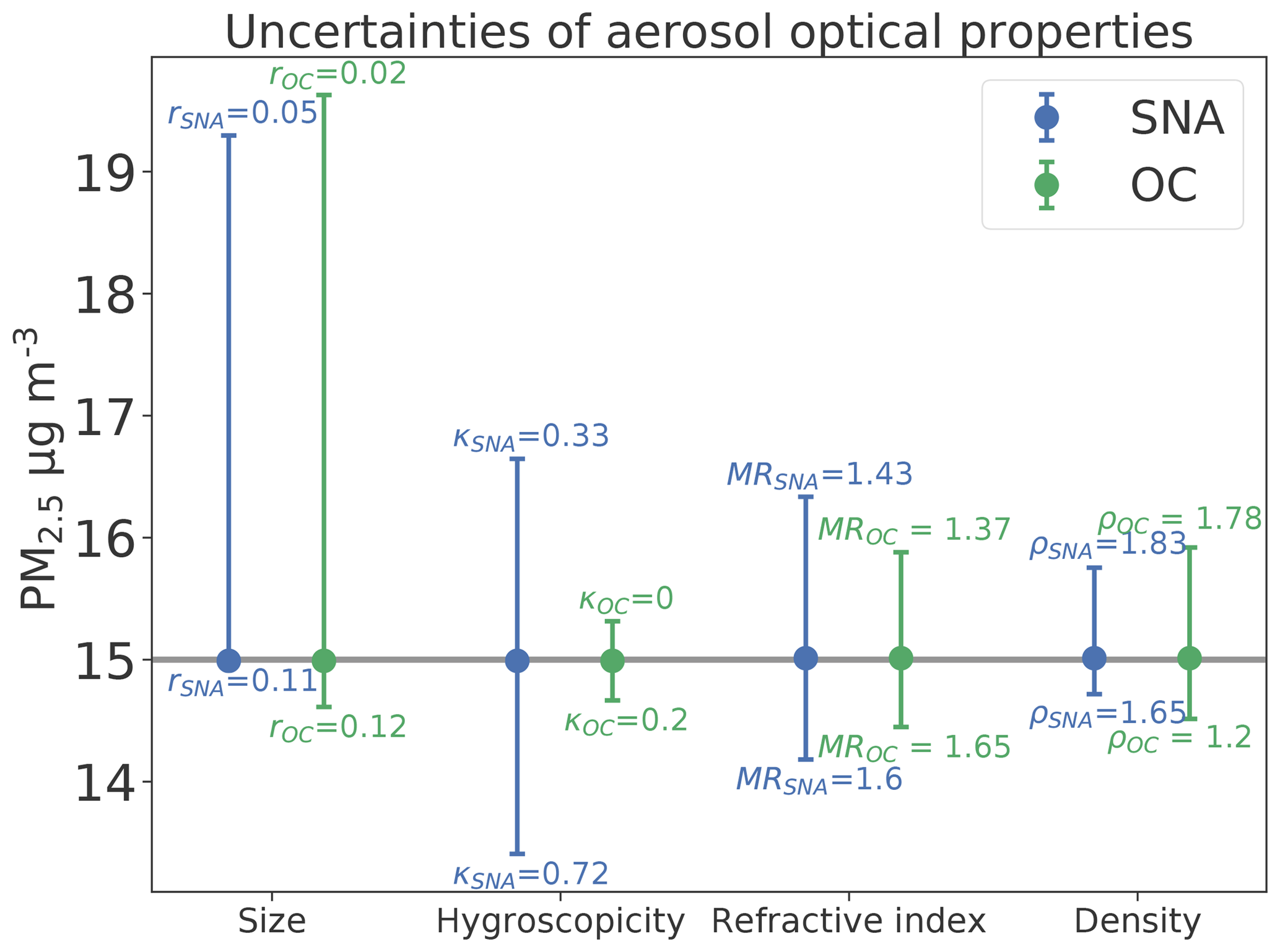
Figure 10Uncertainties in annual average satellite-derived PM_{2.5_MAIAC} due to uncertainties of size distribution, hygroscopicity, refractive index, and aerosol species density of sulfate–nitrate–ammonium (SNA; blue) and organic carbon (OC; green) sampled over AQS sites. The circle shows the annual average satellite-derived PM_{2.5_MAIAC} using the default parameters to calculate AOD_CMAQ in FlexAOD (Table 1). The error bars represent the range of PM_{2.5_MAIAC} using different values for each parameter. The labels indicate the corresponding minimum or maximum parameter values that produce the range shown in PM_{2.5_MAIAC}. The horizontal line at 15 µg m⁻³ indicates the annual average PM_{2.5_MAIAC} calculated using default values for each aerosol optical property in the base FlexAOD.

Download

The size of a particle is a defining characteristic of aerosol light extinction (Mishchenko et al., 1999). To evaluate model sensitivities to the uncertainties in size distribution, we vary the r₀ of SNA from 0.05 to 0.15 with a 0.02 increase each time to cover the range of values reported in the literature. For OC, we calculate AOD_CMAQ with r₀=0.02, 0.06, 0.09, and 0.12 µm, all values used in previous studies (Hess et al., 1998; Chin et al., 2002; Highwood, 2009; Drury et al., 2010). Annual average PM_{2.5_MAIAC} could vary by up to 5 µg m⁻³ (32 %) with the choice of a modal radius of either r_SNA or r_OC, which is the largest source of uncertainty among the four parameters (Fig. 10). We find that AOD_CMAQ reaches a maximum with r_SNA=0.07 µm (r_eff=0.12 µm) and minimum with r_SNA=0.05 (r_eff=0.15 µm), while PM_{2.5_MAIAC} reaches a maximum with r_SNA=0.05 (r_eff=0.09 µm) and minimum with r_SNA=0.11 (r_eff=0.19 µm), suggesting the impacts of size distribution are nonlinear and nonuniform (Fig. S3). Mie scattering of a particle tends to be most effective when the particle's diameter is near the wavelength of interest (0.55 µm). As hygroscopic particle growth also affects the size distribution, depending on ambient RH and the hygroscopic growth factor, reducing (or increasing) the dry effective radius could move the bulk aerosol size either closer to or further from 0.55 µm and thus either increase or decrease the extinction. For OC, as the effective radius and the hygroscopic growth factor are smaller than for SNA, increasing the modal radius leads to more effective scattering, and thus larger AOD_CMAQ and smaller PM_{2.5_MAIAC}. Relative to the default r_OC=0.09 µm assumed by Drury et al. (2010), using the r_OC (0.02 µm) recommended by Chin et al. (2002a) increases PM_{2.5_MAIAC} by 5 µg m⁻³ (32 %) on average, worsening the positive biases of PM_{2.5_MAIAC}. Increasing r_OC to 0.12 µm as recommended by Highwood et al. (2009) has little effect, decreasing PM_{2.5_MAIAC} by 2 % on average.

The uncertainty of hygroscopicity lies in two aspects: (1) the function shape and (2) the parameters. Figure S2 compares the κ function shape with the hygroscopic growth factors used by the IMPROVE network (Hand and Malm, 2006), the default algorithm used to calculate AOD online in CMAQ, with that proposed by Chin et al. (2002) (Table 1). Using the DISCOVER-AQ aircraft data to evaluate the parameterization of hygroscopic growth, we find that the κ parameter best characterizes the observed hygroscopic growth factor (Fig. S2c). Latimer and Martin (2018) similarly found that implementing a κ formulation instead of hygroscopic growth based on OPAC improved the GEOS-Chem representation of mass scattering efficiency. Thus, we choose the κ parameter to represent the hygroscopic growth factor, and the uncertainty estimate here only reflects uncertainties in the κ parameter. In practice, changes in aerosol composition could have even larger effects on hygroscopicity than uncertainties in κ as discussed in Sect. 3.5.1.

To test the sensitivity of satellite-derived PM_2.5 to uncertainties in the κ parameter, we compute AOD_CMAQ using the low (0.33) and high end of κ (0.72) for SNA as suggested by Koehler et al. (2006). As the hygroscopic properties of inorganic salts are relatively well known, the range of uncertainty for f(RH) of SNA is 30 % at most (Fig. S2b). OC, however, is composed of thousands of species with distinct hygroscopicities. Assuming κ_OC ranges from 0 (non-hygroscopic) to 0.2 (Jimenez et al., 2009; Duplissy et al., 2011), the range of f(RH) of OC can be as large as a factor of 2 at high RH > 96 % (Fig. S2a). Despite the larger uncertainty of κ_OC, we find the overall impacts of the uncertainties of κ_OC on the derived PM_2.5 (0.3 µg m⁻³, 2 % of annual average PM_{2.5_MAIAC}) are smaller than those of κ_SNA (1.6 µg m⁻³, 11 % of annual average PM_{2.5_MAIAC}). The small impacts of κ_OC reflect the relatively small portion and the less hygroscopic nature of OC. For single observations, varying κ_SNA leads to a maximum increase in PM_{2.5_MAIAC} by 20 % and a maximum decrease by 28 %. Varying κ_OC increases PM_{2.5_MAIAC} by 10 % or decreases PM_{2.5_MAIAC} by 18 % at most. The overall impact of the uncertainties of κ_SNA ranks second among the four parameters for SNA, while κ_OC has the smallest impacts on the derived PM_2.5 (Fig. 10).

The refractive index (m) determines the Mie extinction efficiency, which is subject to uncertainties mostly due to the lack of measurements (Kanakidou et al., 2005). m_SNA in OPAC (default value) is slightly different from that recommended in Chin et al. (2002) and Highwood (2009). Moise et al. (2015) suggest m_OC varies by species, with its real part ranging from 1.37 to 1.65. We calculated another version of AOD_CMAQ by varying the real part of m_SNA and m_OC using the lowest and highest values reported in the literature. We find the annual average PM_{2.5_MAIAC} decreased by 0.8 µg m⁻³ (6 %) using the high end of m_{R_SNA}, while it increased by 1.3 µg m⁻³ (9 %) on average using the low end. Though m_{R_OC} has a wider range of uncertainty, its impacts on PM_{2.5_MAIAC} (−4 % to +6 %) are smaller than that of m_{R_SNA}. While the overall impacts on PM_{2.5_MAIAC} due to uncertainties of m_{R_SNA} are generally within 10 % for single observations, PM_{2.5_MAIAC} can change by more than 20 % under SNA-dominated and high-RH environments. The overall uncertainty due to m_{R_OC} is generally within 5 % for single observations, with a few cases (< 10 % of the total data) in which the relative change in PM_{2.5_MAIAC} can exceed 10 %.

As aerosol density (ρ) is assumed to be constant for each species, varying ρ has the same effect on the extinction of given species. We vary the aerosol density of SNA from 1.65 to 1.83 g cm⁻³ based on the uncertainty estimate from a laboratory study of Sarangi et al. (2016), which translates to an uncertainty of −3 % to 7 % for AOD_SNA, and the aerosol density of OC from 1.2 to 1.78 g cm⁻³ following Park et al. (2006), which translates to an uncertainty in AOD_OC ranging from −8 % to 37 %. We find aerosol species density, in general, contributes least to the overall uncertainty in satellite-derived PM_2.5. Varying ρ_OC across the range in Table 1 increases annual average PM_{2.5_MAIAC} by 0.9 µg m⁻³ (6 %) or decreases it by 0.6 µg m⁻³ (3 %) at most. As the aerosol density of inorganic salt is less uncertain, varying ρ_sulf leads to negligible changes in annual average PM_{2.5_MAIAC} at both the high (0.7 µg m⁻³, 5 %) and low (−0.5 µg m⁻³, −2 %) ends.