the Creative Commons Attribution 4.0 License.
the Creative Commons Attribution 4.0 License.
 | 04 Mar 2019
Evaluating models' response of tropical low clouds to SST forcings using CALIPSO observations
Grégory Cesana
Anthony D. Del Genio
Andrew S. Ackerman
Maxwell Kelley
Gregory Elsaesser
Ann M. Fridlind
Ye Cheng
Mao-Sung Yao
Recent studies have shown that, in response to a surface warming, the marine tropical low-cloud cover (LCC) as observed by passive-sensor satellites substantially decreases, therefore generating a smaller negative value of the top-of-the-atmosphere (TOA) cloud radiative effect (CRE). Here we study the LCC and CRE interannual changes in response to sea surface temperature (SST) forcings in the GISS model E2 climate model, a developmental version of the GISS model E3 climate model, and in 12 other climate models, as a function of their ability to represent the vertical structure of the cloud response to SST change against 10 years of CALIPSO (Cloud-Aerosol Lidar and Infrared Pathfinder Satellite Observations) observations. The more realistic models (those that satisfy the observational constraint) capture the observed interannual LCC change quite well ( % K−1 vs. % K−1) while the others largely underestimate it ( % K−1). Consequently, the more realistic models simulate more positive shortwave (SW) feedback ( W m−2 K−1) than the less realistic models ( W m−2 K−1), in better agreement with the observations ( W m−2 K−1), although slightly underestimated. The ability of the models to represent moist processes within the planetary boundary layer (PBL) and produce persistent stratocumulus (Sc) decks appears crucial to replicating the observed relationship between clouds, radiation and surface temperature. This relationship is different depending on the type of low clouds in the observations. Over stratocumulus regions, cloud-top height increases slightly with SST, accompanied by a large decrease in cloud fraction, whereas over trade cumulus (Cu) regions, cloud fraction decreases everywhere, to a smaller extent.
- Article
(3717 KB) -
Supplement
(1972 KB) - BibTeX
- EndNote


Low-level clouds are ubiquitous in the tropics. Their presence is tied to a combination of large-scale atmospheric circulation and sea surface temperatures (SSTs), which affect temperature and moisture differences between the surface and the free troposphere (e.g., Bretherton et al., 2013; Klein and Hartmann, 1993). While the underlying processes are not fully understood, recent observationally based studies confirm that low-cloud cover (LCC) and SST are negatively correlated (e.g., McCoy et al., 2017; Myers and Norris, 2015; Qu et al., 2015). Therefore, in a warming world, all else being equal, marine boundary layer clouds are expected to dissipate somewhat, which will result in more incoming solar radiation, reinforcing the surface warming through a positive feedback. However, there is no consensus in general circulation models (GCMs) on whether the low-level cloud amount will increase or decrease in future climate projections (Klein and Hall, 2015). Moreover, not all models are able to reproduce the observed loss of low-level cloud in response to increased surface temperatures in present-day climate, and the majority continue to underestimate the low-level cloud amount (e.g., Cesana and Waliser, 2016; Zhang et al., 2005). Added together, these problems limit our confidence in future climate projections.
As a result, recent efforts have been devoted to evaluating climate models against these observations (e.g., Klein and Hall, 2015; Myers and Norris, 2016; Qu et al., 2015; McCoy et al., 2017). This is based on the assumption that models must reproduce the LCC–SST relationship in the current climate as a necessary but not sufficient condition to have confidence in their ability to simulate a more realistic future climate change in regions dominated by low clouds, although there is no guarantee that current climate variability itself is indicative of longer-term climate changes (e.g., Marvel et al., 2018). Their results suggest that models that are in better agreement with observations in this way are those with a higher climate sensitivity – i.e., a greater warming of surface temperatures in the future compared to the present-day climate.
All these studies used passive-sensor measurements to study this relationship and evaluate the models, because they provide good spatial and temporal coverage along with a long record, which reduces uncertainty in the LCC–SST relationship. However, the space-borne passive instruments typically cannot resolve the vertical extent of clouds and miss some clouds that are shielded by higher clouds. In comparison, the vertical structure of cloud changes in response to surface temperature variations has received far less attention in climate models (i.e., Myers and Norris, 2015). Yet, the two-dimensional cloud amount as seen from space (i.e., LCC) may hide compensating errors in cloud amount at different levels and does not document the thickness of the cloud. Recent literature has shown the importance of knowing the vertical structure of low clouds to improve our understanding of how clouds may respond to climate change. For example, a deepening of the planetary boundary layer (PBL) – characterized by an increase in the cloud-top heights in the low levels – allows more dry air from the free troposphere to be mixed into the PBL, subsequently reducing the cloud amount and therefore generating a positive cloud feedback (Sherwood et al., 2014). It is also hypothesized that the shallowness of the low-cloud layer in the present-day climate may be used as an emergent constraint on GCMs (Brient et al., 2016). Lastly, in addition to other information (e.g., horizontal extent), ascertaining the vertical structure of low clouds could also help in discriminating the cumulus clouds from the stratocumulus (Sc) clouds, with the former typically having higher cloud top and variability (e.g., Nuijens et al., 2015). These examples emphasize the need for further evaluation of the vertical structure of clouds in the present day and how it will evolve in a warmer climate. Thus, active remote sensing instruments can potentially provide important information about the dominant low-cloud regimes and their responses to perturbations.
In addition to providing detailed information on the vertical structure of clouds, the horizontal resolution of the Cloud-Aerosol Lidar and Infrared Pathfinder Satellite Observations (CALIPSO, Winker et al., 2010) lidar has a finer horizontal resolution than that of space-borne passive instruments (70 m footprint at the surface vs. a few hundred meters to kilometers), allowing a better detection of fractional cover of cumulus, which are radiatively dominant in many of the subsiding regions of the tropics. However, the narrow swath of the lidar – a beam diameter of 70 m every 333 m along track – produces a much smaller sample of clouds than passive instruments. Thus, active and passive techniques are complementary.
Here we propose to characterize and evaluate the response of tropical low clouds and their radiative impact to SST forcings in two generations of the GISS model E GCM, with a focus on vertical structure, using 10 years of CALIPSO satellite and Clouds and the Earth's Radiant Energy System (CERES) measurements. To put this into a larger context, we also assess this relationship for a large sample of other climate models. Finally, we identify the best-performing models, based on how well they match the observed vertical structure relationship between tropical low cloud and SST, and compare the cloud cover response to SSTs of these models against the others.
2.1 Observations
We use the GCM-Oriented CALIPSO Cloud Product (CALIPSO-GOCCP) version 2.9 (Cesana et al., 2016) for the LCC and the cloud fraction from 2007 to 2016 over a 2.5∘ grid and for 40 levels with 480 m spacing from 0 to 19.2 km. CALIPSO-GOCCP (i) was developed to facilitate the evaluation of cloud properties in GCMs when combined with a lidar simulator (Chepfer et al., 2008) that uses the same cloud definitions and (ii) ensures a consistent comparison between observations and simulations. The ratio of the total attenuated backscatter signal (ATB) to the molecular ATB – so-called scattering ratio (SR) – is computed every 333 m along-track near-nadir profile for 480 m height intervals. This quantity is a proxy of the presence of particulate matter in a layer. GOCCP-CALIPSO uses a fixed SR threshold to detect clouds (SR>5), for either daytime or nighttime data, regardless of the vertical level. This threshold allows the detection of thin cirrus cloud in the high troposphere (McGill et al., 2007), i.e., the majority – if not all – of optically thicker PBL clouds except when masked by overlying high clouds in regimes of weak subsidence (e.g., the trade wind regions), and prevents most false detections of aerosol layers as being cloudy in the PBL (Chepfer et al., 2013). However, strong attenuation by liquid-topped low clouds may generate an underestimation of the cloud fraction underneath, close to the surface (0 to 960 m, e.g., Cesana et al., 2016), although it does not affect cloud cover. CALIPSO-GOCCP has been validated against in situ (Cesana et al., 2016) and ground-based observations (Lacour et al., 2017). Caveats for this dataset are discussed in Cesana et al. (2016) and in Cesana and Waliser (2016). To avoid daytime noise contamination on the lidar signal, we only use nighttime data; however the results using nighttime and daytime data are similar with a slightly larger amplitude of interannual LCC changes (∼10 % larger, % K−1 instead of −3.59 % K−1).
To derive an uncertainty estimate of the relationship between monthly cloud amount change and SST anomalies over several years, referred to as interannual change, we use four different datasets for the SST: European Centre for Medium-Range Weather Forecasts (ECMWF) Reanalysis Interim (ERA-Interim, Dee et al., 2011), Extended Reconstructed SST version 5 (ERSSTv5, Huang et al., 2017), NOAA Optimum Interpolation (OI) SST version 2 (NOAA-OI SSTv2, Reynolds et al., 2002) and Centennial in situ Observation-Based Estimates SST version 2 (COBE-SST2, Hirahara et al., 2014). The uncertainty related to clouds is due to the cloud threshold and the attenuation of the lidar beam. However, these are reproduced in the model via the use of the lidar simulator and therefore do not necessitate further investigation here. The “actual” observed relationship may be biased low because of the lidar attenuation and the sensitivity of the dataset to the cloud threshold. While lidar-only products of LCC agree with each other (e.g., Chepfer et al., 2013) some disagreements exist in their cloud profiles due to different definitions of cloudy and fully attenuated pixels in their algorithm (Cesana et al., 2016; Chepfer et al., 2013). Additionally, CloudSat–CALIPSO combined products have been shown to retrieve larger cloud fraction in regimes of weak subsidence but these datasets are only available for a short period of time (Mace and Zhang, 2014) and are therefore unsuited for this study. For radiative fluxes, we use the monthly CERES Energy Balanced and Filled (EBAF) edition 4 dataset (CERES-EBAF 4.0, Loeb et al., 2018). The large-scale circulation (ω500) is obtained from the monthly ERA-Interim reanalysis (Dee et al., 2011). All datasets are averaged over a 2.5∘ horizontal grid and are used over the same time period as CALIPSO-GOCCP. Using a finer grid (1∘) does not impact the results (not shown).
2.2 Simulations
In this study, we analyze prescribed-SST (Atmospheric Model Intercomparison Project, AMIP) monthly outputs from two generations of the GISS GCM. The first one is the GISS-E2 model that was used for the Coupled Model Intercomparison Project Phase 5 (CMIP5) (Schmidt et al., 2014). The second one is a developmental version of the GISS-E3 model that will be submitted to CMIP6 and will undergo additional changes and tunings by then. Over 2007–2015, this version has a small positive radiative imbalance (0.29 W m−2) of a few tenths of a W m−2 less than that estimated for the real world in the early 21st century (0.6 W m−2). E3 and E2 differ in many ways that can potentially affect low clouds:
-
Layering in lower troposphere. E2 uses a 40-layer vertical grid, whereas these E3 runs use 62 levels with the greatest refinement in the lower atmosphere: at the surface and at 850 hPa pressure, nominal layer thicknesses for E2 are respectively 20 and 35 hPa, and for the 62-layer grid they are 10 and 20 hPa.
-
Turbulence. The E2 scheme (Yao and Cheng, 2012), which includes nonlocal transport and does not consider moist processes, has been replaced by the scheme of Bretherton and Park (2009) for E3, which includes moist processes in the computation of turbulent fluxes and uses a novel relaxation approach to parameterize the nonlocal transport of turbulent kinetic energy (TKE) within well-mixed regions; the turbulent transfer coefficients it computes are applied to all prognostic variables separately, with a water-cloud-only saturation adjustment applied immediately after the transport is treated, using the scheme described below for stratiform cloud macrophysics. The Galperin et al. (1988) scheme that is used by the Bretherton and Park (2009) has been replaced by a second-order scheme with a larger critical Richardson number.
-
Stratiform cloud macrophysics. While designed differently, both E2 and E3 use a diagnostic determination of cloud fraction as a function of grid-mean moisture and a condition-dependent sub-grid variance expressed as a threshold grid-mean relative humidity (RH) for cloud formation. The Sundqvist-type scheme of E2 (Del Genio et al., 1996), applied identically to water and ice clouds, is replaced for E3 by a scheme that uses a triangular probability density function (PDF) to compute water cloud fraction and cloud water mixing ratio (Smith, 1990). For E3, ice cloud fraction is obtained independently via inversion of that PDF scheme (Wilson and Ballard, 1999), with a different variance than for water. For E3 water clouds, different prescribed values of threshold RH determine the width of the PDF for layers that are within and outside well-mixed regions as determined by the turbulence scheme; this distinction is loosely congruent to Ua and Ub in E2 (Schmidt et al., 2014, Sect. 2.5). In E2, suppression of stratiform cloud under conditions favoring convective cloud is primarily through restriction of the maximum possible areal extent of stratiform cloud to a fraction determined by the depth of convection. In E3 the following check is applied instead: if, above the PBL, a hypothetical saturated parcel is conditionally unstable, stratiform cloud is assumed to be meteorologically inconsistent with the stratification and not allowed to form except at 100 % grid-mean RH.
-
Stratiform cloud microphysics. The Sundqvist-type prognostic cloud water parameterization used in E2 (Del Genio et al., 1996) is replaced in E3 by a two-moment microphysics scheme with prognostic precipitation (Gettelman and Morrison, 2015). For our implementation we (i) use a fixed relative dispersion for the gamma size distribution of water droplets following Geoffroy et al. (2010) and the Meyers et al. (1992) expression for deposition mode heterogeneous ice nuclei and (ii) allow homogeneous aerosol freezing to occur (with a prescribed number concentration) when the RH with respect to ice (grid mean divided by the fractional threshold RH used to define the width of the PDF used for water cloud fraction) exceeds the threshold of Karcher and Lohmann (2002). Cloud droplet concentrations are prescribed with different values over land and ocean.
-
Moist convection. As in E2, the cumulus category realized for a given environment is a function of dynamically determined entrainment, which is stronger in E3 as described below. The default entrainment efficiency results in a relatively large rate producing shallow cumulus for typical subtropical conditions; this highly entraining plume may grow deeper under more unstable or moister free-tropospheric conditions. As in E2, a fraction of cloud-base mass flux seeds a second plume with a small entrainment rate conducive to deep convection when conditions are diagnosed to be favorable to mesoscale organization. The E3 version in this study relates the less-entraining fraction to the downdraft mass flux forming cold pools, mirroring Del Genio et al. (2015), whose cold pool parameterization also affects the determination of updraft properties at cloud base. This choice reduces the global frequency and shifts the pattern of less-entraining convection compared to E2, which related it to the large-scale vertical velocity. Reformulations of the numerics in E3, targeting layering independence, eliminated inadvertent but systematic reductions of entrainment rate occurring in E2. Other E2 to E3 convection changes directly affecting lower-tropospheric conditions include (a) rain evaporation above cloud base, a moistening countered by (b) more efficient venting of the PBL, with the restriction that (c) convection may only originate at the top of a turbulent layer as defined in item (3) above.
-
Convective cloud microphysics. particle size distributions (PSDs) and size–fall-speed relationships used in E2 (Del Genio et al., 2005) have been replaced for E3 with field-experiment-based normalized gamma PSDs and fall speeds for ice described by Elsaesser et al. (2017); for liquid, the E2 formulations have been replaced with bimodal (cloud and rain) drop size distributions (DSDs) (each DSD provided by Thompson et al., 2008, with a modified shape parameter from Shipway and Hill, 2012, for the rain DSD), while droplet fall speed formulations are now provided by Seifert (2008).
We note that the improved representation of stratocumulus in E3 relative to E2 is principally attributable to the implementation of the moist turbulence scheme, together with critical linkages to stratiform cloud macrophysics and moist convection.
Table 1List of other models used in this analysis in addition to GISS-E2 and GISS-E3. “Moist PBL” means that the model simulates moist processes in the PBL, by either the turbulence, the convection or both parameterizations. The stars mark the constrained models as explained in Sect. 4.1.
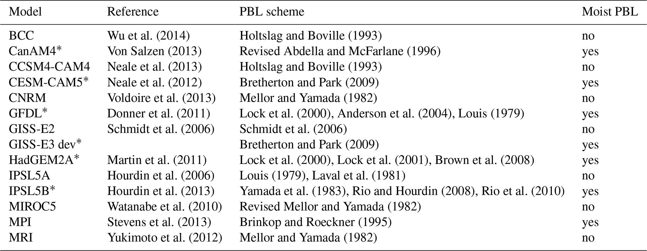
To provide context for the GISS model results, we also analyze AMIP simulations from 12 other CMIP5 models (Table 1). Except for GISS-E3 (2007–2015), we use the last 18 years of AMIP simulations (1991–2008). Using a shorter or longer time period may affect the ΔLCC∕ΔSST by a few tenths of percent per K (absolute value, Fig. S1 in the Supplement), yet it remains much smaller than the models' bias. To ensure a fair evaluation, we compare simulated and observed cloud fields through the use of the lidar simulator (e.g., Cesana and Chepfer, 2012) although the relationships found in this study are very similar (in terms of sign and shape) when original cloud fractions are utilized in GISS-E3 (see Fig. 3b). The model outputs are monthly means of the CALIPSO low-level cloud fraction (referred to as LCC in the reminder of the paper) and CALIPSO cloud fraction, so-called cllcalipso and clcalipso, respectively. The simulator package (Bodas-Salcedo et al., 2011) uses profiles of model variables (temperature, pressure, mixing ratios and cloud fraction) in each longitude–latitude grid box for each time step, divides them into sub-columns to account for sub-grid-scale variability (Klein and Jakob, 1999) and mimics the lidar simulator signal (Chepfer et al., 2008). Then, the simulated lidar signal is interpolated to the CALIPSO-GOCCP vertical resolution, 40 levels of 480 m thickness between 0 and 19.2 km, and the different diagnostics are computed and accumulated into statistics. A subpixel is diagnosed as cloudy when its SR is larger than 5 and low-level clouds are diagnosed in the column whenever a cloudy pixel is present below 3.36 km.
Although the diurnal cycle of LCC is not fully represented in the observations (sampled at 01:30 and 13:30 local time), the total-column cloud fraction mean from the lidar simulator is not substantially different from that extracted along the CALIPSO footprint (<1 % absolute difference; Cesana and Waliser, 2016) and effects on the strength of the cloud feedback have been found to be unimportant to the understanding of multimodel spread in overall cloud feedback (Webb et al., 2015).
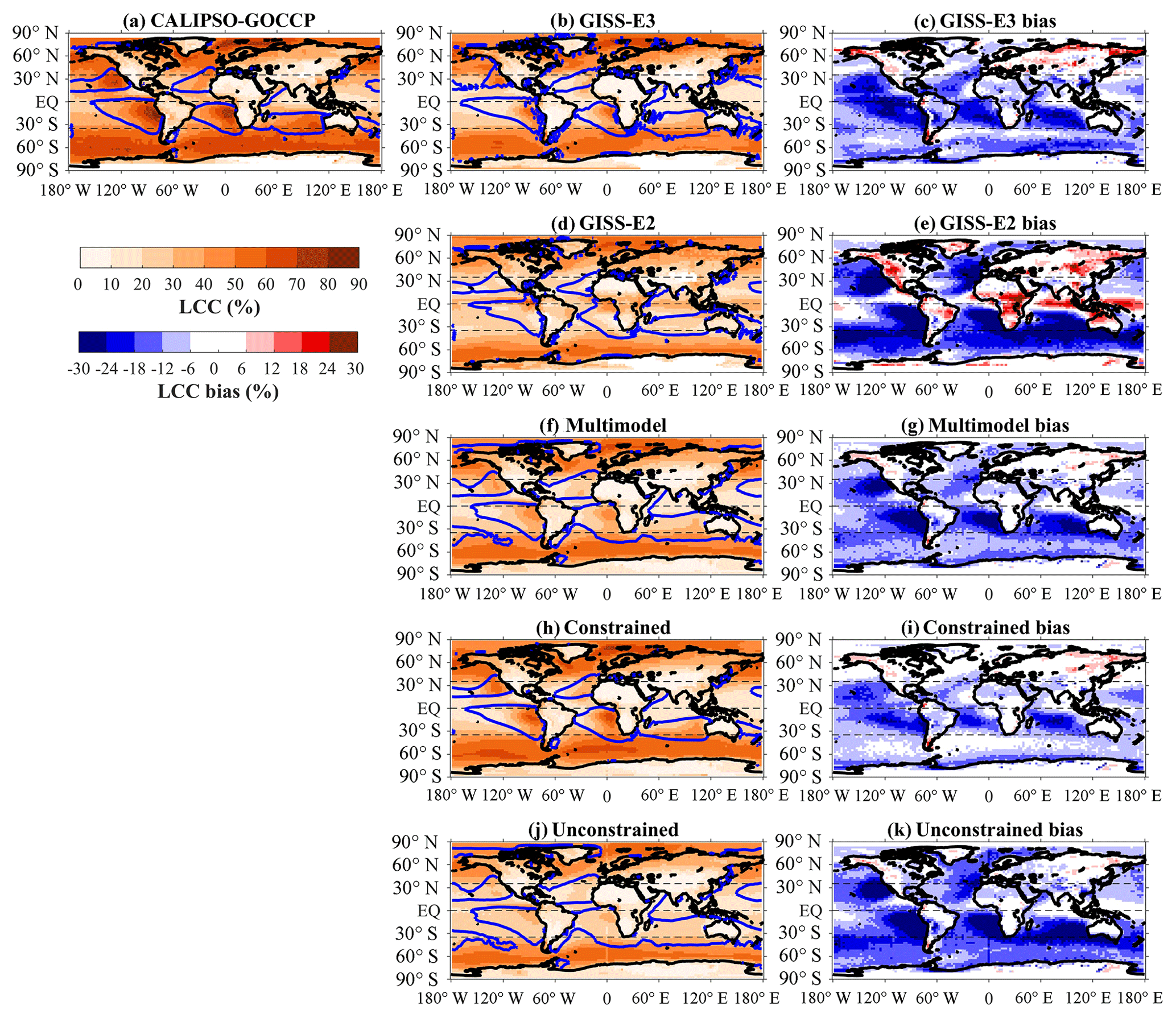
Figure 1Geographic distribution of low-cloud cover (LCC, %) for CALIPSO-GOCCP observations (a) and for GISS-E3 (b), GISS-E2 (d) and the multimodel, constrained and unconstrained models (f, h, j, respectively) along with their corresponding bias against CALIPSO-GOCCP observations (c, e, g, i ,k; models minus CALIPSO-GOCCP). The blue contour denotes the regions wherein the ω500 of each dataset (ERA-Interim reanalysis for the observations, Dee et al., 2011) is equal to 10 hPa d−1.
3.1 Definition of low-cloud regions
In this work, we focus on the low-level clouds that form over the tropical oceans (between 35∘ S and 35∘ N) in subsidence regimes defined as having a large-scale pressure vertical velocity at 500 hPa (ω500) greater than 10 hPa d−1. This filtering captures most of the stratocumulus and stratocumulus-to-shallow-cumulus transition regions, which are located climatologically within the blue contours in Fig. 1. In the literature, some studies use a 0 hPa d−1 ω500 threshold (e.g., Myers and Norris, 2015, 2016). Here we choose a more conservative ω500 threshold to minimize areas where high clouds are common and that may mask the detection of underlying low clouds in the observations. We confirm this by looking at the height at which the lidar signal becomes completely attenuated, so-called z_opaque (Guzman et al., 2017). The 10 hPa d−1 threshold almost perfectly encompasses areas where z_opaque is smaller than 2 km (see Fig. S2), meaning that the lidar is able to detect virtually all low clouds in these regions (clouds with cloud top lower than ∼3 km).
3.2 Cloud–SST relationship and observational constraint
Two main goals of our study are to investigate the interannual variation of the vertical cloud fraction (CF) and LCC in response to a change in SST in both the observations and the models and to use the observed relationship to evaluate the models. By interannual variation we mean the monthly variations over multiple years, a decade in this case. Capturing the mechanisms that govern the change in clouds in response to a surface warming is an essential condition – although not the only one – to predict future climate. Thus, we select the GCMs that produce the most realistic change in cloud profile per K of SST warming. We refer to these as “constrained models”, in the sense that they are distinguished from other models in our analysis using an observational constraint; we emphasize though that the models have not been changed in response to the observations. We compare the cloud fraction and shortwave (SW), longwave (LW) and net cloud radiative effect (CRE) changes in these models to the others, which we refer to as “unconstrained models”.
To calculate the interannual relationship between SST and cloud amount, we compute the monthly mean of CF and LCC and monthly anomalies of SST after having filtered out all grid boxes where ω500 is lower than 10 hPa d−1, referred to as CFsub, LCCsub and SSTsub, anom. Those can be seen as dynamically based means and anomalies, as opposed to spatially based anomaly and mean studies that focus on particular regions (e.g., McCoy et al., 2017; Qu et al., 2015). Hence, the cloud response is dominated by the local component rather than the large-scale component (dynamics). It is therefore complementary to imposing a uniform +4 K increase (e.g., Cesana et al., 2017) or an abrupt 4 times CO2 increase (e.g., Brient et al., 2016) that are is significantly affected by dynamical changes. We then linearly regress CFsub and LCCsub against SSTsub, anom to obtain the change (Δ) in cloud fraction and low-cloud cover per K of SST warming ΔC∕ΔSST, where C is either the CF or LCC. Using a centered finite-differencing scheme as in Myers and Norris (2015) instead of a linear regression does not impact the results (not shown).
3.3 Assumptions and caveats
By using this method, we make some assumptions that generate some caveats. For example, we assume that the relationship between SST and low-cloud amount is timescale invariant, i.e., the same regardless of the timescale over which anomalies are calculated. This assumption seems to be supported by several previous studies (e.g., Klein et al., 2017; McCoy et al., 2017), but we note that any such relevance to cloud feedback in the regions we study does not necessarily have broader implications for the global equilibrium climate sensitivity (Caldwell et al., 2018). Moreover, we analyze the effect of SST on clouds by assuming that the cloud effect on the SST is negligible on a monthly timescale based on previous studies (e.g., de Szoeke et al., 2016; Klein et al., 2017; McCoy et al., 2017). The relatively short period of the time record is another caveat here. However, the standard deviation (SD) computed using the four SST datasets (or the 5 %–95 % confidence intervals when using a single SST dataset, not shown) is far smaller than the multimodel mean SD and bias, as shown in Sect. 4. In addition, using a smaller period of time does not change the sign and shape of the results but may change its magnitude (not shown).
Other environmental factors may cause low-cloud changes such as the estimated inversion strength (EIS) or ω500 (Qu et al., 2015; Myers and Norris, 2016). When these factors are held constant the variation of the cloud amount as a function of the SST becomes a partial derivative. Past studies have shown that computing the partial derivative may decrease the magnitude of ΔLCC∕ΔSST (e.g., Myers and Norris, 2015; Qu et al., 2015). We find a similar decrease in our study using four of the five observational datasets of Sect. 4.3 ( % smaller; see Sect. 4.3).
As stated earlier, our ω500 filter targets stratocumulus and stratocumulus-to-shallow-cumulus transition regions. Such a definition of low clouds – while extensively used in the literature – does not permit us to distinguish between the two most common low-cloud types, that is to say trade cumulus (Cu) and stratocumulus, and it also excludes parts of the trade cumulus regimes that have been argued to be important to overall cloud feedback (weak convective regimes, e.g., Nuijens et al., 2015). As a consequence, our results do not target a specific type of cloud but rather represent the regional-only averaged effect of all types of low clouds. Nevertheless, we attempt to provide some information on the observed interannual changes in low clouds in trade cumulus and stratocumulus regimes in Sect. 4.3.

Figure 2Vertical profiles of cloud fraction (a, c; CF in %) and interannual cloud fraction change due to SST variations (b, d; ΔCF∕ΔSST in % K−1) as observed by CALIPSO-GOCCP observations (orange line with circles) and as simulated by the 14 models. The green line in panels (a, b) and the blue and purple lines with triangles in panels (c, d) correspond to the multimodel mean of all the models, the constrained and the unconstrained models, respectively. The dotted line denotes the height (3.36 km) used to define the low-cloud cover in CALIPSO-GOCCP.
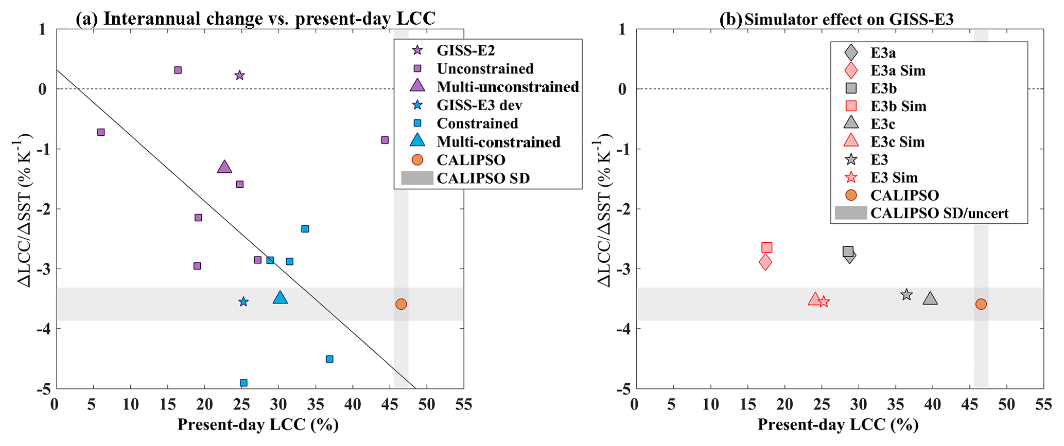
Figure 3(a) LCC change per K of SST warming (ΔLCC∕ΔSST, % K−1, y axis) as a function of the present-day LCC (%, x axis) for the models and the CALIPSO-GOCCP observations (orange circle). The unconstrained and constrained models are represented in purple and blue squares, respectively, while the stars denote the two GISS model versions, GISS-E2 in the unconstrained category and GISS-E3 development in the constrained category. The triangles correspond to the multimodel mean of each category. The solid black line is the linear regression between LCC and ΔLCC for all models but the outlier. (b) Same as (a) for four versions of GISS-E3 run along the GISS-E3 development with (black symbols) and without the simulator (red symbols). Note that while the present-day LCC is largely affected by the use of the simulator, the ΔLCC∕ΔSST is not.
4.1 Constraining the vertical response of low-level cloud fraction
Figure 2a shows averaged cloud fraction profiles over the tropical oceans (35∘ S to 35∘ N) in subsidence regimes (ω500>10 hPa d−1). In the low levels (z<3.36 km), both GISS models underestimate the CF. Although GISS-E2's peak (purple line with stars) is slightly larger than E3's (blue line with stars), the shape of the GISS-E3 profile is in better agreement with the observations (two large values at 1.2 and 1.68 km). In addition, GISS-E3's CF values are in very good agreement with the observations at 2.16 km and above while they are overestimated in GISS-E2, suggesting an excess of trade cumulus type of clouds. Most of the other models (9 out of 12) also underestimate the CF, yielding a multimodel mean peak ∼43 % smaller than observed (triangle green line, 11.2 %, vs. circled orange line, 19.6 %, Fig. 2a). In addition, the model behavior is relatively diverse, which highlights the large uncertainty around the simulation of low clouds. The observed shape of the cloud fraction profile – a single peak around 1.2 km – is not captured by all models. Some simulate a double-peak shape, which is likely the result of the distinct contribution of stratocumulus and trade cumulus clouds, with the latter having typically smaller CF and higher cloud top (typically treated by separate parameterizations in a model). Other models show a single peak as in the observations but with a far smaller CF. This could be explained by several reasons: a too-shallow PBL, a general lack of low clouds for a given thermodynamic state, a strong masking effect by overlying high clouds or by a larger influence of a convection parameterization over that of the large-scale cloud, and turbulence parameterizations that determine stratocumulus clouds.
In Fig. 2b, we show the interannual change in CF per K of SST warming (ΔCF∕ΔSST) based on a linear regression method between SST anomalies and CF, as described in Sect. 3.2. As for the mean cloud profiles, the model responses are quite diverse, generating a very large variability compared to the observed SD, while the multimodel mean captures the observed shape of ΔCF∕ΔSST to some extent. A group of models predict a very small change, which can be either an increase, a decrease or both at different heights. Others models simulate a large increase in CF at cloud top and a large decrease below, i.e., an upward shift rather than a cloud cover change. Finally, the remaining models reproduce the shape of observed change pretty well, that is to say a large decrease below 2 km.
In this study, we assume that (i) the physical mechanisms that control the subtropical low-cloud response to warmer surface temperature remain identical across all timescales and (ii) those mechanisms are essential to predict the correct subtropical low-cloud change in the future, although they may not necessarily be the only ones. For example, current climate variability does not include the radiative effect of increased CO2 on cloud-top turbulence, which may generate a reduction of stratocumulus cloud amount by increasing downwelling LW flux and thus reducing cloud-top radiative cooling (e.g., Bretherton et al., 2015). Additional phenomena, e.g., large-scale dynamical feedbacks that differ on interannual and centennial timescales, could also mitigate or amplify the change. However, we believe that the present-day interannual change in the cloud fraction (ΔCF∕ΔSST) is one important test that a model must pass to have confidence in its prediction of future climate. We therefore isolate the change in the low-cloud cover associated with a surface warming as well as the related top-of-the-atmosphere (TOA) radiative impact for the subset of models that best reproduce the observed cloud fraction change – i.e., a large CF decrease (<−1 % K−1) and no significant CF cloud-top increase (<+0.5 % K−1) (see Fig. S3 for details). In the remainder of the paper, we will call this category the constrained models (6 out of 14, marked with a star in Table 1), represented in blue, with the other models, the unconstrained models (8 out of 14), represented in purple. The two GISS models fall into each category: the unconstrained category for GISS-E2 and the constrained category for the newest version, GISS-E3.
Overall, the constrained models simulate a larger cloud amount at low levels, in better agreement with CALIPSO, than the unconstrained models (Fig. 2c). In addition to underestimating the low-level cloud amount and its decrease with surface warming, some unconstrained models predict low-level cloud top rising, either because of a deepening of the PBL or due to an increase in the upper cloud fraction peak (Fig. 2d). This cloud-top rising may imply an excess of trade cumuli in the present-day climate in the models having a dual-peak cloud fraction in the low levels (e.g., CCSM4-CAM4, MIROC, MRI, GISS-E2 and MPI; Fig. S3): one large peak close to the surface (stratocumulus type) and another smaller peak above (trade cumulus type).
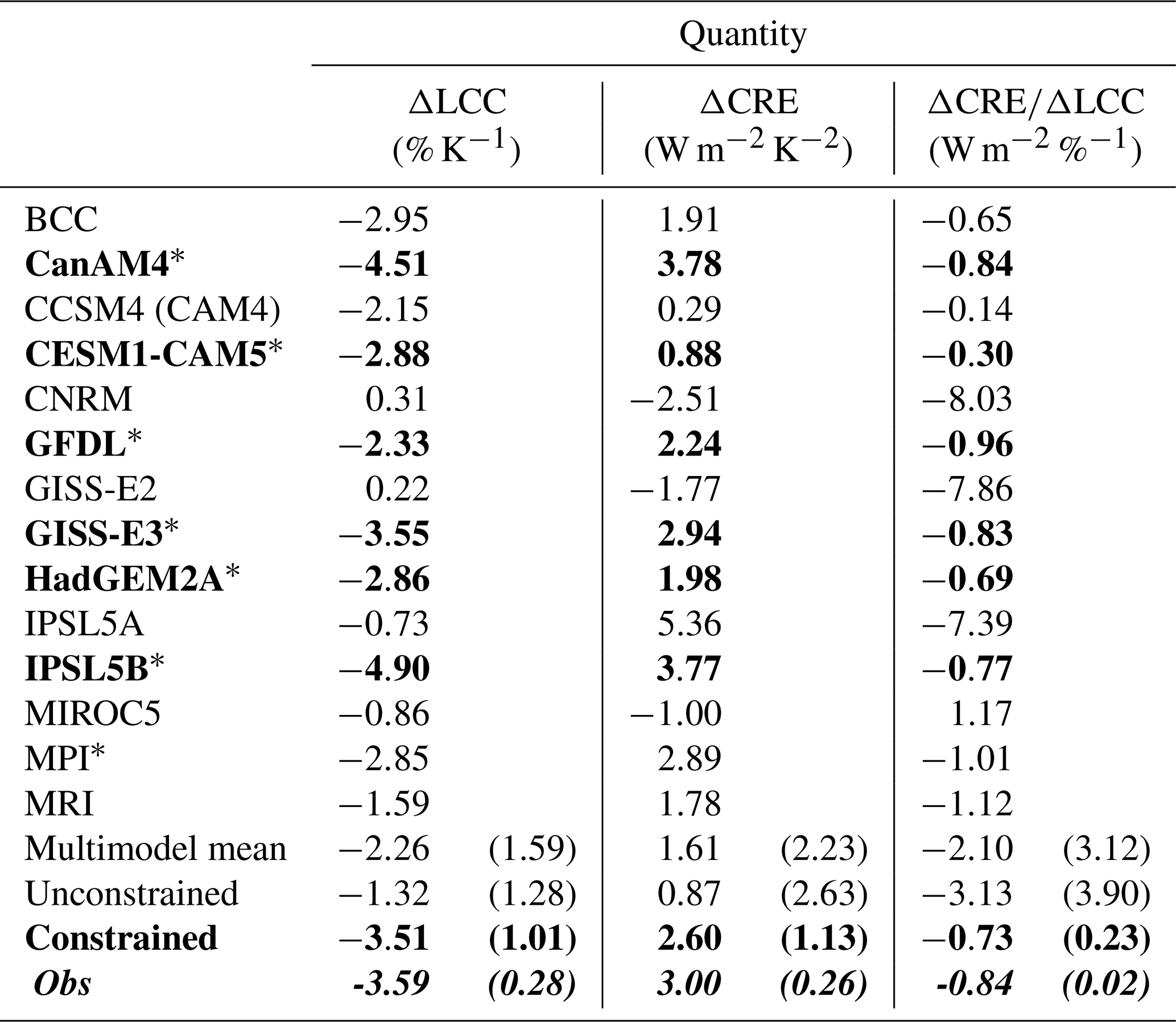
Table 2SW CRE, LCC and CRE ∕ LCC changes depending on the cloud regime for the models and the observations in subsidence regimes defined as ω500>10 hPa d−1. The bold font corresponds to the constrained models while the bold-italic font corresponds to the observations. The star means that the models include moist processes in the PBL (either due to turbulence parameterization, shallow convection or both). The numbers in parentheses correspond to the standard deviation, computed based on four different SST datasets in the observations.
4.2 Consequences for low-cloud cover
In the remainder of the paper, we use star shapes in our plots to distinguish the GISS models from the other models and emphasize the effect of cloud parameterization changes with respect to interannual LCC and cloud radiative effect changes in a GCM.
Based on this observational constraint, we now investigate how well the models simulate LCC in present-day climate and with a surface warming. Figure 1 shows the LCC maps for the observations and for the two model categories as well as their biases. Although the LCC global means of GISS models are almost identical (LCCE2=28.5 % and LCCE3=28.6 %), their spatial patterns (Fig. 1b–d) are completely different (E2 failing to produce any stratocumulus clouds), which results in a very poor correlation factor for E2 (r=0.11, the smallest of all 14 models) as opposed to a very good one for E3 (r=0.86, the largest of all 14 models). The reader should also bear in mind that E3 cloud fraction and cloud cover are slightly underestimated in the present study because the simulator is run offline (at daily frequency), which generates lower cloud fractions and cloud covers than the inline version (not shown). The constrained models (Fig. 1h) simulate larger LCC global (and tropical) means (LCC=30.5 %, r=0.92), closer to the observations (LCC=37 %), and also better reproduce the observed LCC pattern than the unconstrained models (Fig. 1j; LCC=25.7 %, r=0.86) and the multimodel mean (Fig. 1f; LCC=27.8 %, r=0.90).
We apply the same method as in Sect. 3.2 to calculate the interannual change in LCC per K of surface warming (Fig. 3a and Table 2 first column, ΔLCC∕ΔSST). Consistent with the cloud fraction profiles, GISS-E3, the only model being within the observation uncertainty, predicts a decrease in the LCC in response to a local 1 K surface warming (−3.55 % K−1), like most models (12 out of 14), as opposed to a small increase for GISS-E2 (0.22 % K−1). As the difference between GISS-E2 and E3, the multimodel spread is significantly large (5.4 % K−1, Table 2), which is about 2.5 times greater than the absolute value of the multimodel mean (−2.25 % K−1, Table 2). However, the constrained models simulate a ΔLCC∕ΔSST slightly smaller than the observation but within the observational uncertainty (−3.59 % K−1 ± 0.28 % K−1) and with a much-reduced spread (−3.49 % K−1 ± 1.01 % K−1). The observed ΔLCC∕ΔSST is significant as its amplitude is more than 3 times larger than the LCC annual standard deviation in the same dynamical regimes (1 % K−1).
It is plausible to think that ΔLCC could depend on the initial amount of LCC in a model (e.g., Brient and Bony, 2012). While the difference between GISS-E2 and GISS-E3 is not substantial, comparing this relationship for multiple versions of the GISS-E3 model (run along the course of its development) supports a relationship between ΔLCC and the present-day LCC in subsidence regions (Fig. 3b). This relationship holds regardless of whether the simulator is used or not. Except for MIROC5, which simulates a present-day LCC almost as large as the observations, the constrained models simulate a larger present-day LCC in subsidence regions (consistent with what was found in Fig. 2). When MIROC5 is set aside, the correlation between the LCC and ΔLCC in Fig. 3a becomes more obvious ( vs. for all models). One should note that the present-day LCC could be biased low in some models, due to a too-strong shielding effect by overlying high clouds compared to the observations, possibly affecting the relationship between the present-day LCC and ΔLCC. In the GISS-E3 model, the simulator does not affect ΔLCC (Fig. 3b; compare red and black versions of the same symbols), despite its significant impact on the present-day LCC as hypothesized before. In addition, the relationship may be different depending on the type of clouds, since Fig. 3 does not separate trade cumulus from stratocumulus. The explanation of the MIROC5 behavior is twofold. First, similar to the other unconstrained models, MIROC5 evidently lacks the model physics to produce Sc-type clouds, i.e., simulating moist processes in the PBL in which stratiform clouds maintain the turbulent mixing that sustains them. As a result, its ΔLCC∕ΔSST is small. Second, MIROC5 suffers from an insufficient vertical mixing of the humid air in the PBL and the dry air in the free troposphere (Ogura et al., 2017; Tatebe et al., 2018), which generates too large of an LCC over trade-wind regions compared to CALIPSO-GOCCP (not shown) and the largest mean LCC among the models. In addition, this poor vertical mixing may also explain the small amplitude of ΔLCC∕ΔSST because SST changes poorly propagate through the PBL to the free troposphere (consistent with what found by Sherwood et al., 2014).

Figure 4Relationship between the ΔLCC∕ΔSST (x axis, % K−1) and the ΔCRE∕ΔSST (y axis, W m−2 K−1) for the SW (a), the LW (b) and the net (c) radiation. The solid black line represents the linear regression of the models. The blue shading means a cloud cooling effect as opposed to red shading for a cloud warming effect.
4.3 Consequences for annual low-cloud feedbacks
In this section, we further examine the impact of cloud changes on the radiative budget for the same stratocumulus and stratocumulus-to-shallow-cumulus transition regions (over the tropical oceans and based on ω500) using CRE, defined as the difference between the all-sky flux minus the clear-sky flux at the TOA. Figure 4 shows the change in the SW, LW and net CRE per K of surface warming, referred to as ΔCRE∕ΔSST (i.e., dCRE ∕ dSST). A positive ΔCRE∕ΔSST implies a warming of the climate system due to clouds when the SST increases; conversely, a negative ΔCRE∕ΔSST implies a cooling effect. This quantity may be used as a proxy to characterize cloud feedbacks at the top of the atmosphere (e.g., Medeiros et al., 2015; Cesana et al., 2017). All observed ΔCRESW∕ΔSST, ΔCRELW∕ΔSST and ΔCRENET∕ΔSST are positive, a feature particularly well captured by GISS-E3, which is surprisingly good for both the SW and LW components of the interannual feedback, while GISS-E2 gets the sign of the SW component wrong. Both constrained and unconstrained multimodel means (colored triangles) get the correct sign of all three feedbacks although the sign and the magnitude of ΔCRENET∕ΔSST vary significantly among the models, mostly driven by the SW component, in agreement with previous studies (e.g., Medeiros et al., 2015; Cesana et al., 2017). Overall, the constrained models perform better than the unconstrained models for all three components, in terms of absolute value and variability. In particular, the unconstrained models largely underestimate the ΔCRESW∕ΔSST (0.73 W m−2 K−1, Table 2 second column) compared to the observations (3.05±0.28 W m−2 K−1), whereas the constrained models almost fall within the observed uncertainty (2.60 W m−2 K−1).
Because of the optical properties of their spherical droplets, low-lying warm marine clouds reflect more sunlight than the underlying ocean surface. As a result, any change in LCC should affect the CRESW at TOA and one should expect a good correlation between the two quantities, which is demonstrated in Fig. 4a, with a linear correlation coefficient of −0.94 (excluding the outlier of the calculation, IPSL5A). There is little correlation for the LW component, whereas for the net component, the correlation is also very large (), driven by the shortwave radiation and confirming its crucial role in determining the cloud feedback spread of CMIP models (e.g., Andrews et al., 2012). Once again, both the magnitude and the variability of the three components are better reproduced by the constrained category of models.
In addition, we analyzed the sensitivity of ΔCRESW to ΔLCC by simply computing the ratio between the two quantities as in Klein et al., 2017 (Table 2, third column). GISS-E2 largely overestimates the magnitude of this ratio (by a factor of 10) as do two other models (IPSL5A and CNRM) that poorly represent the climatological stratocumulus decks. On the other hand, GISS-E3 stands out among the best models and replicates the observed ratio. Like GISS-E2, the unconstrained models largely overestimate the radiative impact of an LCC loss (−3.13 W m−2 %−1) compared to the observations (−0.85 W m−2 %−1) while the constrained models reproduced the observed relationship quite well (−0.74 W m−2 %−1). The inability of the unconstrained models to simulate a sufficient amount of LCC in the present-day climate may generate a lack of outgoing SW radiation at TOA, which is compensated for by artificially increasing the reflectivity of the clouds during the tuning process in some modeling centers (e.g., Nam et al., 2012). This so-called “too few, too bright” problem may explain the particular behavior of the IPSL5A model in Fig. 4a. In this model, the SW CRE for a given LCC value is far too large compared to the observations and any other model (Fig. S4). This may be why the sensitivity of ΔCRESW to ΔLCC (ΔCRESW∕ΔLCC, Table 2) is too large and far off the correlation line in Fig. 4a. In addition, the radiative effect of the clear-sky portion of the cloudy grid boxes can amplify or dampen the interannual SW cloud feedback (ΔCRESW∕ΔSST). For example, artificially increasing the specific humidity of the clear sky in GISS-E3 (for radiative transfer only) reduces the SW CRE at TOA because of the increased SW absorption by water vapor, which ultimately dampens the positive SW cloud feedback with respect to the change in LCC per K (ΔCRESW∕ΔLCC, not shown).
The constrained models all generate large stratocumulus decks along with a substantial amount of tropical low clouds in non-stratocumulus regions, which seems key to simulating the correct global response of low clouds to surface warming. This behavior is likely due to the fact that they simulate moist processes in the PBL by either turbulence (e.g., GISS-E3, CESM1-CAM5, GFDL AM3, HadGEM2A, CanAM4), convection (IPSL5B) or both parameterizations (HadGEM2A), in addition to having stratocumulus decks. This becomes more evident when looking at the evolution of individual models. For example, implementing a more physically based moist turbulence parameterization (following Bretherton and Park, 2009) in the GISS-E3 model changes the sign of ΔLCC∕ΔSST and ΔCRESW∕ΔSST and brings the model results within the range of uncertainty of the observations. Similarly, the changes in the IPSL model from version 5A to 5B significantly improved its simulation of the ΔLCC and ΔCRESW quantities most likely because its dry PBL was effectively turned into a moist PBL through the implementation of moist shallow convection within the PBL (Rio and Hourdin, 2008), which improved their wind profiles and PBL height (Hourdin et al., 2013), combined with a revision of their turbulence scheme, which improved their representation of stratocumulus clouds. However, the MPI moist-PBL model does not fall into the constrained category. Even though its results are quite close to the observations, the clear overestimation of the cloud frequency above 2.16 km (Fig. S3, likely trade cumulus clouds) alters its ΔCF and leads to a sensitivity of ΔCREsw to ΔLCC that is too strong. Conversely, the BCC dry-PBL model captures ΔLCC and ΔCREsw variations pretty well (within the range of the constrained models) although its ΔCF is unrealistic. Therefore, the capacity of the models to replicate the observed response of low-level clouds and radiation to warmer surface temperature seems to be tied to whether or not (i) they simulate moist processes in the PBL and (ii) their turbulence scheme sustains stratocumulus clouds. Such results also demonstrate that a simple description of the cloud-top properties – i.e., as seen from space-borne passive sensors – is not sufficient to fully understand and predict how clouds may react to surface temperature forcings and further requires information on the vertical structure of clouds.
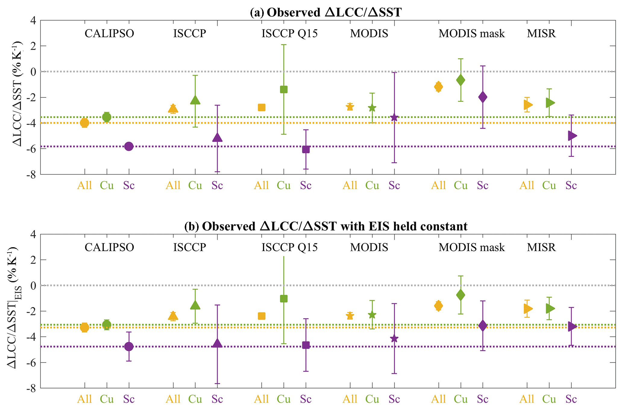
Figure 5(a) LCC change per K of SST warming (ΔLCC∕ΔSST, % K−1) per type of cloud (all clouds in orange, trade cumulus clouds in green and stratocumulus clouds in purple) for five observational datasets: CALIPSO-GOCCP (circles, 2007–2016, Cesana et al., 2016), ISCCP (triangles, 1999–2008, Rossow and Schiffer, 1999), ISCCP Q15 (squares, 1999–2008, modified to take into account the shielding effect of high clouds following Qu et al., 2015), MODIS retrieval (stars, 2003–2015, Pincus et al., 2012), MODIS mask (diamonds, 2003–2015, using partly cloudy pixels, Pincus et al., 2012) and MISR (right triangles, 2001–2012, Marchand and Ackerman, 2010). Cloud types are defined based on the subsidence regime for “all” clouds (ω500>10 hPa d−1) and further based on four regions described in Fig. S5 for the trade cumulus (Cu) and stratocumulus clouds (Sc). The uncertainty bars correspond to ± 1 standard deviation using the four SST datasets for the “all” type of cloud and to ± 1 standard deviation of the four regions for the Cu and Sc types of cloud. (b) Same as (a) but with the EIS held constant as in Qu et al. (2015) and Klein et al. (2017).
4.4 Discriminating trade cumulus from stratocumulus clouds
Given the different factors controlling cumulus and stratocumulus clouds, one could expect a different response of each type of cloud to a surface temperature perturbation. This is further supported by the diverse behavior of modeled ΔLCC∕ΔSST, which is correlated with the ability of the models to produce or not produce a large amount of stratocumulus in the present climate. To verify this, we determine the ΔLCC∕ΔSST of trade-cumulus- (ΔLCCCu∕ΔSST) and stratocumulus-dominated regions (ΔLCCSc∕ΔSST) and their associated ΔCRESW∕ΔSST.
Distinguishing cumulus from stratocumulus clouds is particularly challenging in the observations. Climatologically the two cloud types can be separated using k-means clustering of optical-thickness–cloud-top-pressure histograms over GCM grid-sized areas (Chen and Del Genio, 2009), although instantaneous errors can arise, e.g., from overlying clouds. In the PBL, as the inversion strength increases, the moisture tends to increase, leading to larger cloud fractions (e.g., Klein and Hartmann, 1993). This phenomenon explains why lower-tropospheric stability (LTS), defined as the difference between potential temperature at 700 mbar and the surface, is well correlated with LCC in the observations over the tropical oceans (e.g., Klein and Hartmann, 1993; Wood and Bretherton, 2006). We verified this relationship using LTS derived from the ERA-Interim reanalysis and CALIPSO-GOCCP LCC. The correlation between the two quantities is 0.65 but decreases when limited to larger LTS values (0.51 for LTS>15 K, 0.38 for LTS>17 K). We tried to use LTS-based thresholds to separate stratocumulus decks from other low-level clouds but the method does not work well for monthly climatology (not shown). Besides, only a few models have high LTS–LCC correlations (4 out of 14 are larger than 0.6), and for those, the larger LTS does not match the stratocumulus areas. This is somewhat consistent with the decoupling of the LTS and SST pointed out by Su et al. (2013). Using estimated inversion strength – an LCC predictor that can be also used at midlatitudes (Wood and Bretherton, 2006) – rather than LTS gives even better correlations in both the observations (see Fig. 5) and E3. However, we could only compute the LTS with the output available from other models. Note that using convective and stratiform cloud fraction (often separated in GCMs) would solve this problem on the model side but such partitioning is not provided in the CMIP5 archive.
Instead, we focus on eight specific regions (Fig. S5) that have been identified as being dominated by either stratocumulus clouds or trade cumulus clouds in previous studies (e.g., McCoy et al., 2017). This method does not allow a model evaluation as the models may not be able to simulate the correct type of clouds in these regions, regardless of their ability to reproduce the response of each type of cloud to SST variability. Therefore we focus our analysis on observations only. In the literature, all studies referenced before except for Brient and Schneider (2016) exclusively used passive sensors to derive ΔLCC∕ΔSST composites. In contrast, we use CALIPSO-GOCCP, which has a shorter time record and poorer sampling but a greater sensitivity to trade cumulus clouds due to both its narrower horizontal footprint and its better instrument sensitivity to liquid cloud particles. However, because we are using different methods and regions in our study, we included two International Satellite Cloud Climatology Project (ISCCP) estimates (Qu et al., 2015; Pincus et al., 2012), two Moderate Resolution Imaging Spectroradiometer (MODIS) estimates (Pincus et al., 2012) and one Multiangle Imaging Spectroradiometer (MISR) estimate (Marchand et al., 2010) of ΔLCC∕ΔSST for comparison. For this comparison, both night- and daytime CALIPSO-GOCCP data are used to maximize the sample size and all datasets are reprojected onto a 2.5∘ × 2.5∘ grid. The original ISCCP dataset is the same used by Pincus et al. (2012), a GCM-oriented ISCCP dataset prepared to facilitate the evaluation of GCMs (consistent with the ISCCP simulator) based on a subset of ISCCP variables (Rossow and Schiffer, 1999). The second ISCCP dataset, so-called ISCCP Q15, is derived from the first one. A correction for possible masking effect of overlying clouds is applied as in Qu et al. (2015): , where LCC, M and H are the original low-cloud cover, the mid-cloud cover and the high-cloud cover, respectively. Those can be interpreted as low and high uncertainty estimates. Using GISS-E3 and the ISCCP simulator, we found that the corrected LCC′ out of the ISCCP simulator is slightly overestimated compared to the original model LCC although the two quantities are highly correlated (see Fig. S6). We excluded data before 1999 (April 1999 to March 2008, 10 years as for CALIPSO-GOCCP) due to artifacts in the dataset. Similarly, the MODIS datasets combine observations from the MODIS Terra and Aqua platforms for model evaluation (also consistent with the MODIS simulator). The daily collection 5.1 files are monthly averaged and a subset of relevant variables are saved. The first dataset includes the cloud fraction from cloud retrievals, which are the cloud fraction used to derive MODIS cloud properties in the collection 5.1 product. These are pixels that are entirely filled with clouds. On the other hand, the second dataset contains the cloud fraction from the so-called MODIS mask, which includes partially cloud-filled pixels (Pincus et al., 2012; Platnick et al., 2003). Here we used 13 years of data from 2003 to 2015 (overlapping period between Aqua and Terra platforms). The MISR dataset provides particularly accurate height retrievals by taking advantage of its stereo-imaging technique and is less sensitive to high clouds than instruments used in MODIS and ISCCP datasets, which brings a complementary passive-sensor view of LCC distributions (Marchand et al., 2010). Similar to ISCCP and MODIS, the MISR dataset used in this analysis was designed for model-evaluation purposes (Marchand and Ackerman, 2010). LCC is derived from 12 years (2001–2012) of data by adding cloud fractions from 500 to 3000 m (note that the level 0–500 m was excluded due to the presence of an undetermined artifact).
Table 3CRE, LCC and CRE/LCC changes depending on the type of clouds for the different observational datasets used in the study. Note that for CALIPSO-GOCCP night- and daytime are used, contrary to Table 2.
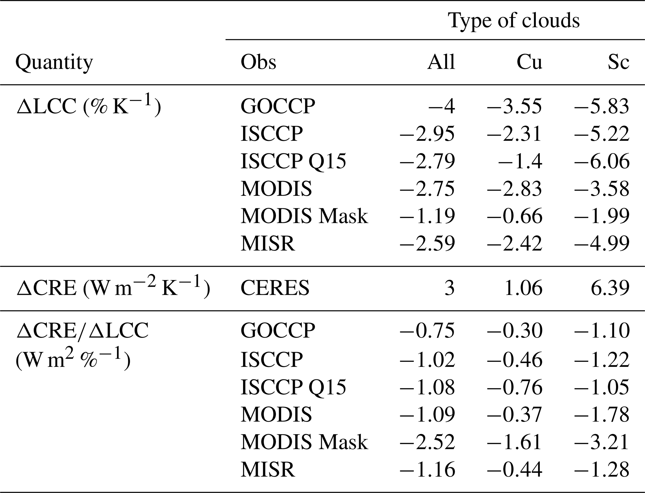
Figure 5 shows the ΔLCC∕ΔSSTs for all datasets using the same cloud regimes based on ω500 and the same four trade-cumulus- and four stratocumulus-dominated regions (Fig. S5). Consistent with previous studies (e.g., McCoy et al., 2017; Myers and Norris, 2017; Qu et al., 2015), all datasets agree on a decrease in the LCC for increasing SSTs. The decrease still occurs but to a smaller extent (∼20 % smaller) when the EIS, another supposed low-cloud-controlling factor, is held constant (see Klein et al., 2017). The overall magnitude of the change is larger in CALIPSO (−4 % K−1) than in the passive-sensor datasets (−1.19 to 2.95 % K−1, Table 3) regardless of the SST dataset used (Fig. S7). When only the stratocumulus regions are considered, all datasets show a larger decrease in the LCC than for the trade cumulus clouds or all tropical low clouds. This may suggest that the overall behavior of clouds is controlled by the Cu and Sc-Cu transitioning clouds (i.e., Bony and Dufresne, 2005), which supposedly cover a larger area of the tropics, although it does not guarantee it as we do not know for sure what type of clouds cover what part of the tropics from the observations. The difference between ISCCP, MISR and GOCCP is also relatively smaller in Sc regions ( % K−1 vs. and −6.06 % K−1 for the two ISSCP products described above and % K−1) than in the Cu regions ( % K−1 vs. and −1.4 % K−1 and % K−1, Table 3). Without the region of the east coast of Peru, MODIS observations also agree well with ISCCP, MISR and GOCCP ΔLCCSc (within 15 %, not shown) although the MODIS mask cloud cover remains smaller for the most part than all other datasets regardless of the regions selected.
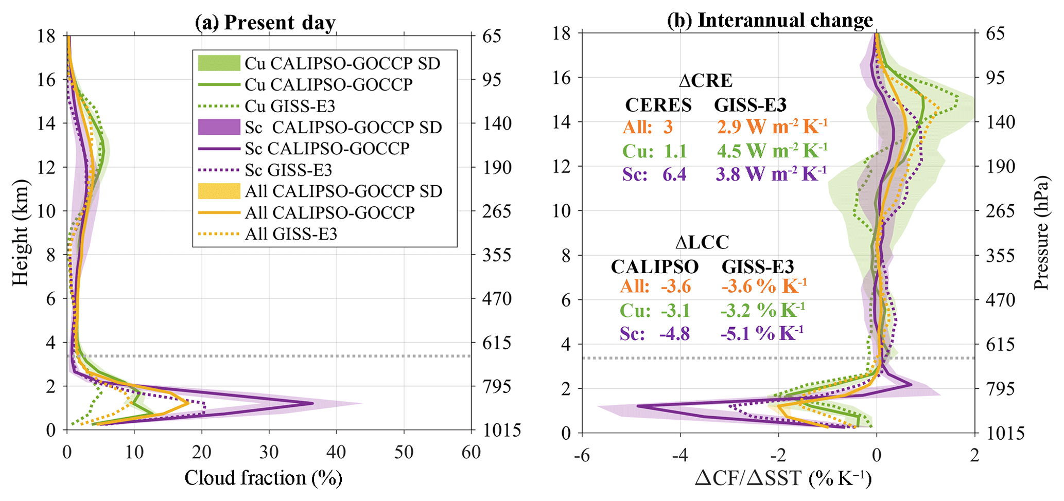
Figure 6(a) Vertical profiles (height in km, y axis) of cloud fraction (CF in %, x axis) and (b) interannual cloud fraction change due to SST variations (ΔCF∕ΔSST in % K−1, x axis) as observed by CALIPSO-GOCCP observations for the three types of cloud: all clouds in orange, trade cumulus clouds (Cu) in green and stratocumulus clouds (Sc) in purple. The shading areas correspond to the standard deviation using the four SST datasets for the “all” type of cloud and to the standard deviation of the four regions for the Cu and Sc types of cloud. The horizontal dotted line denotes the height (3.36 km) used to define the low-cloud cover in CALIPSO-GOCCP.
Finally, it is also worth mentioning that the sensitivity of CRE at TOA per unit change in cloud fraction is significantly smaller in magnitude for trade cumulus clouds than for stratocumulus clouds in the four satellite estimates, including CALIPSO-GOCCP (−0.30 W m−2 %−1 vs. −1.10 W m−2 %−1), consistent with the fact that trade cumulus clouds are less reflective than stratocumulus clouds (Table 3). Even though differences in TOA CRE would emerge if one could use CERES-like observations at the CALIPSO horizontal resolution, these biases would remain small (e.g., Ham et al., 2015). In addition, we document the cloud opacity in the two regions using the ratio of opaque cloud cover (fully attenuating the lidar, Guzman et al., 2017) to the total cloud cover, Ropacity. We find that the stratocumulus Ropacity (75.9 %) is 50 % larger than that of trade cumulus regions (50.6 %), confirming the larger optical thickness of clouds in the stratocumulus regions than in the trade cumulus regions. Overall, all passive-sensor estimates of this quantity are larger in magnitude than that of CALIPSO-GOCCP (−0.75 W m−2 %−1 vs. −1.02 to −2.52 W m−2 %−1, Table 3), even more so in the trade cumulus regions.
The vertical response of the CF to a surface warming (ΔCFall, ΔCFSc, ΔCFCu) is shown in Fig. 6b. In the observations, the low-cloud top is lifted up coincident with a large decrease in cloud fraction below in stratocumulus regions (purple line) while, in the trade cumulus regions, the cloud top does not change and the decrease is significantly smaller (green line). Note that because our Sc and Cu are defined by regions rather than actual cloud types, we cannot distinguish between an actual rising of Sc cloud tops and a transition from lower-topped Sc to higher-topped Cu; both may contribute to the behavior of the ΔCFSc profile. Depending on low-level cloud-top height and the type of cloud, the effect of a surface warming is therefore different, generating a small decrease for “higher” low-level clouds (Cu) as compared to a larger decrease in the “lower” low-level clouds (Sc) along with an increase in their cloud-top height. Thus, favoring one cloud type over the other in the models may result in either an overestimate (too many Sc) or an underestimate of the ΔLCC∕ΔSST (too many Cu). Because the overall ΔLCC∕ΔSST and the height of the CF change (Fig. 2) are underestimated by most models, it is likely that models do not simulate enough stratocumulus clouds. We also investigate how well GISS-E3, a model that can produce a decent spatial pattern and amount of low clouds as well as a correct ΔCF, performs against the observations. GISS-E3 ΔCFCu (green dotted line) is quite well captured by GISS-E3, whereas ΔCFSc (purple dotted line) is underestimated (its magnitude being out of the observed SD) and the Sc cloud-top lifting is not reproduced. The overall ΔCF (orange dotted line) peaks slightly too high with a too-small magnitude compared to the observations. Therefore, GISS-E3 likely underestimates the amount of Sc clouds compared to Cu, supporting the aforementioned hypothesis, in addition to slightly underestimating the amount of all types of clouds in the present-day climate (Fig. 6a). The good agreement of the total ΔCREsw with the observations results from compensating errors between an overestimated Cu ΔCREsw and underestimated Sc ΔCREsw although the corresponding ΔLCCs are well simulated. This suggests that the regional GISS-E3 radiative effect of low clouds is likely not well captured, in accordance with a long-standing problem in GCMs (e.g., Nam et al., 2012).
In response to interannual surface warming, the marine tropical low-cloud cover (LCC) as observed by the active sensor from the CALIPSO satellite over a 10-year period significantly decreases ( % K−1). This reduction of the LCC is larger than that found using results from passive-sensor satellites ( to −2.95 % K−1), albeit consistent in terms of sign and magnitude (e.g., McCoy et al., 2017; Qu et al., 2015; Seethala et al., 2015). Overall, the ensemble mean of CMIP5 models captures the sign and the shape of the observed interannual low-cloud cover change (ΔLCC∕ΔSST) quite well. However, its magnitude is underestimated and the model variability is large ( % K−1), with some models (2 out of 14) even producing the wrong sign (a gain instead of a loss).
When scrutinized as a function of height, the interannual cloud fraction change (ΔCF∕ΔSST) in the lower levels reveals various behaviors, which depend on the type of cloud and its height. We further show that it is possible to separate the model responses to SST variations using CALIPSO observations of the vertical cloud fraction (ΔCF∕ΔSST) as a constraint: we select the GCMs that produce the most realistic change in cloud profile per K of SST warming, referred to as constrained models. By doing so, we find that the constrained models, including the latest version of the GISS model (GISS-E3), simulate a more realistic behavior of low-level cloud fraction and their associated interannual radiative feedbacks (ΔCRESW∕ΔSST) together with a smaller variability in response to a surface warming. Their averaged ΔLCC∕ΔSST is within the observed uncertainty while they slightly underestimate the ΔCRESW∕ΔSST. Meanwhile, the unconstrained category, which includes the CMIP5 version of the GISS model (GISS-E2), fails to reproduce the observed magnitude of both quantities by a factor of 3 to 4. The fact that models that simulate moist processes within the PBL produce sustainable stratocumulus decks appears crucial to replicate the observed relationship between cloud, radiation and surface temperature.
Separating clouds between stratocumulus and trade cumulus categories helps us better quantify their contribution to global tropical low-level cloud change. The vertical structure of the change is indeed different in regions dominated by stratocumulus clouds compared to those dominated by cumulus clouds. Over the stratocumulus regions, the cloud top increases slightly, accompanied by a large decrease in the cloud fraction below, whereas over the trade cumulus regions, cloud fraction decreases to a smaller degree, but over its full vertical extent. As a result, the cloud cover change per unit SST change is smaller over trade cumulus regions than over stratocumulus regions ( % K−1 compared to % K−1). Passive-sensor observations confirm this result, although their overall ΔLCC∕ΔSST is consistently smaller regardless of the SST dataset used (Fig. S7), mostly attributable to trade cumulus regions where passive sensors are less sensitive to broken cumulus. However, the derived slopes for trade cumulus and stratocumulus from active and passive methods are within the measurement uncertainty and cannot formally be distinguished (Fig. S7).
Finally, a region-based evaluation of the GISS-E3 model suggests that producing realistic global ΔCF, ΔLCC and ΔCRE may be the result of compensating errors between the Sc-dominated and Cu-dominated regions. However, it is difficult to determine with certainty whether the model is biased or not as we discriminate these cloud types by regions and not by actual type with the method used in this study. Future work will focus on developing a method to discriminate stratocumulus from trade cumulus clouds in satellite-based observations. By doing so, we will be able to assess the spatial distributions of these clouds and to evaluate the models more precisely. In addition, refining the contribution of additional cloud-controlling factors may advance our understanding of physical processes driving the change in cloud fraction in response to a warming climate.
The GISS-E3 simulations can be made available upon request; the final version of GISS-E3 will be made part of the CMIP6 model archive. The CMIP5 simulations were downloaded from the World Data Center for Climate (WDCC) website (http://cera-www.dkrz.de/, last access: December 2016). CALIPSO-GOCCP, part of MISR and ISCCP observations were downloaded from the CFMIP-OBS website (http://climserv.ipsl.polytechnique.fr/cfmip-obs/Calipso_goccp.html, last access: December 2016). CERES-EBAF 4.0 TOA fluxes were downloaded on the CERES website (https://ceres.larc.nasa.gov/, last access: December 2016). The ERA-Interim dataset was downloaded from ClimServ (http://climserv.ipsl.polytechnique.fr/, last access: December 2016). MODIS data were obtained from https://ladsweb.modaps.eosdis.nasa.gov/archive/NetCDF/L3_Monthly/ (last access: December 2016). The NOAA-OI v2, COBE-SST2 and ERSST v5 datasets were provided by the NOAA/OAR/ESRL PSD, Boulder, Colorado, USA, from their website (https://www.esrl.noaa.gov/psd/, last access: December 2016).
The supplement related to this article is available online at: https://doi.org/10.5194/acp-19-2813-2019-supplement.
GC and AD designed the study and GC carried out the analysis. AD, AA, GE, MK, AF, YC and MSY developed the model code and GC performed the simulations. GC wrote the manuscript with contributions from all co-authors.
The authors declare that they have no conflict of interest.
Gregory Cesana and Anthony D. Del Genio
were supported by a CloudSat–CALIPSO grant at the NASA Goddard
Institute for Space Studies. Andrew S. Ackerman, Maxwell Kelley, Ye Cheng, Mao-Sung Yao, and
Ann M. Fridlind were supported by NASA Modeling, Analysis, and Prediction Program grants. The authors acknowledge the
World Climate Research Programme's Working Group on Coupled Modeling, which
is responsible for CMIP, and thank the climate modeling groups for producing
and making available their model output. Gregory Cesana would like to thank Tim Myers
for assistance on the computation of EIS and statistical relationships,
Steve Klein and Robert Pincus for helpful discussions on the topic, Roj
Marchand for his help in handling MISR data and Catherine Rio for her help
in interpreting the IPSL models' results. Finally, the authors thank
Johannes Quaas for editing the manuscript and the two anonymous reviewers
for their helpful comments.
Edited by: Johannes Quaas
Reviewed by: two anonymous referees
Abdella, K. and McFarlane, N. A.: Parameterization of the surface-layer exchange coefficients for atmospheric models, Bound.-Lay. Meteorol., 80, 223–248, https://doi.org/10.1007/BF00119544, 1996.
Andrews, T., Gregory, J. M., Webb, M. J., and Taylor, K. E.: Forcing, feedbacks and climate sensitivity in CMIP5 coupled atmosphere-ocean climate models: Climate sensitivity in CMIP5 models, Geophys. Res. Lett., 39, L09712, https://doi.org/10.1029/2012GL051607, 2012.
Anon: The New GFDL Global Atmosphere and Land Model AM2-LM2: Evaluation with Prescribed SST Simulations, J. Climate, 17, 4641–4673, https://doi.org/10.1175/JCLI-3223.1, 2004.
Bodas-Salcedo, A., Webb, M. J., Bony, S., Chepfer, H., Dufresne, J.-L., Klein, S. A., Zhang, Y., Marchand, R., Haynes, J. M., Pincus, R., and John, V. O.: COSP: Satellite simulation software for model assessment, B. Am. Meteorol. Soc., 92, 1023–1043, https://doi.org/10.1175/2011BAMS2856.1, 2011.
Bony, S. and Dufresne, J.-L.: Marine boundary layer clouds at the heart of tropical cloud feedback uncertainties in climate models, Geophys. Res. Lett., 32, L20806, https://doi.org/10.1029/2005GL023851, 2005.
Bretherton, C. S.: Insights into low-latitude cloud feedbacks from high-resolution models, Philos. T. R. Soc. A., 373, 20140415, https://doi.org/10.1098/rsta.2014.0415, 2015.
Bretherton, C. S. and Park, S.: A New Moist Turbulence Parameterization in the Community Atmosphere Model, J. Climate, 22, 3422–3448, https://doi.org/10.1175/2008JCLI2556.1, 2009.
Bretherton, C. S., Blossey, P. N., and Jones, C. R.: Mechanisms of marine low cloud sensitivity to idealized climate perturbations: A single-LES exploration extending the CGILS cases: Les of boundary-layer cloud feedback, J. Adv. Model Earth Sy., 5, 316–337, https://doi.org/10.1002/jame.20019, 2013.
Brient, F. and Bony, S.: How may low-cloud radiative properties simulated in the current climate influence low-cloud feedbacks under global warming?: Low cloud feedback, Geophys. Res. Lett., 39, L20807, https://doi.org/10.1029/2012GL053265, 2012.
Brient, F. and Schneider, T.: Constraints on Climate Sensitivity from Space-Based Measurements of Low-Cloud Reflection, J. Climate, 29, 5821–5835, https://doi.org/10.1175/JCLI-D-15-0897.1, 2016.
Brient, F., Schneider, T., Tan, Z., Bony, S., Qu, X., and Hall, A.: Shallowness of tropical low clouds as a predictor of climate models' response to warming, Clim. Dynam., 47, 433–449, https://doi.org/10.1007/s00382-015-2846-0, 2016.
Brinkop, S. and Roeckner, E.: Sensitivity of a general circulation model to parameterizations of cloud-turbulence interactions in the atmospheric boundary layer, Tellus A, 47, 197–220, https://doi.org/10.1034/j.1600-0870.1995.t01-1-00004.x, 1995.
Brown, A. R., Beare, R. J., Edwards, J. M., Lock, A. P., Keogh, S. J., Milton, S. F., and Walters, D. N.: Upgrades to the Boundary-Layer Scheme in the Met Office Numerical Weather Prediction Model, Bound.-Lay. Meteorol., 128, 117–132, https://doi.org/10.1007/s10546-008-9275-0, 2008.
Caldwell, P. M., Zelinka, M. D., and Klein, S. A.: Evaluating Emergent Constraints on Equilibrium Climate Sensitivity, J. Climate, 31, 3921–3942, https://doi.org/10.1175/JCLI-D-17-0631.1, 2018.
Cesana, G. and Chepfer, H.: How well do climate models simulate cloud vertical structure? A comparison between CALIPSO-GOCCP satellite observations and CMIP5 models: Evaluation of clouds in cmip5 models, Geophys. Res. Lett., 39, L20803, https://doi.org/10.1029/2012GL053153, 2012.
Cesana, G. and Waliser, D. E.: Characterizing and understanding systematic biases in the vertical structure of clouds in CMIP5/CFMIP2 models: Vertical Structure of Clouds, Geophys. Res. Lett., 43, 10538–10546, https://doi.org/10.1002/2016GL070515, 2016.
Cesana, G., Chepfer, H., Winker, D., Getzewich, B., Cai, X., Jourdan, O., Mioche, G., Okamoto, H., Hagihara, Y., Noel, V., and Reverdy, M.: Using in situ airborne measurements to evaluate three cloud phase products derived from CALIPSO: CALIPSO Cloud Phase Validation, J. Geophys. Res.-Atmos., 121, 5788–5808, https://doi.org/10.1002/2015JD024334, 2016.
Cesana, G., Suselj, K., and Brient, F.: On the Dependence of Cloud Feedbacks on Physical Parameterizations in WRF Aquaplanet Simulations: WRF Aquaplanet Cloud Feedbacks, Geophys. Res. Lett., 44, 10762–10771, https://doi.org/10.1002/2017GL074820, 2017.
Chen, Y. and Del Genio, A. D.: Evaluation of tropical cloud regimes in observations and a general circulation model, Clim. Dynam., 32, 355–369, https://doi.org/10.1007/s00382-008-0386-6, 2009.
Chepfer, H., Bony, S., Winker, D., Chiriaco, M., Dufresne, J.-L., and Sèze, G.: Use of CALIPSO lidar observations to evaluate the cloudiness simulated by a climate model, Geophys. Res. Lett., 35, L15704, https://doi.org/10.1029/2008GL034207, 2008.
Chepfer, H., Cesana, G., Winker, D., Getzewich, B., Vaughan, M., and Liu, Z.: Comparison of Two Different Cloud Climatologies Derived from CALIOP-Attenuated Backscattered Measurements (Level 1): The CALIPSO-ST and the CALIPSO-GOCCP, J. Atmos. Ocean. Tech., 30, 725–744, https://doi.org/10.1175/JTECH-D-12-00057.1, 2013.
Dee, D. P., Uppala, S. M., Simmons, A. J., Berrisford, P., Poli, P., Kobayashi, S., Andrae, U., Balmaseda, M. A., Balsamo, G., Bauer, P., Bechtold, P., Beljaars, A. C. M., van de Berg, L., Bidlot, J., Bormann, N., Delsol, C., Dragani, R., Fuentes, M., Geer, A. J., Haimberger, L., Healy, S. B., Hersbach, H., Hólm, E. V., Isaksen, L., Kållberg, P., Köhler, M., Matricardi, M., McNally, A. P., Monge-Sanz, B. M., Morcrette, J.-J., Park, B.-K., Peubey, C., de Rosnay, P., Tavolato, C., Thépaut, J.-N., and Vitart, F.: The ERA-Interim reanalysis: configuration and performance of the data assimilation system, Q. J. Roy. Meteor. Soc., 137, 553–597, https://doi.org/10.1002/qj.828, 2011.
Del Genio, A. D., Yao, M.-S., Kovari, W., and Lo, K. K.-W.: A Prognostic Cloud Water Parameterization for Global Climate Models, J. Climate, 9, 270–304, https://doi.org/10.1175/1520-0442(1996)009<0270:APCWPF>2.0.CO;2, 1996.
Del Genio, A. D., Kovari, W., Yao, M.-S., and Jonas, J.: Cumulus Microphysics and Climate Sensitivity, J. Climate, 18, 2376–2387, https://doi.org/10.1175/JCLI3413.1, 2005.
Del Genio, A. D., Wu, J., Wolf, A. B., Chen, Y., Yao, M.-S., and Kim, D.: Constraints on Cumulus Parameterization from Simulations of Observed MJO Events, J. Climate, 28, 6419–6442, https://doi.org/10.1175/JCLI-D-14-00832.1, 2015.
de Szoeke, S. P., Verlinden, K. L., Yuter, S. E., and Mechem, D. B.: The Time Scales of Variability of Marine Low Clouds, J. Climate, 29, 6463–6481, https://doi.org/10.1175/JCLI-D-15-0460.1, 2016.
Donner, L. J., Wyman, B. L., Hemler, R. S., Horowitz, L. W., Ming, Y., Zhao, M., Golaz, J.-C., Ginoux, P., Lin, S.-J., Schwarzkopf, M. D., Austin, J., Alaka, G., Cooke, W. F., Delworth, T. L., Freidenreich, S. M., Gordon, C. T., Griffies, S. M., Held, I. M., Hurlin, W. J., Klein, S. A., Knutson, T. R., Langenhorst, A. R., Lee, H.-C., Lin, Y., Magi, B. I., Malyshev, S. L., Milly, P. C. D., Naik, V., Nath, M. J., Pincus, R., Ploshay, J. J., Ramaswamy, V., Seman, C. J., Shevliakova, E., Sirutis, J. J., Stern, W. F., Stouffer, R. J., Wilson, R. J., Winton, M., Wittenberg, A. T., and Zeng, F.: The Dynamical Core, Physical Parameterizations, and Basic Simulation Characteristics of the Atmospheric Component AM3 of the GFDL Global Coupled Model CM3, J. Climate, 24, 3484–3519, https://doi.org/10.1175/2011JCLI3955.1, 2011.
Elsaesser, G. S., Del Genio, A. D., Jiang, J. H., and van Lier-Walqui, M.: An Improved Convective Ice Parameterization for the NASA GISS Global Climate Model and Impacts on Cloud Ice Simulation, J. Climate, 30, 317–336, https://doi.org/10.1175/JCLI-D-16-0346.1, 2017.
Galperin, B., Kantha, L. H., Hassid, S., and Rosati, A.: A Quasi-equilibrium Turbulent Energy Model for Geophysical Flows, J. Atmos. Sci., 45, 55–62, https://doi.org/10.1175/1520-0469(1988)045<0055:AQETEM>2.0.CO;2, 1988.
Geoffroy, M.-C., Côté, S. M., Giguère, C.-É., Dionne, G., Zelazo, P. D., Tremblay, R. E., Boivin, M., and Séguin, J. R.: Closing the gap in academic readiness and achievement: the role of early childcare: Childcare, socioeconomic background, and academic readiness and achievement, J. Child Psychol. Psyc., 51, 1359–1367, https://doi.org/10.1111/j.1469-7610.2010.02316.x, 2010.
Gettelman, A. and Morrison, H.: Advanced Two-Moment Bulk Microphysics for Global Models. Part I: Off-Line Tests and Comparison with Other Schemes, J. Climate, 28, 1268–1287, https://doi.org/10.1175/JCLI-D-14-00102.1, 2015.
Guzman, R., Chepfer, H., Noel, V., Vaillant de Guélis, T., Kay, J. E., Raberanto, P., Cesana, G., Vaughan, M. A., and Winker, D. M.: Direct atmosphere opacity observations from CALIPSO provide new constraints on cloud-radiation interactions: GOCCP v3.0 OPAQ Algorithm, J. Geophys. Res.-Atmos., 122, 1066–1085, https://doi.org/10.1002/2016JD025946, 2017.
Ham, S.-H., Kato, S., Barker, H. W., Rose, F. G., and Sun-Mack, S.: Improving the modelling of short-wave radiation through the use of a 3-D scene construction algorithm: Improving Short-Wave Radiation Modelling by SCA, Q. J. Roy. Meteor. Soc., 141, 1870–1883, https://doi.org/10.1002/qj.2491, 2015.
Hirahara, S., Ishii, M., and Fukuda, Y.: Centennial-Scale Sea Surface Temperature Analysis and Its Uncertainty, J. Climate, 27, 57–75, https://doi.org/10.1175/JCLI-D-12-00837.1, 2014.
Holtslag, A. A. M. and Boville, B. A.: Local Versus Nonlocal Boundary-Layer Diffusion in a Global Climate Model, J. Climate, 6, 1825–1842, https://doi.org/10.1175/1520-0442(1993)006<1825:LVNBLD>2.0.CO;2, 1993.
Hourdin, F., Musat, I., Bony, S., Braconnot, P., Codron, F., Dufresne, J.-L., Fairhead, L., Filiberti, M.-A., Friedlingstein, P., Grandpeix, J.-Y., Krinner, G., LeVan, P., Li, Z.-X., and Lott, F.: The LMDZ4 general circulation model: climate performance and sensitivity to parametrized physics with emphasis on tropical convection, Clim. Dynam., 27, 787–813, https://doi.org/10.1007/s00382-006-0158-0, 2006.
Hourdin, F., Grandpeix, J.-Y., Rio, C., Bony, S., Jam, A., Cheruy, F., Rochetin, N., Fairhead, L., Idelkadi, A., Musat, I., Dufresne, J.-L., Lahellec, A., Lefebvre, M.-P., and Roehrig, R.: LMDZ5B: the atmospheric component of the IPSL climate model with revisited parameterizations for clouds and convection, Clim. Dynam., 40, 2193–2222, https://doi.org/10.1007/s00382-012-1343-y, 2013.
Huang, B., Thorne, P. W., Banzon, V. F., Boyer, T., Chepurin, G., Lawrimore, J. H., Menne, M. J., Smith, T. M., Vose, R. S., and Zhang, H.-M.: Extended Reconstructed Sea Surface Temperature, Version 5 (ERSSTv5): Upgrades, Validations, and Intercomparisons, J. Climate, 30, 8179–8205, https://doi.org/10.1175/JCLI-D-16-0836.1, 2017.
Kärcher, B.: A parameterization of cirrus cloud formation: Homogeneous freezing of supercooled aerosols, J. Geophys. Res., 107, https://doi.org/10.1029/2001JD000470, 2002.
Klein, S. A. and Hartmann, D. L.: The Seasonal Cycle of Low Stratiform Clouds, J. Climate, 6, 1587–1606, https://doi.org/10.1175/1520-0442(1993)006<1587:TSCOLS>2.0.CO;2, 1993.
Klein, S. A. and Jakob, C.: Validation and Sensitivities of Frontal Clouds Simulated by the ECMWF Model, Mon. Weather Rev., 127, 2514–2531, https://doi.org/10.1175/1520-0493(1999)127<2514:VASOFC>2.0.CO;2, 1999.
Klein, S. A. and Hall, A.: Emergent Constraints for Cloud Feedbacks, Current Climate Change Reports, 1, 276–287, https://doi.org/10.1007/s40641-015-0027-1, 2015.
Klein, S. A., Hall, A., Norris, J. R., and Pincus, R.: Low-Cloud Feedbacks from Cloud-Controlling Factors: A Review, Surv. Geophys., 38, 1307–1329, https://doi.org/10.1007/s10712-017-9433-3, 2017.
Lacour, A., Chepfer, H., Shupe, M. D., Miller, N. B., Noel, V., Kay, J., Turner, D. D., and Guzman, R.: Greenland Clouds Observed in CALIPSO-GOCCP: Comparison with Ground-Based Summit Observations, J. Climate, 30, 6065–6083, https://doi.org/10.1175/JCLI-D-16-0552.1, 2017.
Laval, K., Sadourny, R., and Serafini, Y.: Land surface processes in a simplified general circulation model, Geophys. Astro. Fluid, 17, 129–150, https://doi.org/10.1080/03091928108243677, 1981.
Lock, A. P., Brown, A. R., Bush, M. R., Martin, G. M., and Smith, R. N. B.: A New Boundary Layer Mixing Scheme. Part I: Scheme Description and Single-Column Model Tests, Mon. Weather Rev., 128, 3187–3199, https://doi.org/10.1175/1520-0493(2000)128<3187:ANBLMS>2.0.CO;2, 2000.
Lock, A. P.: The Numerical Representation of Entrainment in Parameterizations of Boundary Layer Turbulent Mixing, Mon. Weather Rev., 129, 1148–1163, https://doi.org/10.1175/1520-0493(2001)129<1148:TNROEI>2.0.CO;2, 2001.
Loeb, N. G., Doelling, D. R., Wang, H., Su, W., Nguyen, C., Corbett, J. G., Liang, L., Mitrescu, C., Rose, F. G., and Kato, S.: Clouds and the Earth's Radiant Energy System (CERES) Energy Balanced and Filled (EBAF) Top-of-Atmosphere (TOA) Edition-4.0 Data Product, J. Climate, 31, 895–918, https://doi.org/10.1175/JCLI-D-17-0208.1, 2018.
Louis, J.-F.: A parametric model of vertical eddy fluxes in the atmosphere, Bound.-Lay. Meteorol., 17, 187–202, https://doi.org/10.1007/BF00117978, 1979.
Mace, G. G. and Zhang, Q.: The CloudSat radar-lidar geometrical profile product (RL-GeoProf): Updates, improvements, and selected results: Cloudsat radar-lidar geometrical profile, J. Geophys. Res.-Atmos., 119, 9441–9462, https://doi.org/10.1002/2013JD021374, 2014.
Marchand, R. and Ackerman, T.: An analysis of cloud cover in multiscale modeling framework global climate model simulations using 4 and 1 km horizontal grids, J. Geophys. Res., 115, D16207, https://doi.org/10.1029/2009JD013423, 2010.
Marchand, R., Ackerman, T., Smyth, M., and Rossow, W. B.: A review of cloud top height and optical depth histograms from MISR, ISCCP, and MODIS, J. Geophys. Res., 115, D16206, https://doi.org/10.1029/2009JD013422, 2010.
Marvel, K., Pincus, R., Schmidt, G. A., and Miller, R. L.: Internal Variability and Disequilibrium Confound Estimates of Climate Sensitivity From Observations, Geophys. Res. Lett., 45, 1595–1601, https://doi.org/10.1002/2017GL076468, 2018.
McCoy, D. T., Eastman, R., Hartmann, D. L., and Wood, R.: The Change in Low Cloud Cover in a Warmed Climate Inferred from AIRS, MODIS, and ERA-Interim, J. Climate, 30, 3609–3620, https://doi.org/10.1175/JCLI-D-15-0734.1, 2017.
McGill, M. J., Vaughan, M. A., Trepte, C. R., Hart, W. D., Hlavka, D. L., Winker, D. M., and Kuehn, R.: Airborne validation of spatial properties measured by the CALIPSO lidar, J. Geophys. Res., 112, D20201, https://doi.org/10.1029/2007JD008768, 2007.
Mellor, G. L. and Yamada, T.: Development of a turbulence closure model for geophysical fluid problems, Rev. Geophys., 20, 851, https://doi.org/10.1029/RG020i004p00851, 1982.
Medeiros, B., Stevens, B., and Bony, S.: Using aquaplanets to understand the robust responses of comprehensive climate models to forcing, Clim. Dynam., 44, 1957–1977, https://doi.org/10.1007/s00382-014-2138-0, 2015.
Meyers, M. P., DeMott, P. J., and Cotton, W. R.: New Primary Ice-Nucleation Parameterizations in an Explicit Cloud Model, J. Appl. Meteorol., 31, 708–721, https://doi.org/10.1175/1520-0450(1992)031<0708:NPINPI>2.0.CO;2, 1992.
Myers, T. A. and Norris, J. R.: On the Relationships between Subtropical Clouds and Meteorology in Observations and CMIP3 and CMIP5 Models, J. Climate, 28, 2945–2967, https://doi.org/10.1175/JCLI-D-14-00475.1, 2015.
Myers, T. A. and Norris, J. R.: Reducing the uncertainty in subtropical cloud feedback: Reducing uncertainty of cloud feedback, Geophys. Res. Lett., 43, 2144–2148, https://doi.org/10.1002/2015GL067416, 2016.
Nam, C., Bony, S., Dufresne, J.-L., and Chepfer, H.: The “too few, too bright” tropical low-cloud problem in CMIP5 models: Too few too bright low-clouds, Geophys. Res. Lett., 39, L21801, https://doi.org/10.1029/2012GL053421, 2012.
Neale, R. B. and Coauthors: Description of the NCAR Community Atmosphere Model (CAM 5.0), NCAR Tech. Note TN-486, 274 pp., 2012.
Neale, R. B., Richter, J., Park, S., Lauritzen, P. H., Vavrus, S. J., Rasch, P. J., and Zhang, M.: The mean climate of the Community Atmosphere Model (CAM4) in forced SST and fully coupled experiments, J. Climate, 26, 5150–5168, 2013.
Nuijens, L., Medeiros, B., Sandu, I., and Ahlgrimm, M.: Observed and modeled patterns of covariability between low-level cloudiness and the structure of the trade-wind layer: Patterns of covariability, J. Adv. Model. Earth Sy., 7, 1741–1764, https://doi.org/10.1002/2015MS000483, 2015.
Ogura, T., Shiogama, H., Watanabe, M., Yoshimori, M., Yokohata, T., Annan, J. D., Hargreaves, J. C., Ushigami, N., Hirota, K., Someya, Y., Kamae, Y., Tatebe, H., and Kimoto, M.: Effectiveness and limitations of parameter tuning in reducing biases of top-of-atmosphere radiation and clouds in MIROC version 5, Geosci. Model Dev., 10, 4647–4664, https://doi.org/10.5194/gmd-10-4647-2017, 2017.
Pincus, R., Platnick, S., Ackerman, S. A., Hemler, R. S., and Patrick Hofmann, R. J.: Reconciling Simulated and Observed Views of Clouds: MODIS, ISCCP, and the Limits of Instrument Simulators, J. Climate, 25, 4699–4720, https://doi.org/10.1175/JCLI-D-11-00267.1, 2012.
Platnick, S., King, M. D., Ackerman, S. A., Menzel, W. P., Baum, B. A., Riedi, J. C., and Frey, R. A.: The MODIS cloud products: algorithms and examples from terra, IEEE T. Geosci. Remote, 41, 459–473, https://doi.org/10.1109/TGRS.2002.808301, 2003.
Qu, X., Hall, A., Klein, S. A., and DeAngelis, A. M.: Positive tropical marine low-cloud cover feedback inferred from cloud-controlling factors: Positive Tropical Low-Cloud Feedback, Geophys. Res. Lett., 42, 7767–7775, https://doi.org/10.1002/2015GL065627, 2015.
Reynolds, R. W., Rayner, N. A., Smith, T. M., Stokes, D. C., and Wang, W.: An Improved In Situ and Satellite SST Analysis for Climate, J. Climate, 15, 1609–1625, https://doi.org/10.1175/1520-0442(2002)015<1609:AIISAS>2.0.CO;2, 2002.
Rio, C. and Hourdin, F.: A Thermal Plume Model for the Convective Boundary Layer: Representation of Cumulus Clouds, J. Atmos. Sci., 65, 407–425, https://doi.org/10.1175/2007JAS2256.1, 2008.
Rio, C., Hourdin, F., and Chédin, A.: Numerical simulation of tropospheric injection of biomass burning products by pyro-thermal plumes, Atmos. Chem. Phys., 10, 3463–3478, https://doi.org/10.5194/acp-10-3463-2010, 2010.
Rossow, W. B. and Schiffer, R. A.: Advances in Understanding Clouds from ISCCP, B. Am. Meteorol. Soc., 80, 2261–2287, https://doi.org/10.1175/1520-0477(1999)080<2261:AIUCFI>2.0.CO;2, 1999.
Schmidt, G. A., Ruedy, R., Hansen, J. E., Aleinov, I., Bell, N., Bauer, M., Bauer, S., Cairns, B., Canuto, V., Cheng, Y., Del Genio, A., Faluvegi, G., Friend, A. D., Hall, T. M., Hu, Y., Kelley, M., Kiang, N. Y., Koch, D., Lacis, A. A., Lerner, J., Lo, K. K., Miller, R. L., Nazarenko, L., Oinas, V., Perlwitz, J., Perlwitz, J., Rind, D., Romanou, A., Russell, G. L., Sato, M., Shindell, D. T., Stone, P. H., Sun, S., Tausnev, N., Thresher, D., and Yao, M.-S.: Present-Day Atmospheric Simulations Using GISS ModelE: Comparison to In Situ, Satellite, and Reanalysis Data, J. Climate, 19, 153–192, https://doi.org/10.1175/JCLI3612.1, 2006.
Schmidt, G. A., Kelley, M., Nazarenko, L., Ruedy, R., Russell, G. L., Aleinov, I., Bauer, M., Bauer, S. E., Bhat, M. K., Bleck, R., Canuto, V., Chen, Y.-H., Cheng, Y., Clune, T. L., Del Genio, A., de Fainchtein, R., Faluvegi, G., Hansen, J. E., Healy, R. J., Kiang, N. Y., Koch, D., Lacis, A. A., LeGrande, A. N., Lerner, J., Lo, K. K., Matthews, E. E., Menon, S., Miller, R. L., Oinas, V., Oloso, A. O., Perlwitz, J. P., Puma, M. J., Putman, W. M., Rind, D., Romanou, A., Sato, M., Shindell, D. T., Sun, S., Syed, R. A., Tausnev, N., Tsigaridis, K., Unger, N., Voulgarakis, A., Yao, M.-S., and Zhang, J.: Configuration and assessment of the GISS ModelE2 contributions to the CMIP5 archive: GISS MODEL-E2 CMIP5 Simulations, J. Adv. Model. Earth Sy., 6, 141–184, https://doi.org/10.1002/2013MS000265, 2014.
Seethala, C., Norris, J. R., and Myers, T. A.: How Has Subtropical Stratocumulus and Associated Meteorology Changed since the 1980s?, J. Climate, 28, 8396–8410, https://doi.org/10.1175/JCLI-D-15-0120.1, 2015.
Seifert, A.: On the Parameterization of Evaporation of Raindrops as Simulated by a One-Dimensional Rainshaft Model, J. Atmos. Sci., 65, 3608–3619, https://doi.org/10.1175/2008JAS2586.1, 2008.
Sherwood, S. C., Bony, S., and Dufresne, J.-L.: Spread in model climate sensitivity traced to atmospheric convective mixing, Nature, 505, 37–42, https://doi.org/10.1038/nature12829, 2014.
Shipway, B. J. and Hill, A. A.: Diagnosis of systematic differences between multiple parametrizations of warm rain microphysics using a kinematic framework, Q. J. Roy. Meteor. Soc., 138, 2196–2211, https://doi.org/10.1002/qj.1913, 2012.
Smith, R. N. B.: A scheme for predicting layer clouds and their water content in a general circulation model, Q. J. Roy. Meteor. Soc., 116, 435–460, https://doi.org/10.1002/qj.49711649210, 1990.
Stevens, B., Giorgetta, M., Esch, M., Mauritsen, T., Crueger, T., Rast, S., Salzmann, M., Schmidt, H., Bader, J., Block, K., Brokopf, R., Fast, I., Kinne, S., Kornblueh, L., Lohmann, U., Pincus, R., Reichler, T., and Roeckner, E.: Atmospheric component of the MPI-M Earth System Model: ECHAM6: ECHAM6, J. Adv. Model. Earth Sy., 5, 146–172, https://doi.org/10.1002/jame.20015, 2013.
Su, H., Jiang, J. H., Zhai, C., Perun, V. S., Shen, J. T., Del Genio, A., Nazarenko, L. S., Donner, L. J., Horowitz, L., Seman, C., Morcrette, C., Petch, J., Ringer, M., Cole, J., von Salzen, K., d S. Mesquita, M., Iversen, T., Kristjansson, J. E., Gettelman, A., Rotstayn, L., Jeffrey, S., Dufresne, J.-L., Watanabe, M., Kawai, H., Koshiro, T., Wu, T., Volodin, E. M., L'Ecuyer, T., Teixeira, J., and Stephens, G. L.: Diagnosis of regime-dependent cloud simulation errors in CMIP5 models using “A-Train” satellite observations and reanalysis data: Diagnosis of cloud errors for CMIP5, J. Geophys. Res.-Atmos., 118, 2762–2780, https://doi.org/10.1029/2012JD018575, 2013.
Tatebe, H., Ogura, T., Nitta, T., Komuro, Y., Ogochi, K., Takemura, T., Sudo, K., Sekiguchi, M., Abe, M., Saito, F., Chikira, M., Watanabe, S., Mori, M., Hirota, N., Kawatani, Y., Mochizuki, T., Yoshimura, K., Takata, K., O'ishi, R., Yamazaki, D., Suzuki, T., Kurogi, M., Kataoka, T., Watanabe, M., and Kimoto, M.: Description and basic evaluation of simulated mean state, internal variability, and climate sensitivity in MIROC6, Geosci. Model Dev. Discuss., https://doi.org/10.5194/gmd-2018-155, in review, 2018.
The HadGEM2 Development Team: G. M. Martin, Bellouin, N., Collins, W. J., Culverwell, I. D., Halloran, P. R., Hardiman, S. C., Hinton, T. J., Jones, C. D., McDonald, R. E., McLaren, A. J., O'Connor, F. M., Roberts, M. J., Rodriguez, J. M., Woodward, S., Best, M. J., Brooks, M. E., Brown, A. R., Butchart, N., Dearden, C., Derbyshire, S. H., Dharssi, I., Doutriaux-Boucher, M., Edwards, J. M., Falloon, P. D., Gedney, N., Gray, L. J., Hewitt, H. T., Hobson, M., Huddleston, M. R., Hughes, J., Ineson, S., Ingram, W. J., James, P. M., Johns, T. C., Johnson, C. E., Jones, A., Jones, C. P., Joshi, M. M., Keen, A. B., Liddicoat, S., Lock, A. P., Maidens, A. V., Manners, J. C., Milton, S. F., Rae, J. G. L., Ridley, J. K., Sellar, A., Senior, C. A., Totterdell, I. J., Verhoef, A., Vidale, P. L., and Wiltshire, A.: The HadGEM2 family of Met Office Unified Model climate configurations, Geosci. Model Dev., 4, 723–757, https://doi.org/10.5194/gmd-4-723-2011, 2011.
Thompson, G., Field, P. R., Rasmussen, R. M., and Hall, W. D.: Explicit Forecasts of Winter Precipitation Using an Improved Bulk Microphysics Scheme. Part II: Implementation of a New Snow Parameterization, Mon. Weather Rev., 136, 5095–5115, https://doi.org/10.1175/2008MWR2387.1, 2008.
Voldoire, A., Sanchez-Gomez, E., Salas y Mélia, D., Decharme, B., Cassou, C., Sénési, S., Valcke, S., Beau, I., Alias, A., Chevallier, M., Déqué, M., Deshayes, J., Douville, H., Fernandez, E., Madec, G., Maisonnave, E., Moine, M.-P., Planton, S., Saint-Martin, D., Szopa, S., Tyteca, S., Alkama, R., Belamari, S., Braun, A., Coquart, L., and Chauvin, F.: The CNRM-CM5.1 global climate model: description and basic evaluation, Clim. Dynam., 40, 2091–2121, https://doi.org/10.1007/s00382-011-1259-y, 2013.
von Salzen, K., Scinocca, J. F., McFarlane, N. A., Li, J., Cole, J. N. S., Plummer, D., Verseghy, D., Reader, M. C., Ma, X., Lazare, M., and Solheim, L.: The Canadian Fourth Generation Atmospheric Global Climate Model (CanAM4). Part I: Representation of Physical Processes, Atmos. Ocean., 51, 104–125, https://doi.org/10.1080/07055900.2012.755610, 2013.
Watanabe, M., Suzuki, T., O'ishi, R., Komuro, Y., Watanabe, S., Emori, S., Takemura, T., Chikira, M., Ogura, T., Sekiguchi, M., Takata, K., Yamazaki, D., Yokohata, T., Nozawa, T., Hasumi, H., Tatebe, H., and Kimoto, M.: Improved Climate Simulation by MIROC5: Mean States, Variability, and Climate Sensitivity, J. Climate, 23, 6312–6335, https://doi.org/10.1175/2010JCLI3679.1, 2010.
Webb, M. J., Lock, A. P., Bodas-Salcedo, A., Bony, S., Cole, J. N. S., Koshiro, T., Kawai, H., Lacagnina, C., Selten, F. M., Roehrig, R., and Stevens, B.: The diurnal cycle of marine cloud feedback in climate models, Clim. Dynam., 44, 1419–1436, https://doi.org/10.1007/s00382-014-2234-1, 2015.
Wilson, D. R. and Ballard, S. P.: A microphysically based precipitation scheme for the UK meteorological office unified model, Q. J. Roy. Meteor. Soc., 125, 1607–1636, https://doi.org/10.1002/qj.49712555707, 1999.
Winker, D. M., Pelon, J., Coakley, J. A., Ackerman, S. A., Charlson, R. J., Colarco, P. R., Flamant, P., Fu, Q., Hoff, R. M., Kittaka, C., Kubar, T. L., Le Treut, H., Mccormick, M. P., Mégie, G., Poole, L., Powell, K., Trepte, C., Vaughan, M. A., and Wielicki, B. A.: The CALIPSO Mission: A Global 3D View of Aerosols and Clouds, B. Am. Meteorol. Soc., 91, 1211–1230, https://doi.org/10.1175/2010BAMS3009.1, 2010.
Wood, R. and Bretherton, C. S.: On the Relationship between Stratiform Low Cloud Cover and Lower-Tropospheric Stability, J. Climate, 19, 6425–6432, https://doi.org/10.1175/JCLI3988.1, 2006.
Wu, T., Song, L., Li, W., Wang, Z., Zhang, H., Xin, X., Zhang, Y., Zhang, L., Li, J., Wu, F., Liu, Y., Zhang, F., Shi, X., Chu, M., Zhang, J., Fang, Y., Wang, F., Lu, Y., Liu, X., Wei, M., Liu, Q., Zhou, W., Dong, M., Zhao, Q., Ji, J., Li, L., and Zhou, M.: An overview of BCC climate system model development and application for climate change studies, Acta Meteorol. Sin., 28, 34–56, https://doi.org/10.1007/s13351-014-3041-7, 2014.
Yamada, T.: Simulations of Nocturnal Drainage Flows by a q2l Turbulence Closure Model, J. Atmos. Sci., 40, 91–106, https://doi.org/10.1175/1520-0469(1983)040<0091:SONDFB>2.0.CO;2, 1983.
Yao, M.-S. and Cheng, Y.: Cloud Simulations in Response to Turbulence Parameterizations in the GISS Model E GCM, J. Climate, 25, 4963–4974, https://doi.org/10.1175/JCLI-D-11-00399.1, 2012.
Yukimoto, S., Adachi, Y., Hosaka, M., Sakami, T., Yoshimura, H., Hirabara, M., Tanaka, T. Y., Shindo, E., Tsujino, H., Deushi, M., Mizuta, R., Yabu, S., Obata, A., Nakano, H., Koshiro, T., Ose, T., and Kitoh, A.: A New Global Climate Model of the Meteorological Research Institute: MRI-CGCM3 – Model Description and Basic Performance –, J. Meteorol. Soc. Jpn., 90, 23–64, https://doi.org/10.2151/jmsj.2012-A02, 2012.
Zhang, M. H.: Comparing clouds and their seasonal variations in 10 atmospheric general circulation models with satellite measurements, J. Geophys. Res., 110, D15S02, https://doi.org/10.1029/2004JD005021, 2005.