the Creative Commons Attribution 4.0 License.
the Creative Commons Attribution 4.0 License.
 | 15 Feb 2019
Solar 27-day signatures in standard phase height measurements above central Europe
Christian von Savigny
Dieter H. W. Peters
Günter Entzian
We report on the effect of solar variability at the 27-day and the 11-year timescales on standard phase height measurements in the ionospheric D region carried out in central Europe. Standard phase height corresponds to the reflection height of radio waves (for constant solar zenith distance) in the ionosphere near 80 km altitude, where NO is ionized by solar Lyman-α radiation. Using the superposed epoch analysis (SEA) method, we extract statistically highly significant solar 27-day signatures in standard phase heights. The 27-day signatures are roughly inversely correlated to solar proxies, such as the F10.7 cm radio flux or the Lyman-α flux. The sensitivity of standard phase height change to solar forcing at the 27-day timescale is found to be in good agreement with the sensitivity for the 11-year solar cycle, suggesting similar underlying mechanisms. The amplitude of the 27-day signature in standard phase height is larger during solar minimum than during solar maximum, indicating that the signature is not only driven by photoionization of NO. We identified statistical evidence for an influence of ultra-long planetary waves on the quasi 27-day signature of standard phase height in winters of solar minimum periods.


The electromagnetic radiation emitted by the sun exhibits variability over a large range of different temporal scales. At timescales shorter than a century the most important solar variability cycles are the 11-year Schwabe cycle (Schwabe, 1843) – being part of the 22-year Hale cycle (Hale et al., 1919) – as well as the quasi 27-day solar cycle, which is caused by the sun's differential rotation (presumably first observed by Galileo Galilei or Christoph Scheiner in the first half of the 17th century). Note that the differential rotation of the sun does not lead to variations in solar proxies with a period of exactly 27 days. However, the term “27-day cycle” will be used in the following.
The 11-year solar cycle variation in total solar irradiance (TSI) amounts to only 0.1 % of its mean value of about 1361 W m−2, but at UV wavelengths the relative variations can be significantly larger. Solar variability associated with the solar 27-day cycle is generally smaller than for the 11-year cycle, but for strong 27-day cycles the variation in solar proxies can exceed 50 % of the 11-year variation. Solar 27-day signatures have been identified in a number of parameters in the Earth's atmosphere, including mesospheric abundances of H2O (Robert et al., 2010; Thomas et al., 2015), OH (Shapiro et al., 2012; Fytterer et al., 2015), O3 (Hood, 1986), O (Lednytskyy et al., 2017), noctilucent clouds (Robert et al., 2010; Thurairajah et al., 2017; Köhnke et al., 2018) and temperature (Hood, 1986; von Savigny et al., 2012; Thomas et al., 2015). In addition, effects of the sun's rotational cycle on planetary wave activity in the stratosphere were reported in several studies (e.g., Ebel et al., 1981). Indications for solar 27-day signatures in tropospheric clouds (Takahashi et al., 2010; Hong et al., 2011) and tropospheric temperature (Hood, 2016) were also presented.
Solar 27-day signatures are relatively easy to identify if the analyzed time series are sufficiently long to allow suppressing other sources of variability that are typically significantly larger than the solar signature. However, attributing the solar signature to specific physical or chemical processes is often difficult.
In this study we employ indirect phase height – i.e., radio wave reflection height – measurements using a low-frequency transmitter in central France and a receiver in northern Germany. We investigate the presence and characteristics of solar 27-day signatures in standard phase heights (SPHs). The presence of an 11-year solar cycle signature in SPH measurements – with SPH minimum during solar maximum and vice versa – has been demonstrated in previous studies, and the sensitivity of SPH to solar forcing at the 11-year scale has been quantified (e.g., Peters and Entzian, 2015). The reason for the inverse correlation between SPH and solar activity is thought to be the enhanced UV irradiance during solar maximum, leading to higher electron densities associated with enhanced photoionization of NO, and consequently lower phase heights.
The paper is structured as follows. Section 2 provides a brief description of the SPH data set used in this study. In Sect. 3 we give an overview of the superposed epoch analysis and significance testing approaches employed here. Section 4 presents the main results on solar 27-day signatures in SPH data, and in Sect. 5 the SPH time series is compared with ERA-Interim and CMAM. In Sect. 6 potential driving mechanisms and implications are discussed. Conclusions are provided in Sect. 7.
The principle behind deriving SPH has been recently described in detail by Peters and Entzian (2015), and only the most important aspects are summarized here. Electromagnetic radiation at a frequency of 164 kHz (162 kHz since February 1986) is transmitted by a broadcasting station in Allouis in central France (47∘ N, 2∘ E) and received in Kühlungsborn in northern Germany (54∘ N, 12∘ E) since February 1959. Assuming one-hop propagation, the detected signal corresponds to the phase relation between the ground wave and the sky wave reflected in the D region of the ionosphere and allows calculating the indirect phase height at the reflection point by a simple geometric optical method assuming the ionosphere to be an ideal reflecting mirror. The distance between Allouis and Kühlungsborn is 1023 km. The reflection point of the signal is located over the Eifel mountains (50∘ N, 6∘ E; Germany). The SPH is defined as the reflection height at a fixed solar zenith distance of 78.4∘ (see Peters and Entzian, 2015, for more detailed information). Figure 1a shows the derived daily SPH variation from February 1959 to February 2017 based on release R4 of standard phase height measurements derived under the application of a new diagnostic method and for an extended period (Peters et al., 2018). The 11-year solar cycle signature is clearly visible. Also discernible is a negative long-term trend, which was determined by Peters and Entzian (2015) to be −114 m decade−1 for the period 1959 to 2009. This negative long-term trend is attributed to the shrinking of the middle atmosphere associated with its cooling (e.g., Peters and Entzian, 2015; Peters et al., 2017). Furthermore, quasi-bidecadal oscillations were found at two different altitudes (OH* Meinel emissions at about 87 km and plasma scale height at about 80 km) in the mesopause region in summer which are inversely correlated (Kalicinsky et al., 2018).
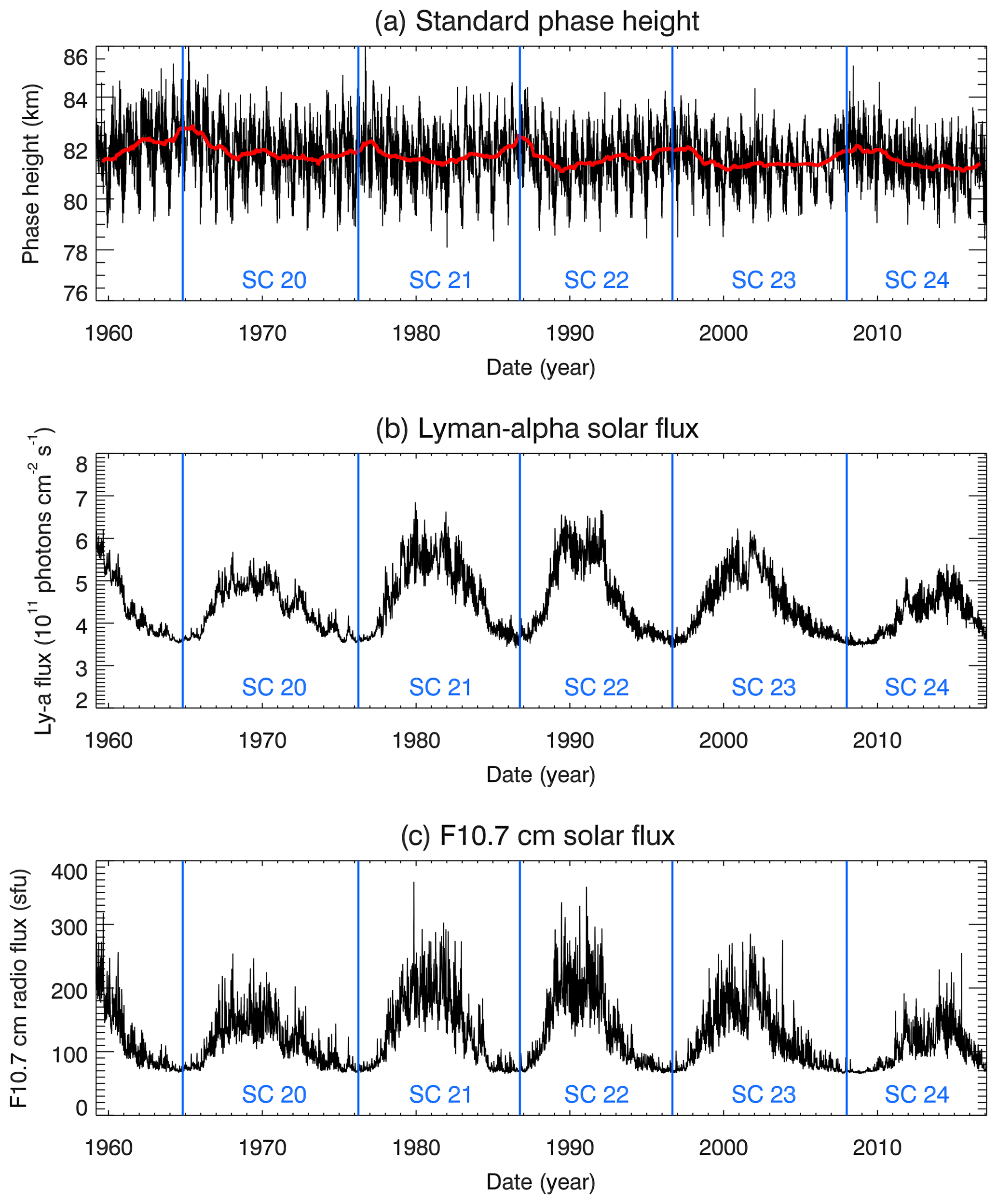
Figure 1Time series of standard phase height (a), solar Lyman-α (alpha) flux (b) and F10.7 cm solar flux (c) for the period from February 1959 to February 2017 (SC refers to solar cycle). The red line in the top panel corresponds to a 365-day running mean. The repeating pattern with a period of 1 year is the seasonal cycle in standard phase height data further discussed in Peters and Entzian (2015). An 11-year solar cycle signature is also discernible in the standard phase height time series.
3.1 Power spectral analysis
A classical approach is used to identify solar-driven 27-day variations in detrended daily time series. The solar proxy data sets employed here – i.e., Lyman-α flux and F10.7 cm flux data – were obtained from the LASP Interactive Solar IRradiance Datacenter (LISIRD). The Lyman-α data set is a composite of different observational data sets and a model based on F10.7 to cover the period between 1947 and the start of the observational data. In a first step, we apply a 41-day running mean and then calculate the anomaly as the deviation from the running mean for SPH and proxies of solar activity, like the Lyman-α and the F10.7 cm solar fluxes (see, e.g., Fig. 2). In a second step, a power spectral analysis of the anomaly time series based on wavelet analysis (Torrence and Compo, 1998) was carried out in order to determine spectra of the solar Lyman-α and the SPH time series (see Fig. 3). The calculation of the power spectrum uses the first 16 384 days only, due to the restriction of the wavelet analysis to time series whose number of data points corresponds to a power of 2. The solar Lyman-α spectrum shows a dominant band at a period of around 27 days, as expected, and an additional increase at about half that period (i.e., 13.5 days). Other proxies of solar variability have also been analyzed. The spectra of the F10.7 cm solar flux (SFL) and sunspot number (SPN) look similar (not shown). The SPH spectrum includes a much broader spectrum. Strong signatures at periods between 55 and 22 days are identified, which are weakly damped by the 41-day running mean. A white noise component below the 27-day variability is also found. This shows that the SPH spectrum is not the result of solar variability only – via photoionization by Lyman-α radiation – but includes other causes of variability, such as the atmospheric processes discussed later.
3.2 Superposed epoch analysis (SEA)
The analysis technique employed to extract solar-driven 27-day variations in standard phase height data is the superposed epoch analysis (further on referred to as SEA) technique (e.g., Howard, 1833; Chree, 1912), also known as composite analysis. The F10.7 cm solar radio flux or Lyman-α is used as a solar proxy in the current study. Figure 1b and c show Lyman-α and the F10.7 cm solar flux time series for the time period analyzed here, i.e., from February 1959 to February 2017.
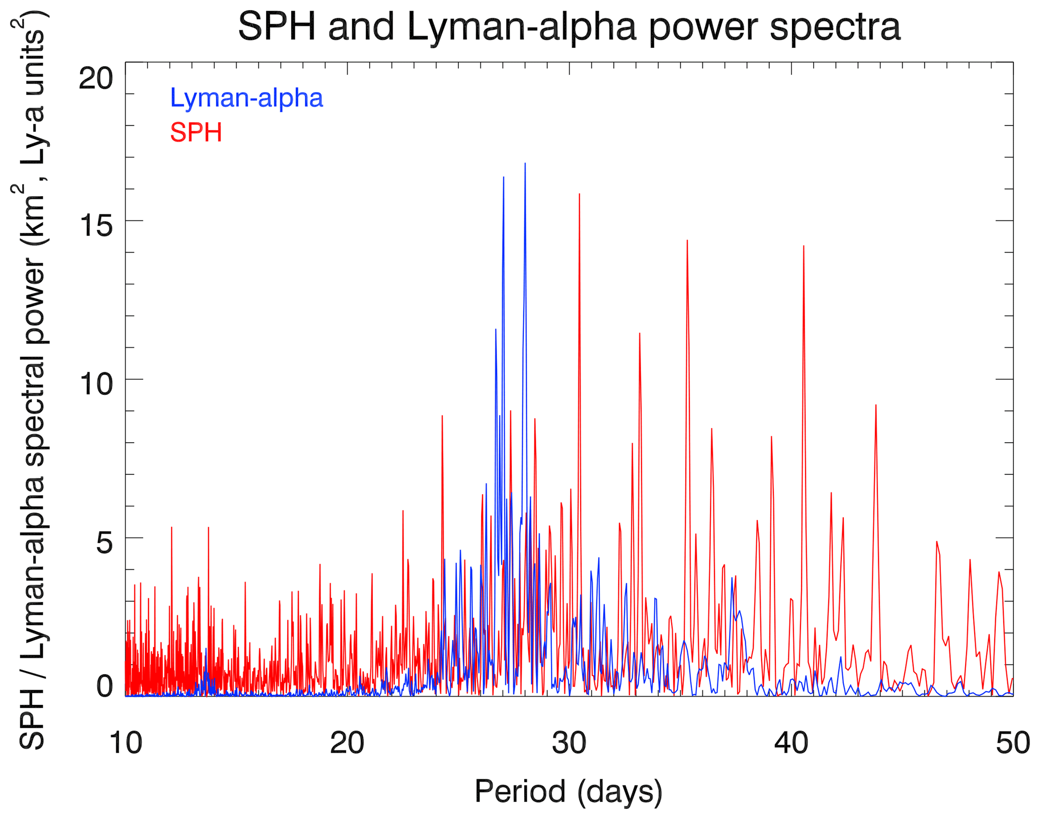
Figure 3Power spectra of the Lyman-α and the standard phase height (SPH) time series starting in February 1959.
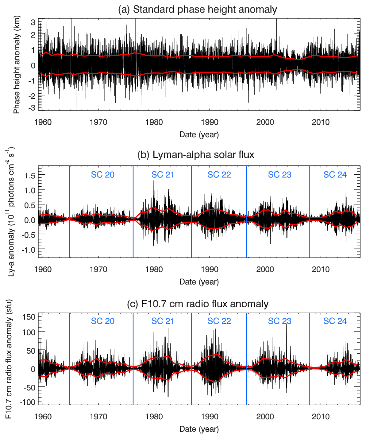
In a first step we determined anomaly time series by removing a 41-day running mean from the SPH, Lyman-α flux and F10.7 cm flux time series, covering the period from February 1959 to February 2017. Using 41 days is arbitrary to a certain extent, but the results are only weakly dependent on the width of the smoothing window used, as will be discussed in more detail in Sect. 4. Figure 2 shows the obtained anomaly time series for SPH (top panel), for Lyman-α solar flux (middle panel) and for the F10.7 cm solar flux (bottom panel). In order to quantify the variability of the anomalies as a function of time, we determined the standard deviation of the anomaly values in adjacent 100-day time bins. The red solid lines in the panels of Fig. 2 display the time variation of these standard deviations. The standard deviation of the SPH anomaly is on the order of several hundred meters, which is significantly larger than solar 27-day signature extracted below using the SEA.
Maxima in solar activity associated with the sun's differential rotation are identified automatically by searching for local maxima in the F10.7 cm flux time series smoothed with a 5-day running mean filter. This was done in the following way. We checked for every day of the time series whether the corresponding daily value is greater than or equal to the values in the period from −13 to +13 days around the corresponding day. If this is the case, a local maximum is identified. This way, multiple or minor maxima that are only a few days apart will not be identified. The identification of the maxima was checked visually, and the approach was found to work well (not shown).
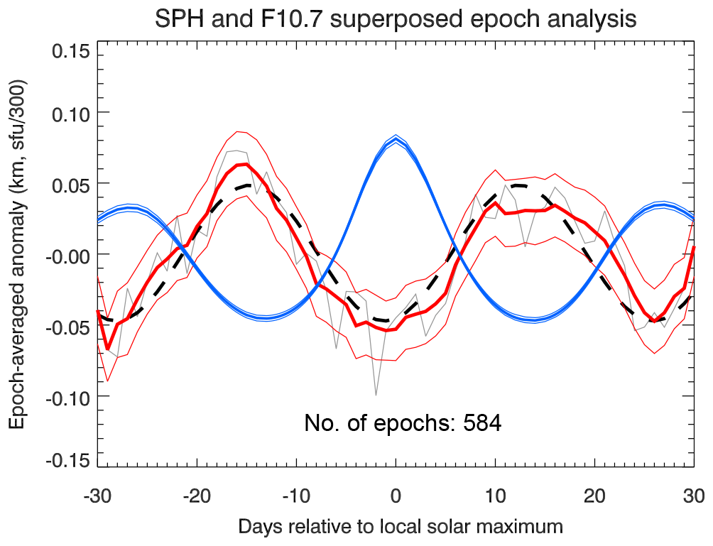
Figure 4Epoch-averaged standard phase height (SPH) and F10.7 cm solar flux anomalies for a total of 584 epochs. The thick blue line corresponds to the epoch-averaged F10.7 cm solar flux anomaly, and the thin blue lines show the standard errors of the mean for each day relative to local solar maximum. The grey thin line corresponds to the unsmoothed epoch-averaged SPH anomaly, also shown smoothed by a 5-day running mean in red. The thin red lines represent the standard error of the mean of epoch-averaged anomalies about the daily mean value and plotted around the smoothed anomaly to improve clarity. The black dashed line is a sinusoidal fit to the unsmoothed epoch-averaged standard phase height anomaly, with an amplitude of about 50 m.
The local solar maxima are the centers of the analyzed epochs, with each epoch covering 61 days, i.e., center date ±30 days. Then the standard phase height anomalies for every epoch are written to the rows of a N×61 matrix, N=584 being the number of epochs analyzed. The main step of the SEA consists of averaging the matrix column-wise, yielding the epoch-averaged standard phase height anomaly. Figure 4 shows the epoch-averaged F10.7 cm flux and the standard phase height anomalies for the entire data set from 1959 to 2017. The epoch-averaged F10.7 cm flux anomaly peaks at day 0 relative to local solar maximum, indicating that the epochs were selected correctly. The epoch-averaged standard phase height anomaly exhibits a periodic 27-day signature with an amplitude of about 50 m, and with a minimum occurring a few days before maximum solar activity. This finding is discussed below in Sect. 4, where we also investigate the dependence of the SEA results on solar activity (applying different F10.7 cm flux thresholds) and on season.
3.2.1 Significance testing
Periodic signatures in the epoch-averaged anomalies may also be introduced by effects entirely unrelated to changes in solar forcing. A single major anomaly in the time series, e.g., related to a major stratospheric warming, will only cancel out in the analysis if a sufficiently large number of epochs are available for analysis. Note that such an anomalous event may also lead to periodic variations in the epoch-averaged anomalies if overlapping epochs are used, i.e., if the major anomaly occurs after local solar maximum in one epoch and before local solar maximum in the following epoch. In other words, a repeating pattern in the epoch-averaged anomaly with a period of about 27 days is not necessarily an indication of the presence of a solar 27-day signature in the analyzed time series.
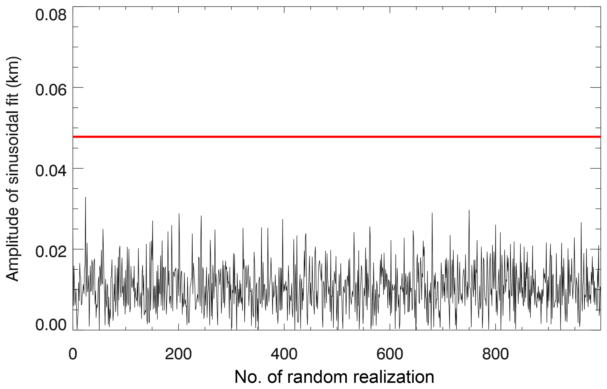
Figure 5Illustration of the Monte Carlo significance test. The red line shows the amplitude of a sinusoidal fit to the extracted 27-day signature in SPH. The black line shows the fitted amplitudes to epoch-averaged SPH anomalies for 1000 randomly chosen epoch ensembles. See text for more detailed information.
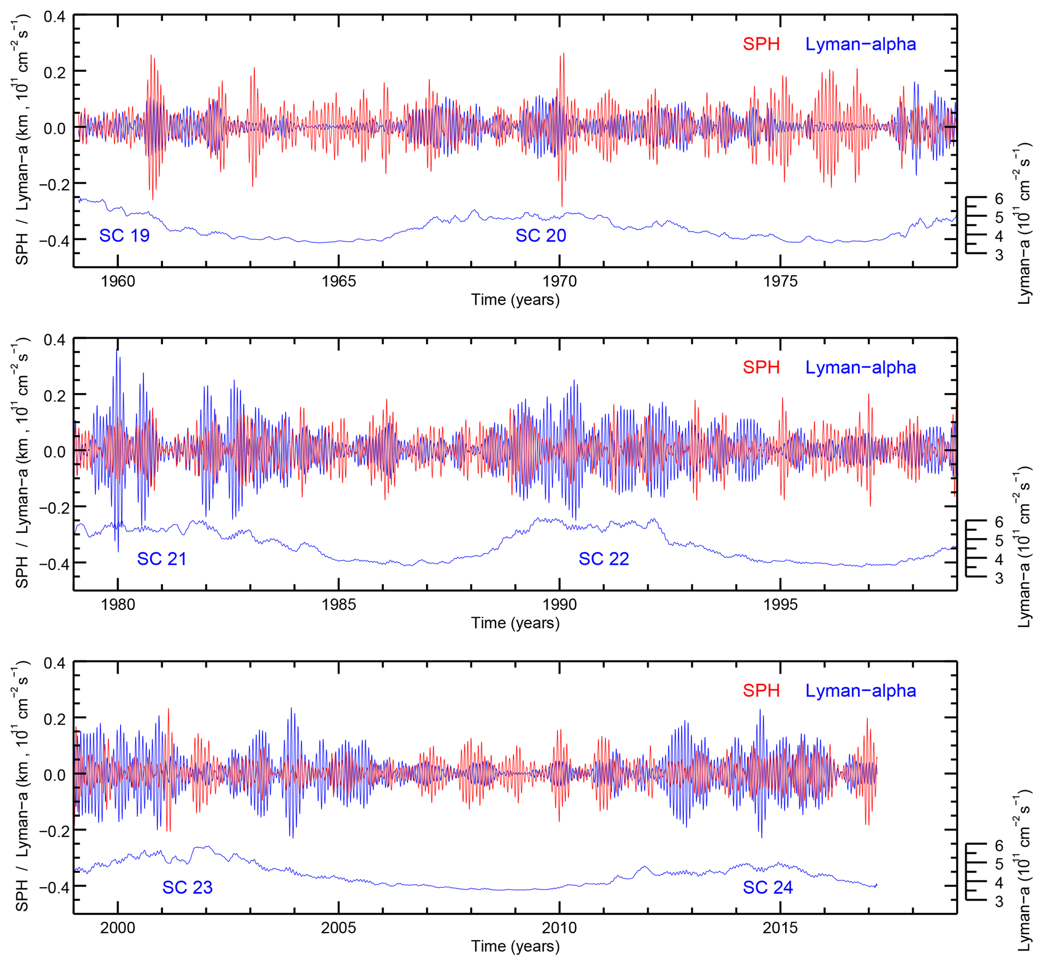
Figure 6Band-pass-filtered (24–31 days) Lyman-α (blue) and SPH (red) anomalies from February 1959 to February 2017 separated into three quasi-bidecadal intervals. The solar cycles (SC 19–SC 24) are also indicated by the smoothed 41-day running mean Lyman-α line (blue).
In order to test the significance of the obtained results, we applied the following Monte Carlo test. Rather than choosing the epochs centered at local solar maxima, the epochs are chosen randomly, using the same number of epochs as for the actual analysis. The SEA with randomly selected epochs is performed 1000 times, and a sinusoidal function is fitted to every single realization of the epoch-averaged standard phase height anomaly to determine its amplitude and phase. This is followed by checking for how many of the 1000 random cases the amplitude of the fitted sinusoidal function equals or exceeds the amplitude of the sinusoidal fit to the actual epoch-averaged standard phase height anomaly. Figure 5 shows as an example the amplitudes for the 1000 random realizations (in black) and the amplitude of the actual SEA (in red). The amplitude of the signature in the actual SEA is not reached by any of the random realizations, suggesting that the extracted 27-day signature in standard phase height is probably related to solar variability.
In Sect. 4.1 we apply the band-pass filtering method based on wavelet analysis after Torrence and Compo (1998) in order to identify for the selected anomaly time series a comparable variability as the studied solar-induced 27-day variation. The motivation comes from the result of the SEA (Fig. 4) that already showed that a 27-day signature is present in the SPH time series, which is strongly inversely correlated to the F10.7 cm solar flux or the Lyman-α flux. The used standard band-pass filter has a half width of about 10 % (∼3 days) of the fundamental period of 27 days; i.e., a band-pass filter of 24–31 days is applied. This filtered time series is also used for a cross-correlation analysis in Sect. 5. Furthermore, in Sect. 4.2 we apply the superposed epoch analysis using F10.7 cm solar flux data in order to investigate the identified 27-day signature (Fig. 4) in more detail. In Sect. 5 we apply a regression analysis to the standard phase height time series as well as ERA-Interim (Dee et al., 2011) and CMAM (McLandress et al., 2014) temperature and geopotential height time series to examine a possible link to atmospheric processes like planetary wave propagation and evolution.
4.1 Band-pass-filtered time series
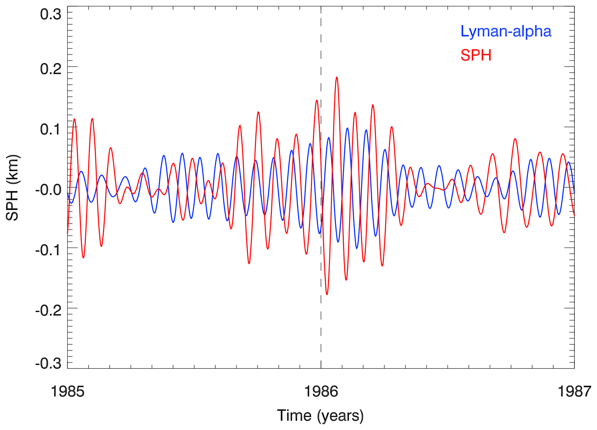
The band-pass-filtered (24–31 days) Lyman-α and SPH time series are shown in Fig. 6 for three separated quasi-bidecadal periods. In general, the Lyman-α time series shows a high variability with different fluctuations during solar maximum and solar minimum. During solar maximum the Lyman-α amplitudes are larger in solar cycles 21 and 22 than in solar cycle 20, for instance. Different seasonal SPH fluctuations are found for solar maximum in comparison to solar minimum. The SPH amplitudes are typically larger during winter compared to summer and for some solar cycles also appear to be larger during solar minimum than for solar maximum. Figure 7 shows as a typical example the winter 1985–1986 (note: with moderate Lyman-α amplitudes and larger SPH amplitudes). During May–July 1985 the two band-pass-filtered time series are out of phase (less obvious during May–July 1986) as expected from photoionization by Lyman-α, and the larger phase difference change during winter time may be due to atmospheric processes.
In addition to Fig. 7, the phase relationship is studied over the whole time series of 58 years. We examine the phasing between the SPH and Lyman-α, SFL and SPN anomaly series over all seasons. The results of a cross-correlation analysis (not shown) between those time series reveal a very weak inverse correlation between SPH and Lyman-α, SFL and SPN. Also in this case the SPH shows a negative lag of 1–3 days for all three cross-correlations, which means that on average the SPH minimum leads the maxima in solar activity proxies by a few days. This time lag is consistent with the time lag obtained from applying the superposed epoch analysis (see Sect. 4.2). Note that the cross-correlation was run over all seasons and all 58 years. This result supports the hypothesis that atmospheric processes determine the mean cross-correlation and finally the variability of SPH. In fact, in winter during solar minimum, when Lyman-α variability is rather small, it seems that atmospheric processes are dominant.
4.2 Superposed epoch analysis
The SEA results displayed in Fig. 4 already demonstrated that a 27-day signature is present in the SPH time series. The Monte Carlo significance test described above showed that the fitted amplitude of the epoch-averaged SPH anomalies did not reach the actual amplitude for any of the 1000 random ensembles, indicating that the 27-day signature in SPH in Fig. 4 is likely caused by the solar 27-day cycle. The 27-day signature in SPH has an amplitude of about 50 m and is thus significantly smaller than the overall SPH variability (see upper panel of Fig. 2).
The SEA was so far applied to the entire time series covering the period from February 1959 to February 2017, with a window width of 41 days when determining the anomaly time series. In the paragraphs below we investigate, how the SEA results depend on solar activity (applying different thresholds for the F10.7 cm flux), on season and on the width of the window. As will be seen, the sensitivity values are dependent on all of these assumptions.
The sensitivity parameter (or simply sensitivity) that quantifies the SPH dependence on solar activity is easily determined using the epoch-averaged F10.7 flux and SPH anomalies displayed in Fig. 4. The anomalies are plotted against each other in a scatter plot, and the sensitivity parameter is given by the slope of a linear regression line. Before the linear regression is performed, we determine the phase lag between solar maximum and SPH minimum using time-lagged cross-correlation. The SPH anomaly is then shifted by the corresponding time lag (4 days for the results displayed in Fig. 4), followed by the linear regression. For a smoothing window width of 41 days and considering all available epochs, a sensitivity of km (100 sfu)−1 is obtained.
We also determined the sensitivity of the SPH to the 11-year solar cycle. This is done by defining a regular F10.7 cm flux grid with a step size of 10 sfu, followed by averaging all daily F10.7 cm solar flux values – and the corresponding SPH values – for each 10 sfu bin. The resulting bin-averaged solar flux and SPH values are then plotted in a scatter plot, and the sensitivity is given by the slope of a line fitted by linear regression. The obtained value of the standard phase height sensitivity to solar forcing at the 11-year timescale is ) km (100 sfu)−1. This value agrees within combined uncertainties with the standard phase height sensitivity for the 27-day solar cycle of ) km (100 sfu)−1, which suggests similar driving mechanisms. This aspect will be discussed further in Sect. 6. We also note that the 11-year SPH sensitivity derived here is in good agreement with the value based on the results by Peters and Entzian (2015) of −0.387 km (100 sfu)−1. Peters and Entzian (2015) used the Lyman-α flux as a solar proxy so that a conversion to the F10.7 cm flux was required to convert their sensitivity value to units of km (100 sfu)−1. This was done using a linear fit to the Lyman-α flux as a function of F10.7 cm radio flux (see Fig. 8) for all available data between February 1959 and February 2017. Note that the correlation between the F10.7 cm radio flux and Lyman-α is weaker for solar minimum (e.g., Barth et al., 1990).
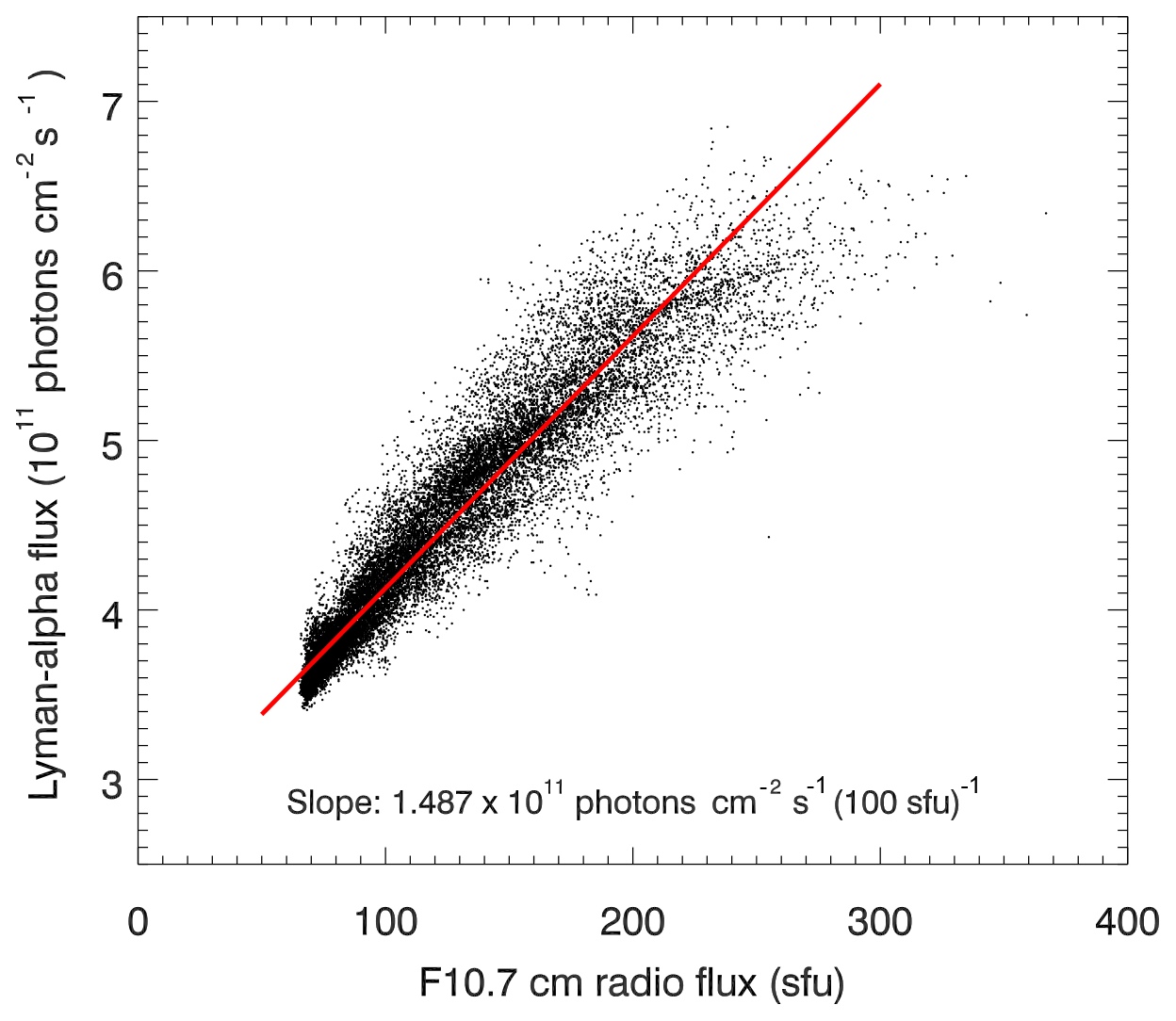
Figure 8Scatter plot of daily values of the Lyman-α flux and F10.7 cm radio flux for the period from February 1959 to February 2017. The red line corresponds to a linear regression of the data points.
Different tests were performed to study the dependence of the 27-day sensitivity of SPH on solar activity. First, we apply different solar activity thresholds (from 60 sfu up to 200 sfu in steps of 10 sfu) and only consider epochs for which the solar activity exceeds the assumed threshold on all days. The results of this test are listed in Table 1, and the dependence of the derived 27-day SPH sensitivity on solar activity is shown in Fig. 9. Table 1 lists the number of epochs available for the different solar activity thresholds, the temporal lag applied before performing the linear fit and the amplitude of the fitted sine as well as the results of the significance tests and the 27-day sensitivity value. The number of epochs decreases with an increasing solar activity threshold, as expected. For the lowest three solar activity thresholds, the significance test did not yield a single random ensemble with amplitudes exceeding the amplitude obtained in the actual analysis. The fraction generally increases with an increasing solar activity threshold and reaches about 35 % for a F10.7 cm flux threshold of 200 sfu. The time lag varies somewhat between −1 and −4, and the negative sign implies that the minimum in standard phase height precedes the maximum in solar activity. The reasons for this behavior are currently not well understood and will be discussed in Sect. 6.
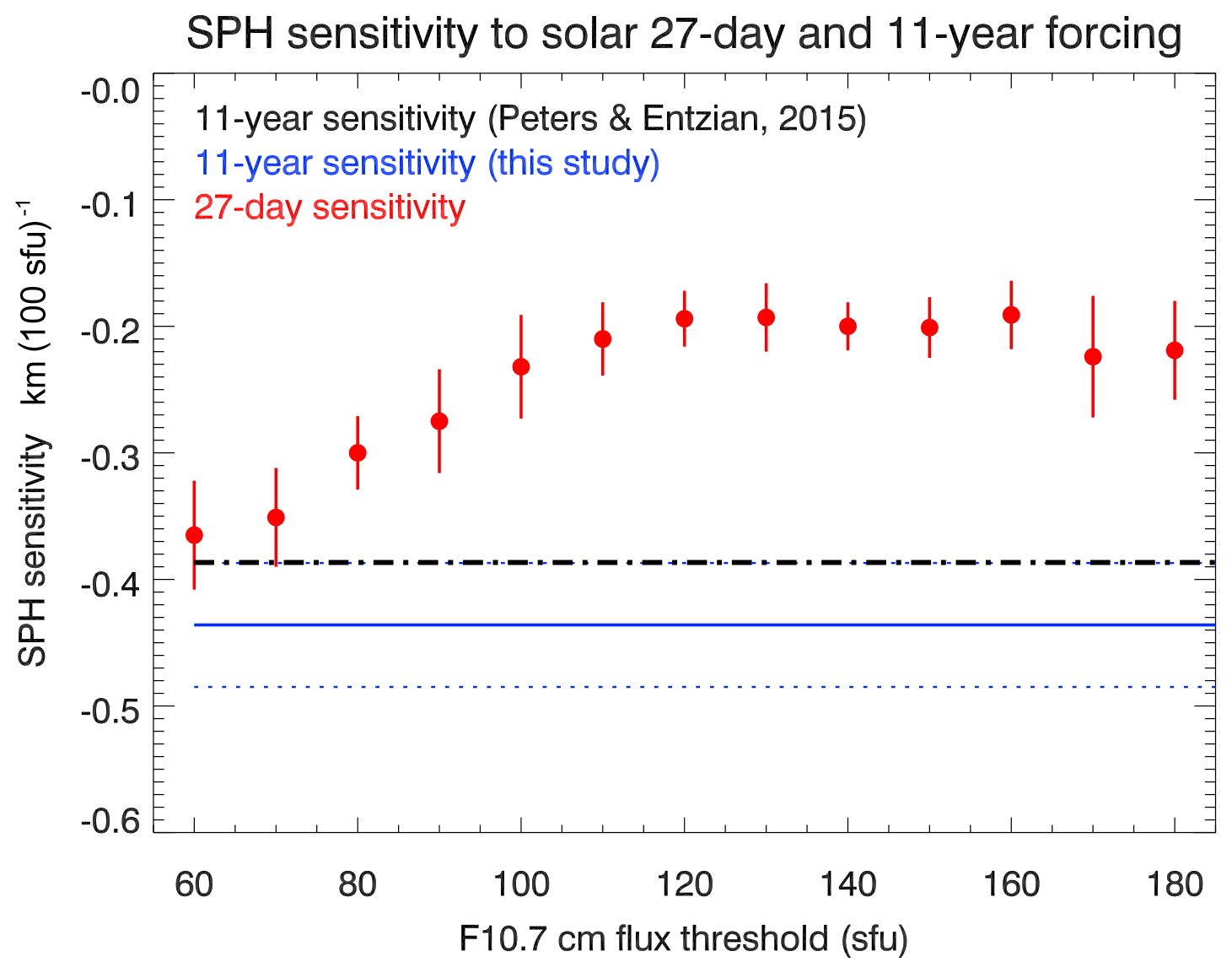
Figure 9SPH sensitivity to solar forcing for the 27-day and the 11-year solar cycle. The red circles show the 27-day sensitivity for different solar activity thresholds as described in the text. The blue line corresponds to the 11-year sensitivity determined in this study, and the dotted lines show the uncertainties. The black dash-dotted line displays the 11-year sensitivity determined by Peters and Entzian (2015).
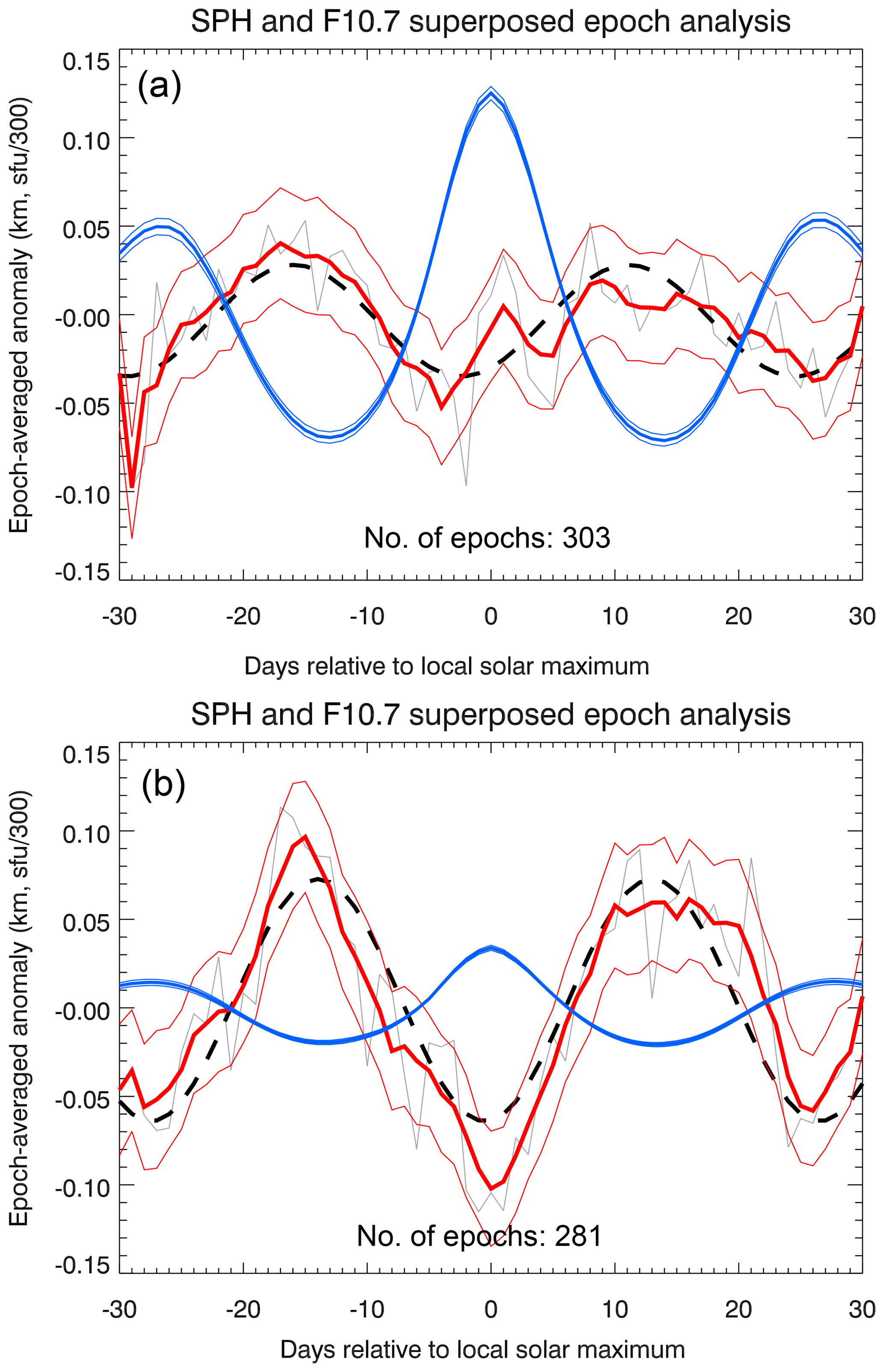
Figure 9 illustrates that the SPH sensitivity to solar forcing at the 27-day timescale depends on the solar activity threshold, but no simple or monotonous dependence is obvious. The figure also displays the SPH sensitivity to solar forcing for the 11-year solar cycle. The blue line shows the value determined in this study (including uncertainties shown as blue dotted lines), and the black dash-dotted line corresponds to the value determined in the study by Peters and Entzian (2015), based on the same SPH data set.
Table 1Overview of the results for different solar activity thresholds.
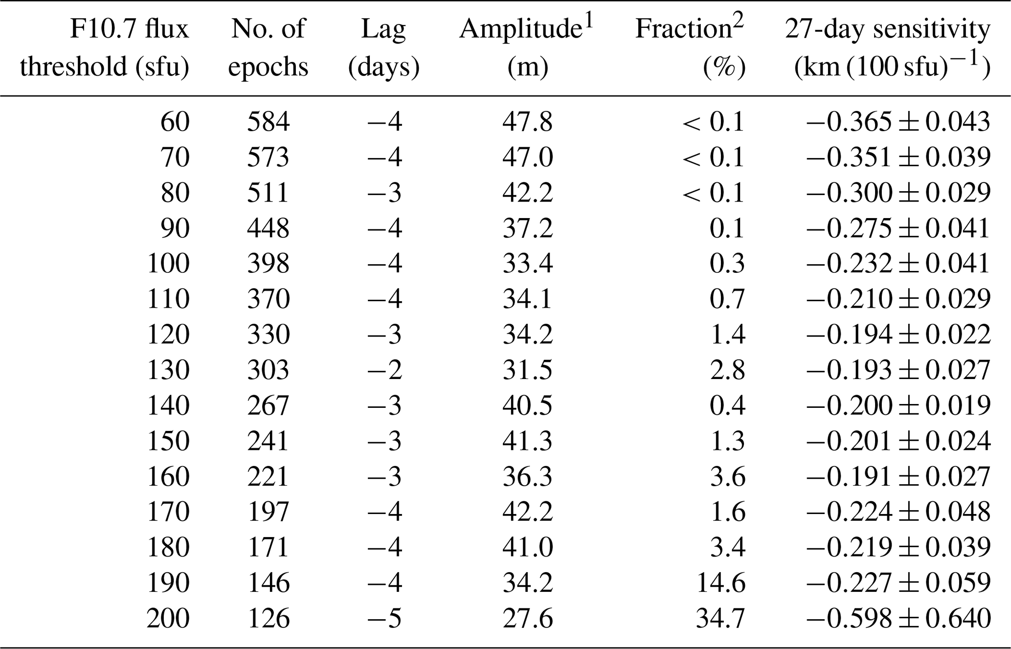
1 Amplitude of fitted sinusoidal function. 2 fraction of random realizations with amplitudes larger than actual data.
Next, we tested how the results differ between periods of low and enhanced solar activity. This was done by selecting epochs for which the F10.7 cm flux was either lower or greater than 130 sfu. The epoch-averaged SPH anomaly for F10.7 >130 sfu is shown in the upper panel of Fig. 10 and the one for F10.7 < 130 sfu in the bottom panel of this figure. Surprisingly, the amplitude of the extracted solar 27-day signature in SPH is larger for low solar activity than for higher solar activity. Because the absolute amplitude of the 27-day F10.7 cm flux variations for low solar activity is significantly smaller than during solar maximum, the SPH sensitivity to solar forcing at the 27-day scale and for low solar activity is, with a value of km (100 sfu)−1, also significantly larger than the value reported above.
We would like to point out that the phase lags listed in Table 1 are not inconsistent with the lower panel of Fig. 10. Table 1 shows the analysis results for epochs with solar activity exceeding a certain F10.7 cm flux threshold, while the lower panel of Fig. 10 shows the SEA results for epochs with solar activity lower than 130 sfu. The phase lag for low solar activity (bottom panel of Fig. 10) is smaller than for the other analyses. We currently do not have an explanation for this finding.
In addition, we investigated whether the solar 27-day signature in standard phase height depends on the season. For this purpose we consider “winter” to include the months October, November, December, January and February. “Summer” includes May, June, July, August and September. We use more than 3 months for each season in order to increase the number of epochs available for analysis. The smoothing window width is again 41, as above. The analysis results are listed in Table 2. The number of epochs used for the summer (243) and winter (244) seasons is almost identical, and the phase lag only differs by 1 day. However, the obtained amplitude is about a factor of 2 larger for the winter season than for summer. The SPH 27-day sensitivity for summer () km (100 sfu)−1) agrees within uncertainties with the all-year value ( km (100 sfu)−1), but for winter the value is () km (100 sfu)−1) slightly larger. The analysis for the summer months yields a relatively large fraction of random realizations with amplitudes larger than the actual analysis, which may contribute to the apparent differences. Potential reasons for this behavior are discussed below in Sect. 6.
Table 2Overview of the results for different seasons.
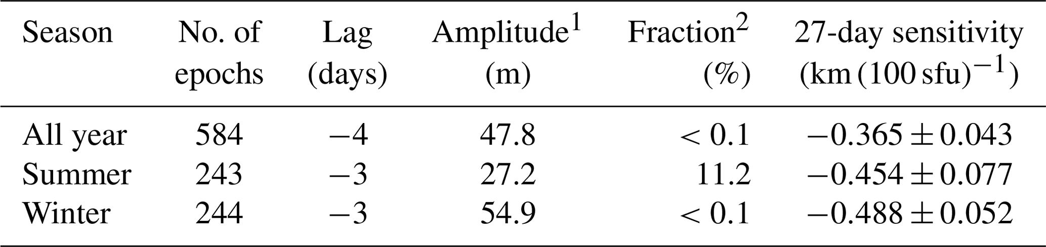
1 Amplitude of fitted sinusoidal function. 2 fraction of random realizations with amplitudes larger than actual data.
Next, we tested the effect of different smoothing windows – used to determine anomaly time series – on the results. The window width (w) was increased from 30 to 80 days in steps of 5 days. The obtained SPH sensitivities to solar forcing at the 27-day scale changed from km (100 sfu)−1 (w=30 days) to km (100 sfu)−1 (w=80 days). The dependence of the sensitivity on window width is not truly monotonous, but larger window widths have a tendency to be associated with larger absolute sensitivity values. Changing the window width by 10 days, leads to average changes in sensitivity of about 0.01 km (100 sfu)−1, corresponding to a relative change of about 3 %. We can therefore conclude that the obtained sensitivities are only weakly dependent on the smoothing window width.
In Sect. 5.1, we compare the variability of three data sets: the SPH time series, measured over the Eifel mountains (50∘ N, 6∘ E; western Germany) at about 82 km altitude (details are described in Sect. 2); the temperature profiles averaged over the Eifel mountain region (40–58∘ N, 0–12∘ E) from ERA-Interim data (Dee et al., 2011) and the Extended Canadian Middle Atmosphere Model (CMAM-Ext, CMAM30 results; McLandress et al., 2014). Model data were downloaded from the following web page: http://climate-modelling.canada.ca/climatemodeldata/cmam/cmam30/era_interim_adjustment/index.shtml (last access: 31 July 2018). Note that the CMAM-Ext model is nudged up to 1 hPa with ERA-Interim data; i.e., CMAM-Ext and ERA-Interim show a similar temporal evolution in the troposphere and stratosphere.
In addition, in Sect. 5.2 we apply a regression analysis between the SPH time series and the three-dimensional geopotential height (GH) field taken from CMAM, in order to examine the possible link between SPH evolution (band-pass filtered) and the hemispheric variability of the planetary wave field on a daily basis.
We also determined power spectra (not shown) of CMAM GH over the Eifel mountain region at pressure levels between 1 and 0.01 hPa, and significant spectral power for periods between 24 and 30 days was found, in agreement with the results presented by Schanz et al. (2016).
The CMAM data set used here also includes NO profiles. Unfortunately, the CMAM NO distribution in the mesosphere does not compare well with satellite observations with the Odin-SMR instrument (e.g., Kiviranta et al., 2018). This implies that an assessment of 27-day oscillations in CMAM NO data is problematic.
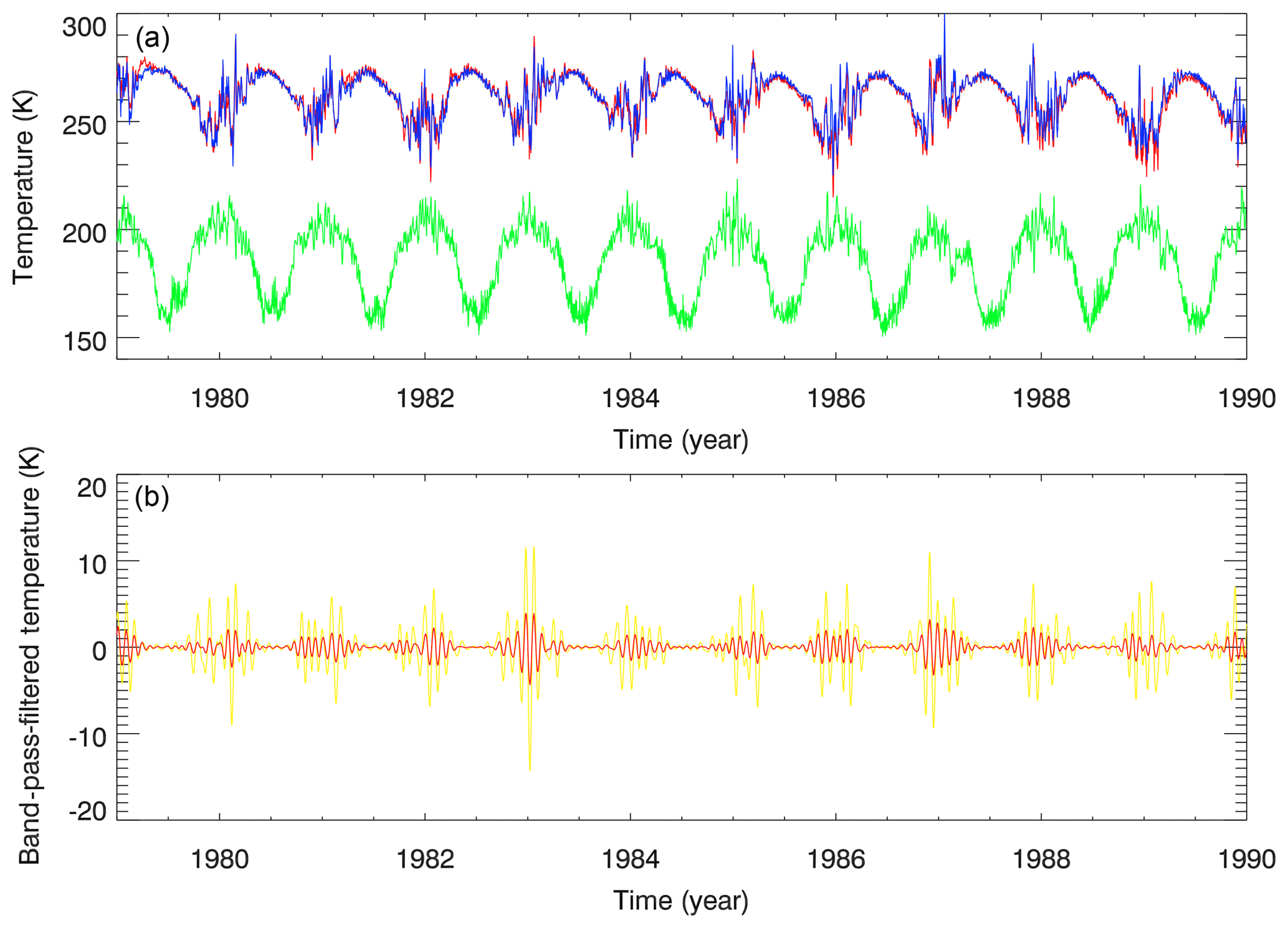
Figure 11(a) Temporal evolution of ERA-Interim (red) and CMAM (blue) temperatures at about 1 hPa (about 48 km) and CMAM temperature (green) at 0.01 hPa (about 80 km) averaged over the Eifel mountain region from 1 January 1979 to 31 December 1989. (b) Band-pass-filtered CMAM temperatures for a 24–31-day filter (red) and a 20–40-day filter (yellow) at 1 hPa.
5.1 Comparison of time series over Eifel mountains
The ERA-Interim (red) and CMAM (blue) temperature evolutions at about 1 hPa over the Eifel mountain region are in good agreement, as shown in the upper panel of Fig. 11. This is expected because of the nudging procedure used in CMAM. This is demonstrated as an example for the decade from 1979 to 1989. A stratopause warming is found in each summer season and a highly disturbed winter evolution, mainly due to the action of planetary waves. Results of a band-pass filter analysis are shown in the lower panel of Fig. 11 indicating large amplitudes of about 1–5 K for a 24–31-day filter during winter and up to 10 K in the broader 20–40-day filter band. Both filter bands are in phase but show different amplitudes for different boreal winters. That means that especially in winter a high variability in the stratopause temperature occurs with a dominant signal in the 24–31-day filter band, which refers to the enhanced ultra-long planetary wave activity.
The top panel of Fig. 11 shows the CMAM temperature evolution at 0.01 hPa in green. The lowest temperatures at this upper mesospheric level are found in summer – as known, e.g., from OH* rotational temperature measurements at Wuppertal (51∘ N, 7∘ E; Kalicinsky et al., 2016) – with an inverse correlation to stratopause temperature. In each winter we also found a strong inverse correlation in the temperature variability between both layers induced by planetary wave activity which also appears in other meteorological fields due to the quasi-geostrophic balance. This ultra-long wave activity extends into the mesosphere as known from to the vertical propagation of ultra-long planetary waves (Charney and Drazin, 1961) in an eastward-directed background flow, including vacillation cycle behavior as shown by Holton and Mass (1976). The hemispheric structure of ultra-long wave oscillations in the 24–31-day filter band is investigated in the next subsection.
5.2 Regression of standard phase heights and CMAM geopotential heights
Following classical textbooks (e.g., Taubenheim, 1969) the regression between two time series is defined by the correlation between both multiplied by the standard deviation of the first series and divided by the standard deviation of the second series. A time lag (lead) is introduced by a negative (positive) shift of days for the first time series, followed by repeated calculation. As the second time series we choose the 24–31-day band-pass-filtered SPH, and as the first time series we use the nonfiltered GH anomaly available at 64 longitudes (covering the range from 0 to 360∘ in steps of 5.625∘) and at 17 latitudes (between 0 and 85.76∘ N in steps of about 5∘) and at each model pressure layer from the surface up to 0.001 hPa (62 layers). Selected results of the regression coefficient calculation are shown in Fig. 12 for lags of −12 and 0 days in order to examine the periodic behavior. The results are presented for 0.01 hPa (about 80 km in the upper mesosphere, about the layer of SPH measurements; panels a and b) and for 1 hPa (about 48 km; panels c and d) near the stratopause. All plots show extended regions of positive and of negative regression coefficients, indicating large-scale structures of similar regression as expected from the action of ultra-long planetary waves (about wave 1 to 3). In the upper mesosphere (0.01 hPa) and for a lag of −12 days (Fig. 12a), we found a positive GH anomaly of 300 m for 1 km SPH change over central Europe.
For a 0-day lag (Fig. 12b) – i.e., about half a 27-day solar period later – a negative regression was found in a similar order. That means that over central Europe, a GH change 12 days before is positively correlated with band-pass-filtered SPH variability. Twelve days later there is a negative correlation. The hemispheric patterns are comparable, indicating an ultra-long wave structure. Note that we also determined the regression between SPH and CMAM GH for a lag of −15 days (not shown), and the results are very similar to the results for a lag of −12 days.
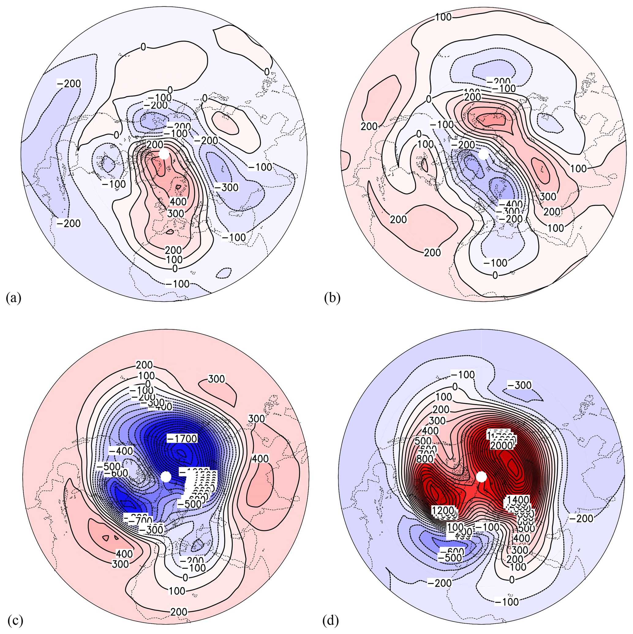
Figure 12Regression (in m km−1) between the SPH (24–31-day filtered) time series and the CMAM geopotential height time series at 0.01 hPa (a, b) and at 1 hPa (c, d) for time lags of −12 days (a, c) and 0 days (b, d) for the period October 1985 to April 1986. The contour interval is 100 m km−1, and reddish (bluish) areas show positive (negative) regression coefficients.
At 1 hPa and for a lag of −12 days (Fig. 12c), we found a positive GH anomaly of 500 m for 1 km SPH change over the central North Atlantic. For 0-day lag (Fig. 12d) – i.e., half a 27-day solar cycle later – a negative regression was found in a similar order. That means that over the central North Atlantic, a GH change 12 days before is positively correlated with band-pass-filtered SPH variability at 80 km altitude. Twelve days later the correlation is negative. In the stratopause region (Fig. 12c and d) the planetary wave regression patterns are more intense, showing statistically significant correlations.
In the upper mesosphere, the negative regression pattern between the GH anomaly and the 24–31-day band-pass-filtered SPH time series over central Europe at about 80 km altitude for a lag of 0 days may be explained by horizontal planetary wave transport. An increase (decrease) of NO density is caused by southward (northward) transport of NO by ultra-long waves for an observed mean positive latitudinal NO gradient in a region between a high and low (low and high) pressure system. Vertical transport of NO by lifting or subsidence is assumed to be weak, as is diffusion. The consequence is an increase (decrease) of the free electron number density due to photoionization as discussed by von Cossart and Entzian (1976), with a lower (higher) SPH. That implies that SPH shows a negative (positive) regression with the GH anomaly on the easterly (westerly) side of the high-pressure center.
This hypothesis has to be examined further in an atmospheric general circulation model including a chemistry and ion model, which is beyond the diagnostic study presented here.
The positive correlation pattern for a lag of −12 days (Fig. 12a) follows from the quasiperiodic 27-day oscillation behavior of the ultra-long wave structure. In the stratopause layer the regression pattern is positively (negatively) correlated to the 24–31-day band-pass-filtered SPH time series over the polar region for a lag of 0 days (−12 days) – see Fig. 12c and d – indicating a polar vortex weakening (strengthening). The vortex weakening is linked with an intrusion of subtropical air into the polar region over the North Atlantic, as known from some major stratospheric warming events in wintertime (e.g., Peters et al., 2014; Harvey et al., 2018). A dominant wave 1 pattern occurs with a strong wave 2. In general the results reveal an atmospheric influence especially of ultra-long planetary waves on the 24–31-day band-pass-filtered SPH time series during wintertime and solar minimum.
In this study we investigated variability in SPH at temporal scales close to the solar 27-day cycle. Different analysis techniques – i.e., cross-correlation analysis and superposed epoch analysis – were applied to extract a potential solar-driven 27-day signature in SPH data covering almost six solar cycles.
The SEA, when applied to the entire SPH data set, yields evidence for a clear periodic 27-day signature with an amplitude of about 50 m, which is likely caused by the solar 27-day cycle, as demonstrated by a Monte Carlo significance analysis. An independent piece of evidence indicating that the identified 27-day signature in SPH is caused by solar forcing is the finding that the determined SPH sensitivity to solar variability at the 27-day scale is in good agreement with the sensitivity for the 11-year solar cycle. SPH is more or less inversely correlated to solar forcing, which is consistent with the simple picture that enhanced photoionization of NO leads to an increase in free electron density and subsequently to a decrease in SPH. However, several of our findings cannot be reconciled with a purely photochemical mechanism.
First, both the SEA and the cross-correlation analysis consistently show that the minimum in SPH precedes the maximum in solar forcing by a few days, indicating the action of other forcings or atmospheric effects. Note that negative phase lags are also found in the response of upper stratospheric ozone to the solar 27-day forcing, which can be explained by a feedback of the solar 27-day signature in temperature on ozone (e.g., Brasseur et al., 1987; Keating et al., 1987). This specific example is not directly relevant for the results presented here, but demonstrates that negative phase lags can in principle occur.
Second, not only is the SPH sensitivity to solar forcing larger for periods of low solar activity, but even the amplitude of the potential solar 27-day signature is larger during solar minimum, which is currently not understood at all. Interestingly, Gruzdev et al. (2009) found in their HAMMONIA model studies a generally nonlinear atmospheric response to solar forcing, with sensitivities increasing with decreasing forcing. This is, in part, consistent with our results. However, Gruzdev et al. (2009) emphasized that the amplitude of the atmospheric response does not increase with decreasing forcing, which is inconsistent with our results on the SPH response to solar forcing. The apparent increase in the amplitude of the potential 27-day signature in SPH with decreasing solar activity may also be an artifact and caused by effects unrelated to solar variations. If this is the case, it is, however, unexpected that the phase relationship between solar forcing and the potential response in SPH essentially remains the same, independent of solar activity. This could be a synchronization effect. In this context it is important to mention that Ebel et al. (1981) performed a cross-spectral analysis of the solar F10.7 cm flux and planetary wave activity in the stratosphere at pressure levels between 10 and 50 hPa. They found significant correlations between solar variability and the amplitude of planetary waves.
Third, the amplitude of the potential solar 27-day signature in SPH is about a factor of 2 larger during winter than during summer. It is well known that, due to the winter anomaly, the SPH amplitudes are increased in winter by larger downward transport of NO from the thermosphere and subsequent photoionization (e.g., Peters et al., 2017; Garcia et al., 1987). Garcia et al. (1987) examined the electron density anomalies in the boreal D region in a coupled model with neutral and ion photochemistry as well as transport by planetary waves. They found that anomalies can be understood in terms of auroral production of nitric oxide in the polar night and its subsequent transport and ionization. In particular, their results indicate the importance of horizonal ultra-long planetary wave transport for many of the observed features. In addition, Hendricks et al. (2015) clearly demonstrated the impact of the 27-day solar cycle on NO production in the auroral zone in satellite measurements during events of energetic particle precipitation (EPP). The authors found larger amplitudes of the EPP-driven 27-day signatures in NO during winter than during summer, which may contribute to the larger amplitudes of the 27-day signatures in SPH reported here. Gruzdev et al. (2009) also discussed seasonal variations of the atmospheric response to the solar 27-day cycle. For extratropical latitudes they report that the sensitivities are for many parameters larger in winter than in summer.
In this context it is also important to mention that Pancheva et al. (1991) investigated quasi 27-day fluctuations in ground-based measurements of radio wave absorption in the lower ionosphere. They found indications for several aspects that are in good qualitative agreement with the results presented here. The reported absorption fluctuations are largest during winter near solar minimum, suggesting a dynamical forcing, which may be of solar origin, as the authors suggest.
In order to investigate the influence of planetary waves, temperature data taken from the ERA-Interim reanalysis as well as from model simulations with a nudged version of CMAM were used in the current study. The presented results provide clear evidence that planetary waves are associated with spectral power in the quasi 27-day period range and lead to corresponding variations in SPH. In the upper mesosphere, the negative regression pattern between the GH anomaly and the 24–31-day band-pass-filtered SPH time series over central Europe for a lag of 0 days may be explained by an increase of NO density caused by southward transport of NO by ultra-long waves in an observed mean positive latitudinal NO gradient, in a region between high and low pressure. In this context it should be mentioned that Siskind et al. (1997) discussed the role of planetary wave mixing on the latitudinal NO gradient in the winter time mesosphere.
The different analysis techniques provide complementary approaches to investigate different sources of variability in SPH. While the SEA allows a robust identification of a solar-driven 27-day signature, the regression analysis applied to SPH and CMAM GH allows separating dynamical effects. The presented investigations allowed improving the scientific understanding of several aspects of solar and dynamical influences on SPH. However, an overall and coherent picture is still missing, as several of the reported effects are difficult to quantify and understand. In addition, a potential impact of solar variability on planetary wave activity is not well understood.
In the context of 27-day variations in SPH, it is also relevant that a solar 27-day signature in noctilucent cloud (NLC) altitude was recently discovered (Thurairajah et al., 2017; Köhnke et al., 2018). The signature has an amplitude of about 100–200 m. Köhnke et al. (2018) provide a qualitative explanation for phase relationship of the identified 27-day signature in NLC altitude, NLC occurrence rate and temperature at the polar summer mesopause. The 27-day signature in NLC parameters is likely mainly driven by dynamical effects (see Köhnke et al., 2018). The main reason is that the phase relationship between the 27-day signatures in temperature and H2O mixing ratio at the summer mesopause found by Thomas et al. (2015) is inconsistent with a purely photochemical process, but easily explained by a solar modulation of the upwelling in the polar summer mesosphere.
Further insight into the underlying processes may be gained by dedicated model simulations using a general circulation model, coupled with an ion chemical module capable of modeling all relevant physical (particularly dynamical) and chemical processes.
We identified a solar-driven 27-day signature in standard phase height (SPH) measurements. Employing a Monte Carlo approach, the 27-day solar cycle signature was shown to be highly significant. SPH is inversely correlated to the solar forcing (at the 27-day scale), but the phase height minimum occurs a few days before the solar maximum, indicating that the 27-day solar cycle signature in standard phase heights is not only a consequence of variable photoionization of NO. We argue that nontrivial dynamical effects potentially cause the observed phase lags. The exact mechanisms are, however, currently unknown. It was demonstrated that both the sensitivity of standard phase heights to solar forcing at the 27-day scale as well as the amplitude of the 27-day signature depend on several parameters, including solar activity, season and the specific prior treatment of the time series. If the entire time series is analyzed, the 27-day signature in standard phase height has an amplitude of about 50 m and a 27-day sensitivity value is obtained that agrees within combined uncertainties with the sensitivity value of the 11-year solar cycle (i.e., km (100 sfu)−1). The latter value is in agreement with the study by Peters and Entzian (2015). To our knowledge, we demonstrated for the first time the possible link between band-pass-filtered (24–30 days) SPH time series and large-scale geopotential height fields in the extratropical boreal upper stratosphere and mesosphere during solar minimum. We identified a planetary wave-1 and wave-2 structure in the regression coefficient distribution in the upper stratosphere and mesosphere showing an oscillation pattern with a period of about 27 days. Several findings are unexpected and currently not fully understood. A full understanding of these effects requires dedicated model simulations considering all relevant physical and chemical processes.
The standard phase height data are available upon request from peters@iap-kborn.de. The Lyman-α and F10.7 solar flux time series are accessible through the LISIRD web portal (http://lasp.colorado.edu/lisird/, last access: 31 July 2018). CMAM model data are available from the following web page: http://climate-modelling.canada.ca/climatemodeldata/ (last access: 31 July 2018). The ERA-Interim data can be downloaded from https://apps.ecmwf.int/datasets/ (last access: 31 July 2018).
DHWP and GE carried out the retrieval of standard phase height data from the radio signal received in Kühlungsborn. CvS performed the superposed epoch analysis and wrote the main part of the paper. DHWP carried out the spectral analysis and the comparison of standard phase height data with ERA-I and CMAM data. DHWP and GE contributed parts of the text. All authors discussed the content of the paper and proofread it.
The authors declare that they have no conflict of interest.
This article is part of the special issue “Layered phenomena in the mesopause region (ACP/AMT inter-journal SI)”. It is a result of the LPMR workshop 2017 (LPMR-2017), Kühlungsborn, Germany, 18–22 September 2017.
The authors are indebted to the Leibniz-Institute of Atmospheric Physics in
Kühlungsborn and the precursor institutions for running the phase height
measurements over more than 5 decades. We are grateful to the many
technicians who were involved in maintaining the recordings. We thank
Brigitte Wecke for plotting Fig. 12 and Jorge Chau for carefully reading the
manuscript and making suggestions for improvements. We wish to thank
Deutscher Wetterdienst, ECMWF, the Royal Observatory of Belgium (SILSO, 2017;
SIDC, version 2) and LISIRD (http://lasp.colorado.edu/lisird/, last
access: 31 July 2018) of Colorado University (USA) for providing reanalysis
data, the solar Lyman-α time series and F10.7 cm time series,
respectively. This work was supported by the University of Greifswald and by
the German Federal Ministry of Education and Research (BMBF) through ROMIC
(Role Of the Middle atmosphere In Climate) project OHcycle (grant 01LG1215A).
We acknowledge support for the article processing charges from the DFG
(German Research Foundation, 393148499) and the Open Access Publication Fund
of the University of Greifswald.
Edited by:
Martin Dameris
Reviewed by: three anonymous referees
Barth, C. A., Tobiska, W. K., Rottman, G. J., and White, O. R.: Comparison of 10.7 cm radio flux with SME solar Lyman alpha flux, Geophys. Res. Lett., 17, 571–574, 1990. a
Brasseur, G., DeRudder, A., Keating, G. M., and Pitts, M. C.: Response of middle atmosphere to short-term solar ultraviolet variations, 2, Theory, J. Geophys. Res., 92, 903–914, https://doi.org/10.1029/JD092iD01p00903, 1987. a
Charney, J. G. and Drazin, P. G.: Propagation of planetary-scale disturbances from the lower into the upper atmosphere, J. Geophys. Res., 66, 83–109, https://doi.org/10.1029/JZ066i001p00083, 1961. a
Chree, C.: Some phenomena of sunspots and of terrestrial magnetism at Kew Observatory, Philos. Trans. R. Soc. London A, 212, 75–116, https://doi.org/10.1098/rsta.1913.0003, 1912. a
Dee, D. P., Uppala, S. M., Simmons, A. J., Berrisford, P., Poli, P., Kobayashi, S., Andrae, U., Balmaseda, M. A., Balsamo, G., Bauer, P., Bechtold, P., Beljaars, A. C. M., van de Berg, I., Biblot, J., Bormann, N., Delsol, C., Dragani, R., Fuentes, M., Greer, A. J., Haimberger, L., Healy, S. B., Hersbach, H., Holm, E. V., Isaksen, L., Kallberg, P., Kohler, M., Matricardi, M., McNally, A. P., Mong-Sanz, B. M., Morcette, J.-J., Park, B.-K., Peubey, C., de Rosnay, P., Tavolato, C., Thepaut, J. N., and Vitart, F.: The ERA-Interim reanalysis: Configuration and performance of the data assimilation system, Q. J. Roy. Meteorol. Soc., 137, 553–597, https://doi.org/10.1002/qj.828, 2011. a, b
Ebel, A., Schwister, B., and Labitzke, K.: Planetary waves and solar activity in the stratosphere between 50 and 10 mbar, J. Geophys. Res., 86, 9729–9738, https://doi.org/10.1029/JC086iC10p09729, 1981. a, b
Fytterer, T., Santee, M. L., Sinnhuber, M., and Wang, S.: The 27 day solar rotational effect on mesospheric nighttime OH and O3 observations induced by geomagnetic activity, J. Geophys. Res.-Space, 120, 7926–7936, https://doi.org/10.1002/2015JA021183, 2015. a
Garcia, R. R., Solomon, S., Avery, S. K., and Reid, G. C.: Transport of nitric oxide and the D-region winter anomaly, J. Geophys. Res. 92, 977–994, 1987. a, b
Gruzdev, A. N., Schmidt, H., and Brasseur, G. P.: The effect of the solar rotational irradiance variation on the middle and upper atmosphere calculated by a three-dimensional chemistry-climate model, Atmos. Chem. Phys., 9, 595–614, https://doi.org/10.5194/acp-9-595-2009, 2009. a, b, c
Hale, G. E., Ellerman, F., Nicholson, S. B., and Joy, A. H.: The Magnetic Polarity of Sun-Spots, Astrophys. J., 49, p. 153, https://doi.org/10.1086/142452, 1919. a
Harvey, V. L., Randall, C. E., Goncharenko, L., Becker, E., and France, J.: On the upward extension of the polar vortices into the mesosphere, J. Geophys. Res.-Atmos., 123, 9171–9191, https://doi.org/10.1029/2018JD028815, 2018. a
Hendrickx, K., Megner, L., Gumbel, J., Siskind, D. E., Orsolini, Y. J., Nesse Tyssøy, N., and Hervig, M.: Observation of 27 day solar cycles in the production and mesospheric descent of EPP-produced NO, J. Geophys. Res., 120, 10, 8978–8988, https://doi.org/10.1002/2015JA021441, 2015. a
Hong, P. K., Miyahara, H., Yokoyama, Y., Takahashi, Y., and Sato, M.: Implications for the low latitude cloud formations from solar activity and the quasi-biennial oscillation, J. Atmos. Sol.-Terr. Phys., 73, 587–593, https://doi.org/10.1016/j.jastp.2010.11.026, 2011. a
Hood, L. L.: Coupled Stratospheric Ozone and Temperature Responses to Short-Term Changes in Solar Ultraviolet Flux: An Analysis of Nimbus 7 SBUV and SAMS data, J. Geophys. Res., 91, 5264–5276, https://doi.org/10.1029/JD091iD04p05264, 1986. a, b
Hood, L. L.: Lagged response of tropical tropospheric temperature to solar ultraviolet variations on intraseasonal time scales, Geophys. Res. Lett., 32, 4066–4075, https://doi.org/10.1002/2016GL068855, 2016. a
Holton, J. R. and Mass, C.: Stratospheric vacillation cycles, J. Atmos. Sci., 33, 2218–2225, 1976. a
Howard, L.: The climate of London, 2nd edn., London, 1833. a
Huang, K. M., Liu, A. Z., Zhang, S. D., Yi, F., Huang, C. M., Gan, Q., Gong, Y., Zhang, Y. H., and Wang, R.: Observational evidence of quasi-27-day oscillation propagating from the lower atmosphere to the mesosphere over 20∘ N, Ann. Geophys., 33, 1321–1330, https://doi.org/10.5194/angeo-33-1321-2015, 2015.
Kalicinsky, C., Knieling, P., Koppmann, R., Offermann, D., Steinbrecht, W., and Wintel, J.: Long-term dynamics of OH* temperatures over central Europe: trends and solar correlations, Atmos. Chem. Phys., 16, 15033–15047, https://doi.org/10.5194/acp-16-15033-2016, 2016. a
Kalicinsky, C., Peters, D. H. W., Entzian, G., Knieling, P., and Matthias, V.: Observational evidence for a quasi-bidecadal oscillation in the summer mesopause region over Western Europe, J. Atmos. Sol.-Terr. Phys., 178, 7–16, https://doi.org/10.1016/j.jastp.2018.05.008, 2018. a
Keating, G. M., Pitts, M. C., Brasseur, G., and De Rudder, A.: Response of middle atmosphere to short-term solar ultraviolet variations: 1. Observations, J. Geophys. Res., 92, 889–902, https://doi.org/10.1029/JD092iD01p00889, 1987. a
Kiviranta, J., Pérot, K., Eriksson, P., and Murtagh, D.: An empirical model of nitric oxide in the upper mesosphere and lower thermosphere based on 12 years of Odin SMR measurements, Atmos. Chem. Phys., 18, 13393–13410, https://doi.org/10.5194/acp-18-13393-2018, 2018. a
Köhnke, M., von Savigny, C., and Robert, C.: Observation of a 27-day solar signature in noctilucent cloud altitude, Adv. Space Res., 61, 2531–2539, https://doi.org/10.1016/j.asr.2018.02.035, 2018. a, b, c, d
Lednytskyy, O., von Savigny, C., and Weber, M.: Sensitivity of equatorial atomic oxygen in the MLT region to the 11-year and 27-day solar cycle, J. Atmos. Sol.-Terr. Phys., 162, 136–150, https://doi.org/10.1016/j.jastp.2016.11.003, 2017. a
McLandress, C., Plummer, D. A., and Shepherd, T. G.: Technical Note: A simple procedure for removing temporal discontinuities in ERA-Interim upper stratospheric temperatures for use in nudged chemistry-climate model simulations, Atmos. Chem. Phys., 14, 1547–1555, https://doi.org/10.5194/acp-14-1547-2014, 2014. a, b
Meraner, K. and Schmidt, H.: Transport of Nitrogen Oxides through the winter mesopause in HAMMONIA, J. Geophys. Res.-Atmos., 121, 2556–2570, 2016.
Pancheva, D., Schminder, R., and Lastovicka, J.: 27-day fluctuations in the ionospheric D-region, J. Atmos. Terr. Phys., 53, 1145–1150, https://doi.org/10.1016/0021-9169(91)90064-E, 1991. a
Peters, D. H. W., Hallgren, K., Lübken, F.-J., and Hartogh, P.: Subseasonal variability of water vapor in the upper stratosphere/lower mesosphere over Northern Europe in winter 2009/2010, J. Atmos. Sol.-Terr. Phys., 114, 9–18, https://doi.org/10.1016/j.jastp.2014.03.007, 2014. a
Peters, D. H. W. and Entzian, G.: Long-term variability of 50 years of standard phase-height measurements at Kühlungsborn, Mecklenburg, Germany, Adv. Space Res., 55, 1764–1774, https://doi.org/10.1016/j.asr.2015.01.021, 2015. a, b, c, d, e, f, g, h, i, j, k
Peters, D. H. W., Entzian, G., and Keckhut, P.: Mesospheric temperature trends derived from standard phase-height measurements, J. Atmos. Sol.-Terr. Phys., 163, 23–30, https://doi.org/10.1016/j.jastp.2017.04.007, 2017. a, b
Peters, D. H. W., Entzian, G., and Chau, J.: Phasenhöhen-Messungen über Europa während der letzten 5 solaren Zyklen – Langzeitvariabilität der Mesosphäre, Institutsbericht 2016/2017, Leibniz-Institut für Atmosphärenphysik e.V., Kühlungsborn, available at: https://www.iap-kborn.de/en/research/publications/annual-reports, last access: 31 July, 2018. a
Robert, C. E., von Savigny, C., Rahpoe, N., Bovensmann, H., Burrows, J. P., DeLand, M. T., and Schwartz, M. J.: First evidence of a 27 day solar signature in noctilucent cloud occurrence frequency, J. Geophys. Res., 115, D00I12, https://doi.org/10.1029/2009JD012359, 2010. a, b
Schanz, A., Hocke, K., and Kämpfer, N.: On forced and free atmospheric oscillations near the 27-day periodicity, Earth Planet. Space, 68, 97, https://doi.org/10.1186/s40623-016-0460-y, 2016. a
Schwabe, H.: Sonnen-Beobachtungen im Jahre 1843, Astron. Nachrichten, 21, 233–236, 1844. a
Shapiro, A. V., Rozanov, E., Shapiro, A. I., Wang, S., Egorova, T., Schmutz, W., and Peter, Th.: Signature of the 27-day solar rotation cycle in mesospheric OH and H2O observed by the Aura Microwave Limb Sounder, Atmos. Chem. Phys., 12, 3181–3188, https://doi.org/10.5194/acp-12-3181-2012, 2012. a
Siskind, D. E., Bacmeister, J. T., Summers, M. E., and Russell III, J. M.: Two-dimensional model calculations of nitric oxide transport in the middle atmosphere and comparison with Halogen Occultation Experiment data, J. Geophys. Res., 102, 3527–3545, https://doi.org/10.1029/96JD02970, 1997. a
Takahashi, Y., Okazaki, Y., Sato, M., Miyahara, H., Sakanoi, K., Hong, P. K., and Hoshino, N.: 27-day variation in cloud amount in the Western Pacific warm pool region and relationship to the solar cycle, Atmos. Chem. Phys., 10, 1577–1584, https://doi.org/10.5194/acp-10-1577-2010, 2010. a
Taubenheim, J.: Statistische Auswertung geophysikalischer und meteorologischer Daten, Leipzig, Akademische Verlagsgesellschaft Geest & Portig K.G, 1969. a
Thomas, G. E., Thurairajah, B., Hervig, M. E., von Savigny, C., Snow, M.: Solar-Induced 27-day Variations of Mesospheric Temperature and Water Vapor from the AIM SOFIE experiment: Drivers of Polar Mesospheric Cloud Variability, J. Atmos. Sol.-Terr. Phys., 134, 56–68, https://doi.org/10.1016/j.jastp.2015.09.015, 2015. a, b, c
Thurairajah, B., Thomas, G. E., von Savigny, C., Snow, M., Hervig, M. E., Bailey, S. M., and Randall, C. E.: Solar-induced 27-day variations of polar mesospheric clouds from AIM SOFIE and CIPS Experiments, J. Atmos. Sol.-Terr. Phys., 162, 122–135, https://doi.org/10.1016/j.jastp.2016.09.008, 2016. a, b
Torrence, C. and Compo, G. P.: A Practical Guide to Wavelet Analysis, B. Am. Meteorol. Soc., 79, 61–78, 1998. a, b
von Cossart, G. and Entzian, G.: Ein Modell der Mesopausenregion zur Interpretation indirekter Phasenmessungen und zur Abschätzung von Ionosphären- und Neutralgasparametern, Z. Meteorol., 26, 219–230, 1976. a
von Savigny, C., Eichmann, K.-U., Robert, C. E., Burrows, J. P., and Weber, M.: Sensitivity of equatorial mesopause temperatures to the 27-day solar cycle, Geophys. Res. Lett., 39, L21804, https://doi.org/10.1029/2012GL053563, 2012. a
von Savigny, C., Robert, C., Rahpoe, N., Winkler, H., Becker, E., Bovensmann, H., Burrows, J. P., and DeLand, M. T.: Impact of short term solar variability on the polar summer mesopause and noctilucent clouds, Chapter 20, in: Climate and Weather of the Sun-Earth System (CAWSES), edited by: Lübken, F. J., Springer Atmospheric Sciences, Springer, Dordrecht, 365–382, https://doi.org/10.1007/978-94-007-4348-9_20, 2013.