Impacts of short-term mitigation measures on PM<sub>2.5</sub> and radiative effects: a case study at a regional background site near Beijing, China

Wang, Qiyuan; Liu, Suixin; Li, Nan; Dai, Wenting; Wu, Yunfei; Tian, Jie; Zhou, Yaqing; Wang, Meng; Ho, Steven Sai Hang; Chen, Yang; Zhang, Renjian; Zhao, Shuyu; Zhu, Chongshu; Han, Yongming; Tie, Xuexi; Cao, Junji

doi:https://doi.org/10.5194/acp-19-1881-2019

Articles | Volume 19, issue 3

https://doi.org/10.5194/acp-19-1881-2019

Special issue:

Regional transport and transformation of air pollution in...

https://doi.org/10.5194/acp-19-1881-2019

Articles | Volume 19, issue 3

Research article

12 Feb 2019

Research article |

| 12 Feb 2019

Impacts of short-term mitigation measures on PM_2.5 and radiative effects: a case study at a regional background site near Beijing, China

Qiyuan Wang, Suixin Liu, Nan Li, Wenting Dai, Yunfei Wu, Jie Tian, Yaqing Zhou, Meng Wang, Steven Sai Hang Ho, Yang Chen, Renjian Zhang, Shuyu Zhao, Chongshu Zhu, Yongming Han, Xuexi Tie, and Junji Cao

Abstract

Measurements at a background site near Beijing showed that pollution controls implemented during the 19th National Congress of the Communist Party of China (NCCPC) were effective in reducing PM_2.5. Mass concentrations of PM_2.5 and its major chemical components were 20.6 %–43.1 % lower during the NCCPC-control period compared with a non-control period, and differences were greater on days with stable meteorological conditions. A receptor model showed that PM_2.5 from traffic-related emissions, biomass burning, industrial processes, and mineral dust was 38.5 %–77.8 % lower during the NCCPC-control versus non-control period, but differences in PM_2.5 from coal burning were small, and secondary sources were higher during the NCCPC-control period. During one pollution episode in the non-control period, secondary sources dominated, and the WRF-Chem model showed that the Beijing–Tianjin–Hebei (BTH) region contributed 73.6 % of PM_2.5 mass. A second pollution episode was linked to biomass burning, and BTH contributed 46.9 % of PM_2.5 mass. Calculations based on Interagency Monitoring of Protected Visual Environments (IMPROVE) algorithms showed that organic matter was the largest contributor to light extinction during the non-control period whereas NH₄NO₃ was the main contributor during the NCCPC. The Tropospheric Ultraviolet and Visible radiation model showed that the average direct radiative forcing (DRF) values at the Earth's surface were −14.0 and −19.3 W m⁻² during the NCCPC-control and non-control periods, respectively, and the DRF for the individual PM_2.5 components were 22.7 %–46.7 % lower during the NCCPC. The information and dataset from this study will be useful for developing air pollution control strategies in the BTH region and for understanding associated aerosol radiative effects.

Download & links

Article (PDF, 6517 KB)

Supplement (5149 KB)

Download & links

Article (6517 KB)
Supplement (5149 KB)
BibTeX
EndNote

How to cite

How to cite.

Dates

Received: 31 May 2018 – Discussion started: 19 Oct 2018 – Revised: 26 Jan 2019 – Accepted: 29 Jan 2019 – Published: 12 Feb 2019

1 Introduction

High loadings of fine particulate matter (PM_2.5, particulate matter with an aerodynamic diameter ≤2.5 µm) cause air quality to deteriorate (Pui et al., 2014; Tao et al., 2017), reduce atmospheric visibility (Watson, 2002; Cao et al., 2012), and adversely affect human health (Feng et al., 2016; Xie et al., 2016). Moreover, PM_2.5 can directly and indirectly affect climate and ecosystems (Lecoeur et al., 2014; Tie et al., 2016). With the rapid increases in economic growth, industrialization, and urbanization in the past 2 decades, Beijing has experienced serious PM_2.5 pollution, especially in winter (e.g., Zhang et al., 2013; Elser et al., 2016; Wang et al., 2016a; Zhong et al., 2018). Since the Chinese government promulgated the National Ambient Air Quality Standards for PM_2.5 in 2012 (NAAQS, GB3095–2012), a series of emission control strategies have been implemented in Beijing and surrounding areas to alleviate the serious air pollution problems. These measures include installing desulfurization systems in coal-fired power plants, banning high-emission motor vehicles, and promoting natural gas as an alternative to coal in rural areas. According to the China Environmental State Bulletin (http://www.zhb.gov.cn/hjzl/zghjzkgb/lnzghjzkgb, in Chinese, last access: March 2018), the annual levels of PM_2.5 during 2013–2016 in Beijing showed a decreasing trend (r=0.98 and $slope = - 5.3$ µg m⁻³ yr⁻¹), but 45.9 % of days in 2016 still suffered from varying degrees of pollution.

Identifying the causes of air pollution in Beijing is challenging because the chemical composition of PM_2.5 is variable and complex, and the particles originate from a variety of sources and processes. For example, Elser et al. (2016) reported that organic aerosol (OA) was the largest contributor to PM_2.5 mass during extreme haze periods in Beijing, and the primary aerosol from coal combustion (46.8 %) was the dominant contributor to OA, followed by the oxygenated OA (25.0 %) and biomass-burning OA (13.8 %). In addition, Zheng et al. (2016) found that organic matter (OM) was the most abundant component (18 %–60 %) in PM_2.5, but its relative contribution usually decreased as pollution levels rose while those of secondary inorganic species (e.g., sulfate and nitrate) increased.

In recent years, the Chinese government has taken temporary control measures to ensure good air quality during some important conferences and festivals held in Beijing, including the 2008 Summer Olympic Games, the 2014 Asia-Pacific Economic Cooperation (APEC) summit, and the 2015 China Victory Day Parade (VDP). These actions provide valuable opportunities for evaluating the effectiveness of emission controls on air pollution, and the information gathered during the NCCPC-control periods should useful for making policy decisions. Numerous studies have demonstrated that temporary aggressive control measures were effective in reducing primary pollutants and secondary aerosol formation in Beijing (e.g., Wang et al., 2010; Guo et al., 2013; Li et al., 2015; Tao et al., 2016; Xu et al., 2017).

Air pollution in Beijing is influenced not only by local emissions and the regional transport of pollutants but also by meteorological conditions (e.g., Li and Han, 2016; Bei et al., 2017). In this regard, Zhong et al. (2018) concluded that heavy pollution episodes in Beijing can be generally divided into two phases (1) a transport stage, which is characterized by increases in pollutants mainly transported from the south of Beijing and (2) an accumulation stage, during which there is dramatic growth in PM_2.5 loadings due to stagnant meteorological conditions. Moreover, several studies showed that the emission controls put in place during important events were effective in decreasing aerosol concentrations, but meteorological conditions also played an important role in determining aerosol loadings (Gao et al., 2011; Liang et al., 2017). For example, Liang et al. (2017) found that meteorological conditions and emission control measures had comparable impacts on PM_2.5 loadings in Beijing during the 2014 APEC (30 % versus 28 %, respectively) and the 2015 VDP (38 % versus 25 %).

The existing studies on the effects of temporary air pollution controls in Beijing have not covered mid-autumn when meteorological conditions are typically complex and variable. Indeed, Zhang et al. (2018) reported that two weather patterns common in October caused heavy pollution episodes in Beijing. One episode was linked to a Siberian high-pressure system and a uniform high-pressure field while the second was associated with a cold front and a low-pressure system. For this study, measurements were made at a regional background site in the Beijing–Tianjin–Hebei (BTH) region to investigate the changes of PM_2.5 during the 19th National Congress of the Communist Party of China (NCCPC), which was held in Beijing from 18–24 October. Temporary control measures were implemented in Beijing and neighboring areas; these included restrictions on the number of vehicles, prohibition of construction activities, and restrictions on factories and industrial production. The primary objectives of this study were to (1) investigate the effectiveness of emission control measures on PM_2.5 and the associated changes in its chemical composition; (2) determine the contributions of emission sources to PM_2.5 mass during the NCCPC-control and non-control periods; and (3) evaluate the impacts of reductions of PM_2.5 on aerosol direct radiative forcing (DRF) at the Earth's surface. The study produced a valuable dataset and the results provide insights into how controls on air pollution can affect Beijing.

2 Materials and methods

2.1 Sampling site

Intensive measurements were made from 12 October to 4 November 2017 at the Xianghe Atmospheric Integrated Observatory (39.75^∘ N, 116.96^∘ E; 36 m above sea level) to investigate how the characteristics of PM_2.5 and the associated radiative effects were affected by the controls put in place during the NCCPC. Xianghe is a small county with 0.33 million residents, and it is located in a major plain-like area ∼50 km southeast of Beijing and ∼70 km north of Tianjin (Fig. 1). The sampling site is surrounded by residential areas and farmland, and it is ∼5 km west of the Xianghe city center. This regional aerosol background site is influenced by mixed emission sources in the BTH region. A more detailed description of the site may be found in Ran et al. (2016).

https://www.atmos-chem-phys.net/19/1881/2019/acp-19-1881-2019-f01

Figure 1Location of the Xianghe sampling site. The map was drawn using the ArcGIS.

Download

2.2 Measurements

2.2.1 Offline measurements

PM_2.5 samples were collected on 47 mm quartz-fiber filters (QM/A; GE Healthcare, Chicago, IL, USA) and Teflon^® filters (Whatman Limited, Maidstone, UK) using two parallel mini-volume samplers (Airmetrics, Oregon, USA) that operated at a flow rate of 5 L min⁻¹. The duration of sampling was 24 h, and the sampling interval was from 09:00 local time to 09:00 the next day. To minimize the evaporation of volatile materials, the samples were stored in a refrigerator at −4 ^∘C before the chemical analyses. The quartz-fiber filters were used for determinations of water-soluble inorganic ions and carbonaceous species while the Teflon^® filters were used for inorganic elemental analyses. The PM_2.5 mass on each sample filter was determined gravimetrically using a Sartorius MC5 electronic microbalance with ±1 µg sensitivity (Sartorius, Göttingen, Germany). For the mass determinations, the filters were equilibrated under controlled temperature (20–23 ^∘C) and relative humidity (35 %–45 %) before the measurements were made. Field blanks (a blank quartz-fiber filter and a blank Teflon^® filter) were collected and analyzed to account for possible background effects.

Water-soluble inorganic ions, including F⁻, Cl⁻, ${NO}_{3}^{-}$ , ${SO}_{4}^{2 -}$ , Na⁺, K⁺, Mg²+, Ca²+, and ${NH}_{4}^{+}$ were measured with the use of a Dionex 600 ion chromatograph (IC, Dionex Corp., Sunnyvale, CA, USA). The four anions of interest were separated using an ASII-HC column (Dionex Corp.) and 20 mM potassium hydroxide as the eluent. The five cations were separated using a CS12A column (Dionex) and an eluent of 20 mM methane sulfonic acid. More detailed description of the IC analyses may be found in Zhang et al. (2011). Carbonaceous species, including organic carbon (OC) and elemental carbon (EC), were determined using a Desert Research Institute (DRI) Model 2001 thermal–optical carbon analyzer (Atmoslytic Inc., Calabasas, CA, USA) following the Interagency Monitoring of Protected Visual Environments (IMPROVE_A) protocol (Chow et al., 2007). A standard sucrose solution was used to establish a standard carbon curve before the analytical runs. Replicate analyses were performed at a rate of 1 sample for every 10 samples, and the repeatability was found to be <15 % for OC and <10 % for EC. More information of the OC and EC measurement procedures may be found in Cao et al. (2003). A total of 13 elements were determined by energy-dispersive X-ray fluorescence (ED-XRF) spectrometry (Epsilon 5 ED-XRF, PANalytical B.V., Netherlands), and these elements include Al, Si, K, Ca, Ti, Cr, Mn, Fe, Cu, Zn, As, Br, and Pb. The analytical accuracy for ED-XRF measurements was determined with a NIST Standard Reference Material 2783 (National Institute of Standards and Technology, Gaithersburg, MD, USA). A more detailed description of the ED-XRF methods may be found in Xu et al. (2012).

2.2.2 Online measurements

The aerosol optical properties were determined using a Photoacoustic Extinctiometer (PAX, Droplet Measurement Technologies, Boulder, CO, USA) at a wavelength of 532 nm. The PAX measured light scattering (b_scat) and absorption (b_abs) coefficients (in Mm⁻¹) simultaneously using a built-in wide-angle-integrating reciprocal nephelometer and a photoacoustic technique, respectively. Before and during the sampling, the PAX b_scat and b_abs were calibrated using ammonium sulfate and fullerene soot particles, respectively, which were generated with an atomizer (Model 9302, TSI Inc., Shoreview, MN, USA). Detailed calibration procedures have been described in Wang et al. (2018a, b). For this study, the PAX was fitted with a PM_2.5 cutoff inlet, and the sampled particles were dried by a Nafion^® dryer (MD-700-24S-1; Perma Pure, LLC., Lakewood, NJ, USA). The time resolution of the data logger was set to 1 min.

The 1 min average mixing ratios of NO_x (NO+NO₂), O₃, and SO₂ were measured using a Model 42i gas-phase chemiluminescence NO_x analyzer (Thermo Fisher Scientific, Inc., Waltham, MA, USA), a Model 49i photometric ozone analyzer (Thermo Fisher Scientific, Inc.), and a Model 43i pulsed UV fluorescence analyzer (Thermo Fisher Scientific, Inc.), respectively. Standard reference NO, O₃, and SO₂ gases were used to calibrate the NO_x, O₃, and SO₂ analyzers, respectively, before and during the campaign. All the online data were averaged to 24 h and matched to the duration of the filter sampling.

2.2.3 Complementary data

Wind speed (WS) and relative humidity (RH) were measured with the use of an automatic weather station installed at the Xianghe Atmospheric Integrated Observatory. Surface weather charts for East Asia were obtained from the Korea Meteorological Administration. The 3-day backward-in-time trajectories and mixed-layer heights (MLHs) were calculated using the Hybrid Single-Particle Lagrangian Integrated Trajectory (HYSPLIT) model (Draxler and Rolph, 2003), which was developed by the National Oceanic and Atmospheric Administration (NOAA). The aerosol optical depth (AOD) was measured using a sun photometer (Cimel Electronique, Paris, France), and those data were obtained from the Aerosol Robotic Network data archive (http://aeronet.gsfc.nasa.gov, last access: January 2018). Fire counts were obtained from the Moderate Resolution Imaging Spectroradiometer (MODIS) instruments on the Aqua and Terra satellites (https://firms.modaps.eosdis.nasa.gov/map, last access: January 2018).

2.3 Data analysis methods

2.3.1 Chemical mass closure

The chemically reconstructed PM_2.5 mass was calculated as the sum of OM, EC, ${SO}_{4}^{2 -}$ , ${NO}_{3}^{-}$ , ${NH}_{4}^{+}$ , Cl⁻, fine soil, and trace elements. A factor of 1.6 was used to convert OC to OM (OM = 1.6×OC) to account for those unmeasured atoms in organic materials based on the results of Xu et al. (2015). The mass concentration of fine soil was calculated by summing the masses of Al, Si, K, Ca, Ti, Mn, and Fe oxides using the following equation (Cheung et al., 2011):

\begin{array}{l} [Fine soil] & = [{Al}_{2} O_{3}] + [{SiO}_{2}] + [K_{2} O] + [CaO] \\ + [{TiO}_{2}] + [{MnO}_{2}] + [{Fe}_{2} O_{3}] \\ = 1.89 \times [Al] + 2.14 \times [Si] + 1.21 \times [K] \\ + 1.4 \times [Ca] + 1.67 \times [Ti] + 1.58 \times [Mn] \\ (1) & + 1.43 \times [Fe] . \end{array}

The mass concentration of trace elements was calculated as the sum of measured elements that were not used in the calculation of fine soil:

\begin{array}{l} [Trace elements] & = [Cr] + [Cu] + [Zn] + [As] \\ (2) & + [Br] + [Pb] . \end{array}

As shown in Fig. S1 in the Supplement, the reconstructed PM_2.5 mass was strongly correlated (r=0.98) with the gravimetrically determined values, and this attests to the validity of the chemical reconstruction method. The slope of 0.86 indicates that our measured chemical species accounted for most of the PM_2.5 mass. The difference between the reconstructed and measured PM_2.5 mass was defined as “others”.

2.3.2 Receptor model source apportionment

Positive matrix factorization (PMF) has been widely used in source apportionment studies in the past 2 decades (e.g., Cao et al., 2012; Xiao et al., 2014; Tao et al., 2014; Huang et al., 2017). The principles of PMF are described in detail elsewhere (Paatero and Tapper, 2006). Briefly, PMF is a bilinear factor model that decomposes an initial chemically speciated dataset into a factor contribution matrix G_ik (i×k dimensions) and a factor profile matrix F_kj (k×j dimensions) and then iteratively minimizes the object function Q:

\begin{array}{l} (3) & X_{i j} = \sum_{k = 1}^{p} G_{i k} F_{k j} + E_{i j}, \\ (4) & Q = \sum_{i = 1}^{m} \sum_{j = 1}^{n} (\frac{E_{i j}}{σ_{i j}})^{2}, \end{array}

where X_ij is the concentration of the jth species measured in the ith sample, E_ij is the model residual, and σ_ij represents the uncertainty.

In this study, the PMF Model version 5.0 (PMF 5.0) from US Environmental Protection Agency (EPA) (Norris et al., 2014) was employed to identify the PM_2.5 sources. Four to nine factors were extracted to determine the optimal number of factors with random starting points. When the values of scaled residuals for all chemical species varied between −3 and +3 and a small Q_true∕Q_expect was obtained, the base run was considered to be stable. Further, bootstrap analysis (BS), displacement analysis (DISP), and bootstrap–displacement analysis (BS-DISP) were applied to assess the variability and stability of the results. A more detailed description of the methods for the determination of uncertainties in PMF solutions can be found in Norris et al. (2014).

2.3.3 Regional chemical dynamical model

The Weather Research and Forecasting model coupled to a chemistry model (WRF-Chem) is a 3-D online-coupled meteorology and chemistry model, and it was used to simulate the formation processes that led to high PM_2.5 loadings after the NCCPC. The WRF-Chem uses meteorological information, including clouds, boundary layer, temperature, and winds; pollutant emissions; chemical transformation; transport (e.g., advection, convection, and diffusion); photolysis and radiation; dry and wet deposition; and aerosol interactions. A detailed description of the WRF-Chem model may be found in Li et al. (2011a, b, 2012). A grid of 280×160 cells covering China with a horizontal resolution of 0.25^∘ was used for the simulation, which also included 28 vertical layers from the Earth's surface up to 50 hPa. Seven layers below 1 km were used to ensure a high vertical resolution near ground level. The meteorological initial and boundary conditions were retrieved from the National Centers for Environmental Prediction (NCEP) reanalysis dataset, and the chemical initial and boundary conditions were obtained from the 6 h output of the Model for Ozone and Related chemical Tracers (MOZART, Emmons et al., 2010).

In this study, the mean bias (MB), root-mean-square error (RMSE), and index of agreement (IOA) were used to evaluate the performance of the WRF-Chem simulation. The IOA is representative of the relative difference between the predicted and measured values, and it varies from 0 to 1, with 1 indicating perfect performance of the model prediction. These parameters were calculated using the following equations (Li et al., 2011a):

\begin{array}{l} (5) & MB = \frac{1}{N} \sum_{i = 1}^{N} (P_{i} - O_{i}), \\ (6) & RMSE = [\frac{1}{N} \sum_{i = 1}^{N} (P_{i} - O_{i})^{2}]^{\frac{1}{2}}, \\ (7) & IOA = 1 - \frac{\sum_{i = 1}^{N} (P_{i} - O_{i})^{2}}{\sum_{i = 1}^{N} (|P_{i} - P_{ave}| + |O_{i} - O_{ave}|)^{2}}, \end{array}

where P_i and P_ave represent each predicted PM_2.5 mass concentration and the average value, respectively; O_i and O_ave are the observed PM_2.5 mass concentrations and the average value, respectively; and N is representative of the total number of predictions used for comparison.

2.3.4 Calculations of chemical b_scat and b_abs

To determine the contributions of individual PM_2.5 chemical species to particles' optical properties, b_scat and b_abs were reconstructed based on the major chemical composition of the PM_2.5 using the revised IMPROVE equations as follows (Pitchford et al., 2007):

\begin{array}{l} b_{scat} & \approx 2.2 \times f_{S} (RH) \times [({NH}_{4})_{2} {SO}_{4}]_{Small} + 4.8 \times f_{L} (RH) \\ \times [({NH}_{4})_{2} {SO}_{4}]_{Large} + 2.4 \times f_{S} (RH) \times [{NH}_{4} {NO}_{3}]_{Small} \\ + 5.1 \times f_{L} (RH) \times [{NH}_{4} {NO}_{3}]_{Large} + 2.8 \times {[OM]}_{Small} \\ (8) & + 6.1 \times {[OM]}_{Large} + 1 \times [Fine soil], \end{array}

\begin{array}{l} (9) & {[X]}_{Large} = \frac{{[X]}^{2}}{20 µ g m^{- 3}}, for [X] < 20 µ g m^{- 3}, \\ (10) & {[X]}_{Large} = [X], for [X] \geq 20 µ g m^{- 3}, \\ (11) & {[X]}_{Small} = [X] - {[X]}_{Large}, \end{array}

where the mass concentrations of ammonium sulfate ([(NH₄)₂SO₄]) and ammonium nitrate ([NH₄NO₃]) were estimated by multiplying the concentrations of ${SO}_{4}^{2 -}$ and ${NO}_{3}^{-}$ by factors of 1.375 and 1.29, respectively (Tao et al., 2014); f(RH) is the water growth for the small (S) and large (L) modes of (NH₄)₂SO₄ and NH₄NO₃ in PM_2.5; and [X] represents the PM_2.5 composition as used in Eq. (8). This analysis is based on the assumption that the particles were externally mixed. More detailed information concerning the IMPROVE algorithms may be found in Pitchford et al. (2007).

A second assumption for this part of the study was that there was negligible absorption by brown carbon in the visible region (Yang et al., 2009), and, on this basis, the b_abs can be determined from the EC mass concentration using linear regression (Eq. 12). As shown in Fig. S2, the derived slope (a) and intercept (b) for the regression model were 10.8 m² g⁻¹ and −4.7, respectively.

\begin{matrix} (12) & b_{abs} = a \times [EC] + b \end{matrix}

2.3.5 DRF calculations

The Tropospheric Ultraviolet and Visible (TUV) radiation model developed by the National Center for Atmospheric Research was used to estimate the aerosol DRF for 180–730 nm at the Earth's surface. A detailed description of the model may be found in Madronich (1993). Aerosol DRF is mainly controlled by the aerosol column burden and chemical composition, and important properties include the AOD, aerosol absorption optical depth (AAOD), and single-scattering albedo (SSA = (AOD-AAOD)/AOD). Based on an established relationship between the AODs measured with sun photometer and the light extinction coefficients ( $b_{ext} = b_{scat} + b_{abs}$ ) observed with PAXs, an effective height can be retrieved which makes it possible to convert the IMPROVE-based chemical b_ext values into the AODs or AAODs caused by the PM_2.5. There are hygroscopic effects to consider, and therefore the dry b_ext values measured here were modified to the wet b_ext based on the water-growth function of particles described in Malm et al. (2003). We note that the estimated chemical AODs were based on the assumption that the aerosols were distributed homogeneously throughout an effective height.

Finally, the calculated chemical AOD and SSA for different PM_2.5 composition scenarios were used in the TUV model to obtain shortwave radiative fluxes. Values for the surface albedo, another factor that influences DRF, were obtained from the MOD43B3 product measured with the Moderate Resolution Imaging Spectroradiometer (https://modis-atmos.gsfc.nasa.gov/ALBEDO/index.html, last access: February 2018). The solar component in the TUV model was calculated using the δ-Eddington approximation, and the vertical profile of b_ext used in the model was described in Palancar and Toselli (2004). The aerosol DRF is defined as the difference between the net shortwave radiative flux with and without aerosol as follows:

\begin{array}{l} {DRF}_{surface} & = Flux (net)_{with aerosol, surface} \\ (13) & - Flux (net)_{without aerosol, surface} . \end{array}

3 Results and discussion

3.1 Effectiveness of the control measures on reducing PM_2.5

We divided the study period into two phases based on the dates that the pollution control measures were put into effect: (1) the NCCPC-control period from 12 to 24 October and (2) non-control period from 25 October to 4 November. Temporal variations in the PM_2.5 mass concentrations and those of the major aerosol components during these two phases are shown in Fig. 2, and a statistical summary of those data is presented in Table 1. During the NCCPC-control period, the PM_2.5 mass concentrations remained consistently low relative to the NAAQS II (75 µg m⁻³), generally <75 µg m⁻³. In contrast, higher fine particle loadings (PM_2.5 > 75 µg m⁻³) were frequently observed during the non-control period. On average, the mass concentration of PM_2.5 during the NCCPC-control period was 57.9±9.8 µg m⁻³, which is lower by 31.2 % compared with the non-control period (84.1±38.8 µg m⁻³). Meanwhile, the PM_2.5 mass concentrations obtained from the China National Environmental Monitoring Center also showed a decreasing trend over most of the BTH region during the NCCPC-control period (see Fig. S3). Compared with previous events when pollution control measures were implemented in Beijing and surrounding areas, the percentage decrease in PM_2.5 found for the present study falls within the lower limit of the 30 %–50 % reduction for the Olympic Games (Wang et al., 2009; Li et al., 2013), but it is less than the range of 40 %–60 % for the APEC (Tang et al., 2015; Tao et al., 2016; J. Wang et al., 2017) or the range of 60 %–70 % for the VDP (Han et al., 2016; Liang et al., 2017; Lin et al., 2017).

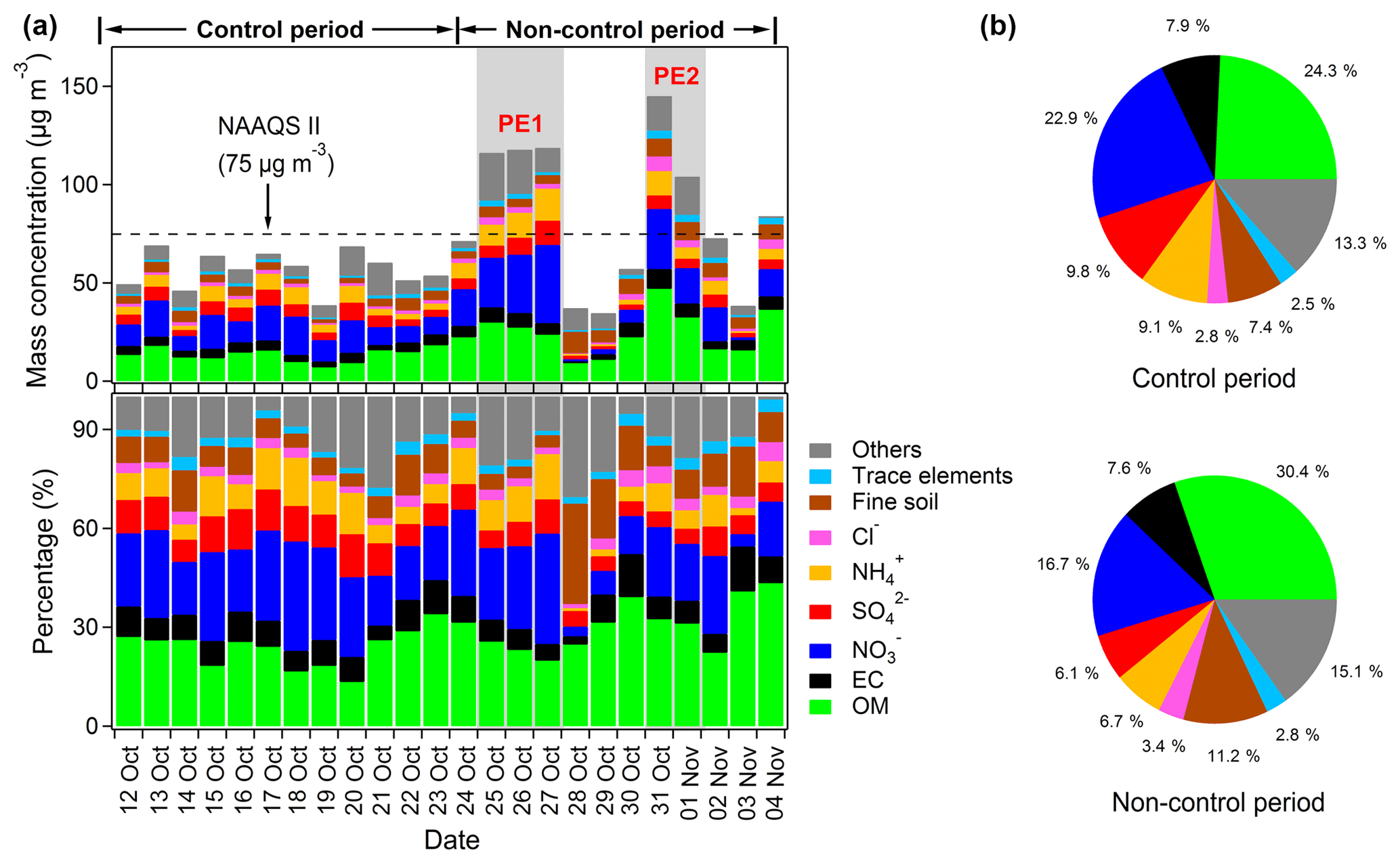
https://www.atmos-chem-phys.net/19/1881/2019/acp-19-1881-2019-f02

Figure 2(a) Daily variations in the contributions of chemical species to PM_2.5 mass during the campaign and (b) average contributions of chemical species during the NCCPC-control and non-control periods. PE1 and PE2 represent two pollution episodes.

Download

Table 1Summary of PM_2.5 and its major chemical components at Xianghe during the NCCPC-control and non-control periods.

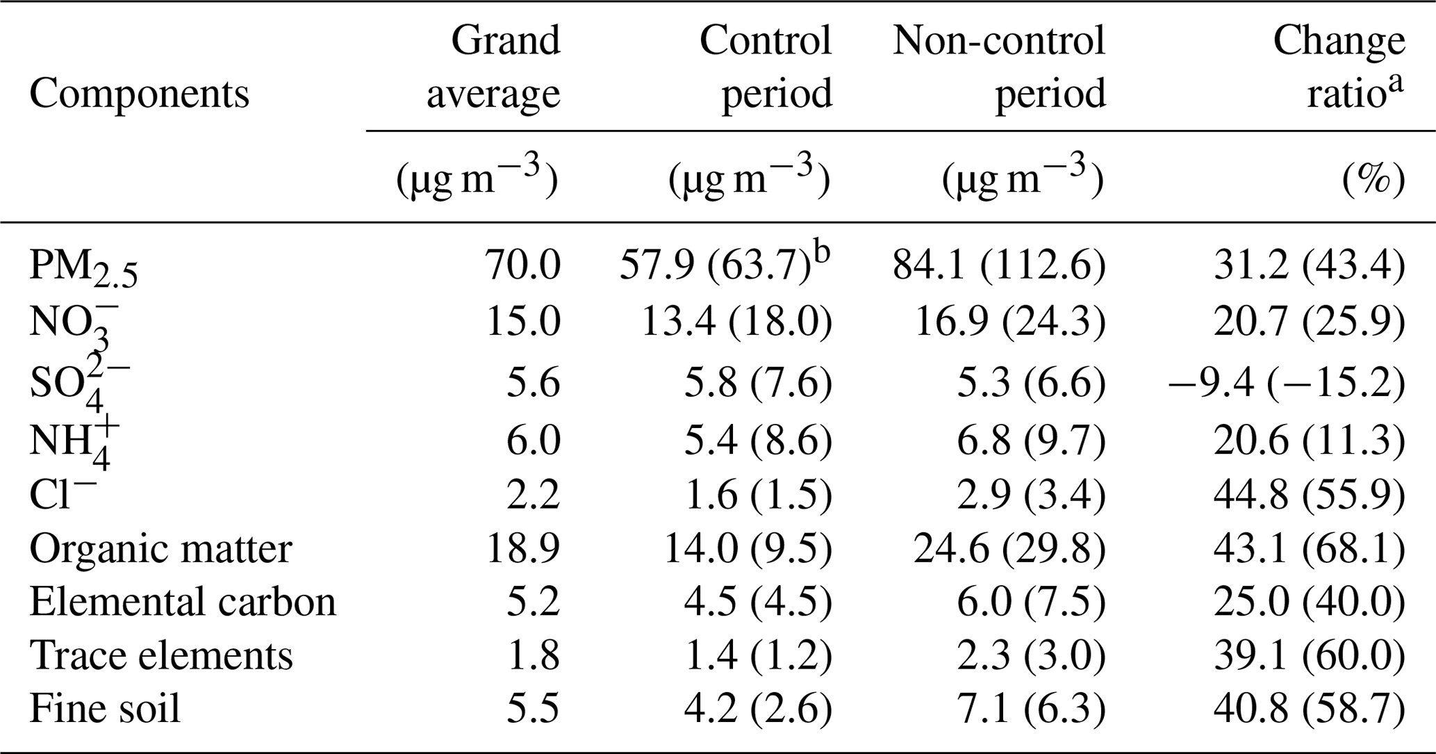
^a ([Non-control period]-[NCCPC-control period])/[Non-control period]. ^b Values in parentheses show the results for days with stable meteorological conditions (wind speed <0.4 m s⁻¹ and mixed-layer height <274 m).

Download Print Version | Download XLSX

As shown in Fig. 2b, the chemical-mass-closure calculations for PM_2.5 showed that on average OM was the largest contributor (30.4 %) to PM_2.5 mass during the non-control period, followed by ${NO}_{3}^{-}$ (16.7 %), fine soil (11.2 %), and EC (7.6 %). In contrast, OM (24.3 %) and ${NO}_{3}^{-}$ (22.9 %) dominated the PM_2.5 mass during the NCCPC-control period, followed by ${SO}_{4}^{2 -}$ (9.8 %), ${NH}_{4}^{+}$ (9.1 %), and EC (7.9 %). The OM mass concentration was decreased largely by 43.1 % from 24.6 µg m⁻³ during the non-control period to 14.0 µg m⁻³ during the NCCPC-control period. For secondary water-soluble inorganic ions, the average mass concentrations of ${NO}_{3}^{-}$ (13.4 µg m⁻³ versus 16.9 µg m⁻³) and ${NH}_{4}^{+}$ (5.4 versus 6.8 µg m⁻³) were lower by 20.7 % and 20.6 % during the NCCPC-control period, respectively. However, ${SO}_{4}^{2 -}$ exhibited similar loadings during the NCCPC-control (5.8 µg m⁻³) and non-control (5.3 µg m⁻³) periods. This is consistent with the small differences in SO₂ concentrations for the NCCPC-control (8.5 µg m⁻³, Fig. S4) versus the non-control (12.4 µg m⁻³, Fig. S4) periods. Indeed, the low SO₂ concentrations may not have provided sufficient gaseous precursor to form substantial amounts of sulfate. The loadings of EC, Cl⁻, and fine soil were lower by 25.0 %, 44.8 %, and 40.8 %, respectively, when the controls were in place. The variation in reductions for specific aerosol components imply differences in the effectiveness of the emission controls on the chemical species, but as discussed below, meteorological conditions probably had an influence on the loadings, too.

As shown in Fig. S4, both WSs (0.7±0.3 versus 1.3±0.8 m s⁻¹) and MLHs (304.3±60.6 versus 373.7±217.9 m) were lower for the NCCPC-control period compared with the non-control period. This indicates that horizontal and vertical dispersion were weaker during the NCCPC-control period than in the non-control period. More to the point, this shows that one needs to consider the effects of WS and MLH to fully evaluate the effectiveness of the pollution control measures. A simple and effective way to do this is to compare the concentrations of air pollutants for the two periods when atmospheric conditions were stable (Wang et al., 2015; Liang et al., 2017).

We first evaluated atmospheric stability based on relationships between PM_2.5 mass concentrations and WS and MLH. As shown in Fig. 3, the PM_2.5 mass concentrations exhibited a power function relationship with WS ( $r = - 0.65$ ) and MLH (r=0.77). The approach used to determine stable conditions was to find the WS and MLH values that were less than the inflection points in the PM_2.5 loadings; that is, where the slopes in the loadings changed from large to relatively small values. As there are no true inflection points for the power functions, we used piecewise functions to represent them. As shown in Fig. 3, the intersections of two linear regressions can be used to represent the inflection points of the influences of meteorological conditions on PM_2.5 mass. Using these criteria, days with WS<0.4 m s⁻¹ and MLH<274 m were subjectively considered to have stable atmospheric conditions.

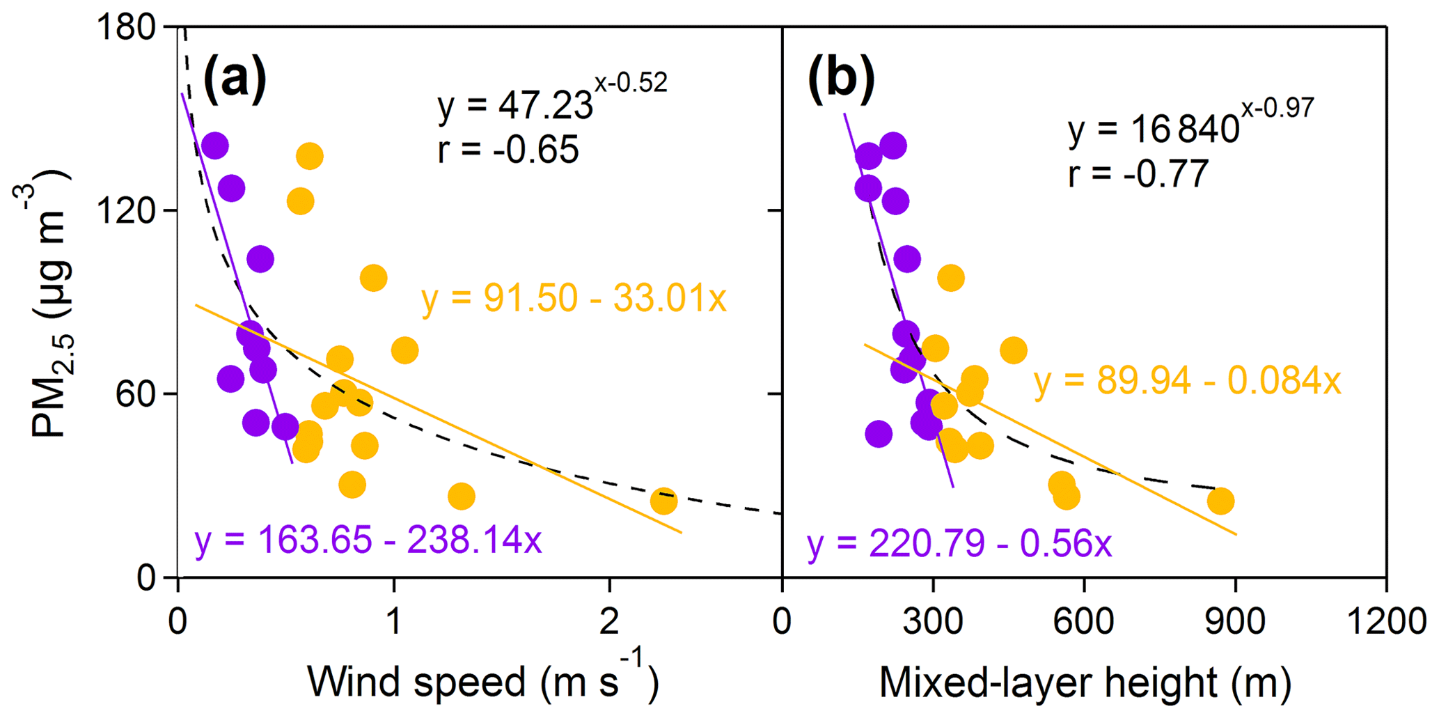
https://www.atmos-chem-phys.net/19/1881/2019/acp-19-1881-2019-f03

Figure 3Scatter plots showing the relationships between PM_2.5 mass concentrations and (a) wind speed and (b) mixed-layer height.

Download

There were 2 days for the NCCPC-control period and 3 days for the non-control period that satisfied the stability criteria. The surface charts (Fig. S5) show that the weather conditions for those selected stable atmosphere days during the NCCPC-control and non-control periods were mainly controlled by uniform pressure fields and weak low-pressure systems, respectively, and those conditions led to weak or calm surface winds. Due to the lower WS (0.2 versus 0.3 m s⁻¹) and MLH (213 versus 244 m) during the NCCPC-control period relative to the non-control period, the horizontal and vertical dispersion for the stable atmospheric days was slightly weaker during the NCCPC-control period. As shown in Table 1, the percentage differences for PM_2.5 (43.4 %), ${NO}_{3}^{-}$ (25.9 %), OM (68.1 %), EC (40.0 %), and fine soil (58.7 %) were larger for the days with stable atmospheric conditions compared with those for all days. These results are a further indication that the control measures were effective in reducing pollution, but meteorology also influenced the aerosol pollution.

3.2 Estimates of source contributions

The mass concentrations of water-soluble inorganic ions ( ${SO}_{4}^{2 -}$ , ${NO}_{3}^{-}$ , ${NH}_{4}^{+}$ , K⁺, and Cl⁻), carbonaceous species (OC and EC), and elements (Al, Si, Ca, Ti, Cr, Mn, Fe, Cu, Zn, As, Br, and Pb) were used as data inputs for the PMF 5.0 model. Through comparisons between the PMF profiles and reference profiles from previous studies, the presumptive sources for the aerosol were identified as (i) coal combustion, (ii) traffic-related emissions, (iii) secondary sources, (iv) biomass burning, (v) industrial processes, and (vi) mineral dust. As shown in Fig. S6, the PMF modeled PM_2.5 mass concentrations were strongly correlated with the observed values (r=0.98, slope=0.94), and the model-calculated concentrations for each chemical species exhibited good linearity and correlations with the measured values (r=0.68–0.99) (Table S1). These results show that the six identified sources were physically interpretable and accounted for much of the variability in the data.

Figure 4 presents the source profiles and the average contribution of each source to PM_2.5 mass during the NCCPC-control and non-control periods. The first source factor was identified as coal burning emissions because it was enriched with As (38.8 %), Pb (32.9 %), and Fe (30.3 %) and had moderate loadings of Mn (26.2 %), Zn (23.8 %), Si (23.1 %), and Ca (22.8 %) (Fig. 4a). Of these elements, As is a well-known tracer for coal burning (Hsu et al., 2009; Y. Chen et al., 2017); Pb, Fe, Mn, and Zn (Xu et al., 2012; Men et al., 2018) are enriched in particles generated by this source; and Ca and Si can be components of coal fly ash (Pipal et al., 2011). There was no significant difference in PM_2.5 loadings contributed by this source between the NCCPC-control (8.5 µg m⁻³) and non-control (7.8 µg m⁻³) periods. This may be because coal burning is mainly used for domestic purposes, especially heating, and the control measures did not include this sector. The contribution of coal burning to PM_2.5 mass in our October–November study was lower than its contribution in the BTH region in winter (∼20–60 µg m⁻³) (Huang et al., 2017), and that can be explained by the increased domestic usage of coal for heating activities during the colder winter season.

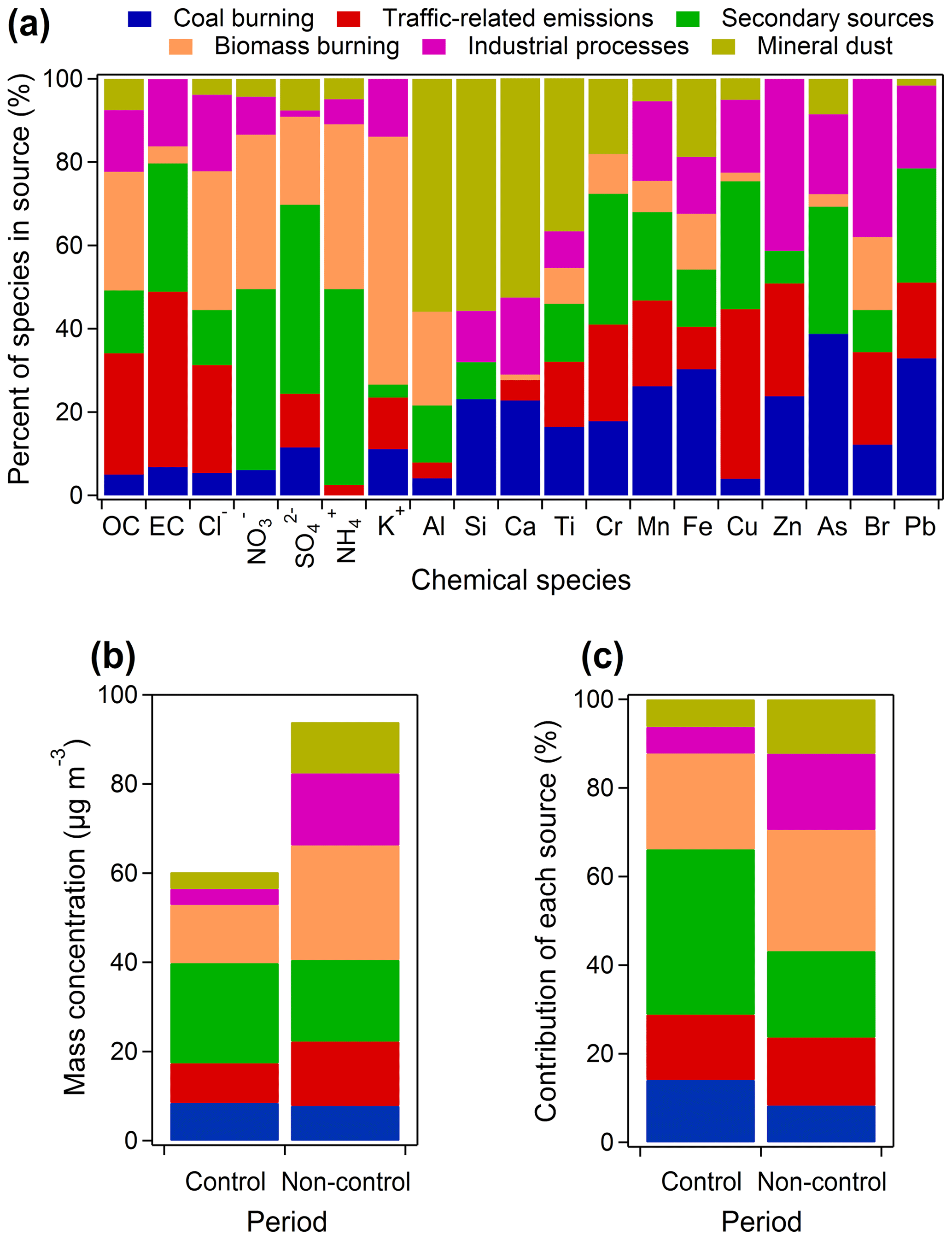
https://www.atmos-chem-phys.net/19/1881/2019/acp-19-1881-2019-f04

Figure 4(a) Source profiles for the six sources identified using the positive matrix factorization model version 5.0, (b) the mass concentrations of PM_2.5 contributed by each source, and (c) the average source contribution of each source to the PM_2.5 mass.

Download

The second source factor was linked to traffic-related emissions, and it was characterized by strong loadings of EC (42.1 %) and Cu (40.7 %) and moderate contributions of OC (29.1 %), Zn (27.1 %), and Br (22.2 %). Previous studies have indicated that carbonaceous aerosols are components of gasoline and diesel engine exhaust (Cao et al., 2005), and therefore EC and OC have been used as indicators for motor vehicle emissions (Chalbot et al., 2013; Khan et al., 2016a), and Br may also be emitted from internal combustion engines (Bukowiecki et al., 2005). Aerosol Cu and Zn are derived from other types of vehicle emissions, including those associated with lubricant and oil, brake linings, metal brake wear, and tires (Lin et al., 2015). Furthermore, the mass concentration of PM_2.5 from this source was strongly correlated (r=0.72) with vehicle-related NO_x concentrations (Fig. S7), which further suggests the validity of this PMF-resolved source. Traffic-related emissions showed similar percent contributions to PM_2.5 mass during the NCCPC-control (14.8 %) and non-control (15.4 %) periods (Fig. 4c), but the mass concentration was 38 % lower for the NCCPC-control period (8.9 µg m⁻³) than the non-control period (14.4 µg m⁻³). This shows that the reduction in motor vehicle activity during the NCCPC-control period led to better air quality.

The third source factor was a clear signal of secondary particle formation because it was dominated by high loadings of ${SO}_{4}^{2 -}$ (45.4 %), ${NO}_{3}^{-}$ (43.4 %), and ${NH}_{4}^{+}$ (47.0 %) (Zhang et al., 2013; Amil et al., 2016). Thus, this factor was assigned to the secondary sources. Moreover, moderate loadings of As (30.5 %), Pb (27.4 %), Cr (31.4 %), Cu (30.7 %), and EC (30.8 %) were also assigned to this factor, suggesting influences from coal burning and vehicle exhaust emissions. Although the concentrations of gaseous precursors, especially SO₂ and NO_x, were lower during the NCCPC-control period (Fig. S4), the average mass contribution of secondary PM_2.5 was larger when the controls were in effect (22.5 versus 18.3 µg m⁻³); indeed, this source was the largest contributing factor (37.3 % of PM_2.5 mass) during the NCCPC-control period. We note that the higher RH (84 %) during the NCCPC-control period compared with the non-control period (69 %) may have promoted the formation of the secondary inorganic aerosols through aqueous reactions (Sun et al., 2014).

The fourth source factor, identified as emissions from biomass burning, was characterized by the high loadings of K⁺ (59.5 %) and moderate loadings of Cl⁻ (33.3 %), OC (28.5 %), ${NO}_{3}^{-}$ (37.1 %), ${SO}_{4}^{2 -}$ (21.1 %), and ${NH}_{4}^{+}$ (39.6 %). Soluble K⁺ is an established tracer for biomass burning (Zhang et al., 2013; Wang et al., 2016b), and Cl⁻ and OC are also emitted during biomass burning (Tao et al., 2014; Huang et al., 2017). Previous studies have shown that SO₂ and NO₂ can be converted into sulfate and nitrate on KCl particles during the transport of biomass-burning emissions (Du et al., 2011). Therefore, the abundant ${NO}_{3}^{-}$ , ${SO}_{4}^{2 -}$ , and ${NH}_{4}^{+}$ associated with this factor may be indicative of aged biomass-burning particles. As shown in Fig. 4c, biomass burning contributed substantially to PM_2.5 mass during both the NCCPC (21.6 %) and non-control periods (27.3 %). This is to be expected because Hebei Province is a major corn and wheat producing area, and the residue of these crops are commonly used for residential cooking and heating or burned in the fields (J. Chen et al., 2017). The mass concentrations of PM_2.5 from this source were lower during the NCCPC (13.0 µg m⁻³) than in the non-control period (25.7 µg m⁻³), and this indicates the effectiveness of the control policy that forbade the open-space biomass burning during the NCCPC. As the control measures did not include prohibitions on the household use of biofuels, substantial contributions of biomass burning were still evident during the NCCPC-control period.

The fifth source factor was identified as emissions from industrial processes because it had high loadings of Zn (41.3 %), Br (38.0 %), Pb (19.9 %), As (19.2 %), Cu (17.5 %), and Mn (19.1 %) (Q. Q. Wang et al., 2017; Sammaritano et al., 2018). This source contributed 3.6 µg m⁻³ to PM_2.5 mass during the NCCPC-control period, which was lower than the non-control period (16.2 µg m⁻³) by 78 %, and its percent contribution to PM_2.5 mass also increased correspondingly from 6.0 % to 17.2 % after the controls were removed. The results showed that restrictions on industrial activities during the NCCPC-control period led to improvements in air quality. Iron and steel production are among the most important industries in BTH region, and the iron and steel production there accounted for 28.8 % of the total for China in 2016 (NBS, 2017). The sintering process in iron and steel industries produces large amounts of heavy metal pollutants: including Zn, Pb, and Mn (Duan and Tan, 2013). Hence, the iron and steel industries in the BTH region were probable sources for these metals during the non-control period.

The sixth source factor was obviously mineral dust because it had high loadings of Al (55.9 %), Si (55.7 %), Ca (52.6 %), and Ti (36.7 %) (Zhang et al., 2013; Tao et al., 2014; Kuang et al., 2015). This factor contributed 3.8 µg m⁻³ (6.3 % of PM_2.5 mass) during the NCCPC-control period and 11.5 µg m⁻³ (12.3 %) to PM_2.5 mass in the non-control period. Possible sources for the mineral dust include (i) natural dust, which contains crustal Al, Si, and Ti (Milando et al., 2016); (ii) construction dust, which includes Ca (Liu et al., 2017); and (iii) road dust, which is characterized by traffic-related species, such as Cu, Zn, Br, and EC (Khan et al., 2016b; Zong et al., 2016). Here, the mineral dust factor did not contain any notable contributions from the traffic-related species. Thus, this factor can be explained by the natural and construction dusts. As shown in Fig. S8, WS was positively correlated (r=0.75) with the PM_2.5 mass from mineral dust. To reduce the effects of wind speed on crustal dust resuspension, we compared the days with low winds (<1 m s⁻¹) during the sampling periods, and only three sampling days were excluded from the analysis. This comparison showed that the mass concentration of PM_2.5 from mineral dust was 60.0 % lower in the NCCPC-control period (3.8 µg m⁻³) compared with the non-control period (9.5 µg m⁻³). This was a strong indication that restrictions on construction activities during the NCCPC-control period were effective in reducing the mineral dust component of PM_2.5, but as noted above this was not a large component of the PM_2.5 mass.

3.3 Pollution episodes after the NCCPC-control period

As shown in Fig. 2a, two pollution episodes occurred after the NCCPC-control period (PE1: 25–27 October and PE2: 31 October–1 November); the average PM_2.5 mass concentrations in PE1 and PE2 were 117.5 and 124.5 µg m⁻³, respectively. For PE1, secondary sources were the dominant contributor to the fine particle population, accounting for 54.6 % of PM_2.5 mass (Fig. 5a), and the secondary species that showed the largest contribution to PM_2.5 mass was ${NO}_{3}^{-}$ (26.8 %) (Fig. 5b). The mass concentration of ${NO}_{3}^{-}$ increased from <10 µg m⁻³ before PE1 to >25 µg m⁻³ during the episode (Fig. 2). Molar ratios of ${NO}_{3}^{-}$ to NO₂ (NOR=n- ${NO}_{3}^{-}$ /(n-NO₂ + n- ${NO}_{3}^{-}$ )) were calculated to investigate nitrogen partitioning between the particulate and gas phases (Zhang et al., 2011). As shown in Fig. 6a, the mass concentration of PM_2.5 increased with NOR (r=0.65) throughout the entire campaign, which indicates that nitrate formation was involved in the high PM_2.5 loadings. The NORs ranged from 0.32 to 0.71 during the PE1, and those values were significantly different (t test, p<0.01) from the ratios before (0.23–0.29) or after PE1 (0.03–0.10), thus reflecting stronger nitrate formation during the pollution period. Furthermore, NOR exhibited an exponential increase with RH (r=0.80, Fig. 6b), and the higher RHs (91 %–93 %) during the PE1 may have led to greater aqueous nitrate production relative to the periods before (80 %–86 %) or after (33 %–57 %) the first pollution episode.

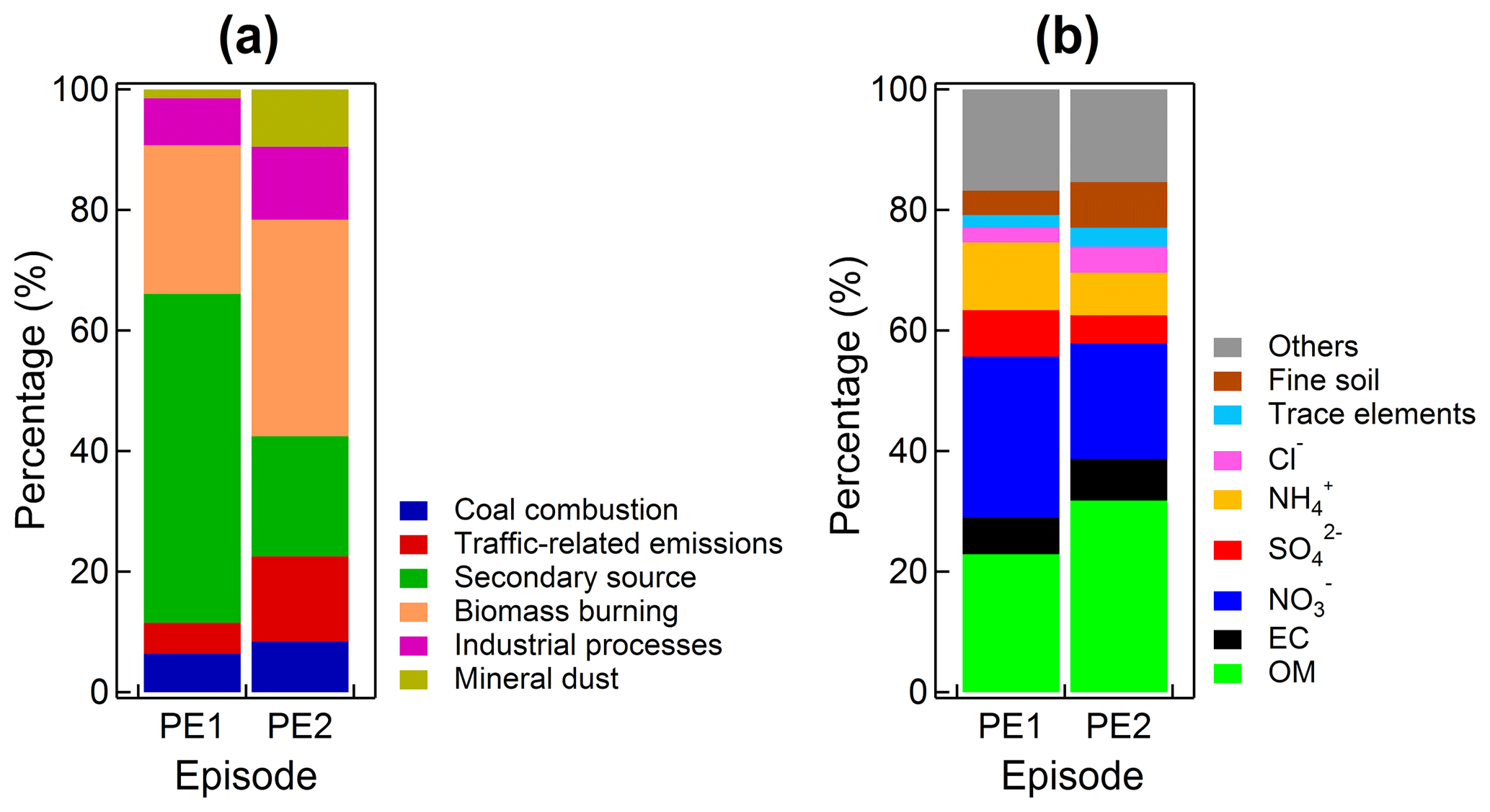
https://www.atmos-chem-phys.net/19/1881/2019/acp-19-1881-2019-f05

Figure 5Average source contributions of (a) each positive matrix factorization source factor and (b) chemical species to the PM_2.5 mass during two pollution episodes (PE1 and PE2).

Download

The second largest contributor to PM_2.5 mass during PE1 was OM, which accounted for 22.9 % of the fine aerosol mass. A widely used EC-tracer method (Lim and Turpin, 2002) was used to estimate the primary and secondary OA (POA and SOA). For this, the lowest 10 % percentile of the measured OC∕EC ratios was used as a measure of the primary OC∕EC ratio (Zheng et al., 2015). The estimated mass concentrations of POA and SOA were 17.2 and 9.7 µg m⁻³ during the PE1, which amounted to 63.9 % and 36.1 % of the OM mass, respectively.

Photochemical oxidation and aqueous reactions are two of the major mechanisms that lead to the formation of SOA (Hallquist et al., 2009), and we evaluated the roles of these chemical reactions by investigating trends in the EC-scaled concentrations of SOA (SOA∕EC). We note that normalizing the data in this way eliminates the impacts of different dilution and mixing conditions on the SOA loadings (Zheng et al., 2015). As shown in Fig. 6c, the SOA∕EC ratios increased (r=0.65) with O_x (NO₂+O₃), which is a proxy for atmospheric aging caused by photochemical reactions (Canonaco et al., 2015), and the EC-scaled concentrations showed a weaker correlation with RH ( $r = - 0.32$ ) (Fig. 6d). These results indicate that photochemical reactions rather than aqueous-phase oxidation were the major pathways for SOA formation. Thus, the small contribution of SOA to PM_2.5 during the PE1 may have been due to low photochemical activity during that episode.

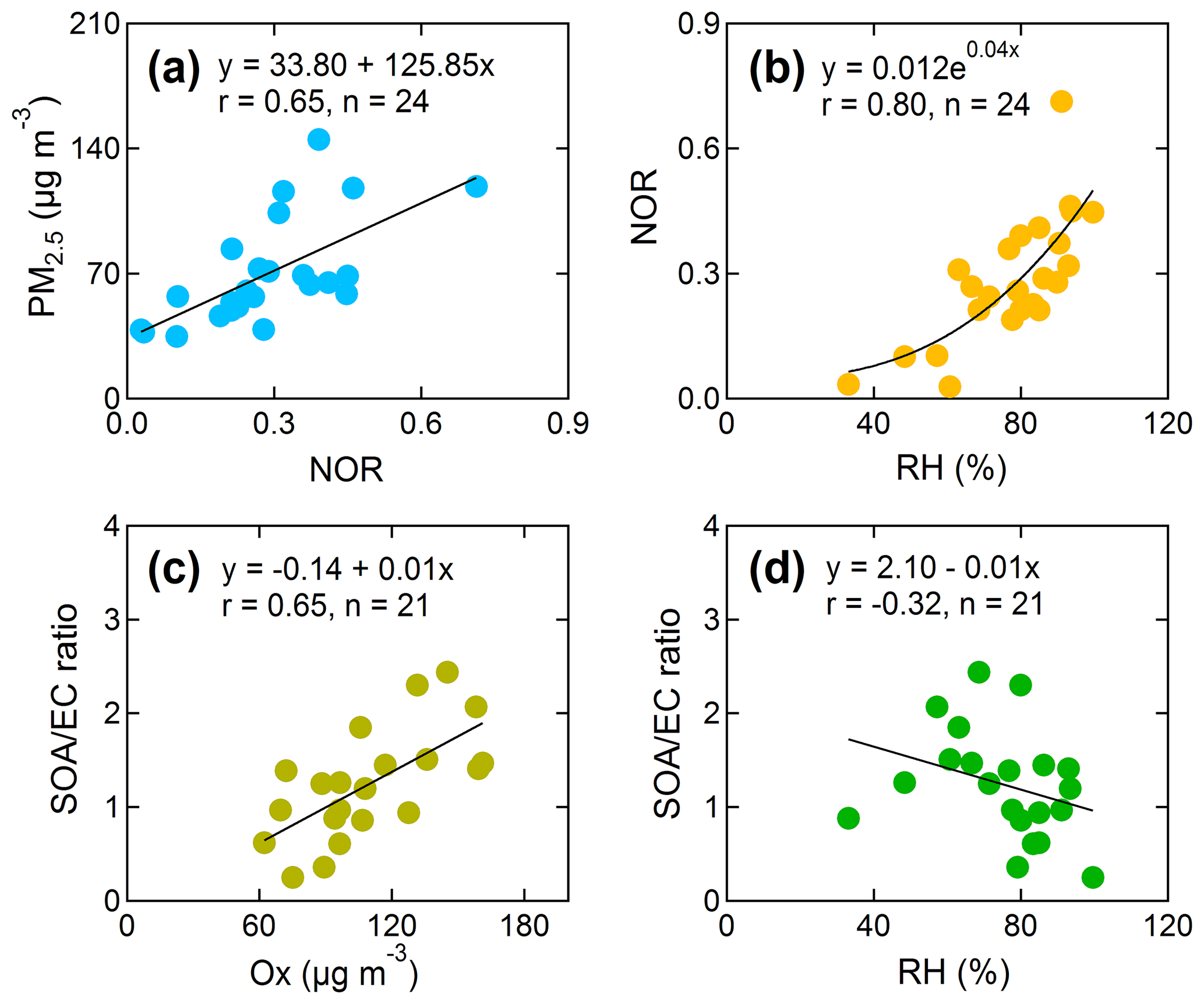
https://www.atmos-chem-phys.net/19/1881/2019/acp-19-1881-2019-f06

Figure 6Correlations for (a) PM_2.5 mass concentrations versus molar ratios of ${NO}_{3}^{-}$ and NO₂ (NOR), (b) NOR versus relative humidity (RH), (c) the ratio of secondary organic aerosol to elemental carbon (SOA∕EC) ratios versus O_x (O₃+NO₂), and (d) SOA∕EC versus RH for all samples from the campaign.

Download

In contrast to the first pollution episode, OM (31.8 %) was the most abundant PM_2.5 species during PE2, and that was followed by ${NO}_{3}^{-}$ (19.2 %) (Fig. 5b). The mass concentration of K⁺ increased substantially, from 0.1 µg m⁻³ before PE2 to 1.7 µg m⁻³ during the event, indicating a strengthening influence of biomass-burning emissions. Indeed, the results of PMF showed that biomass burning was the largest contributor to PM_2.5 mass during the PE2, accounting for 36.0 % of the total (Fig. 5a). Furthermore, the 72 h back trajectories showed that air masses sampled during the PE2 either originated from or passed over areas with fires in Inner Mongolia and Shanxi Province (see Fig. 7), and this can explain the apparent impacts from biomass-burning emissions. Moreover, SOA contributed an estimated 47.7 % of the OM mass, and that is a strong indication that secondary organics were a major component of the pollution. The mass concentration of SOA was 19.0 µg m⁻³ during the PE2, and that was higher than in 9.7 µg m⁻³ during the PE1. As the oxidizing conditions – as indicated by O_x – were similar for both pollution episodes (78.0 µg m⁻³ in PE1 versus 86.7 µg m⁻³ in PE2) (Fig. S4), the larger SOA during the PE2 can best be explained by SOA that formed from gaseous biomass-burning emissions during transport.

https://www.atmos-chem-phys.net/19/1881/2019/acp-19-1881-2019-f07

Figure 7The 3-day backward-in-time air mass trajectories (BT) arriving at 150 m above ground every hour from 31 October to 1 November 2017. The orange points represent fire counts that were derived from Moderate Resolution Imaging Spectroradiometer observations.

Download

3.4 Meteorological considerations

Previous studies have shown that meteorological conditions play an important role in the accumulation of pollution in the BTH region (Bei et al., 2017). Surface weather charts (Fig. 8) were used to analyze the synoptic conditions during the two pollution episodes, and the WRF-Chem model was applied to simulate the formation of PM_2.5 (Fig. 9). As shown in Figure S9, the predicted PM_2.5 and its major chemical components exhibited trends roughly similar to the observed values. The calculated MB and RMSE for PM_2.5 were −6.8 and 32.8 µg m⁻³, and the IOA was 0.75, indicating that the formation of PM_2.5 during the two pollution episodes was reasonably well captured by the WRF-Chem model even though the predicted average PM_2.5 mass concentration was lower than the observed value. The most probable reason for this is that uncertainties associated with the complex meteorological fields can affect the transport, diffusion, and removal of air pollutants in the atmosphere (Bei et al., 2012). Additionally, discrepancies in the emission inventories for PM_2.5 for different years may have contributed to the differences in modeled versus measured values.

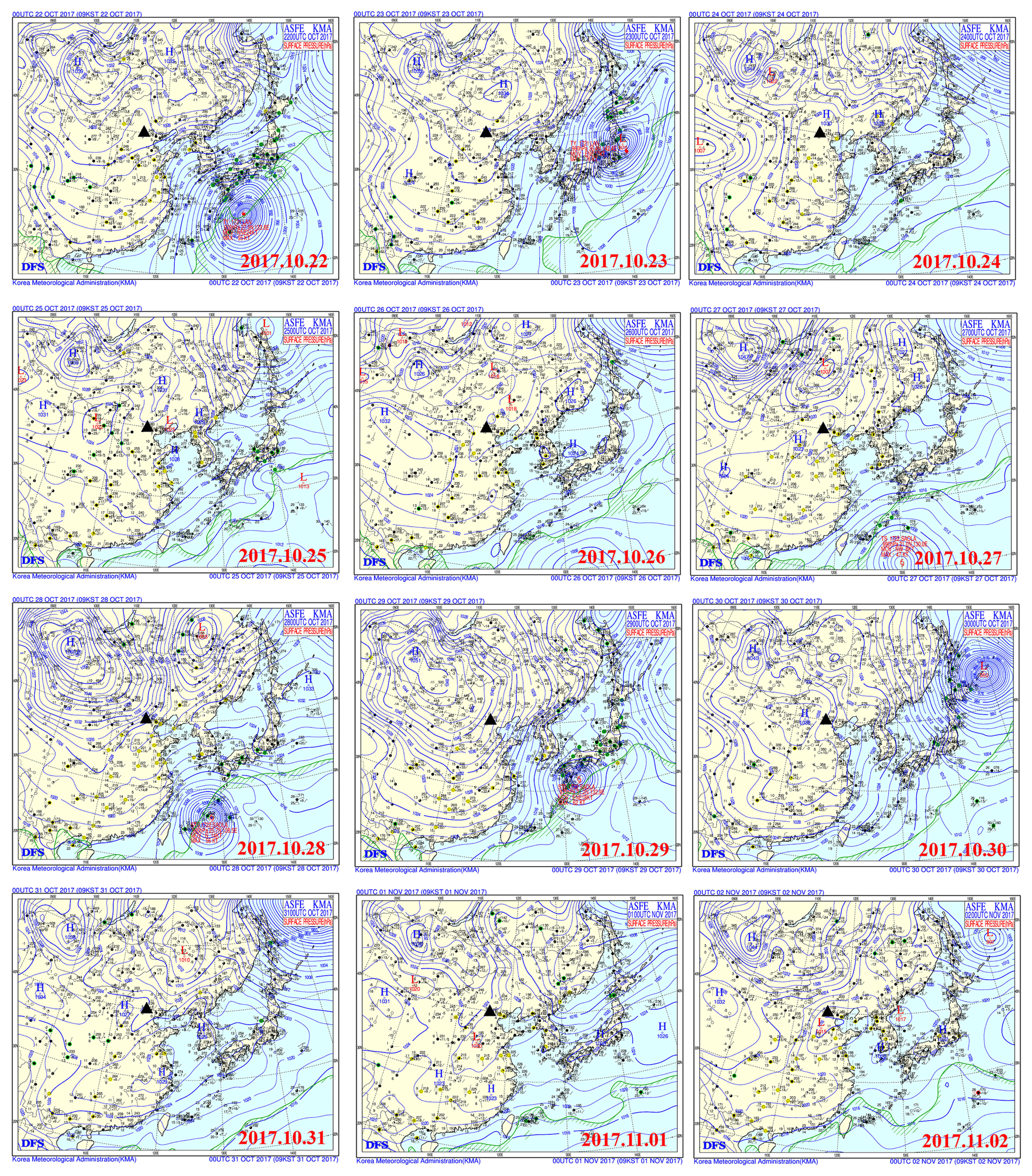
https://www.atmos-chem-phys.net/19/1881/2019/acp-19-1881-2019-f08

Figure 8Surface weather charts for 08:00 (local time) over East Asia from 22 October to 2 November 2017. The black triangles represent Xianghe.

On 22 October, that is, before PE1, a weak cold high-pressure system in Siberia moved southward (Fig. 8), and the BTH region was under the influence of a cold high-pressure system; conditions such as those tend to keep pollutants at low levels. After the passage of the low-pressure system, the BTH region was under the control of a weak high-pressure system from 24 to 25 October, and that led to a convergence of southerly airflow in the BTH region. Those meteorological conditions were favorable for the gradual accumulation of pollutants (Fig. 9). For example, as shown in Fig. S4, the NOx concentrations increased from 71.6 µg m⁻³ on 22 October to 147.6 µg m⁻³ on 25 October, and that increase provided a supply of gaseous precursors that can explain the observed large loadings of aerosol nitrate.

https://www.atmos-chem-phys.net/19/1881/2019/acp-19-1881-2019-f09

Figure 9Daily average PM_2.5 concentrations (µg m⁻³) simulated for the Beijing–Tianjin–Hebei region and surrounding areas from 25 October to 2 November 2017. The Weather Research and Forecasting model coupled to a chemistry (WRF-Chem) model was used for the simulation.

Download

On 28 October, the first day of PE1, cold air piled up in the BTH region, and the high-pressure system gradually strengthened. The weather in the BTH region at that time was characterized by cloudiness, high RH, and low surface WSs. Those conditions promoted the accumulation of pollutants (Fig. 9), and the WRF-Chem simulation indicated that the BTH region contributed 73.6 % of PM_2.5 mass during PE1. On 29 October, the cold high-pressure system moved towards the south, and northerly winds increased. Those meteorological conditions presumably led to a dilution of the air pollutants, and as a result, lower PM_2.5 loadings were observed in the BTH region (Fig. 9).

From 31 October to 1 November (PE2), the BTH region was again dominated by a weak high-pressure system, and a convergence of northerly airflow was caused by the high-pressure system and a trailing low-pressure front. Local pollutants from the BTH region would have accumulated under those conditions, but, as discussed above, the loadings of PM_2.5 also can be affected by the long-range transport processes. Indeed, the WRF-Chem simulation indicated that the BTH region contributed 46.9 % to PM_2.5 mass, similar to the import of fine particles from other regions (53.1 %). After 2 November, the cold high-pressure system began to move southward, the winds strengthened, and the air quality gradually improved.

3.5 Impacts of PM_2.5 emission reduction on aerosol radiative effects

The aerosol DRF refers to the change in the energy balance caused by the scattering and absorption of radiant energy by aerosols. As shown in Fig. S10, the reconstructed chemical b_scat correlated strongly (r=0.91) with the observed b_scat values; the slope of the linear regression was 0.90. This result indicates that the IMPROVE-based method provided a good estimation of the chemical b_scat; nonetheless, it is likely that more locally measured mass scattering efficiencies for each chemical species could reduce the underestimates of measured values. Moreover, a significant (p<0.01) relationship between the measured b_abs and EC mass (Fig. S2) validates the use of EC mass loadings in Eq. (12) to estimate the chemical b_abs. The contributions of each measured PM_2.5 component to the chemical b_ext were calculated based on Eq. (8), and, on average, OM was the largest contributor (43.5 %) to the chemical b_ext during the non-control period (Fig. 10a), followed by NH₄NO₃ (32.4 %), EC (14.3 %), (NH₄)₂SO₄ (7.6 %), and fine soil (2.2 %). In contrast, during the NCCPC-control period, NH₄NO₃ was the largest contributor to the chemical b_ext, amounting to 36.7 % of b_ext, and it was followed by OM (33.3 %), EC (16.2 %), (NH₄)₂SO₄ (11.9 %), and fine soil (1.9 %). The contributions of the various PM_2.5 components to b_ext were different compared with previous studies of the pollution controls for the Olympics and APEC. For example, Li et al. (2013) reported that (NH₄)₂SO₄ (41 %) had the largest contribution to b_ext during the Olympics, followed by NH₄NO₃ (23 %), OM (17 %), and EC (9 %); Zhou et al. (2017) found that OM (49 %) was the largest contributor to b_ext during the APEC summit, followed by NH₄NO₃ (19 %), (NH₄)₂SO₄ (13 %), and EC (12 %). These differences may be attributed to variable efficiencies of the controls for the specific fine particle species and to variations in RH among studies, the latter of which can influence sulfate and nitrate formation.

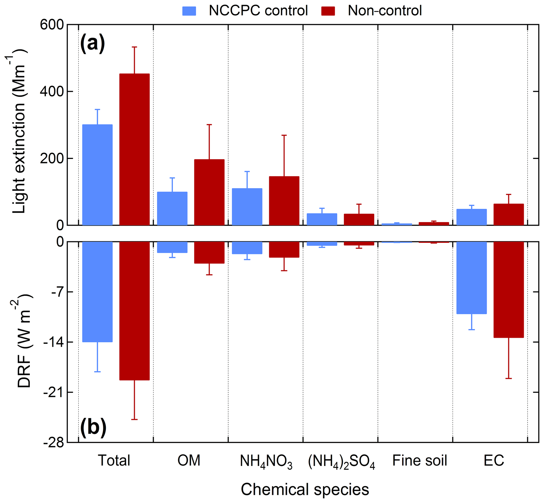
https://www.atmos-chem-phys.net/19/1881/2019/acp-19-1881-2019-f10

Figure 10Average values of (a) light extinction coefficients (including light scattering and absorption) and (b) direct radiative forcing (DRF) at the surface contributed by each PM_2.5 chemical composition during the NCCPC-control and non-control periods.

Download

As shown in Fig. S11, the AODs measured with a sun photometer were well correlated with the b_ext under ambient conditions; the slope (effective height) of the regression was 708 m and r=0.78. Based on the average effective height, the estimated chemical AOD (AOD = $708 \times b_{ext} \times 10^{- 6}$ ) and SSA contributed by each major component in PM_2.5 were entered into the TUV model to calculate the DRF at the Earth's surface. The estimated average DRF ranged from −33.2 to −3.4 W m⁻², with an arithmetic mean ± standard deviation of $- 16.5 \pm 6.7$ W m⁻² for the campaign. The average DRF for our study is similar to the −13.7 W m⁻² calculated for photosynthetically active radiation at Xianghe, China, in autumn using the Santa Barbara DISORT Atmospheric Radiative Transfer model (SBDART) (Xia et al., 2007a). Further comparisons with previous estimates of DRFs in China at ultraviolet and visible wavelengths show that the average value from our study is similar to that at the rural site of Taihu (−17.8 W m⁻², Xia et al., 2007b), but it was less negative than at the suburban or urban sites of Linan (−73.5 W m⁻², Xu et al., 2003), Nanjing (−39.4 W m⁻², Zhuang et al., 2014), or Xi'an (−100.5 W m⁻², Wang et al., 2016b). The more negative DRF values correspond with high aerosol loadings during those studies.

The estimated average DRF during the NCCPC-control period was $- 14.0 \pm 3.0$ W m⁻², which was less negative than the value during the non-control period ( $- 19.3 \pm 8.6$ W m⁻²) (Fig. 10b), and this is consistent with lower PM_2.5 mass loadings during the NCCPC-control period. Even though the DRF values were as high as −24.7 and −28.2 W m⁻² during PE1 and PE2, respectively, the percent reduction in DRF during the NCCPC-control period versus the non-control period (26.3 %) was smaller than the value during the APEC-control study (61.3 %, Zhou et al., 2017). Figure 10b also indicates that EC was responsible for the largest (most negative) DRF effects at the surface during the non-control period: the EC DRF value of −13.4 W m⁻² was followed by OM (−3.0 W m⁻²), NH₄NO₃ (−2.2 W m⁻²), (NH₄)₂SO₄ (−0.5 W m⁻²), and fine soil (−0.15 W m⁻²). The high EC DRF may have been due in part to EC particles being internally mixed with other materials because mixing can amplify light absorption and thereby increase DRF. The lower aerosol loadings during the NCCPC-control period can explain why the DRF values for EC, NH₄NO₃, OM, and fine soil in the uncontrolled period were smaller in magnitude: −10.1, −1.7, −1.6, and −0.09 W m⁻², respectively, than in the non-control period; these were equivalent to decreases of 24.6 %, 22.7 %, 46.7 %, and 40.0 %. These results suggest that the short-term mitigation measures implemented during the NCCPC reduced the cooling effects of PM_2.5 at the surface in Beijing.

4 Conclusions

We investigated the effects of pollution controls put in place during the 19th NCCPC on the chemical composition of PM_2.5 and aerosol radiative effects at the Earth's surface. The average mass concentration of PM_2.5 during the NCCPC-control period was 57.9±9.8 µg m⁻³, which was 31.2 % lower relative to the non-control period (84.1±38.84 µg m⁻³). The major chemical species, that is, OM, ${NO}_{3}^{-}$ , ${NH}_{4}^{+}$ , EC, and fine soil were lower by 43.1 %, 20.7 %, 20.6 %, 25.0 %, and 40.8 % during the NCCPC-control period, respectively, compared with samples taken after the controls were removed. Comparisons for only those days with stable meteorological conditions showed that the control versus non-control differences in PM_2.5 (43.4 %), ${NO}_{3}^{-}$ (25.9 %), OM (68.1 %), EC (40.0 %), and fine soil (58.7 %) were larger compared with those for all days. Overall, these results indicate that control measures were effective in reducing fine particle pollution.

Results of a PMF receptor model showed that biomass burning (27.3 %) was the largest contributor to PM_2.5 mass during the non-control period, followed by secondary sources (19.5 %), industrial processes (17.2 %), traffic-related emissions (15.4 %), mineral dust (12.3 %), and coal burning (8.3 %). In contrast, secondary sources (37.3 %) were the largest contributor to PM_2.5 mass during the NCCPC-control period, followed by biomass burning (21.6 %), traffic-related emissions (14.8 %), coal burning (14.1 %), mineral dust (6.3 %), and industrial processes (6.0 %). The mass concentrations of PM_2.5 contributed by traffic-related emissions, biomass burning, industrial processes, and mineral dust were all lower during the NCCPC-control period compared with the non-control period. However, there was no significant difference in PM_2.5 mass from coal burning between these two periods, and a larger PM_2.5 mass concentration of secondary sources was found for the NCCPC-control period.

There were two pollution episodes (PE1: 25–27 October and PE2: 31 October–1 November) that occurred after the NCCPC, and the average PM_2.5 mass concentrations during those events (117.5 µg m⁻³ for PE1 and 124.5 µg m⁻³ for PE2) were more than double those when the controls were in place. For PE1, secondary sources were the most important source for fine particles, accounting for 54.6 % of PM_2.5 mass. Aerosol ${NO}_{3}^{-}$ showed the largest contribution to PM_2.5 mass (26.8 %), and the high RH during PE1 likely promoted aqueous reactions involving nitrate. In contrast, OM (31.8 %) was the most abundant species in PM_2.5 during the PE2, and the PMF indicated that biomass burning was the largest source, accounting for 36.0 % of the PM_2.5 mass. The WRF-Chem simulation showed that the BTH region contributed 73.6 % and 46.9 % of PM_2.5 mass during the PE1 and PE2, respectively.

Calculations based on methods developed for the IMPROVE program indicated that OM was the largest contributor (43.5 %) to the chemical b_ext during the non-control period, followed by NH₄NO₃ (32.4 %), EC (14.3 %), (NH₄)₂SO₄ (7.6 %), and fine soil (2.2 %). During the NCCPC-control period, NH₄NO₃ accounted for 36.7 % of b_ext, and that was followed by OM (33.3 %), EC (16.2 %), (NH₄)₂SO₄ (11.9 %), and fine soil (1.9 %). The TUV model showed that the estimated average DRF ( $- 14.0 \pm 3.0$ W m⁻²) at the surface during the NCCPC-control period was 27.5 % less negative than in the non-control period ( $- 19.3 \pm 8.6$ W m⁻²), and this is consistent with the lower PM_2.5 loadings during the NCCPC-control period. Furthermore, EC had the largest (most negative) influence on DRF at the surface during the non-control period; the EC DRF value of −13.4 W m⁻² was followed by OM (−3.0 W m⁻²), NH₄NO₃ (−2.2 W m⁻²), (NH₄)₂SO₄ (−0.5 W m⁻²), and fine soil (−0.15 W m⁻²). The DRF values caused by EC, NH₄NO₃, OM, and fine soil when the controls were in place were lower by −10.1, −1.7, −1.6, and −0.09 W m⁻², respectively, compared with the non-control period, and the corresponding percent reductions were 24.6 %, 22.7 %, 46.7 %, and 40.0 %. The results suggest that the short-term mitigation measures during the NCCPC-control period were effective in reducing fine particle pollution and those actions also had radiative effects sufficient to affect surface temperature.

Data availability

All data described in this study are available upon request from the corresponding authors.

Supplement

The supplement related to this article is available online at: https://doi.org/10.5194/acp-19-1881-2019-supplement.

Author contributions

QW and JC designed the research. QW, SL, WD, YW, JT, YZ, and MW carried out the measurements. QW and NL performed the analysis and QW wrote the paper. All the authors commented on the paper.

Competing interests

The authors declare that they have no conflict of interest.

Special issue statement

This article is part of the special issue “Regional transport and transformation of air pollution in eastern China”. It is not associated with a conference.

Acknowledgements

This work was supported by the National Research Program for Key Issues in Air Pollution Control (DQGG0105) and the National Natural Science Foundation of China (41503118 and 41661144020). The authors are grateful to the staff from Xianghe Atmospheric Integrated Observatory for their assistance with field sampling.

Edited by: Luisa Molina
Reviewed by: Jianmin Chen and one anonymous referee

References

Amil, N., Latif, M. T., Khan, M. F., and Mohamad, M.: Seasonal variability of PM_2.5 composition and sources in the Klang Valley urban-industrial environment, Atmos. Chem. Phys., 16, 5357–5381, https://doi.org/10.5194/acp-16-5357-2016, 2016.

Bei, N., Li, G., and Molina, L. T.: Uncertainties in SOA simulations due to meteorological uncertainties in Mexico City during MILAGRO-2006 field campaign, Atmos. Chem. Phys., 12, 11295–11308, https://doi.org/10.5194/acp-12-11295-2012, 2012.

Bei, N., Wu, J., Elser, M., Feng, T., Cao, J., El-Haddad, I., Li, X., Huang, R., Li, Z., Long, X., Xing, L., Zhao, S., Tie, X., Prévôt, A. S. H., and Li, G.: Impacts of meteorological uncertainties on the haze formation in Beijing-Tianjin-Hebei (BTH) during wintertime: a case study, Atmos. Chem. Phys., 17, 14579–14591, https://doi.org/10.5194/acp-17-14579-2017, 2017.

Bukowiecki, N., Hill, M., Gehrig, R., Zwicky, C. N., Lienemann, P., Hegedüs, F., Falkenberg, G., Weingartner, E., and Baltensperger, U.: Trace metals in ambient air:? hourly size-segregated mass concentrations determined by synchrotron-XRF, Environ. Sci. Technol., 39, 5754–5762, https://doi.org/10.1021/es048089m, 2005.

Canonaco, F., Slowik, J. G., Baltensperger, U., and Prévôt, A. S. H.: Seasonal differences in oxygenated organic aerosol composition: implications for emissions sources and factor analysis, Atmos. Chem. Phys., 15, 6993–7002, https://doi.org/10.5194/acp-15-6993-2015, 2015.

Cao, J. J., Wang, Q. Y., Chow, J. C., Watson, J. G., Tie, X. X., Shen, Z. X., Wang, P., and An, Z. S.: Impacts of aerosol compositions on visibility impairment in Xi'an, China, Atmos. Environ., 59, 559–566, https://doi.org/10.1016/j.atmosenv.2012.05.036, 2012.

Cao, J. J., Lee, S. C., Ho, K. F., Zhang, X. Y., Zou, S. C., Fung, K., Chow, J. C., and Watson, J. G.: Characteristics of carbonaceous aerosol in Pearl River Delta Region, China during 2001 winter period, Atmos. Environ., 37, 1451–1460, https://doi.org/10.1016/S1352-2310(02)01002-6, 2003.

Cao, J. J., Wu, F., Chow, J. C., Lee, S. C., Li, Y., Chen, S. W., An, Z. S., Fung, K. K., Watson, J. G., Zhu, C. S., and Liu, S. X.: Characterization and source apportionment of atmospheric organic and elemental carbon during fall and winter of 2003 in Xi'an, China, Atmos. Chem. Phys., 5, 3127–3137, https://doi.org/10.5194/acp-5-3127-2005, 2005.

Chalbot, M.-C., McElroy, B., and Kavouras, I. G.: Sources, trends and regional impacts of fine particulate matter in southern Mississippi valley: significance of emissions from sources in the Gulf of Mexico coast, Atmos. Chem. Phys., 13, 3721–3732, https://doi.org/10.5194/acp-13-3721-2013, 2013.

Chen, J., Li, C., Ristovski, Z., Milic, A., Gu, Y., Islam, M. S., Wang, S., Hao, J., Zhang, H., He, C., Guo, H., Fu, H., Miljevic, B., Morawska, L., Thai, P., Lam, Y. F., Pereira, G., Ding, A., Huang, X., and Dumka, U. C.: A review of biomass burning: Emissions and impacts on air quality, health and climate in China, Sci. Total Environ., 579, 1000–1034, https://doi.org/10.1016/j.scitotenv.2016.11.025, 2017.

Chen, Y., Xie, S. D., Luo, B., and Zhai, C. Z.: Particulate pollution in urban Chongqing of southwest China: Historical trends of variation, chemical characteristics and source apportionment, Sci. Total Environ., 584–585, 523–534, https://doi.org/10.1016/j.scitotenv.2017.01.060, 2017.

Cheung, K., Daher, N., Shafer, M. M., Ning, Z., Schauer, J. J., and Sioutas, C.: Diurnal trends in coarse particulate matter composition in the Los Angeles Basin, J. Environ. Monit., 13, 3277–3287, https://doi.org/10.1039/c1em10296f, 2011.

Chow, J. C., Watson, J. G., Chen, L. W. A., Chang, M. C. O., Robinson, N. F., Trimble, D., and Kohl, S.: The IMPROVE_A Temperature Protocol for Thermal/Optical Carbon Analysis: Maintaining Consistency with a Long-Term Database, J. Air Waste Manage. Assoc., 57, 1014–1023, https://doi.org/10.3155/1047-3289.57.9.1014, 2007.

Draxler, R. R. and Rolph, G. D.: HYSPLIT (HYbrid Single-Particle Lagrangian Integrated Trajectory), Silver Spring, MD, Model access via NOAA ARL READY Website, available at: http://www.arl.noaa.gov/ready/hysplit4.htmlNOAAAirResourcesLaboratory (last access: February 2018), 2003.

Du, H., Kong, L., Cheng, T., Chen, J., Du, J., Li, L., Xia, X., Leng, C., and Huang, G.: Insights into summertime haze pollution events over Shanghai based on online water-soluble ionic composition of aerosols, Atmos. Environ., 45, 5131–5137, https://doi.org/10.1016/j.atmosenv.2011.06.027, 2011.

Duan, J. and Tan, J.: Atmospheric heavy metals and Arsenic in China: Situation, sources and control policies, Atmos. Environ., 74, 93–101, https://doi.org/10.1016/j.atmosenv.2013.03.031, 2013.

Elser, M., Huang, R.-J., Wolf, R., Slowik, J. G., Wang, Q., Canonaco, F., Li, G., Bozzetti, C., Daellenbach, K. R., Huang, Y., Zhang, R., Li, Z., Cao, J., Baltensperger, U., El-Haddad, I., and Prévôt, A. S. H.: New insights into PM_2.5 chemical composition and sources in two major cities in China during extreme haze events using aerosol mass spectrometry, Atmos. Chem. Phys., 16, 3207–3225, https://doi.org/10.5194/acp-16-3207-2016, 2016.

Emmons, L. K., Walters, S., Hess, P. G., Lamarque, J.-F., Pfister, G. G., Fillmore, D., Granier, C., Guenther, A., Kinnison, D., Laepple, T., Orlando, J., Tie, X., Tyndall, G., Wiedinmyer, C., Baughcum, S. L., and Kloster, S.: Description and evaluation of the Model for Ozone and Related chemical Tracers, version 4 (MOZART-4), Geosci. Model Dev., 3, 43–67, https://doi.org/10.5194/gmd-3-43-2010, 2010.

Feng, S. L., Gao, D., Liao, F., Zhou, F. R., and Wang, X. M.: The health effects of ambient PM_2.5 and potential mechanisms, Ecotox. Environ. Safe., 128, 67–74, https://doi.org/10.1016/j.ecoenv.2016.01.030, 2016.

Gao, Y., Liu, X., Zhao, C., and Zhang, M.: Emission controls versus meteorological conditions in determining aerosol concentrations in Beijing during the 2008 Olympic Games, Atmos. Chem. Phys., 11, 12437–12451, https://doi.org/10.5194/acp-11-12437-2011, 2011.

Guo, S., Hu, M., Guo, Q., Zhang, X., Schauer, J. J., and Zhang, R.: Quantitative evaluation of emission controls on primary and secondary organic aerosol sources during Beijing 2008 Olympics, Atmos. Chem. Phys., 13, 8303–8314, https://doi.org/10.5194/acp-13-8303-2013, 2013.

Hallquist, M., Wenger, J. C., Baltensperger, U., Rudich, Y., Simpson, D., Claeys, M., Dommen, J., Donahue, N. M., George, C., Goldstein, A. H., Hamilton, J. F., Herrmann, H., Hoffmann, T., Iinuma, Y., Jang, M., Jenkin, M. E., Jimenez, J. L., Kiendler-Scharr, A., Maenhaut, W., McFiggans, G., Mentel, Th. F., Monod, A., Prévôt, A. S. H., Seinfeld, J. H., Surratt, J. D., Szmigielski, R., and Wildt, J.: The formation, properties and impact of secondary organic aerosol: current and emerging issues, Atmos. Chem. Phys., 9, 5155–5236, https://doi.org/10.5194/acp-9-5155-2009, 2009.

Han, X., Guo, Q., Liu, C., Strauss, H., Yang, J., Hu, J., Wei, R., Tian, L., Kong, J., and Peters, M.: Effect of the pollution control measures on PM_2.5 during the 2015 China Victory Day Parade: Implication from water-soluble ions and sulfur isotope, Environ. Pollut., 218, 230–241, https://doi.org/10.1016/j.envpol.2016.06.038, 2016.

Hsu, S.-C., Liu, S. C., Huang, Y.-T., Chou, C. C. K., Lung, S. C. C., Liu, T.-H., Tu, J.-Y., and Tsai, F.: Long-range southeastward transport of Asian biosmoke pollution: Signature detected by aerosol potassium in Northern Taiwan, J. Geophys. Res.-Atmos., 114, D14301, https://doi.org/10.1029/2009JD011725, 2009.

Huang, X., Liu, Z., Liu, J., Hu, B., Wen, T., Tang, G., Zhang, J., Wu, F., Ji, D., Wang, L., and Wang, Y.: Chemical characterization and source identification of PM_2.5 at multiple sites in the Beijing-Tianjin-Hebei region, China, Atmos. Chem. Phys., 17, 12941–12962, https://doi.org/10.5194/acp-17-12941-2017, 2017.

Khan, M. F., Sulong, N. A., Latif, M. T., Nadzir, M. S. M., Amil, N., Hussain, D. F. M., Lee, V., Hosaini, P. N., Shaharom, S., Yusoff, N. A. Y. M., Hoque, H. M. S., Chung, J. X., Sahani, M., Mohd Tahir, N., Juneng, L., Maulud, K. N. A., Abdullah, S. M. S., Fujii, Y., Tohno, S., and Mizohata, A.: Comprehensive assessment of PM_2.5 physicochemical properties during the Southeast Asia dry season (southwest monsoon), J. Geophys. Res.-Atmos., 121, 14589–14611, https://doi.org/10.1002/2016JD025894, 2016a.

Khan, M. F., Latif, M. T., Saw, W. H., Amil, N., Nadzir, M. S. M., Sahani, M., Tahir, N. M., and Chung, J. X.: Fine particulate matter in the tropical environment: monsoonal effects, source apportionment, and health risk assessment, Atmos. Chem. Phys., 16, 597–617, https://doi.org/10.5194/acp-16-597-2016, 2016b.

Kuang, B. Y., Lin, P., Huang, X. H. H., and Yu, J. Z.: Sources of humic-like substances in the Pearl River Delta, China: positive matrix factorization analysis of PM_2.5 major components and source markers, Atmos. Chem. Phys., 15, 1995–2008, https://doi.org/10.5194/acp-15-1995-2015, 2015.

Lecoeur, E., Seigneur, C., Page, C., and Terray, L.: A statistical method to estimate PM_2.5 concentrations from meteorology and its application to the effect of climate change, J. Geophys. Res.-Atmos., 119, 3537–3585, https://doi.org/10.1002/2013JD021172, 2014.

Li, G., Bei, N., Tie, X., and Molina, L. T.: Aerosol effects on the photochemistry in Mexico City during MCMA-2006/MILAGRO campaign, Atmos. Chem. Phys., 11, 5169–5182, https://doi.org/10.5194/acp-11-5169-2011, 2011a.

Li, G., Zavala, M., Lei, W., Tsimpidi, A. P., Karydis, V. A., Pandis, S. N., Canagaratna, M. R., and Molina, L. T.: Simulations of organic aerosol concentrations in Mexico City using the WRF-CHEM model during the MCMA-2006/MILAGRO campaign, Atmos. Chem. Phys., 11, 3789–3809, https://doi.org/10.5194/acp-11-3789-2011, 2011b.

Li, G., Lei, W., Bei, N., and Molina, L. T.: Contribution of garbage burning to chloride and PM_2.5 in Mexico City, Atmos. Chem. Phys., 12, 8751–8761, https://doi.org/10.5194/acp-12-8751-2012, 2012.

Li, J., Xie, S. D., Zeng, L. M., Li, L. Y., Li, Y. Q., and Wu, R. R.: Characterization of ambient volatile organic compounds and their sources in Beijing, before, during, and after Asia-Pacific Economic Cooperation China 2014, Atmos. Chem. Phys., 15, 7945–7959, https://doi.org/10.5194/acp-15-7945-2015, 2015.

Li, J. and Han, Z.: A modeling study of severe winter haze events in Beijing and its neighboring regions, Atmos. Res., 170, 87–97, https://doi.org/10.1016/j.atmosres.2015.11.009, 2016.

Li, X., He, K., Li, C., Yang, F., Zhao, Q., Ma, Y., Cheng, Y., Ouyang, W., and Chen, G.: PM_2.5 mass, chemical composition, and light extinction before and during the 2008 Beijing Olympics, J. Geophys. Res.-Atmos., 118, 12158–12167, https://doi.org/10.1002/2013JD020106, 2013.

Liang, P., Zhu, T., Fang, Y., Li, Y., Han, Y., Wu, Y., Hu, M., and Wang, J.: The role of meteorological conditions and pollution control strategies in reducing air pollution in Beijing during APEC 2014 and Victory Parade 2015, Atmos. Chem. Phys., 17, 13921–13940, https://doi.org/10.5194/acp-17-13921-2017, 2017.

Lim, H.-J. and Turpin, B. J.: Origins of primary and secondary organic aerosol in Atlanta? Results of time-resolved measurements during the Atlanta Supersite Experiment, Environ. Sci. Technol., 36, 4489–4496, https://doi.org/10.1021/es0206487, 2002.

Lin, H., Liu, T., Fang, F., Xiao, J., Zeng, W., Li, X., Guo, L., Tian, L., Schootman, M., Stamatakis, K. A., Qian, Z., and Ma, W.: Mortality benefits of vigorous air quality improvement interventions during the periods of APEC Blue and Parade Blue in Beijing, China, Environ. Pollut., 220, 222–227, https://doi.org/10.1016/j.envpol.2016.09.041, 2017.

Lin, Y.-C., Tsai, C.-J., Wu, Y.-C., Zhang, R., Chi, K.-H., Huang, Y.-T., Lin, S.-H., and Hsu, S.-C.: Characteristics of trace metals in traffic-derived particles in Hsuehshan Tunnel, Taiwan: size distribution, potential source, and fingerprinting metal ratio, Atmos. Chem. Phys., 15, 4117–4130, https://doi.org/10.5194/acp-15-4117-2015, 2015.

Liu, B., Wu, J., Zhang, J., Wang, L., Yang, J., Liang, D., Dai, Q., Bi, X., Feng, Y., Zhang, Y., and Zhang, Q.: Characterization and source apportionment of PM_2.5 based on error estimation from EPA PMF 5.0 model at a medium city in China, Environ. Pollut., 222, 10–22, https://doi.org/10.1016/j.envpol.2017.01.005, 2017.

Madronich, S.: UV radiation in the natural and perturbed atmosphere, In: M. Tevini, Ed., UV-B Radiation and Ozone Depletion, Lewis Publishers, London, 17–69, 1993.

Malm William, C., Day Derek, E., Kreidenweis Sonia, M., Collett Jeffrey, L., and Lee, T.: Humidity-dependent optical properties of fine particles during the Big Bend Regional Aerosol and Visibility Observational Study, J. Geophys. Res.-Atmos., 108, 4279, https://doi.org/10.1029/2002JD002998, 2003.

Men, C., Liu, R., Xu, F., Wang, Q., Guo, L., and Shen, Z.: Pollution characteristics, risk assessment, and source apportionment of heavy metals in road dust in Beijing, China, Sci. Total Environ., 612, 138–147, https://doi.org/10.1016/j.scitotenv.2017.08.123, 2018.

Milando, C., Huang, L., and Batterman, S.: Trends in PM_2.5 emissions, concentrations and apportionments in Detroit and Chicago, Atmos. Environ., 129, 197–209, https://doi.org/10.1016/j.atmosenv.2016.01.012, 2016.

National Bureau of Statistics (NBS): China Statistical Yearbook 2013, China Statistics Press, Beijing, 2013a (in Chinese).

Norris, G., Duvall, R., Brown, S., and Bai, S.: EPA Positive Matrix Factorization (PMF) 5.0 fundamentals and User Guide Prepared for the US Environmental Protection Agency Office of Research and Development, Washington, DC, Inc., Petaluma, 2014.

Paatero, P. and Tapper, U.: Positive matrix factorization: A non-negative factor model with optimal utilization of error estimates of data values, Environmetrics, 5, 111–126, https://doi.org/10.1002/env.3170050203, 2006.

Palancar, G. G. and Toselli, B. M.: Effects of meteorology and tropospheric aerosols on UV-B radiation: a 4-year study, Atmos. Environ., 38, 2749–2757, https://doi.org/10.1016/j.atmosenv.2004.01.036, 2004.

Pipal, A. S., Kulshrestha, A., and Taneja, A.: Characterization and morphological analysis of airborne PM_2.5 and PM₁₀ in Agra located in north central India, Atmos. Environ., 45, 3621–3630, https://doi.org/10.1016/j.atmosenv.2011.03.062, 2011.

Pitchford, M., Malm, W., Schichtel, B., Kumar, N., Lowenthal, D., and Hand, J.: Revised algorithm for estimating light extinction from IMPROVE particle speciation data, J. Air Waste Manage. Assoc., 57, 1326–1336, https://doi.org/10.3155/1047-3289.57.11.1326, 2007.

Pui, D. Y. H., Chen, S. C., and Zuo, Z. L.: PM_2.5 in China: Measurements, sources, visibility and health effects, and mitigation, Particuology, 13, 1–26, https://doi.org/10.1016/j.partic.2013.11.001, 2014.

Ran, L., Deng, Z. Z., Wang, P. C., and Xia, X. A.: Black carbon and wavelength-dependent aerosol absorption in the North China Plain based on two-year aethalometer measurements, Atmos. Environ., 142, 132–144, https://doi.org/10.1016/j.atmosenv.2016.07.014, 2016.

Sammaritano, M. A., Bustos, D. G., Poblete, A. G., and Wannaz, E. D.: Elemental composition of PM_2.5 in the urban environment of San Juan, Argentina, Environ. Sci. Pollut. Res., 25, 4197–4203, https://doi.org/10.1007/s11356-017-0793-5, 2018.

Sun, Y., Jiang, Q., Wang, Z., Fu, P., Li, J., Yang, T., and Yin, Y.: Investigation of the sources and evolution processes of severe haze pollution in Beijing in January 2013, J. Geophys. Res.-Atmos., 119, 4380–4398, https://doi.org/10.1002/2014JD021641, 2014.

Tang, G., Zhu, X., Hu, B., Xin, J., Wang, L., Münkel, C., Mao, G., and Wang, Y.: Impact of emission controls on air quality in Beijing during APEC 2014: lidar ceilometer observations, Atmos. Chem. Phys., 15, 12667–12680, https://doi.org/10.5194/acp-15-12667-2015, 2015.

Tao, J., Gao, J., Zhang, L., Zhang, R., Che, H., Zhang, Z., Lin, Z., Jing, J., Cao, J., and Hsu, S. C.: PM_2.5 pollution in a megacity of southwest China: source apportionment and implication, Atmos. Chem. Phys., 14, 8679–8699, https://doi.org/10.5194/acp-14-8679-2014, 2014.

Tao, J., Gao, J., Zhang, L., Wang, H., Qiu, X., Zhang, Z., Wu, Y., Chai, F., and Wang, S.: Chemical and optical characteristics of atmospheric aerosols in Beijing during the Asia-Pacific Economic Cooperation China 2014, Atmos. Environ., 144, 8–16, https://doi.org/10.1016/j.atmosenv.2016.08.067, 2016.

Tao, J., Zhang, L. M., Cao, J. J., and Zhang, R. J.: A review of current knowledge concerning PM_2.5 chemical composition, aerosol optical properties and their relationships across China, Atmos. Chem. Phys., 17, 9485–9518, https://doi.org/10.5194/acp-17-9485-2017, 2017.

Tie, X., Huang, R.-J., Dai, W., Cao, J., Long, X., Su, X., Zhao, S., Wang, Q., and Li, G.: Effect of heavy haze and aerosol pollution on rice and wheat productions in China, Sci. Rep., 6, 29612, https://doi.org/10.1038/srep29612, 2016.

Wang, J., Wang, G., Gao, J., Wang, H., Ren, Y., Li, J., Zhou, B., Wu, C., Zhang, L., Wang, S., and Chai, F.: Concentrations and stable carbon isotope compositions of oxalic acid and related SOA in Beijing before, during, and after the 2014 APEC, Atmos. Chem. Phys., 17, 981–992, https://doi.org/10.5194/acp-17-981-2017, 2017.

Wang, Q. Q., He, X., Huang, X. H. H., Griffith, S. M., Feng, Y., Zhang, T., Zhang, Q., Wu, D., and Yu, J. Z.: Impact of secondary organic aerosol tracers on tracer-based source apportionment of organic carbon and PM_2.5: A case study in the Pearl River Delta, China, Earth Space Chem., 1, 562–571, https://doi.org/10.1021/acsearthspacechem.7b00088, 2017.

Wang, Q. Y., Huang, R.-J., Cao, J., Tie, X., Shen, Z., Zhao, S., Han, Y., Li, G., Li, Z., Ni, H., Zhou, Y., Wang, M., Chen, Y., and Su, X.: Contribution of regional transport to the black carbon aerosol during winter haze period in Beijing, Atmos. Environ., 132, 11–18, https://doi.org/10.1016/j.atmosenv.2016.02.031, 2016a.

Wang, Q. Y., Huang, R.-J., Zhao, Z., Cao, J., Ni, H., Tie, X., Zhao, S., Su, X., Han, Y., Shen, Z., Wang, Y., Zhang, N., Zhou, Y., and Corbin, J. C.: Physicochemical characteristics of black carbon aerosol and its radiative impact in a polluted urban area of China, J. Geophys. Res.-Atmos., 121, 12505–12519, https://doi.org/10.1002/2016JD024748, 2016b.

Wang, Q. Y., Cao, J., Han, Y., Tian, J., Zhang, Y., Pongpiachan, S., Zhang, Y., Li, L., Niu, X., Shen, Z., Zhao, Z., Tipmanee, D., Bunsomboonsakul, S., Chen, Y., and Sun, J.: Enhanced light absorption due to the mixing state of black carbon in fresh biomass burning emissions, Atmos. Environ., 180, 184–191, https://doi.org/10.1016/j.atmosenv.2018.02.049, 2018a.

Wang, Q., Cao, J., Han, Y., Tian, J., Zhu, C., Zhang, Y., Zhang, N., Shen, Z., Ni, H., Zhao, S., and Wu, J.: Sources and physicochemical characteristics of black carbon aerosol from the southeastern Tibetan Plateau: internal mixing enhances light absorption, Atmos. Chem. Phys., 18, 4639–4656, https://doi.org/10.5194/acp-18-4639-2018, 2018b.

Wang, S., Zhao, M., Xing, J., Wu, Y., Zhou, Y., Lei, Y., He, K., Fu, L., and Hao, J.: Quantifying the air pollutants emission reduction during the 2008 Olympic Games in Beijing, Environ. Sci. Technol., 44, 2490–2496, https://doi.org/10.1021/es9028167, 2010.

Wang, W., Primbs, T., Tao, S., and Simonich, S. L. M.: Atmospheric particulate matter pollution during the 2008 Beijing Olympics, Environ. Sci. Technol., 43, 5314–5320, https://doi.org/10.1021/es9007504, 2009.

Wang, Z., Li, Y., Chen, T., Li, L., Liu, B., Zhang, D., Sun, F., Wei, Q., Jiang, L., and Pan, L.: Changes in atmospheric composition during the 2014 APEC conference in Beijing, J. Geophys. Res.-Atmos., 120, 12695–12707, https://doi.org/10.1002/2015JD023652, 2015.

Watson, J. G.: Visibility: Science and regulation, J. Air Waste Manage. Assoc., 52, 628–713, https://doi.org/10.1080/10473289.2002.10470813, 2002.

Xia, X., Li, Z., Wang, P., Chen, H., and Cribb, M.: Estimation of aerosol effects on surface irradiance based on measurements and radiative transfer model simulations in northern China, J. Geophys. Res.-Atmos., 112, D22S10, https://doi.org/10.1029/2006JD008337, 2007a.

Xia, X., Li, Z, Holben, B., Wang, P., Eck, T., Chen, H., Cribb, M., and Zhao, Y.: Aerosol optical properties and radiative effects in the Yangtze Delta region of China, J. Geophys. Res.-Atmos., 112, D22S12, https://doi.org/10.1029/2007JD008859, 2007b.

Xiao, S., Wang, Q., Cao, J., Huang, R.-J., Chen, W., Han, Y., Xu, H., Liu, S., Zhou, Y., and Wang, P.: Long-term trends in visibility and impacts of aerosol composition on visibility impairment in Baoji, China, Atmos. Res., 149, 88–95, https://doi.org/10.1016/j.atmosres.2014.06.006, 2014.

Xie, R., Sabel, C. E., Lu, X., Zhu, W. M., Kan, H. D., Nielsen, C. P., and Wang, H. K.: Long-term trend and spatial pattern of PM_2.5 induced premature mortality in China, Environ. Int., 97, 180–186, https://doi.org/10.1016/j.envint.2016.09.003, 2016.

Xu, H. M., Cao, J. J., Ho, K. F., Ding, H., Han, Y. M., Wang, G. H., Chow, J. C., Watson, J. G., Khol, S. D., Qiang, J., and Li, W. T.: Lead concentrations in fine particulate matter after the phasing out of leaded gasoline in Xi'an, China, Atmos. Environ., 46, 217–224, https://doi.org/10.1016/j.atmosenv.2011.09.078, 2012.

Xu, J., Bergin, M. H., and Greenwald, R.: Direct aerosol radiative forcing in the Yangtze delta region of China: Observation and model estimation, J. Geophys. Res.-Atmos., 108, 4060, https://doi.org/10.1029/2002JD002550, 2003.

Xu, W., Song, W., Zhang, Y., Liu, X., Zhang, L., Zhao, Y., Liu, D., Tang, A., Yang, D., Wang, D., Wen, Z., Pan, Y., Fowler, D., Collett Jr., J. L., Erisman, J. W., Goulding, K., Li, Y., and Zhang, F.: Air quality improvement in a megacity: implications from 2015 Beijing Parade Blue pollution control actions, Atmos. Chem. Phys., 17, 31–46, https://doi.org/10.5194/acp-17-31-2017, 2017.

Xu, W. Q., Sun, Y. L., Chen, C., Du, W., Han, T. T., Wang, Q. Q., Fu, P. Q., Wang, Z. F., Zhao, X. J., Zhou, L. B., Ji, D. S., Wang, P. C., and Worsnop, D. R.: Aerosol composition, oxidation properties, and sources in Beijing: results from the 2014 Asia-Pacific Economic Cooperation summit study, Atmos. Chem. Phys., 15, 13681–13698, https://doi.org/10.5194/acp-15-13681-2015, 2015.

Yang, M., Howell, S. G., Zhuang, J., and Huebert, B. J.: Attribution of aerosol light absorption to black carbon, brown carbon, and dust in China – interpretations of atmospheric measurements during EAST-AIRE, Atmos. Chem. Phys., 9, 2035–2050, https://doi.org/10.5194/acp-9-2035-2009, 2009.

Zhang, R., Jing, J., Tao, J., Hsu, S.-C., Wang, G., Cao, J., Lee, C. S. L., Zhu, L., Chen, Z., Zhao, Y., and Shen, Z.: Chemical characterization and source apportionment of PM_2.5 in Beijing: seasonal perspective, Atmos. Chem. Phys., 13, 7053–7074, https://doi.org/10.5194/acp-13-7053-2013, 2013.

Zhang, T., Cao, J. J., Tie, X. X., Shen, Z. X., Liu, S. X., Ding, H., Han, Y. M., Wang, G. H., Ho, K. F., Qiang, J., and Li, W. T.: Water-soluble ions in atmospheric aerosols measured in Xi'an, China: Seasonal variations and sources, Atmos. Res., 102, 110–119, https://doi.org/10.1016/j.atmosres.2011.06.014, 2011.

Zhang, Y., Lang, J., Cheng, S., Li, S., Zhou, Y., Chen, D., Zhang, H., and Wang, H.: Chemical composition and sources of PM₁ and PM_2.5 in Beijing in autumn, Sci. Total Environ., 630, 72–82, https://doi.org/10.1016/j.scitotenv.2018.02.151, 2018.

Zheng, G., Duan, F., Ma, Y., Zhang, Q., Huang, T., Kimoto, T., Cheng, Y., Su, H., and He, K.: Episode-based evolution pattern analysis of haze pollution: Method development and results from Beijing, China, Environ. Sci. Technol., 50, 4632–4641, https://doi.org/10.1021/acs.est.5b05593, 2016.

Zheng, G. J., Duan, F. K., Su, H., Ma, Y. L., Cheng, Y., Zheng, B., Zhang, Q., Huang, T., Kimoto, T., Chang, D., Pöschl, U., Cheng, Y. F., and He, K. B.: Exploring the severe winter haze in Beijing: the impact of synoptic weather, regional transport and heterogeneous reactions, Atmos. Chem. Phys., 15, 2969–2983, https://doi.org/10.5194/acp-15-2969-2015, 2015.

Zhong, J., Zhang, X., Dong, Y., Wang, Y., Liu, C., Wang, J., Zhang, Y., and Che, H.: Feedback effects of boundary-layer meteorological factors on cumulative explosive growth of PM_2.5 during winter heavy pollution episodes in Beijing from 2013 to 2016, Atmos. Chem. Phys., 18, 247–258, https://doi.org/10.5194/acp-18-247-2018, 2018.

Zhou, Y., Wang, Q., Huang, R., Liu, S., Tie, X., Su, X., Niu, X., Zhao, Z., Ni, H., Wang, M., Zhang, Y., and Cao, J.: Optical properties of aerosols and implications for radiative effects in Beijing during the Asia-Pacific Economic Cooperation Summit 2014, J. Geophys. Res.-Atmos., 122, 10119–10132, https://doi.org/10.1002/2017JD026997, 2017.

Zhuang, B. L., Wang, T. J., Liu, J., Li, S., Xie, M., Yang, X. Q., Fu, C. B., Sun, J. N., Yin, C. Q., Liao, J. B., Zhu, J. L., and Zhang, Y.: Continuous measurement of black carbon aerosol in urban Nanjing of Yangtze River Delta, China, Atmos. Environ., 89, 415–424, https://doi.org/10.1016/j.atmosenv.2014.02.052, 2014.

Zong, Z., Wang, X., Tian, C., Chen, Y., Qu, L., Ji, L., Zhi, G., Li, J., and Zhang, G.: Source apportionment of PM_2.5 at a regional background site in North China using PMF linked with radiocarbon analysis: insight into the contribution of biomass burning, Atmos. Chem. Phys., 16, 11249–11265, https://doi.org/10.5194/acp-16-11249-2016, 2016.

Impacts of short-term mitigation measures on PM2.5 and radiative effects: a case study at a regional background site near Beijing, China

2.1 Sampling site

2.2 Measurements

2.2.1 Offline measurements

2.2.2 Online measurements

2.2.3 Complementary data

2.3 Data analysis methods

2.3.1 Chemical mass closure

2.3.2 Receptor model source apportionment

2.3.3 Regional chemical dynamical model

2.3.4 Calculations of chemical bscat and babs

2.3.5 DRF calculations

3.1 Effectiveness of the control measures on reducing PM2.5

3.2 Estimates of source contributions

3.3 Pollution episodes after the NCCPC-control period

3.4 Meteorological considerations

3.5 Impacts of PM2.5 emission reduction on aerosol radiative effects

Impacts of short-term mitigation measures on PM_2.5 and radiative effects: a case study at a regional background site near Beijing, China

2.3.4 Calculations of chemical b_scat and b_abs

3.1 Effectiveness of the control measures on reducing PM_2.5

3.5 Impacts of PM_2.5 emission reduction on aerosol radiative effects