The influence of transformed Reynolds number suppression on  gas transfer parameterizations and global DMS and CO<sub>2</sub> fluxes

Zavarsky, Alexander; Marandino, Christa A.

doi:https://doi.org/10.5194/acp-19-1819-2019

Articles | Volume 19, issue 3

https://doi.org/10.5194/acp-19-1819-2019

Articles | Volume 19, issue 3

Research article

11 Feb 2019

Research article |

| 11 Feb 2019

The influence of transformed Reynolds number suppression on gas transfer parameterizations and global DMS and CO₂ fluxes

Alexander Zavarsky and Christa A. Marandino

Abstract

Eddy covariance measurements show gas transfer velocity suppression at medium to high wind speed. A wind–wave interaction described by the transformed Reynolds number is used to characterize environmental conditions favoring this suppression. We take the transformed Reynolds number parameterization to review the two most cited wind speed gas transfer velocity parameterizations: Nightingale et al. (2000) and Wanninkhof (1992, 2014). We propose an algorithm to adjust k values for the effect of gas transfer suppression and validate it with two directly measured dimethyl sulfide (DMS) gas transfer velocity data sets that experienced gas transfer suppression. We also show that the data set used in the Nightingale 2000 parameterization experienced gas transfer suppression. A compensation of the suppression effect leads to an average increase of 22 % in the k vs. u relationship. Performing the same correction for Wanninkhof 2014 leads to an increase of 9.85 %. Additionally, we applied our gas transfer suppression algorithm to global air–sea flux climatologies of CO₂ and DMS. The global application of gas transfer suppression leads to a decrease of 11 % in DMS outgassing. We expect the magnitude of Reynolds suppression on any global air–sea gas exchange to be about 10 %.

Download & links

Article (PDF, 5032 KB)

How to cite

How to cite.

Dates

Received: 12 Jan 2018 – Discussion started: 12 Feb 2018 – Revised: 13 Dec 2018 – Accepted: 29 Jan 2019 – Published: 11 Feb 2019

1 Introduction

Gas flux F between the ocean and the atmosphere is commonly described as the product of the concentration difference ΔC between the liquid phase (seawater) and the gas phase (atmosphere) and the total gas transfer velocity k_total. ΔC acts as the forcing potential difference and k as the conductance, which includes all processes promoting and suppressing gas transfer. c_air and c_water are the respective air-side and water-side concentrations. H is the dimensionless form of the Henry's law constant.

\begin{matrix} (1) & F = k_{total} \cdot Δ C = k_{total} \cdot (c_{water} - c_{air} \cdot H) \end{matrix}

ΔC is typically measured with established techniques, although the distance of the measurements from the interface introduces uncertainties in the flux calculation. Parameterizations of k are another source of uncertainty in calculating fluxes. The flux F can be directly measured, e.g., with the eddy covariance technique, together with ΔC in order to derive k and estimate a k parameterization (Eq. 2).

\begin{matrix} (2) & k_{total} = \frac{F}{Δ C} = \frac{F}{c_{water} - c_{air} \cdot H} \end{matrix}

It is very common that k_total is parameterized with wind speed and all wind speed parameterizations have in common that k_total increases monotonically with increasing wind speed. This assumption is sensible, as higher wind speed increases turbulence both on the air side and the water side and hence the flux. Additional processes like bubble generation can additionally enhance gas transfer. The total gas transfer velocity k_total, which is measured by eddy covariance or other direct flux methods, can split into the water-side gas transfer velocity k_water and the air-side gas transfer velocity k_air (Eq. 3).

\begin{matrix} (3) & \frac{1}{k_{total}} = \frac{1}{k_{water}} + \frac{H}{k_{air}} \end{matrix}

We focus, in this work, on k_water, which is the sum of the interfacial gas transfer k_o and the bubble-mediated gas transfer k_b (Eq. 4).

\begin{matrix} (4) & k_{water} = k_{o} + k_{b} \end{matrix}

Schmidt number (Sc) scaling (Eq. 5) is used to compare gas transfer velocities of different gases. Sc scaling only applies to k_o and k_air. Sc is the ratio of the viscosity ν to the diffusivity D of the respective gas in seawater.

\begin{array}{l} (5) & S c = \frac{ν}{D} \\ (6) & \frac{k_{o, Sc}}{k_{o, 660}} = {(\frac{S c}{660})}^{n} \end{array}

The exponent n is chosen depending on the surface properties. For smooth surfaces $n = - \frac{2}{3}$ and for rough wavy surfaces $n = - \frac{1}{2}$ (Komori et al., 2011). In this study $n = - \frac{1}{2}$ is used.

In contrast to commonly accepted gas transfer velocity parameterizations, parameterizations based on direct flux measurements by eddy covariance systems have shown a decrease or flattening of k with increasing wind speed at medium to high wind speeds (Bell et al., 2013, 2015; Yang et al., 2016; Blomquist et al., 2017). We use the transformed Reynolds number Re_tr (Zavarsky et al., 2018) to identify instances of gas transfer suppression.

\begin{matrix} (7) & R e_{tr} = \frac{u_{tr} \cdot H_{s}}{ν_{air}} \cdot \cos (θ) \end{matrix}

Re_tr is the Reynolds number transformed into the reference system of the moving wave. u_tr is the wind speed transformed into the wave's reference system, H_s the significant wave height, ν_air the kinematic viscosity of air and θ the angle between the wave direction and direction of u_tr in the wave's reference system. This parameterization is based on the model of air flowing around a sphere (Singh and Mittal, 2004). The flow is laminar and attached all around the sphere at low Re (Re_tr<10). However, this condition does not occur in the oceanic environment as u_tr would have to be around $3 \times 10^{- 5}$ m s⁻¹ (using H_s=3 m and $ν_{air} = 10^{- 5}$ m² s⁻¹). At $10^{1} < R e_{tr} < 10^{5}$ , vortexes form at the lee side of the sphere and the flow separates. This is the state of gas transfer suppression and occurs approximately at u_tr from $3 \times 10^{- 5}$ to 3 m s⁻¹. When u_tr, and as a consequence Re_tr, is further increased (Re_tr>10⁵), turbulence in the boundary layer between the air and the sphere counteracts the flow separation and reduces the surface area on which the separation acts. This means that an increased relative wind speed u_tr favors unsuppressed conditions.

A flux measurement at values of $| R e_{tr} | \leq 6.96 \times 10^{5}$ is gas transfer suppressed (Zavarsky et al., 2018). The threshold presents a binary treatment of the problem. We adopt this treatment since stall conditions, flow detachment and reattachment in aerodynamics are also binary. Describing transition conditions is beyond the scope of the first introduction of this model. The Re_tr parameterization shows that the suppression is primarily dependent on wind speed, wave speed, wave height and a directional component.

It is noteworthy that, so far, only gas transfer velocities deduced by eddy covariance have shown a gas transfer suppression. This may be due to the spatial (1 km) and temporal (30 min) resolution of eddy covariance measurements, or to the types of gases measured (e.g., CO₂; dimethyl sulfide, DMS; organic VOCs). The use of rather soluble gases (DMS, acetone, methanol) means that the gas transfer velocity will not be greatly influenced by bubble-mediated gas transfer. Gas transfer suppression only affects k_o (Zavarsky et al., 2018). Another direct flux measurement technique, the dual-tracer method, utilizes sulfur hexafluoride (SF₆) or ³He. The dual-tracer measurement usually lasts over a few days but could have a similar spatial resolution as eddy covariance. SF₆ and ³He are both very insoluble and heavily influenced by the bubble effect. Hence, if the gas transfer suppression only affects k_o, k_b could be the dominant process, masking the gas transfer suppression. Additionally, the long measurement period could decrease the likelihood of detection of gas transfer suppression as the conditions for suppression might not be persistent over a few days.

There are two main goals of this study: (1) develop and use a simplistic algorithm to adjust for gas transfer suppression; (2) illustrate that gas transfer suppression is ubiquitous, showing up in our most used gas transfer parameterizations. To address goal 1, we develop a gas transfer suppression model and apply it to two DMS eddy covariance data sets. To address goal 2, we investigate the two most commonly used gas parameterizations (both cited more than 1000 times each) for the occurrence of gas transfer suppression. The Nightingale et al. (2000) parameterization (N00) contains data from the North Sea, Florida Strait and Georges Bank between 1989 and 1996. The N00 parameterization is derived from changes in the ratio of SF⁶ and ³He (dual-tracer method). We also investigate the Wanninkhof (2014) gas transfer parameterization (W14), which is an update to Wanninkhof (1992). They calculate the amount of CO₂ exchanged between the ocean and atmosphere using a global ocean ¹⁴C inventory. This ¹⁴C inventory is already influenced by gas transfer suppression as it is globally averaged. They deduce a quadratic k vs. wind speed parameterization using a wind speed climatology. Both k parameterizations (N00, W14) are monotonically increasing with wind speed.

In addition, we use wind and wave data for the year 2014, calculate Re_tr and perform an analysis of the impact of gas transfer suppression on the yearly global air–sea exchange of DMS and CO₂. So far global estimates of air–sea exchange of DMS have been based on k parameterizations, which have not included a mechanism for gas transfer suppression. We provide an iterative calculation of the effect of gas transfer suppression on existing DMS climatologies. For global CO₂ budgets, the widely used W14 and Tak09 (Takahashi et al., 2009) parameterizations already include a global average gas transfer suppression. There, we calculate an estimate for the magnitude of gas transfer suppression on a monthly local basis.

2 Methods

2.1 WAVEWATCH III^® (WWIII)

We use wave data from the WWIII model hindcast run by the Marine Modeling and Analysis Branch of the Environmental Modeling Center of the National Centers for Environmental Prediction (NCEP; Tolman, 1997, 1999, 2009). The model is calculated for the global ocean surface excluding ice-covered areas with a temporal resolution of 3 h and a spatial resolution of 0.5^∘ × 0.5^∘. The data for the specific analysis of the N00, W14 parameterizations and the Knorr11 cruise (Sect. 4.1–4.3) were obtained from the model for the specific locations and times of the measurements. The data for the global analysis, Sect. 4.4, were obtained for the total year 2014. The model also provides the u (meridional) and v (zonal) wind vectors, assimilated from the Global Forecast System, used in the model. We retrieved wind speed, wind direction, bathymetry, wave direction, wave period and significant wave height. We converted the wave period T_p to phase speed c_p, assuming deep water waves, using Eq. (8) (Hanley et al., 2010).

\begin{matrix} (8) & c_{p} = \frac{g \cdot T_{p}}{2 π} \end{matrix}

2.2 Auxiliary variables

Surface air temperature T, air pressure p, sea surface temperature SST and sea ice concentration were retrieved from the ERA-Interim reanalysis of the European Centre for Medium-Range Weather Forecasts (Dee et al., 2011). It provides a 6-hourly time resolution and a global 0.125^∘ × 0.125^∘ spatial resolution. Sea surface salinity (SSS) was extracted from the Takahashi climatology (Takahashi et al., 2009).

Air–sea partial pressure difference (ΔpCO₂) was obtained from the Takahashi climatology. ΔpCO₂, in the Takahashi climatology, is calculated for the year 2000 CO₂ air concentrations. Assuming an increase in both the air concentration and the partial pressure in the water side, the partial pressure difference remains constant. The data set has a monthly temporal resolution, a 4^∘ latitudinal resolution and a 5^∘ longitudinal resolution.

DMS water concentrations were taken from the Lana DMS climatology (Lana et al., 2011). These are provided with a monthly resolution and a 1^∘ × 1^∘ spatial resolution. The air mixing ratio of DMS was set to zero ( $c_{air, DMS} = 0$ ). Taking air mixing ratios into account, the global air–sea flux of DMS reduces by 17 % (Lennartz et al., 2015). We think this approach is reasonable as we look at the relative flux change due to gas transfer suppression only.

We linearly interpolated all data sets to the grid and times of the WWIII model.

2.3 Kinematic viscosity

The kinematic viscosity ν of air is dependent on air density ρ and the dynamic viscosity μ of air, Eq. (9).

\begin{matrix} (9) & ν (T, p) = \frac{μ (T)}{ρ (T, p)} \end{matrix}

The dynamic viscosity is dependent on temperature T and can be calculated using Sutherland's law (White, 1991) (Eq. 10).

\begin{matrix} (10) & μ = μ_{0} \cdot {(\frac{T}{T_{0}})}^{\frac{2}{3}} \end{matrix}

$μ_{0} = 1.716 \times 10^{- 5}$ N s m⁻² at T₀=273 K (White, 1991). Air density is dependent on temperature T and air pressure p and was calculated using the ideal gas law.

2.4 Transformed Reynolds number

The Reynolds number describes the balance of inertial forces and viscous forces. It is the ratio of the typical length and velocity scale over the kinematic viscosity. The transformed Reynolds number, in Eq. (11), uses the wind speed u_tr transformed into the wave's reference system. The significant wave height H_s is used as the typical length scale. The difference between wind direction and wave direction is given by the angle θ. Between θ=0 and θ=90^∘ the air flowing over the wave experiences, due to the angle of attack, a differently shaped and streamlined wave. The factor cos (θ) is multiplied by H_s to account for directional dependencies and shape influences (Fig. A1).

\begin{matrix} (11) & R e_{tr} = \frac{u_{tr} \cdot H_{s}}{ν} \cdot \cos (θ) \end{matrix}

3 Gas transfer suppression model

Below $| R e_{tr} | \leq 6.96 \times 10^{5}$ flow separation between the wind flowing above the wave and the flow entering the trough suppresses gas transfer (Zavarsky et al., 2018). As a result, common wind speed parameterizations of k are not applicable (Eq. 1). To provide a magnitude for this suppression, we propose an alternative wind speed u_alt, which is lower than u₁₀. This decrease accounts for the effect of gas transfer suppression. u_alt represents the wind speed with the maximum possible k in these conditions, hence an increase in u beyond u_alt does not result in an increase in k. Thus, u_alt can then be used with k parameterizations to calculate the gas flux.

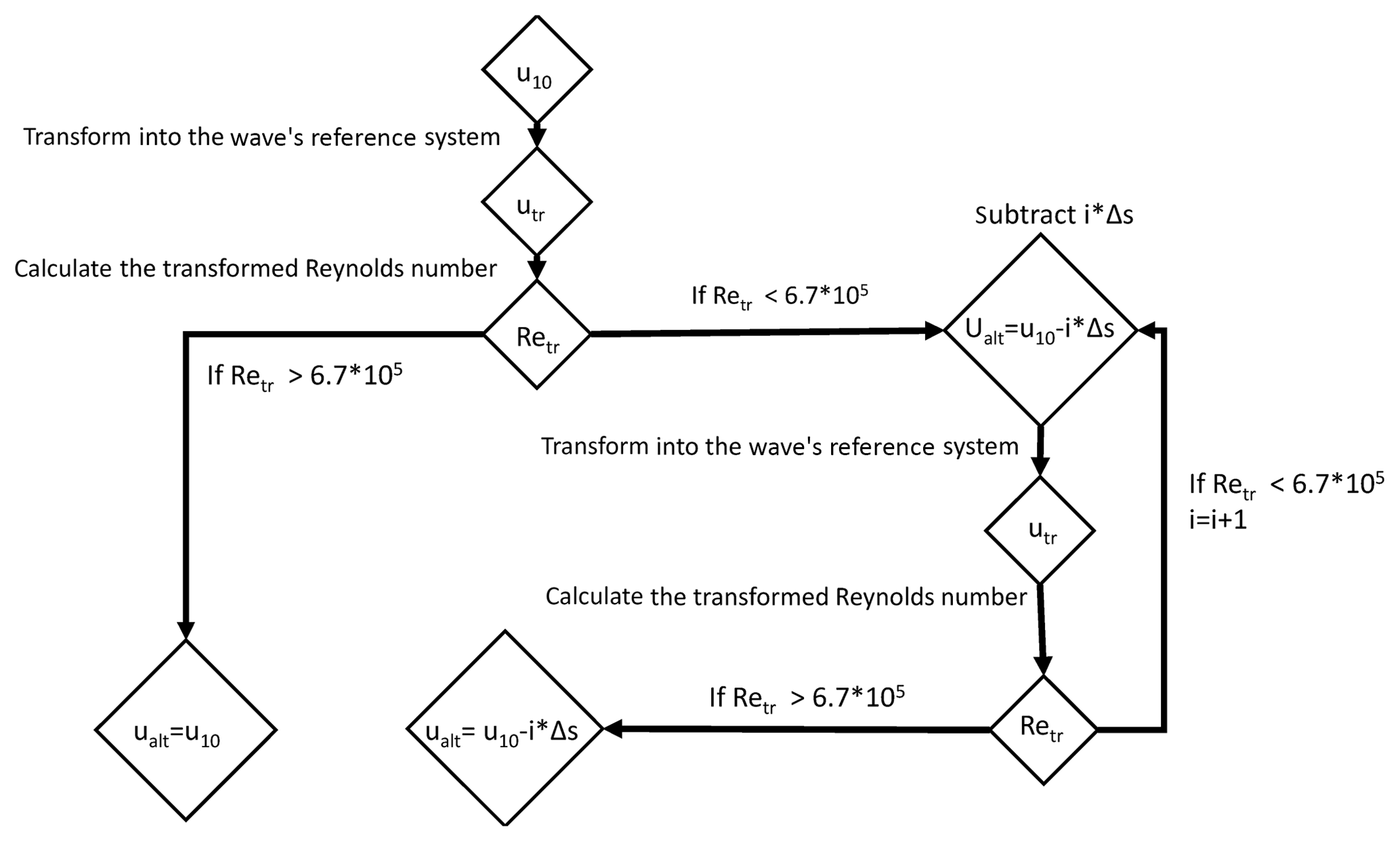
https://www.atmos-chem-phys.net/19/1819/2019/acp-19-1819-2019-f01

Figure 1Work flow of the gas transfer suppression model. In the case of suppressed gas transfer, the output is the adjusted wind speed u_alt, which can then be used in gas transfer parameterizations. The step size Δs can be adapted freely, but considerations of resolution and computing power have to be made. We set Δs=0.3 m s⁻¹ for this paper.

Download

Given a set wave field (constant H_s, wave direction and speed), if the relative wind speed in the reference system of the wave u_tr is high enough that $| R e_{tr} | > 6.96 \times 10^{5}$ , no suppression occurs. In the “unsuppressed” case, k can be estimated by common gas transfer parameterizations. If the wind speed u₁₀, in the earth's reference system, is getting close to the wave's phase speed, u_tr in the wave's reference system gets smaller and $| R e_{tr} |$ drops below the threshold; thus, flow separation happens and suppression occurs. We propose a stepwise (Δs) reduction of u₁₀ to calculate when the wind–wave system changes from the flow separation regime ( $| R e_{tr} | < 6.96 \times 10^{5}$ ) to a normal flow regime ( $| R e_{tr} | > 6.96 \times 10^{5}$ ). This can be used to estimate the magnitude of the suppression. We recalculate Re_tr with a lower $u_{alt} = u_{10} - i \cdot Δ s$ and iterate i=0, 1, 2, 3 … as long as Re_tr is below the threshold (flow separation). If Re_tr crosses to the non-suppressing regime, the iteration is stopped and the actual u_alt can be used as an alternative wind speed. The iteration steps are (1) calculate Re_tr using $u_{alt} = u_{10} - i \cdot Δ s$ and (2) determine if $| R e_{tr} | \leq 6.96 \times 10^{5}$ . (3) If yes, $i = i + 1$ and continue with step (1). If no, break the loop. The step size in this model was 0.3 m s⁻¹. We think this step size allows for a good balance between computing time and velocity resolution. The minimum velocity for u_alt is 0 m s⁻¹. Figure 1 shows a flowchart of the algorithm. This algorithm is applied to every box at every time step.

A change in the parameters of the wave field is, in our opinion, not feasible as the wave field is influenced to a certain extent by swell that is externally prescribed. Swell travels long distances and does not necessarily have a direct relation to the wind conditions at the location of the gas transfer and measurement. Therefore, we change the wind speed only.

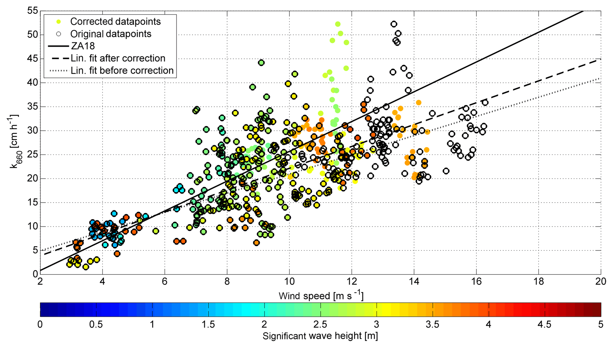
https://www.atmos-chem-phys.net/19/1819/2019/acp-19-1819-2019-f02

Figure 2Adjustments to the SO234-2/235 DMS k vs. u relationship. The datapoints with $| R e_{tr} | ≺ 6.96 \times 10^{5}$ were adjusted using the gas transfer suppression model. Black circles denote k values at the original wind speed u₁₀. Colored filled circles denote the k value at wind speed equals to u_alt. The color shows the significant wave height. If a datapoint has a concentric black and filled circle, it was not adjusted, as it was not subject to gas transfer suppression. The black solid line is the ZA18 parameterization. The dotted line is the linear fit to the datapoints before the adjustment; the dashed line is the linear fit after the adjustment.

Download

3.1 Gas transfer

The difference between u_alt and u₁₀ directly relates to the magnitude of gas transfer suppression. u_alt can be used in two ways: (1) u₁₀ can be directly replaced by u_alt. This is only possible for parameterizations with a negligible bubble contribution (like DMS), as we assume that the gas transfer suppression only affects k_o. As a result, one gets a k estimation using the lower wind speed u_alt. This is an estimate of the reduction of k by gas transfer suppression. (2) For parameterizations of rather insoluble gases, like CO₂, SF₆ and ³He, one needs to subtract Δk from the unsuppressed k parameterization. This adjustment is done by inserting u₁₀−u_alt into a k_o parameterization (Eq. 12) and subtracting Δk. In this paper, ZA18 from Zavarsky et al. (2018) is used as the parameterization of k_o. The magnitude of the gas transfer suppression is given by Eq. (12).

\begin{array}{l} Δ k & = k_{o} (u_{10}) - k_{o} (u_{alt}) = (3.1 \cdot u_{10} - 5.7) \\ (12) & - (3.1 \cdot u_{alt} - 5.7) = 3.1 \cdot (u_{10} - u_{alt}) \end{array}

For the global flux of DMS we use the bulk gas transfer formula (Eq. 1). The global DMS gas flux calculations are based on the following k parameterizations: ZA18 and the quadratic parameterization N00. For every grid box and every time step we calculate u_alt according to the description in Sect. 3. If u_alt is lower than u₁₀ from the global reanalysis, then gas transfer suppression occurs. Subsequently, u_alt together with Eq. (12) is used in the specific bulk gas transfer formulas (Eqs. 13–14). For ZA18, u_alt can be directly inserted into the ZA18 parameterization (Eq. 13). However, other parameterizations, e.g., N00, which are based on measurements with rather insoluble gases, have a significant bubble-mediated gas transfer contribution. As a consequence, we subtract the linearly dependent Δk using the ZA18 parameterization, to account for the gas transfer suppression in k_o (Eq. 14).

\begin{array}{l} F_{\lim, ZA 18} & = [k_{ZA 18} (u_{10}) - Δ k] \cdot Δ C \\ (13) & = (3.1 \cdot u_{alt} - 5.37) \cdot Δ C \end{array}

\begin{array}{l} F_{\lim, N 00 & other} & = [k_{N 00 & other} (u_{10}) - Δ k] \cdot Δ C \\ (14) & = [k_{N 00 & other} (u_{10}) - 3.1 \cdot (u_{10} - u_{alt})] \cdot Δ C \end{array}

Sea ice concentration from the ERA-Interim reanalysis was included as a linear factor in the calculation. A sea ice concentration of 90 %, for example, results in a 90 % reduction of the flux. Each time step (3 h) of the WWIII model provided a global grid of air–sea fluxes with and without gas transfer suppression. These single time steps were summed up to get a yearly flux result.

4 Results

We test the adjustment of u₁₀→u_alt with two data sets of DMS gas transfer velocities, Knorr11 (Bell et al., 2017) and SO234-2/235 (Zavarsky et al., 2018). Both data sets experienced gas transfer suppression at high wind speed. Using this proof of concept, we quantify the influence of gas transfer suppression on N00 and W14 and provide unsuppressed estimates. Finally, we apply the wind speed adjustment to global flux estimates of DMS. For CO₂, we estimate the magnitude of gas transfer suppression.

4.1 Adjustment of the interfacial gas transfer

Figures 2 and 3 show the unsuppressed DMS gas transfer velocities for the SO234-2/235 and the Knorr11 cruises. We shift the measured datapoints, which are gas transfer suppressed, along the x axis by replacing u₁₀ with u_alt. The shift along the x axis is equivalent to an addition of Δk, for a given k vs. u relationship, to balance gas transfer suppression (see Appendix). The black circles indicate the original data set at u₁₀. The colored circles are k values plotted at the adjusted wind speed u_alt. If a black circle and a colored circle are concentric, the datapoint was not suppressed and therefore no adjustment was applied. For comparison, the parameterization ZA18 is plotted in both figures. Both figures show the significant wave height with the color bar.

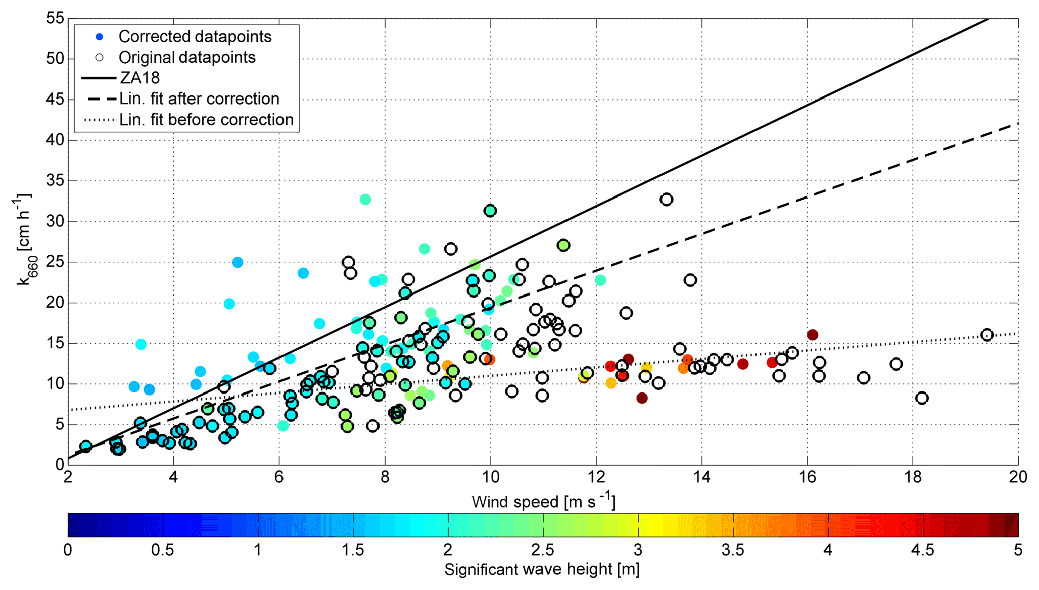
https://www.atmos-chem-phys.net/19/1819/2019/acp-19-1819-2019-f03

Figure 3Adjustments to the Knorr11 DMS k vs. u relationship. The datapoints with $| R e_{tr} | ≺ 6.96 \times 10^{5}$ were adjusted using the gas transfer suppression model. Black circles denote k values at the original wind speed u₁₀. Colored filled circles denote the k value at wind speed equal to u_alt. The color shows the significant wave height. If a datapoint has a concentric black and filled circle, it was not adjusted, as it was not subject to gas transfer suppression. The solid black line is the ZA18 parameterization. The dotted line is the linear fit to the datapoints before the adjustment; the dashed line is the linear fit after the adjustment.

Download

Figure 2 illustrates the linear fits to the data set before (dotted) and after (dashed) the adjustment. The suppressed datapoints from 14 to 16 m s⁻¹ moved closer to the linear fit after an adjustment with u_alt. The high gas transfer velocity values at around 13 m s⁻¹ and above 35 cm h⁻¹ were moved to 11 m⁻¹. This means a worsening of the k estimate by the linear fit. These datapoints have very low ΔC values (Zavarsky et al., 2018), therefore we expect a large scatter as a result from Eq. (2).

Table 1Mean differences between the reference fits (column one) and the adjusted and unadjusted k data sets. A negative value describes that the fit, on average, overestimates the actual measured data. The mean of the absolute value is presented in the last two columns.

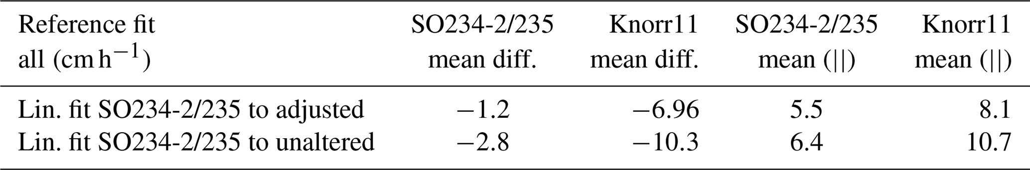
Download Print Version | Download XLSX

Table 2Linear fits to the adjusted and unadjusted data sets of Knorr11 and SO234-2/235. The error estimates correspond to a 95 % confidence interval.

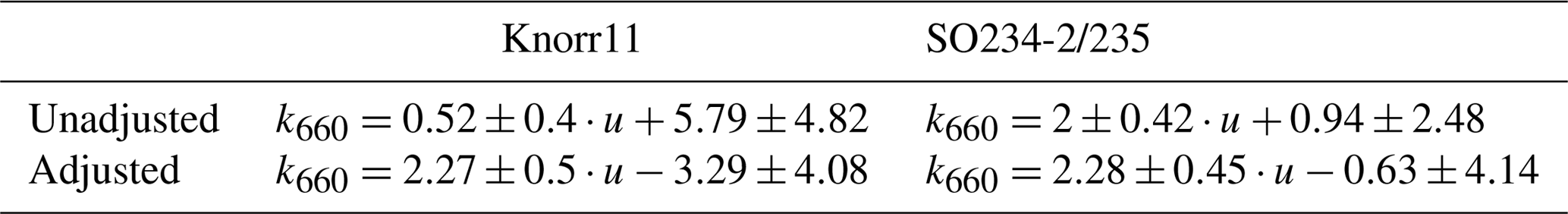
Download Print Version | Download XLSX

Figure 3 also shows an improvement of the linear fit estimates. The gas transfer suppressed datapoints were assigned the new wind speed u_alt, resulting in better agreement to ZA18. The change of the linear fit to the unsuppressed and suppressed data set can be seen in the dotted (before) and dashed (after) line. The adjusted datapoints at 12–16 m s⁻¹ are still, relative to the linear estimates, heavily gas transfer suppressed. A reason could be that the significant wave height of these points is larger than 3.5 m and they experienced high wind speed. A shielding of wind by the large wave or an influence of water droplets on the momentum transfer is suggested as another reason (Yang et al., 2016; Bell et al., 2013). In principle, we agree that these processes may be occurring, but only during exceptional cases of high winds and wave heights. The Reynolds gas transfer suppression (Zavarsky et al., 2018) occurs over a wider range of wind speeds and wave heights, but obviously does not capture all the flux suppression. Therefore, it appears that several processes, including shielding and influence of droplets, may be responsible for gas transfer suppression and they are not all considered in our model. This marks the upper boundary for environmental conditions for our model.

Table 1 shows the average offset between every datapoint and the linear fit ZA18. A reduction of the average offset can be seen for all data combinations. The last two columns of Table 1 show the mean absolute error. The absolute error also decreases with the application of our adjustments. The linear fits to the two data sets, before and after the adjustments, are given in Table 2.

The slopes for the two altered data sets show a good agreement. However, we do not account for the suppression entirely. The adjusted slopes are both in the range of the linear function ZA18 $k_{660} = 3.1 \pm 0.37 \cdot u_{10} - 5.37 \pm 2.35$ (Zavarsky et al., 2018), but the slopes barely overlap within the 95 % confidence interval.

4.2 Nightingale parameterization

The N00 parameterization is a quadratic wind-speed-dependent parameterization of k. It is widely used, especially for regional bulk CO₂ gas flux calculations as well as for DMS flux calculations in Lana et al. (2011). The parameterization is based on dual-tracer measurements in the water performed in the North Sea (Watson et al., 1991; Nightingale et al., 2000) as well as data from the Florida Strait (FS; Wanninkhof et al., 1997) and Georges Bank (GB; Wanninkhof, 1992).

We analyzed each individual measurement that was used in the parameterization to assess the amount of gas transfer suppressing instances that are within the N00 parameterization. The single measurements, which are used for fitting the quadratic function of the N00 parametrization, are shown together with N00 in Fig. 4a. As the measurement time of the dual-tracer technique is on the order of days, we interpolated the wind and wave data, obtained from the WWIII model for the specific time and location, to 1 h time steps and calculated the number of gas transfer suppressing and gas transfer non-suppressing instances. Fig. 4b shows the suppression index, which is the ratio of gas suppressing instances to the number of datapoints (x axis). The value 1 indicates that all of the interpolated 1 h steps were gas transfer suppressed. The y axis of Fig. 4 depicts the relation of the individual measurements to the N00 parameterization. A ratio (y axis) of 1 indicates that the measurement point is exactly the same as the N00 parameterization. A value of 1.1 would indicate that the value was 10 % higher than predicted by the N00 parameterization.

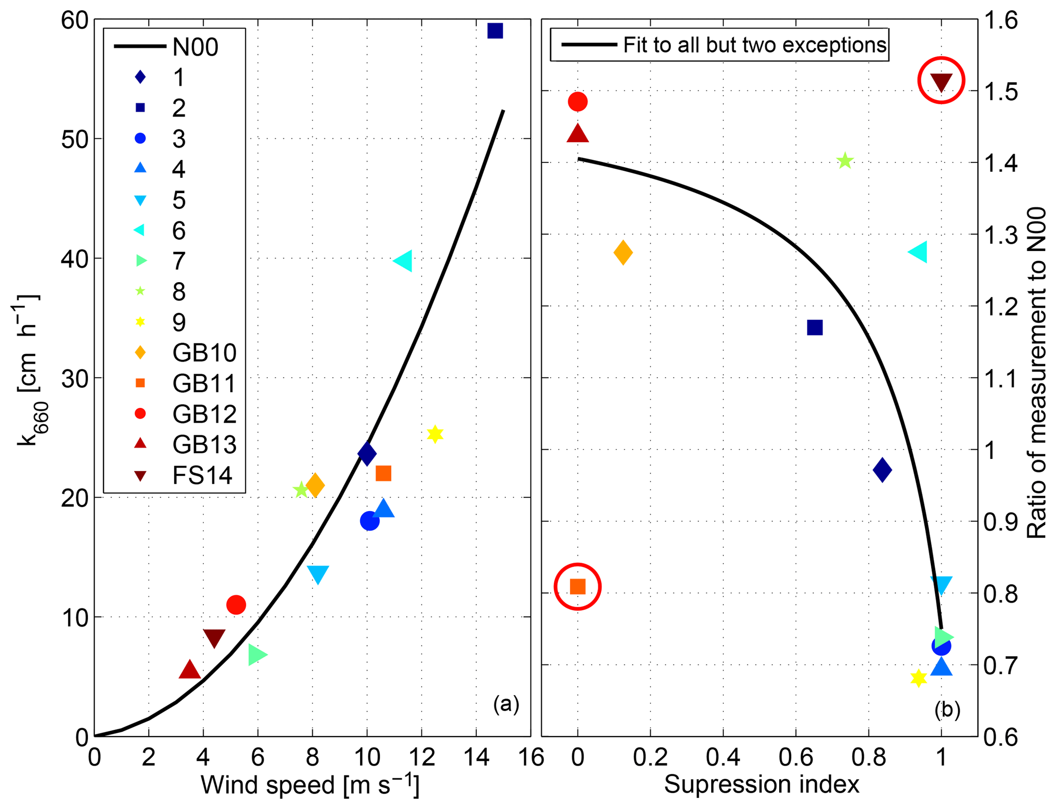
https://www.atmos-chem-phys.net/19/1819/2019/acp-19-1819-2019-f04

Figure 4Individual dual-tracer measurements that contribute to the N00 (solid line) parameterization (a). The relationship of the gas suppression ratio to the measurement and N00 ratio (b). The solid line in (b) is a fit to the suppression to measurement and N00 relationship. A higher suppression ratio indicates a longer influence of gas transfer suppression on the datapoint. The two red circles denote the outlier points that are discussed in the text. The solid black line is a fit using the function $y (x) = a_{1} + a_{2} \cdot \frac{1}{x - a_{3}}$ . The fit coefficients are a₁=1.52, a₂=0.14 and a₃=1.18.

Download

We expect a negative correlation between the suppression index and the relation of the individual measurement vs. the N00 parameterization. The higher the suppression index, the higher the gas transfer suppression and the lower the gas transfer velocity k with respect to the average parameterization. The correlation (Spearman's rank) is −0.43 with a significance level (p value) of 0.11. This is not significant. However, we must take a closer look at two specific points: (1) point 11, GB11 that shows low measurement percentage despite a low suppression index, and (2) point 14, FS14 that shows high measurement percentage despite a high suppression index. GB11 at the Georges Bank showed an average significant wave height of 3.5 m, with a maximum of 6 m and wind speed between 9 and 13 m s⁻¹. Transformed wind speeds u_tr are between 4 and 20 m s⁻¹. As already discussed in Sect. 4.1 using the Knorr11 data set, wave heights above 3.5 m could lead to gas transfer suppression without being captured by the Reynolds gas transfer suppression model (Zavarsky et al., 2018). High waves together with the strong winds could mark an upper limit of the gas transfer suppression model (Zavarsky et al., 2018). On the other hand, the FS14 datapoint showed an average wave height of 0.6 m and wind speed of 4.7 m s⁻¹. It is questionable if a flow separation and a substantial wind–wave interaction can be established at this small wave height. This could mark the lower boundary for the Reynolds gas transfer suppression model (Zavarsky et al., 2018). Taking out either one or both of these measurements (GB11 or FS14) changes the correlation (Spearman's rank) to −0.62 p=0.0233 (excluding GB11), −0.59 p=0.033 (excluding FS14) and −0.79 p=0.0025 (excluding GB11 and FS14). All three are significant. The solid black line in Fig. 4b is a fit to all points except GB11 and FS14, and based on Eq. (15).

\begin{matrix} (15) & y (x) = a_{1} + a_{2} \cdot \frac{1}{x - a_{3}} \end{matrix}

We choose this functional form and hypothesize that gas transfer suppression is not linear, but rather has a threshold (Zavarsky et al., 2018). This means that the influence of suppression on gas transfer is relatively low with a small suppression ratio, but increases strongly. The fit coefficients are a₁=1.52, a₂=0.14 and a₃=1.18.

Figure 5 shows the unsuppressed datapoints, according to the gas transfer suppression model (Sect. 3). We do not adjust the individual datapoints along the wind speed axis (x axis), as the parameterization has a significant bubble contribution, but add Δk (Eq. 12) to make up for the suppressed part of total k.

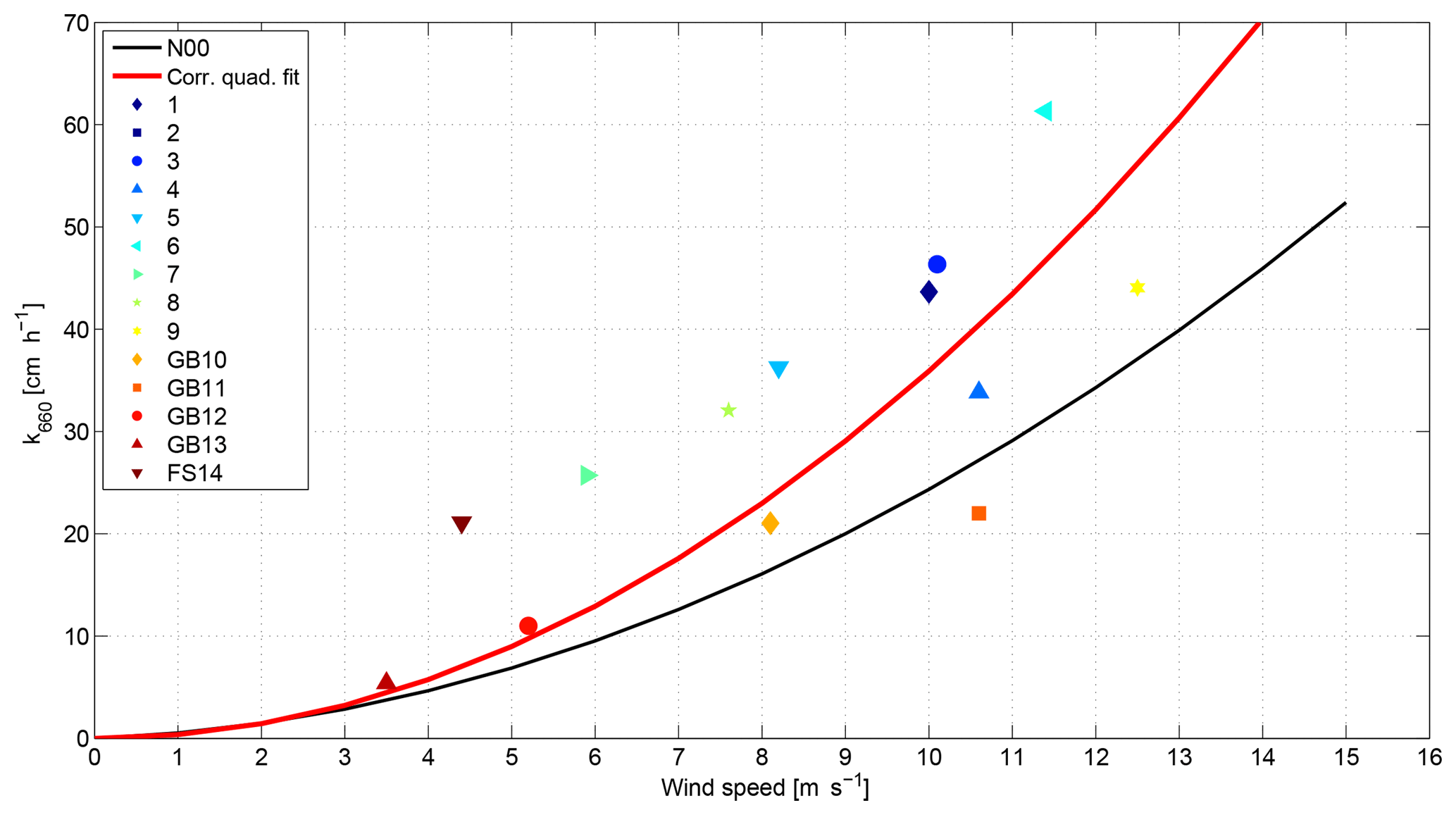
https://www.atmos-chem-phys.net/19/1819/2019/acp-19-1819-2019-f05

Figure 5Adjusted individual measurements, comprising the N00 parameterization, resulting from the algorithm described in Sect. 3. The difference between u_alt and the original u₁₀ was added to k using the linear parameterization ZA18, which accounts for the suppression of k_o due to wind–wave interaction. The solid black line is the original N00 parametrization. The red line is a new quadratic fit to the adjusted datapoints $k = 0.359 \cdot u^{2}$ .

Download

A new quadratic fit was applied to the adjusted datapoints (Eq. 16, Fig. 5).

\begin{matrix} (16) & k_{660} = 0.359 \cdot u^{2} \end{matrix}

On average, the new parameterization is 22 % higher than the original N00 parameterization. This increase is caused by the heavy gas transfer suppression of the individual measurements. As we believe that this suppression only affects the interfacial k_o gas exchange, it might not be easily visible (decreasing k vs. u relationship) in parameterizations based on dual-tracer gas transfer measurements, because of the potential of a large bubble influence.

The calculation of the unsuppressed N00 parameterization is an example application for this adjustment algorithm. We advise using the unsuppressed parameterization (N00 + 22 %) for flux calculations with very insoluble gases like SF₆or³He. We hypothesize that the original N00 contains a large bubble component, as it is based on SF₆ and ³He measurements, which is compensated by the gas transfer suppression. Therefore, the original N00 has been widely used for regional CO₂ gas flux calculations.

4.3 Wanninkhof parameterization

The W14 parameterization estimates the gas transfer velocity using the natural disequilibrium between ocean and atmosphere of ¹⁴C and the bomb ¹⁴C inventories. The total global gas transfer over several years is estimated by the influx of ¹⁴C in the ocean (Naegler, 2009) and the global wind speed distribution over several years. The parameterization from W14 is for winds averaged over several hours. The WWIII model wind data, used here, are 3 hourly and therefore in the proposed range (Wanninkhof, 2014). The W14 parameterization is given in Eq. (17).

\begin{matrix} (17) & k_{660, W 14} = 0.251 \cdot {(u_{10})}^{2} \end{matrix}

The interesting point about this parameterization is that it should already include a global average gas transfer suppressing factor. The parametrization is independent of local gas transfer suppression events. It utilizes a global, annual averaged, gas transfer velocity of ¹⁴C and relates it to remotely sensed wind speed. This means that the average gas transfer velocity has experienced the average global occurrence of gas transfer suppression and therefore is incorporated into the k vs. u parameterization.

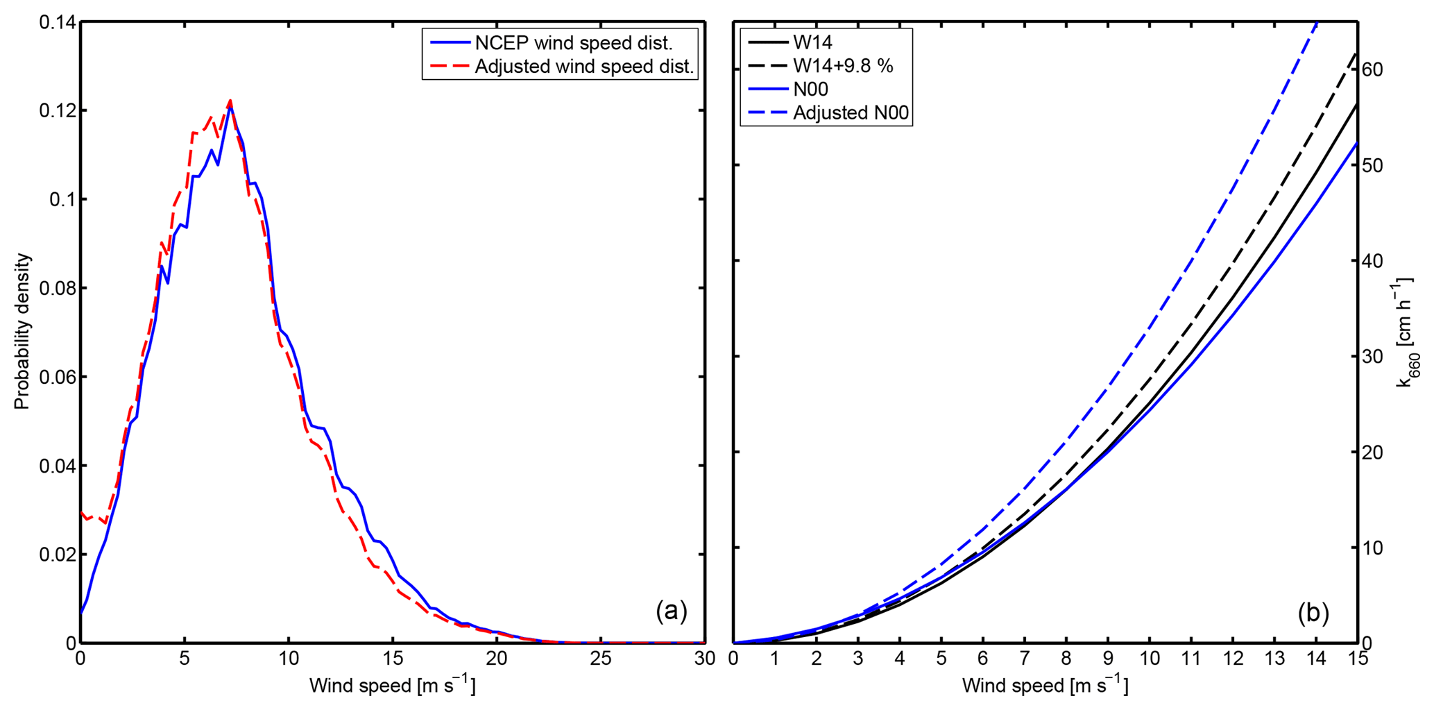
https://www.atmos-chem-phys.net/19/1819/2019/acp-19-1819-2019-f06

Figure 6Wind speed distributions for the year 2014 (a). The solid line is NCEP-derived wind speed distribution, the dashed line the wind speed distribution of the adjusted wind speed u_alt. Comparison of original and adjusted k vs. wind speed parameterizations (b).

Download

The quadratic coefficient, a, is calculated by dividing the averaged gas transfer velocity k_glob by u² and the wind distribution, distu, of u.

\begin{matrix} (18) & a = \frac{k_{glob}}{\sum u^{2} \cdot distu} \end{matrix}

The quadratic coefficient then defines the wind-speed-dependent gas transfer velocity k (Eq. 19).

\begin{matrix} (19) & k = a \cdot u^{2} \end{matrix}

The Fig. 6a shows the global wind speed distribution of the year 2014 taken from the WWIII model, which is based on the NCEP reanalysis. Additionally, we added the distribution taking our wind speed adjustment into account. At the occurrence of gas transfer suppression, we calculated u_alt as the representative wind speed for the unsuppressed transfer, as described in Sect. 3. The distribution of u_alt shifts higher wind speed (10–17 m s⁻¹) to lower wind speed regimes (0–7 m s⁻¹). This alters the coefficient for the quadratic wind speed parametrization. A global average gas transfer velocity of k_glob=16.5 cm h⁻¹ (Naegler, 2009) results in a coefficient a=0.2269, using the NCEP wind speed distribution. The value for a becomes 0.2439 with the u_alt distribution. This is a 9.85 % increase. Our calculated value of a=0.2269 differs from the W14 value of a=0.251 because we use a different wind speed distribution. The W14 uses a Rayleigh distribution with σ=5.83, our NCEP-derived σ=6.04 and the adjusted NCEP σ=5.78. This means that the W14 uses a wind speed distribution with a lower global average speed. However, for the estimation of a suppression effect we calculate the difference between using the NCEP wind speed and the adjusted wind speed distribution. For the calculation of a, we did not use a fitted Rayleigh function but the adjusted wind speed distribution from Fig. 6.

A comparison of W14, N00 and the unsuppressed parameterizations is shown in Fig. 6b. N00 shows the lowest relationship between u and k. W14 shows a parameterization with a global-averaged gas transfer suppression influence and is therefore slightly higher than N00. It appears that the gas transfer suppression is overcompensating the smaller bubble-mediated gas transfer of CO₂ (W14). The unsuppressed N00 is significantly higher than the W14 + 9.85 %. We hypothesize that this difference is based on the different bubble-mediated gas transfer of He, SF₆, and CO₂.

4.4 Global analysis

We used the native global grid (0.5^∘ × 0.5^∘) from the WWIII for the global analysis. The datapoints from the DMS and CO₂ climatologies as well as all auxiliary variables were interpolated to this grid.

Figure 7 shows the percentage of gas-transfer-suppressed datapoints with respect to the total datapoints for every month in the year 2014. The average yearly global percentage is 18.6 %. The minimum is 15 % in March and April and the maximum is 22 % in June–August. Coastal areas and marginal seas seem to be more influenced than open oceans. The reason could be that gas transfer suppression is likely to occur at developed wind seas when the wind speed is in the same direction and magnitude as the wave's phase speed. At coastal areas and marginal seas, the sea state is less influenced by swell and waves that were generated at a remote location. Landmasses block swell from the open ocean to marginal seas. The intra-annual variability of gas transfer suppression is shown in Fig. 8. Additionally, we plotted the occurrences split into ocean basins and northern and southern hemispheres. Two trends are visible. There is a higher percentage of gas transfer suppression in the Northern Hemisphere and, on the time axis, the peak is in the respective (boreal and austral) summer season. The Southern Hemisphere has a water-to-landmass ratio of 81 %, the Northern Hemisphere's ratio is 61 %. The area of free open water is therefore greater in the Southern Hemisphere. Gas transfer suppression is favored by fully developed seas without remote swell influence. In the Southern Hemisphere, the large open ocean areas, where swell can travel longer distances, provide an environment with less gas transfer suppression. The peak in summer and minimum in winter can be associated with the respective sea ice extent on the Northern Hemisphere and Southern Hemisphere. Figure 7 shows that seas, which are usually ice-covered in winter, have a high ratio of gas transfer suppression.

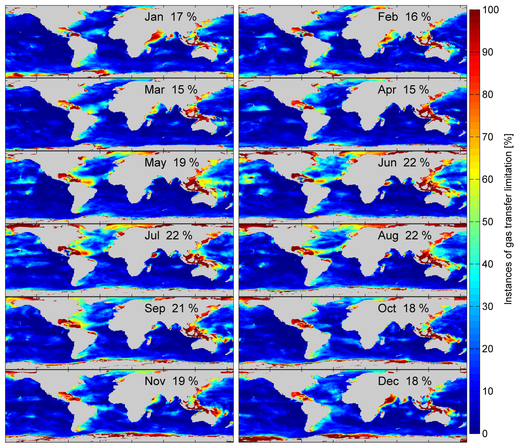
https://www.atmos-chem-phys.net/19/1819/2019/acp-19-1819-2019-f07

Figure 7The global probability of experiencing gas transfer suppression during the respective month (2014). The percentage is the number of gas transfer suppressed occurrences with respect to the total datapoints with a 3 h resolution.

Download

The global reduction of the CO₂ and DMS flux is calculated using Eqs. (13)–(14) and shown for every month in Figs. 9 and 10. These magnitudes represent the reduction of interfacial gas transfer due to gas transfer suppression. Most areas with a reduced influx of CO₂ into the ocean are in the Northern Hemisphere. The only reduced CO₂ influx areas of the Southern Hemisphere are in the South Atlantic and west of Australia and New Zealand. Significantly reduced CO₂ efflux areas are found in the northern tropical Atlantic, especially in the boreal summer months, the northern Indian Ocean and the Southern Ocean. The maximum monthly reduction of influx (oceanic uptake) is 18.7 mmol m⁻² day⁻¹. The maximum monthly reduction of efflux (oceanic outgassing) is 12.9 mmol m⁻² day⁻¹.

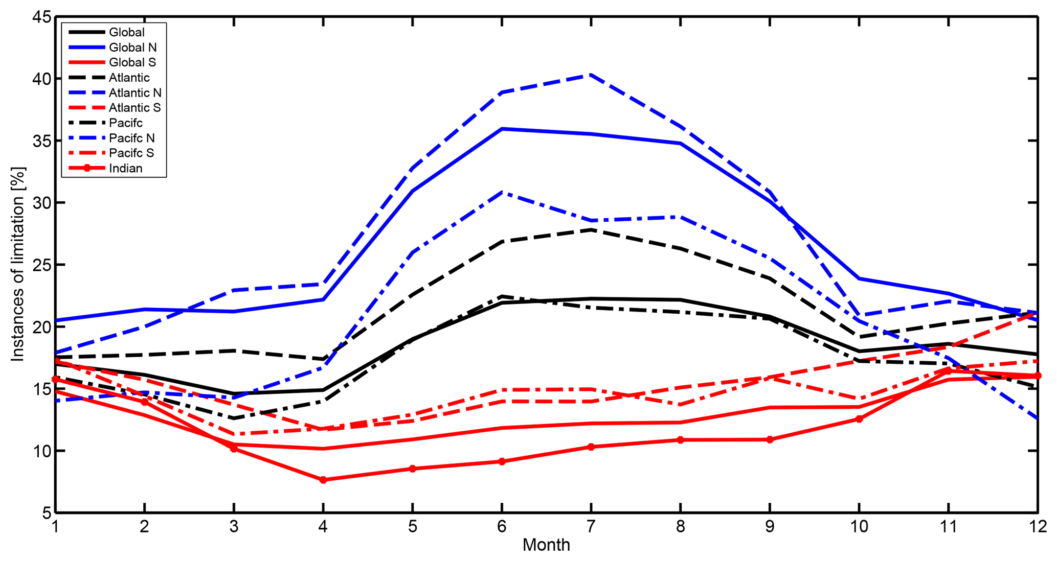
https://www.atmos-chem-phys.net/19/1819/2019/acp-19-1819-2019-f08

Figure 8The probability of experiencing gas transfer suppression during the respective month (2014) divided into ocean basins and hemispheres. The Southern Ocean was added to the southern part of the respective ocean basin. The percentage is the number of gas transfer suppressed instances with respect to the total datapoints with a 3 h resolution.

Download

https://www.atmos-chem-phys.net/19/1819/2019/acp-19-1819-2019-f09

Figure 9The absolute change of CO₂ gas transfer due to suppression for each month of 2014. Negative values (blue) denote areas where a flux into the ocean is reduced by the shown value. Positive values denote areas where flux out of the ocean is reduced by the shown value. The change is calculated using the bulk flux formula (Eq. 1) and Δk (Eq. 12).

Download

The absolute values of DMS flux reduction (Fig. 9), due to gas transfer suppression, coincide with the summer maximum of DMS concentration and therefore large air–sea fluxes (Lana et al., 2011; Simó and Pedrós-Alió, 1999). The northern Indian Ocean during boreal winter also shows a high level (10 µmol m² day⁻¹) of reduction. The highest water concentrations and fluxes in the Indian Ocean are found in boreal summer (Lana et al., 2011), which is less influenced by gas transfer suppression.

Lana et al. (2011)Lennartz et al. (2015)

Table 32014 DMS flux in teragrams. Re_tr indicates an application of the gas transfer suppression model. The last two rows are estimated from global climatologies.

Download Print Version | Download XLSX

https://www.atmos-chem-phys.net/19/1819/2019/acp-19-1819-2019-f10

Figure 10The absolute change of DMS gas transfer due to suppression for each month of 2014. The shown magnitudes denote the reduction by gas transfer suppression. The change is calculated using the bulk flux formula (Eq. 1) and Δk (Eq. 12).

Download

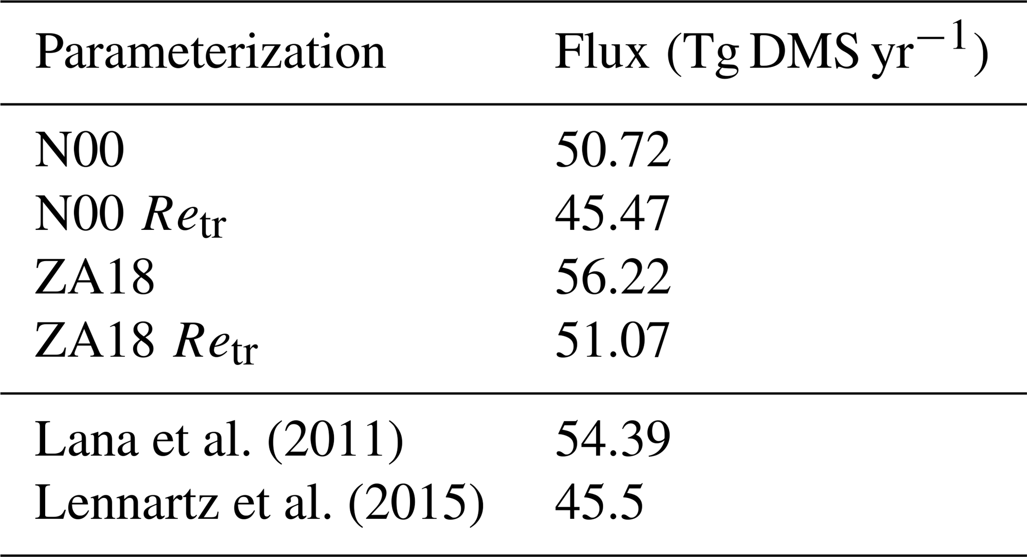
The DMS emissions from the ocean to the atmosphere are shown in Table 3. The calculated total emission from the original N00 parameterization is 50.72 Tg DMS yr⁻¹ for the year 2014. We use our estimations of u_alt and Eq. (14) to subtract gas transfer suppression from the original N00 parameterization. The resulting reduced total emission is 45.47 Tg DMS yr⁻¹, which is a reduction of 11 %. The linear parameterization ZA18 estimates an emission of 56.22 Tg DMS yr⁻¹. Using the gas transfer suppression algorithm and Eq. (13), the global amount is reduced to 51.07 Tg DMS yr⁻¹, which is a reduction of 11 %. Global estimates are 54.39 Tg DMS yr⁻¹ (Lana et al., 2011) and 45.5 Tg DMS yr⁻¹ (Lennartz et al., 2015). As stated above, a difference in wind speed or sea ice coverage could be the reason for the difference in the global emission estimated between the Lana climatology and our calculations with the N00 parameterization. Lennartz et al. (2015) use the water concentrations from the Lana climatology, but include air-side DMS concentrations, which reduces the flux by 17 %. We do not include air-side DMS concentrations but gas transfer suppression, which reduces the flux by 11 %. We can expect a reduction of 20 %–30 % when including both processes.

5 Conclusions

We provide a first approach to adjust k values for the gas transfer suppression due to wind–wave interaction (Zavarsky et al., 2018) and therefore to account for the effect of this suppression. Re_tr and the resulting alternative wind speed u_alt can be calculated from standard meteorological and oceanographic variables. Additionally, the condition (period, height, direction) of the ocean waves have to be known or retrieved from wave models. The calculation is iterative and can be easily implemented. The effect of this adjustment is shown with two data sets from the Knorr11 (Bell et al., 2017) and the SO234-2/235 cruises (Zavarsky et al., 2018). Both data sets show, after the adjustment, a better agreement with the linear ZA18 parameterizations (Tables 1 and 2), which only contains unsuppressed gas transfer velocity measurements from the SO 234-2/235 cruise. Generally, the adjustments may be only applied to the interfacial gas transfer velocity k_o.

We investigated the individual measurements leading to the N00 gas transfer parameterization for the influence of gas transfer suppression. We think that the overall parameterization is heavily influenced by gas transfer suppression, but the suppression is likely masked by bubble-mediated gas transfer, due to the solubility of the dual-tracer measurement gases. We show a significant negative correlation between the occurrence of gas transfer suppression and the ratio of the individual measurements to the N00 parameterization. We applied an adjustment due to gas transfer suppression and fitted a new quadratic function to the adjusted data set. The new parameterization is on average 22 % higher than the original N00 parameterization. This leads to the conclusion that gas transfer suppression influences gas transfer parameterizations, even if it is not directly visible, via a smaller slope. Asher and Wanninkhof (1998) state that SF₆∕³He gas transfer measurements could lead to a 23 % overestimation of CO₂ gas transfer velocities. After adjusting of N00 for gas transfer suppression, the difference between gas transfer velocities of the original N00 and the adjusted version closely matches this estimation.

For the W14 parameterization we used a global wind speed climatology for the year 2014 and applied the gas transfer suppression model u₁₀→u_alt. Using the distribution function of u_alt we calculated an unsuppressed gas transfer parameterization. The coefficient of the unsuppressed parameterization is 9.85 % higher than the original one. W14 already includes the global average of gas transfer suppression. Therefore the increase, due to the adjustment, is expected to be less than the one for N00, which is strongly suppressed. The original N00 is lower than W14, but after adjustment N00 is larger than the unsuppressed W14, which is expected due to the larger bubble-mediated gas transfer of He and SF₆ over CO₂.

We think that gas transfer suppression has a global influence on air–sea gas exchange of 10 %–11 %. These numbers are supported by the adjustment of the W14 parametrization as well as a global DMS gas transfer calculation. Local conditions may lead to much higher influences. Gas transfer velocity parameterizations from regional data sets might be heavily influenced by gas transfer suppression. We have shown this for the N00 parameterization. This should be considered with their use.

Using the Re_tr parameter, one can evaluate if a flux measurement or flux calculation is influenced by gas transfer suppression. For unsuppressed conditions and rather soluble gases, such as DMS, we recommend the use of a linear parameterization (e.g., ZA18). For gases with a similar solubility as CO₂, we recommend the use of the adjusted W14 + 9.85 % parameterization. The adjusted N00 (N00 + 22 %) parameterization is recommended for very insoluble gases. In case of gas transfer suppression, we recommend the previous parameterizations together with our iterative approach to adjust u to u_alt (Fig. 1) with the use of Eqs. (13)–(14). For global calculations, we recommend the use of the Wanninkhof parameterizations W14 (Wanninkhof, 2014), as it already has an average global gas transfer suppression included.

Data availability

The wave data are available at the website of the NOAA Environmental Modeling Center. The ERA-Interim data are available at the website of the ECMWF. The data are stored at the data portal of GEOMAR Kiel.

Appendix A: Directional dependencies

Figure A1 shows the shape of the wave (half sphere) as experienced by the wind flowing over it with a certain angle θ. The larger θ, the more streamlined the wave (half sphere). The more streamlined the wave, the more difficult it is to generate turbulence; this counteracts the flow detachment and as a consequence gas transfer suppression occurs.

Wind at an angle of θ=90^∘ does not experience a wave crest or trough, but rather an along-wind corrugated surface. In this case there should be no gas transfer suppression. Zavarsky et al. (2018) predict a unsuppressed condition around Re_tr=0, which coincides with θ≈90^∘ or u_tr→0. Both conditions rarely occur and must be investigated in the future.

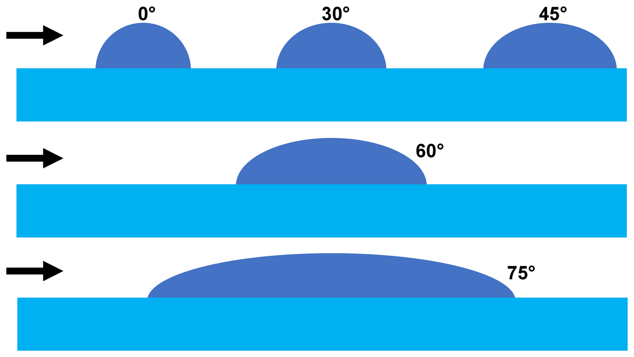
https://www.atmos-chem-phys.net/19/1819/2019/acp-19-1819-2019-f11

Figure A1The streamlined shape of a wave (cylindrical half sphere) that experiences wind flowing over it from various angles θ.

Download

Adjustment of wind speed or adjustment of k

A shift on the x axis from u₁₀ to u_alt is equivalent to an increase in k by Δk, when related to a linear relationship. We use the ZA18 parameterization as a reference (Eq. 12), which is a linear relationship describing k_o, as gas transfer suppression only affects interfacial gas transfer. Figure B1 illustrates the two different possibilities of adjusting suppressed gas transfer values.

https://www.atmos-chem-phys.net/19/1819/2019/acp-19-1819-2019-f12

Figure B1Illustration of the gas transfer suppression adjustments either along the wind speed or gas transfer velocity axis.

Download

The adjustments of the two DMS data sets (SO234-2/235 and Knorr11) are done by shifting u₁₀ along the x axis to u_alt. We want to test whether u₁₀ can be directly replaced by u_alt for k_o parameterizations. Gas transfer suppression adjustments for bubble-influenced parameterizations are done by adding Δk, which is directly related to the difference $Δ u = u_{10} - u_{alt}$ .

Author contributions

AZ developed the model. AZ and CAM provided and collected the data. AZ prepared the manuscript with contributions from CAM.

Competing interests

The authors declare that they have no conflict of interest.

Acknowledgements

The authors thank Kirstin Krüger, the chief scientist of the R/V Sonne cruise (SO234-2/235), as well as the captain and crew. We thank the Environmental Modeling Center at the NOAA/National Weather Service for providing the WAVEWATCH III^® data. We thank the European Centre for Medium-Range Weather Forecasts for providing the ERA-Interim data. This work was carried out under the Helmholtz Young Investigator Group of Christa A. Marandino, TRASE-EC (VH-NG-819), from the Helmholtz Association. The cruise 234-2/235 was financed by the BMBF, 03G0235A.

Edited by: Martin Heimann
Reviewed by: Christopher Fairall and Mingxi Yang

References

Asher, W. E. and Wanninkhof, R.: The effect of bubble-mediated gas transfer on purposeful dual-gaseous tracer experiments, J. Geophys. Res.-Oceans, 103, 10555–10560, https://doi.org/10.1029/98jc00245,1998. a

Bell, T. G., De Bruyn, W., Miller, S. D., Ward, B., Christensen, K. H., and Saltzman, E. S.: Air-sea dimethylsulfide (DMS) gas transfer in the North Atlantic: evidence for limited interfacial gas exchange at high wind speed, Atmos. Chem. Phys., 13, 11073–11087, https://doi.org/10.5194/acp-13-11073-2013, 2013. a, b

Bell, T. G., De Bruyn, W., Marandino, C. A., Miller, S. D., Law, C. S., Smith, M. J., and Saltzman, E. S.: Dimethylsulfide gas transfer coefficients from algal blooms in the Southern Ocean, Atmos. Chem. Phys., 15, 1783–1794, https://doi.org/10.5194/acp-15-1783-2015, 2015. a

Bell, T. G., Landwehr, S., Miller, S. D., de Bruyn, W. J., Callaghan, A. H., Scanlon, B., Ward, B., Yang, M., and Saltzman, E. S.: Estimation of bubble-mediated air–sea gas exchange from concurrent DMS and CO₂ transfer velocities at intermediate-high wind speeds, Atmos. Chem. Phys., 17, 9019–9033, https://doi.org/10.5194/acp-17-9019-2017, 2017. a, b

Blomquist, B. W., Brumer, S. E., Fairall, C. W., Huebert, B. J., Zappa, C. J., Brooks, I. M., Yang, M., Bariteau, L., Prytherch, J., Hare, J. E., Czerski, H., Matei, A., and Pascal, R. W.: Wind Speed and Sea State Dependencies of Air-Sea Gas Transfer: Results From the High Wind Speed Gas Exchange Study (HiWinGS), J. Geophys. Res.-Oceans, 122, 8034–8062, https://doi.org/10.1002/2017JC013181, 2017. a

Dee, D. P., Uppala, S. M., Simmons, A. J., Berrisford, P., Poli, P., Kobayashi, S., Andrae, U., Balmaseda, M. A., Balsamo, G., Bauer, P., Bechtold, P., Beljaars, A. C. M., van de Berg, L., Bidlot, J., Bormann, N., Delsol, C., Dragani, R., Fuentes, M., Geer, A. J., Haimberger, L., Healy, S. B., Hersbach, H., Holm, E. V., Isaksen, L., Kållberg, P., Köhler, M., Matricardi, M., McNally, A. P., Monge-Sanz, B. M., Morcrette, J. J., Park, B. K., Peubey, C., de Rosnay, P., Tavolato, C., Thepaut, J. N., and Vitart, F.: The ERA-Interim reanalysis: configuration and performance of the data assimilation system, Q. J. Roy. Meteorol. Soc., 137, 553–597, https://doi.org/10.1002/qj.828, 2011. a

Hanley, K. E., Belcher, S. E., and Sullivan, P. P.: A Global Climatology of Wind-Wave Interaction, J. Phys. Oceanogr., 40, 1263–1282, https://doi.org/10.1175/2010JPO4377.1, 2010. a

Komori, S., McGillis, W., and Kurose, R.: Gas Transfer at Water Surfaces, 2010, Kyoto University, available at: http://hdl.handle.net/2433/156156 (last access: 5 January 2018), 2011. a

Lana, A., Bell, T. G., Simo, R., Vallina, S. M., Ballabrera-Poy, J., Kettle, A. J., Dachs, J., Bopp, L., Saltzman, E. S., Stefels, J., Johnson, J. E., and Liss, P. .: An updated climatology of surface dimethlysulfide concentrations and emission fluxes in the global ocean, Global Biogeochem. Cy., 25, GB1004, https://doi.org/10.1029/2010GB003850, 2011. a, b, c, d, e, f

Lennartz, S. T., Krysztofiak, G., Marandino, C. A., Sinnhuber, B.-M., Tegtmeier, S., Ziska, F., Hossaini, R., Krüger, K., Montzka, S. A., Atlas, E., Oram, D. E., Keber, T., Bönisch, H., and Quack, B.: Modelling marine emissions and atmospheric distributions of halocarbons and dimethyl sulfide: the influence of prescribed water concentration vs. prescribed emissions, Atmos. Chem. Phys., 15, 11753–11772, https://doi.org/10.5194/acp-15-11753-2015, 2015. a, b, c, d

Naegler, T.: Reconciliation of excess ¹⁴C-constrained global CO₂ piston velocity estimates, Tellus B, 61, 372–384, https://doi.org/10.1111/j.1600-0889.2008.00408.x, 2009. a, b

Nightingale, P. D., Malin, G., Law, C. S., Watson, A. J., Liss, P. S., Liddicoat, M. I., Boutin, J., and Upstill-Goddard, R. C.: In situ evaluation of air-sea gas exchange parameterizations using novel conservative and volatile tracers, Global Biogeochem. Cy., 14, 373–387, https://doi.org/10.1029/1999GB900091, 2000. a, b, c

Simó, R. and Pedrós-Alió, C.: Role of vertical mixing in controlling the oceanic production of dimethyl sulphide, Nature, 402, 396–399, https://doi.org/10.1038/46516, 1999. a

Singh, S. P. and Mittal, S.: Flow past a cylinder: shear layer instability and drag crisis, Int. J. Numer. Meth. Fluids, 47, 75–98, https://doi.org/10.1002/fld.807, 2004. a

Takahashi, T., Sutherland, S. C., Wanninkhof, R., Sweeney, C., Feely, R. A., Chipman, D. W., Hales, B., Friederich, G., Chavez, F., Sabine, C., Watson, A., Bakker, D. C., Schuster, U., Metzl, N., Yoshikawa-Inoue, H., Ishii, M., Midorikawa, T., Nojiri, Y., Körtzinger, A., Steinhoff, T., Hoppema, M., Olafsson, J., Arnarson, T. S., Tilbrook, B., Johannessen, T., Olsen, A., Bellerby, R., Wong, C., Delille, B., Bates, N., and de Baar, H. J.: Climatological mean and decadal change in surface ocean pCO₂, and net sea–air CO₂ flux over the global oceans, Deep-Sea Res. Pt. II, 56, 554–577, https://doi.org/10.1016/j.dsr2.2008.12.009, 2009. a, b

Tolman, H. L.: User manual and system documentation of WAVEWATCH-III version 1.15, NOAA/NWS/NCEP/OMB Technical Note 151, US Department of Commerce, National Oceanic and Atmospheric Administration, National Weather Service, National Centersfor Environmental Prediction, Camp Springs, 97 pp., 1997. a

Tolman, H. L.: User manual and system documentation of WAVEWATCH-III version 1.18, NOAA/NWS/NCEP/OMB Technical Note 166, US Department of Commerce, National Oceanic and Atmospheric Administration, National Weather Service, National Centersfor Environmental Prediction, Camp Springs, 110 pp., 1999. a

Tolman, H. L.: User manual and system documentation of WAVEWATCH III TM version 3.14, NOAA/NWS/NCEP/MMAB Technical Note 276, US Department of Commerce, National Oceanic and Atmospheric Administration, National Weather Service, National Centersfor Environmental Prediction, Camp Springs, 220 pp., 2009. a

Wanninkhof, R.: Relationship between wind speed and gas exchange over the ocean, J. Geophys. Res.-Oceans, 97, 7373–7382, https://doi.org/10.1029/92JC00188, 1992. a, b, c

Wanninkhof, R.: Relationship between wind speed and gas exchange over the ocean revisited, Limnol. Oceanogr.: Methods, 12, 351–362, https://doi.org/10.4319/lom.2014.12.351, 2014. a, b, c, d

Wanninkhof, R., Hitchcock, G., Wiseman, W. J., Vargo, G., Ortner, P. B., Asher, W., Ho, D. T., Schlosser, P., Dickson, M.-L., Masserini, R., Fanning, K., and Zhang, J.-Z.: Gas exchange, dispersion, and biological productivity on the West Florida Shelf: Results from a Lagrangian Tracer Study, Geophys. Res. Lett., 24, 1767–1770, https://doi.org/10.1029/97GL01757, 1997. a

Watson, A. J., Upstill-Goddard, R. C., and Liss, P. S.: Air-sea gas exchange in rough and stormy seas measured by a dual-tracer technique, Nature, 349, 145–147, https://doi.org/10.1038/349145a0, 1991. a

White, F.: Viscous Fluid Flow, McGraw-Hill series in mechanical engineering, McGraw-Hill, available at: https://books.google.de/books?id=G6IeAQAAIAAJ (last access: February 2019), 1991. a, b

Yang, M., Bell, T. G., Blomquist, B. W., Fairall, C. W., Brooks, I. M., and Nightingale, P. D.: Air-sea transfer of gas phase controlled compounds, IOP Conf. Ser.: Earth Environ. Sci., 35, 012011, https://doi.org/10.1088/1755-1315/35/1/012011, 2016. a, b

Zavarsky, A., Goddijn-Murphy, L., Steinhoff, T., and Marandino, C. A.: Bubble mediated gas transfer and gas transfer suppression of DMS and CO₂, J. Geophys. Res.-Atmos., 123, 6624–6647, https://doi.org/10.1029/2017jd028071, 2018. a, b, c, d, e, f, g, h, i, j, k, l, m, n, o, p

Articles

Short summary

Wind–wave interaction can suppress gas transfer between the atmosphere and the ocean. Using a global wave model we investigate the impact of this interaction on the global gas transfer of CO₂ and DMS. We also investigate the impact on of gas transfer limitation on two commonly used gas transfer velocity parameterizations.

The influence of transformed Reynolds number suppression on gas transfer parameterizations and global DMS and CO2 fluxes

2.1 WAVEWATCH III® (WWIII)

2.2 Auxiliary variables

2.3 Kinematic viscosity

2.4 Transformed Reynolds number

3.1 Gas transfer

4.1 Adjustment of the interfacial gas transfer

4.2 Nightingale parameterization

4.3 Wanninkhof parameterization

4.4 Global analysis

The influence of transformed Reynolds number suppression on gas transfer parameterizations and global DMS and CO₂ fluxes

2.1 WAVEWATCH III^® (WWIII)