the Creative Commons Attribution 4.0 License.
the Creative Commons Attribution 4.0 License.
 | 08 Feb 2019
A top-down assessment using OMI NO2 suggests an underestimate in the NOx emissions inventory in Seoul, South Korea, during KORUS-AQ
Pablo E. Saide
Lok N. Lamsal
Benjamin de Foy
Zifeng Lu
Jung-Hun Woo
Younha Kim
Jinseok Kim
Gregory Carmichael
David G. Streets
In this work, we investigate the NOx emissions inventory in Seoul, South Korea, using a regional ozone monitoring instrument (OMI) NO2 product derived from the standard NASA product. We first develop a regional OMI NO2 product by recalculating the air mass factors using a high-resolution (4 km × 4 km) WRF-Chem model simulation, which better captures the NO2 profile shapes in urban regions. We then apply a model-derived spatial averaging kernel to further downscale the retrieval and account for the subpixel variability. These two modifications yield OMI NO2 values in the regional product that are 1.37 times larger in the Seoul metropolitan region and >2 times larger near substantial point sources. These two modifications also yield an OMI NO2 product that is in better agreement with the Pandora NO2 spectrometer measurements acquired during the South Korea–United States Air Quality (KORUS-AQ) field campaign. NOx emissions are then derived for the Seoul metropolitan area during the KORUS-AQ field campaign using a top-down approach with the standard and regional NASA OMI NO2 products. We first apply the top-down approach to a model simulation to ensure that the method is appropriate: the WRF-Chem simulation utilizing the bottom-up emissions inventory yields a NOx emissions rate of 227±94 kt yr−1, while the bottom-up inventory itself within a 40 km radius of Seoul yields a NOx emissions rate of 198 kt yr−1. Using the top-down approach on the regional OMI NO2 product, we derive the NOx emissions rate from Seoul to be 484±201 kt yr−1, and a 353±146 kt yr−1 NOx emissions rate using the standard NASA OMI NO2 product. This suggests an underestimate of 53 % and 36 % in the bottom-up inventory using the regional and standard NASA OMI NO2 products respectively. To supplement this finding, we compare the NO2 and NOy simulated by WRF-Chem to observations of the same quantity acquired by aircraft and find a model underestimate. When NOx emissions in the WRF-Chem model are increased by a factor of 2.13 in the Seoul metropolitan area, there is better agreement with KORUS-AQ aircraft observations and the recalculated OMI NO2 tropospheric columns. Finally, we show that by using a WRF-Chem simulation with an updated emissions inventory to recalculate the air mass factor (AMF), there are small differences (∼8 %) in OMI NO2 compared to using the original WRF-Chem simulation to derive the AMF. This suggests that changes in model resolution have a larger effect on the AMF calculation than modifications to the South Korean emissions inventory. Although the current work is focused on South Korea using OMI, the methodology developed in this work can be applied to other world regions using TROPOMI and future satellite datasets (e.g., GEMS and TEMPO) to produce high-quality region-specific top-down NOx emissions estimates.


Nitrogen oxides (NOx≡NO+NO2) are a group of reactive trace gases that are toxic to human health and can be converted in the atmosphere into other noxious chemical species. In the presence of abundant volatile organic compounds (VOCs) and strong sunlight, NOx can participate in a series of chemical reactions to generate a net accumulation of O3, another toxic air pollutant with a longer atmospheric lifetime. NOx also participates in a series of reactions to create HNO3, a key contributor to acid rain, and particulate nitrate (), a component of fine particulate matter (PM2.5), an additional health hazard. There are some natural emissions of NOx (e.g., lightning), but the majority of the NOx emissions are from anthropogenic sources (van Vuuren et al., 2011).
There is a rich legacy of NO2 measurements by remote sensing instruments (Burrows et al., 1999). One of these instruments is the Dutch–Finnish ozone monitoring instrument (OMI), which measures the absorption of solar backscatter in the UV–visible spectral range. NO2 can be observed from space because it has strong absorption features within the 400–465 nm wavelength region (Vandaele et al., 1998). By comparing observed spectra with a reference spectrum, the amount of NO2 in the atmosphere between the instrument in low-Earth orbit and the surface can be derived; this technique is called differential optical absorption spectroscopy (DOAS) (Platt, 1994).
Tropospheric NO2 column contents from OMI have been used to estimate NOx emissions from various areas around the globe (Streets et al., 2013; Miyazaki et al., 2017) including North America (Boersma et al., 2008; Lu et al., 2015), Asia (Zhang et al., 2008; Han et al., 2015; Kuhlmann et al., 2015; Liu et al., 2017), the Middle East (Beirle et al., 2011), and Europe (Huijnen et al., 2010; Curier et al., 2014). It has also been used to produce and validate NOx emissions estimates from sources such as soil (Hudman et al., 2010; Vinken et al., 2014a; Rasool et al., 2016), lightning (Allen et al., 2012; Liaskos et al., 2015; Pickering et al., 2016; Nault et al., 2017), power plants (de Foy et al., 2015), aircraft (Pujadas et al., 2011), marine vessels (Vinken et al., 2014b; Boersma et al., 2015), and urban centers (Lu et al., 2015; Canty et al., 2015; Souri et al., 2016).
With a pixel resolution varying from 13 km × 24 km to 26 km × 128 km, the OMI sensor was developed for global- to regional-scale studies rather than for individual urban areas. Even at the highest spatial resolution of 13 km × 24 km, the sensor has difficulty observing the fine structure of NO2 plumes at or near the surface (e.g., highways, power plants, factories) (Chen et al., 2009; Ma et al., 2013; Flynn et al., 2014), which are often less than 10 km in width (Heue et al., 2008). This can lead to a spatial averaging of pollution (Hilboll et al., 2013). A temporary remedy, until higher spatial resolution satellite instruments are operational, is to use a regional air quality simulation to estimate the subpixel variability of OMI pixels. Kim et al. (2016) utilize the spatial variability in a regional air quality model to spatially downscale OMI NO2 measurements using a spatial averaging kernel. The spatial averaging kernel technique has been shown to increase the OMI NO2 signal within urban areas, which is in better agreement with observations in these regions (Goldberg et al., 2017).
Furthermore, the air mass factor and surface reflectance used in obtaining the global OMI NO2 retrievals are at a coarse spatial resolution (Lorente et al., 2017; Kleipool et al., 2008). While appropriate for a global operational retrieval, this is known to cause an underestimate in the OMI NO2 signal in urban regions (Russell et al., 2011). The air mass factors in the operational OMI NO2 retrieval are calculated using NO2 profile shapes that are provided at a 1.25∘ × 1∘ spatial resolution in the NASA product (Krotkov et al., 2017) and 2∘ × 3∘ spatial resolution in the DOMINO product (Boersma et al., 2011). Developers of the NASA product provide scattering weights and additional auxiliary information so that users can develop their own tropospheric vertical column product a posteriori (Lamsal et al., 2015). Several users have recalculated the air mass factor using a regional air quality model (Russell et al., 2011; Kuhlmann et al., 2015; Lin et al., 2015; Goldberg et al., 2017; Laughner et al., 2019), which can better capture the NO2 profile shapes in urban regions. Other techniques to improve the air mass factor involve correcting for the surface pressure in mountainous terrain (Zhou et al., 2009) and accounting for small-scale heterogeneities in surface reflectance (Zhou et al., 2010; Vasilkov et al., 2017). These a posteriori products have better agreement with ground-based spectrometers measuring tropospheric vertical column contents (Goldberg et al., 2017). When available, observations from aircraft can constrain the NO2 profile shapes used in the air mass factor calculation (Goldberg et al., 2017).
In this paper, we apply both techniques (the spatial averaging kernel and an air mass factor adjustment) to develop a regional OMI NO2 product for South Korea. We then use the regional product with only the air mass factor adjustment to derive NOx emissions estimates for the Seoul metropolitan area using a statistical fit to an exponentially modified Gaussian (EMG) function (Beirle et al., 2011; Valin et al., 2013; de Foy et al., 2014; Lu et al., 2015); the methodology is described in depth in Sect. 2.5.
2.1 OMI NO2
OMI has been operational on NASA's Earth Observing System Aura satellite since October 2004 (Levelt et al., 2006). The satellite follows a sun-synchronous, low-Earth (705 km) orbit with an Equator overpass time of approximately 13:45 local time. OMI measures total column amounts in a 2600 km swath divided into 60 unequal area “fields of view”, or pixels. At nadir (center of the swath), pixel size is 13 km × 24 km, but at the swath edges, pixels can be as large as 26 km × 128 km. In a single orbit, OMI measures approximately 1650 swaths and achieves daily global coverage over 14–15 orbits (99 min per orbit). Since June 2007, there has been a partial blockage of the detector's full field of view, which has limited the number of valid measurements by blocking consistent rows of data; this is known in the community as the row anomaly (Dobber et al., 2008): http://projects.knmi.nl/omi/research/product/rowanomaly-background.php (last access: 1 February 2019).
OMI measures radiance data between the instrument's detector and the Earth's surface. Comparison of these measurements with a reference spectrum (i.e., DOAS technique) enables the calculation of the total slant column density (SCD), which represents an integrated trace gas abundance from the sun to the surface and back to the instrument's detector, passing through the atmosphere twice. For tropospheric air quality studies, vertical column density (VCD) data are more relevant. This is done by subtracting the stratospheric slant column from the total (tropospheric + stratospheric) slant column and dividing by the tropospheric air mass factor (AMF), which is defined as the ratio of the SCD to the VCD, as shown in Eq. (1):
The tropospheric AMF has been derived to be a function of the optical atmospheric and surface properties (viewing and solar angles, surface reflectivity, cloud radiance fraction, and cloud height) and a priori profile shape (Palmer et al., 2001; Martin et al., 2002) and can be calculated as follows (Lamsal et al., 2014) in Eq. (2):
where x is the partial column. The optical atmospheric and surface properties in the NASA retrieval are characterized by the scattering weight, which is calculated by the TOMRAD forward radiative transfer model. The scattering weights are first output as a lookup table and then adjusted to real time depending on observed viewing angles, surface albedo, cloud radiance fraction, and cloud pressure.
We follow previous studies (e.g., Palmer et al., 2001; Martin et al., 2002; Boersma et al., 2011; Bucsela et al., 2013) and assume that scattering weights and trace gas profile shapes are independent. The a priori trace gas profile shapes (xa) must be provided by a model simulation. In an operational setting, NASA uses a monthly averaged and year-specific Global Model Initiative (GMI) global simulation with a spatial resolution of 1.25∘ long × 1∘ lat (∼110 km × 110 km in the midlatitudes) to provide the a priori profile shapes. For this study, we derive tropospheric VCDs using a priori NO2 profile shapes from a regional WRF-Chem simulation. A full description of this methodology can be found in Goldberg et al. (2017); it is also described in brief in Sect. 2.1.1. We filter the level 2 OMI NO2 data to ensure only valid pixels are used. Daily pixels with solar zenith angles ≥80∘, cloud radiance fractions ≥0.5, or surface albedo ≥0.3 are removed as well as the five largest pixels at the swath edges (i.e., pixel numbers 1–5 and 56–60). Finally, we remove any pixel flagged by NASA including pixels with missing values, “XTrackQualityFlags” ≠0 or 255 (row anomaly flag), or “VcdQualityFlags” >0 and least significant bit ≠0 (ground pixel flag).
2.1.1 OMI–WRF-Chem NO2
We modify the air mass factor in the OMI NO2 retrieval based on the vertical profiles from a high spatial (4 km × 4 km) resolution WRF-Chem simulation. The vertical profiles are scaled based on a comparison with in situ aircraft observations; this accounts for any consistent biases in the model simulation. We use a campaign mean comparison over all land-based areas (34–38∘ N, 126–130∘ E) and scale all modeled profiles in this box by this ratio; there are not enough measurements in any one grid box to scale each individual model grid cell differently. For example, if the aircraft observations during the campaign show that mean NO2 concentrations between 0 and 500 m are low by 50 %, then we scale all of the modeled NO2 in this altitude bin by this same amount. To recalculate the air mass factor for each OMI pixel, we first compute subpixel air mass factors for each WRF-Chem model grid cell, using the same method as outlined in Goldberg et al. (2017). The subpixel air mass factor for each WRF-Chem grid cell is a function of the modeled NO2 profile shape and the scattering weight calculated by a radiative transfer model. We then average all subpixel air mass factors within an OMI pixel (usually 10–100) to generate a single tropospheric air mass factor for each individual OMI pixel. This new air mass factor is used to convert the total slant column into a total vertical column using Eq. (1). Model outputs were sampled at the local time of OMI overpass. For May 2016, we used daily NO2 profiles and terrain pressures (e.g., Zhou et al., 2009; Laughner et al., 2016) to recalculate the AMF. For other months and years, we used May 2016 monthly mean values of NO2 and tropopause pressures for the a priori profiles, which are used in the calculation of the AMF.
Once the tropospheric vertical column of each OMI pixel was recalculated, the product was oversampled (de Foy et al., 2009; Russell et al., 2010) for April–June over a 3-year period (2015–2017; 9 months total). During this time frame, there are approximately 9 valid OMI NO2 pixels per month over any given location on the Korean Peninsula. In the top-down emissions derivation, we use all 9 months of OMI data for the analysis.
2.2 NO2 observations during KORUS-AQ
We use in situ NO2 observations from the KORUS-AQ field campaign to test the regional satellite product. KORUS-AQ was a joint South Korea–United States field experiment designed to better understand the trace gas and aerosol composition above the Korean Peninsula using aircrafts, ground station networks, and satellites. The campaign took place between 1 May and 15 June 2016 and measurements were primarily focused in the Seoul metropolitan area. In this paper, we utilize data acquired by the ground-based Pandora spectrometer network, the thermally dissociated laser-induced fluorescence NO2 instrument on DC-8 aircraft, and the chemiluminescence NOy instrument on the DC-8 aircraft ( + peroxy nitrates + alkyl nitrates + …). KORUS-AQ observations were retrieved from the online data archive: http://www-air.larc.nasa.gov/cgi-bin/ArcView/korusaq (last access: 1 February 2019). A further description of this field campaign can be found in the KORUS-AQ White Paper (https://espo.nasa.gov/korus-aq/content/KORUS-AQ_Science_Overview_0, last access: 1 February 2019).
2.2.1 Pandora NO2 data
Measurements of total column NO2 from the Pandora instrument (Herman et al., 2009) are used to evaluate the OMI NO2 satellite products. The Pandora instrument is a stationary, ground-based, sun-tracking spectrometer, which measures direct sunlight in the UV–visible spectral range (280–525 nm) with a sampling period of 90 s. The Pandora spectrometer measures total column NO2 using a DOAS technique similar to OMI. A distinct advantage of the Pandora instrument is that it does not require complex assumptions for converting slant columns into vertical columns, compared to zenith sky measurements (e.g., MAX-DOAS). The spatial and temporal variation of NO2 columns in South Korea as observed by Pandora has been documented elsewhere (Chong et al., 2018; Herman et al., 2018).
In our comparison, valid OMI NO2 pixels are matched spatially and temporally to Pandora total column NO2 observations. To smooth the data and eliminate brief small-scale plumes that would be undetectable by a satellite, we average the Pandora observations over a 2 h period (±1 h of the overpass time) before matching to the OMI NO2 data (Goldberg et al., 2017). During May 2016, there were seven Pandora NO2 spectrometers operating during the experiment (five instruments were situated within the Seoul metropolitan area and their locations are shown in Fig. 5); this corresponded to 50 instances in which valid Pandora NO2 observations matched valid OMI NO2 column data.
2.2.2 DC-8 aircraft data
We compare the model simulation to in situ NO2 data gathered by the UC-Berkeley Cohen Group (Thornton et al., 2000; Day et al., 2002) on the DC-8 aircraft. The instrument quantifies NO2 via laser-induced fluorescence at 585 nm. This instrument does not have the same positive bias as chemiluminescence NO2 detectors, so there is no need to modify NO2 concentrations by applying an empirical equation (e.g., Lamsal et al., 2008). We also compare the model simulation to chemiluminescence NOy data gathered by the NCAR Weinheimer group (Ridley et al., 2004).
We utilize 1 min averaged DC-8 data from all 26 flights during May–June 2016. A typical flight path included several low-altitude spirals over the Seoul metropolitan area and a long-distance transect over the Korean Peninsula or the Yellow Sea. The 1 min averaged data are already pregenerated in the data archive. Hourly output from the model simulation is spatially and temporally matched to the observations. We then bin the data into different altitude ranges for our comparison.
2.3 WRF-Chem model simulation
For the high-resolution OMI NO2 product, we use a regional simulation of the Weather Research and Forecasting model (Skamarock et al., 2008) coupled to Chemistry (WRF-Chem) (Grell et al., 2005) in forecast mode prepared for flight planning during the KORUS-AQ field campaign. The forecast simulations were performed daily and used National Centers for Environmental Prediction Global Forecast System (https://rda.ucar.edu/datasets/ds084.6/, last access: 1 February 2019) meteorological initial and boundary conditions from the 06:00 UTC cycle. Initial conditions for aerosols and gases were obtained from the previous forecasting cycle, while the Copernicus Atmosphere Monitoring Service (Inness et al., 2015) forecasts were used as boundary conditions. WRF-Chem was configured with two domains, with 20 and 4 km grid spacing. The 20 km domain included the major sources for transboundary pollution impacting the Korean Peninsula (deserts in China and Mongolia, wildfires in Siberia and anthropogenic sources from China). The 4 km domain provided a high-resolution simulation where detailed local sources could be modeled and where the KORUS-AQ flight tracks were contained. The inner domain was started 18 h after the outer domain and was simulated for 33 h (00:00 UTC from day 1 to 09:00 UTC of day 2 of the forecast); output was saved hourly. The last 24 h of each inner domain daily forecast over the course of KORUS-AQ was selected to allow spinup from the outer domain and was used in the analysis presented here.
WRF-Chem was configured with four-bin MOSAIC aerosols (Zaveri et al., 2008), a reduced hydrocarbon trace gas chemical mechanism (Pfister et al., 2014) including simplified secondary organic aerosol formation (Hodzic and Jimenez, 2011), and with capabilities to assimilate satellite aerosol optical depth both from low-Earth-orbiting and geostationary satellites (Saide et al., 2013, 2014).
2.4 Emissions inventory
The WRF-Chem simulation was driven by emissions developed by Konkuk University. Monthly emissions for South Korea were developed using the projected 2015 South Korean national emissions inventory, the Clean Air Policy Support System (CAPSS), provided by the National Institute of Environmental Research of South Korea and with enhancements by Konkuk University, which primarily include the addition of new power plants. The projected CAPSS 2015 emissions were estimated based on CAPSS 2012 and 3-year growth factors. Since the base year of the inventory is 2012, observed emissions from the post-2013 large point source inventory were not included. Emissions from China and North Korea were taken from the Comprehensive Regional Emissions for Atmospheric Transport Experiments (CREATE) v3.0 emissions inventory. In order to project the year 2010 emissions to 2015, the latest energy statistics from the International Energy Agency (http://www.iea.org/weo2017/, last access: 1 February 2019) and the China Statistical Yearbook 2016 (http://www.stats.gov.cn/tjsj/ndsj/2016/indexeh.htm, last access: 1 February 2019) were used to update the growth of fuel activities. In addition, the new emissions control policies in China, which were compiled by the International Institute for Applied Systems Analysis, were applied to consider efficiencies of emissions control (van der A et al., 2017).
Emissions were first processed to the monthly timescale at a spatial resolution of 3 km in South Korea and 0.1∘ for the rest of Asia using SMOKE-Asia (Woo et al., 2012). Information from GIS, such as population, road network, and land cover, was applied to generate gridded emissions from the region-based (17 metropolitan and provincial boundaries of South Korea) emissions. The GIS-based population and regional boundary data compiled by the Ministry of Interior and Safety (https://www.mois.go.kr/, last access: 1 February 2019) and land cover data compiled by the Ministry of Environment (https://egis.me.go.kr/, last access: 1 February 2019) were used to generate population- and land-cover-based spatial surrogates. The Road and Railroad network data compiled by The Korea Transport Institute were used to generate spatial surrogates for on-road and non-road emissions (https://www.koti.re.kr/, last access: 1 February 2019). The emissions were downscaled temporally from monthly to hourly and spatially reallocated to 4 km over South Korea and 20 km over the rest of East Asia using the University of Iowa emissions preprocessor (EPRES).
Biogenic emissions are included using the on-line Model of Emissions of Gases and Aerosols from Nature (MEGAN) version 2; there are no NOx emissions from MEGAN. For this simulation, the lightning NOx parameterization was turned off. For wildfires we used the Quick Fire Emissions Dataset (QFED2), but there were only isolated, small fires in South Korea during this time frame.
2.5 Exponentially modified Gaussian fitting method
An EMG function is fit to a collection of NO2 plumes observed from OMI in order to determine the NO2 burden and lifetime from the Seoul metropolitan area. The original methodology, proposed by Beirle et al. (2011), involves the fitting of OMI NO2 line densities to an EMG function. OMI NO2 line densities are the integral of OMI NO2 retrieval perpendicular to the path of the plume; the units are mass per distance. We define integration length scale as the across-plume width. The across-plume width is dependent on the NO2 plume size and can vary between 10 km (for small point sources) and 240 km (for large urban areas). Visual inspection of the rotated oversampled OMI NO2 plumes is the best way to determine the spatial extent of the emissions sources (Lu et al., 2015).
The EMG model is expressed as Eq. (3):
where α is the total number of NO2 molecules observed near the hotspot, excluding the effect of background NO2, β; xo is the e-folding distance downwind, representing the length scale of the NO2 decay; μ is the location of the apparent source relative to the city center; σ is the standard deviation of the Gaussian function, representing the Gaussian smoothing length scale; and Φ is the cumulative distribution function. Using the “curvefit” function in IDL, we determine the five unknown parameters, α, xo, σ, μ, and β, based on the independent (distance; x) and dependent (OMI NO2 line density) variables.
Using the mean zonal wind speed, w, of the NO2 line density domain, the mean effective NO2 lifetime τeffective and the mean NOx emissions can be calculated from the fitted parameters xo and α. The wind speed and direction are obtained from the ERA-Interim reanalysis project (Dee et al., 2011), instead of the WRF simulation because the WRF simulation is a forecast. We use the averaged wind fields of the bottom eight levels of the reanalysis (i.e., from the surface to ∼500 m). Only days in which the wind speeds are >3 m s−1 are included in this analysis, because NO2 decay under this condition is dominated by chemical removal, not variability in the winds (de Foy et al., 2014). The factor of 1.33 is the mean column-averaged NOx∕NO2 ratio in the WRF-Chem model simulation for the Seoul metropolitan area during the midafternoon. The NOx∕NO2 ratio is time-dependent, spatially varying and is primarily a function of the localized j(NO2) and O3 concentration.
The NO2 plume concentration is a function of the emissions source strength, wind speed, and wind direction. Originally, the method separated all NO2 plumes by wind direction and fit an EMG function to NO2 in eight wind directions (Beirle et al., 2011; Ialongo et al., 2014; Liu et al., 2016). Newer methodologies rotate the plumes so that all plumes are in the same direction (Valin et al., 2013; de Foy et al., 2014; Lu et al., 2015). This process increases the signal-to-noise ratio and generates a more robust fit. In this work, we filter OMI NO2 data and rotate the NO2 plumes, as described in Lu et al. (2015), so that all plumes are decaying in the same direction. We rotate the retrieval based on the reanalyzed 0–500 m wind speed direction from the ERA-Interim reanalysis. In doing so, we develop a regridded satellite product in an x–y coordinate system, in which the urban plume is aligned along the x axis. Following de Foy et al. (2014) and Lu et al. (2015), we only use days in which the ERA-Interim wind speeds are >3 m s−1 because there is more direct plume transport and less plume meandering on days with stronger winds; this yields more robust NOx emissions estimates. We fit an EMG function to the line density as a function of the horizontal distance. This yields a single value at each point along the x direction.
In this section, we describe the regional high-resolution satellite product and our validation efforts. All OMI NO2 results presented here are vertical column densities. First, we show a continental snapshot of OMI NO2 (OMI-standard) over East Asia using the standard NASA product. Then, we show a regional NASA OMI NO2 satellite product (OMI-regional) using AMFs generated from the WRF-Chem a priori NO2 profiles. We compare the OMI-regional product with NO2 VCDs from the original WRF-Chem simulation. We evaluate the OMI-regional product by comparing to KORUS-AQ observations. Finally, we use the OMI-standard and OMI-regional products to estimate NOx emissions from the Seoul metropolitan area.
3.1 OMI NO2 in East Asia
Oversampled OMI NO2 for May–September 2015–2017 (15 months total) in East Asia and the 4 km WRF-Chem model domain are shown in Fig. 1. The OMI NO2 signals in East Asia over major metropolitan areas are 3 to 5 times larger than over similarly sized cities in the US (Krotkov et al., 2016). This is in spite of recent NOx reductions in China since 2011 (de Foy et al., 2016; Souri et al., 2017; Zheng et al., 2018). OMI has observed a recent decrease in the NO2 burden in the immediate Seoul metropolitan area in South Korea, but an increase in areas just outside the city center (Duncan et al., 2016). Oversampled values greater than 8×10¹⁵ molecules cm−2 are still consistently seen in East Asia, while they are non-existent in the US during the warm season.
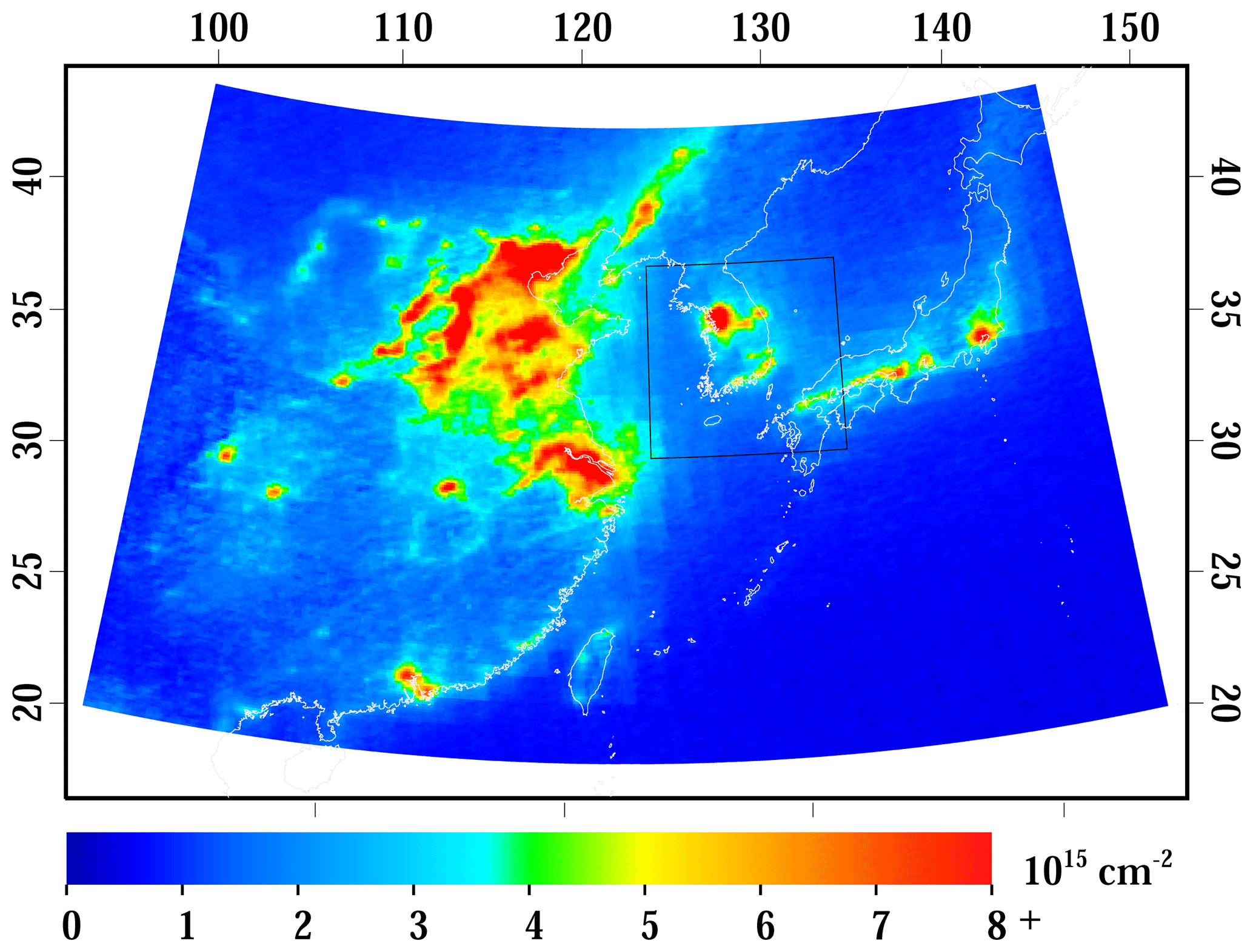
Figure 1Warm-season averaged (May–September) NO2 tropospheric vertical column content using the OMI-standard NO2 product for the years 2015–2017 in East Asia. The 4 km × 4 km WRF-Chem domain is outlined over the Korean Peninsula.

Figure 2(a) OMI-standard NO2 product averaged over a 9-month period, April–June 2015–2017, (b) the OMI-regional NO2 product with only the air mass factor adjustment averaged over the same time frame, and (c) the ratio between the two products: (b)∕(a). (d) Same as (a), (e) the OMI-regional NO2 product with the air mass factor adjustment and spatial kernel averaged over the same time frame and (f) the ratio between the two products: (e)∕(d).
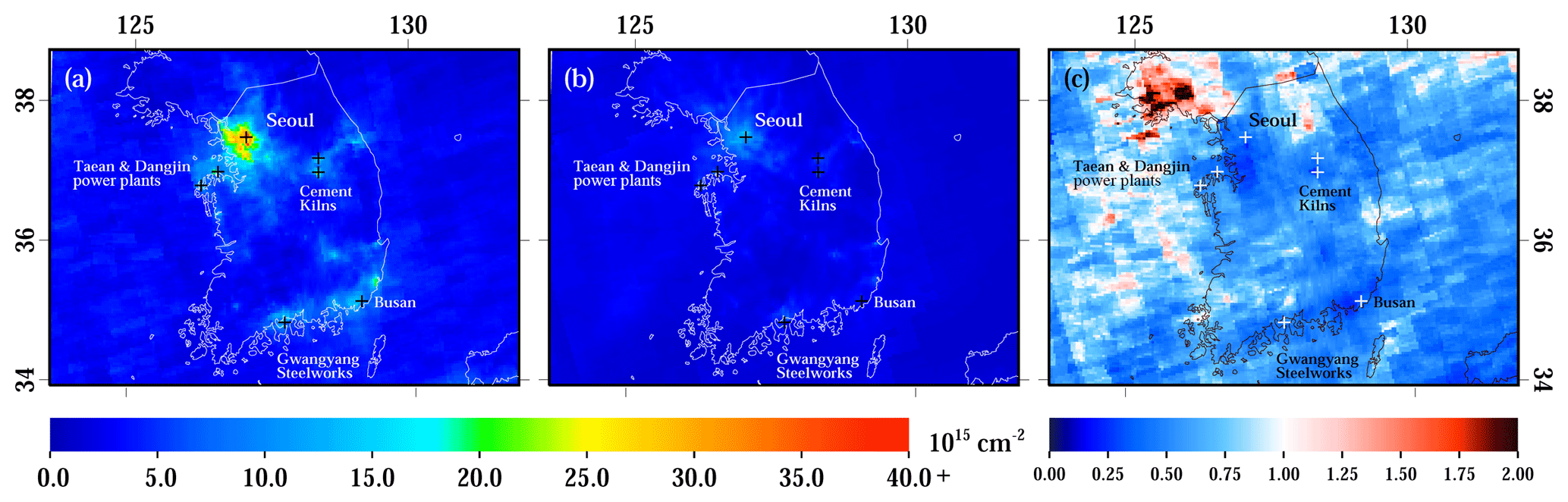
Figure 3(a) The OMI-regional NO2 product with the air mass factor adjustment and spatial kernel averaged during the month of May 2016, (b) the WRF-Chem model simulation showing only days with valid OMI measurements, and (c) the ratio between the two products. On average, there are only nine valid OMI pixels per month observed at any given location on the Korean Peninsula during May 2016.
3.2 Calculation of new OMI tropospheric column NO2
In Fig. 2, we plot the OMI-standard and OMI-regional products over South Korea. The left panels are identical and show the OMI-standard product for April–June 2015–2017. Figure 2b shows a regional product in which only the air mass factor (AMF) correction is applied. Figure 2e shows a regional product in which the air mass factor correction and spatial averaging kernel (AMF + SK) are applied. The regional product yields larger OMI NO2 values throughout the majority of the Korean Peninsula. Areas near major cities (e.g., Seoul), power plants, steel mills, and cement kilns have OMI NO2 values that are >1.25 times larger in the regional AMF product and >2 times larger in the regional AMF + SK product. There are two reasons for the larger OMI NO2 signals: the air mass factors in polluted regions are now smaller (Russell et al., 2011; Goldberg et al., 2017) and the spatial weighting kernel allocates a large portion of the OMI NO2 signal into a smaller region (Kim et al., 2016).
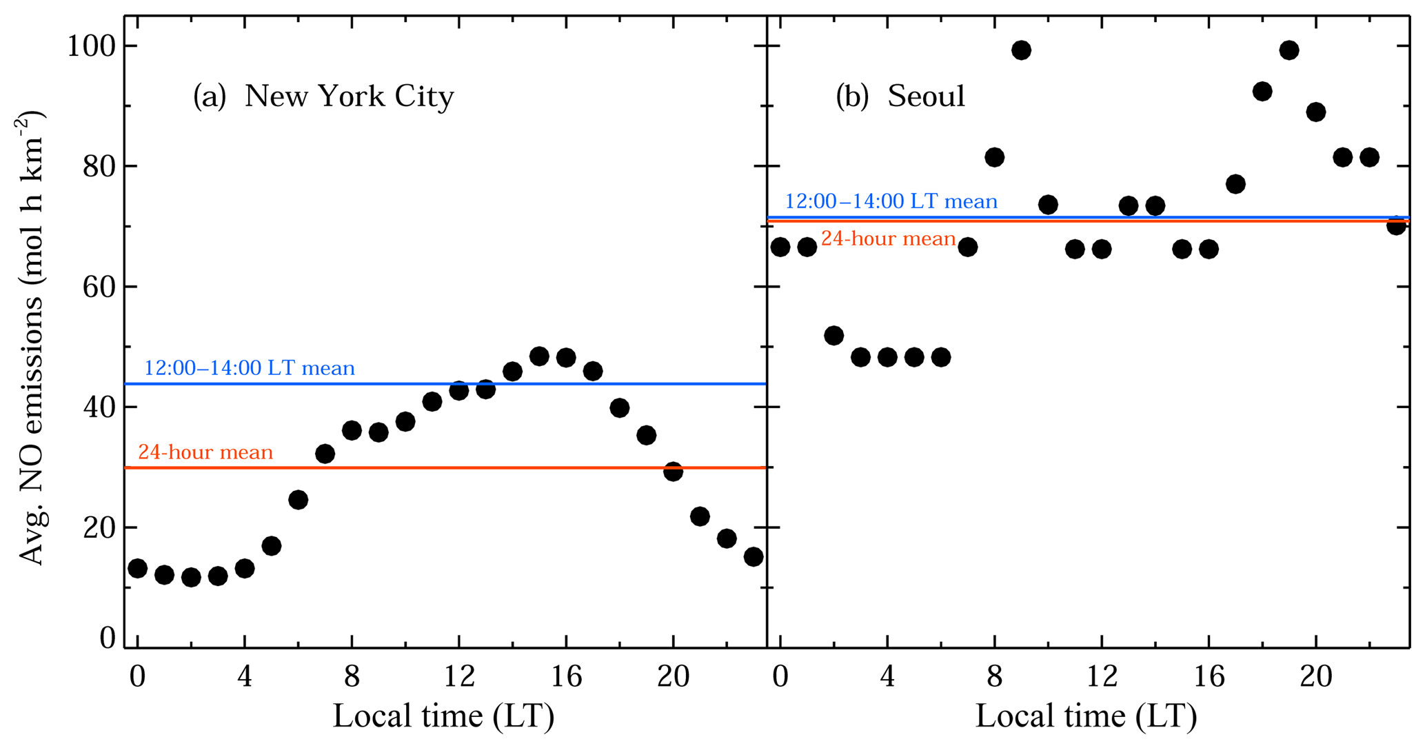
Figure 4The diurnal profile of NOx emissions rates processed from the bottom-up inventory. (a) The diurnal profile of NOx emissions rates during a weekday in New York City during July 2011 using SMOKE as the emissions preprocessor (Goldberg et al., 2016). (b) The diurnal profile of emissions rates during a weekday in Seoul during May 2016 using EPRES as the emissions preprocessor. Emissions profiles in the right panel were used in the WRF-Chem simulation.
3.3 OMI-regional vs. WRF-Chem
We now compare the OMI-regional product to tropospheric vertical columns from the WRF-Chem model simulation directly. In Fig. 3, we compare the regional satellite product (AMF + SK) to the WRF-Chem simulation over the Korean Peninsula. In most areas, the modeled tropospheric column NO2 is of smaller magnitude than inferred by the satellite. In the area within 40 km of the Seoul city center, modeled tropospheric vertical columns are 44 % smaller than observed tropospheric vertical column in the regional AMF + SK product. We posit four reasons as to why the model simulation calculates columns that are consistently smaller. First, our WRF-Chem simulation uses a reduced hydrocarbon gas-phase chemical mechanism. This fast-calculating mechanism implemented in WRF-Chem for regional climate assessments (Pfister et al., 2014) and used during KORUS-AQ for forecasting does not quickly recycle alkyl nitrates back to NO2; this will cause NO2 to be too low. While an underestimate of the chemical conversion to NO2 in WRF-Chem is a contributor to the underestimate, it likely does not account for the entire discrepancy; Canty et al. (2015) suggest that by shortening the lifetime of alkyl nitrates in the chemical mechanism, NO2 will increase by roughly 3 % in urban areas and 18 % in rural areas. Second, an underestimate in VOC emissions would have an impact on peroxyacyl and alkyl nitrate formation, and should enhance the effective NOx lifetime (Romer et al., 2016). Third, the temporal allocation of bottom-up emissions inventories can be a very significant source of uncertainty (Mues et al., 2014). The temporal allocation of the bottom-up South Korean NOx emissions is such that the early afternoon rate during the OMI overpass time (between 12:00 and 14:00 local time) is approximately equal to the 24 h averaged rate (Fig. 4). For comparison, in the eastern US, the early afternoon emissions rate is 1.35 larger than the 24 h averaged emissions rate. Thus, there are scenarios in which the temporal allocation can be up to 35 % different in the midafternoon during the OMI overpass time. We are not suggesting that the South Korean emissions inventory should have the diurnal profile of the US or vice versa, but instead that there are scenarios in which the temporal allocation can vary widely. This substantiates the future use of geostationary satellites to better constrain this temporal allocation uncertainty. Lastly, the remaining difference will likely be due to an underestimate in the emissions inventory.
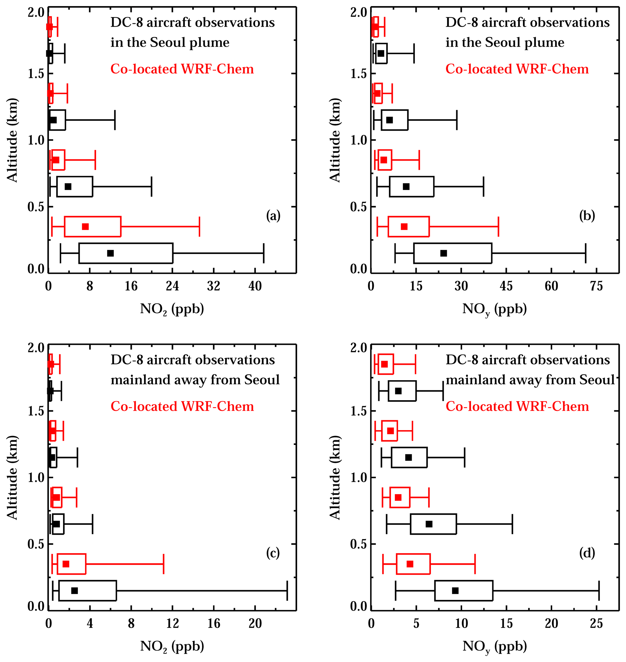
Figure 5Measurements from the DC-8 aircraft binned by altitude in black. Co-located WRF-Chem observations within the same altitude bin as the aircraft observations are plotted above in red. Square dots represent the median values. Boxes represent the 25th and 75th percentiles, while whiskers represent the 5th and 95th percentiles. (a) Comparison of NO2 in the Seoul plume (SW corner: 37.1∘ N, 127.05∘ E; NE corner: 37.75∘ N, 127.85∘ E), (b) comparison of NOy in the Seoul plume, (c) comparison of NO2 in areas outside of the Seoul metropolitan area on the Korean Peninsula (SW corner: 34.0∘ N, 126.4∘ E; NE corner: 37.1∘ N, 130.0∘ E), and (d) comparison of NOy in areas outside of the Seoul metropolitan area on the Korean Peninsula.
3.4 Comparing WRF-Chem to aircraft measurements
When comparing the model simulation to in situ observations from the UC-Berkeley NO2 instrument aboard the aircraft, we find that NO2 concentrations are substantially larger than the model when spatially and temporally collocated in the immediate Seoul metropolitan area (Fig. 5). The comparison isolates the NO2 within the lowermost boundary layer as the primary contributor to the tropospheric column underestimate. When comparing aircraft NO2 to modeled NO2 in other areas of the Korean Peninsula, the underestimate is smaller.
When comparing the model simulation of NOy to observations of the same quantity observed from the aircraft, we find a similarly large underestimate. NOy observed on the aircraft is roughly a factor of 2 larger at all altitudes below 2 km. This suggests that errors in NO2 recycling (NO2↔NOy) are not the main cause of the NO2 discrepancies seen in the satellite and aircraft comparison (also see Fig. 9). Instead, there must be errors in the NOy production (i.e., NOx emissions rates are too low) or removal rates (i.e., NOy deposition rates are too slow).
3.5 Comparison of OMI NO2 to Pandora NO2
To quantify the skill of the regional OMI NO2 product, we compare the new total NO2 vertical columns from the satellite product to the same quantities observed by the Pandora instruments. In Fig. 6, monthly averaged observations during May 2016 from the Pandora instrument are overlaid onto the monthly average of the three OMI NO2 satellite products. The two regional OMI NO2 products capture the magnitude and spatial variability of monthly averaged NO2 within the metropolitan region better.
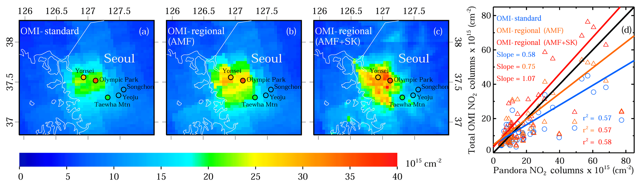
Figure 6(a) Total vertical column contents from the OMI-standard NO2 product for May 2016, (b) same quantities from the OMI-regional product with only the air mass factor adjustment (AMF) during the same time frame, (c) same quantities from the OMI-regional product with the air mass factor adjustment and spatial kernel (AMF + SK) during the same time frame, and (d) a comparison between total column contents from the three OMI NO2 products and Pandora NO2 during May 2016. An average of Pandora 2 h means co-located to valid daily OMI overpasses are overlaid in the spatial plots.
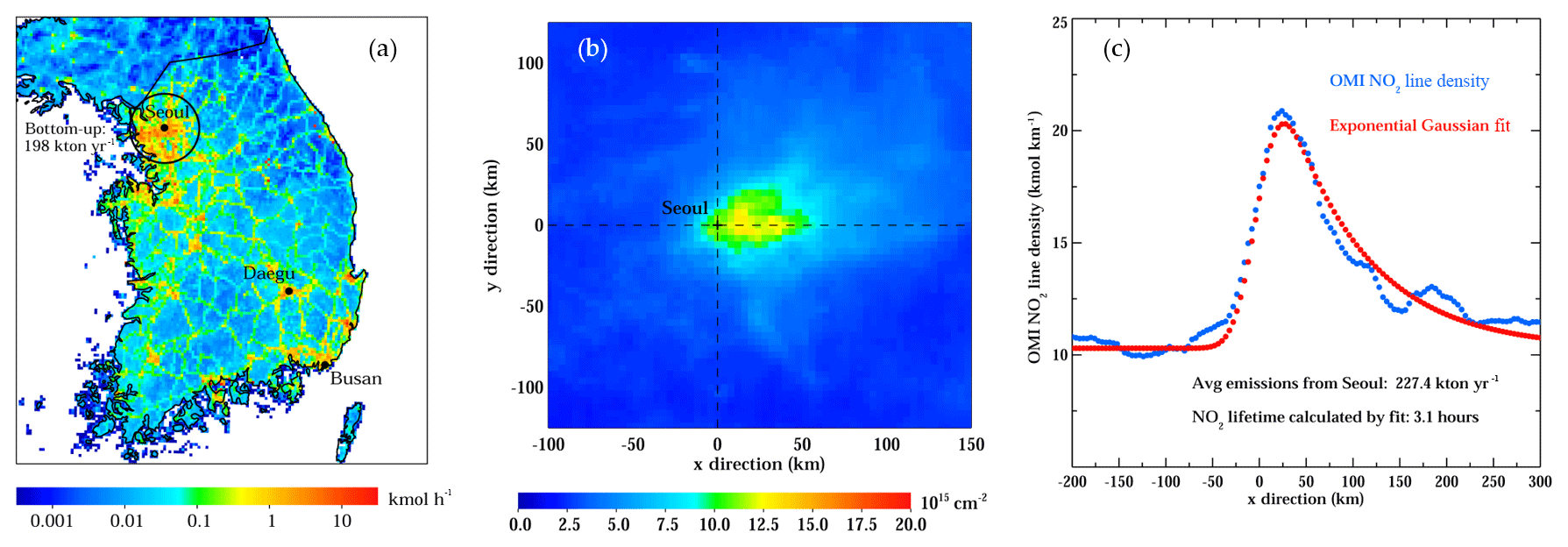
Figure 7(a) Bottom-up NOx emissions inventory compiled for the KORUS-AQ field campaign, (b) the oversampled NO2 plume rotated based on wind direction for Seoul, South Korea, from WRF-Chem (4 km × 4 km) for May 2016, and (c) NO2 line densities integrating over the 240 km across-plume width (−120 to 120 km along the y axis) and the corresponding EMG fit. NOx emissions estimates are shown in units of kt yr−1 NO2 equivalent and represent the midafternoon emissions rate.
We then compare daily Pandora observations to each daily OMI NO2 value spatially and temporally collocated with the Pandora instrument (Fig. 6). The Pandora observation is a 2 h mean centered on the midafternoon OMI overpass. The slope of the linear best fit of the standard product is 0.58, indicating that there is a consistent low bias in the satellite product when the Pandora instrument observes large values. A similar result was also found by Herman et al. (2018). The best-fit slope of the OMI-regional product with only the air mass factor adjustment (AMF) is 0.76, and the OMI-regional product with the air mass factor adjustment and spatial kernel (AMF + SK) is 1.07, indicating that the regional products capture the polluted-to-clean spatial gradients best. The correlation of daily observations to the satellite retrievals does not improve between retrievals (OMI-standard: r2=0.57, OMI-regional (AMF): r2=0.57, and OMI-regional (AMF + SK): r2=0.58). The lack of improvement in the correlation suggests that the forecasted WRF-Chem simulation is unable to capture the daily variability of NO2 plumes better than a longer-term average.
3.6 Estimating NOx emissions from Seoul
To estimate NOx emissions from the Seoul metropolitan area using a top-down satellite-based approach, we follow the exponentially modified Gaussian fitting methodology outlined in Sect. 2.5. When fit using the EMG method, the photochemical lifetime and OMI NO2 burden can be derived. Using this information, a NOx emissions rate can be inferred.
3.6.1 Validating the EMG method using WRF-Chem
The WRF-Chem simulation can serve as a test bed to assess the accuracy of the EMG method, since the bottom-up emissions used for the simulation are known. For this study, we find that for Seoul, an across-plume width of 160 km encompasses the entire NO2 downwind plume. Using the NO2 lifetime, NO2 burden, and a 160 km across-plume width, we calculate the top-down NOx emissions rate in the WRF-Chem simulation from the Seoul metropolitan area during the early afternoon (Fig. 7). We find the effective NO2 photochemical lifetime to be 3.1±1.3 h and the emissions rate to be 227±94 kt yr−1 NO2 equivalent. Uncertainties in the top-down NOx emissions are the square root of the sum of the squares of the NOx∕NO2 ratio (10 %), the OMI NO2 vertical columns (25 %), the across-plume width (10 %), and the wind fields (30 %) (Lu et al., 2015). Only the latter three terms are used to calculate the uncertainty of the NO2 lifetime (Lu et al., 2015).
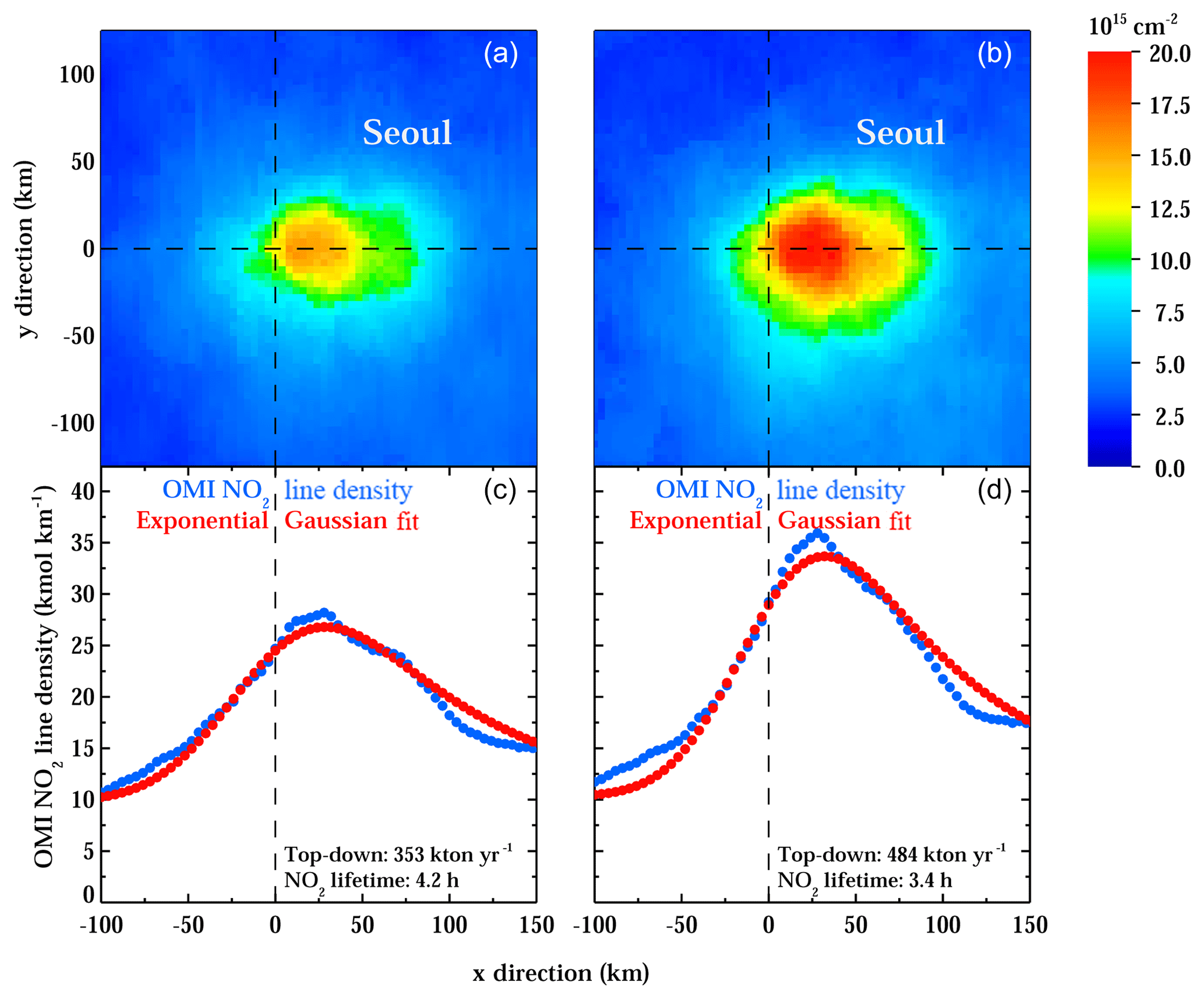
Figure 8Panels (a) and (b) represent the oversampled (4 km × 4 km) OMI NO2 plume from Seoul rotated based on wind direction over a 9-month period, April–June 2015–2017, centered on May 2016. Panels (c) and (d) represent the OMI NO2 line densities integrating over the 240 km across-plume width (−120 to 120 km along the y axis of a, b) and the corresponding EMG fit. Panels (a) and (c) are from the OMI-standard NO2 product and (b) and (d) are from the OMI-regional NO2 product. NOx emissions estimates are shown in units of kt yr−1 NO2 equivalent and represent the midafternoon emissions rate.
The NOx bottom-up emissions inventory calculated using a 40 km radius from the Seoul city center is 198 kt yr−1 NO2 equivalent. We use a 40 km radius in lieu of a larger radius because an assumption in the EMG method is that the emissions must be clustered around a single point (in this case, the city center). Therefore, the calculated emissions rate from the EMG fit is only measuring the magnitude of the perturbing emissions source, and not of smaller sources that are further from the city center. Previous studies (de Foy et al., 2014, 2015) suggest that the background level calculated by the EMG fit accounts for emissions outside the plume that are more regional and diffuse in nature. The agreement between the top-down (227 kt yr−1) and bottom-up (198 kt yr−1) approaches demonstrates the accuracy and effectiveness of the EMG method in estimating the emissions rate.
3.6.2 Deriving emissions using OMI NO2
We now calculate the top-down NOx emissions rate from the satellite data from the Seoul metropolitan area during the early afternoon (Fig. 8). Here we use the OMI standard product and the OMI NO2 retrieval without the spatial averaging kernel; only the new air mass factor is applied to this retrieval. We do not use the retrieval with the spatial averaging kernel when calculating top-down NOx emissions because the spatial averaging is strongly dependent on the wind fields in the WRF-Chem simulation, which are forecasted. Errors in the winds can greatly affect the estimate using this top-down approach (Valin et al., 2013; de Foy et al., 2014).
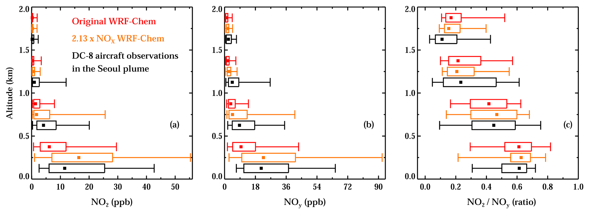
Figure 9Measurements from the DC-8 aircraft binned by altitude in black. Co-located WRF-Chem within the same altitude bin as the aircraft observations are plotted above in red for the original and in orange for the 2.13×NOx emissions simulation. Square dots represent the median values. Boxes represent the 25th and 75th percentiles, while whiskers represent the 5th and 95th percentiles. (a) Comparison of NO2 in the Seoul plume (SW corner: 37.1∘ N, 127.05∘ E; NE corner: 37.75∘ N, 127.85∘ E), (b) comparison of NOy in the Seoul plume, (c) comparison of the NO2–NOy ratio in the Seoul plume when coincident NO2 and NOy measurements are available.
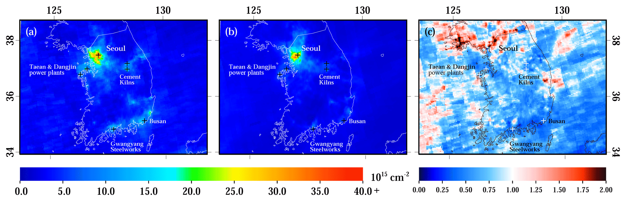
Figure 10Same as Fig. 3, but now showing the WRF-Chem simulation with NOx emissions in the Seoul metropolitan area increased by a factor of 2.13 in panel (b).
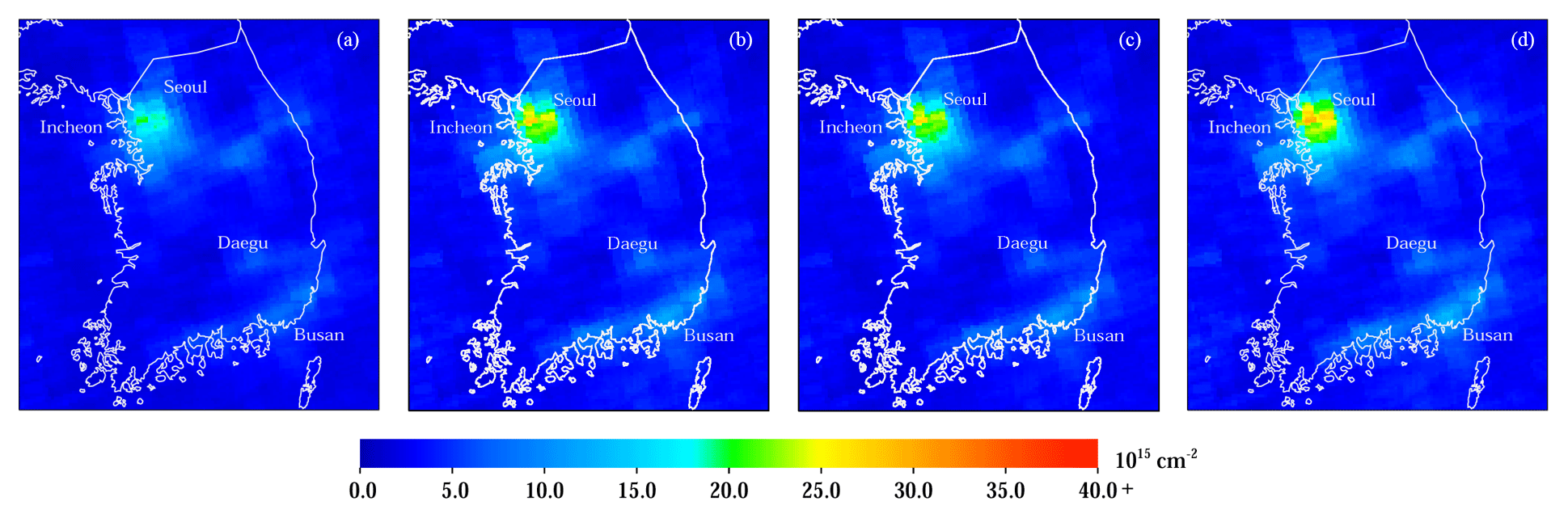
Figure 11(a) The OMI-standard product during the month of May 2016, (b) the OMI-regional NO2 product with the WRF-Chem air mass factor adjustment and spatial kernel during the same period, (c) same as (b) but using WRF-Chem NO2 profiles scaled based on the aircraft comparison, and (d) same as (b) but using the WRF-Chem simulation with NOx in the Seoul metropolitan area emissions increased by a factor of 2.13.
For the standard product, the effective NO2 photochemical lifetime is 4.2±1.7 h, while in the regional product, the effective lifetime is 3.4±1.4 h. In the standard product, we derive the NOx emissions rate to be 353±146 kt yr−1 NO2 equivalent, while in the regional product it is 484±201 kt yr−1 NO2 equivalent. Emissions estimates using satellite products with coarse-resolution air mass factors will yield top-down emissions estimates that are lower than in reality. In this case, the regional satellite product yields NOx emissions rates that are 37 % higher; we would expect similar results from other metropolitan regions. The top-down approach for the model simulation yielded a NOx emissions rate of 227 kt yr−1, while the top-down approach using the satellite data yielded a 484 kt yr−1 NOx emissions rate: a 53 % underestimate in the emissions inventory.
It should be noted that the NO2 photochemical lifetime derived here is a fundamentally different quantity than the NO2 lifetime observed by in situ measurements (de Foy et al., 2014; Lu et al., 2015) or derived by model simulations (Lamsal et al., 2010). This is because the lifetime calculation is extremely sensitive to the accuracy of the wind direction (de Foy et al., 2014) and spatial pattern of the emissions. Inaccuracies in the wind fields introduce noise that shortens the tail of the fit. As a result, NO2 photochemical lifetimes derived here are considered “effective” photochemical lifetimes and are generally shorter than the tropospheric column NO2 lifetimes derived by model simulations (Lamsal et al., 2010). NOx sources at the outer portions of urban areas will lead to an artificially longer NO2 lifetime. This partially compensates for the bias introduced by the wind direction. The heterogeneous topography and oscillating thermally driven wind flows (such as the Yellow Sea breeze) in the Seoul metropolitan area are effects that may bias the effective photochemical lifetime calculation. We partially account for this bias by only selecting days with strong winds (>3 m s−1); on days with faster winds speeds, the sea and mountain breeze effects are secondary to the synoptic flow.
3.7 Model simulation with increased NOx emissions
To test whether an increase in the NOx emissions rate is appropriate for the Seoul metropolitan area, we conduct a simulation with NOx emissions in the Seoul metropolitan area (within a 40 km radius of the city center), which increased by a factor of 2.13, and we analyze the results for May 2016. The 2.13 increase is representative of the change suggested by the top-down method (OMI-regional: 484 kt yr−1 vs. WRF-Chem original: 227 kt yr−1). This simulation was performed slightly differently than the original simulation in that it was a continuous month-long simulation and the outer domain was nudged to the reanalysis.
When comparing the new model simulation to in situ observations from the UC-Berkeley NO2 and NCAR NOy instruments aboard the DC-8 aircraft, we find that NO2 concentrations are a bit high, but NOy concentrations are in good agreement with WRF-Chem in the boundary layer when spatially and temporally collocated in the immediate Seoul metropolitan area (Fig. 9). The NO2–NOy partitioning is captured well by both model simulations, and there is no significant change in the NO2–NOy ratio when using increased NOx emissions.
When comparing the new WRF-Chem simulation to the OMI-regional product for May 2016 (Fig. 10), we now find no significant biases in the Seoul metropolitan area. In the area within 40 km of the Seoul city center, NO2 columns are now only 11 % smaller in the new model simulation. The better agreement in NO2 and NOy from a combination of aircraft and satellite data suggests that an increase in NOx emissions by a factor of 2.13 is appropriate.
Finally, we reprocess the air mass factors for May 2016 using the newest WRF-Chem simulation. In Fig. 11, we show the OMI-standard product, the OMI-regional product with no scaling of the a priori profiles from the original WRF-Chem simulation, the OMI-regional product with scaling of the original a priori profiles, and the OMI-regional product with a priori profiles from the new WRF-Chem simulation. While using the new a priori profiles increases the OMI NO2 retrieval further by 8 %, this change is much smaller than the 37 % increase associated with switching models and model resolution (i.e., standard vs. regional product).
In this work, we use a high-resolution (4 km × 4 km) WRF-Chem model simulation to recalculate satellite NO2 air mass factors over South Korea. We also apply a spatial averaging kernel to better account for the subpixel variability that cannot be observed by OMI. The regional OMI NO2 retrieval yields increased tropospheric columns in city centers and near large industrial areas. In the area within 40 km of the Seoul city center, OMI NO2 values are 1.37 larger in the regional product. Areas near large industrial sources have OMI NO2 values that are >2 times larger. The increase in remotely sensed tropospheric vertical column contents in the Seoul metropolitan area is in better agreement with the Pandora NO2 spectrometer measurements acquired during the KORUS-AQ field campaign.
Using the regional OMI NO2 product with only the air mass factor correction applied, we derive the NOx emissions rate from the Seoul metropolitan area to be 484±201 kt yr−1, while the standard NASA OMI NO2 product gives an emissions rate of 353±146 kt yr−1. The WRF-Chem simulation yields a midafternoon NOx emissions rate of 227±94 kt yr−1. This suggests an underestimate in the bottom-up NOx emissions from Seoul metropolitan area by 53 %, when compared to the 484 kt yr−1 emissions rate from our top-down method. When comparing observed OMI NO2 to the WRF-Chem model simulation, we find similar underestimates of NO2 in the Seoul metropolitan area. The effective photochemical lifetime derived in the Seoul plume is 4.2±1.7 h using the standard OMI NO2 product and 3.4±1.4 h using the regional product. The regional product yields shorter NO2 lifetimes, although it is not a statistically significant difference. Finally, we show that a WRF-Chem simulation with an increase in the NOx emissions by a factor of 2.13 yields a better comparison with aircraft observations of NO2 and NOy and is in better agreement with the OMI-regional NO2 product developed herein.
It should be noted that the Seoul metropolitan area has complex geographical features, which adds further uncertainty to this analysis. The area has large topographical changes over short distances, including many hills (>500 m) within the metropolitan area. Furthermore, the city is in close proximity to the Yellow Sea, which causes the area to be affected by sea breeze fronts, especially in the springtime, which is our period of focus. The localized mountain and sea breezes may not be fully captured by our 4 km × 4 km WRF-Chem simulation used to derive the OMI-regional product or the ERA-Interim dataset used to calculate top-down NOx emissions. The effects of these features on local air quality have been documented elsewhere in the literature (Kim and Ghim, 2002; Lee et al., 2008; Ryu et al., 2013). Nevertheless, the 4 km × 4 km simulation will capture topography and mesoscale phenomena better than a coarse global model and further supports the benefits of WRF-Chem over a global model to derive NO2 vertical column contents.
We hypothesize that the temporal allocation of NOx emissions in the bottom-up emissions inventory is a large remaining uncertainty. The satellite-derived emissions rates are instantaneous rates at the time of the OMI overpass (∼ 13:45 local time). This is a different quantity than a bottom-up NOx emissions inventory, which is often a daily averaged or monthly averaged emissions rate. For this study, we only attempt to derive a midafternoon NOx emissions rate. Subsequently, we make sure to compare this to the midafternoon NOx emissions rate from WRF-Chem. While bottom-up studies provide estimates of the diurnal variability of NOx emissions, these are very difficult to confirm from top-down approaches. Due to a consistent midafternoon overpass time, OMI or TROPOMI cannot address this issue. Due to boundary layer dynamics, this is also very difficult to constrain from ground-based and aircraft measurements. In the future, observations from a geostationary satellite instruments such as the Geostationary Environment Monitoring Spectrometer (GEMS) and Tropospheric Emissions: Monitoring Pollution (TEMPO) will be integral in constraining the ratio of the midafternoon emissions rate to the 24 h averaged emissions rate.
Our gridded OMI NO2 products and output from our WRF-Chem simulations can be obtained by contacting the corresponding author, Daniel Goldberg (dgoldberg@anl.gov). All data from the KORUS-AQ field campaign can be downloaded freely from https://doi.org/10.5067/Suborbital/KORUSAQ/DATA01 (KORUS-AQ, 2019). Operational NO2 column data from the OMI sensor is available at https://doi.org/10.5067/Aura/OMI/DATA2017 (Krotkov et al., 2018).
DLG wrote the paper, processed the satellite data, and developed all figures. PES conducted the WRF-Chem simulation and provided general advice and guidance throughout the project. LNL provided guidance on using the NASA OMI NO2 product. BdF and ZL provided guidance on using the EMG top-down method. JHW, YK, and JK prepared the monthly emissions. MG processed the monthly emissions for use in the WRF-Chem simulation. GC and DGS provided general advice and guidance throughout the project. All co-authors edited the paper for clarity.
The authors declare that they have no conflict of interest.
The US Government retains for itself, and others acting on its behalf, a paid-up nonexclusive, irrevocable worldwide license in said article to reproduce, prepare derivative works, distribute copies to the public, and perform publicly and display publicly, by or on behalf of the Government.
This publication was developed using funding from the NASA KORUS-AQ science
team and the NASA Atmospheric Composition Modeling and Analysis Program
(ACMAP). We would like to thank the NASA Pandora Project Team, including
Jay Herman and Bob Swap of the NASA Goddard Space Flight Center, Jim Szykman
of EPA, and the ESA-Pandonia team from Luftblick in supporting the deployment
and maintenance of the Pandora instruments as well as the acquisition and
processing of those observations during KORUS-AQ. We would also like to thank
Ron Cohen of UC-Berkeley and his research group for their observations of
NO2 from the DC-8 aircraft during this same time period, and Andy
Weinheimer of NCAR and his research group for their observations of
NOy from the DC-8 aircraft. We would also like to thank
Louisa Emmons and Gaby Pfister for their support in running the WRF-Chem
simulation. Additionally, we would like to thank Jim Crawford of NASA Langley
and Barry Lefer of NASA Headquarters for their input on this research
article. The submitted paper has been created by UChicago Argonne, LLC,
Operator of Argonne National Laboratory (“Argonne”). Argonne, a US
Department of Energy Office of Science laboratory, is operated under contract
no. DE-AC02-06CH11357.
Edited by: Jason
West
Reviewed by: two anonymous referees
Allen, D. J., Pickering, K. E., Pinder, R. W., Henderson, B. H., Appel, K. W., and Prados, A.: Impact of lightning-NO on eastern United States photochemistry during the summer of 2006 as determined using the CMAQ model, Atmos. Chem. Phys., 12, 1737–1758, https://doi.org/10.5194/acp-12-1737-2012, 2012.
Beirle, S., Boersma, K. F., Platt, U., Lawrence, M. G., and Wagner, T.: Megacity Emissions and Lifetimes of Nitrogen Oxides Probed from Space, Science, 333, 1737–1739, 2011.
Boersma, K. F., Jacob, D. J., Bucsela, E. J., Perring, A. E., Dirksen, R., Yantosca, R. M., Park, R. J., Wenig, M. O., Bertram, T. H., and Cohen, R. C.: Validation of OMI tropospheric NO2 observations during INTEX-B and application to constrain NOx emissions over the eastern United States and Mexico, Atmos. Environ., 42, 4480–4497, 2008.
Boersma, K. F., Eskes, H. J., Dirksen, R. J., van der A, R. J., Veefkind, J. P., Stammes, P., Huijnen, V., Kleipool, Q. L., Sneep, M., Claas, J., Leitão, J., Richter, A., Zhou, Y., and Brunner, D.: An improved tropospheric NO2 column retrieval algorithm for the Ozone Monitoring Instrument, Atmos. Meas. Tech., 4, 1905–1928, https://doi.org/10.5194/amt-4-1905-2011, 2011.
Boersma, K. F., Vinken, G. C. M., and Tournadre, J.: Ships going slow in reducing their NOx emissions: changes in 2005–2012 ship exhaust inferred from satellite measurements over Europe, Environ. Res. Lett., 10, 074007, https://doi.org/10.1088/1748-9326/10/7/074007, 2015.
Bucsela, E. J., Krotkov, N. A., Celarier, E. A., Lamsal, L. N., Swartz, W. H., Bhartia, P. K., Boersma, K. F., Veefkind, J. P., Gleason, J. F., and Pickering, K. E.: A new stratospheric and tropospheric NO2 retrieval algorithm for nadir-viewing satellite instruments: applications to OMI, Atmos. Meas. Tech., 6, 2607–2626, https://doi.org/10.5194/amt-6-2607-2013, 2013.
Burrows, J. P., Weber, M., Buchwitz, M., Rozanov, V., Ladstatter-Weißenmayer, A., Richter, A., DeBeek, R., Hoogen, R., Bramstedt, K., Eichmann, K.-U., Eisinger, M., and Perner, D.: The Global Ozone Monitoring Experiment (GOME): Mission Concept and First Scientific Results, J. Atmos. Sci., 56, 151–175, 1999.
Canty, T. P., Hembeck, L., Vinciguerra, T. P., Anderson, D. C., Goldberg, D. L., Carpenter, S. F., Allen, D. J., Loughner, C. P., Salawitch, R. J., and Dickerson, R. R.: Ozone and NOx chemistry in the eastern US: evaluation of CMAQ/CB05 with satellite (OMI) data, Atmos. Chem. Phys., 15, 10965–10982, https://doi.org/10.5194/acp-15-10965-2015, 2015.
Chen, D., Zhou, B., Beirle, S., Chen, L. M., and Wagner, T.: Tropospheric NO2 column densities deduced from zenith-sky DOAS measurements in Shanghai, China, and their application to satellite validation, Atmos. Chem. Phys., 9, 3641–3662, https://doi.org/10.5194/acp-9-3641-2009, 2009.
Chong, H., Lee, H., Koo, J.-H., Kim, J., Jeong, U., Kim, W., Kim, S.-W., Herman, J., Abuhassan, N. K., Ahn, J.-Y., Park, J.-H., Kim, S.-K., Moon, K.-J., Choi, W.-J., and Park, S. S.: Regional Characteristics of NO2 Column Densities from Pandora Observations during the MAPS-Seoul Campaign, Aerosol Air Qual. Res., 18, 2207–2219, 2018.
Curier, R. L., Kranenburg, R., Segers, A. J. S., Timmermans, R. M. A., and Schaap, M.: Synergistic use of OMI NO2 tropospheric columns and LOTOS–EUROS to evaluate the NOx emission trends across Europe, Remote Sens. Environ., 149, 58–69, 2014.
Day, D. A., Wooldridge, P. J., Dillon, M. B., Thornton, J. A., and Cohen, R. C.: A thermal dissociation laser-induced fluorescence instrument for in situ detection of NO2, peroxy nitrates, alkyl nitrates, and HNO3, J. Geophys. Res.-Atmos., 107, 4046, https://doi.org/10.1029/2001JD000779, 2002.
Dee, D. P., Uppala, S. M., Simmons, A. J., Berrisford, P., Poli, P., Kobayashi, S., Andrae, U., Balmaseda, M. A., Balsamo, G., Bauer, P., Bechtold, P., Beljaars, A. C. M., van de Berg, L., Bidlot, J., Bormann, N., Delsol, C., Dragani, R., Fuentes, M., Geer, A. J., Haimberger, L., Healy, S. B., Hersbach, H., Hólm, E. V., Isaksen, L., Kållberg, P., Köhler, M., Matricardi, M., McNally, A. P., Monge-Sanz, B. M., Morcrette, J.-J., Park, B.-K., Peubey, C., de Rosnay, P., Tavolato, C., Thépaut, J.-N., and Vitart, F.: The ERA-Interim reanalysis: configuration and performance of the data assimilation system, Q. J. Roy. Meteor. Soc., 137, 553–597, https://doi.org/10.1002/qj.828, 2011.
de Foy, B., Krotkov, N. A., Bei, N., Herndon, S. C., Huey, L. G., Martínez, A.-P., Ruiz-Suárez, L. G., Wood, E. C., Zavala, M., and Molina, L. T.: Hit from both sides: tracking industrial and volcanic plumes in Mexico City with surface measurements and OMI SO2 retrievals during the MILAGRO field campaign, Atmos. Chem. Phys., 9, 9599–9617, https://doi.org/10.5194/acp-9-9599-2009, 2009.
de Foy, B., Wilkins, J. L., Lu, Z., Streets, D. G., and Duncan, B. N.: Model evaluation of methods for estimating surface emissions and chemical lifetimes from satellite data, Atmos. Environ., 98, 66–77, 2014.
de Foy, B., Lu, Z., Streets, D. G., Lamsal, L. N., and Duncan, B. N.: Estimates of power plant NOx emissions and lifetimes from OMI NO2 satellite retrievals, Atmos. Environ., 116, 1–11, 2015.
de Foy, B., Lu, Z., and Streets, D. G.: Satellite NO2 retrievals suggest China has exceeded its NOx reduction goals from the twelfth Five-Year Plan, Sci. Rep., 6, 35912, 2016.
Dobber, M., Kleipoo, Q., Dirksen, E., Levelt, P., Jaross, G., Taylor, S., Kelly, T., Flynn, L., Leppelmeier, G., and Rozemeijer, N.: Validation of Ozone Monitoring Instrument level 1b data products, J. Geophys. Res.-Atmos., 113, D15S06, https://doi.org/10.1029/2007JD008665, 2008.
Duncan, B. N., Lamsal, L. N., Thompson, A. M., Yoshida, Y., Lu, Z., Streets, D. G., Hurwitz, M. M., and Pickering, K. E.: A space based, high resolution view of notable changes in urban NOx pollution around the world (2005–2014), J. Geophys. Res.-Atmos., 121, 976–996, 2016.
Flynn, C. M., Pickering, K. E., Crawford, J. H., Lamsal, L., Krotkov, N., Herman, J., Weinheimer, A., Chen, G., Liu, X., and Szykman, J.: Relationship between column-density and surface mixing ratio: Statistical analysis of O3 and NO2 data from the July 2011 Maryland DISCOVER-AQ mission, Atmos. Environ., 92, 429–441, 2014.
Goldberg, D. L., Vinciguerra, T. P., Anderson, D. C., Hembeck, L., Canty, T. P., Ehrman, S. H., Martins, D. K., Stauffer, R. M., Thompson, A. M., Salawitch, R. J., and Dickerson R. R.: CAMx ozone source attribution in the eastern United States using guidance from observations during DISCOVER-AQ Maryland, Geophys. Res. Lett., 43, 2249–2258, https://doi.org/10.1002/2015GL067332, 2016.
Goldberg, D. L., Lamsal, L. N., Loughner, C. P., Swartz, W. H., Lu, Z., and Streets, D. G.: A high-resolution and observationally constrained OMI NO2 satellite retrieval, Atmos. Chem. Phys., 17, 11403–11421, https://doi.org/10.5194/acp-17-11403-2017, 2017.
Grell, G., Peckham, S. E., Schmitz, R., McKeen, S. A., Frost, G., Skamarock, W. C., and Eder, B.: Fully coupled “online” chemistry within the WRF model, Atmos. Environ., 39, 6957–6975, https://doi.org/10.1016/j.atmosenv.2005.04.027, 2005.
Han, K. M., Lee, S., Chang, L. S., and Song, C. H.: A comparison study between CMAQ-simulated and OMI-retrieved NO2 columns over East Asia for evaluation of NOx emission fluxes of INTEX-B, CAPSS, and REAS inventories, Atmos. Chem. Phys., 15, 1913–1938, https://doi.org/10.5194/acp-15-1913-2015, 2015.
Herman, J., Cede, A., Spinei, E., Mount, G., Tzortziou, M., and Abuhassan, N.: NO2 column amounts from ground-based Pandora and MFDOAS spectrometers using the direct-sun DOAS technique: Intercomparisons and application to OMI validation, J. Geophys. Res., 114, D13307, https://doi.org/10.1029/2009JD011848, 2009.
Herman, J., Spinei, E., Fried, A., Kim, J., Kim, J., Kim, W., Cede, A., Abuhassan, N., and Segal-Rozenhaimer, M.: NO2 and HCHO measurements in Korea from 2012 to 2016 from Pandora spectrometer instruments compared with OMI retrievals and with aircraft measurements during the KORUS-AQ campaign, Atmos. Meas. Tech., 11, 4583–4603, https://doi.org/10.5194/amt-11-4583-2018, 2018.
Heue, K.-P., Wagner, T., Broccardo, S. P., Walter, D., Piketh, S. J., Ross, K. E., Beirle, S., and Platt, U.: Direct observation of two dimensional trace gas distributions with an airborne Imaging DOAS instrument, Atmos. Chem. Phys., 8, 6707–6717, https://doi.org/10.5194/acp-8-6707-2008, 2008.
Hilboll, A., Richter, A., and Burrows, J. P.: Long-term changes of tropospheric NO2 over megacities derived from multiple satellite instruments, Atmos. Chem. Phys., 13, 4145–4169, https://doi.org/10.5194/acp-13-4145-2013, 2013.
Hodzic, A. and Jimenez, J. L.: Modeling anthropogenically controlled secondary organic aerosols in a megacity: a simplified framework for global and climate models, Geosci. Model Dev., 4, 901–917, https://doi.org/10.5194/gmd-4-901-2011, 2011.
Hudman, R. C., Russell, A. R., Valin, L. C., and Cohen, R. C.: Interannual variability in soil nitric oxide emissions over the United States as viewed from space, Atmos. Chem. Phys., 10, 9943–9952, https://doi.org/10.5194/acp-10-9943-2010, 2010.
Huijnen, V., Eskes, H. J., Poupkou, A., Elbern, H., Boersma, K. F., Foret, G., Sofiev, M., Valdebenito, A., Flemming, J., Stein, O., Gross, A., Robertson, L., D'Isidoro, M., Kioutsioukis, I., Friese, E., Amstrup, B., Bergstrom, R., Strunk, A., Vira, J., Zyryanov, D., Maurizi, A., Melas, D., Peuch, V.-H., and Zerefos, C.: Comparison of OMI NO2 tropospheric columns with an ensemble of global and European regional air quality models, Atmos. Chem. Phys., 10, 3273–3296, https://doi.org/10.5194/acp-10-3273-2010, 2010.
Ialongo, I., Hakkarainen, J., Hyttinen, N., Jalkanen, J.-P., Johansson, L., Boersma, K. F., Krotkov, N., and Tamminen, J.: Characterization of OMI tropospheric NO2 over the Baltic Sea region, Atmos. Chem. Phys., 14, 7795–7805, https://doi.org/10.5194/acp-14-7795-2014, 2014.
Inness, A., Blechschmidt, A.-M., Bouarar, I., Chabrillat, S., Crepulja, M., Engelen, R. J., Eskes, H., Flemming, J., Gaudel, A., Hendrick, F., Huijnen, V., Jones, L., Kapsomenakis, J., Katragkou, E., Keppens, A., Langerock, B., de Mazière, M., Melas, D., Parrington, M., Peuch, V. H., Razinger, M., Richter, A., Schultz, M. G., Suttie, M., Thouret, V., Vrekoussis, M., Wagner, A., and Zerefos, C.: Data assimilation of satellite-retrieved ozone, carbon monoxide and nitrogen dioxide with ECMWF's Composition-IFS, Atmos. Chem. Phys., 15, 5275–5303, https://doi.org/10.5194/acp-15-5275-2015, 2015.
Kim, H. C., Lee, P., Judd, L., Pan, L., and Lefer, B.: OMI NO2 column densities over North American urban cities: the effect of satellite footprint resolution, Geosci. Model Dev., 9, 1111–1123, https://doi.org/10.5194/gmd-9-1111-2016, 2016.
Kim, J. Y. and Ghim, Y. S.: Effects of the density of meteorological observations on the diagnostic wind fields and performance of photochemical modeling in the great Seoul area, Atmos. Environ., 36, 201–212, 2002.
Kleipool, Q. L., Dobber, M. R., de Haan, J. F., and Levelt, P. F.: Earth surface reflectance climatology from 3 years of OMI data, J. Geophys. Res.-Atmos., 113, D18308, https://doi.org/10.1029/2008JD010290, 2008.
KORUS-AQ: Korea-United States Air Quality Field Study, https://doi.org/10.5067/Suborbital/KORUSAQ/DATA01, 2019.
Krotkov, N. A., McLinden, C. A., Li, C., Lamsal, L. N., Celarier, E. A., Marchenko, S. V., Swartz, W. H., Bucsela, E. J., Joiner, J., Duncan, B. N., Boersma, K. F., Veefkind, J. P., Levelt, P. F., Fioletov, V. E., Dickerson, R. R., He, H., Lu, Z., and Streets, D. G.: Aura OMI observations of regional SO2 and NO2 pollution changes from 2005 to 2015, Atmos. Chem. Phys., 16, 4605–4629, https://doi.org/10.5194/acp-16-4605-2016, 2016.
Krotkov, N. A., Lamsal, L. N., Celarier, E. A., Swartz, W. H., Marchenko, S. V., Bucsela, E. J., Chan, K. L., Wenig, M., and Zara, M.: The version 3 OMI NO2 standard product, Atmos. Meas. Tech., 10, 3133–3149, https://doi.org/10.5194/amt-10-3133-2017, 2017.
Krotkov, N. A., Lamsal, L. N., Marchenko, S. V., Celarier, E. A., Bucsela, E. J., Swartz, W. H., and Veefkind, P.: OMI/Aura Nitrogen Dioxide (NO2) Total and Tropospheric Column 1-orbit L2 Swath 13×24 km V003, Greenbelt, MD, USA, Goddard Earth Sciences Data and Information Services Center (GES DISC), https://doi.org/10.5067/Aura/OMI/DATA2017, 2018.
Kuhlmann, G., Lam, Y. F., Cheung, H. M., Hartl, A., Fung, J. C. H., Chan, P. W., and Wenig, M. O.: Development of a custom OMI NO2 data product for evaluating biases in a regional chemistry transport model, Atmos. Chem. Phys., 15, 5627–5644, https://doi.org/10.5194/acp-15-5627-2015, 2015.
Lamsal, L. N., Martin, R. V., van Donkelaar, A., Steinbacher, M., Celarier, E. A., Bucsela, E., Dunlea, E. J., and Pinto, J. P.: Ground-level nitrogen dioxide concentrations inferred from the satellite-borne Ozone Monitoring Instrument, J. Geophys. Res., 113, D16308, https://doi.org/10.1029/2007JD009235, 2008.
Lamsal, L. N., Martin, R. V., van Donkelaar, A., Celarier, E. A., Bucsela, E. J., Boersma, K. F., Dirksen, R., Luo, C., and Wang, Y.: Indirect validation of tropospheric nitrogen dioxide retrieved from the OMI satellite instrument: Insight into the seasonal variation of nitrogen oxides at northern midlatitudes, J. Geophys. Res., 115, D05302, https://doi.org/10.1029/2009jd013351, 2010.
Lamsal, L. N., Krotkov, N. A., Celarier, E. A., Swartz, W. H., Pickering, K. E., Bucsela, E. J., Gleason, J. F., Martin, R. V., Philip, S., Irie, H., Cede, A., Herman, J., Weinheimer, A., Szykman, J. J., and Knepp, T. N.: Evaluation of OMI operational standard NO2 column retrievals using in situ and surface-based NO2 observations, Atmos. Chem. Phys., 14, 11587–11609, https://doi.org/10.5194/acp-14-11587-2014, 2014.
Lamsal, L. N., Duncan, B. N., Yoshida, Y., Krotkov, N. A., Pickering, K. E., Streets, D. G., and Lu, Z.: US NO2 trends (2005–2013): EPA Air Quality System (AQS) data versus improved observations from the Ozone Monitoring Instrument (OMI), Atmos. Environ., 110, 130–143, 2015.
Laughner, J. L., Zare, A., and Cohen, R. C.: Effects of daily meteorology on the interpretation of space-based remote sensing of NO2, Atmos. Chem. Phys., 16, 15247–15264, https://doi.org/10.5194/acp-16-15247-2016, 2016.
Laughner, J. L., Zhu, Q., and Cohen, R. C.: Evaluation of version 3.0B of the BEHR OMI NO2 product, Atmos. Meas. Tech., 12, 129–146, https://doi.org/10.5194/amt-12-129-2019, 2019.
Lee, H. W., Choi, H.-J., Lee, S.-H., Kim, Y.-K., and Jung, W.-S.: The impact of topography and urban building parameterization on the photochemical ozone concentration of Seoul, Korea, Atmos. Environ., 42, 4232–4246, 2008.
Levelt, P. F., Van den Oord, G. H. J., Dobber, M. R., Malkki, A., Visser, H., de Vries, J., Stammes, P., Lundell, J. O. V., and Saari, H.: The Ozone Monitoring Instrument, IEEE T. Geosci. Remote Sens., 44, 1093–1101, 2006.
Liaskos, C. E., Allen, D. J., and Pickering, K. E.: Sensitivity of tropical tropospheric composition to lightning NOx production as determined by replay simulations with GEOS-5, J. Geophys. Res.-Atmos., 120, 8512–8534, https://doi.org/10.1002/2014JD022987, 2015.
Lin, J.-T., Liu, M.-Y., Xin, J.-Y., Boersma, K. F., Spurr, R., Martin, R., and Zhang, Q.: Influence of aerosols and surface reflectance on satellite NO2 retrieval: seasonal and spatial characteristics and implications for NOx emission constraints, Atmos. Chem. Phys., 15, 11217–11241, https://doi.org/10.5194/acp-15-11217-2015, 2015.
Liu, F., Beirle, S., Zhang, Q., Dörner, S., He, K., and Wagner, T.: NOx lifetimes and emissions of cities and power plants in polluted background estimated by satellite observations, Atmos. Chem. Phys., 16, 5283–5298, https://doi.org/10.5194/acp-16-5283-2016, 2016.
Liu, F., Beirle, S., Zhang, Q., van der A, R. J., Zheng, B., Tong, D., and He, K.: NOx emission trends over Chinese cities estimated from OMI observations during 2005 to 2015, Atmos. Chem. Phys., 17, 9261–9275, https://doi.org/10.5194/acp-17-9261-2017, 2017.
Lorente, A., Folkert Boersma, K., Yu, H., Dörner, S., Hilboll, A., Richter, A., Liu, M., Lamsal, L. N., Barkley, M., De Smedt, I., Van Roozendael, M., Wang, Y., Wagner, T., Beirle, S., Lin, J.-T., Krotkov, N., Stammes, P., Wang, P., Eskes, H. J., and Krol, M.: Structural uncertainty in air mass factor calculation for NO2 and HCHO satellite retrievals, Atmos. Meas. Tech., 10, 759–782, https://doi.org/10.5194/amt-10-759-2017, 2017.
Lu, Z., Streets, D. G., de Foy, B., Lamsal, L. N., Duncan, B. N., and Xing, J.: Emissions of nitrogen oxides from US urban areas: estimation from Ozone Monitoring Instrument retrievals for 2005–2014, Atmos. Chem. Phys., 15, 10367–10383, https://doi.org/10.5194/acp-15-10367-2015, 2015.
Ma, J. Z., Beirle, S., Jin, J. L., Shaiganfar, R., Yan, P., and Wagner, T.: Tropospheric NO2 vertical column densities over Beijing: results of the first three years of ground-based MAX-DOAS measurements (2008–2011) and satellite validation, Atmos. Chem. Phys., 13, 1547–1567, https://doi.org/10.5194/acp-13-1547-2013, 2013.
Martin, R. V., Chance, K., Jacob, D. J., Kurosu, T. P., Spurr, R. J. D., Bucsela, E., Gleason, J. F., Palmer, P. I., Bey, I., and Fiore, A. M.: An improved retrieval of tropospheric nitrogen dioxide from GOME, J. Geophys. Res.-Atmos., 107, 4437, https://doi.org/10.1029/2001JD001027, 2002.
Miyazaki, K., Eskes, H., Sudo, K., Boersma, K. F., Bowman, K., and Kanaya, Y.: Decadal changes in global surface NOx emissions from multi-constituent satellite data assimilation, Atmos. Chem. Phys., 17, 807–837, https://doi.org/10.5194/acp-17-807-2017, 2017.
Mues, A., Kuenen, J., Hendriks, C., Manders, A., Segers, A., Scholz, Y., Hueglin, C., Builtjes, P., and Schaap, M.: Sensitivity of air pollution simulations with LOTOS-EUROS to the temporal distribution of anthropogenic emissions, Atmos. Chem. Phys., 14, 939–955, https://doi.org/10.5194/acp-14-939-2014, 2014.
Nault, B. A., Laughner, J. L., Wooldridge, P. J., Crounse, J. D., Dibb, J., Diskin, G., Peischl, J., Podolske, J. R., Pollack, I. B., Ryerson, T. B., Scheuer, E., Wennberg, P. O., and Cohen, R. C.: Lightning NOx Emissions: Reconciling Measured and Modeled Estimates With Updated NOx Chemistry, Geophys. Res. Lett., 44, 9479–9488, https://doi.org/10.1002/2017GL074436, 2017.
Palmer, P. I., Jacob, D. J., Chance, K. V., Martin, R. V., Spurr, R. J. D., Kurosu, T., Bey, I., Yantosca, R. M., Fiore, A., and Li, Q.: Air mass factor formulation for spectroscopic measurements from satellites: Application to formaldehyde retrievals from the Global Ozone Monitoring Experiment, J. Geophys. Res., 106, 14539–14550, 2001.
Pfister, G. G., Walters, S., Lamarque, J. F., Fast, J., Barth, M. C., Wong, J., Done, J., Holland, G., and Bruyère, C. L.: Projections of future summertime ozone over the U.S, J. Geophys. Res.-Atmos., 119, 5559–5582, https://doi.org/10.1002/2013jd020932, 2014.
Pickering, K. E., Bucsela, E. D., Ring, A., Holzworth, R., and Krotkov, N.: Estimates of lightning NOx production based on OMI NO2 observations over the Gulf of Mexico, J. Geophys. Res.-Atmos., 121, 8668–8691, 2016.
Platt, U.: Differential optical absorption spectroscopy (DOAS), Air Monitoring by Spectroscopic Technique, 127, 27–84, 1994.
Pujadas, M., Núñez, L., and Lubrani, P.: Assessment of NO2 satellite observations for en-route aircraft emissions detection, Remote Sens. Environ., 115, 3298–3312, 2011.
Rasool, Q. Z., Zhang, R., Lash, B., Cohan, D. S., Cooter, E. J., Bash, J. O., and Lamsal, L. N.: Enhanced representation of soil NO emissions in the Community Multiscale Air Quality (CMAQ) model version 5.0.2, Geosci. Model Dev., 9, 3177–3197, https://doi.org/10.5194/gmd-9-3177-2016, 2016.
Ridley, B., Ott, L., Pickering, K., Emmons, L., Montzka, D., Weinheimer, A., Knapp, D., Grahek, F., Li, L., Heymsfield, G., McGill, M., Kucera, P., Mahoney, M. J., Baumgarner, D., Schultz, M., and Brasseur, G.: Florida thunderstorms: A faucet of reactive nitrogen to the upper troposphere, J. Geophys. Res.-Atmos., 109, D17305, https://doi.org/10.1029/2004JD004769, 2004.
Romer, P. S., Duffey, K. C., Wooldridge, P. J., Allen, H. M., Ayres, B. R., Brown, S. S., Brune, W. H., Crounse, J. D., de Gouw, J., Draper, D. C., Feiner, P. A., Fry, J. L., Goldstein, A. H., Koss, A., Misztal, P. K., Nguyen, T. B., Olson, K., Teng, A. P., Wennberg, P. O., Wild, R. J., Zhang, L., and Cohen, R. C.: The lifetime of nitrogen oxides in an isoprene-dominated forest, Atmos. Chem. Phys., 16, 7623–7637, https://doi.org/10.5194/acp-16-7623-2016, 2016.
Russell, A. R., Valin, L. C., Bucsela, E. J., Wenig, M. O., and Cohen, R. C.: Space-based constraints on spatial and temporal patterns of NOx emissions in California, 2005–2008, Environ. Sci. Technol., 44, 3608–3615, 2010.
Russell, A. R., Perring, A. E., Valin, L. C., Bucsela, E. J., Browne, E. C., Wooldridge, P. J., and Cohen, R. C.: A high spatial resolution retrieval of NO2 column densities from OMI: method and evaluation, Atmos. Chem. Phys., 11, 8543–8554, https://doi.org/10.5194/acp-11-8543-2011, 2011.
Ryu, Y.-H., Baik, J.-J., Kwak, K.-H., Kim, S., and Moon, N.: Impacts of urban land-surface forcing on ozone air quality in the Seoul metropolitan area, Atmos. Chem. Phys., 13, 2177–2194, https://doi.org/10.5194/acp-13-2177-2013, 2013.
Saide, P. E., Carmichael, G. R., Liu, Z., Schwartz, C. S., Lin, H. C., da Silva, A. M., and Hyer, E.: Aerosol optical depth assimilation for a size-resolved sectional model: impacts of observationally constrained, multi-wavelength and fine mode retrievals on regional scale analyses and forecasts, Atmos. Chem. Phys., 13, 10425–10444, https://doi.org/10.5194/acp-13-10425-2013, 2013.
Saide, P. E., Kim, J., Song, C. H., Choi, M., Cheng, Y., and Carmichael, G. R.: Assimilation of next generation geostationary aerosol optical depth retrievals to improve air quality simulations, Geophys. Res. Lett., 41, 2014GL062089, https://doi.org/10.1002/2014gl062089, 2014.
Skamarock, W. C., Klemp, J. B., Dudhia, J., Gill, D. O., Barker, D. M., Wang, W., and Powers, J. G.: A description of the advanced research WRF version 3, NCAR Technical Note, NCAR/TN468+STR, https://doi.org/10.5065/D68S4MVH, 2008.
Souri, A. H., Choi, Y., Jeon, W., Li, X., Pan, S., Diao, L., and Westenbarger, D. A.: Constraining NOx emissions using satellite NO2 measurements during 2013 DISCOVER-AQ Texas campaign, Atmos. Environ., 131, 371–381, 2016.
Souri, A. H., Choi, Y., Jeon, W., Woo, J., Zhang, Q., and Kurokawa, J.: Remote sensing evidence of decadal changes in major tropospheric ozone precursors over East Asia, J. Geophys. Res.-Atmos., 122, 2474–2492, https://doi.org/10.1002/2016JD025663, 2017.
Streets, D. G., Canty, T., Carmichael, G. R., de Foy, B., Dickerson, R. R., Duncan, B. N., Edwards, D. P., Haynes, J. A., Henze, D. K., Houyoux, M. R., Jacob, D. J., Krotkov, N. A., Lamsal, L. N., Liu, Y., Lu, Z., Martin, R. V., Pfister, G. G., Pinder, R. W., Salawitch, R. J., and Wecht, K. J.: Emissions estimation from satellite retrievals: A review of current capability, Atmos. Environ., 77, 1011–1042, 2013.
Thornton, J. A., Wooldridge, P. J., and Cohen R. C.: Atmospheric NO2: In situ laser-induced fluorescence detection at parts per trillion mixing ratios, Anal. Chem., 72, 528–539, 2000.
Valin, L. C., Russell, A. R., and Cohen, R. C.: Variations of OH radicals in an urban plume inferred from NO2 column measurements, Geophys. Res. Lett., 40, 1856–1860, 2013.
Vandaele, A. C., Hermans, C., Simon, P. C., Carleer, M., Colin, R., Fally, S., Merienne, M.-F., Jenouvrier, A., and Coquart, B.: Measurements of the NO2 absorption cross-section from 42 000 cm−1 to 10 000 cm−1 (238–1000 nm) at 220 K and 294 K, J. Quant. Spectrosc. Ra., 59, 171–184, 1998.
van der A, R. J., Mijling, B., Ding, J., Koukouli, M. E., Liu, F., Li, Q., Mao, H., and Theys, N.: Cleaning up the air: effectiveness of air quality policy for SO2 and NOx emissions in China, Atmos. Chem. Phys., 17, 1775–1789, https://doi.org/10.5194/acp-17-1775-2017, 2017.
van Vuuren, D. P., Bouwman, L. F., Smith, S. J., and Dentener, F.: Global projections for anthropogenic reactive nitrogen emissions to the atmosphere: an assessment of scenarios in the scientific literature, Curr. Opin. Env. Sust., 3, 359–369, 2011.
Vasilkov, A., Qin, W., Krotkov, N., Lamsal, L., Spurr, R., Haffner, D., Joiner, J., Yang, E.-S., and Marchenko, S.: Accounting for the effects of surface BRDF on satellite cloud and trace-gas retrievals: a new approach based on geometry-dependent Lambertian equivalent reflectivity applied to OMI algorithms, Atmos. Meas. Tech., 10, 333–349, https://doi.org/10.5194/amt-10-333-2017, 2017.
Vinken, G. C. M., Boersma, K. F., Maasakkers, J. D., Adon, M., and Martin, R. V.: Worldwide biogenic soil NOx emissions inferred from OMI NO2 observations, Atmos. Chem. Phys., 14, 10363–10381, https://doi.org/10.5194/acp-14-10363-2014, 2014a.
Vinken, G. C. M., Boersma, K. F., van Donkelaar, A., and Zhang, L.: Constraints on ship NOx emissions in Europe using GEOS-Chem and OMI satellite NO2 observations, Atmos. Chem. Phys., 14, 1353–1369, https://doi.org/10.5194/acp-14-1353-2014, 2014b.
Woo, J. H., Choi, K. C., Kim, H. K., Baek, B. H., Jang, M., Eum, J. H., Song, C. H., Ma, Y. I., Sunwoo, Y., Chang, L. S., and Yoo, S. H.: Development of an anthropogenic emissions processing system for Asia using SMOKE, Atmos. Environ., 58, 5–13, 2012.
Zaveri, R. A., Easter, R. C., Fast, J. D., and Peters, L. K.: Model for simulating aerosol interactions and chemistry (MOSAIC), J. Geophys. Res., 113, D13204, https://doi.org/10.1029/2007JD008782, 2008.
Zhang, L., Jacob, D. J., Boersma, K. F., Jaffe, D. A., Olson, J. R., Bowman, K. W., Worden, J. R., Thompson, A. M., Avery, M. A., Cohen, R. C., Dibb, J. E., Flock, F. M., Fuelberg, H. E., Huey, L. G., McMillan, W. W., Singh, H. B., and Weinheimer, A. J.: Transpacific transport of ozone pollution and the effect of recent Asian emission increases on air quality in North America: an integrated analysis using satellite, aircraft, ozonesonde, and surface observations, Atmos. Chem. Phys., 8, 6117–6136, https://doi.org/10.5194/acp-8-6117-2008, 2008.
Zheng, B., Tong, D., Li, M., Liu, F., Hong, C., Geng, G., Li, H., Li, X., Peng, L., Qi, J., Yan, L., Zhang, Y., Zhao, H., Zheng, Y., He, K., and Zhang, Q.: Trends in China's anthropogenic emissions since 2010 as the consequence of clean air actions, Atmos. Chem. Phys., 18, 14095–14111, https://doi.org/10.5194/acp-18-14095-2018, 2018.
Zhou, Y., Brunner, D., Boersma, K. F., Dirksen, R., and Wang, P.: An improved tropospheric NO2 retrieval for OMI observations in the vicinity of mountainous terrain, Atmos. Meas. Tech., 2, 401–416, https://doi.org/10.5194/amt-2-401-2009, 2009.
Zhou, Y., Brunner, D., Spurr, R. J. D., Boersma, K. F., Sneep, M., Popp, C., and Buchmann, B.: Accounting for surface reflectance anisotropy in satellite retrievals of tropospheric NO2, Atmos. Meas. Tech., 3, 1185–1203, https://doi.org/10.5194/amt-3-1185-2010, 2010.