the Creative Commons Attribution 4.0 License.
the Creative Commons Attribution 4.0 License.
 | 08 Feb 2019
Impact of a nitrogen emission control area (NECA) on the future air quality and nitrogen deposition to seawater in the Baltic Sea region
Johannes Bieser
Beate Geyer
Volker Matthias
Jukka-Pekka Jalkanen
Lasse Johansson
Erik Fridell
Air pollution due to shipping is a serious concern for coastal regions in Europe. Shipping emissions of nitrogen oxides (NOx) in air over the Baltic Sea are of similar magnitude (330 kt yr−1) as the combined land-based NOx emissions from Finland and Sweden in all emission sectors. Deposition of nitrogen compounds originating from shipping activities contribute to eutrophication of the Baltic Sea and coastal areas in the Baltic Sea region. For the North Sea and the Baltic Sea a nitrogen emission control area (NECA) will become effective in 2021; in accordance with the International Maritime Organization (IMO) target of reducing NOx emissions from ships. Future scenarios for 2040 were designed to study the effect of enforced and planned regulation of ship emissions and the fuel efficiency development on air quality and nitrogen deposition. The Community Multiscale Air Quality (CMAQ) model was used to simulate the current and future air quality situation. The meteorological fields, the emissions from ship traffic and the emissions from land-based sources were considered at a grid resolution of 4×4 km2 for the Baltic Sea region in nested CMAQ simulations. Model simulations for the present-day (2012) air quality show that shipping emissions are the major contributor to atmospheric nitrogen dioxide (NO2) concentrations over the Baltic Sea. In the business-as-usual (BAU) scenario, with the introduction of the NECA, NOx emissions from ship traffic in the Baltic Sea are reduced by about 80 % in 2040. An approximate linear relationship was found between ship emissions of NOx and the simulated levels of annual average NO2 over the Baltic Sea in the year 2040, when following different future shipping scenarios. The burden of fine particulate matter (PM2.5) over the Baltic Sea region is predicted to decrease by 35 %–37 % between 2012 and 2040. The reduction in PM2.5 is larger over sea, where it drops by 50 %–60 % along the main shipping routes, and is smaller over the coastal areas. The introduction of NECA is critical for reducing ship emissions of NOx to levels that are low enough to sustainably dampen ozone (O3) production in the Baltic Sea region. A second important effect of the NECA over the Baltic Sea region is the reduction in secondary formation of particulate nitrate. This lowers the ship-related PM2.5 by 72 % in 2040 compared to the present day, while it is reduced by only 48 % without implementation of the NECA. The effect of a lower fuel efficiency development on the absolute ship contribution of air pollutants is limited. Still, the annual mean ship contributions in 2040 to NO2, sulfur dioxide and PM2.5 and daily maximum O3 are significantly higher if a slower fuel efficiency development is assumed. Nitrogen deposition to the seawater of the Baltic Sea decreases on average by 40 %–44 % between 2012 and 2040 in the simulations. The effect of the NECA on nitrogen deposition is most significant in the western part of the Baltic Sea. It will be important to closely monitor compliance of individual ships with the enforced and planned emission regulations.
- Article
(11884 KB) - Companion paper
-
Supplement
(3875 KB) - BibTeX
- EndNote


Air pollution due to shipping is a serious concern for coastal regions in Europe (Viana et al., 2014; Matthias et al., 2010). Globally, nearly 70 % of the exhaust emitted from ship traffic occurs within a corridor of 400 km along the coastline (Endresen et al., 2003). Since emissions from ships can be transported in the atmosphere over several hundreds of kilometres, they have the potential to diminish the air quality in coastal areas. In addition to the primary emitted particles in the ship exhaust, secondary particles are formed in the atmosphere by oxidation of emitted gaseous precursors – nitrogen oxides (NOx) and sulfur dioxide (SO2) – during the dispersion of the ship exhaust. Mainly by contributing to the ambient levels of fine particulate matter, PM2.5 (particles with a diameter of less than 2.5 µm), emissions from ship traffic are responsible for a large number of premature deaths globally (Corbett et al., 2007). According to Sofiev et al. (2018b), the worldwide use of cleaner marine fuels with a lower content of sulfur will strongly reduce the ship-related premature mortality and morbidity by 34 % and 54 %, respectively. In northern Europe, the health-related external costs from international shipping in the Baltic Sea and North Sea are expected to decrease by 36 % between 2000 and 2020 (Brandt et al., 2013). This reduction is mainly a consequence of the introduction of the sulfur emission control area (SECA) for the Baltic Sea (enforced 2005) and North Sea (enforced 2006), which stepwise reduced sulfur content in ship fuels.
However, air emissions of NOx from ship traffic remained almost constant throughout the last decade, and the impact of NOx will remain a concern for health. Shipping emissions of NOx on the Baltic Sea are of similar magnitude as the combined land-based NOx emissions from Finland and Sweden in all emission sectors (Jalkanen and Stipa, 2009). While EU air quality legislation will lead to a decline in land-based emissions of NOx in the future, ship emissions – without more stringent emission control measures on NOx – will rise with the projected annual growth of maritime traffic in the Baltic Sea of about 5 % (Stipa et al., 2007). As a consequence, the relative importance of shipping emissions compared to land-based emission sources of NOx is expected to increase. A review of model studies on ship emissions showed that NOx emissions from international shipping on European seas could be equal to land-based emission sources in Europe (EU-27) from 2020 onwards and confirmed that the contribution of the shipping sector to future air pollution in Europe will increase (EEA, 2013).
The atmospheric transformation of emitted NOx from shipping is especially relevant for the formation of ozone (Eyring et al., 2010). Shipping emissions are estimated to play an important role in ozone (O3) levels compared to the road transport sector near the coastal zone in Europe (Tagaris et al., 2017). A regional impact study by Huszar et al. (2010) found that the contribution of shipping emissions to surface NOx levels causes an increase in surface O3 by up to 4–6 ppbv over the eastern Atlantic and western Europe. O3 can damage vegetation, reduce plant primary productivity and agricultural crop yields (Chuwah et al., 2015) and is also a serious concern for human health (EEA, 2015).
Ship exhaust emissions of NOx are further converted to gaseous nitrous acid (HNO3) through atmospheric oxidation. This conversion of nitrogen dioxide (NO2) to HNO3 takes place at a rate of approximately 5 % h−1, causing an atmospheric lifetime of NOx of about 24 h (Geels et al., 2012). HNO3 is a sticky compound, which is, in the presence of ammonia (NH3), converted by gas-phase–particle partitioning to particulate nitrate (). Nitrate is removed from the atmosphere via dry and wet scavenging, contributing to deposition of oxidized nitrogen to the sea. Atmospheric deposition of nitrogen (N)-containing compounds play a role in the eutrophication of the coastal marine environment (e.g. Paerl, 1995). Eutrophication of the sea is caused by high inputs of nutrients (nitrogen and phosphorus), resulting in the production of algal blooms, followed by the accumulation of organic material which after sedimentation results in the depletion of oxygen in the bottom water of stratified areas of the sea. Atmospheric deposition of nitrogen accounts for approximately one-third of the total nitrogen input to the Baltic Sea (HELCOM, 2011).
Several studies have used atmospheric chemistry-transport models (CTMs) to investigate the composition and fluxes of atmospheric nitrogen to the Baltic Sea basin (Hertel et al., 2003; Hongisto and Joffre, 2005; Langner et al., 2009; Hongisto, 2011; Bartnicki et al., 2011; Geels et al., 2012) mainly focusing on the influence of meteorological and climatological factors and the interannual variability of meteorological conditions. Annual atmospheric deposition of total nitrogen to the Baltic Sea basin computed with the CTM model EMEP MSC-W (Simpson et al., 2012) declined by 27 % between 1995 (305 kt yr−1) and 2015 (222 kt yr−1) (Bartnicki et al., 2017; data normalized to interannual changes in meteorological conditions). While the deposition of oxidized nitrogen decreased by 35 % during this period, reduced nitrogen, i.e. mainly NH3 and particulate ammonium (), decreased by only 12 % (Bartnicki et al., 2017). Based on atmospheric CTM calculations, it has been estimated that the atmospheric deposition of N-containing compounds originating from ship exhaust, depending on the season, can contribute to more than 50 % of the total atmospheric deposition of nitrogen in some areas of the Baltic Sea (Stipa et al., 2007).
Emissions from shipping are regulated globally by Annex VI “Regulations for the Prevention of Air Pollution from Ships” (IMO, 2008a) to the Marine Pollution Convention (MARPOL) of the International Maritime Organisation (IMO). The NOx emission reduction scheme of IMO MARPOL Annex VI is based on the tier standards as described in the NOx technical code (IMO, 2008b). Tier 1, implemented in the year 2000, introduced emission standards for ships constructed between 1 January 2000 and 1 January 2011 up to 10 % stricter than those that applied for ships built before 2000. Tier 2, implemented in 2011, enforced up to 15 % stricter standards than Tier 1 for ships constructed after 1 January 2011. Tier 1 and Tier 2 limits are worldwide and apply to all new marine diesel engines. The third regulation stage, Tier 3, will only affect ships sailing inside the designated nitrogen emission control areas (NECAs). A NECA for the Baltic Sea, North Sea and English Channel will become effective in 2021. In the following, we refer to the northern European NECA simply as the NECA. From 1 January 2021 onwards, newly built ships in the Greater North Sea and Baltic Sea have to comply with the stringent Tier 3 regulations for NOx emissions, which are approximately 75 % stricter than Tier 2. To fulfil the requirements of Tier 3, ship owners have to use abatement methods such as exhaust control technologies (catalyst converters, etc.) or use liquefied natural gas as fuel for new ships.
For the North Sea, Matthias et al. (2016), using a regional atmospheric CTM system and detailed shipping emission inventories for the present-day and future situations, estimated that, upon introduction of the NECA in 2016, levels of NO2, particulate nitrate and ozone in 2030 would not change compared to the year 2011, because the growth in ship traffic compensates for potential emission reductions. A delayed introduction of the NECA by 5 years (in 2021) would cause concentration increases of these pollutants by 10 %–15 % compared to today (Matthias et al., 2016). The study by Matthias et al. (2016) assumes an increase in ship number by 1 % yr−1, an increase in transported cargo of 2.5 % yr−1 and a ship renewal rate of 2.5 % yr−1 independently of ship size. The study considered no gains in fuel efficiency of newly built ships. Clearly, predicted consequences of the Tier 3 NOx emission regulation on future shipping emissions depend critically on the projected growth of transported volume, the increase in ship number and the share of new ships in the future fleet. In a similar study, Jonson et al. (2015) investigated the effect of the NECA introduced in 2016 on the air quality in 2030, assuming a moderate increase in ship activity. According to their future scenario, total NOx emissions in the Baltic Sea and the North Sea will be almost unchanged in 2030 compared to 2010 if the NECA is not implemented. However, implementation of the NECA in 2016 will lead to significantly lower NOx emissions from ships in 2030, resulting in slight reductions in the burden on health due to shipping (Jonson et al., 2015). The emission study by Kalli et al. (2013), which calculates the emissions separately for every ship, taking into account expected traffic growth and fleet renewal, corroborates the strong decrease in NOx shipping emissions (by 11 % in 2020 and by 79 % in 2040) when the NECA is established in 2016.
The present study is part of the BONUS project SHEBA (Sustainable Shipping and Environment of the Baltic Sea Region; http://www.sheba-project.eu, last access: 6 February 2019). The main goal of the study is to investigate the effect of the implementation of the NECA in 2021 on the air quality in the Baltic Sea region and on the total deposition of nitrogen to the Baltic Sea in 2040. In addition to the effect of the NECA regulation, we also look into possible future developments which might diminish the beneficial effect of the NECA, such as failing to achieve increased fuel efficiency of ships.
Several future shipping emission scenarios for the year 2040 were designed. These scenarios were based on the projected development of the economic growth and ship traffic volume in accordance with the study by Kalli et al. (2013). Land-based emission sources are assumed to follow the emission reduction due to current EU legislation. Three cases with respect to future air quality were considered: (1) implementation of the NECA in 2021, (2) no implementation of the NECA and (3) alternative assumptions for the fuel efficiency of the ship fleet in combination with NECA.
A regional atmospheric CTM system using the Community Multiscale Air Quality (CMAQ) model (Byun and Schere, 2006; Appel et al., 2013), similar to that used in the study by Matthias et al. (2016), was used to simulate the present-day and future air quality conditions in the Baltic Sea region. The advantage of the applied CTM system for the Baltic Sea compared to previous studies in the same region (Matthias et al., 2016; Jonson et al., 2015; Hongisto, 2014) is the higher spatial and temporal resolution of all components driving the chemistry-transport calculations. The meteorological fields, the emissions from ship traffic and the emissions from land-based sources were considered at a grid resolution of 4×4 km2 for the innermost model domain in the nested CMAQ runs. A higher resolution of shipping emissions, which are obtained based on ship positions acquired from 4 min AIS (Automatic Identification System) records and detailed ship characteristics using the Ship Traffic Emission Assessment Model (STEAM; Jalkanen et al., 2009, 2012; Johansson et al., 2013, 2017) in combination with the higher resolution of the chemistry-transport computation allow for a better resolution of the individual ship's plumes. Moreover, the high-resolution meteorology (0.025∘ grid) resolves convective precipitation, which is expected to improve the timing and amount of predicted rainfall, crucial for the determination of the nitrogen inputs to the Baltic Sea.
The focus of the present study will be on the computational model results for summer, defined as the average of the period June–August (JJA), when assessing the changes in air quality and deposition between the future scenarios and the present-day situation. In summer, emissions from shipping are highest and the photochemical conversion of the ship exhaust constituents into compounds that are readily scavenged by precipitation is faster than in other seasons. Therefore, ship-originated oxidized nitrogen deposition to the sea is highest during the summer (Hongisto, 2014). In addition, the seasonal variation of air quality indicators and of the accumulated nitrogen deposition to seawater is presented.
A first set of model runs was performed for the situation in the year 2012. The present day model results on nitrogen deposition and the air quality situation is analysed. Modelled deposition of nitrogen was evaluated in two steps: first the predicted rainfall amount and frequency are compared to daily precipitation measurements from rain gauge stations in Sweden, and second the wet deposition of oxidized and reduced nitrogen is compared against measurements of the “Cooperative Programme for Monitoring and Evaluation of the Long-range Transmission of Air Pollutants in Europe” (EMEP) programme. Present-day model results on air quality are evaluated with measurements from the regional background stations of the EMEP monitoring network in the Baltic Sea region. A companion paper by Karl et al. (2019) presents a more detailed comparison of the model results for the current air quality situation with land-based observations of air pollutant concentrations in the Baltic Sea region. The contribution of shipping emissions to the modelled concentration of air pollutants was determined from the difference between a reference run that included all emissions and a “Noship” run that excluded emissions from ship traffic (zero-out method).
A second set of model runs was performed to assess the effect of projected emissions from shipping for the year 2040. Future air quality and nitrogen deposition is analysed in order to investigate (1) the effect of establishing the NECA in 2021 compared to a future situation without NECA and (2) the effect of a lower fuel efficiency increase than expected based on a continuation of the current trend. Changes in the ship contribution to regulated air pollutants and to nitrogen deposition over seawater between the present-day simulation and the future scenario simulations are presented. Finally, recommendations with respect to the future regulations and their possible impacts and side effects are given.
2.1 CMAQ model description
Regional chemistry transport model simulations with the Community Multiscale Air Quality (CMAQ) model v5.0.1 (Byun and Ching, 1999; Byun and Schere, 2006; Appel et al., 2013, 2017) were performed to assess the effect of emissions from ship traffic on the present-day and future air qualities of the Baltic Sea region. The CMAQ model computes the air concentration and deposition fluxes of atmospheric gases and aerosols as a consequence of emission, transport and chemical transformation. The atmospheric chemistry of reactive species is treated by the Carbon Bond V mechanism (Yarwood et al., 2005), with updated toluene chemistry (Whitten et al., 2010) and chlorine radical chemistry (mechanism cb05tucl; Sarwar et al., 2012).
The aerosol scheme AERO5 is used for the formation of secondary inorganic aerosol (SIA). Aerosol growth and nucleation is simulated by three log-normal distributed modes, each represented by three moments (Binkowski and Roselle, 2003). The Aitken and accumulation modes represent PM2.5 and the coarse mode represents particulate matter with diameter >2.5 µm (PMcoarse). The instantaneous gas-phase–aerosol equilibrium partitioning of sulfuric acid (H2SO4), HNO3, hydrochloric acid (HCl) and NH3 on the fine-particle modes is solved with the ISORROPIA v1.7 mechanism (Nenes et al., 1999). Dynamic mass transfer is simulated for the coarse particle mode because large particles often do not reach equilibrium with the gas phase for typical atmospheric timescales (Meng and Seinfeld, 1996). For the coarse mode, semi-volatile inorganic species are allowed to condense and evaporate, while H2SO4 does not evaporate again from the coarse mode. Because of the dynamic mass transfer to coarse particles it is possible to use CMAQ for the simulation of chloride (Cl−) replacement by in mixed marine and urban air masses (Foley et al., 2010), which could be an important aerosol process in the Baltic Sea region.
Sea salt emissions were calculated in line by the parameterization of Gong (2003), as described in Kelly et al. (2010). Sea salt surf zone emissions were deactivated because of considerable overestimations in some coastal regions (Neumann et al., 2016b). The formation of secondary organic aerosol (SOA) from isoprene, monoterpenes, sesquiterpenes, benzene, toluene, xylene and alkanes (Carlton et al., 2010; Pye and Pouliot, 2012) is included. SOA formation pathways include the traditional two-product representation, reaction of volatile organic compounds (VOCs) to give non-volatile products, oxidative ageing of primary organic aerosol, acid-catalysed enhancement of SOA mass, oligomerization reactions and in-cloud aqueous-phase oxidation.
Three types of clouds are modelled in CMAQ: subgrid convective precipitation clouds, subgrid non-precipitating clouds and grid-resolved clouds. CMAQ simulates the aqueous-phase chemistry in all cloud types. For the two types of subgrid clouds, the cloud module in CMAQ vertically redistributes pollutants and calculates in-cloud and precipitation scavenging. Since the meteorological model provides information about the grid-resolved clouds, CMAQ subsequently does not apply further cloud dynamics for this cloud type. Subgrid clouds are only simulated in CMAQ when the meteorological driver uses a convective cloud parameterization. Hence subgrid clouds are treated by CMAQ on the coarser outer-resolution grids (16 and 64 km) but not on the 4×4 km2 model domain because the convective clouds are resolved for the fine-grid resolution by the meteorological model.
Wet deposition of gases and particles is computed by the resolved cloud model of CMAQ, which estimates how much certain vertical model layers contributed to the precipitation. The precipitation flux for each model layer is computed as a function of the non-convective precipitation rate, the sum of hydrometeors (rain, snow and graupel) and the layer thickness (see Foley et al., 2010 for details).
Dry deposition is determined as the product of the atmospheric concentration and the deposition velocity. The dry-deposition velocity is modelled in CMAQ using the resistance analogy, where resistances are defined along pathways from the atmosphere to the surface, which act in parallel or in series. Details on the deposition pathways in CMAQ can be found in Pleim and Ran (2011). The deposition velocity for particles is calculated based on the aerosol size distribution, as well as meteorological and land-use information. For large particles, the dry-deposition transfer is by turbulent air motion and by direct gravitational sedimentation. The dry-deposition algorithm for particles includes an impaction term in the coarse mode and the accumulation mode.
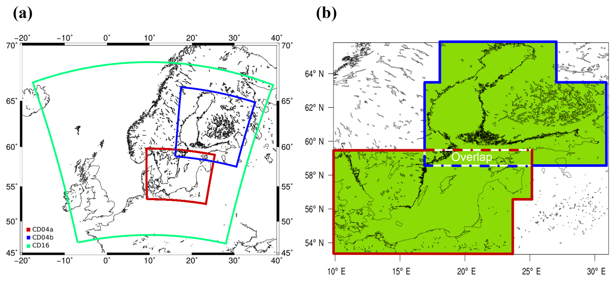
Figure 1Model nests used in the simulations with CMAQ and for the spatial maps of model results: (a) computational grid for northern Europe with 16×16 km2 resolution (CD16, green) and the high-resolution grids of 4×4 km2 for southern Baltic Sea (CD04a, dark red) and northern Baltic Sea (CD04b, dark blue). (b) Exemplary structure of spatial maps spanning from latitude 53.30∘ N (southern border) to 65.80∘ N (northern border) and longitude 9.85∘ E (western border) to 30.95∘ E (eastern border). Green shaded area is the high-resolution area which shows output from regional model runs with a grid resolution of 4×4 km2. Dark red outline marks the extent of the southern part of the Baltic Sea region and dark blue outline marks the extent of the northern part of the Baltic Sea region, for which model output from two high-resolution nests were used. For the overlap area, the arithmetic mean of results from both nests was used. In the post-processing of model results, the native Lambert conformal projection of CMAQ output was transformed to a regular lat–long grid; therefore the two outlined areas do not fill complete rectangles. The entire domain shown in panel (b) was interpolated to a uniform resolution of 0.05∘ in the post-processing. White areas of the map are covered by the output from the model nest with 16×16 km2 resolution.
In the resistance method it is assumed that the surface concentration of the chemical species is zero. However, NH3 can be both emitted from and deposited to surfaces depending on its atmospheric concentration. This bidirectional nature of the air–surface exchange can modify the atmospheric transport and environmental impact of ammonia. Bidirectional fluxes of NH3 over marine surfaces have been documented in a review by Hertel et al. (2006). In fact, inclusion of the bidirectional air–water exchange in a CTM resulted in lower overall dry deposition of NH3 to coastal waters (Sorensen et al., 2003). However, until now, the parameterization of the bidirectional flux has not been evaluated to a large extent for marine waters. Although the bidirectional flux of NH3 is implemented in CMAQ v5.0.1, the option was not used in this study. Because we are mainly interested in the differences in total nitrogen deposition due to changes in emission alone, the outcome of this study will be less affected by the sensitivity of the modelled nitrogen deposition to bidirectional fluxes of ammonia.
2.2 Set-up of the model
Nested simulations with CMAQ were performed on a horizontal resolution of 4×4 km2 to simulate the current and future air quality situation for the entire Baltic Sea region. The model was set up on a 64×64 km2 grid for the whole of Europe, subsequently on an intermediate nested 16×16 km2 grid for northern Europe, and finally on two nested 4×4 km2 grids, one for the southern Baltic Sea (Baltic major) and one for the northern Baltic Sea (including Bothnian Bay and Gulf of Finland). The nesting is visualized in Fig. 1a and the geographic details of the high-resolution domain is shown in Fig. 1b. The vertical dimension of the model extends up to 100 hPa in a sigma hybrid pressure coordinate system with 30 layers. Twenty of these layers are below approximately 2 km; the lowest layer extends to ca. 36 m above ground. A spin-up period of 1 month (December 2011) was used for the initialization of the model runs, which is sufficiently long to prevent initial conditions having an effect on the simulated atmospheric concentrations of the investigated period (year 2012).
2.3 Meteorological fields
The meteorological fields that drive the CTM were simulated with the COSMO-CLM, version 5.0, for the year 2012 (Geyer, 2014), using the ERA-Interim reanalysis and spectral nudging technique to force the model. COSMO itself is the operational weather forecast model applied and further developed by a consortium of national weather services, whereas COSMO-CLM stands for the climate mode used and developed by the limited-area modelling community (clm-community; Rockel et al., 2008).
The meteorological runs were performed first on a 0.11×0.11∘ rotated lat–long grid using 40 vertical layers up to 22 km for the whole of Europe. The output was used as the forcing of a high-resolution nested meteorology run on a 0.025×0.025∘ grid; 50 vertical levels were used for this simulation for the Baltic Sea region. The convection permitting configuration is used on the high-resolution grid, e.g. only shallow convection is based on the Tiedtke scheme, resolving convective precipitation clouds. The meteorological fields were processed afterwards using a modified version of CMAQ's Meteorology-Chemistry Interface Processor (MCIP; Otte and Pleim, 2010) to match the extension, resolution and projection of the CMAQ nested grids.
Based on the temperature anomalies and precipitation anomalies for the decade 2004–2014 for Baltic Proper, the year 2012 was chosen as the meteorological reference year for the CTM simulations. Year 2012 anomalies for 2 m temperature (±2 ∘C) and total precipitation (±25 mm) were closely aligned with the decadal average of the 2004–2014 period. The meteorological year 2012 was also used in CTM calculations of the future air quality situation to avoid complication of the interpretation of changes between the present-day and the future. Hence, future changes in the air quality are solely due to changed land-based and shipping emissions.
2.4 Boundary conditions
The initial conditions for the simulation and the lateral boundary conditions for the 64×64 km2 outer European domain (CD64) are taken from APTA global reanalysis (Sofiev et al., 2018a) and were provided by the Finnish Meteorological Institute (FMI). The global boundary conditions results have been interpolated in time and space to provide hourly boundary conditions for the outer domain. Boundary conditions for the nested intermediate grid and the two inner grids were calculated on an hourly basis from the output of the next-outer grid. For the model simulations with no shipping emissions, the full model chain was run again with all emissions except for those from ship traffic in all the CMAQ grids.
2.5 Land-based emissions
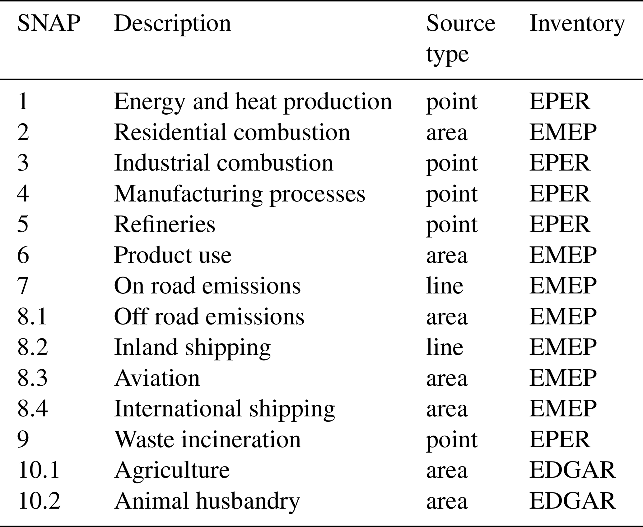
Hourly gridded emissions of NOx, sulfur oxides (), carbon monoxide (CO), NH3, PM2.5, PMcoarse and non-methane volatile organic compounds (NMVOCs) were calculated for the year 2012 using the comprehensive European emission model SMOKE-EU, which is an adaptation of the US-EPA SMOKE (Sparse Matrix Operator Kernel Emissions) model (Bieser et al., 2011a). NMVOC emissions were speciated according to the carbon bond mechanism (cb5) (Yarwood et al., 2005; Passant, 2002) of PM2.5 emissions according to the AERO5 aerosol mechanism. The SMOKE-EU emission data are based on reported annual total emissions from the European point source emission register (EPER), the official EMEP emission inventory and the EDGAR HTAP v2 database (EPER, 2018; CEIP, 2018; Olivier et al., 1999). SMOKE-EU distinguishes 10 major source sectors (including a number of subsector definitions) according to the Selected Nomenclature for sources of Air Pollution (SNAP) of the European Environmental Agency (EEA) (Table 1). For all point sources explicit plume rise calculations based on real-world stack information were performed (Bieser et al., 2011b).
The annual total emissions were temporally and spatially redistributed individually for each emission sector and grid cell. Emissions of residential heating were redistributed using the heating demand calculated from daily average temperatures (Aulinger et al., 2011). Emissions from agricultural activity and animal husbandry were disaggregated according to a fertilizer and plant growth model and meteorological parameters (Backes et al., 2016a). Finally, biogenic emissions were calculated offline with the biogenic Emission Inventory System BEIS version 3.4 (Schwede et al., 2005; Vukovich and Pierce, 2002). The SMOKE-EU emission datasets were calculated on a 5×5 km2 grid for the whole of Europe and were subsequently interpolated to the respective CMAQ model grids.
Table 1Overview of SMOKE-EU source sectors. International shipping refers to shipping outside North and Baltic seas.
3.1 Ship emission inventory for the Baltic Sea and North Sea
Shipping emissions for the Baltic Sea and North Sea with high spatial and temporal resolution for this study were obtained from STEAM (Jalkanen et al., 2009, 2012; Johansson et al., 2013, 2017). STEAM combines the AIS-based information and the detailed technical knowledge of the world fleet with principles of naval architecture. This input information is used to predict the resistance of vessels in water and the instantaneous engine power of the main and auxiliary engines on a minute-by-minute basis for each vessel that has sent AIS messages. The model predicts as output both the instantaneous fuel consumption and the emissions of selected pollutants. The dynamic modelling of shipping emissions also includes, for example, the emission control areas and regulations, emission abatement equipment on board the ships as well as fuel sulfur content modelling separately for the main and auxiliary engines (Johansson et al., 2017; Jalkanen et al., 2012).
Detailed vessel characteristics have been gathered for more than 90 000 individual ships, reported by IHS Fairplay and other ship classification societies. The AIS system provides automatic updates of the positions and instantaneous speeds of ships at intervals of a few seconds. For this study, archived and downsampled (approx. 4 min update rate) AIS messages provided by the Baltic Sea riparian states were used for 2012 and 2014, containing several hundred million AIS messages annually.
The shipping emission inventory consist of hourly updated 2×2 km2 gridded data for NOx, SOx, CO and particulate matter, which is further divided into elementary carbon (EC), organic carbon (OC), sulfate (SO4) and mineral ash. For the North Sea, ship emissions from 2011 were adopted for 2012; total ship emissions of NOx were almost unchanged between the 2 years. For Baltic Sea ship emissions are from 2012 and were provided for two vertical layers (below 36 m, from 36 to 1000 m). In CMAQ, SOx was attributed completely to SO2 and a NO:NO2 ratio of 95 : 5 was applied. Ship emissions below 36 m were attributed to the lowest vertical model layer. Ship emissions above 36 m were attributed to the second lowest layer, which appears to be justified based on findings with ship plume simulations (Chosson et al., 2008), showing that plume dispersion in the convective boundary layer (BL) is insensitive to the initial buoyancy flux.
3.2 Future scenarios for shipping emissions
Shipping in the Baltic Sea in the future is modelled in a number of scenarios taking into account the development of traffic and transport work, fleet development for different ship types (number and size), changes in fuel mixture and regulations influencing emissions and fuel consumption. Due to the long lifetime of ships it will take about 30 years after the NECA entry date until the entire ship fleet is renewed (Kalli et al., 2013) and follows the Tier 3 emission regulation for NOx. It was decided that the future regional CTM simulations for 2040 would be performed in order to see the full effect of the NECA.
3.2.1 Future baseline scenario BAU 2040
The baseline scenario for the future situation in 2040 is the so-called business-as-usual (BAU) scenario, which is constructed as a reference scenario (BAU 2040) for all other future scenarios. It accounts for current trends of economic growth and development of shipping and takes into account predefined regulations. Regarding regulations affecting emissions in air, the following are the most important ones in BAU:
-
Sulfur regulation: the Baltic and North seas are sulfur emission control areas (SECAs), where the maximum allowed sulfur (S) content in marine fuel has been gradually lowered, reaching 0.1 % S from 2015. For sea areas outside SECAs the maximum fuel sulfur content will be 0.5 % S from 2020. These regulations directly influence the emissions of SOx and have a strong impact on the particulate matter emissions.
-
NOx regulation: NOx emissions from marine engines are regulated with Tier 1 for new ships from 2000 and Tier 2 from 2011. Tier 3 is applied in NOx emission control areas and is applied for new ships in the Baltic and North seas from 2021.
-
Fuel efficiency: the regulation by IMO on Energy Efficiency Design Index (EEDI) (IMO, 2018) requires new ships to become gradually more fuel efficient. The EEDI regulation was enforced for new ships from 2015 onwards. The EEDI will influence engine emissions in a similar way to the regulations on sulfur and NOx.
The BAU scenario assumes a share of ships driven by liquefied natural gas (LNG) of about 10 % in the ship fleet in 2040. This is modelled as a fraction of new ships introduced each year that will use LNG, since retrofitting of existing ships from fuel oil to LNG is assumed to be less likely due to high costs. Since LNG is used as a means to comply with the sulfur regulations, ship types that operate mainly within SECAs are modelled as more likely to use LNG. The fuel efficiency for new ships in BAU is assumed to improve more than what is required from the EEDI regulation, following recent trends and assumption from Kalli et al. (2013), assuming that further technical improvements and more efficient operation take place. The traffic volumes are expected to continue to grow with about 1 % yr−1 on average (it varies with ship type); the current trend of using larger vessels is expected to continue as well.
3.2.2 Future scenario NoNECA 2040
The other two future scenarios, NoNECA 2040 and EEDI 2040, are deviations from the development given by the BAU scenario. In the NoNECA scenario, the nitrogen emission control area is assumed not to be implemented, i.e. all new ships up to 2040 are assumed to follow the Tier 2 NOx standard. The difference with the BAU scenario is then that new ships from 2021 follow the Tier 2 standard rather than Tier 3. The same introduction of LNG as in BAU is assumed, since the use of LNG is mainly motivated by the SECA regulation. From the difference between BAU and NoNECA, the effect of implanting the NECA on emissions can be deduced.
3.2.3 Future scenario EEDI 2040
In the EEDI scenario, improvements in fuel efficiency strictly follow the requirements of the EEDI regulation. Annual efficiency increases of 0.65 % to 1.04 %, depending on ship type, are assumed in the EEDI scenario, while the corresponding values in the BAU scenario are 1.3 % to 2.25 %. From the difference between BAU and EEDI, the effect of a lower fuel efficiency increase than expected based on the continuation of the current trend can be deduced.
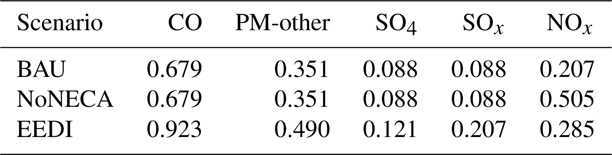
Table 2 provides emission scaling factors used in the three scenarios for future shipping emissions.
Table 2Future scenario emissions: emission scaling factors used in the three scenarios for shipping emissions for the relevant air pollutants. PM-other includes EC, OC and mineral ash. The emission scaling factors give the respective emissions in 2040 in relation to the emissions in 2012.
3.3 Future land-based emissions
The three scenarios studied here (BAU, NoNECA and EEDI) for future shipping emissions are combined with land-based emissions for 2040, which follow the currently decided emission regulations in Europe. The future land-based emission dataset for the year 2040 was created based on the present-day SMOKE-EU emission dataset (Sect. 2.5) using growth factors for each source sector and each species. The employed emission scaling factors are based on the trend between annual total emissions from the 2012 SMOKE-EU inventory and 2040 baseline emissions of the current legislation (CLE) scenario from ECLIPSE v5 (Amann et al., 2014). CLE assumes efficient enforcement of committed legislation but delays in introducing or enforcing particular laws are considered when such information was available. The scaling factors for land-based emissions, given as average of the Baltic Sea riparian states for CO, PM-other, SO4, SO2, NOx and NH3 are 0.75, 0.70, 0.45, 0.45, 0.40 and 0.80, respectively.
Ship emissions from the STEAM database were merged with the land-based emissions from the SMOKE-EU database for the Baltic Sea region and interpolated to the corresponding CMAQ domain sizes and resolutions. Total annual emissions of NOx in 2012 and in 2040 (BAU scenario) prepared for the CMAQ simulations are shown on geographic maps in Fig. 2.
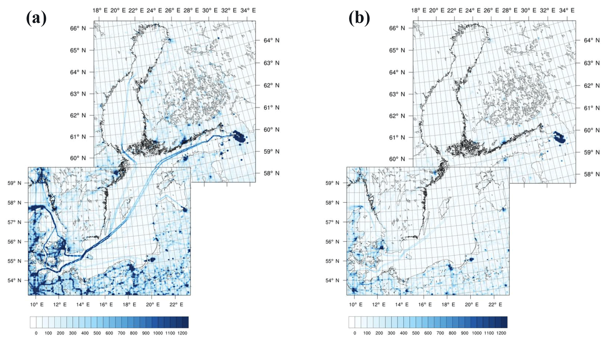
Figure 2Annual total emissions of NOx (mg(N) m−2) in the surface layer for the Baltic Sea region: (a) in 2012 and (b) in 2040 for the BAU scenario. Gridded emissions from the STEAM and SMOKE emission databases interpolated to a grid resolution of 4×4 km2 and transformed to a Lambert conformal projection for the two CMAQ high-resolution domains. Grid lines mark a lat–long grid with 0.5×0.5∘ cells.
4.1 Present-day nitrogen deposition
4.1.1 Comparison of the modelled precipitation with observations
Atmospheric deposition of nitrogen to the Baltic Sea seawater is mainly controlled by wet deposition (Hertel et al., 2003). Since wet deposition of N-containing compounds is determined as the product of the concentration of N-containing compounds dissolved in rainwater and the amount of rainfall, the accurate prediction of the amount, frequency and spatial distribution of precipitation is important. The precipitation amount and frequency from COSMO-CLM output is compared to daily precipitation measurements from rain gauge stations operated by the Swedish Meteorological and Hydrological Institute (SMHI). The rain gauge network includes 1804 precipitation stations in Sweden, which recorded daily precipitation sums during 2012. The precipitation data are available from the SMHI opendata portal (http://opendata-catalog.smhi.se/explore/, last access: 6 February 2019). Details on the methodology for comparing modelled precipitation data with these observations are given in Sect. S1 of the Supplement.
The model–observation comparison was done for the three different configurations of COSMO-CLM: 0.11∘ grid resolution with Tiedtke scheme for convection (011), 0.025∘ grid resolution with Tiedtke scheme for convection (0025_Tiedtke) and 0.025∘ grid resolution with convection-permitting configuration (0025_convper).
Finer grid resolution (0025_Tiedtke vs. 011) has a tendency to increase the rainfall over land in summer. In particular, more orographic rainfall occurs in Norway for 0025_Tiedtke compared to 011 (Fig. S1). The finer resolution improves the agreement with measured rainfall in Svealand in August, but causes too-high simulated precipitation in Norrland. The convection-permitting configuration (0025_convper) yields only small changes compared to 0025_Tiedtke. The most notable differences are the higher precipitation amounts over the Danish islands in June and more convective rainfall over southern Norway in July and August. It has been suggested that the observed inland precipitation intensity in the warm season in the southern part of Sweden is associated with convective rainfall forced by solar heating (Jeong et al., 2011). The slightly increased inland precipitation in June in 0025_convper compared to 0025_Tiedtke is in line with this suggestion.
However, COSMO-CLM predicts too-low precipitation amounts in southern Sweden in June in all three configurations. Compared to the two other configurations, 0025_convper has the highest percentage fraction of days with zero difference between model and observation both in 2012 and in summer 2012, except for northern Norrland (Fig. S2). The convection-permitting configuration performs better in particular during winter in Götaland, Svealand and southern Norrland, reducing the model–observation difference for days that are too wet. The model tends to predict too-dry weather in summer (negative bias for all three configurations) in the southern part of Sweden (Götaland and Svealand). The opposite is the case for the northern part of Sweden (Norrland), where COSMO-CLM has a positive bias (Table S2). A possible reason for the dry bias in summer could be that southern Sweden receives too little precipitation due to its location in the lee of the Norwegian mountains, where humidity is lost through excessive orographic rainfall in the simulation.
4.1.2 Comparison of the modelled wet deposition of nitrogen with observations
Wet deposition of oxidized and reduced nitrogen was evaluated with measurements of regional background stations in the Baltic Sea region for the period of 1 March to 30 November 2012. The winter months were excluded from the analysis to avoid possible artefacts associated with the collection of snow. Modelled wet deposition of nitrate, (WNO3), representing oxidized nitrogen and modelled wet deposition of ammonium, (WNH4), representing reduced nitrogen, were compared to data from the EMEP monitoring programme (Tørseth et al., 2012; EMEP, 2014) at the stations displayed on the map in Fig. 3a. Observation data were obtained from the EBAS database (http://ebas.nilu.no/, last access: 6 February 2019). Details on the methodology for comparing modelled wet deposition of nitrogen with these observations are given in Sect. S2. The comparison of the daily sum of wet deposition was done in terms of mean values (μMod and μObs), the Spearman's correlation coefficient (RSpr) and the normalized mean bias (NMB). Only days with predicted and observed rain events in common were included in the comparison. Several stations in the Baltic Sea region had only few measurements during the period. Stations with less than seven model–observation pairs were excluded from the statistical analysis. CMAQ model data from the intermediate grid (CD16) and from the high-resolution grid (CD04) are evaluated separately.
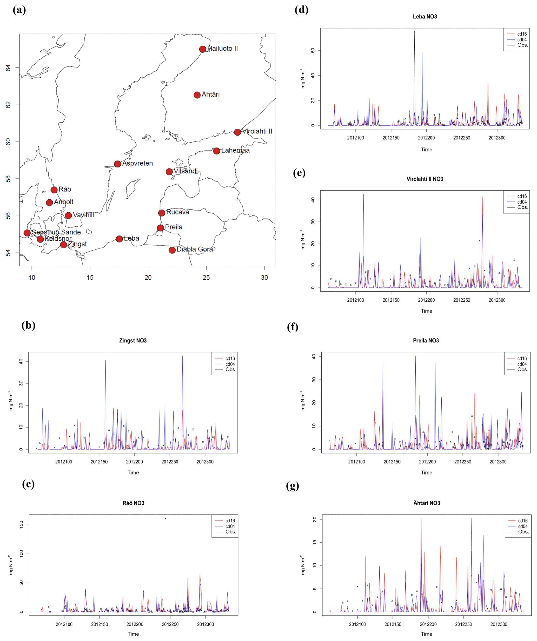
Figure 3Comparison of modelled wet deposition of nitrate (WNO3) as daily sums (in ) from the 16 km resolution grid (red) and 4 km resolution grid (blue) to observed daily sums (black crosses) at regional background stations around the Baltic Sea from the EMEP monitoring network: (a) map with stations as red circles, (b) Zingst, DE0009R, (c) Råö, SE0014R, (d) Leba, PL0004R, (e) Virolahti II, FI0017R, (f) Preila, LT0015R and (g) Ähtäri, FI0004R. Comparison time period: 1 March to 30 November 2012. All available data from simulations and observations are shown.
Plots in Fig. 3b–g show the time series modelled and observed daily sums of WNO3 at selected stations (all other stations are shown in Fig. S4). The 4 km resolution output gave higher WNO3 than the coarser CD16 output in the southern part of the Baltic Sea region (e.g. stations Zingst, Preila and Keldsnor). For the more northern stations, simulated time series of WNO3 from the two model grids are similar. The correlation between modelled and observed data improves for several stations when going from CD16 to CD04, supporting the use of a finer resolution for chemistry and transport computations in combination with high-resolution precipitation modelling. WNO3 is underestimated at all stations included in the statistical analysis (Table S3), most severely at the Finnish stations and at Zingst.
WNH4 is underestimated at all stations included in the statistical analysis (Table S4; corresponding time series are plotted in Fig. S5). The underestimation is highest for Zingst and the Finnish stations, as for WNO3. The joint underestimation of WNO3 and WNH4, especially in the northern part of the Baltic Sea region, could indicate a missing formation of particulate ammonium nitrate or too-slow conversion of NOx to HNO3 in the model. The long-range transport of particulate ammonium to the remote parts of the Baltic Sea region is further limited by the availability of particulate nitrate and sulfate (Ferm and Hellsten, 2012).
To account for the fact that the days with predicted rain often do not correspond to days with observed rain, seasonal averages (spring, summer and autumn) were calculated for WNO3 (Table S5) and WNH4 (Table S6) independently of CD04 model data and observation data. The joint underestimation of WNO3 and WNH4 at Zingst and the Finnish stations is confirmed in this analysis.
The agricultural sector, including animal husbandry, is an important source of reduced nitrogen emissions to the atmosphere (e.g. Bouwman et al., 1997). NH3 emissions from animal housing and application of manure on fields are highly relevant and can influence the formation of ammonium nitrate particles (Backes et al., 2016b). Formation of ammonium sulfate is much less sensitive to agricultural NH3 emissions because ambient background concentrations of NH3 in the model simulations are high enough to saturate the reaction-forming sulfate particles (Backes et al., 2016b). Emissions of gaseous NH3 from agriculture in northern Germany that are too low might also explain the missing WNH4 at Zingst. Annual emission totals of NH3 reported by Germany under the Long-range Transboundary Air Pollution (LRTAP) convention over the period 2009–2015 raised by ca. 9 % over prior estimates are mainly due to additional emissions from the use of inorganic and organic fertilizers (EEA, 2018, 2014). These additional reported emissions had not been included in the SMOKE-EU emission inventory at the time of the model simulations.
Measurements of gaseous NH3 from spring to autumn 2012 were available for the stations Anholt, Tange and Risoe in Denmark and for Diabla Gora in Poland. At all four stations, CMAQ overestimated the observed NH3 concentrations (NMB range 0.40–0.92), indicating that the availability of acidic compounds (such as HNO3 and H2SO4) rather than that of NH3 limited the formation of particulate ammonium in the southern part of the Baltic Sea region in the simulations.
4.1.3 Nitrogen deposition to the Baltic Sea region
Deposition of nitrogen includes particulate ammonium and nitrate as well as gaseous NO, NO2, NH3, nitrate radical (NO3), HNO3, dinitrogen pentoxide (N2O5), peroxy nitric acid (HNO4) and peroxy acetyl nitrate (PAN). Figure 4a shows the spatial distribution of the annual total (wet and dry) nitrogen deposition in 2012 from the CMAQ simulation. A strong gradient from southwest to northeast is found for the annual total nitrogen deposition, both over land and over sea. The highest nitrogen deposition (range 500–650 mg(N) m−2) to seawater is found for Belt–Kattegat and Arkona Basin areas. Seasonally accumulated nitrogen deposition to the Baltic Sea seawater shows low values (below 90 mg(N) m−2) in winter and spring and higher values (70–270 mg(N) m−2) in summer and autumn (Fig. S7). From spring to autumn there is a clear gradient between land and sea, with 2–3 times higher nitrogen deposition over land, which relates to the canopy uptake by vegetation. In winter months, the picture changes and land and sea receive similar amounts of nitrogen deposition. Over the Baltic Sea, the highest nitrogen deposition is predicted for the autumn months (SON), with maximum values of 230 mg(N) m−2 in the northern Baltic Proper.

Figure 4Present-day (2012) accumulated total deposition of nitrogen (in mg(N) m−2) in the Baltic Sea region from CMAQ model results: (a) annual deposition and (b) annual ship-related deposition. Ship contribution is only shown for the high-resolution area.
In coastal regions, nitrogen deposition is markedly higher compared to further inland. Sea salt particles can considerably increase nitrogen deposition in coastal regions, although this effect is relatively small in the Baltic Sea region and only pronounced along the coast of Denmark (Neumann et al., 2016a). Reaction of HNO3 with coarse-mode sea salt particles, when marine aerosol mixes with the polluted air from the continent, leads to a shift in fine-mode nitrate to the coarse mode through the formation of sodium nitrate (Brimblecombe and Clegg, 1988; Zhuang et al., 1999), which is essentially non-volatile in atmospheric conditions. Since coarse-mode particles are prone to deposition through gravitational settling, the nitrate formation reaction on sea salt particles may lead to enhanced deposition of nitrogen in the coastal zone (Spokes et al., 2000; Neumann et al., 2016a).
The injection of reactive nitrogen through shipping activities contributes to increased input of nitrogen to the Baltic Sea. The annual nitrogen deposition related to ship emissions (ship-related deposition) is on average 52 mg(N) m−2 over the Baltic Sea (Fig. 4b). The absolute contribution of shipping emissions (seasonal cycle shown in Fig. S8) is highest during summer, amounting to 20 mg(N) m−2 (JJA) in the Baltic Sea on average.
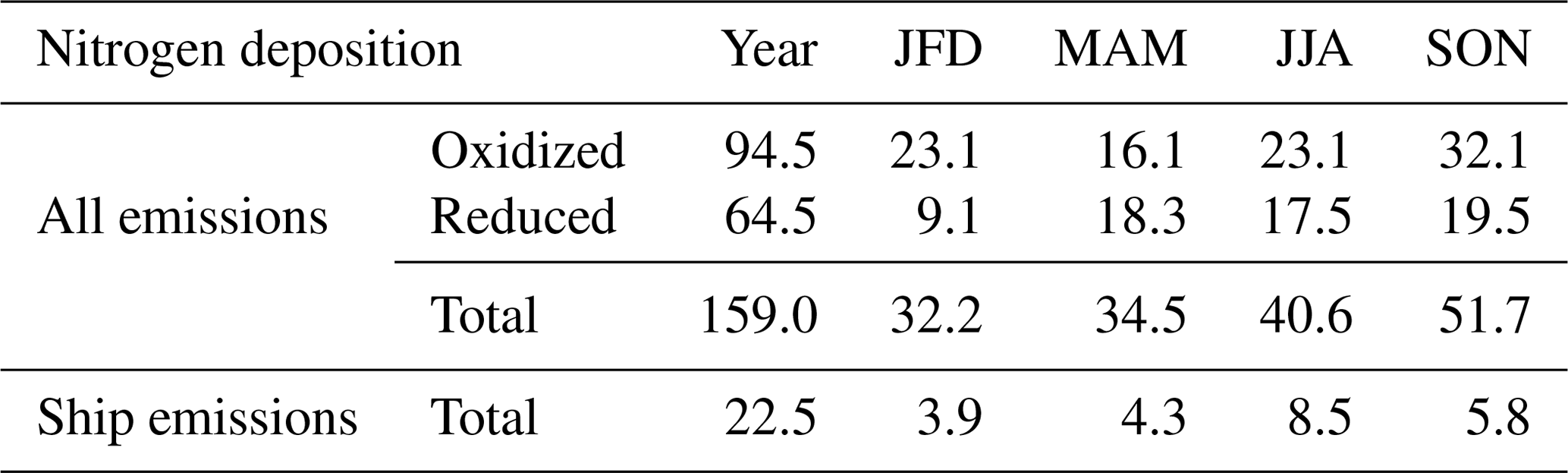
Table 3 summarizes the annual and seasonal sums of reduced, oxidized and total nitrogen deposition amounts in the seawater of the Baltic Sea together with the deposition amounts related to shipping. Total annual nitrogen deposition to Baltic Sea is 29 % lower than the estimate from the EMEP MSC-W model, normalized by the interannual changes in meteorological conditions, used in the HELCOM (Baltic Marine Environment Protection Commission – Helsinki Commission) evaluation of the Baltic Sea marine environmental status (2012: 223.6 kt N yr−1; Bartnicki et al., 2017). The annual reduced and oxidized nitrogen deposition are lower by 33 % and 27 %, respectively, than the EMEP data for 2012.
Table 3Present-day annual and seasonal nitrogen deposition amounts (kt N) in the seawater of the Baltic Sea for 2012 and ship-related nitrogen deposition from the CD04 grid. Amounts refer to a Baltic Sea surface area of 431 390 km2 including the western part of Skagerrak.
4.2 Present-day air quality
CMAQ model results for surface air concentrations of O3, NO2, SO2 and PM2.5 from the 4 km resolution grid were evaluated against measurements at regional background stations of the EMEP monitoring programme available from the EBAS database. The evaluation was done for the entire year 2012 and separately for summer (JJA) 2012. Details on the methodology for comparing modelled air pollutant concentrations with observations are given in Sect. S3.
4.2.1 Seasonality of ozone and comparison with measurements
Ozone is generated in the troposphere involving two classes of precursor compounds, VOC and NOx, in photochemical reaction cycles, initiated by the reaction of the OH radical with organic molecules. The precursors of O3 have anthropogenic and natural (or biogenic) sources, both of which are considered in the CTM simulation. On the continental scale, the formation of O3 is sustained by the oxidation of methane (CH4) and CO. In the present-day CMAQ simulation, the highest seasonal averages of the daily maximum O3 concentration were found in spring (MAM), with levels up to 50 ppbv in the southern part of the Baltic Sea region (Fig. S9), which are a consequence of the inflow of ozone-rich background air masses from the Atlantic. Photochemical production in summer leads to elevated ozone concentrations over the southern Baltic Sea (range 36–44 ppbv). In autumn and winter daily maximum O3 concentrations in the Baltic Sea region are below 34 ppbv. Modelled daily means of O3 are in good agreement with measurements at all stations (Table S7) when the entire year is considered. In summer, ozone is slightly underestimated at the stations in the southern part of the Baltic Sea region.
4.2.2 Seasonality of nitrogen dioxide and comparison with measurements
The main sources of nitrogen oxides are traffic and combustion processes. Emissions of NOx and the derived oxidation products strongly influence concentrations of ozone and particulate matter (Seinfeld and Pandis, 2005), the latter directly through the formation of nitrate aerosols and indirectly by influencing the oxidation of secondary aerosol precursors.
In spring and summer, average NO2 concentrations in proximity to the main shipping routes exceed the concentrations several times in the regional background (Fig. S10). In autumn and winter the spatial distribution of modelled seasonal averages show a gradient from south to north. High values are predicted in northern Germany, Poland and over the Danish Straits (range: 3.5–7.5 ppbv) with hotspots in the large cities (>9 ppbv). The wider spread of elevated NO2 concentrations in winter compared to summer is in accordance with a longer lifetime of NOx in winter (up to one day) compared to summer (a few hours) (Schaub et al., 2007). The evaluation of modelled NO2 based on daily concentrations for the entire year and for summer (Table S8) indicates a better performance of CMAQ over the entire year than over summer alone.
In contrast to a previous study with the CMAQ model in the North Sea region by Aulinger et al. (2016) and other multi-model air quality studies in Europe (e.g. Giordano et al., 2015), the simulations for the Baltic Sea region did not show substantial underestimation of observed NO2 daily means. The improved performance for NO2 compared to the previous study by Aulinger et al. (2016) is partly attributed to the high spatial resolution, as NOx emissions are injected into a smaller grid box volume and consequently less diluted initially.
4.2.3 Seasonality of sulfur dioxide and comparison with measurements
The main atmospheric sources of SO2 are fossil fuel combustion and metal-producing industries. The atmospheric lifetime of SO2 based on the reaction with the OH radical is about 1 week (Seinfeld and Pandis, 2005). SO2 is removed efficiently by dry deposition; the lifetime towards dry deposition is typically about 1 day. Overall, the average lifetime of SO2 in the troposphere is a few days. SO2 is converted to sulfate aerosols either via gas-phase oxidation to H2SO4 and subsequent nucleation or condensation or by uptake into cloud droplets followed by aqueous-phase oxidation. SO2 is a major air pollutant and linked to air quality and human health issues.
SO2 shows higher concentrations in autumn and winter than in spring and summer (Fig. S11). The main reason is the stable boundary layer connected with stagnant air and frequent inversions during the colder season, which causes emissions of SO2 to accumulate in the surface layer. Residential heating emissions and power plant emissions for district heating strongly contribute to the higher SO2 concentrations in winter compared to summer. Highest SO2 concentrations in autumn and winter are simulated over Poland, where levels in the cities exceed 3 ppbv. In spring and summer elevated SO2 levels over the Baltic Sea (0.9–1.8 ppbv), confined to the main shipping routes, are a sign of the influence from shipping activities. Another factor leading to lower concentrations in summer is the faster oxidation of SO2 by OH compared to other seasons.
Observed SO2 concentrations are generally overestimated (Table S9), indicating that the oxidation of SO2 in the background air is not efficient enough in the simulation. The overestimation of both SO2 and NO2 by the model corroborates the hypothesis of too-slow conversion of the primary gaseous precursors given in Sect. 4.1.2 to explain the underestimated nitrogen deposition, but it is also possible that the anthropogenic emissions of these pollutants are too high in the model.
4.2.4 Seasonality of PM2.5 and comparison with measurements
Particulate matter (PM) is a widespread air pollutant, consisting of a mixture of solid and liquid particles suspended in the air. Ambient PM2.5 comprises primary emitted and secondary PM that formed in the atmosphere. Primary PM includes OC and EC particles from anthropogenic sources such as traffic and industrial activities, as well as wind-blown soil dust and sea salt particles from natural sources. Secondary PM includes secondary inorganic and organic particles from the homogeneous and heterogeneous chemical transformation of primary gaseous precursors such as NOx, SO2, NH3 and NMVOC in the atmosphere. PM between 0.1 and 1 µm in diameter can remain in the atmosphere for days or weeks and thus be subject to long-range transport. PM2.5 is known to have adverse health effects: short-term exposure to PM2.5 is associated with respiratory and cardiovascular diseases (e.g. Pope and Dockery, 2006), while long-term exposure to PM2.5 is associated with an increase in the long-term risk of cardiopulmonary mortality (Beelen et al., 2008).
Modelled PM2.5 is highest in winter, exceeding 6 µg m−3 in most parts of the Baltic Sea region, which is attributable to the stagnant conditions and higher emissions of primary PM than in the other seasons (Fig. S12). Low temperatures in winter are favourable for the condensation of gaseous precursors to particles. In spring and autumn, PM2.5 is higher in the southern part, both over land and sea, than in the northern part of the Baltic Sea region. The high PM2.5 levels over land in the south are presumably due to a combination of land-based PM emissions, long-range-transported PM and the condensation of secondary PM from the transformation of gaseous precursor emissions. In summer, PM2.5 in the region is much smaller and shipping activities influence PM2.5 levels over the Baltic Sea, as indicated by elevated concentrations along the shipping routes in the Danish Straits and the Gulf of Finland.
For the entire year CMAQ performs quite well in the prediction of daily mean PM2.5, but in the summer period, PM2.5 is underestimated (Table S10). This is partly due to the underestimation of secondary organic aerosols by the CMAQ model. Although the capability of CMAQ to predict SOA has been improved compared to earlier versions of the model, the predicted SOA compounds make up only a small fraction of the predicted PM2.5. On the other hand, the contribution of SOA is relatively small at coastal sites (about 0.1 µg m−3) compared to inland sites (about 0.5 µg m−3) in northern Europe (Andersson-Sköld and Simpson, 2001; Gelencsér et al., 2007). Other causes for the low PM2.5 concentrations in summer could be too little formation of SIA due to the inefficient conversion of primary gaseous precursors, as stated in Sect. 4.2.3. In addition, emissions of wind-blown soil dust particles were not activated in the CMAQ simulations. A deeper investigation of the reasons for the underestimation in summer would require a detailed comparison of the individual aerosol components, which is out of the scope of the present study.
4.2.5 Summer mean ship contribution of air pollutants
The influence of shipping emissions on the present-day air quality was evaluated for the summer months. The results for the impact of shipping emissions were calculated as difference between the reference run and the run with no ship emissions (in the North and Baltic seas) in 2012. Results for the absolute and relative ship contributions in summer (as JJA average) are shown in Fig. 5 for the daily maximum O3, NO2, SO2 as well as PM2.5, and discussed in the following.
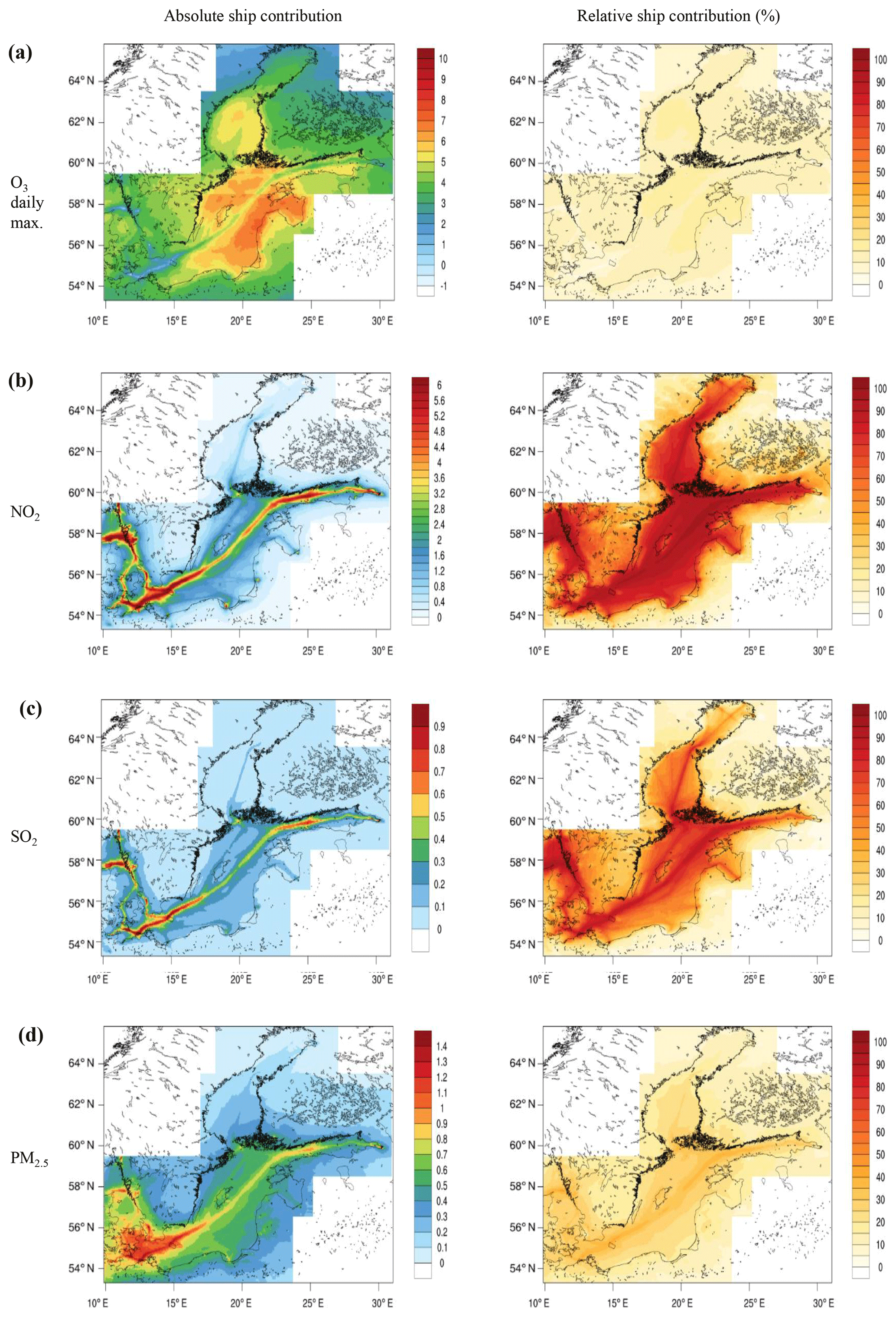
Figure 5Present-day (2012) ship contribution in the Baltic Sea region in summer (JJA) from CMAQ model results: ship-related concentration (left) for gaseous pollutants (in ppbv) and for PM2.5 (in µg m−3), percentage ship contribution (right) for (a) daily maximum O3, (b) NO2, (c) SO2 and (d) PM2.5. Ship-related contribution only shown for the high-resolution area. See text for details.
In the proximity of the main shipping routes, ozone concentrations are reduced by 10 %–20 % on spatial average in summer compared to a situation with no shipping emissions. This reduction is due to local-scale titration of O3 by NO emitted in the ship plumes. With increased distance (>100 km) from the main ship routes, photochemical ozone production takes place when NOx and CO from a ship exhaust mix with the continental emissions of NMVOC. Shipping emissions contribute to summer daily maximum O3 in the coastal areas of the Baltic states, southern Finland and eastern Sweden by up to 4.5 ppbv (ca. 20 %) (Fig. 5a). A limitation of the model results for regional surface concentrations of O3 over the Baltic Sea region is the lack of emission data on NMVOC from shipping in the STEAM inventory. Additional NMVOC emissions from shipping would enhance photochemical ozone production.
Summer mean surface air concentrations of NO2 over the Baltic Sea in the background areas without shipping are up to 3.5 ppbv, while along the main shipping routes concentrations of up to 8 ppbv are reached (Fig. 5b). NO2 decreases to background values within a few hundred kilometres distance from the centre of the shipping routes. From the model simulations it is evident that shipping emissions are the main contributor to ambient NO2 concentrations over the Baltic Sea in summer. Ships emit NOx mainly in the form of nitrogen oxide (NO). When ozone entrains into the ship′s exhaust plume, NO is, however, quickly converted to NO2, so atmospheric NOx will be mainly in the form of NO2.
Over the Baltic Sea, shipping emissions have a high contribution to atmospheric SO2 concentrations in the present-day situation. The summer mean ship contribution to SO2 is 2.5 ppbv (about 80 %) or more in a wide area around the main shipping routes of the Baltic Sea (Fig. 5c). The EU has implemented a sulfur emission control area (SECA) for the North and Baltic seas, which means that, in the present-day situation for the model (year 2012), fuel burned on ships in these areas must not contain more than 1.0 % S. After 1 January 2015, not more than 0.1 % S in the fuel is allowed in the SECA, which drastically decreases SO2 concentrations along the shipping routes (Kattner et al., 2015).
The ship contribution to summer mean PM2.5 shows a gradient from south to north with the highest concentrations over the Belt Sea and Kattegat and over the sea south of Sweden with maximum values up to 1.4 µg m−3 (Fig. 5d). The ship contribution is highest along (up to 50 %) the main shipping routes between Denmark and St Petersburg. Over land, the relative ship contribution is below 30 %. The relative ship contribution in the coastal regions tends to be overestimated by the model due to the underestimation of ambient PM2.5 in summer (Sect. 4.2.4). The influence of ship emissions on PM2.5 extends over a wider corridor over the Baltic Sea than this is the case for NO2 and SO2. This can be attributed to the formation of secondary particles in the ship exhaust plume during its transport away from the shipping route. The production of secondary particles via the oxidation of NO2 and SO2 emitted from ships happens over a longer timescale, during which the plume is advected. In addition, the aerosol formation rates critically depend on ambient temperature, humidity, solar radiation and the level of atmospheric oxidants (OH and NO3 radicals) and reaction partners such as NH3.
5.1 Air quality changes in 2040 compared to the present day
5.1.1 Future air quality situation
In the BAU 2040 scenario (future reference simulation), with the introduction of the NECA in 2021, NOx emissions from ship traffic in the Baltic Sea are reduced by 79 % in 2040 compared to 2012, because most ships of the Baltic Sea ship fleet will then fulfil the Tier 3 regulation. In the NoNECA scenario, the NECA is not established, but all other developments (economic growth, fleet renewal and efficiency increase) are as in the BAU scenario, still leading to a reduction in NOx emission from ships by 50 %. In the EEDI scenario, fuel efficiency increase follows the EEDI regulation, thus remaining below the efficiency increase assumed for the BAU scenario, resulting in an overall reduction in NOx emissions from ships by 71 % compared to 2012. The spatial maps of average summer (JJA) concentrations of daily maximum O3, NO2, SO2 and PM2.5 in the three future scenarios for 2040 are compared to the present-day results in Fig. 6.
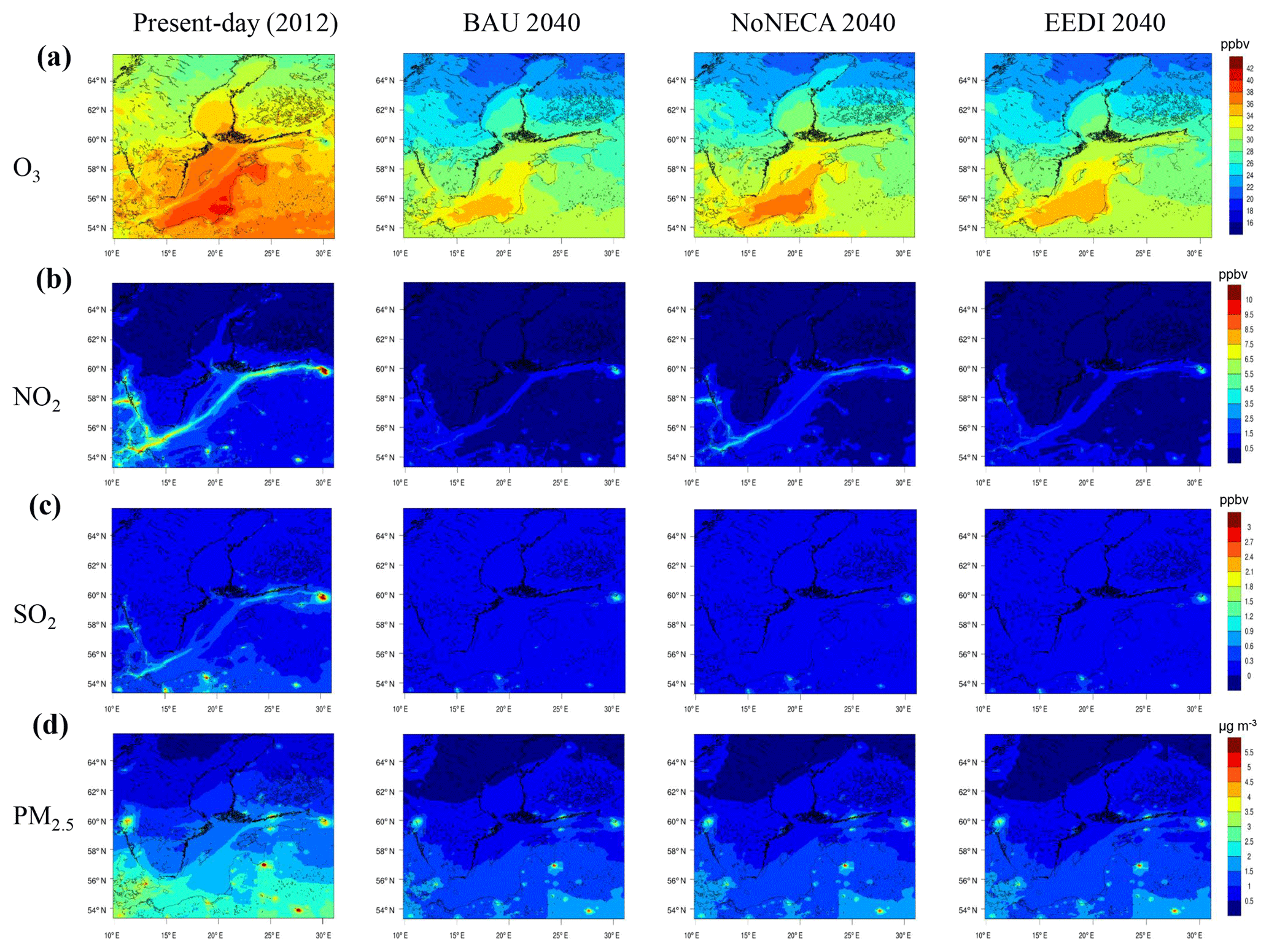
Figure 6Future air quality situation in the Baltic Sea region in summer (JJA) compared to the present day. CMAQ model results for present-day (first column), for BAU 2040 (second column), for NoNECA 2040 (third column) and for EEDI 2040 (fourth column) are shown for (a) daily maximum O3, (b) NO2, (c) SO2 and (d) PM2.5.
Over most parts of the Baltic Sea region, the summer mean of daily maximum O3 in BAU 2040 decreases by 10 %–25 % compared to 2012, as a consequence of the NECA and reduced land-based emissions of NOx (Fig. 6a). The future change in ozone is similar in EEDI 2040, implying that the effect of increased fuel efficiency is less pronounced and that the NOx reduction through establishing the NECA has a much greater influence on future ozone levels in the Baltic Sea region. In the NoNECA scenario, daily maximum O3 over land will decrease less than in the BAU scenario, but still an average ozone reduction by 15 % in 2040 is predicted for large parts of Sweden and the Baltic Sea compared to the present day.
In the BAU 2040 scenario, summer mean NO2 concentrations are drastically reduced by ∼80 % over most parts of the Baltic Sea and by up to ca. 90 % in the northern Baltic Proper compared to 2012 (Fig. 6b). This appears to be a result of the combined emission reductions through the NECA and the regulation of land-based emissions (Sect. 3.3), leading to a shift in the overall atmospheric photochemical regime due to the lower abundance of NOx in the future. A strong reduction is also seen in EEDI 2040, where NO2 levels over the Baltic Sea decrease by ∼80 % compared to 2012. NoNECA 2040 results in a reduction in NO2 by ∼50 % over the entire Baltic Sea.
BAU 2040 adopts the agreed SOx emission reduction measures; i.e. the SECA limit of 0.1 % S in fuel from 2015 onwards and the global limit of 0.5 % S in fuel from 2020 onwards. The other two future scenarios also implement the two sulfur regulations. In 2040, summer mean SO2 levels drop by 80 %–90 % over the entire Baltic Sea compared to the present day.
Summer mean PM2.5 levels in 2040 decrease by 50 %–60 % along the main shipping routes and by 40 %–50 % in the other parts of the Baltic Sea compared to 2012. The EEDI scenario involves lower primary PM emission reductions (by 51 %) than in BAU 2040 and NoNECA 2040 (by 65 %). However, as for the other air pollutants, no large differences in the spatial concentration distributions in summer 2040 are seen between the EEDI and the BAU scenarios, suggesting that the lower fuel efficiency increase has only marginal implications on the future air quality in the Baltic Sea region.
5.1.2 Influence of ship emissions in the BAU future scenario
Figure 7 summarizes the predicted ship contribution in summer 2040 according to the BAU 2040 scenario, which is analogous to Fig. 5 for the present-day ship contribution. As a result of the introduction of the NECA in 2021, the future impact of ship emissions on O3 levels in the Baltic Sea region diminishes. In 2040, the ship contribution to summer mean daily maximum O3 concentrations is highest over the Gotland Basin (range: 5–6 ppbv), while it is smaller for all over parts of the Baltic Sea region, not exceeding 4.5 ppbv. Overall, the model simulations predict that shipping emissions will still influence ozone levels over the Baltic Sea and in the coastal areas in 2040, with relative contributions in the range of 10 %–20 % to daily maximum O3.
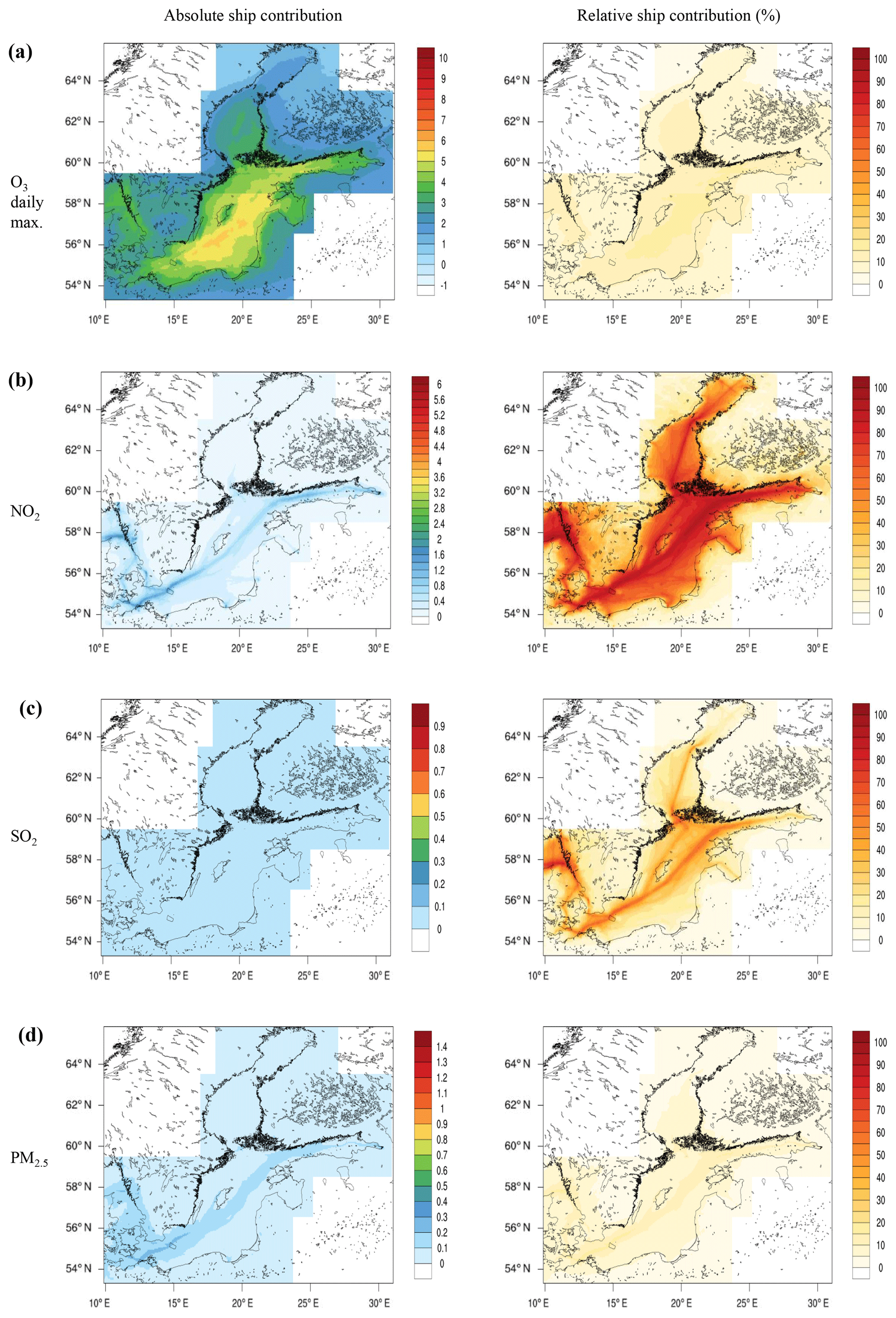
Figure 7Future (2040) ship contribution in the Baltic Sea region in summer (JJA) from CMAQ model results for the BAU 2040 scenario: ship-related concentration (left) for gaseous pollutants (in ppbv) and for PM2.5 (in µg m−3), percentage ship contribution (right) for (a) daily maximum O3, (b) NO2, (c) SO2, and (d) PM2.5. Ship-related contribution only shown for the high-resolution area. The same scales as in Fig. 5 were used to facilitate comparison of the concentration and contribution maps. The sharp change in the O3 ship contribution north of 58.8∘ N is an artefact of the averaging in the overlap area of the two 4 km resolution grids.
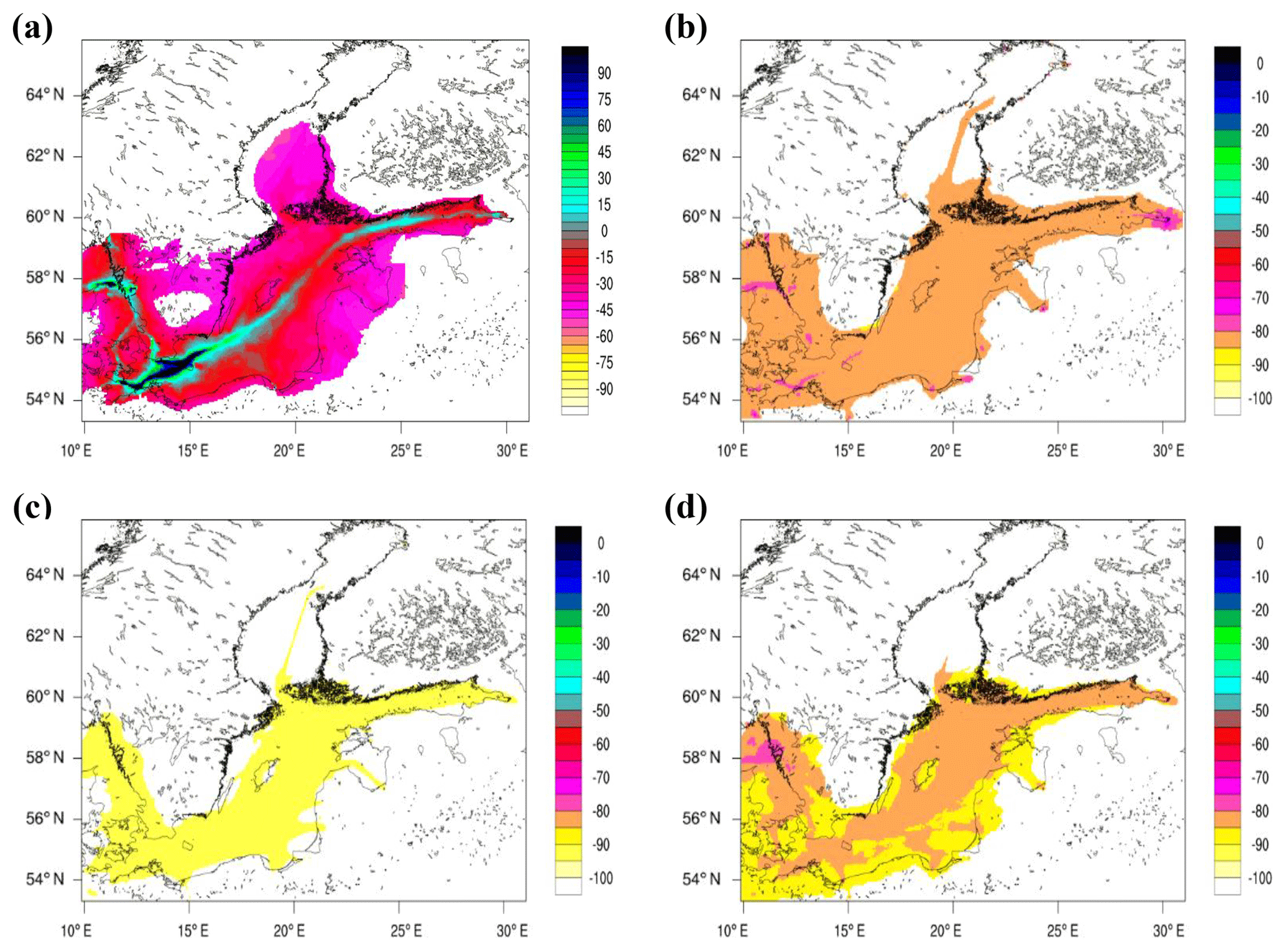
Figure 8Future (2040) change in the ship-related contribution in summer (JJA) in percent compared to 2012, given as the relative difference between the ship contribution from the BAU 2040 simulation and the ship contribution from the present-day simulation: (a) daily maximum O3, (b) NO2, (c) SO2 and (d) PM2.5. Not coloured (empty) areas indicate grid cells with a ship contribution in BAU 2040 of less than 1.0 ppbv, 0.1 ppbv, 0.01 ppbv and 0.005 µg m−3, for daily max O3, NO2, SO2 and PM2.5, respectively. Ship-related contribution only shown for the high-resolution area. Note the different scale for daily max O3 (from −100 % to 100 %).
The absolute ship contribution to summer mean NO2 concentrations in 2040 drops substantially compared to 2012. The ship-related NO2 concentration decreases from ca. 3 ppbv in the present-day situation to 0.5–1.5 ppbv in the BAU scenario, along the main shipping routes. Even with the NECA established, emissions from ship traffic remain the dominant contributor to atmospheric NO2 over the Baltic Sea in 2040.
The absolute ship contribution to SO2 concentrations in summer 2040 is less than 0.1 ppbv. However, the ship influence on ambient SO2 concentrations has not completely vanished in 2040. Along the main shipping routes throughout the Baltic Sea, the relative contribution remains high.
The absolute ship contribution to PM2.5 in summer 2040 is predicted to be ≤0.2 µg m−3 over most parts of the Baltic Sea region, with higher values over the Belt and Kattegat (0.4 µg m−3). The ship influence is substantially weakened compared to the present-day situation: the relative contribution peaks along the shipping routes (15 %–25 %) and is below 10 % over land.
5.1.3 Future change in the ship contribution
Figure 8 shows the future change in the ship contribution in summer 2040 compared to 2012 when following the BAU 2040 scenario. Future changes in the ship contribution to daily maximum O3 are divided into two regions with opposing signs, one with a relative increase over the central shipping routes, and one with a relative decrease outside the ship tracks and over the coastal regions. Over the ship lanes, ozone recovers due to reduced titration of ozone in the ship plumes following the lower emissions of NO from ships. At a greater distance from the ship lanes, photochemical production of ozone declines compared to the present day, giving rise to lower O3 concentrations.
The ship contribution to NO2 decreases by 80 %–85 % over the Baltic Sea, but is slightly more than linear with the reduced NOx emissions from shipping. The decrease is smaller (∼77 %) in some port cities like Gdansk and St Petersburg and in areas with a high density of ship traffic. The reduced NOx emission from ships causes an increase in the ratio of [NO2] to [NO] (short: NO2-to-NO ratio) in the ship plumes. Although the NO2-to-NO ratio at the ship stack is the same (equal to 5 : 95), it becomes higher, as NO2 from the background air entrains into the plume, than in the present-day situation. According to the photostationary state relation, the increased ratio causes a higher steady-state O3 concentration in the ship plume. With the local increase in O3, the reaction of NO with the hydroperoxyl (HO2) radical giving NO2 starts to compete with the titration reaction (reaction of NO with O3). In the reaction of NO with HO2 an additional ozone molecule is produced, as the resulting NO2 molecule photolyses, amplifying the ozone production in the plume. Hence the smaller decrease in the NO2 ship contribution is due a change in the photochemistry regime in the ship plumes accompanied with a higher conversion of NO to NO2.
For the ship contribution to SO2, a uniform decline of around 90 % is seen for the entire Baltic Sea in accordance with a linear decrease following the reduction in SOx emissions from shipping of 91.2 % between 2012 and 2040 in BAU 2040. Note that ship emissions of SOx were attributed completely to SO2. As for the NO2 ship contribution, the decrease is slightly higher than expected due to the reduction in ship emissions. Due to the drastic decrease in nitrogen oxides, the atmospheric oxidation capacity increases in the future scenario simulation, leading to more efficient oxidation of pollutants and higher availability of photo-oxidants (OH and HO2 radicals). Hence, the removal rates of SO2 and NO2 by reaction with photo-oxidants and the rate of SO2 oxidation in clouds are slightly increased in 2040 compared to 2012.
The ship-contributed summer mean PM2.5 between 2012 and 2040 (BAU 2040) is reduced by 75 %–90 %, with largest reductions over the southern part of the Baltic Sea and in the coastal regions. This is more than can be explained by the reduction in primary PM emissions (by 65 %) from shipping. Thus a substantial fraction of the changed ship contribution is caused by changes in the secondary aerosol production. The future ship contribution to PM2.5 is affected by reduced SOx emissions from ships, as a result of the regulations for lower sulfur fuel content and by reduced NOx emissions due to the NECA.
Together, the regulations lead to a decline in the atmospheric formation of sulfate and nitrate particles related to shipping. In the southern part of the Baltic Sea region, especially over Denmark and northern Germany, the ship-related formation of secondary aerosol is also affected by the lower NH3 emissions from agriculture. Decreasing atmospheric ammonia concentrations reduce the formation of ammonium nitrate particles, since their formation is limited by the availability of NH3.
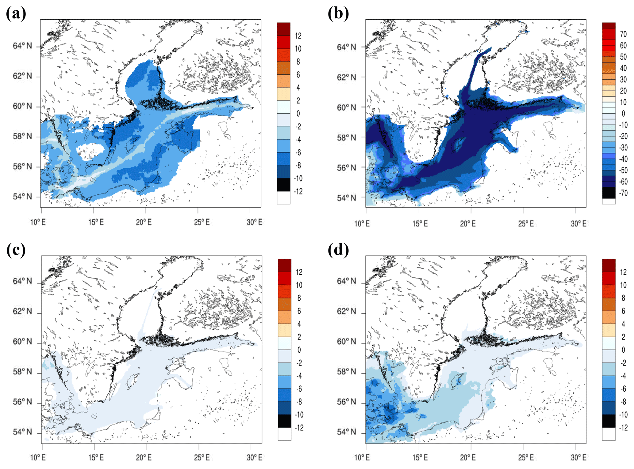
Figure 9Effect of establishing the NECA (in 2021) on the future air quality in summer (JJA) 2040 in the Baltic Sea region as relative difference (in percent) between the scenario simulations BAU 2040 and NoNECA 2040: (a) daily maximum O3, (b) NO2, (c) SO2 and (d) PM2.5. Not coloured (white) areas indicate grid cells with ship contribution in BAU 2040 of less than 1.0 ppbv, 0.1 ppbv, 0.01 ppbv and 0.005 µg m−3, for daily max O3, NO2, SO2 and PM2.5, respectively.
For the other two future scenarios, NoNECA 2040 and EEDI 2040, changes in the ship-contributed pollutant concentrations compared to the present day are smaller than in BAU 2040. In the scenario without the implementation of NECA, NoNECA 2040, the ship contribution to NO2 in 2040 decreases by 50 %–60 % over the Baltic Sea (Fig. S13). The ship contribution to ozone increases widely by more than 10 % compared to the present day, indicating enhanced ozone production due to shipping activities in 2040, mainly over sea and the coastal areas of Sweden, Denmark and Poland. The EEDI scenario, with lower fuel efficiency, results in a significantly smaller reduction in ship-contributed PM2.5 than the BAU scenario. Still, the ship-contributed summer mean PM2.5 between 2012 and 2040 is reduced by 65 %–80 % over the impacted areas (Fig. S14).
5.2 Future air quality: effect of the NECA
The difference between the two future scenarios BAU 2040 and NoNECA 2040 is the higher emission reduction in NOx from shipping in the BAU scenario through the establishment of the NECA. Figure 9 illustrates the effect of introducing the NECA in 2021 into major air quality components compared to a future situation without NECA, determined based on the difference between modelled concentrations in the BAU 2040 and NoNECA 2040 scenarios. Land-based emissions are the same in both scenarios; therefore changes are solely due to different ship emissions in the two future scenarios.
The result of the NECA in 2040 is a reduction in NOx emissions from shipping by 59 % on average, corresponding to the difference between a Tier 3-dominated ship fleet with the NECA and Tier 2-dominated ship fleet without the NECA. The reduction in NOx emissions from shipping primarily translates into a ∼60 % decrease in NO2 summer mean concentrations within a wide corridor of the ship routes. In addition, the population in coastal areas in northern Germany, Denmark and western Sweden will be less exposed to NO2 in 2040 due to the introduction of the NECA. Due to the lower atmospheric NOx levels, less ozone is formed, and daily maximum O3 concentration over the Baltic Sea in summer 2040 is on average 6 % lower than without the NECA. In the areas close to the main shipping routes, ozone is almost unchanged despite the sharp reduction in NOx emissions, probably due to compensating effects between changed titration losses and changed photochemical ozone production. As expected, levels of atmospheric SO2 are largely unaffected by the NECA ( %).

Figure 10Effect of lower fuel efficiency on the future air quality in summer (JJA) 2040 in the Baltic Sea region as relative difference (in percent) between the scenario simulations EEDI 2040 and BAU 2040: (a) daily maximum O3, (b) NO2, (c) SO2 and (d) PM2.5. Not coloured (white) areas indicate grid cells with ship contribution in BAU 2040 of less than 1.0 ppbv, 0.1 ppbv, 0.01 ppbv, 0.005 µg m−3, for daily max O3, NO2, SO2 and PM2.5, respectively.
A secondary effect of the NECA is a reduction in the formation of particulate nitrate. Due to the non-linearity of the atmospheric particle mass formation (i.e. photochemistry and gas-to-particle conversion depend on precursor concentrations and existing particulate matter in a non-linear fashion) the impact of reducing gaseous precursors does not result in a linear reduction in future PM2.5 levels. Figure 9d shows the change in summer mean PM2.5 concentration pattern due to the NECA. Note that primary emissions of PM2.5 are the same in BAU and NoNECA; thus changes are solely attributed to modified particulate nitrate concentrations. The largest decrease in PM2.5, by up to 8 %, occurs over the Danish islands, where the abundance of ammonium nitrate is highest.
5.3 Future air quality: effect of lower fuel efficiency
The BAU scenario assumes an improvement in the marine fuel efficiency beyond that required by the EEDI regulation for new ships. With the difference between the EEDI 2040 and BAU 2040 scenarios (land-based emissions are the same in both scenarios), the effect of a slower rate of fuel efficiency improvement compared to the projections in the BAU scenario on the air quality in 2040 is determined. The lower fuel efficiency affects the ship engine emissions and leads to NOx, SO2 and PM2.5 emissions from ships that are on average 37.9 %, 36.8 % and 39.6 % higher in 2040, respectively, compared to the BAU scenario. As a consequence of the lower fuel efficiency, modelled summer mean concentrations of NO2 and SO2 along the main shipping routes in 2040 are higher by 40 % and 25 % than in BAU, respectively (Fig. 10).
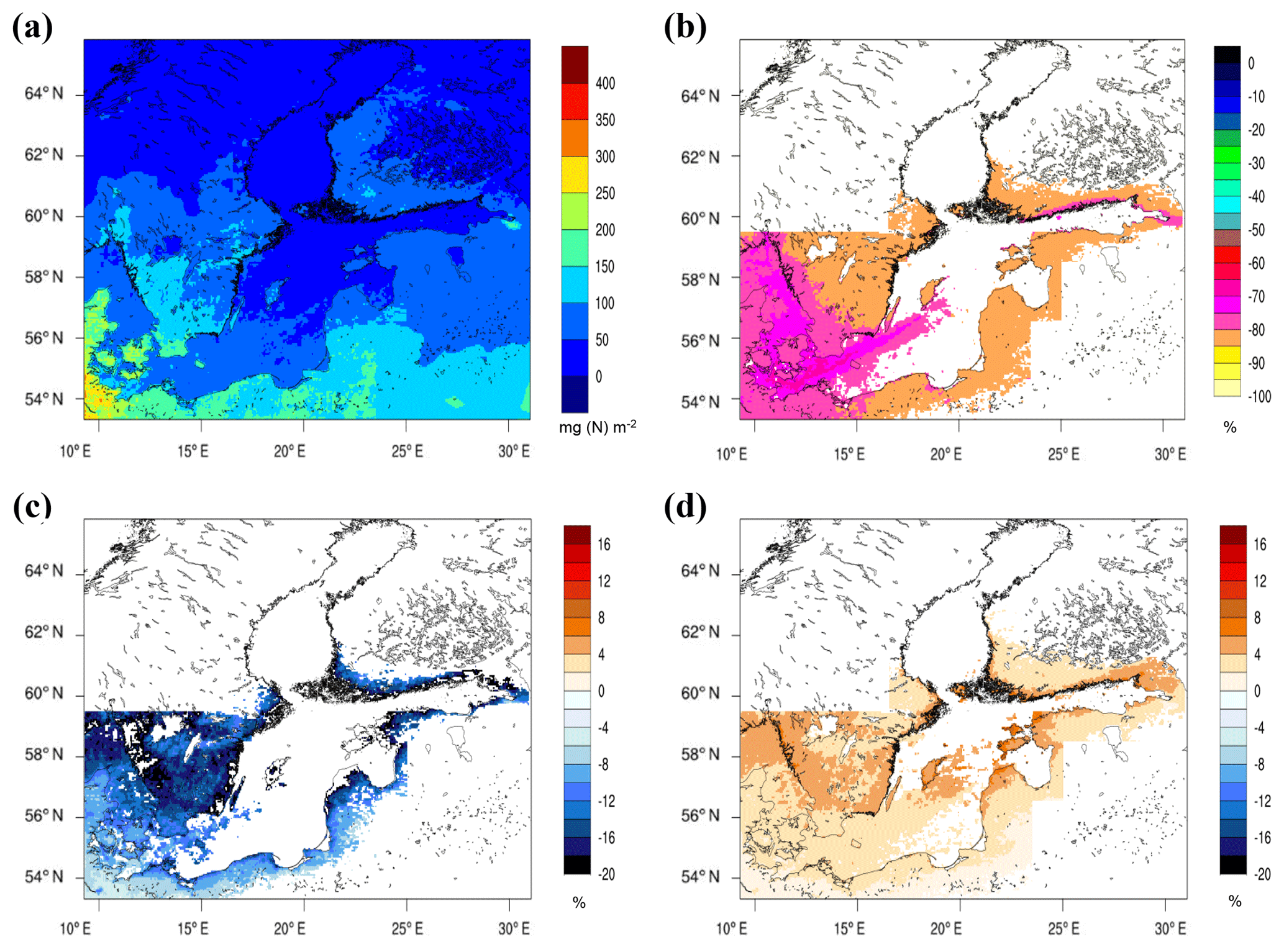
Figure 11Nitrogen deposition in summer (JJA) 2040: (a) accumulated total deposition of nitrogen (in mg(N) m−2) in scenario BAU 2040, (b) percentage change in the ship contribution to nitrogen deposition in scenario BAU 2040 compared to the present day, (c) effect of the NECA on nitrogen deposition, and (d) effect of the lower efficiency of EEDI on nitrogen deposition. Not coloured (empty) areas indicate grid cells with ship contribution in BAU 2040 of less than 6.0 mg(N) m−2 for total nitrogen deposition. The ship-related contribution is only shown for the high-resolution area.
The lower fuel efficiency has little influence on daily maximum ozone concentrations over the Baltic Sea. Further, the influence of the changed fuel efficiency on atmospheric secondary particle formation is rather limited (not shown). For PM2.5, the higher primary particle emissions compared to BAU do not fully propagate into surface air concentrations (increase by less than 10 %). A large fraction of the ship-related PM2.5 is from secondary formation, which does not increase proportionally with the increased primary PM emissions, for example due to the limited availability of NH3.
5.4 Future nitrogen deposition
Summer-accumulated total nitrogen deposition to seawater in 2040 according to BAU 2040 is below 100 mg(N) m−2 in most parts of the Baltic Sea, with highest deposition remaining in the Belt Sea (Fig. 11a). The average summer deposition rate for the Baltic Sea is 48 mg(N) m−2. The ship contribution to total nitrogen deposition in summer is massively reduced (by more than 60 %) in the coastal areas of the Baltic Sea region compared to 2012 (Fig. 11b). Over sea, largest reductions of the ship contribution take place in an area extending from Kattegat to the Arkona basin.
Table 4Future (2040) annual and seasonal nitrogen deposition amounts (kt N) to the seawater of the Baltic Sea and ship-related nitrogen deposition according to scenario BAU 2040, taken from the CD04 grid. Values in brackets denote the change (in kt N) compared to 2012. Amounts refer to a Baltic Sea surface area of 431 390 km2, including the western part of Skagerrak.
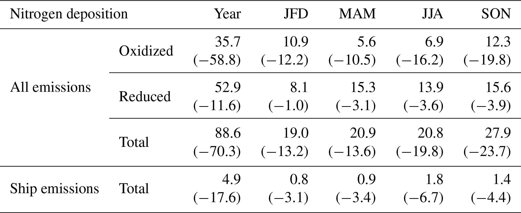
The introduction of the NECA causes a maximum reduction in the summer-accumulated nitrogen over seawater by 18 % compared to not introducing the NECA in 2021 (Fig. 11c). This means that the Tier 2 fleet in NoNECA 2040 already accomplishes a large reduction in nitrogen deposition compared to today. The effect of the lower fuel efficiency in 2040 (according to EEDI 2040) is an increase in nitrogen deposition compared to BAU, mainly over the northern Baltic Proper and over coastal areas. The relative increase is up to 12 % (Fig. 11d).
Table 4 shows the BAU 2040 annual and seasonal nitrogen deposition sums to the entire Baltic Sea seawater surface, for total, oxidized and reduced nitrogen. The ship-related annual nitrogen deposition is reduced by 17.6 kt N, while the overall nitrogen deposition is reduced by 70.3 kt N compared to 2012. Thus the reduction in NOx emissions over the continent, in accordance with a current legislation scenario for land-based emissions in the Baltic Sea region, has a larger impact on the future nitrogen input to the Baltic Sea than the shipping fleet.
6.1 Changes in the air quality in the future scenarios
In the BAU scenario, with the introduction of the NECA in 2021, NOx emissions from ship traffic in the Baltic Sea are reduced by about 80 % in 2040 because most ships of the Baltic Sea ship fleet will then fulfil the Tier 3 regulation. With the NoNECA scenario, the entire ship fleet follows Tier 2 regulations for NOx in 2040 and, in conjunction with the fuel efficiency increase, leads to an overall NOx emission reduction from the ship fleet by about 50 %.
Table 5 presents the relative changes in annual mean concentrations of air pollutants in the Baltic Sea region between 2012 and 2040 (as average of the CD04 grid domains). Annual mean NO2 decreases by 61 %–72 % between 2012 and 2040 in the Baltic Sea region, depending on the shipping scenario, with the smallest decrease in the NoNECA scenario.
The BAU scenario adopts the agreed SOx emission abatement regulations: the pre-established SECA limit of 0.1 % S in fuel from 2015 onwards followed by the global limit of 0.5 % S in ship fuels from 2020 onwards. On average, annual mean SO2 decreases by ∼60 % between 2012 and 2040, independent of the shipping scenario. Consequently, particulate sulfate decreases by 50 %–60 % over the Baltic Sea between 2012 and 2040 (not shown) in all three scenarios. The burden of PM2.5 over the Baltic Sea region decreases by 35 %–37 % between 2012 and 2040 (Table 5). The reduction in PM2.5 is larger over sea, where it drops by 50 %–60 % along the main shipping routes, and is smaller over the coastal areas. The large drop over sea is due to the reduction in particulate matter emissions from ships and the lower production of sulfate and nitrate related to reduced emissions of primary precursor gases (NOx and SOx) from ship traffic. In most coastal areas the decreased PM2.5 is mainly a consequence of the abatement measures on land.
Table 5Summary of overall changes in future scenarios. Changes (in percent) in spatial average for all future scenarios compared to the present day (simulations with all emissions): annual means of NO2, SO2, PM2.5 and the daily maximum O3 within the 4 km resolution area (CD04 grid domains) and annual sum of nitrogen deposition to seawater.
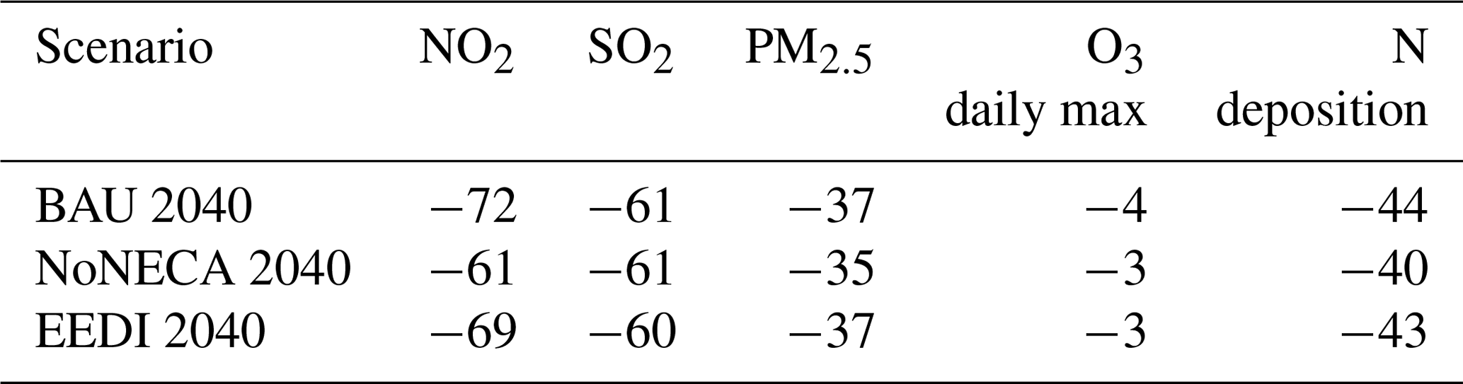
On an annual average, the daily maximum O3 decreases only slightly over the Baltic Sea region, but the summer average decreases by 10 %–25 %, depending on the shipping scenario, in large parts of Sweden and the Baltic Sea compared to the present day.
Overall, a lower fuel efficiency increase than in BAU has only marginal implications on the future air quality in the Baltic Sea region.
6.2 Changes in the ship contribution in the future scenarios
The absolute ship contribution to ambient levels of NO2 and SO2 between 2012 and 2040 changes slightly more than expected due to the reduction in ship emissions. The lower abundance of NOx in the future atmospheric background increases the oxidation capacity of the atmosphere and leads to more efficient oxidation of pollutants via gas-phase reactions and in-cloud processing. Table 6 presents the relative changes in the annual mean absolute ship contributions in the Baltic Sea region between 2012 and 2040.
A consequence of establishing the NECA is the reduction in the ship contribution to daily maximum ozone by 18 % on average compared to the present situation. If the NECA is not implemented, an increase in the ship-related daily maximum ozone by 31 % results compared to the present day. The introduction of NECA is hence critical for abating ship emissions of NOx to levels that are low enough to sustainably dampen ozone production in the Baltic Sea region. A second important effect of the NECA over the Baltic Sea region is a reduction in secondary formation of particulate nitrate. The introduction of the NECA reduces the ship-related PM2.5 by 72 % in 2040 compared to the present day, while it is reduced by only 48 % without implementation of the NECA.
The effect of the lower fuel efficiency on the absolute ship contribution of air pollutants is limited. Still, the annual mean ship contributions in 2040 to the four pollutants are significantly higher than in the BAU scenario.
Table 6Summary of ship contribution changes in future scenarios. Changes (in percent) in spatial average of the ship contributions for all future scenarios compared to the present day (simulations with all emissions): annual means of NO2, SO2, PM2.5 and the daily maximum O3 within the 4 km resolution area (CD04 grid domains) and annual sum of nitrogen deposition to seawater.
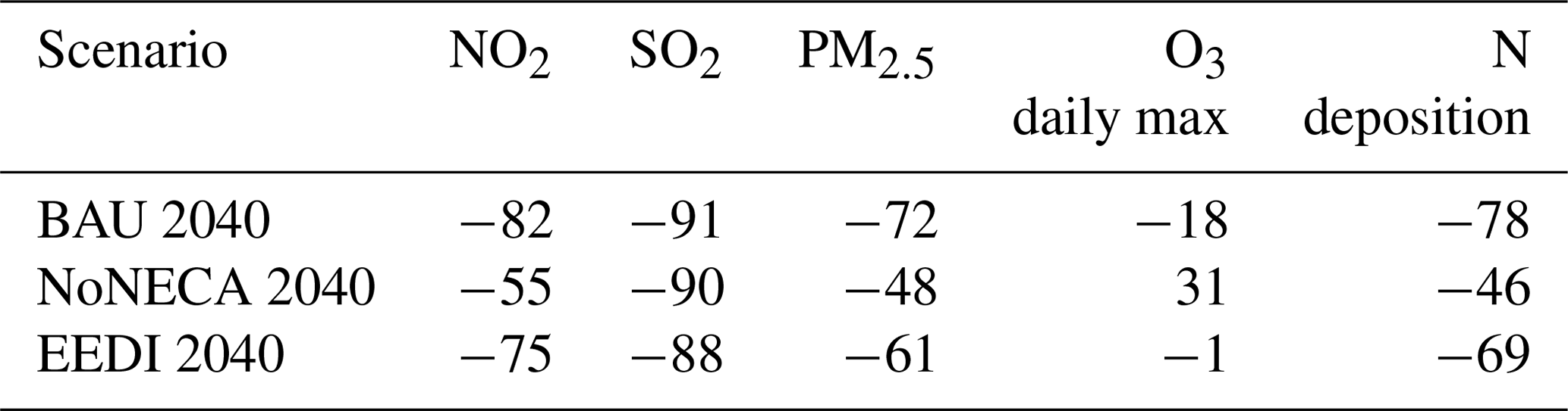
6.3 Contribution of ship emissions to nitrogen deposition
A previous study (Bartnicki et al., 2011) estimated the contribution of airborne nitrogen from international ship traffic to the oxidized nitrogen deposition in the Baltic Sea basin to be about 8 % to 11 % (period: 1997–2006) on an annual average. The contribution from ships with a range from 12 % to 14 % has been reported for the period 2008 to 2011 (Hongisto, 2014). In the present study, the relative ship contribution to the deposition of oxidized nitrogen is 24 % (Table 3), about twice as high as the previous estimates. However, the total annual nitrogen deposition for 2012 in the present study is 29 % lower compared to the EMEP MSC-W model used by HELCOM (Bartnicki et al., 2017). Taking the literature value of 14 % and the oxidized nitrogen deposition flux in 2012 reported by HELCOM (128.9 kt N yr−1; Bartnicki et al., 2017), an absolute ship contribution of 18 kt N yr−1 is derived, which is only slightly lower than our estimate of 22.5 kt N yr−1.
The relative ship contribution to the total nitrogen deposition is 14 % on annual average and 21 % in summer in the present-day situation (Table 3). The ship contribution drops to 5.6 % in 2040 (9 % in summer) when following the BAU scenario (Table 4). Between 2040 and 2012 the ship-related deposition of oxidized nitrogen decreased by 78 %. In BAU 2040 the ship contribution to the annual deposition of oxidized nitrogen over the Baltic Sea is only 14 %.
Nitrogen deposition to the seawater of the Baltic Sea decreases on average by 40 %–44 % between 2012 and 2040 (Table 5). Depending on the future shipping scenario, the decline in the ship-related nitrogen deposition varies between 46 % and 78 % (Table 6). In the EEDI scenario, when the NECA is established but fuel efficiency increase is lower than in BAU, nitrogen deposition in most ship-influenced areas decreases less than in the BAU scenario. The weakest reduction is found for the NoNECA scenario, in which nitrogen deposition decreases by only 30 % over coastal areas of Denmark, Germany and western Finland. The western part of the Baltic Sea would be most affected if the NECA is not implemented (Fig. 11c).
6.4 Prognosis of the total nitrogen deposition to the Baltic Sea
A linear relationship was found between the emissions of NOx from the Baltic Sea ship fleet and the annual ship-related nitrogen deposition to Baltic Sea seawater (spatial average) based on the results of the present-day simulation and the future scenario simulations (Fig. 12). Because the changes in the nitrogen deposition attributed to shipping (Fig. 11b) between 2012 and 2040 are mainly confined to the Baltic Sea and the surrounding coastal areas, it was expected that the changes in the ship-related deposition flux are proportional to the atmospheric input of oxidized nitrogen via ship emissions. An important link between the ship emissions and the deposition of nitrogen is the formation of HNO3, which constitutes the most important removal pathway for nitrogen in the atmosphere (Riemer et al., 2003).
The relationship presented above is useful for a quick evaluation of the ship-related nitrogen deposition in future shipping scenarios. Cumulative scenarios based on Shared Socioeconomic Pathways (SSPs) with respect to future ship emission in the Baltic Sea region were designed in the SHEBA project. In scenario SSP3 (regional rivalry), which represents a world with much less international trade and low mitigation capacity (Fujimori et al., 2017), future shipping deviates largely from the predefined regulations but growth of shipping is slower than in BAU by 0.5 % yr−1. The fuel efficiency development is lower by 1 % yr−1 than in EEDI. Use of LNG is similar as in BAU. The Tier 2 regulation is not enforced in SSP3; i.e. the entire ship fleet applies the Tier 1 standard for NOx emissions. Ship NOx emissions in SSP3 are 143 kt N yr−1, somewhat lower than in the current situation. Based on the linear model the ship-related nitrogen deposition is estimated to be 21.5 kt N yr−1.
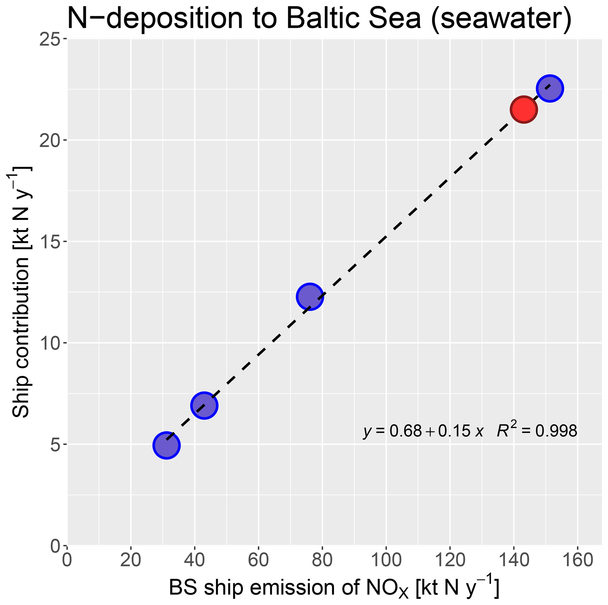
Figure 12Relationship between emissions of NOx (in kt N yr−1) from the Baltic Sea ship fleet and the annual ship-related nitrogen deposition (in kt N yr−1) to the Baltic seawater (on spatial average) based on the model results of the present-day simulation and the model results of the future scenario simulations. Red-filled circle indicates the ship contribution in scenario SSP3 predicted from the linear fit to the relationship.
Thus, in this quick assessment, SSP3 brings a slight improvement in 2040 compared to the current situation. The comparison of the simulated future scenarios to SSP3 also underlines the potential of the Tier 2 standard regulation for newly built ships (as in NoNECA 2040) to reduce the future impact from shipping, compensating, together with the faster fuel efficiency development, the projected higher ship traffic growth.
6.5 Discussion of uncertainties and limitations
The ship contribution to air pollutants and nitrogen deposition in the present study was computed using a zero-out method; i.e. the ship emissions were removed in one simulation. An alternative brute-force method would be the perturbation of the emissions, for example reduction by 20 %, which might be more careful with respect to the non-linearity of the involved photochemistry. However, our goal was to derive the impact of shipping in different scenarios, while perturbing emissions is mainly used to investigate short-term responses to expected (small) changes in a sectoral emissions. A previous study by Geels et al. (2012) applied the so-called tagging method to assess the ship contribution from each riparian state of the Baltic Sea. Tagging requires adding auxiliary variables to the CTM itself to track pollution. While tagging for inert primary pollutants is straightforward; methods for addressing secondary pollutants require an analysis of the limiting reagents to avoid tagging all possible follow-up products in the gas-phase, aerosol phase and cloud water. Differences between tagging and brute-force methods are usually observed in secondary processes involving precursors from different sources. Some comparison studies (Collet et al., 2014; Koo et al., 2009) indicate that tagging is advantageous for source allocation rather than for predicting responses to emissions changes.
European regions that are affected by a high density of ship traffic, such as the UK, France, western Germany, North Sea, the southern part of the Baltic Sea and along the ship tracks in the Mediterranean, are currently in a NMVOC-limited regime with respect to ozone formation (Beekmann and Vautard, 2010). In northern Europe, except for the region of the English Channel and parts of the North Sea, a transition from NMVOC-limited to NOx-limited regime is projected until 2020 (Beekmann and Vautard, 2010) and the next decades (Lacressonnière et al., 2014). In a NMVOC-limited regime the production of ozone is sensitive to emissions of NMVOC, while increasing NOx leads to a reduction in ozone by titration. In the NOx-limited regime, ozone is sensitive to emissions of NOx, while it is hardly affected by additional NMVOC emissions.
In the simulations for the future scenarios in 2040, a transition towards a NOx-limited regime most certainly happens in the currently NMVOC-limited areas of the Baltic Sea, in particular along the ship tracks in the southern part. This is clearly seen in the BAU 2040 scenario, where a relative increase in the ship-related daily maximum ozone occurred (due to less titration) over the central shipping routes, whereas the ship-related ozone decreased in the NOx-limited areas outside the ship tracks and over the coastal regions. However, predicted changes in the daily maximum ozone concentrations due to shipping are uncertain because of the lack of data on NMVOC emissions from shipping in the STEAM inventory that were used in the CTM calculations.
We have reduced land-based emissions in the future scenarios in order to obtain a more realistic estimation of the consequences of regulations on shipping emissions on the future air quality in the Baltic Sea region. Based on the model results for the future ship contribution, it is obvious that reduced land-side emissions of primary gaseous precursors amplified the decline in secondary aerosols related to shipping, in particular over the coastal areas. However, the reduction in land-side emissions has a very small effect on the determined ship contributions to NO2 and SO2 over the Baltic Sea (Fig. S15).
The reason for the underestimation of WNO3 and WNH4 in the CMAQ simulations compared to observations of the regional background monitoring stations of the EMEP network, could not be fully resolved. The formation of particulate nitrate involves complex chemistry of several compounds in the gas-phase and multi-component solution systems on aerosols. The simulation of nitrate is highly uncertain because it requires accurate computation of the concentrations of the precursors, e.g. HNO3, NH3, dust and sea salt. The joint underestimation of WNO3 and WNH4 was found in the statistical analysis of model–observation pairs and also in the comparison of modelled and observed seasonal averages. The most convincing explanation at the current stage is that the oxidative conversion of NOx to HNO3 occurs at a too-slow rate in the model, combined with too little particulate ammonium from the regional background that is advected into the Baltic Sea region.
An alternative explanation might be that the wet removal of and in CMAQ is not efficient enough. In addition, the evaluation of simulated precipitation amounts and frequency showed that the southern part of the Baltic Sea receives too little rainfall in summer. For the other seasons and in the northern part the precipitation bias is positive. Too-low precipitation in the southern part, where modelled concentrations of and are much higher compared to the northern part, could be responsible for an average underestimation of the total nitrogen wet deposition to the Baltic Sea.
Coarse-mode particles are removed much faster than fine-mode particles; therefore the deposition of particulate nitrate crucially depends on the uptake to larger particles. Heterogeneous chemical production of nitrate on coarse-mode particles has been found to control the atmospheric nitrate production to a very large extent (Bian et al., 2017). The hydrolysis of N2O5 to produce HNO3 is considered in CMAQ by uptake coefficients depending on temperature, RH and particle composition, using the parameterization by Davis et al. (2008), but only for fine-mode aerosols. The Davis parameterization tends to predict too-high N2O5 uptake coefficients near the surface, especially over marine and coastal areas, where relative humidity is high (Chang et al., 2016). CMAQ allows for dynamic mass transfer to coarse particles and therefore takes into account the reactive uptake of HNO3 by sea salt particles. Meanwhile, resuspension of mineral dust was not activated in the simulations, and the missing heterogeneous reaction on dust particles surfaces may have contributed to the underestimation of WNO3.
The impact of ship emissions on the present-day (2012) and future (2040) air quality and nitrogen deposition was evaluated with a regional atmospheric CTM. The meteorological fields, the emissions from ship traffic and the emissions from land-based sources are considered at a grid resolution of 4×4 km2 for the innermost model domain covering most of the Baltic Sea region. Ship emissions from the STEAM model based on ship movements from AIS records and detailed ship characteristics in combination with solving atmospheric chemistry and transport at high resolution, enable a better treatment of the plumes from ship traffic compared to previous CTM studies in the Baltic Sea region.
The effect of future legislation related to shipping and of future changes in the ship fuel efficiency of the ship fleet on air quality and deposition in 2040 in the Baltic Sea region was determined based on computational results from regional CTM simulations. Future air quality and nitrogen deposition is analysed in order to investigate (1) the effect of establishing the NECA in 2021 compared to a future situation without NECA and (2) the effect of a lower fuel efficiency increase than expected based on continuation of the current trend. A BAU scenario has been designed in which the NECA is implemented and the fuel efficiency for new ships improves more than required by IMO′s Energy Efficiency Design Index regulation.
Establishing the NECA in 2021 has several benefits for the Baltic Sea environment. One important effect of the NECA is a reduction in secondary formation of particulate nitrate. The introduction of the NECA reduces the ship-related PM2.5 by 72 % in 2040 compared to the present day, while it is reduced by only 48 % without implementation of the NECA. A major consequence of establishing the NECA is a reduction in the ship contribution to daily maximum ozone in 2040 compared to the present situation. If the NECA is not implemented, an increase in the ship-related daily maximum ozone results compared to the present day. The introduction of NECA is thus critical for abating ship emissions of NOx to levels that are low enough to sustainably dampen ozone production in the Baltic Sea region. Overall, the introduction of the NECA is expected to be beneficial for avoiding future health impacts of ozone and PM2.5 in coastal areas of the southern part of the Baltic Sea region.
The effect of the lower fuel efficiency on the absolute ship contribution of air pollutants is relatively small. The implementation of the NECA in 2021 can be regarded as a safeguard for the case that the fuel efficiency increase falls below the projected trend.
The decline in the ship-related nitrogen deposition to the Baltic Sea between 2012 and 2040 varies between 46 % and 78 % in different future scenarios. When the NECA is established but the fuel efficiency increase is lower than expected, nitrogen deposition in most ship-influenced areas decreases less than in the BAU scenario. The weakest reduction is found for the scenario without implementing the NECA, in which nitrogen deposition decreases by only 30 % over coastal areas of Denmark, Germany and western Finland. The western part of the Baltic Sea would be most affected if the NECA is not implemented.
A prognostic relationship for a quick evaluation of the ship-related nitrogen deposition in future shipping scenarios was derived in this work. The relationship should be further modified to consider the interannual variability of atmospheric deposition due to changing meteorological conditions in order to allow for more robust projections of the ship-related nitrogen input to the Baltic Sea. However, it may be used for estimating possible exceedances of critical loads for eutrophying substances that are based on annual nitrogen inputs.
A limitation of the model results for regional surface concentrations of the daily maximum ozone concentrations over the Baltic Sea region is the lack of data on NMVOC emissions from shipping in the STEAM inventory that were used in the CTM calculations. Additional NMVOC emissions from shipping would serve as precursors of ozone and enhance photochemical ozone production in a NMVOC-limited regime. In the presented model simulations, NOx emissions from continental sources were reduced by 60 % between 2012 and 2040, following current legislation, i.e. predefined emission abatement regulations. The lower abundance of NOx in the future could lead to a shift in the overall atmospheric chemical regime. To predict more accurately how such change in the chemical regime will affect the future influence of ship emissions, a better handle on NMVOC emissions from ships and their future development would be important.
As a consequence of SOx emission abatement regulations for shipping, annual mean SO2 decreases on average by ∼60 % between 2012 and 2040, independently of the future scenario. With the reduction in SO2 emissions, less NH3 is required to neutralize the strong acid H2SO4. The excess NH3 is available for the formation of and in the particulate phase. According to Tsimpidi et al. (2008), the trend of future particulate concentrations depends on whether NOx or NH3 are the limiting gas-phase compounds for nitrate formation. Measurements in southern Sweden have shown that the concentrations of NH3 and HNO3 are too low to form pure solid or aqueous ammonium nitrate particles (Ferm, 1992). Thus, in a future background atmosphere over the Baltic Sea region, ambient levels of both gases might be too low for ammonium nitrate formation, and the fate of these gases would be the removal by dry and wet deposition. Meanwhile, the formulation of heterogeneous processes related to the production of nitrate is highly uncertain in the models, limiting the conclusions about the future transition in the nitrate formation regime.
Use of the presented model data for health impact assessment in the densely populated coastal areas of the Baltic Sea region is connected to uncertainties arising from limitations of the chosen grid resolution. Despite the fine spatial resolution of the innermost model grid, the concentration gradients between urban areas and their surroundings (urban increment) and within harbour cities are not adequately resolved by the simulations due to the large spatial and temporal variability of emissions in urban areas. Ideally, a grid length of 1 km should be chosen to resolve the urban increments (Schaap et al., 2015) in the coastal areas. However, a finer resolution raises the need for more accurate emission data in the urban areas, which is challenging because the compilation of urban emission inventories requires specific information for each emitting sector (Guevara et al., 2016).
A related study by Jutterström et al. (2019) assessed the extent of environmental damage related to shipping on the terrestrial ecosystems surrounding the Baltic Sea. Ecological impacts of air pollutants on land are evaluated in terms of critical load (CL) exceedance for eutrophication. Using the latest reported CL values for eutrophication together with the modelled deposition data of nitrogen for 2012 and the future scenarios for 2040 of the present study, Jutterström et al. (2019) find a significant improvement from 2012 to 2040. For the BAU scenario, the area where the CL (eutrophication) are exceeded due to ship-related nitrogen deposition decreased from about 20 % in 2012 to 5 % in 2040. If the NECA is not implemented, the exceeded area due to shipping is about 14 % in 2040, indicative of the relevance of the NECA for coastal ecosystems surrounding the Baltic Sea. We note that the use of gridded model data of dry deposition in the estimation of CL exceedances has limitations. In the model simulation, dry deposition to land surfaces is weighted for the different land use classes present in each grid cell. This might lead to an underestimation of the eutrophication risk for forests in a grid cell which includes other land uses, as the canopy resistance of forests is much higher than that of grassland or other low vegetation. The CMAQ deposition data are less affected by this problem due to the high resolution of the gridded data.
The shipping sector is an important contributor to atmospheric nitrogen deposition in the Baltic Sea. The present study estimates a deposition flux of oxidized nitrogen in the order of 22.5 kt N yr−1 due to shipping emissions for the year 2012, which is slightly higher than previous estimates (Hongisto, 2014; Bartnicki et al., 2017). Occurrences of high nutrient input to coastal waters have been suggested to cause short-term algal blooms (Spokes et al., 2000). On the other hand, a study in the Kattegat showed that direct nitrogen inputs through atmospheric deposition could not be linked to any summer algal bloom observation, probably because the atmospheric input is considerably diluted through mixing in the surface water layer (Carstensen et al., 2005). The incidence of harmful algal blooms in shallow coastal waters, which damage the health of humans and animals, has also been linked to atmospheric nitrogen inputs (Paerl, 1997). However, the relationships between high nutrient inputs and the development of harmful algal blooms are still not well understood (Anderson et al., 2002).
Much stricter regulations for NOx emissions from newly built ships will be enforced in 2021. It can be expected that significant emission reductions will be the consequence of these regulations; however, this requires that the exhaust gas cleaning technologies that will be implemented on board most the newly built ships work properly. From the experiences with Euro 4 and Euro 5 diesel cars that frequently emit much more NOx than allowed, the policy should pave the way for extended compliance control measures. Several techniques exist on how emissions from ships can be measured, including in situ observations at coastlines, ground-based remote-sensing techniques, sniffers on board aircraft or drones and sensors on board the ships. The best technology needs to be tested now in order to be prepared for the implementation of the NECA.
The COSMO-CLM precipitation data and the CMAQ data on air pollutant concentrations and nitrogen deposition are available upon request.
The supplement related to this article is available online at: https://doi.org/10.5194/acp-19-1721-2019-supplement.
MK designed the overall structure of the paper, led the writing and did most of the writing, prepared input data and performed simulations with CMAQ, programmed a framework for data processing, did the visualization and plotting of the results and evaluated the air concentrations and nitrogen deposition data. JB provided land-based emissions with SMOKE-EU and text contributions on present-day and future land-based emissions. BG performed COSMO-CLM model simulations, evaluated and visualized the precipitation data and contributed text to the meteorological modelling. VM developed the research questions, helped with organizing the manuscript and contributed to the text of the Conclusions. JPJ and LJ were involved in the design of future scenarios, provided shipping emissions with STEAM, and contributed text on shipping emissions. EF developed the future scenarios and contributed data and text on the scenarios.
The authors declare that they have no conflict of interest
This article is part of the special issue “Shipping and the Environment – From Regional to Global Perspectives (ACP/OS inter-journal SI)”. It is a result of the Shipping and the Environment – From Regional to Global Perspectives, Gothenburg, Sweden, 23–24 October 2017.
This work is part of the BONUS SHEBA (Sustainable Shipping and Environment of the Baltic Sea region) research project under Call 2014-41. BONUS (Art 185) is funded jointly by the EU and by the German Federal Ministry of Education and Research under grant number 03F0720A, Innovation Fund Denmark, Estonian Research Council, Academy of Finland, National Centre of Research and Development (Poland) and Swedish Environmental Protection Agency. The air quality model CMAQ is developed and maintained by the U.S. Environmental Protection Agency (US EPA). COSMO-CLM is the community model of the German climate research (https://www.clm-community.eu/, last access: 6 February 2019). The simulations with COSMO-CLM and CMAQ were performed at the German Climate Computing Centre (DKRZ) within the project “Regional Atmospheric Modelling” (project ID 0302). The Swedish Meteorological and Hydrological Institute (SMHI) is thanked for making available the precipitation data from rain gauge stations in Sweden.
Zbigniew Klimont (IIASA) is thanked for emission data for the 2040 CLE
scenario from ECLIPSE v5.
NILU is thanked for the EBAS database maintenance and data provision.
Sara Jutterström (IVL) is thanked for good collaboration and discussion of
model results on deposition of nitrogen and sulfur.
The article processing charges for this open-access
publication
were covered by a Research
Centre of the Helmholtz Association.
Edited by: Huan Liu
Reviewed by: Nicolas Moussiopoulos and one anonymous referee
Amann, M., Borken-Kleefeld, J., Cofala, J., Hettelingh, J.-P., Heyes, C., Höglund-Isaksson, L., Holland, M., Kiesewetter, G., Klimont, Z., Rafaj, P., Posch, M., Sander, R., Schöpp, W., Wagner, F., and Winiwarter, W.: The Final Policy Scenarios of the EU Clean Air Policy Package, TSAP Report #11, International Institute for Applied Systems Analysis, Laxenburg, Austria, 2014. a
Anderson, D. M., Glibert, P. M., and Burkholder, J. M.: Harmful algal blooms and eutrophication: Nutrient sources, composition, and consequences, Estuaries, 25, 704–726, https://doi.org/10.1007/BF02804901, 2002. a
Andersson-Sköld, Y. and Simpson, D.: Secondary organic aerosol formation in northern Europe: a model study, J. Geophys. Res., 106, 7357–7374, https://doi.org/10.1029/2000JD900656, 2001. a
Appel, K. W., Pouliot, G. A., Simon, H., Sarwar, G., Pye, H. O. T., Napelenok, S. L., Akhtar, F., and Roselle, S. J.: Evaluation of dust and trace metal estimates from the Community Multiscale Air Quality (CMAQ) model version 5.0, Geosci. Model Dev., 6, 883–899, https://doi.org/10.5194/gmd-6-883-2013, 2013. a, b
Appel, K. W., Napelenok, S. L., Foley, K. M., Pye, H. O. T., Hogrefe, C., Luecken, D. J., Bash, J. O., Roselle, S. J., Pleim, J. E., Foroutan, H., Hutzell, W. T., Pouliot, G. A., Sarwar, G., Fahey, K. M., Gantt, B., Gilliam, R. C., Heath, N. K., Kang, D., Mathur, R., Schwede, D. B., Spero, T. L., Wong, D. C., and Young, J. O.: Description and evaluation of the Community Multiscale Air Quality (CMAQ) modeling system version 5.1, Geosci. Model Dev., 10, 1703–1732, https://doi.org/10.5194/gmd-10-1703-2017, 2017. a
Aulinger, A., Matthias, V., and Quante, M.: An approach to temporally disaggregate Benzo(a)pyrene emissions and their application to a 3D Eulerian atmospheric chemistry transport model, Water Air Soil Pollut., 216, 643–655, https://doi.org/10.1007/s11270-010-0559-x, 2011. a
Aulinger, A., Matthias, V., Zeretzke, M., Bieser, J., Quante, M., and Backes, A.: The impact of shipping emissions on air pollution in the greater North Sea region – Part 1: Current emissions and concentrations, Atmos. Chem. Phys., 16, 739–758, https://doi.org/10.5194/acp-16-739-2016, 2016. a
Backes, A., Aulinger, A., Bieser, J., Matthias, V., and Quante, M.: Ammonia emissions in Europe, part I: Development of a dynamical ammonia emission inventory, Atmos. Environ., 131, 55–66, 2016a. a
Backes, A. M., Aulinger, A., Bieser, J., Matthias, V., and Quante, M.: Ammonia emissions in Europe, part II: How ammonia emission abatement strategies affect secondary aerosols, Atmos. Environ., 126, 153–161, https://doi.org/10.1016/j.atmosenv.2015.11.039, 2016b. a, b
Bartnicki, J., Semeena, V. S., and Fagerli, H.: Atmospheric deposition of nitrogen to the Baltic Sea in the period 1995–2006, Atmos. Chem. Phys., 11, 10057–10069, https://doi.org/10.5194/acp-11-10057-2011, 2011. a, b
Bartnicki, J., Gauss, M., and Jonson, J. E.: Atmospheric nitrogen depositions to the Baltic Sea during 1995–2015, HELCOM Baltic Sea Environment Fact Sheet, available at: http://helcom.fi/baltic-sea-trends/environment-fact-sheets/eutrophication/nitrogen-atmospheric-deposition-to-the-baltic-sea/ (last access: 3 September 2018), 2017. a, b, c, d, e, f
Beekmann, M. and Vautard, R.: A modelling study of photochemical regimes over Europe: robustness and variability, Atmos. Chem. Phys., 10, 10067–10084, https://doi.org/10.5194/acp-10-10067-2010, 2010. a
Beelen, R., Hoek, G., van den Brandt, P. A., Goldbohm, R. A., Fischer, P., Schouten, L. J., Jerrett, M., Hughes, E., Armstrong, B., and Brunekreef, B.: Long-term effects of traffic-related air pollution on mortality in a Dutch cohort (NLCS-AIR Study), Environ. Health Persp., 116, 196–202, https://doi.org/10.1289/ehp.10767, 2008. a
Bian, H., Chin, M., Hauglustaine, D. A., Schulz, M., Myhre, G., Bauer, S. E., Lund, M. T., Karydis, V. A., Kucsera, T. L., Pan, X., Pozzer, A., Skeie, R. B., Steenrod, S. D., Sudo, K., Tsigaridis, K., Tsimpidi, A. P., and Tsyro, S. G.: Investigation of global particulate nitrate from the AeroCom phase III experiment, Atmos. Chem. Phys., 17, 12911–12940, https://doi.org/10.5194/acp-17-12911-2017, 2017. a
Bieser, J., Aulinger, A., Matthias, V., Quante, M., and Builtjes, P.: SMOKE for Europe – adaptation, modification and evaluation of a comprehensive emission model for Europe, Geosci. Model Dev., 4, 47–68, https://doi.org/10.5194/gmd-4-47-2011, 2011a. a
Bieser, J., Aulinger, A., Matthias, V., Quante, M., and Denier van der Gon, H. A. C.: Vertical emission profiles for Europe based on plume rise calculations, Environ. Pollut., 159, 2935–2946, https://doi.org/10.1016/j.envpol.2011.04.030, 2011b. a
Binkowski, F. S. and Roselle, S. J.: Models-3 Community Multiscale Air Quality (CMAQ) model aerosol component, 1. Model description, J. Geophys. Res.-Atmos., 108, 4183, https://doi.org/10.1029/2001JD001409, 2003. a
Bouwman, A. F., Lee, D. S., Asman, W. A. H., Dentener, F. J., Van der Hoek, K. W., and Olivier, J. G. J.: A global high-resolution emission inventory for ammonia, Global Biogeochem. Cy., 11, 561–587, 1997. a
Brandt, J., Silver, J. D., Christensen, J. H., Andersen, M. S., Bønløkke, J. H., Sigsgaard, T., Geels, C., Gross, A., Hansen, A. B., Hansen, K. M., Hedegaard, G. B., Kaas, E., and Frohn, L. M.: Assessment of past, present and future health-cost externalities of air pollution in Europe and the contribution from international ship traffic using the EVA model system, Atmos. Chem. Phys., 13, 7747–7764, https://doi.org/10.5194/acp-13-7747-2013, 2013. a
Brimblecombe, P. and Clegg, S.: The solubility and behavior of acidic gases in the marine aerosol, J. Atmos. Chem., 7, 1–18, https://doi.org/10.1007/BF00048251, 1988. a
Byun, D. and Ching, J.: Science Algorithms of the EPA Models-3 Community Multiscale Air Quality Modeling System, EPA/600/r-99/030, US Environmental Protection Agency, Office of Research and Development, Washington, D.C., USA, 1999. a
Byun, D. and Schere, K.: Review of the Governing Equations, Computational Algorithms, and Other Components of the Models-3 Community Multiscale Air Quality (CMAQ) Modeling System, Appl. Mech. Rev., 59, 51–77, 2006. a, b
Carlton, A. G., Bhave, P. V., Napelenok, S. L., Edney, E. D., Sarwar, G., Pinder, R. W., Pouliot, G. A., and Houyoux, M.: Model representation of secondary organic aerosol in CMAQ v4.7, Environ. Sci. Technol., 44, 8553–8560, https://doi.org/10.1021/es100636q, 2010. a
Carstensen, J., Frohn, L. M., Hasager, C. B., and Gustafsson, B. G.: Summer algal blooms in a coastal ecosystem: the role of atmospheric deposition versus entrainment fluxes, Estuar. Coast. Shelf Sci., 62, 595–608, https://doi.org/10.1016/j.ecss.2004.09.026, 2005. a
CEIP: WebDab – EMEP database, available at: http://www.ceip.at/emission-data-webdab/emissions-used-in-emep-models/, last access: 7 October 2018. a
Chang, W. L., Brown, S. S., Stutz, J., Middlebrook, A. M., Bahreini, R., Wagner, N. L., Dubé, W. P., Pollack, I. B., Ryerson, T. B., and Riemer, N.: Evaluating N2O5 heterogeneous hydrolysis parameterizations for CalNex 2010, J. Geophys. Res.-Atmos., 121, 5051–5070, https://doi.org/10.1002/2015JD024737, 2016. a
Chosson, F., Paoli, R., and Cuenot, B.: Ship plume dispersion rates in convective boundary layers for chemistry models, Atmos. Chem. Phys., 8, 4841–4853, https://doi.org/10.5194/acp-8-4841-2008, 2008. a
Chuwah, C., van Noije, T., van Vuuren, D. P., Stehfest, E., and Hazeleger, W.: Global impacts of surface ozone changes on crop yields and land use, Atmos. Environ., 106, 11–23. https://doi.org/10.1016/j.atmosenv.2015.01.062, 2015. a
Collet, S., Minoura, H., Kidokoro, T., Sonoda, Y., Kinugasa, Y., Karamchandani, P., Johnson, J., Shah, T., Jung, J., and DenBleyker, A.: Future year ozone source attribution modeling studies for the eastern and western United States, J. Air Waste Manage., 64, 1174–1185, https://doi.org/10.1080/10962247.2014.936629, 2014. a
Corbett, J. J., Winebrake, J. J., Green, E. H., Kasibhatla, P., Eyring, V., and Lauer, A.: Mortality from ship emissions: a global assessment. Environ. Sci. Technol., 41, 8512–8518, 2007. a
Davis, J. M., Bhave, P. V., and Foley, K. M.: Parameterization of N2O5 reaction probabilities on the surface of particles containing ammonium, sulfate, and nitrate, Atmos. Chem. Phys., 8, 5295–5311, https://doi.org/10.5194/acp-8-5295-2008, 2008. a
EEA: The impact of international shipping on European air quality and climate forcing, Tech. Rep. No. 4/2013, European Environ. Agency, 84 pp., https://doi.org/10.2800/75763, 2013. a
EEA: European Union emission inventory report 1990–2012, under the UNECE Convention on Long-range Transboundary Air Pollution (LRTAP), EEA Report No. 12/2014, European Environ. Agency, 132 pp., https://doi.org/10.2800/18374, 2014. a
EEA: Air quality in Europe – 2015 Report, European Environment Agency, EEA Report. No. 5/2015, Copenhagen, Denmark, 57 pp., 2015. a
EEA: European Union emission inventory report 1990–2016, under the UNECE Convention on Long-range Transboundary Air Pollution (LRTAP), EEA Report No. 6/2018, European Environ. Agency, 150 pp., https://doi.org/10.2800/571876, 2018. a
EMEP: Manual for sampling and chemical analysis. Kjeller, Norwegian Institute for Air Research (EMEP/CCC Report 1/95) (Last rev. February 2014), available at: https://www.nilu.no/projects/ccc/manual/download/cccr1-95rev.pdf, (last access: 7 October 2018), 2014. a
Endresen, Ø., Sørgård, E., Sundet, J. K., Dalsøren, S. B., Isaksen, I. S., Berglen, T. F., and Gravir, G.: Emission from international sea transportation and environmental impact, J Geophys. Res.-Atmos., 108, 4560, https://doi.org/10.1029/2002JD002898, 2003. a
EPER: European Pollution Emission Register, available at: https://www.eea.europa.eu/data-and-maps/data/ member-states-reporting-art-7-under-the-european-pollutant-release-and-transfer-register-e-prtr-regulation-16, last access: 7 February 2018. a
Eyring, V., Isaksen, I., Berntsen, T., Collins, W., Corbett, J., Endresen, Ø., Grainger, R., Moldanová, J., Schlager, H., and Stevenson, D.: Transport impacts on atmosphere and climate: shipping, Atmos. Environ., 44, 4735–4771, 2010. a
Ferm, M.: Detection of atmospheric ammonium nitrate, in: Proc. from Development of Analytical Techniques for Atmospheric Pollutants, Rome, Italy, 13–15 April 1992, edited by: Allegrini, I., 127–136, 1992. a
Ferm, M. and Hellsten, S.: Trends in atmospheric ammonia and particulate ammonium concentrations in Sweden and its causes, Atmos. Environ., 61, 30–39, https://doi.org/10.1016/j.atmosenv.2012.07.010, 2012. a
Foley, K. M., Roselle, S. J., Appel, K. W., Bhave, P. V., Pleim, J. E., Otte, T. L., Mathur, R., Sarwar, G., Young, J. O., Gilliam, R. C., Nolte, C. G., Kelly, J. T., Gilliland, A. B., and Bash, J. O.: Incremental testing of the Community Multiscale Air Quality (CMAQ) modeling system version 4.7, Geosci. Model Dev., 3, 205–226, https://doi.org/10.5194/gmd-3-205-2010, 2010. a, b
Fujimori, S., Hasegawa, T., Masui, T., Takahashi, K, Herran, D. S., Dai, H., Hijioka, Y., and Kainuma, M.: SSP3: AIM implementation of Shared Socioeconomic Pathways, Global Environ. Chang., 42, 268–283, 2017. a
Geels, C., Hansen, K. M., Christensen, J. H., Ambelas Skjøth, C., Ellermann, T., Hedegaard, G. B., Hertel, O., Frohn, L. M., Gross, A., and Brandt, J.: Projected change in atmospheric nitrogen deposition to the Baltic Sea towards 2020, Atmos. Chem. Phys., 12, 2615–2629, https://doi.org/10.5194/acp-12-2615-2012, 2012. a, b, c
Gelencsér, A., May, B., Simpson, D., Sánchez-Ochoa, A., Kasper-Giebl, A., Puxbaum, H., Caseiro, A., Pio, C., and Legrand, M.: Source apportionment of PM2.5 organic aerosol over Europe: Primary/secondary, natural/anthropogenic, and fossil/biogenic origin, J. Geophys. Res., 112, D23S04, https://doi.org/10.1029/2006JD008094, 2007. a
Geyer, B.: High-resolution atmospheric reconstruction for Europe 1948–2012: coastDat2, Earth Syst. Sci. Data, 6, 147–164, https://doi.org/10.5194/essd-6-147-2014, 2014. a
Giordano, L., Brunner, D., Flemming, J., Hogrefe, C., Im, U., Bianconi, R., Badia, A., Balzarini, A., Baró, R., Chemel, C., Curci, G., Forkel, R., Jiménez-Guerrero, P., X Hirtl, M., Hodzic, A., Honzak, L., Jorba, O., Knote, C., Kuenen, J. J. P., Makar, P. A., Manders-Groot, A., Neal, L., Pérez, J. L., Pirovano, G., Pouliot, G., San José, R., Savage, N., Schröder, W., Sokhi, R S., Syrakov, D., Torian, A., Tuccella, P., Werhahn, J., Wolke, R., Yahya, K., Žabkar, R., Zhang, Y., and Galmarini, S.: Assessment of the MACC reanalysis and its influence as chemical boundary conditions for regional air quality modeling in AQMEII-2, Atmos. Environ., 115, 371–388, https://doi.org/10.1016/j.atmosenv.2015.02.034, 2015. a
Gong, S. L.: A parameterization of sea-salt aerosol source function for sub- and super-micron particles, Global Biogeochem. Cy., 17, 1097, https://doi.org/10.1029/2003GB002079, 2003. a
Guevara, M., Lopez-Aparicio, S., Cuvelier, C., Tarrason, L., Clappier, A., and Thunis, P.: A benchmarking tool to screen and compare bottom up and top-down atmospheric emission inventories, Air Qual. Atmos. Health, 10, 627–642, https://doi.org/10.1007/s11869-016-0456-6, 2016. a
HELCOM: Fifth Baltic Sea pollution load compilation, Baltic Marine Environment Protection Commission, Baltic Sea Environ. Proc., Helsinki, Finland, 128, 217 pp., 2011. a
Hertel, O., Ambelas Skjøth, C., Brandt, J., Christensen, J. H., Frohn, L. M., and Frydendall, J.: Operational mapping of atmospheric nitrogen deposition to the Baltic Sea, Atmos. Chem. Phys., 3, 2083–2099, https://doi.org/10.5194/acp-3-2083-2003, 2003. a, b
Hertel, O., Skjøth, C. A., Lofstrom, P., Geels, C., Frohn, L. M., Ellermann, T., and Madsen, P. V., Modelling nitrogen deposition on a local scale – A review of the current state of the art, Environ. Chem., 3, 317–337, 2006. a
Hongisto, M.: Variability of the marine boundary layer parameters over the Baltic Sea sub-basins and their impact on the nitrogen deposition, Oceanologia, 53, 391–413, https://doi.org/10.5697/oc.53-1-TI.391, 2011. a
Hongisto, M.: Impact of the emissions of international sea traffic on airborne deposition to the Baltic Sea and concentrations at the coastline, Oceanologia, 56, 349–372, https://doi.org/10.5697/oc.56-2.349, 2014. a, b, c, d
Hongisto, M. and Joffre, S.: Meteorological and climatological factors affecting the transport and deposition of nitrogen compounds over the Baltic Sea, Boreal Environ. Res., 10, 1–17, 2005. a
Huszar, P., Cariolle, D., Paoli, R., Halenka, T., Belda, M., Schlager, H., Miksovsky, J., and Pisoft, P.: Modeling the regional impact of ship emissions on NOx and ozone levels over the Eastern Atlantic and Western Europe using ship plume parameterization, Atmos. Chem. Phys., 10, 6645–6660, https://doi.org/10.5194/acp-10-6645-2010, 2010. a
IMO: The International Convention for the Prevention of Marine Pollution from Ships, 1973 as modified by the Protocol of 1978 relating thereto (MARPOL 73/78), Annex VI: Prevention of Air Pollution from Ships, 2008 Amendments, International Maritime Organization, London, UK, 2008a. a
IMO: Prevention of air pollution from ships, Information on NOX Emissions from Shipping in the Baltic Sea Area, MEPC 57/INF.14, International Maritime Organization, available at: http://docs.imo.org (last access: 6 February 2019), 2008b. a
IMO: Energy Efficiency Measures, International Maritime Organization, available at: http://www.imo.org/en/OurWork/Environment/PollutionPrevention/AirPollution/Pages/Technical-and-Operational-Measures.aspx, last access: 7 October 2018. a
Jalkanen, J.-P. and Stipa, T.: Emissions from the Baltic shipping in 2008, HELCOM Indicator Factsheet 2009, Finnish Meteorological Institute, available at: http://www.helcom.fi/Documents/Baltic sea trends/Environment fact sheets/BSEFS_Emissions from the Baltic Sea shipping in 2008.pdf (last access: 7 October 2018), 2009. a
Jalkanen, J.-P., Brink, A., Kalli, J., Pettersson, H., Kukkonen, J., and Stipa, T.: A modelling system for the exhaust emissions of marine traffic and its application in the Baltic Sea area, Atmos. Chem. Phys., 9, 9209–9223, https://doi.org/10.5194/acp-9-9209-2009, 2009. a, b
Jalkanen, J.-P., Johansson, L., Kukkonen, J., Brink, A., Kalli, J., and Stipa, T.: Extension of an assessment model of ship traffic exhaust emissions for particulate matter and carbon monoxide, Atmos. Chem. Phys., 12, 2641–2659, https://doi.org/10.5194/acp-12-2641-2012, 2012. a, b, c
Jeong, J.-H., Walther, A., Nikulin, G., Chen, D., and Jones, C.: Diurnal cycle of precipitation amount and frequency in Sweden: observation versus model simulation, Tellus, 63A, 664–674, 2011. a
Johansson, L., Jalkanen, J.-P., Kalli, J., and Kukkonen, J.: The evolution of shipping emissions and the costs of regulation changes in the northern EU area, Atmos. Chem. Phys., 13, 11375–11389, https://doi.org/10.5194/acp-13-11375-2013, 2013. a, b
Johansson, L., Jalkanen, J.-P., and Kukkonen, J.: Global assessment of shipping emissions in 2015 on a high spatial and temporal resolution, Atmos. Environ., 167, 403–415, https://doi.org/10.1016/j.atmosenv.2017.08.042, 2017. a, b, c
Jonson, J. E., Jalkanen, J. P., Johansson, L., Gauss, M., and Denier van der Gon, H. A. C.: Model calculations of the effects of present and future emissions of air pollutants from shipping in the Baltic Sea and the North Sea, Atmos. Chem. Phys., 15, 783–798, https://doi.org/10.5194/acp-15-783-2015, 2015. a, b, c
Jutterström, S., Moldan, F., Karl, M., Matthias, V., and Posch, M.: The impact of sulphur and nitrogen emissions from shipping on exceedances of critical loads in the Baltic Sea countries, Atmos. Chem. Phys., in preparation, 2019. a, b
Kalli, J., Jalkanen, J.-P., Johansson, L., and Repka, S.: Atmospheric emissions of European SECA shipping: long-term projections, WMU J. Marit. Affairs, 12, 129–145, https://doi.org/10.1007/s13437-013-0050-9, 2013. a, b, c, d
Karl, M., Jonson, J. E., Uppstu, A., Aulinger, A., Prank, M., Jalkanen, J.-P., Johansson, L., Quante, M., and Matthias, V.: Effects of ship emissions on air quality in the Baltic Sea region simulated with three different chemistry transport models, Atmos. Chem. Phys. Discuss., https://doi.org/10.5194/acp-2018-1317, in review, 2019. a
Kattner, L., Mathieu-Üffing, B., Burrows, J. P., Richter, A., Schmolke, S., Seyler, A., and Wittrock, F.: Monitoring compliance with sulfur content regulations of shipping fuel by in situ measurements of ship emissions, Atmos. Chem. Phys., 15, 10087–10092, https://doi.org/10.5194/acp-15-10087-2015, 2015. a
Kelly, J. T., Bhave, P. V., Nolte, C. G., Shankar, U., and Foley, K. M.: Simulating emission and chemical evolution of coarse sea-salt particles in the Community Multiscale Air Quality (CMAQ) model, Geosci. Model Dev., 3, 257–273, https://doi.org/10.5194/gmd-3-257-2010, 2010. a
Koo, B., Wilson, G. M., Morris, R. E., Dunker, A. M., and Yarwood, G.: Comparison of source apportionment and sensitivity analysis in a particulate matter air quality model, Environ. Sci. Technol., 43, 6669–6675, 2009. a
Lacressonnière, G., Peuch, V.-H., Vautard, R., Arteta, J., Déqué, M., Joly, M., Josse, B., Marécal, V., and Saint-Martin, D.: European air quality in the 2030s and 2050s: Impacts of global and regional emission trends and of climate change, Atmos. Environ., 92, 348–358, https://doi.org/10.1016/j.atmosenv.2014.04.033, 2014. a
Langner, J., Andersson, C., and Engardt, M.: Atmospheric input of nitrogen to the Baltic Sea basin: present situation, variability due to meteorology and impact of climate change, Boreal Environ. Res., 14, 226–237, 2009. a
Matthias, V., Bewersdorff, I., Aulinger, A., and Quante, M.: The contribution of ship emissions to air pollution in the North Sea regions, Environ. Pollut., 158, 2241–2250, https://doi.org/10.1016/j.envpol.2010.02.013, 2010. a
Matthias, V., Aulinger, A., Backes, A., Bieser, J., Geyer, B., Quante, M., and Zeretzke, M.: The impact of shipping emissions on air pollution in the greater North Sea region – Part 2: Scenarios for 2030, Atmos. Chem. Phys., 16, 759–776, https://doi.org/10.5194/acp-16-759-2016, 2016. a, b, c, d, e
Meng, Z. and Seinfeld, J. H.: Time scales to achieve gas-aerosol equilibrium for volatile species, Atmos. Environ., 30, 2889–2900, 1996. a
Nenes, A., Pandis, S. N., and Pilinis, C.: Continued development and testing of a new thermodynamic aerosol module for urban and regional air quality models, Atmos. Environ., 33, 1553–1560, https://doi.org/10.1016/S1352-2310(98)00352-5, 1999. a
Neumann, D., Matthias, V., Bieser, J., Aulinger, A., and Quante, M.: Sensitivity of modeled atmospheric nitrogen species and nitrogen deposition to variations in sea salt emissions in the North Sea and Baltic Sea regions, Atmos. Chem. Phys., 16, 2921–2942, https://doi.org/10.5194/acp-16-2921-2016, 2016a. a, b
Neumann, D., Matthias, V., Bieser, J., Aulinger, A., and Quante, M.: A comparison of sea salt emission parameterizations in northwestern Europe using a chemistry transport model setup, Atmos. Chem. Phys., 16, 9905–9933, https://doi.org/10.5194/acp-16-9905-2016, 2016b. a
Olivier, J. G. J., Bouwman, A. F., Berdowski, J. J. M., Veldt, C., Bloos, J. P. J., Visschedijk, A. J. H., Van der Maas, C. W. M., and Zandveld, P. Y. J.: Sectoral emission inventories of greenhouse gases for 1990 on a per country basis as well as on 1∘ × 1∘, Environ. Sci. Pol., 2, 241–264, 1999. a
Otte, T. L. and Pleim, J. E.: The Meteorology-Chemistry Interface Processor (MCIP) for the CMAQ modeling system: updates through MCIPv3.4.1, Geosci. Model Dev., 3, 243–256, https://doi.org/10.5194/gmd-3-243-2010, 2010. a
Paerl, H. W.: Coastal Eutrophication in relation to atmospheric nitrogen deposition: Current perspectives, Ophelia, 41, 237–259, 1995. a
Paerl, H. W.: Coastal eutrophication and harmful algal blooms: Importance of atmospheric deposition and ground-water as “new” nitrogen and other nutrient sources, Limnol. Oceanogr., 42, 1154–1165, 1997. a
Passant, N.: Speciation of UK emissions of non-methane volatile organic compounds, AEA Technology, AEAT/R/ENV/0545, Culham Abingdon Oxon, UK, 2002. a
Pleim, J. and Ran, L.: Surface flux modeling for air quality applications, Atmosphere, 2, 271–302, https://doi.org/10.3390/atmos2030271, 2011. a
Pope, C. A. and Dockery, D. W.: Health effects of fine particulate air pollution: lines that connect, J. Air Waste Manage., 56, 709–742, 2006. a
Pye, H. O. T. and Pouliot, G. A.: Modeling the role of alkanes, polycyclic aromatic hydrocarbons, and their oligomers in secondary organic aerosol formation, Environ. Sci. Technol., 46, 6041–6047, https://doi.org/10.1021/es300409w, 2012. a
Riemer, N., Vogel, H., Vogel, B., Schell, B., Ackermann, I., Kessler, C., and Hass, H.: Impact of the heterogeneous hydrolysis of N2O5 on chemistry and nitrate aerosol formation in the lower troposphere under photosmog conditions, J. Geophys. Res., 108, 4144, https://doi.org/10.1029/2002JD002436, 2003. a
Rockel, B., Will, A., and Hense, A.: The Regional Climate Model COSMO-CLM (CCLM), Meteorol. Z., 17, 347–348, 2008. a
Sarwar, G., Simon, H., Bhave, P., and Yarwood, G.: Examining the impact of heterogeneous nitryl chloride production on air quality across the United States, Atmos. Chem. Phys., 12, 6455–6473, https://doi.org/10.5194/acp-12-6455-2012, 2012. a
Schaap, M., Cuvelier, C., Hendriks, C., Bessagnet, B., Baldasano, J. M., Colette, A., Thunis, P., Karam, D., Fagerli, H., Graff, A., Kranenburg, R., Nyíri, A., Pay, M. T., Rouïl, L., Schulz, M., Simpson, D., Stern, R., Terrenoire, E., and Wind, P.: Performance of European chemistry transport models as function of horizontal resolution, Atmos. Environ., 112, 90–105, https://doi.org/10.1016/j.atmosenv.2015.04.003, 2015. a
Schaub, D., Brunner, D., Boersma, K. F., Keller, J., Folini, D., Buchmann, B., Berresheim, H., and Staehelin, J.: SCIAMACHY tropospheric NO2 over Switzerland: estimates of NOx lifetimes and impact of the complex Alpine topography on the retrieval, Atmos. Chem. Phys., 7, 5971–5987, https://doi.org/10.5194/acp-7-5971-2007, 2007. a
Schwede, D., Pouliot, G., and Pierce, T.: Changes to the Biogenic Emissions Inventory System Version 3 (BEIS3), Proceedings of the 4th CMAS Models-3 Users' Conference 26–28 September 2005, Chapel Hill, NC, USA, available at: http://www.cmascenter.org/conference/2005/abstracts/2_7.pdf (last access: 7 October 2018), 2005. a
Seinfeld, J. H. and Pandis, S. N.: Atmospheric Chemistry and Physics: From Air Pollution to Climate Change, 2nd edn., ISBN 0471720186, 9780471720188, Wiley-Interscience, Hoboken, NJ, USA, 2006. a, b
Simpson, D., Benedictow, A., Berge, H., Bergström, R., Emberson, L. D., Fagerli, H., Flechard, C. R., Hayman, G. D., Gauss, M., Jonson, J. E., Jenkin, M. E., Nyíri, A., Richter, C., Semeena, V. S., Tsyro, S., Tuovinen, J.-P., Valdebenito, Á., and Wind, P.: The EMEP MSC-W chemical transport model – technical description, Atmos. Chem. Phys., 12, 7825–7865, https://doi.org/10.5194/acp-12-7825-2012, 2012. a
Sofiev, M., Kouznetsov, R., Prank, M., Soares, J., Vira, J., Tarvainen, V., and Sofieva, V.: A Long-Term Re-Analysis of Atmospheric Composition and Air Quality, in: Air Pollution Modeling and its Application XXV, edited by: Mensink, C. and Kallos, G., 55–59, Springer International Publishing, Cham, Switzerland, https://doi.org/10.1007/978-3-319-57645-9_9, 2018a. a
Sofiev, M. Winebrake, J. J., Johansson, L., Carr, E. W., Prank, M., Soares, J., Vira, J., Kouznetsov, R., Jalkanen, J.-P., and Corbett, J. J.: Cleaner fuels for ships provide public health benefits with climate tradeoffs, Nat. Commun., 9, 1–12, https://doi.org/10.1038/s41467-017-02774-9, 2018b. a
Sorensen, L. L., Hertel, O., Skjøth, C. A., Lund, M., and Pedersen, B.: Fluxes of ammonia in the coastal marine boundary layer, Atmos. Environ., 37, S167–S177, https://doi.org/10.1016/S1352-2310(03)00247-4, 2003. a
Spokes, L. J., Yeatman, S. G., Cornell, S. E., and Jickells, T. D.: Nitrogen deposition to the eastern Atlantic Ocean. The importance of south-easterly flow, Tellus, 52, 37–49, 2000. a, b
Stipa, T., Jalkanen, J.-P., Hongisto, M., Kalli, J., and Brink, A.: Emissions of NOx from Baltic shipping and first estimates of their effects on air quality and eutrophication of the Baltic Sea, HELCOM Baltic Sea Environment Fact Sheet 2008, ISBN 978-951-53-3028-4, Helsinki, Finland, 2007. a, b
Tagaris, E., Stergiou, I., and Sotiropoulou, R.-E. P.: Impact of shipping emissions on ozone levels over Europe: assessing the relative importance of the Standard Nomenclature for Air Pollution (SNAP) categories, Environ. Sci. Pollut. Res., 24, 14903–14909, https://doi.org/10.1007/s11356-017-9046-x, 2017. a
Tørseth, K., Aas, W., Breivik, K., Fjæraa, A. M., Fiebig, M., Hjellbrekke, A. G., Lund Myhre, C., Solberg, S., and Yttri, K. E.: Introduction to the European Monitoring and Evaluation Programme (EMEP) and observed atmospheric composition change during 1972–2009, Atmos. Chem. Phys., 12, 5447–5481, https://doi.org/10.5194/acp-12-5447-2012, 2012. a
Tsimpidi, A. P., Karydis, V. A., and Pandis, S. N.: Response of fine particulate matter to emission changes of oxides of nitrogen and-anthropogenic volatile organic compounds in the Eastern United States, J. Air Waste Manage., 58, 1463–1473, 2008. a
Viana, M., Hammingh, P., Colette, A., Querol, X., Degraeuwe, B., de Vlieger, I., and van Aardenne, J.: Impact of maritime transport emissions on coastal air quality in Europe, Atmos. Environ., 90, 96–105, https://doi.org/10.1016/j.atmosenv.2014.03.046, 2014. a
Vukovich, J. and Pierce, T.: The Implementation of BEIS3 within the SMOKE Modeling Framework, in: Proceedings of the 11th International Emissions Inventory Conference, Atlanta, Georgia, USA, 15–18 April 2002, available at: http://www.epa.gov/ttn/chief/conference/ei11/modeling/vukovich.pdf (last access: 7 October 2018), 2002. a
Whitten, G. Z., Heo, G., Kimura, Y., McDonald-Buller, E., Allen, D. T., Carter, W. P. L., and Yarwood, G.: A new condensed toluene mechanism for Carbon Bond: CB05-TU, Atmos. Environ., 44, 5346–5355, 2010. a
Yarwood, G., Rao, S., Yocke, M., and Whitten, G. Z.: Updates to the Carbon Bond Mechanism: CB05, Report to the U.S. Environmental Protection Agency, RT-04-00675, available at: http://www.camx.com/publications/default.aspx (last access: 7 October 2018), 2005. a, b
Zhuang, H., Chan, C. K., Fang, M., and Wexler, A. S.: Formation of nitrate and non-sea-salt sulfate on coarse particles, Atmos. Environ., 33, 4223–4233, 1999. a
- Abstract
- Introduction
- Chemistry-transport modelling
- Shipping emissions and scenario description
- Present-day model results
- Future scenario model results
- Summary and discussion
- Conclusions
- Data availability
- Author contributions
- Competing interests
- Special issue statement
- Acknowledgements
- References
- Supplement