the Creative Commons Attribution 4.0 License.
the Creative Commons Attribution 4.0 License.
 | 13 Dec 2019
Evaluating wildfire emissions projection methods in comparisons of simulated and observed air quality
Uma Shankar
Donald McKenzie
Jeffrey P. Prestemon
Bok Haeng Baek
Mohammed Omary
Dongmei Yang
Aijun Xiu
Kevin Talgo
William Vizuete
Climate warming has been implicated as a major driver of recent catastrophic wildfires worldwide but analyses of regional differences in US wildfires show that socioeconomic factors also play a large role. We previously leveraged statistical projections of annual areas burned (AAB) over the fast-growing southeastern US that include both climate and socioeconomic changes from 2011 to 2060 and developed wildfire emissions estimates over the region at 12 km × 12 km resolution to enable air quality (AQ) impact assessments for 2010 and selected future years. These estimates employed two AAB datasets, one using statistical downscaling (“statistical d-s”) and another using dynamical downscaling (“dynamical d-s”) of climate inputs from the same climate realization. This paper evaluates these wildfire emissions estimates against the U.S. National Emissions Inventory (NEI) as a benchmark in contemporary (2010) simulations with the Community Multiscale Air Quality (CMAQ) model and against network observations for ozone and particulate matter below 2.5 µm in diameter (PM2.5). We hypothesize that our emissions estimates will yield model results that meet acceptable performance criteria and are comparable to those using the NEI. The three simulations, which differ only in wildfire emissions, compare closely, with differences in ozone and PM2.5 below 1 % and 8 %, respectively, but have much larger maximum mean fractional biases (MFBs) against observations (25 % and 51 %, respectively). The largest biases for ozone are in the fire-free winter, indicating that modeling uncertainties other than wildfire emissions are mainly responsible. Statistical d-s, with the largest AAB domain-wide, is 7 % more positively biased and 4 % less negatively biased in PM2.5 on average than the other two cases, while dynamical d-s and the NEI differ only by 2 %–3 % partly because of their equally large summertime PM2.5 underpredictions. Primary species (elemental carbon and ammonium from ammonia) have good-to-acceptable results, especially for the downscaling cases, providing confidence in our emissions estimation methodology. Compensating biases in sulfate (positive) and in organic carbon and dust (negative) lead to acceptable PM2.5 performance to varying degrees (MFB between −14 % and 51 %) in all simulations. As these species are driven by secondary chemistry or non-wildfire sources, their production pathways can be fruitful avenues for CMAQ improvements. Overall, the downscaling methods match and sometimes exceed the NEI in simulating current wildfire AQ impacts, while enabling such assessments much farther into the future.
- Article
(5997 KB) -
Supplement
(4994 KB) - BibTeX
- EndNote


Wildfires can have catastrophic impacts on air quality and health in the United States and around the world. At the time of writing, the death toll from the Camp Fire that destroyed the town of Paradise, California, in November 2018 was still mounting. Earlier, in the summer of 2018, catastrophic wildfires in Sweden required international aid for their mitigation, while Mendocino county in northern California saw the largest wildfire in that state's history. In October 2017, multiple wildfires in northern California burned 850 km2 of a fragile ecoregion, causing at least 44 fatalities and nearly 200 hospitalizations. Only 2 months later, the Thomas Fire in Ventura County in southern California burned more than 300 km2 in its first week alone, with a total area burned exceeding 1100 km2. These events underscore the human, economic, and environmental toll of large wildfires. In addition to damaging human and wildlife communities, structures, and ecosystems sensitive to disturbance, wildfires can also have adverse health consequences for vulnerable populations through exposure to the emitted pollutants, notably particulate matter (PM) below 2.5 µm in diameter, denoted as PM2.5, and ozone. In a study of the health impacts of wildfires over the northwestern and southeastern US, Fann et al. (2018) estimated the economic impacts of wildfires in the form of additional premature deaths and hospital admissions between 2008 and 2012 to be USD 11 billion–20 billion (in 2010 values) per year. In the southeastern US, the economically disadvantaged populations in rural areas are most vulnerable to these health impacts, due to limited resources for preventive healthcare and wildfire mitigation (Gaither et al., 2011; Rappold et al., 2011, 2012, 2014). In their study of the Pocosin Lakes peat bog fire in eastern North Carolina in 2008, Rappold et al. (2014) estimated the long-term healthcare costs of the fire at ∼ USD 48 million, far in excess of their estimates for short-term exposure (∼ USD 1 million).
Climate change leading to prolonged droughts that affect soil and fuel conditions has been implicated as a driver in many western wildfires (Dennison et al., 2014; Stavros et al., 2014; Abatzoglou and Williams, 2016). Statistical analysis of nearly a century of wildfires in 19 ecoprovinces in the western US (Littell et al., 2009, 2018) found that climate variables (precipitation, temperature and drought severity) were able to explain up to 94 % of the variability in annual areas burned (AAB). In a climate-limited ecosystem (no limitation due to fuel availability), the current fire season's climate was the biggest driver of wildfires in a given year (Littell et al., 2009, 2018). In analyses of regional climate model predictions over the continental US from 2000 to 2070, Liu et al. (2013) also projected increases in the length of the wildfire season by mid-century and found increasing temperatures to be the main driver of increasing fire potential, outweighing the mitigating effects of increases in precipitation in some regions.
Wildfire occurrences vary widely geographically in response not only to these climate drivers but also to human factors (Prestemon et al., 2002; Mercer and Prestemon, 2005; Syphard et al., 2017). Humans both ignite and suppress the majority of wildfires, especially in the southeastern US (Prestemon et al., 2013; Balch et al., 2017). Analyses by Syphard et al. (2017) of over 37 regions across the continental US suggest that human populations and climate may play complementary roles in determining the spatial patterns of wildfire in the southeastern US, currently considered among the fastest-growing regions in the country (U.S. Census Bureau, 2018). Fire regimes in the southeastern US may be responding to both a changing climate and population shifts. Thus, there is a critical need in southeastern land and air quality management to consider both these drivers to plan effectively for protecting the public and the environment. This has motivated the recent development of methodologies that include these drivers in projections of wildfire activity (Prestemon et al., 2016) from the present to 2060, and their use in assessing not only current but also future air quality (Shankar et al., 2018).
Prestemon et al. (2016) estimated annual areas burned (AAB) over 13 states in the southeastern US using county-level projections of climate, population, and income, and land use based on the Intergovernmental Panel on Climate Change emissions scenarios (Nakicenovic and Steward, 2000). Their projected AAB show a small increase (4 %) from 2011 to 2060 due to the combined influences of these climate and socioeconomic factors. Shankar et al. (2018) leveraged these AAB projections to estimate wildfire emissions over a southeastern modeling grid at 12 km × 12 km spatial resolution suitable for air quality impact assessments and projected daily wildfire emissions in selected years from 2011 to 2060. Shankar et al. (2018) also compared their wildfire emissions projections to those using 19-year historical mean AAB and found them to be lower (by 13 %–62 %) than those based on the historical AAB due to the offsetting influences of socioeconomics, which decreased AAB, and climate variability, which increased or decreased AAB, in the selected years.
Various methods are available to derive the climate inputs for the AAB estimation models that provide the basis of these regional-scale wildfire emissions projections. Prestemon et al. (2016) used statistically downscaled outputs of nine general circulation model (GCM) realizations to provide the needed meteorological inputs at a fine spatial resolution (12 km × 12 km) for their statistical model estimates of AAB at the county level. These meteorological inputs, however, do not include all the variables needed for an air quality simulation or the available variables at the temporal resolution (hourly) needed for such simulations (Shankar et al., 2018). Thus, the use of AAB estimated with statistically downscaled climate inputs in air quality studies requires additional mesoscale meteorological modeling. An alternative approach is to use a mesoscale meteorological model to downscale these climate variables dynamically from one or more GCMs to start with. This provides the spatial resolution needed to project the AAB, along with a higher temporal resolution of all the prognostic meteorological variables needed in air quality modeling, in addition to those used in Prestemon et al. (2016), which are monthly average daily maximum and minimum temperature, monthly average potential evapotranspiration, and monthly average precipitation. This allows for a consistent set of inputs from AAB estimates to air quality simulations. An evaluation of both methods, through air quality simulations and a comparison of the modeled air quality against observations, would provide insights into how well (or poorly) these projection methods represent real-world conditions, their effects on the modeled fire emissions, and their air quality impacts. Retrospective model performance evaluations have a long history of use in atmospheric modeling (see, e.g., Fox, 1981; Appel et al., 2007, 2008; Wong et al., 2012; Katragkou et al., 2015). They are critical for evaluating models used for predictive applications and for establishing the baseline against which future modeled trends can be compared. Issues to be considered in evaluating the performance of a model or modeling system have been reviewed by several authors (see, e.g., Chang and Hanna, 2004; Dennis et al., 2010; McKenzie et al., 2014, and references therein).
In this study, we examine the model performance of retrospective air quality (AQ) simulations using wildfire emissions (Shankar et al., 2018) that are a function of changes in climate and socioeconomic factors, with both the statistical and the dynamical climate downscaling methods for the underlying AAB estimates. We compare the AQ model results using these two emissions estimates to those with a standard wildfire inventory compiled from observed daily fire activity without considering changes in climate and socioeconomic factors. The performance of all three wildfire emissions methods is also evaluated by comparing these model results to ground-based air quality observations for 2010. This year was chosen for the retrospective evaluation because it provided the latest historical year of AAB that was used by Prestemon et al. (2016) to calibrate their statistical AAB projection models. Thus, the choice of this year both ensured the robustness of the underlying AAB data used in the wildfire emissions estimates and allowed the use of reliable and relatively recent emissions inventories for the non-wildfire sectors in the AQ simulations.
Our evaluations compare selected outputs from the AQ models for ozone and speciated PM2.5 to observations from long-term monitoring networks, seasonally and spatially across the southeastern US. If results based on our emissions modeling or the standard inventory show systematic departures or bias with respect to the observations, it will provide critical feedback for improvements in national emissions inventories and modeling techniques designed for future AQ projections. For example, if the wet bias in our dynamical downscaling (Shankar et al., 2018) were to persist into predictions of ozone and PM2.5, it would signal the need for re-evaluation of the mesoscale meteorological model's usefulness for projecting air quality changes from wildfire. Similarly, if model output based on the standard inventory departs significantly from observations, it might suggest specific changes in some of the many assumptions that go into national wildfire emissions inventories (see, e.g., Pouliot et al., 2008). Based on our initial analyses of our wildfire emissions projection methods (Shankar et al., 2018), we hypothesize that they will yield results within published criteria (Boylan and Russell, 2006; Emery et al., 2017) for acceptable AQ model performance with respect to observations and that their predictions will closely match those using the benchmark inventory for the historical period.
Predictions of ozone and PM2.5 were generated for 2010 using version 5.0.2 of the Community Multiscale Air Quality model (CMAQ – Byun and Schere, 2006) using emissions estimates from each of the two wildfire projection methods of Shankar et al. (2018), in combination with emissions from other sectors. We compared the AQ model results for these two cases with those using the National Emissions Inventory (NEI) compiled and distributed by the U.S. Environmental Protection Agency (EPA) and also against AQ network observations.
2.1 Emissions inventories
We used two projected wildfire emission inventories from Shankar et al. (2018), and one from 2010 compiled by the EPA, hereafter “NEI benchmark”; we highlight the main features of this previous work here. The projected inventories were developed using AAB estimated by the statistical models of Prestemon et al. (2016) with input meteorological variables either from (a) statistically interpolated output of a GCM (hereafter “statistical d-s”) or (b) dynamically downscaled from a GCM using a mesoscale meteorological model (hereafter “dynamical d-s”). Regardless of the climate downscaling method used to project AAB, the distinguishing feature of our emissions projection methods compared to the NEI (and other empirical inventories) is that they can estimate future-year wildfire emissions based on expected county-level changes in climate and socioeconomics built into the underlying AAB estimates.
The statistical d-s AAB were based on output from a realization of the Canadian General Circulation Model version 3.1 (CGCM31 – Gachon et al., 2008) using the A2 greenhouse gas (GHG) emissions scenario (Nakicenovic and Steward, 2000) characterized by moderate economic growth and high population growth. Selected outputs from this climate model realization were statistically downscaled following Daly et al. (2002) over the southeastern US (domain D02 in Fig. 1) at resolution to provide the meteorological inputs required for the AAB projections (Joyce et al., 2014). These included maximum and minimum daily temperature, monthly cumulative precipitation, and potential evapotranspiration. These data were then remapped to a 12 km × 12 km grid over the D02 domain and aggregated or averaged to the required monthly values.
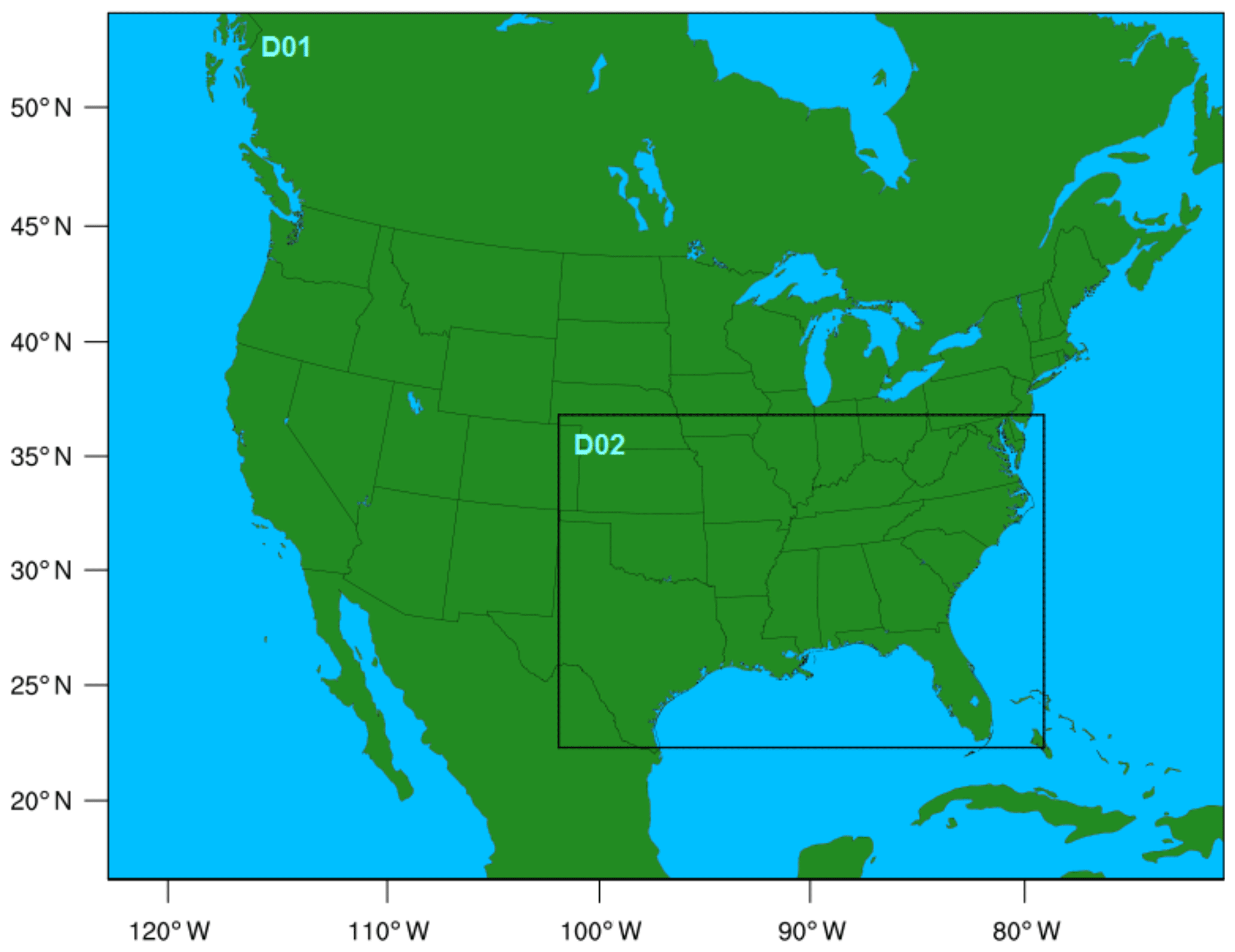
Figure 1Modeling domains for the meteorological model: D01 at 50 km × 50 km grid spacing and D02 at 12 km × 12 km grid spacing.
Meteorological inputs for the dynamical d-s AAB estimates were provided by the Weather Research and Forecasting model (WRF – Skamarock et al., 2008) over domain D02. This involved the use of WRFG (WRF with an improved scheme for convective parameters – Grell and Devenyi, 2002) model outputs archived in the North American Climate Change Assessment Program (NARCCAP – Mearns et al., 2009) database for the D01 domain (Fig. 1) at 50 km × 50 km spatial resolution from the dynamic downscaling of a CGCM version 3.0 (Flato, 2005; Jeong et al., 2012) realization, with the same A2 scenario for GHG emissions as in the previous case. These D01 WRFG outputs were used at the boundaries of domain D02 for a WRF version 3.4.1 simulation using its nest-down feature at 12 km × 12 km resolution to calculate the meteorological inputs needed for the AAB estimates. The model differences between WRFG and WRF version 3.4.1 and their implications for the dynamical d-s wildfire emissions inventory are discussed in Shankar et al. (2018).
Each set of AAB estimated as described in Prestemon et al. (2016) and (Shankar et al., 2018) was used to calculate daily wildfire emissions with the BlueSky/CONSUME fire consumptions and emissions model (Larkin et al., 2009). A critical step in this process is the disaggregation of the AAB estimates into daily fire activity with a daily metric of ignition probability, the fire weather index (FWI – Stavros et al., 2014), using the Fire Scenario Builder (McKenzie et al., 2006). Due to the finer (daily) temporal resolution of the meteorological data needed to calculate the FWI than is available from statistical downscaling, the same WRF model outputs were used to disaggregate the AAB to daily area burned for both statistical d-s and dynamical d-s (Shankar et al., 2018).
As a baseline inventory, the 2010 NEI for wildfire emissions draws on a variety of data sources, including fire counts, i.e., fire pixels at 1 km2 resolution, from the Moderate Resolution Imaging Spectroradiometer (MODIS) on board the Aqua and Terra satellites, available in the National Oceanic and Atmospheric Administration's Hazard Mapping System. These are matched in the SMARTFIRE system (SMARTFIRE – Raffuse et al., 2009; Pouliot et al., 2012) to ground-based wildfire activity data reported in Incident Status Summary (denoted as ICS 209) reports by the National Interagency Fire Center. The daily areas burned estimated by SMARTFIRE are input to the Fire Emissions Processing System (FEPS) in BlueSky (Larkin et al., 2009) to estimate daily point wildfire emissions for the NEI (Pouliot et al., 2008). Being an empirical inventory, the NEI does not include changes in climate and socioeconomic variables and is intended for use in AQ simulations close to the time period of the inventory data.
Each of the three wildfire inventories was processed in the Sparse Matrix Operator Kernel Emissions (SMOKE) processing system (Houyoux et al., 2000; Baek and Seppanen, 2018) to provide the necessary spatiotemporal wildfire emission magnitudes for the respective AQ simulation, which were then vertically allocated inline by the AQ model. The diurnal profiles and fire emissions speciation for PM used in the NEI benchmark inventory were also applied in processing the other two inventories, to avoid any artifacts from them in the inventory comparisons. Emissions for all other source sectors were provided by the EPA's 2005 NEI for all three cases. Table 1 summarizes these details.
Table 1Summary of cases simulated in modeling study.
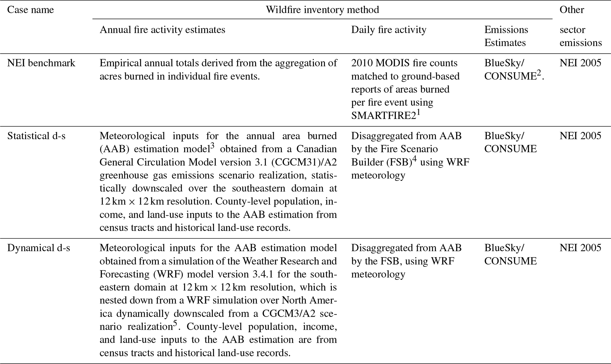
N.B: With the exception of the wildfire emissions, all CMAQ simulations were performed for the southeastern domain (denoted D02 in Fig. 1) at 12 km × 12 km grid spacing using identical meteorological, boundary, and other inputs and model configurations. 1 Pouliot et al. (2008). 2 Larkin et al. (2009). 3 Prestemon et al. (2016). 4 McKenzie et al. (2006). 5 Mearns et al. (2009).
2.2 Air quality simulations
The CMAQ v5.0.2 model simulations for the 2010 evaluation study were performed over the southeastern US domain shown in Fig. 1 (D02) at a 12 km × 12 km horizontal grid spacing. Representative hourly chemical boundary inputs at the lateral boundaries of the domain were extracted from an annual simulation for the conterminous US (CONUS) at 36 km × 36 km grid spacing (Vennam et al., 2014) for all three simulations. All simulations also used the same aerosol- and gas-phase chemical mechanisms. The carbon bond 05 gas-phase mechanism (cb05tucl) used in our simulations includes updates to toluene chemistry, homogeneous hydrolysis rate constants for N2O5, and updates to the chlorine chemistry (Sarwar et al., 2011; Whitten et al., 2010). The aerosol mechanism, AERO6, includes a primary organic aerosol aging scheme (Simon and Bhave, 2012) and an improved representation of fugitive dust; primary speciated emissions needed to model dust are based on Reff et al. (2009).
2.3 Observational networks
Observations for ozone and speciated PM2.5 for 2010 were extracted from three long-term monitoring networks: the Air Quality System (AQS – https://www.epa.gov/aqs, last access: 25 November 2019), a national network of over 1000 sites maintained by the EPA; the Interagency Monitoring of PROtected Visual Environments (IMPROVE – Sisler et al., 1993), a network of mostly rural sites concentrated in the western half of the US, and the EPA's Chemical Speciation Network (CSN – https://www3.epa.gov/ttnamti1/speciepg.html, last access: 25 November 2019) of mostly urban sites. AQS consolidates and distributes data on samples taken at hourly and daily intervals. The IMPROVE and CSN observations are for two 24 h periods per week, with many colocated sites so that they provide observations of rural vs. urban air sheds in close proximity. We also compared simulation results to available observations of hourly ozone and daily averaged speciated PM from the Southeast Aerosol Research and Characterization (SEARCH – Blanchard et al., 2013, and references therein) network for the continuous monitoring of particulate matter (PM) over a limited set of eight sites in the southeastern US.
2.4 Model evaluation tools and data
The Atmospheric Model Evaluation Tool (AMET – Appel et al., 2011) was used to compare the modeled cases against each other and against the network observations, using mean fractional error (MFE), mean fractional bias (MFB), normalized mean error (NME), and normalized mean bias (NMB) as the key indicators of model performance. In model-to-observation comparisons all four metrics are meaningful, but in intermodel comparisons AMET also calculates “bias” of one model with respect to another, which is useful for testing our hypothesis regarding the performance of our projection methods with respect to the NEI benchmark. The AMET version used here (version 1.2.2) contains several updates to the tool since the initial distribution, along with corrections to the observational data originally distributed with the software. In our intermodel comparisons, we filtered the model results to display only monitored grid cells that had wildfires, defined as those with nonzero AAB estimated for the statistical d-s case described in Shankar et al. (2018). This case was deemed to have the most number of grid cells with fires among the three inventories and to have AAB most similar to the gap-filled AAB data (Prestemon et al., 2016) created for the historical period 1992–2010. Most model grid cells in this dataset had some fires, and therefore our analyses apply to most of the domain.
3.1 Ozone
3.1.1 Model evaluation against observations
In this section, we compare the performance of the two downscaling methods to observations for ozone. We also provide results using the NEI benchmark wildfire inventory for reference. We evaluate the ozone model performance against AQS observations over all of 2010. Boylan and Russell (2006) provide the performance guidelines in current use in AQ model evaluation for MFB and MFE, with respect to observations for ozone and PM, that are considered good, acceptable, or needing further investigation. We also apply the recently recommended ozone performance metrics of Emery et al. (2017) for monthly averaged NME, NMB, and correlation coefficient r, shown in Table 2 along with mean modeled and observed ozone. We compare the region-wide MFB and MFE for modeled monthly averaged 1 h ozone relative to AQS measurements in the soccer goal plots of Fig. S1 in the Supplement, with the performance goals and criteria of Boylan and Russell (2006) shown as dotted lines. The ozone performance statistics show very small differences in the CMAQ results from the three sets of wildfire emissions. Table 2 shows that in all three modeled cases, ozone is overestimated in all months of the fire season (March–November) and the ozone model performance falls outside the performance criterion of NME ≤25 % in all months, although it meets the criterion for NMB ( %) in December–April and October and for the correlation coefficient r (>0.5) in every month. Although Table 2 shows that the observed monthly averaged ozone was below the recommended 40 ppb cutoff for applying these criteria in all months, we consider all of them because of the sporadic nature of wildfire and its impacts on air quality, especially since these are monthly averaged mixing ratios. MFB and MFE in Fig. S1 are in the acceptable range of performance for ozone (≤50 % and %, respectively) from March to July but fall just outside of it from August to November. The overprediction is greatest in the summer, especially August, being 8.4 ppb for the statistical d-s, while the best agreement with observations within the fire season is for April in all three cases (Table 2). However, differences among the three cases are negligible. Of the three cases, the statistical d-s case has the largest MFB, albeit by a very small margin, in October. There is virtually no disagreement between the dynamical d-s and NEI benchmark cases throughout the fire season except in September. It is important to note that there are no wildfires in January, February, and December in any of the inventories, and thus the emissions for these months are the same across all three modeled cases, corresponding to the NEI 2005 (default) inventory.
Table 2Model performance statistics for monthly averaged ozone vs. AQSa observations.
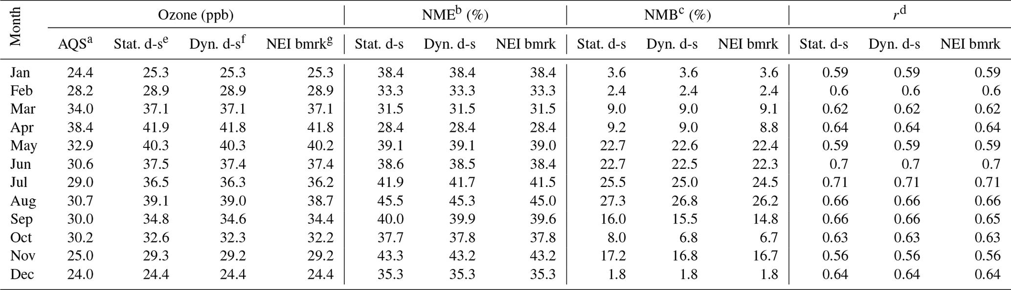
a AQS: air quality system. b Normalized mean error. c Normalized mean bias. d Correlation coefficient. e Statistical d-s. f Dynamical d-s. g NEI benchmark.
Based on the statistics in Table 2 and Fig. S1 there are no discernible differences in their monthly average performance over all sites and hours in any month, with a small exception in October for the statistical d-s. This is confirmed by the lack of distinction among the cases in the seasonal spatial distributions of MFB (Fig. S2 in the Supplement), with the exception of one AQS site on the Kentucky–Illinois border in autumn. The MFB has some of its largest values in the eastern half of the domain in spring and is lowest in autumn domain-wide. Comparing hourly ozone across networks in Fig. S2, the SEARCH network sites (four rural, four urban) in the Deep South show lower biases than the AQS sites across the three cases and seasons. The lack of distinction across the modeled cases for either network is consistent with the results for the absolute difference in hourly ozone between the two downscaling methods in the 24 h domain-wide trend (Fig. S3 in the Supplement), thus, at most hours of a given day over the whole domain, 75 % of the values modeled by these two methods differ by ∼0.1 ppb or less.
To better understand the relative contributions of the magnitude and location of the wildfire emissions to the October 1 h ozone performance differences among our three methods, we filtered the three sets of modeled data over the range of values showing the largest differences, at all grid cells that contained monitors and also had some fire during the fire season. We then examined the hourly O3 for October at a few of these selected locations (Fig. S4 in the Supplement). Figure S4a–d show the time series of ozone mixing ratios and bias with respect to observations for all three modeled cases at two AQS sites, 2105900005 and 210910012, close to the Kentucky (KY) and Ohio (OH) border labeled KY–OH (1) and KY–OH (2), respectively. Figure S4e–h display the time series for the same metrics at AQS sites 291831002 and 295100085 farther west, on the Missouri (MO) and Illinois (IL) border (labeled MO–IL (1) and MO–IL (2), respectively). These four sites had some of the largest differences in the statistical d-s case relative to the other two cases in the low-to-middle range of values (0–70 ppb) during the fire season (see Table 3). With the exception of short periods of large positive differences in the statistical d-s case from the other two cases on specific days in October, they are all closely aligned; some smaller differences are also seen between the dynamical d-s and the NEI benchmark. At the KY–OH sites, all model simulations underpredict the ozone peaks during 9–11 October with the NEI having the greatest underprediction, while all models have an equally high bias during 24–26 October. The statistical d-s case shows a large overprediction on 30 October. The similarity of the temporal trends at these two proximal sites suggests similar sources of the biases. The two sites at the MO–IL border show less negative bias in the models relative to AQS observations, but once again the statistical d-s has large positive biases with respect to the other cases and to AQS for short periods mid-month and at the end of the month. Its negative biases with respect to observations also tend not to be as large as in the other two cases, e.g., on 11 October at the KY–OH (1) site. This would be expected, as this case had the largest AAB values of the three inventories (Shankar et al., 2018).
Table 3Ozone at selected locations from statistical d-s, dynamical d-s, and AQSa network observations.
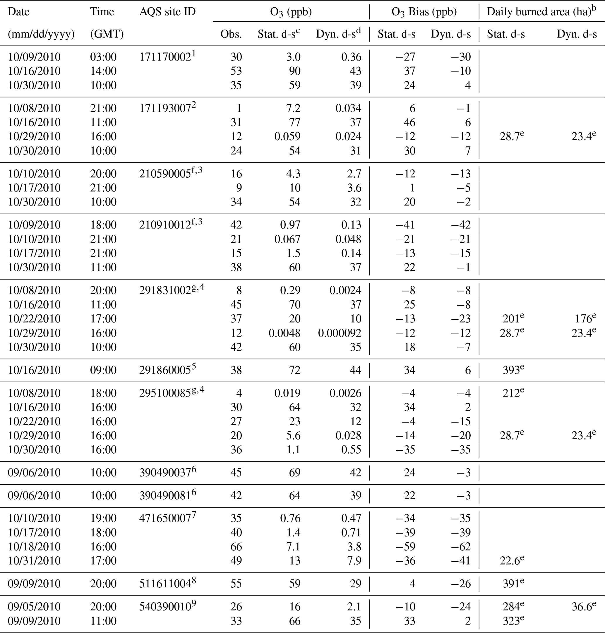
a Air Quality System.b A blank in these columns indicates that there were no areas burned inside or within a few grid cells of the monitored cell. c Statistical d-s. d Dynamical d-s. e Denotes the area burned in an upwind location within 1–2 grid cells of the monitored cell. f KY–OH sites in Fig. S4. g MO–IL sites in Fig. S4. AQS site key: 1 Nilwood, Illinois; 2 Wood River, Illinois; 3 Owensboro, Kentucky; 4 St. Louis, Missouri; 5 Bonne Terre, Missouri; 6 Columbus, Ohio; 7 Hendersonville, Tennessee; 8 Roanoke, Virginia; 9 Charleston, West Virginia.
Results of our time series analyses at these and other AQS sites are tabulated in Table 3, highlighting periods and locations of large differences either between the two downscaled cases, or between one or the other case and AQS observations. Most of these occurred in October 2010, but there were also a few outlier locations and times in early September. Ozone is underpredicted at half the locations and times in the statistical d-s case and at 76 % of them in the dynamical d-s. The model biases with respect to AQS vary between −49 and +47 ppb for statistical d-s and between −62 and +13 ppb for dynamical d-s. The largest intermodel differences occur in grid cells on days with little or no fire activity within or near the cells; most of the grid cells indicated as no-fire locations in Table 3 had fewer than 5 ha burned annually. Thus, the biases are not proportional to daily fire activity within the grid cell, but, in general, when there is a large difference in ozone between the two modeled cases, there is a comparable difference between them in daily area burned in an adjacent cell upwind, which is larger for the statistical d-s due to its larger AAB as noted previously. There are also some dates, e.g., 30 October, on which the model biases with respect to observations are comparably large at multiple monitor locations, suggesting the impact of the same upwind fire event(s) at these locations. We explore this further in the next section.
3.1.2 Intermodel comparisons
Hourly ozone
The modeling bias with respect to AQS observations is shown in the previous analyses to be very comparable among the three wildfire emission estimation methods; this may mask intermodel differences and prevent understanding of important sources of modeling uncertainties. Therefore, we compare the differences in modeled 1 h O3 mixing ratios between each pair of the three CMAQ simulations at AQS sites for the whole fire season (1 March–30 November) and for the months with the maximum differences (Fig. 2). For the whole wildfire season, the statistical d-s ozone values are the highest and the NEI values are the lowest. The maximum difference with respect to the NEI exceeds 45 ppb for both downscaling methods (Fig. 2a, b, d, and e). Of these, statistical d-s has the largest maximum difference compared to the other cases (>67 ppb) and systematically positive domain-wide mean differences (denoted MB in the figure) compared to dynamical d-s and NEI of 0.12 and 0.23 ppb, respectively, over the fire season (Fig. 2a and c). Comparable maximum differences of >67 ppb between the statistical d-s and either of the other cases occur on 29 October (Fig. 2d and f) due to an outlier value in the statistical d-s predictions at AQS station 291893001 and nearly identical low ozone values there in the dynamical d-s and the NEI cases for that hour. The maximum difference between the dynamical d-s and the NEI of 45.7 ppb occurs on 6 July at a different station (540390010), and, even with a positive mean difference with respect to the NEI of 0.1 ppb over the fire season (0.17 ppb in July), most of the dynamical d-s values are within 50 % of the NEI (Fig. 2b and e).
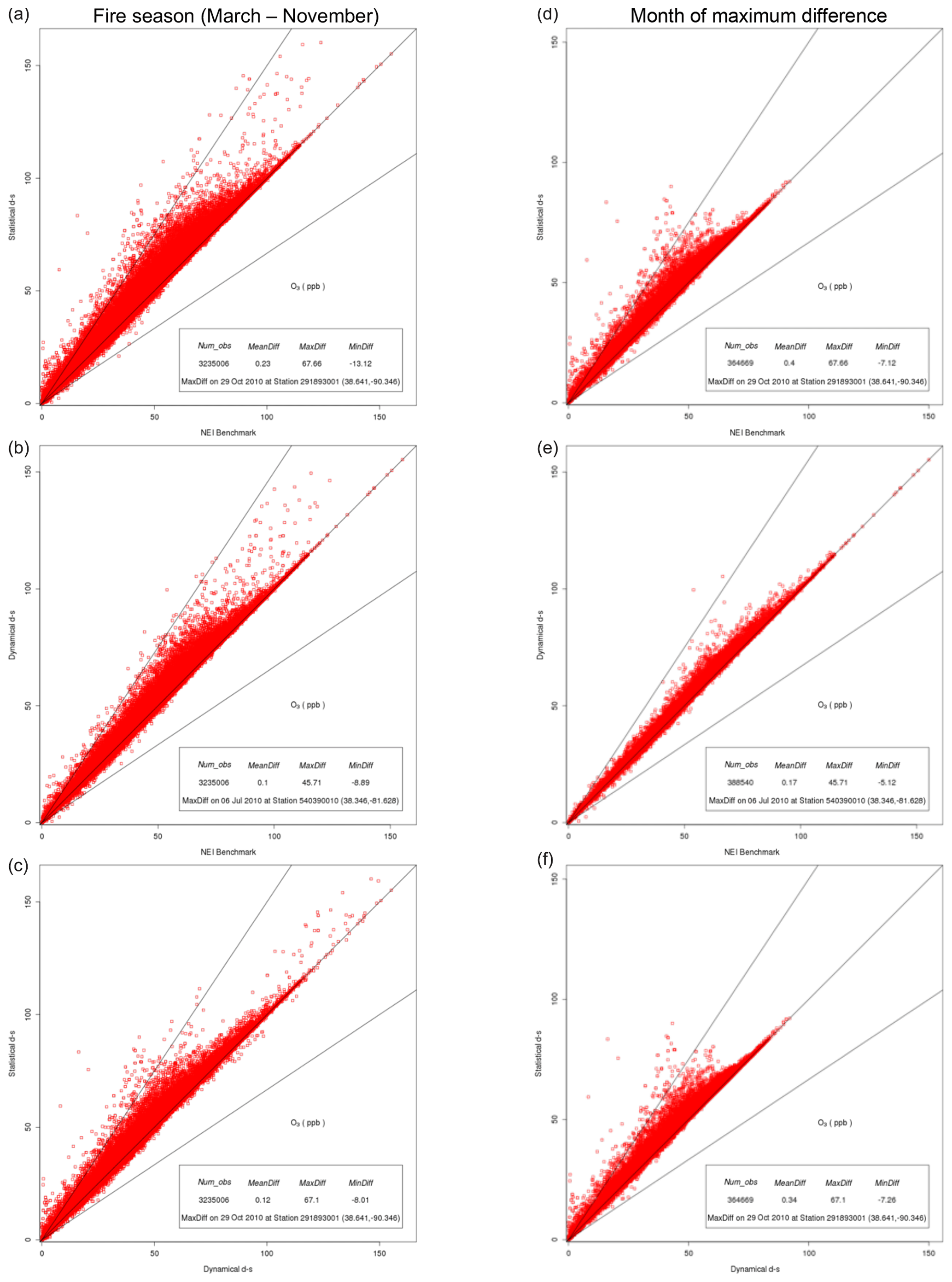
Figure 2Comparisons of each pair of wildfire emissions methods for 1 h O3 (ppb) predicted at grid cells containing Air Quality System (AQS) monitors and wildfires in 2010. (a, d) Statistical d-s vs. NEI benchmark, (b, e) dynamical d-s vs. NEI benchmark, and (c, f) statistical d-s vs. dynamical d-s. Monthly simulations are for (d, f) October and (e) July.
To better distinguish between outlier values and more systematic biases in ozone, we compared the three cases in each season (Fig. 3). Seasonally, the springtime differences are the smallest between each pair of cases compared, as would be expected due to low fire activity. Summer ozone differences between each pair of cases (Fig. 3b, e, and h) have a smaller range and lower values (0.12–0.28 ppb) than in autumn (0.11–0.32 ppb; Fig. 3c, f, and i). Comparing across modeled cases, the systematic positive mean ozone differences in either downscaling method compared to the NEI persist in each season (Fig. 3, a, b, d, e, g, and h). The largest seasonal mean difference from NEI is in autumn in the case of statistical d-s (0.32 ppb) and in summer in the case of dynamical d-s (0.15 ppb); the latter difference is likely due to a few outlier locations, as autumn actually shows a greater range of differences from NEI for this case. Over all seasons, there is better agreement between the dynamical d-s and NEI than between the statistical d-s and NEI. The reasons underlying these intermodel biases are explored in Sect. 3.1.3 (Discussion). The previously noted positive mean difference in the statistical d-s results relative to the dynamical d-s increases progressively from 0.05 to 0.21 ppb from spring to autumn (Fig. 3g–i).

Figure 3Seasonal comparisons of each pair of wildfire emissions methods for 1 h O3 (ppb) predicted at grid cells containing both Air Quality System (AQS) monitors and wildfires in 2010. (a, b, c) Statistical d-s vs. NEI benchmark, (d, e, f) dynamical d-s vs. NEI benchmark, and (g, h, i) statistical d-s vs. dynamical d-s.
Daily maximum 8 h average ozone
Although hourly ozone performance is a good indicator of the robustness of the gas-phase chemical mechanism in the model, in regulatory compliance modeling in the US, the maximum value of the 8 h running average of ozone mixing ratio over a given day (denoted MDA8) is the metric of relevance. Its calculation is a requirement for state-level demonstrations of attainment of the annual ozone standard (U.S. EPA, 2007). Our comparisons of MDA8 between each pair of CMAQ simulations (Figs. S5 and S6 in the Supplement) show similar characteristics to those for 1 h ozone. Overall, most of the MDA8 values show better agreement between the cases than the 1 h values (within ±50 % of each other), as might be expected from the longer averaging periods for this metric. However, as for 1 h ozone, the mostly positive differences remain for either downscaling case with respect to NEI and for the statistical d-s with respect to the dynamical d-s case. There is also more variability in the timing and location of these maximum intermodel differences (Fig. S5d–f). They occur on 6 July for the statistical d-s case vs. NEI (33.4 ppb), on 3 September for the dynamical d-s case vs. NEI (30.2 ppb), and on 16 October for the statistical d-s case vs. the dynamical d-s case (28.3 ppb). Seasonally (Fig. S6), both downscaling cases have large differences from the NEI at the upper end of the range in autumn, an indication of their higher wildfire emissions estimates than in the NEI in this season.
Ozone modeling uncertainties
Table 2 and Fig. S4 illustrate the large differences among the downscaled inventories in relatively fire-free locations, possibly due to a greater impact in these environments from the transport of precursors and ozone from fires upwind. This is supported by the spatial distribution of the maximum absolute difference in O3 and its precursor emissions between statistical d-s and dynamical d-s in each modeled grid cell over the entire fire season (Fig. 4). In this comparison “fire season” is defined as 23 April–30 November 2010 because that was the period of occurrence of these maximum differences. The spatial pattern for O3 (Fig. 4c) shows that the geographic areas of greatest difference in O3 are in the Appalachian region centered in West Virginia and also in “plumes” into the southwestern corner of Missouri and out of its eastern border. The spatial pattern of these differences appears to be aligned with an underlying circulation, suggestive of transport from upwind source regions. This possibility is borne out by the spatial patterns of the maximum absolute difference in the column totals of volatile organic compounds (VOCs) and NOx point emissions between the two respective wildfire inventories (Fig. 4a and b) over the same period. Column emission totals, rather than emissions in model layer 1, are used in this comparison because they constitute the wildfire emissions from each inventory, including what is allocated to aloft layers and transported downwind in the AQ simulation and which would be missed if the comparison had been limited to emissions in layer 1. The largest differences are seen in VOC emissions due to their much greater magnitude than those of NOx, but both precursors have similar spatial patterns of maximum absolute difference between the inventories. Peak differences occur in both species emissions from the southwestern corner of Missouri and across its lower third, as well as at the KY–OH border in Appalachia, south and east of the ozone difference peak in West Virginia seen in Fig. 4c.
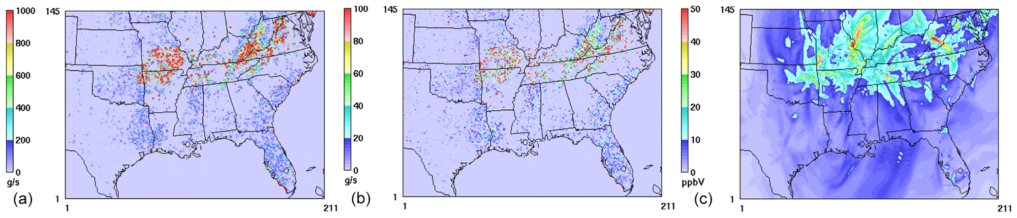
Figure 4Maximum absolute difference between statistical d-s and dynamical d-s in each grid cell over the whole fire season in (a) hourly VOC column emissions (g s−1), (b) hourly NOx column emissions (g s−1), and (c) hourly O3 mixing ratios (ppbV) in model layer 1. Here the fire season is defined as 23 April–30 November; almost all grid cell maxima in absolute hourly O3 difference occurred in this time period.
3.1.3 Discussion
Overall, our analyses of ozone model performance over the fire season show very little difference among the three modeled cases with respect to each other but a consistent and near-identical overprediction of ozone across all three, with the largest MFE (55 %) occurring in the winter. The sharp differences seen in our results at individual locations and times in the intermodel comparisons (Figs. 2, 3, S5, and S6) between the two downscaled cases do not translate into major differences in the overall 1 h and MDA8 ozone model performance, with the possible exception of statistical d-s in October. In all cases the largest MFEs occur in winter, outside the fire season (Fig. S1). As the three inventories used in the simulations differ only in the wildfire emissions, the occurrence of the maximum MFE in winter indicates that those emissions are not the major contributor to the ozone biases for any of the cases. This is consistent with the findings of Wilkins et al. (2018), whose brute-force zero-out analyses of wildfire emissions impacts on air quality showed only a 1 % increase in ozone due to wildfire from 2008 to 2012 over the CONUS.
Despite the very slight differences in error statistics among the three modeled cases for hourly ozone during the fire season, our intermodel comparisons do show sporadic large differences between the statistical d-s and the other two cases and somewhat smaller ones between the dynamical d-s and the NEI. Differences in model formulations used in the two meteorological downscaling methods, which can lead to spatiotemporal differences in their predictions of peaks and troughs in wildfire emissions, are discussed in Shankar et al. (2018). The biases between the two downscaling methods are due to fundamentally different formulations of the underlying models used to provide the climate inputs for the AAB estimation. Statistical downscaling is a closer representation of the large-scale circulations modeled by the GCM used in the climate downscaling, while the dynamical d-s captures more of the prevailing local meteorological features, which may be quite different in a given period from the large-scale circulation. Furthermore, the WRF 3.4.1 model used in the AAB estimates for the dynamical d-s inventory has a known high precipitation bias (Alapaty et al., 2012; Spero et al., 2014). The prediction of too much precipitation in the AAB estimation model inputs could be another reason for the lower wildfire emissions overall in the dynamical d-s case (Shankar et al., 2018); this would account for its lower ozone precursor emissions and mixing ratios compared to the statistical d-s case. Temporally, some of the largest differences in 1 h ozone between the two downscaling cases occur on the same day, e.g., 30 October, at multiple locations. Spatially, they occur in relatively clean, i.e., low- or no-fire grid cells. These results suggest that the greatest impact of their different wildfire emissions magnitudes is on ozone mixing ratios in low- or no-fire grid cells due to the transport of those emissions (and ozone) from upwind locations with significant fire activity.
The seasonal intermodel comparisons of Fig. 3a–f show that the two downscaling methods differ not only in the magnitude but also the timing of the maximum difference with respect to the NEI. The NEI predicts less ozone than the other cases in all the warmer months (summer and autumn). These warmer months are dominated by fires in a denser canopy. MODIS fire counts, which are used to estimate area burned in the NEI, are known to be underestimated in the earliest versions of that inventory for wildfires, in part due to the difficulty of under-canopy detection of small fires by the MODIS instrument (Pouliot et al., 2008; Soja et al., 2009). In addition to any ozone overestimates that are present in the downscaling cases in these months (e.g., statistical d-s in October), application of the MODIS estimates during canopy-heavy months could also contribute to these lower values in the NEI relative to the downscaling cases. The seasonal (positive) differences in ozone among the models are largest between either downscaling case and the NEI in autumn at the upper end of the range and can be attributed to the effect of less convective precipitation in autumn than in summer in the southeastern US, which would increase the daily fire activity estimates in the downscaling cases.
3.2 PM2.5
3.2.1 Model evaluation against observations
In this section, we compare the performance of the two downscaling methods and the NEI wildfire inventory to PM2.5 observations. We evaluate PM2.5 model performance over all of the 2010 fire season (1 March–30 November), as well as its seasonal variability, using observations from the IMPROVE, CSN, and the SEARCH networks for PM2.5 and its constituents.
Monthly variability
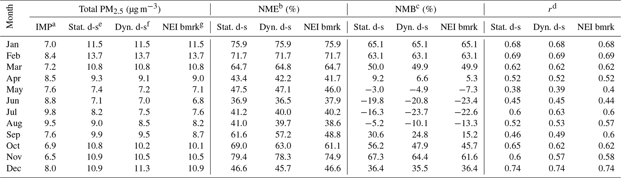
Table 4 summarizes the performance statistics (NME and NMB) for PM2.5 compared to observations from the IMPROVE network. There is more variability in these metrics seasonally and among the three simulation cases than in the results for ozone (Table 2). Figure 5 shows the range of MFE and MFB for total PM2.5 and for two key co-emitted PM constituents from wildfires, elemental carbon (EC), and organic carbon (OC). The overall performance for PM2.5 (Fig. 5a–c) is in the acceptable range for MFE and MFB (≤75 % and %, respectively) in all months. It meets the stricter criteria of Emery et al. (2017) for NME and NMB (<50 % and %, respectively) in April–September (Table 4). Unlike ozone, which is overpredicted in the summer months, total PM2.5 has the greatest underprediction in these months in all three cases, with the statistical d-s having the least negative bias with respect to observations, followed by the dynamical d-s (except in July). The best performance statistics are in April and May, while the greatest overpredictions during the fire season are in November and March. However, these last 2 months appear to be in a continuum of overpredictions from late autumn when they are largest to early spring when they are smallest across all cases. The NEI has the best performance of the three cases for total PM2.5 in the spring and autumn months and the most underprediction in the summer months, though by small margins.
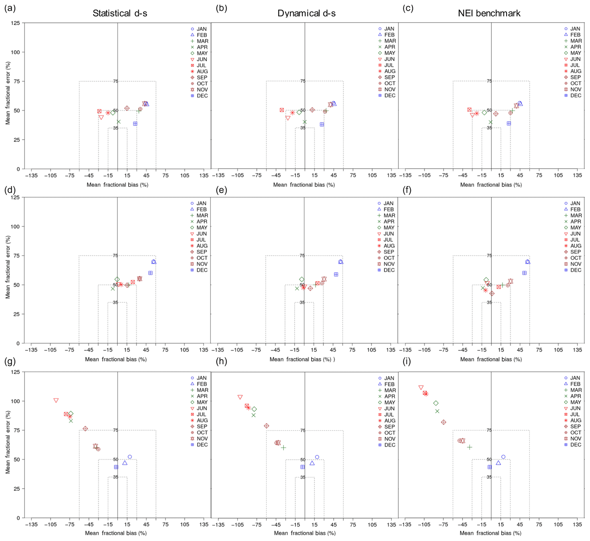
Figure 5Monthly averaged model performance for total PM2.5 and key wildfire constituents relative to observations from the IMPROVE monitoring network: (a, b, c) PM2.5, (d, e, f) elemental carbon (EC), and (g, h, i) organic carbon (OC).
Table 4Model performance statistics for monthly averaged total PM2.5 vs. IMPROVEa observations.
a Interagency Monitoring of PROtected Visual Environments
network. b Normalized mean error. c Normalized mean
bias. d Correlation coefficient. e Statistical d-s.
f Dynamical d-s. g NEI
benchmark.
To investigate the possible source(s) of the PM2.5 biases, we examined these error metrics for all the major PM constituents. The results for EC and OC are shown in Fig. 5d–f and g–i, respectively, and for the inorganic constituents (SO4, NH4, and NO3) in Fig. S7 in the Supplement. EC performance for all three cases meets the PM performance goal (MFE ≤ 50 % and MFB ≤ ±30 %) of Boylan and Russell (2006) in April, June, August, and September and meets their performance criteria (MFE ≤ 75 % and MFB ≤ ±60 %) in the remainder of the year. MFB for EC is nearly zero for the two downscaled cases and slightly negative for the NEI in June and August but is positive in July for all three cases. These results indicate that the pronounced negative bias in PM2.5 in the summer months over all cases is not attributable to EC. All three cases overpredict EC in autumn, albeit within the good-to-acceptable range of performance. As there are no fires in the winter months, the performance for EC during that period is identical in all cases, and the large positive winter bias in EC is clearly due to combustion sources other than wildfires.
There is a severe underprediction in OC for all three cases, except in winter (Fig. 5g–i), with MFB from April to September being outside the range of acceptable performance. The negative biases are smallest for the statistical d-s, followed by the dynamical d-s, and largest for the NEI, particularly in summer and autumn, consistent with the progressive decrease in their respective wildfire PM2.5 emission magnitudes (Shankar et al., 2018) in these seasons. The negative biases in PM2.5 in the summer months, which are common to all three cases, are attributable in part to the OC underpredictions, although species with larger mass fractions of total PM could also be responsible. This is further examined in Fig. 6. OC performance is best in the winter months when there are no differences in the input emissions among the three cases; the performance also improves throughout the fire season from the warmest to the coolest months in all cases. We discuss some possible explanations for this in Sect. 3.2.3.
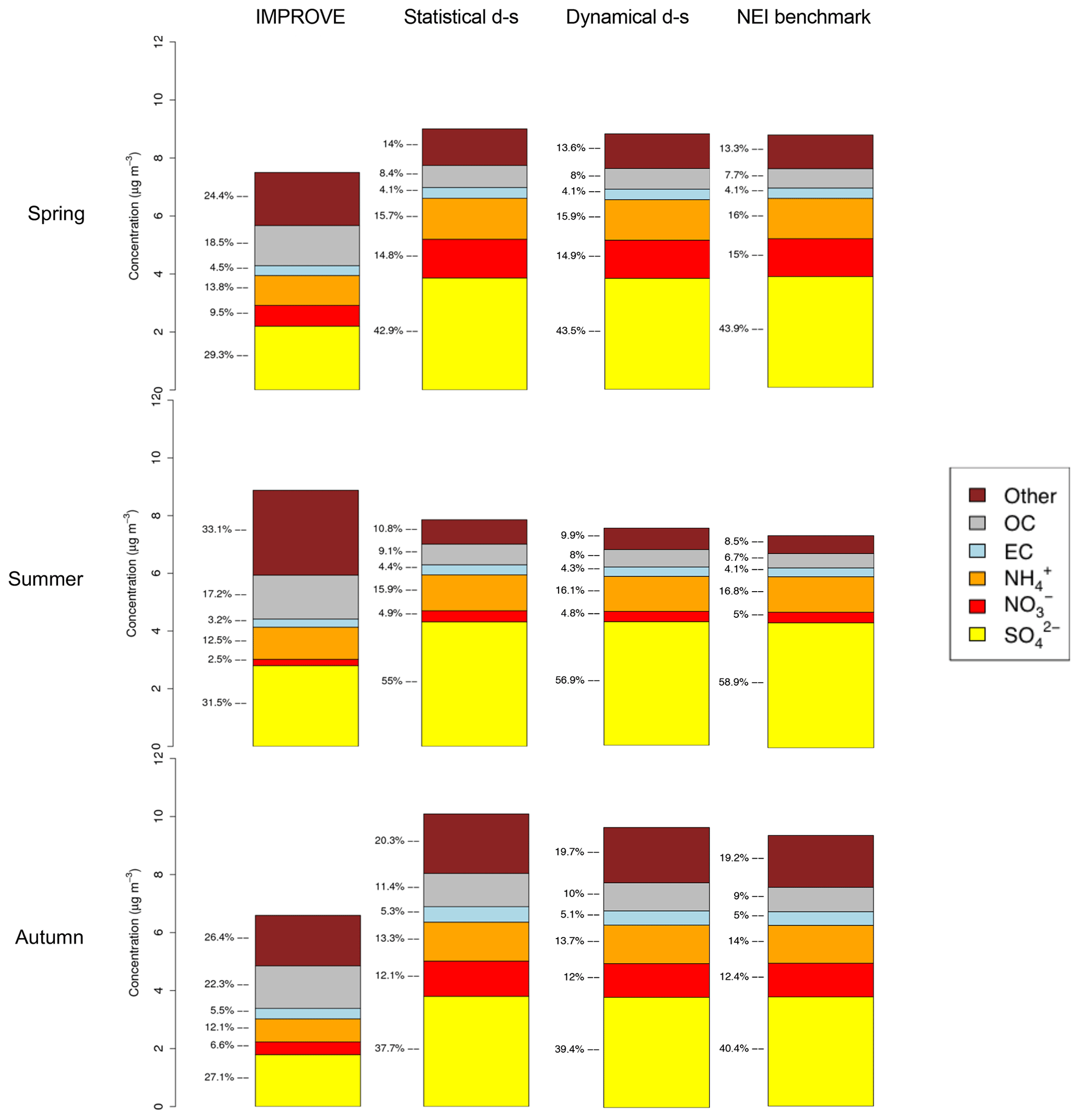
Figure 6Domain-wide seasonally averaged total mass of PM2.5 (µg m−3) and fractional mass of major constituents during the fire season compared to observations from the IMPROVE network.
Variability across network observations
The IMPROVE network is located mainly in the Federal Class I Areas with monitoring provided by the National Park Service (NPS) and administered by a consortium of several resource management agencies, such as the National Fish and Wildlife Service, the USDA Forest Service, the Bureau of Land Management. As such, IMPROVE monitors are placed in rural areas, which allow reliable measurements of ambient concentrations in the vicinity of fires. To evaluate the performance of our wildfire inventories in simulating air quality downwind and farther away from fires, we compared the model results at IMPROVE sites with those across the CSN and SEARCH networks for the species common to all. There are some limitations in these observations: the geographical coverage in SEARCH is limited to eight stations, located in Mississippi, Alabama, Florida, and Georgia, and CSN had no EC measurements available beyond March in 2010. Nevertheless, these cross-network comparisons can provide additional insights into the geographical variability of model performance for PM, e.g., urban vs. rural or the Atlantic seaboard vs. the high fire areas in the interior of the domain.
Total PM2.5 comparisons among IMPROVE and CSN (Fig. S8 in the Supplement) show that the model performance at the CSN sites is better than at IMPROVE sites, with lower bias and error, especially in the summer and autumn, for all three cases. In these warmer months, the least negative bias at the CSN sites is for statistical d-s in August and the least positive bias is for the NEI in September, but the differences among the cases are very small. Figure S9 in the Supplement compares the spatial distribution of MFB among the three modeled cases across available networks for total PM2.5 (IMPROVE and CSN) in each season. As with the ozone spatial comparisons of MFB (Fig. S1), the differences among the cases in Fig. S9 are too slight to be resolved in the color map. However, the bias differences across networks for PM2.5 in Fig. S8 indicate better performance in some of the constituent species in the warmer months at the urban sites than at the rural sites.
To investigate this further we compared monthly averaged model bias and error against IMPROVE, CSN, and SEARCH daily measurements (Fig. S10 in the Supplement) for OC and NO3. These are the two PM constituents with poor model performance at the IMPROVE sites (Figs. 5 and S7). As differences in model performance among the modeled cases were small in those comparisons, the Fig. S10 comparisons are shown for a single case, statistical d-s, which had large negative biases for OC and NO3 but also predicts higher PM2.5 than the other cases. The errors and biases for OC are comparably high at the IMPROVE and SEARCH networks and considerably less at the (urban) CSN monitors than at IMPROVE (rural) sites; possible reasons for this urban–rural bias in OC are examined in Sect. 3.2.3 (Discussion). However, the monthly variability of the bias is seen at the SEARCH and CSN monitors as well and goes from negative to positive progressively from the warm to cool months, as at the IMPROVE sites.
NO3 performance falls outside the acceptable range at all network sites, in almost all months, with CSN being the exception in winter. The results for NO3 are somewhat better at the IMPROVE and CSN sites than at SEARCH sites, which have considerably more underprediction from May to September. The seasonal variability of the bias at all three networks is similar to that of OC, at least in these months. As with OC, the greatest negative bias in NO3 is at the SEARCH sites in summer, with MFE in excess of 150 %. One contribution to this large value is from the low concentrations of NO3 in the southeastern US and the small numbers involved in the error estimates. The NO3 bias is discussed further in Sect. 3.2.3.
PM composition
There is a wide range of bias and error among PM and its constituents in Figs. 5, S7, and S10, and in Tables 4 and S1–S3 in the Supplement. Total PM2.5 does meet the criteria for acceptable PM performance of Boylan and Russell (2006) throughout the year and across all cases for MFB and MFE and meets the performance criteria of Emery et al. (2017) for NME, NMB, and r (<50 %, %, and >0.4, respectively) in April–September. To further examine the contributions of individual PM species to total PM2.5 performance we compared the seasonally averaged PM2.5 composition (Fig. 6) over the fire season between IMPROVE observations and the model simulations. Overall, modeled PM composition is overpredicted in sulfate and nitrate, underpredicted in OC, and has mixed results for the other constituents. Total PM2.5 mass is overpredicted in the spring and autumn and underpredicted in the summer in all cases; the summer underprediction is driven by the underprediction of most species other than sulfate, particularly the severe underprediction of the lumped species labeled “other”, which includes fugitive dust. There is a decrease in predicted total PM2.5 mass across the three cases, statistical d-s, dynamical d-s, and the NEI and in the same direction as the decrease in their wildfire emissions. This translates into a monotonic decrease in the springtime average PM2.5 concentration of ∼1 % from statistical d-s to dynamical d-s to NEI. In the summer and autumn, there is a 5 % decrease from statistical d-s to dynamical d-s and a ∼2 %–3 % decrease from the dynamical d-s to the NEI. The differences of modeled PM from the observations are much larger, from a low of −20 % in the summer for the NEI to a high of 50 % for the statistical d-s in the autumn, as noted in here and previously.
The contribution of sulfate to total PM concentration over the southeastern US is substantial (26 %–32 %) in the IMPROVE observations throughout the year and is overpredicted in every season across the three cases, although Fig. S7a–c show it to be within the acceptable range in all months except October. The sulfate overprediction also persists in 2 months of the winter (January and February), when all three cases have identical emissions inputs (Table S3); the small difference in the dynamical d-s case from the other two cases for December is due to ∼10 % fewer matched model–observation pairs for this case in December. Statistical d-s, by a slim margin, has the largest SO4 overprediction over the whole year among the three cases, with an average NMB of 65.3 % and average NME of 78.2 % (Table S3), because of the larger magnitude of wildfire PM emissions from which its SO4 emissions contributions are estimated.
Due to the use of a common (NEI) speciation profile, both ammonia (NH3) and gas-phase NO3 from wildfires are allocated the same fractions of total PM2.5 emissions in all three wildfire inventories and across all seasons. Particulate NO3 contribution to total PM2.5 mass in the IMPROVE observations is between 2.5 % in the summer, ∼8 % on average in the spring and autumn (Fig. 6), and as much as ∼25 % in winter (not shown). It has a positive MFB of 14 %–51 % in the cooler months of the fire season over all three cases (Fig. S7g–i) but has an equally negative MFB in the warmer months; the monthly biases are more or less uniform across the three modeled cases. Once again, the statistical d-s case has the highest NMB (234 %) for NO3 among the three cases (Table S5) in October. There is very little difference in the positive biases in the remainder of the year across the cases. On the other hand, ammonium (NH4), a PM2.5 constituent that partitions between SO4 and NO3, contributes a greater fraction to total PM2.5 mass on average (12 %–17 %) than NO3 does throughout the year (Fig. 6). Its bias is considerably less than that of NO3 across the three cases and comparable to that of SO4.
3.2.2 Intermodel comparisons
Daily average PM2.5
Our PM2.5 model evaluation shows that although there is slightly more variability in the model simulation results for PM2.5 than in those for ozone, these differences are much smaller than their differences from observations. Our intermodel comparisons of PM2.5 are motivated by the need to better understand modeling uncertainties and compensating errors and how they affect overall model performance. PM2.5 concentrations summed over all constituent species are compared among the three cases over the whole fire season and inter-seasonally (Figs. 7 and 8) at grid cells that contained both IMPROVE monitoring sites and wildfires at the temporal frequency of the measurements. There is less statistical power in these results than in those for ozone due to fewer monitors in IMPROVE than in AQS in the eastern US, in addition to the lower temporal frequency of the measurements (daily averages measured twice a week). As with ozone, however, the largest differences in PM2.5 are in the statistical d-s case with respect to the other two cases (Fig. 7a, c, d, and f). As with ozone, the smallest differences between cases occur in the spring and the largest ones occur in autumn (Fig. 8g–i). However, the dates of maximum intermodel differences do not coincide with those for ozone in most seasons, suggesting a different source contribution to these differences than that for ozone. This is explored in the next section.
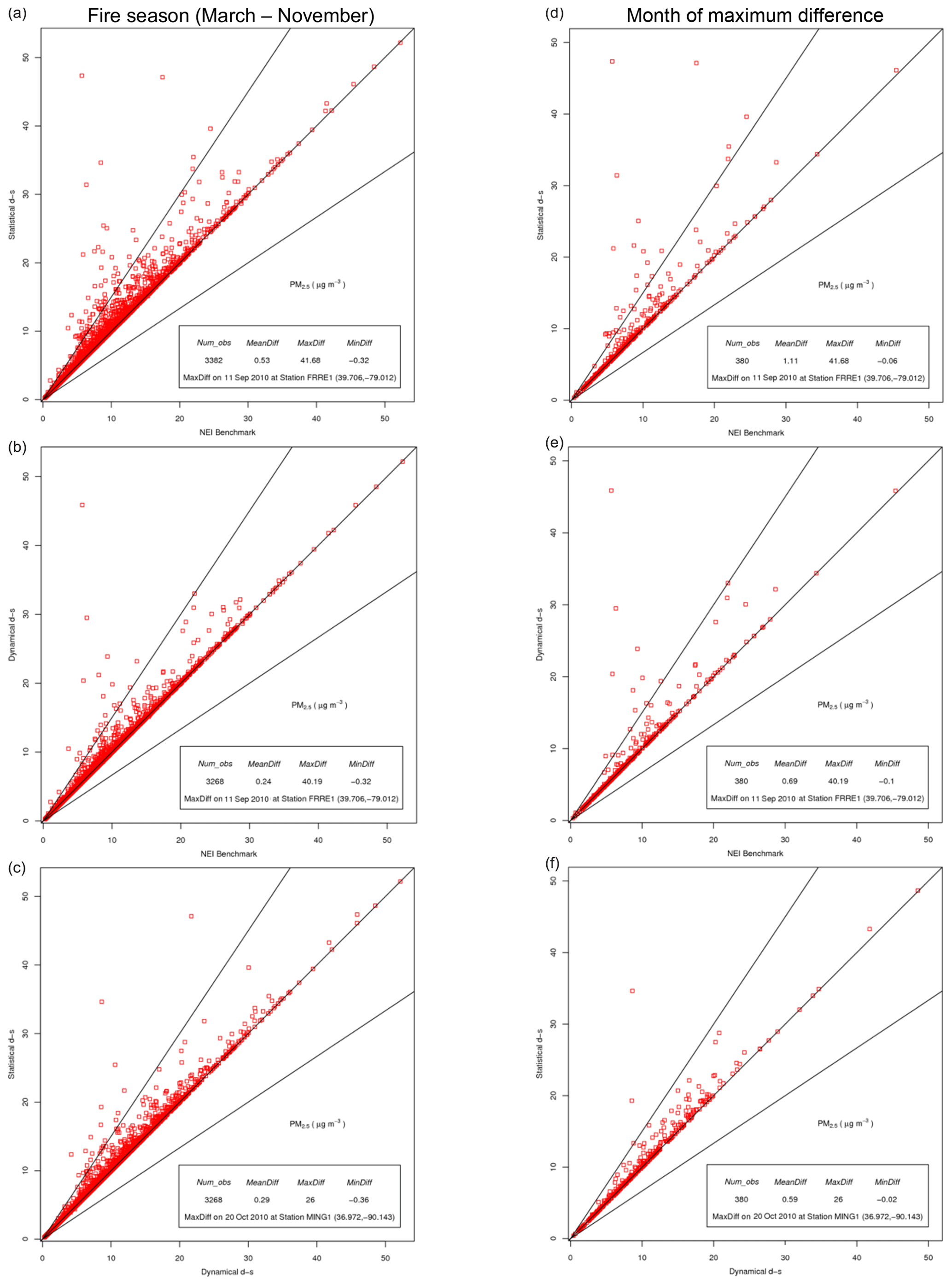
Figure 7Comparisons of each pair of wildfire emissions methods for PM2.5 (µg m−3) predicted at grid cells containing both Interagency Monitoring of PROtected Visual Environments (IMPROVE) monitors and wildfires in 2010: (a, d) statistical d-s vs. NEI benchmark, (b, e) dynamical d-s vs. NEI benchmark, and (c, f) statistical d-s vs. dynamical d-s. Monthly simulations are for (d, e) September and (f) October.

Figure 8Seasonal comparisons of each pair of wildfire emissions methods for PM2.5 (µg m−3) predicted at grid cells containing Interagency Monitoring of PROtected Visual Environments (IMPROVE) monitors and wildfires in 2010: (a, b, c) statistical d-s vs. NEI benchmark, (d, e, f) dynamical d-s vs. NEI benchmark, and (g, h, i) statistical d-s vs. dynamical d-s.
PM modeling uncertainties
The time frequency of PM2.5 measurements is twice per week in IMPROVE among about 28 sites in the southeastern US and thus considerably less than in the AQS measurements for hourly and MDA8 ozone. Nevertheless, for all the days available in the fire season at all the locations showing large differences (i.e., >50 %) between the downscaling cases, we performed a similar analysis to that for ozone. Table 5 summarizes modeled and observed results for PM2.5 at these outlier locations and their times of occurrence, which are somewhat different from those for ozone. The largest differences in PM2.5 occur in the summer, particularly in August. With the exception of James River Face in coastal Virginia, which is a few grid cells to the northeast of AQS site 511611004, there is little agreement in the locations of these large differences in PM2.5 with those in ozone and none in their dates of occurrence. This lack of agreement suggests a different underlying source of these occurrences for PM2.5 from that for ozone.
Table 5PM2.5 at selected locations from statistical d-s, dynamical d-s, and the IMPROVEa network.
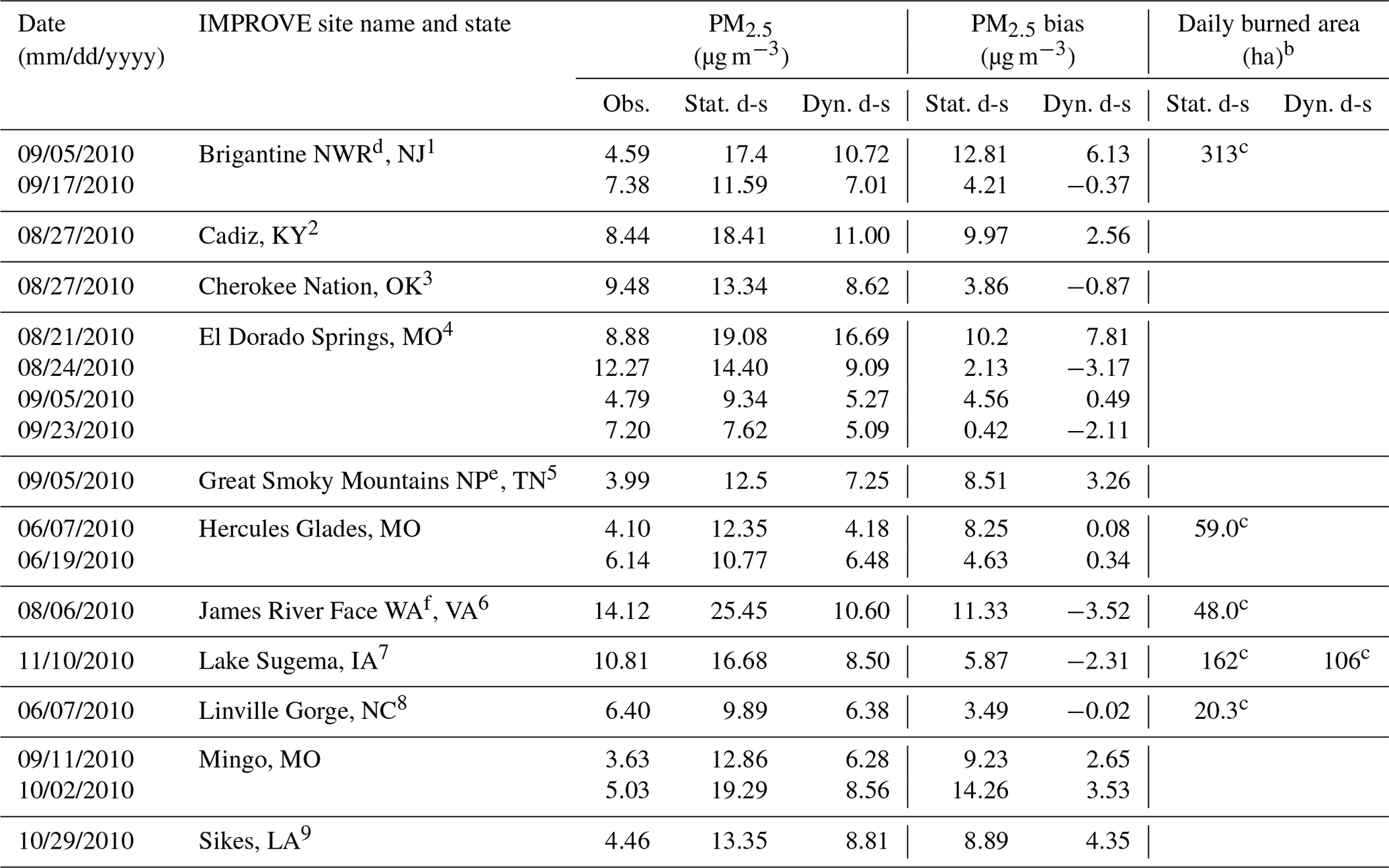
a Interagency Monitoring of PROtected Visual Environments network. b A blank in these columns indicates that there were no areas burned inside or within a few grid cells of the monitored cell. c Denotes the area burned in an upwind location within 1–2 grid cells of the monitored cell. Federal Class I Area designations: d national wildlife refuge, e national park, f wilderness area. State abbreviations: 1 New Jersey, 2 Kentucky, 3 Oklahoma, 4 Missouri, 5 Tennessee, 6 Virginia, 7 Iowa, 8 North Carolina, 9 Louisiana.
Despite the differences in the data of Tables 3 and 5, they do show some similarities. For all the 17 occurrences listed in Table 5 that show large differences in PM2.5 between the two downscaling cases, the statistical d-s case once again has the larger biases with respect to observations, ranging from 0.42 to 14.26 µg m−3. As with ozone, there is more negative bias (in 7 of the 17 occurrences) in the dynamical d-s case with respect to measurements, with the bias ranging from −3.52 to 7.81 µg m−3. Also, as with ozone, the difference in PM2.5 between the two cases in a given grid cell is not proportional to the differences in daily burned area within the cell, which is zero or negligible for both cases in most of the 17 occurrences. These large differences could be a result of the differences in daily fire activity in adjacent grid cells upwind, due to the larger burned area in the statistical d-s case than in the dynamical d-s case. This is true of each of the grid cells in Table 5 that had an adjacent grid cell with a fire on a given day.
As in the case of ozone, the domain-wide 24 h trend (Fig. S11 in the Supplement) of absolute difference in PM2.5 between the downscaling cases shows a very small median difference (on the order of 10−3 µg m−3) but with even less variability than for ozone and slightly more temporal variability at the upper end of the range than for ozone in Fig. S3. Primary emissions and their variability could contribute to a greater degree in these differences, as primary PM is a significant fraction (∼23 %) of these wildfire emissions excluding CO. The spatial distribution of the maximum absolute differences in PM2.5 throughout the fire season in the lowest model layer (right panel of Fig. S12 in the Supplement) shows a similar pattern overall to the ozone differences in that it is appreciable mostly over the central and northeastern parts of the domain. However, the spatial pattern for PM2.5 concentrations more closely resembles that of the column-total point wildfire emissions of PM2.5 (Fig. S12a), than in the case of ozone, particularly in southeastern Missouri and Appalachia. This indicates the greater role in the PM2.5 concentration differences played by primary wildfire PM emissions than in the case of ozone.
3.2.3 Discussion
Across all three cases modeled, PM2.5 shows an increasingly negative bias with respect to IMPROVE in the late spring through the summer, changing to a progressively more positive bias from autumn into winter, which has the largest MFE and MFB of 56.2 % and 44.5 %, respectively. The overall model performance for PM2.5 is acceptable in all cases but masks compensating errors in the PM constituents. Of these, the signature species for wildfires are EC and OC. Model performance for EC, which is primarily emitted in wildfires, is good-to-acceptable and mostly positively biased over the fire season. Taken alongside the poor performance for OC, which is mostly secondarily produced from precursors emitted from wildfires and other natural and anthropogenic sources, this indicates that wildfire EC emissions are not the driver of the pronounced negative biases seen in PM2.5 in the summer months. The OC biases are mostly negative and most pronounced in the warmer months; they are smallest for statistical d-s and greatest for the NEI, which, as noted previously, had an underestimation of emissions in the 2010 wildfire inventory due to the undercounting of fires below the canopy by MODIS (Pouliot et al., 2008). This underestimate would be greatest in the months when the canopy cover is greatest and could also account for EC being better predicted in June and August with the downscaled inventories than with the NEI inventory.
Another, and perhaps the biggest, contribution to the low bias in PM2.5 in summer comes from species other than the major organic and inorganic components (labeled “other” in Fig. 6). Other PM is an even larger fraction of the observed summer-average PM2.5 concentration than sulfate (Fig. 6). Fine PM is the second-largest component (∼ 43 %) after primary OC in wildfire PM emissions in all three inventories and is the primary contributor to other PM from wildfires in CMAQ. Given the uniform PM speciation profile across all seasons in all three wildfire inventories in this study and the relatively good comparisons of other PM with IMPROVE observations in spring and autumn, wildfire emissions are not the likely source of the poor summertime performance for this species. Fine dust episodes in the eastern US and the Caribbean in the summer have been shown through satellite observations to be associated with long-range transport from the Sahel (Prospero, 1999; Prospero et al., 2014). The severe summertime underprediction of other PM suggests a need to refine the eastern boundary conditions, which were the same across the three CMAQ simulations, specifically with respect to their intra-seasonal variability.
The large negative biases in OC predictions, which are seen across both rural and urban networks, are likely to be a result of underprediction in the CMAQ v5.0.2 secondary organic aerosol (SOA) mechanism rather than in the primary wildfire OC emissions. Some of the underestimation could come from the assumed NEI temporal profiles for emissions from smaller wildfires that are less than a full day in duration (Wilkins et al., 2018). Residential wood combustion has also been shown to be as a source of underestimation of carbonaceous PM in the NEI in a 2007 study over the southeastern US (Napelenok et al., 2014), and this possibility is supported by the better model performance for OC at CSN (urban) sites compared to IMPROVE (rural) sites. The potential role of residential wood combustion needs to be further examined within the context of the spatial and temporal distribution of emissions from this source for our modeling domain in 2010.
The very good performance for OC in the winter that gradually degrades going from cool to warm months is an indication that temperature dependence of precursor emissions may not be well represented either in the fire emissions model or in the SOA formation pathways in the CMAQ organic chemistry formulation. As the emission factors in the BlueSky fire emissions model do not adjust for the temperature dependence of individual PM species, the CMAQ SOA model is the most likely source of the seasonal variability of this bias. The underprediction of SOA in CMAQ is addressed somewhat by the volatility basis set (VBS – Donahue et al., 2013) implemented in a later version of CMAQ (CMAQ-VBS – Koo et al., 2014) than the one used here. However, large uncertainties still remain in the representation of semi-volatile and intermediate VOCs (IVOCs), especially in the primary emission estimates and in the SOA formation pathways, according to Woody et al. (2016). These authors have argued for improving the CMAQ-VBS model further by including representations of semi-volatile organic compounds (SVOCs) in the form of primary organic aerosol (POA) and IVOCs.
In contrast to OC, EC has its highest MFB and MFE in winter for all the cases modeled. As EC is co-emitted with OC in biomass and biofuel combustion, this indicates that the emission factors, and, in particular, the OC∕EC emission ratios used for non-wildfire combustion sources that are active in winter, e.g., biofuel, could account for the poor EC model performance. The monthly results for the EC and OC error metrics, which show a consistently higher MFB for EC than for OC indicate that the OC∕EC emission ratios could also be an issue in wildfire emissions.
Our PM composition analyses show that the constituent driving total PM2.5 performance is sulfate, due to its having the highest PM mass fraction. Wildfire emissions do not have a major source contribution to the modeled sulfate concentration. Primary SOx emissions constitute 1.8 % of the total emissions from wildfires, as evidenced by the nearly constant concentration of SO4 across the three modeled cases in every season. Thus, the sulfate overprediction (MFB > 30 %) seen throughout the fire season is likely due to an overestimation in SOx emissions from sources other than wildfires or in the secondary sulfate production pathways in CMAQ, notably its cloud chemistry, rather than due to an overestimation of wildfire SO4 emissions. In the other two major inorganic species, NO3 and NH4, there are large overpredictions for NO3, most notably in autumn and winter, and largest (albeit by a small margin) in the statistical d-s case. Furthermore, the NH4 overprediction is comparable to that of SO4 and much smaller than that of NO3 across all cases and seasons, suggesting that much of the NH4 mass is associated with SO4. The good-to-acceptable performance for NH4, which has a significant contribution from wildfire-emitted NH3, increases the likelihood that wildfire emissions, which are the only source of difference among the three inventories, are not the driver of the large positive bias in NO3 in the cooler months and clearly not in the winter. The overpredictions in SO4 and NH4 and, to a lesser extent, in NO3, offset the substantial underprediction in OC that persists throughout the fire season, leading to an acceptable aggregate PM2.5 performance.
It is worth noting that in the NO3 performance, the NMB values for NO3 in Table S3, as well as the seasonally averaged PM concentrations (Fig. 6), show a uniformly positive bias for this constituent, while a number of the monthly MFB values in Fig. 5 are negative (although on a seasonal-average basis, they are consistent with the results of Fig. 6). The MFB metric is considered a better alternative to NMB at low concentrations (Boylan and Russell, 2006), as often occur in NO3 over the southeastern US. This is because MFB normalizes the bias with respect to the average of modeled and observed values, keeping it bounded (between −200 % and +200 %), whereas NMB normalizes the bias with respect to observations and can become very large at low concentrations. However, somewhat misleading results such as cited here for NO3 are known to occur in using the MFB. Alternative metrics that avoid this issue while preserving its desirable features (boundedness and symmetry) were proposed (Yu et al., 2006), but more nuanced and species-specific performance criteria and goals have been recommended by Emery et al. (2017) and provide the guidance for our model performance analysis in the case of NO3.
The intermodel comparisons for PM2.5 show similar difference patterns to those for ozone among the modeled cases in the scatterplots, but the largest differences are often not coincident spatially or temporally with those for ozone, indicating an alternative contributing source. While ozone is entirely produced in secondary chemical reactions from the primary emissions of NOx and VOC, PM can have both primary and secondary components. It is likely that the PM concentration differences among the modeled cases are driven more by differences in their primary PM emissions. This is also supported by the similarity in the spatial patterns of maximum absolute difference over the fire season in PM2.5 column emissions and surface concentrations between the two downscaled cases.
We have compared two wildfire emissions estimation methods that are both based on projections of AAB from a statistical model to an empirically based benchmark inventory compiled by the U.S. EPA, by using them in AQ simulations of a historical period (2010). We compared the modeled ambient concentrations among the three cases simulated with these inventory methods and between each case and air quality observations from various ground-based networks for 1 h ozone, 8 h maximum daily average ozone (MDA8), and PM2.5 and its constituents.
Our results show nearly identical performance for all three cases against AQS network observations for hourly ozone. The O3 differences among the cases are 0.08 %–0.93 %, but the biases are much larger for any of the cases with respect to AQS observations, being 13 %–25 % over the entire year. Ozone has acceptable performance in spring through midsummer but degrades (MFE > 50 %) in the cooler months, particularly in the fire-free winter. These results indicate that wildfire emissions are not a major contributor to the model errors in ozone. The statistical d-s has a significant high bias in O3 with respect to the other two methods at specific locations in October, due to its larger AAB estimates. Large ozone differences between the two downscaling methods occur mostly in the northeastern quadrant of the domain and downwind from peak differences in VOC and NOx column emissions from wildfires in eastern Missouri and Appalachia. These results indicate that transport and secondary chemical transformations of precursor emissions from high fire activity areas to fire-free areas downwind drive the largest O3 differences seen between the two downscaling methods.
The PM2.5 model performance against observations from the IMPROVE network is acceptable throughout the year for all three methods but is the result of compensating biases in SO4 (positive) and OC (negative) in almost every month. Sulfate, with its highest PM mass fraction, drives the PM2.5 bias, which is still within acceptable levels. The minimal contribution of SOx to the total emissions from wildfires points to other anthropogenic SOx sources or the CMAQ SO4 production pathways as the main cause of this overprediction. EC and NH4, which are primarily emitted in wildfires also have good-to-acceptable performance in almost all months. OC, which has a larger contribution from secondary chemical reactions, has its largest underpredictions (beyond acceptable levels) in the summer, for the NEI. Given the good-to-acceptable performance for EC, which is co-emitted in wildfires, the likely cause of the OC biases is other VOC sources or secondary chemical reactions in the CMAQ model. Future assessments with CMAQ-VBS (Koo et al., 2014) or even later enhancements to the SOA mechanism, suggested by Pye et al. (2015) for the treatment of organic nitrates, could help address the SOA underprediction and improve the OC model performance overall. The dramatically better OC model performance at urban sites compared to rural sites also indicates potential underestimates of residential wood combustion and biogenic emissions in rural areas.
Particulate NO3, like much of OC, is formed through secondary processes. Its much lower concentrations in the summer than in the other seasons are correlated with that season's larger overpredictions of SO4 and smaller overpredictions of NH4, since less NH3 is available for NO3 formation. Kelly et al. (2014) cite gas–particle partitioning in the ISORROPIA II thermodynamics model as one of the factors contributing to the underprediction of NO3 in CMAQ version 5.0; this may have some bearing on our summer NO3 results. The severe overprediction of NO3 in combination with larger overpredictions in NH4 in the rest of the fire season indicates possible overestimates in the emissions of NH3 or anthropogenic NOx; the latter is more likely, as NH4 performance is acceptable over these months.
As with ozone, the much smaller (1 %–8 %) intermodel differences among the three wildfire emission methods for PM2.5 than their individual biases with respect to observations (−14 % to +51 % at IMPROVE sites) during the fire season indicate that modeling uncertainties other than wildfire emissions contribute the larger part of the model bias. Differences in PM between the two downscaling cases also confirm our previous conclusions for ozone: that their biggest impact is in fire-free locations downwind from regions of high fire activity but with a bigger contribution from the transport of primary PM emissions. These analyses, however, do not clearly point to a superior candidate for estimating wildfire emissions, as all three methods have uncertainties. On average, the statistical d-s predicts PM2.5 ∼ 7 % higher than the other methods in the summer when all methods underpredict observations and ∼4 % higher in the remainder of the fire season when they all overpredict observations, as a direct result of its higher AAB estimates. To allow one-to-one comparisons of the two downscaling methods in their wildfire emissions estimates, Shankar et al. (2018) used a single GCM (CGCM31) for the statistically downscaled meteorological inputs in these AAB estimates, rather than the full ensemble of GCM results used in Prestemon et al. (2016). One avenue for future improvements could be the use of the statistical d-s emissions estimates from the full ensemble in future assessments. Multi-model ensembles are important for bracketing uncertainties in model results. Of the two downscaling methods, dynamical d-s compares more closely with the NEI, which has the smallest biases with respect to observations, except in summer. Both of these methods underpredict summertime PM2.5 but for different reasons. In the case of dynamical d-s, which estimated much lower wildfire emissions than statistical d-s (Shankar et al., 2018), the underprediction is likely due to the overprediction of convective precipitation in summer by the WRF 3.4.1 model used in its AAB estimation inputs. This bias could be compounded by the propagation of similar bias in the WRFG model from which those WRF simulations were nested down. In the NEI's early versions of the SMARTFIRE system, the likely cause of underprediction is the undercounting of fires below canopy by MODIS in the summer. Later versions of WRF and SMARTFIRE have addressed their respective underestimation issues and could benefit such evaluations in the future.
In correcting the biases in the two downscaling approaches a clear “winner” could emerge in the resulting air quality model performance, but it bears remembering that each approach has inherent advantages and disadvantages. The greater computational efficiency of statistical downscaling when using an ensemble of climate models allows for a richer dataset of inputs to estimate the AAB used to calculate wildfire emissions, even if it lacks the accuracy of mesoscale meteorological modeling. It also allows for greater flexibility in selecting the years for the air quality simulations, which are themselves a source of uncertainty in the predictions, given the year-to-year variability in the quality of the emissions inventories and downscaled meteorological inputs. On the other hand, a later WRF model version would reduce uncertainties in the predicted precipitation in the dynamical d-s method. This would allow a consistent and reliable set of meteorological inputs to better estimate AAB and wildfire emissions and simulate air quality in a given year. The disadvantage in this case is perhaps a smaller number of climate models and model years for the downscaling due to the greater computational burden imposed by a dynamic meteorological model simulation.
In conclusion, both the downscaling methods are seen to perform comparably to the NEI wildfire inventory for ozone throughout the year and better than the NEI for total PM2.5 in the summer, in partial confirmation of our hypothesis. The good-to-acceptable performance for primarily emitted EC and NH4 (from ammonia), especially by the downscaling methods, provides confidence in our overall methodology for estimating wildfire emissions and in the likelihood that these emissions are not the major drivers of the biases in PM species dominated by secondary production (OC and NO3). That the largest errors in PM occur in SO4, which has a very small contribution from wildfires, and in the case of ozone in the fire-free winter months, point to chemical production pathways of these pollutants from non-wildfire sources as fruitful targets for future model improvements. Overall, the downscaling methods meet the criterion of being comparable to the NEI in simulating the air quality impacts of current-day wildfires, while enabling assessment of those impacts much farther into the future.
CMAQ model code, as well as the plotting and analysis software used in this paper, are available to registered users of the Community Modeling and Analysis System through https://www.cmascenter.org (last access: 25 November 2019).
Data used in the figures and tables are archived in the University of North Carolina at Chapel Hill mass storage system. They are available upon request from the corresponding author.
The supplement related to this article is available online at: https://doi.org/10.5194/acp-19-15157-2019-supplement.
US, DM, and JPP designed the research. AX and KT prepared all meteorological data used in the CMAQ and daily fire activity modeling. KT and US prepared the daily fire activity inputs for the wildfire emissions estimates. BHB and MO prepared the emissions inputs to CMAQ. DY and US conducted the CMAQ simulations and the analysis of results. US, DM, JPP, and WV participated in the editing of the paper.
The authors declare that they have no conflict of interest.
The authors thank George Pouliot, Joseph Wilkins, and Matt Woody (U.S. EPA) for their helpful discussions regarding the NEI and CMAQ model performance.
This research has been supported by the U.S. Department of Agriculture Forest Service (grant no. 11-JV-11330143-080).
This paper was edited by Stefano Galmarini and reviewed by three anonymous referees.
Abatzoglou, J. T. and Williams, A. P.: Impact of anthropogenic climate change on wildfire across western US forests, P. Natl. Acad. Sci. USA, 113, 11770–11775, https://doi.org/10.1073/pnas.1607171113, 2016.
Alapaty, K., Herwehe, J. A., Otte, T. L., Nolte, C. G., Bullock, O. R., Mallard, M. S., Kain, J. S., and Dudhia, J., Introducing subgrid-scale cloud feedbacks to radiation for regional meteorological and climate modeling, Geophys. Res. Lett., 39, L24809, https://doi.org/10.1029/2012GL054031, 2012.
Appel, K. W., Gilliland, A., Sarwar, G., and Gilliam, R.: Evaluation of the Community Multiscale Air Quality (CMAQ) model version 4.5: Sensitivities impacting model predictions: Part I – Ozone, Atmos. Environ., 41, 9603–9615, 2007.
Appel, K. W., Bhave, P., Gilliland, A., Sarwar, G., and Roselle, S.: Evaluation of the Community Multiscale Air Quality (CMAQ) model version 4.5: Sensitivities impacting model predictions: Part II – Particulate matter, Atmos. Environ., 42, 6057–6066, 2008.
Appel, K. W., Gilliam, R. C., Davis, N., Zubrow, A., and Howard S. C.: Overview of the Atmospheric Model Evaluation Tool (AMET) v1.1 for evaluating meteorological and air quality models, Environ. Modell. Softw., 26, 4, 434–443, 2011.
Baek, B. H. and Seppanen, C.: Sparse Matrix Operator Kernel Emissions (SMOKE) modeling system, Zenodo, https://doi.org/10.5281/zenodo.1421403, 2018.
Balch, J. K., Bradley, B. A., Abatzoglou, J. T., Nagy, R. C., Fusco, E. J., and Mahood, A. L.: Human-started wildfires expand the fire niche across the United States, P. Natl. Acad. Sci. USA, 114, 2946–2951, 2017.
Blanchard, C. L., Hidy, G. M., Tanenbaum, S., Edgerton, E. S., and Hartsell, B. E.: The Southeastern Aerosol Research and Characterization (SEARCH) study: Spatial variations and chemical climatology, 1999–2010, J. Air Waste Manage., 63, 260–275, https://doi.org/10.1080/10962247.2012.749816, 2013.
Boylan, J. W. and Russell, A. G.: PM and light extinction model performance metrics, goals, and criteria for three-dimensional air quality models, Atmos. Environ., 40, 4946–4959, 2006.
Byun, D. and Schere, K. L.: Review of the governing equations, computational algorithms, and other components of the Models-3 Community Multiscale Air Quality (CMAQ) modeling system, Appl. Mech. Rev., 59, 51–76, https://doi.org/10.1115/1.2128636, 2006.
Chang, J. S. and Hanna, S. R.: Air quality model performance evaluation, Meteorol. Atmos. Phys., 87, 167–196, https://doi.org/10.1007/s00703-003-0070-7, 2004.
Daly, C., Gibson, W. P., Taylor, G. H., Johnson, G. L., and Pasteris, P.: A knowledge-based approach to the statistical mapping of climate, Clim. Res., 22, 99–113, 2002.
Dennis, R., Fox, T., Fuentes, M., Gilliland, A., Hanna, S., Hogrefe, C., Irwin, J., Rao, S. T., Scheffe, R., Schere, K., Steyn, D., and Venkatram, A.: A framework for evaluating regional-scale photochemical modeling systems, Environ. Fluid Mech., 10, 471–489, https://doi.org/10.1007/s10652-009-9163-2, 2010.
Dennison, P. E., Brewer, S. C., Arnold, J. D., and Moritz, M. A.: Large wildfire trends in the western United States, 1984–2011, Geophys. Res. Lett., 41, 2928–2933, https://doi.org/10.1002/2014GL059576, 2014.
Donahue, N., Chuang, W., Epstein, S., Kroll, J., Worsnop, D., Robinson, A., Adams, P., and Pandis, S.: Why do organic aerosols exist? Understanding aerosol lifetimes using the two-dimensional volatility basis set, Environ. Chem., 10, 151–157, 2013.
Emery, C., Liu, Z., Russell, A. G., Odman, M. T., Yarwood, G., and Kumar, N.: Recommendations on statistics and benchmarks to assess photochemical model performance J. Air Waste Manage., 67, 582–598, https://doi.org/10.1080/10962247.2016.1265027, 2017.
Fann, N., Alman, B., Broome, R. A., Morgan, G. G., Johnston, F. H., Pouliot, G., and Rappold, A.: The health impacts and economic value of wildland fire episodes in the U.S.: 2008–2012, Sci. Total Environ., 610–611, 802–809, https://doi.org/10.1016/j.scitotenv.2017.08.024, 2018.
Flato, G. M.: The third version of the Canadian Centre for Climate Modeling and Analysis Coupled Global Climate Model (CGCM3), available at: http://www.ec.gc.ca/ccmac-cccma/default.asp?n=1299529F-1 (last access: 12 December 2018), 2005.
Fox, D. G.: Judging air quality model performance: A summary of the AMS Workshop on Dispersion Model Performance, B. Am. Meteorol. Soc., 62, 599–609, 1981.
Gachon, P., Harding, A., and Radojevic, M.: Predictor datasets derived from the CGCM3.1 T47 and NCEP/NCAR reanalysis, Montreìal, QC, 2008.
Gaither, C. J., Poudyal, N. C., Goodrick, S., Bowker, J. M., Malone, S., and Gan, J.: Wildland fire risk and social vulnerability in the Southeastern United States: An exploratory spatial data analysis approach, Forest Policy Econ., 13, 24–36, https://doi.org/10.1016/j.forpol.2010.07.009, 2011.
Grell, G. A. and Devenyi, D.: A generalized approach to parameterizing convection combining ensemble and data assimilation techniques, Geophys. Res. Lett., 29, 1693–1697, 2002.
Houyoux, M. R., Vukovich, J. M., Coats Jr., C. J. C., Wheeler, N. J. M., and Kasibhatla, P. S.: Emission inventory development and processing for the Seasonal Model for Regional Air Quality (SMRAQ) project, J. Geophys. Res., 105, 9079–9090, 2000.
Jeong, D., St-Hilaire, A., Ouarda, T., and Gachon, P.: CGCM3 predictors used for daily temperature and precipitation downscaling in southern Queìbec, Canada, Theor. Appl. Climatol., 107, 389–406, 2012.
Joyce, L. A., Price, D. T., Coulson, D. P., McKenney, D. W., Siltanen, R. M., Papadopol, P., and Lawrence, K.: Projecting climate change in the United States: A technical document supporting the Forest Service RPA 2010 Assessment, USDA Forest Service, Rocky Mountain Research Station, General Technical Report RMRS-GTR-320, Fort Collins, CO, 2014.
Katragkou, E., García-Díez, M., Vautard, R., Sobolowski, S., Zanis, P., Alexandri, G., Cardoso, R. M., Colette, A., Fernandez, J., Gobiet, A., Goergen, K., Karacostas, T., Knist, S., Mayer, S., Soares, P. M. M., Pytharoulis, I., Tegoulias, I., Tsikerdekis, A., and Jacob, D.: Regional climate hindcast simulations within EURO-CORDEX: evaluation of a WRF multi-physics ensemble, Geosci. Model Dev., 8, 603–618, https://doi.org/10.5194/gmd-8-603-2015, 2015.
Kelly, J. T., Baker, K. R., Nowak, J. B., Murphy, J. G., Markovic, M. Z., VandenBoer, T. C., Ellis, R. A., Neuman, J. A., Weber, R. J., Roberts, J. M., Veres, P. R., de Gouw, J. A., Beaver, M. R., Newman, S., and Misenis, C.: Fine-scale simulation of ammonium and nitrate over the South Coast Air Basin and San Joaquin Valley of California during CAL-NEX 2010, J. Geophys. Res.-Atmos., 119, 3600–3614, https://doi.org/10.1002/2013JD021290, 2014.
Koo, B., Knipping, E., and Yarwood, G.: 1.5-Dimensional Volatility Basis Set approach for modeling organic aerosol in CAMx and CMAQ, Atmos. Environ., 95, 158–164, 2014.
Larkin, N. K., O'Neill, S. M., Solomon, R., Raffuse, S., Rorig, M., Peterson, J., and Ferguson, S. A.: The BlueSky smoke modeling framework, Int. J. Wildland Fire, 18, 906–920, 2009.
Littell, J. S., McKenzie, D., Peterson, D. L., and Westerling, A. L.: Climate and wildfire area burned in western U.S. ecoprovinces, 1916–2003, Ecol. Appl., 19, 1003–1021, 2009.
Littell, J. S., McKenzie, D., Wan, H. Y., and Cushman, S. A.: Climate change and future wildfire in the western USA: an ecological approach to non-stationarity, Earths Future, 6, https://doi.org/10.1029/2018EF000878, 2018.
Liu, Y., Goodrick, S. L., and Stanturf, J.: Future U.S. wildfire potential trends projected using a dynamically downscaled climate change scenario, Forest Ecol. Manag., 294, 120–135, https://doi.org/10.1016/j.foreco.2012.06.049, 2013.
McKenzie, D., O'Neill, S. M., Larkin, N., and Norheim, R. A.: Integrating models to predict regional haze from wildland fire, Ecol. Modell., 199, 278–288, 2006.
McKenzie, D., Shankar, U., Keane, R. E., Stavros, E. N., Heilman, W. E., Fox, D. G., and Riebau, A. C.: Smoke consequences of new wildfire regimes driven by climate change, Earths Future, 2, 35–59, https://doi.org/10.1002/2013EF000180, 2014.
Mearns, L. O., Gutowski, W. J., Jones, R., Leung, L.-Y., McGinnis, S., Nunes, A. M. B., and Qian, Y.: A regional climate change assessment program for North America, Earth Obs. Sys., 90, 311–312, 2009.
Mercer, D. E. and Prestemon, J. P.: Comparing production function models for wildfire risk analysis in the Wildland-Urban Interface, Forest Policy Econ., 7, 782–795, https://doi.org/10.1016/j.forpol.2005.03.003, 2005.
Nakicenovic, N. and Steward, R. (Eds.): Special Report on Emissions Scenarios: A Special Report of Working Group III of the Intergovernmental Panel on Climate Change, Cambridge University Press, Cambridge, UK, available at: http://www.grida.no/climate/ipcc/emission/index.htm (last access: 4 August 2017), 2000.
Napelenok, S., Vedantham, R., Bhave, P. V., Pouliot, G. A., and Kwok, R. H. F.: Source-receptor reconciliation of fine-particulate emissions from residential wood combustion in the southeastern United States, Atmos. Environ., 98, 454–460, 2014.
Pouliot, G., Pace, T., Roy, B., Pierce, T., and Mobley, D.: Development of a biomass burning emission inventory by combining satellite and ground-based information, J. Appl. Remote Sens., 2, 021501, https://doi.org/10.1117/1.2939551, 2008.
Pouliot, G., Pierce, T., Van der Gon, H. D., Schaap, M., Moran, M., and Nopmongcol, U.: Comparing emission inventories and model-ready emission datasets between Europe and North America for the AQMEII project, Atmos. Environ., 53, 4–14, 2012.
Prestemon, J. P., Pye, J. M., Butry, D. T., Holmes, T. P., and Mercer, D.: Understanding broad scale wildfire risks in a human-dominated landscape, Forest Sci., 48, 685–693, 2002.
Prestemon, J. P., Hawbaker, T. J., Bowden, M., Carpenter, J., Scranton, S., Brooks, M. T., Sutphen, R., and Abt, K. L.: Wildfire Ignitions: A Review of the Science and Recommendations for Empirical Modeling, USDA Forest Service General Technical Report SRS-171, Asheville, NC, 2013.
Prestemon, J. P., Shankar, U., Xiu, A., Talgo, K., Yang, D., Dixon, E., McKenzie, D., and Abt, K.: Projecting wildfire area burned in the south-eastern United States, 2011–2060, Int. J. Wildland Fire, 25, 715–729, https://doi.org/10.1071/WF15124, 2016.
Prospero, J. M.: Long-range transport of mineral dust in the global atmosphere: Impact of African dust on the environment of the southeastern United States, P. Natl. Acad. Sci. USA, 96, 3396–3403, 1999.
Prospero, J. M., Collard, F.-X., Molinié, J., and Jeannot, A.: Characterizing the annual cycle of African dust transport, to the Caribbean Basin and South America and its impact on the environment and air quality, Global Biogeochem. Cy., 29, 757–773, https://doi.org/10.1002/2013GB004802, 2014.
Pye, H. O. T., Luecken, D. J., Xu, L., Boyd, C. M., Ng, N. L., Baker, K. R., Ayres, B. R., Bash, J. O., Baumann, K., Carter, W. P. L., Edgerton, E., Fry, J. L., Hutzell, W. T., Schwede, D. B., and Shepson, P. B.: Modeling the current and future roles of particulate organic nitrates in the Southeastern United States, Environ. Sci. Technol., 49, 14195–14203, 2015.
Raffuse, S. M., Pryden, D. A., Sullivan, D. C., Larkin, N. K., Strand, T., and Solomon, R.: SMARTFIRE Algorithm Description, Paper prepared for the U.S. Environmental Protection Agency, Research Triangle Park, NC, by Sonoma Technology, Inc., Petaluma, CA, and the U.S. Forest Service, AirFire Team, Pacific Northwest Research Laboratory, Seattle, WA STI-905517e3719, 2009.
Rappold, A., Stone, S. L., Cascio, W. E., Neas, L. M., Kilaru, V. J., Carraway, M. S., Szykman, J. J., Ising, A., Cleve, W. E., Meredith, J. T., Vaughan-Batten, H., Deyneka, L., and Devlin, R. B.: Peat bog wildfire smoke exposure in rural North Carolina is associated with cardiopulmonary emergency department visits assessed through syndromic surveillance, Environ. Health Persp., 119, 1415–1420, 2011.
Rappold, A. G., Cascio, W. E., Kilaru, V. J., Stone, S. L., Neas, L. M., Devlin, R. B., and Diaz-Sanchez, D.: Cardio-respiratory outcomes associated with exposure to wildfire smoke are modified by measures of community health, Environ. Health-Glob., 11, 71–80, https://doi.org/10.1186/1476-069X-11-71, 2012.
Rappold, A. G., Fann, N. L., Crooks, J., Huang, J., Cascio, W. E., Devlin, R. B., and Diaz-Sanchez, D.: Forecast-based interventions can reduce the health and economic burden of wildfires, Environ. Sci. Technol., 48, 10571–10579, https://doi.org/10.1021/es5012725, 2014.
Reff, A., Bhave, P. V., Simon, H., Pace, T. G., Pouliot, G. A., Mobley, J. D., and Houyoux, M.: Emissions inventory of PM2.5 trace elements across the United States, Environ. Sci. Technol., 43, 5790–5796, 2009.
Sarwar, G., Appel, K. W., Carlton, A. G., Mathur, R., Schere, K., Zhang, R., and Majeed, M. A.: Impact of a new condensed toluene mechanism on air quality model predictions in the US, Geosci. Model Dev., 4, 183–193, https://doi.org/10.5194/gmd-4-183-2011, 2011.
Shankar, U. Prestemon, J. P., McKenzie, D., Talgo, K., Xi, A., Omary, M., Baek, B. H., Yang, D., and Vizuete, W.: Projecting wildfire emissions over the south-eastern United States to mid-century, Int. J. Wildland Fire, 27, 313–328, https://doi.org/10.1071/WF17116, 2018.
Simon, H. and Bhave, P. V.: Simulating the degree of oxidation in atmospheric organic particles, Environ. Sci. Technol., 46, 331–339, 2012.
Sisler, J. F., Huffman, D., Latimer, D. A., Malm, W. C., and Pitchford, M. L.: Spatial and temporal patterns and the chemical composition of the haze in the United States: An analysis of data from the IMPROVE network, 1988–1991, Cooperative Institute for Research in the Atmosphere, Colorado State University, ISSN No. 0737-5352-26, Fort Collins, CO, 1993.
Skamarock, W., Klemp, J. B., Dudhia, J., Gill, D. O., Barker, D. M., Duda, M. G., Huang, X.-Y., Wang, W., and Powers, J. G.: A Description of the Advanced Research WRF Version 3, NCAR/TN-475+STR, Boulder, CO, 2008.
Soja, A. J., Al-Saadi, J., Giglio, L., Randall, D., Kittaka, C., Pouliot, G., Kordzi, J. J., Raffuse, S., Pace, T. G., Pierce, T. E., Moore, T., Roy, B., Pierce, R. B., and Szykman, J. J.: Assessing satellite-based fire data for use in the National Emissions Inventory, J. Appl. Remote Sens., 3, 031504, https://doi.org/10.1117/1.3148859, 2009.
Spero, T. L., Otte, M. J., Bowden, J. H., and Nolte, C. G.: Improving the representation of clouds, radiation, and precipitation using spectral nudging in the Weather Research and Forecasting model, J. Geophys. Res.-Atmos., 119, 11682–11694, https://doi.org/10.1002/2014JD022173, 2014.
Stavros, E. N., Abatzoglou, J., Larkin, N. K., McKenzie, D., and Steel, E. A.: Climate and very large wildland fires in the contiguous western USA, Int. J. Wildland Fire, 23, 899–914, https://doi.org/10.1071/WF13169, 2014.
Syphard, A. D., Keeley, J. E., Pfaff, A. H., and Ferschweiler, K.: Human presence diminishes the importance of climate in driving fire activity across the United States, P. Natl. Acad. Sci. USA, 114, 13750–13755, https://doi.org/10.1073/pnas.1713885114, 2017.
U.S. Census Bureau: Population estimates, 2018, available at: https://www.census.gov/programs-surveys/popest/data/data-sets.All.html, last access: 8 December 2018.
U.S. EPA: Guidance on the use of models and other analyses for demonstrating attainment of air quality goals for ozone, PM2.5, and regional haze. U.S. Environmental Protection Agency Report EPA-454/B-07-002, U.S. Environmental Protection Agency, Office of Air Quality Planning and Standards, Research Triangle Park, NC 27711, USA, available at: https://www3.epa.gov/scram001/guidance/guide/final-03-pm-rh-guidance.pdf (last access: 12 December 2018), 2007.
Vennam, L. P., Arunachalam, S., Bowden, J., Baek, B. H., Omary, M. O., Vizuete, W., and Olsen, S.: Modeled Trends in Impacts of Landing and Takeoff Aircraft Emissions on Surface Air-Quality in U.S for 2005, 2010 and 2018. Presented at the 13th Annual CMAS Conference, 27–29 October 2014, Chapel Hill, NC, available at: https://www.cmascenter.org/conference/2014/agenda.cfm (last access: 25 November 2019), 2014.
Whitten, G. Z., Heo, G., Kimura, Y., McDonald-Buller, E., Allen, D. T., Carter, W. P. L., and Yarwood, G.: A new condensed toluene mechanism for Carbon Bond: CB05-TU, Atmos. Environ., 44, 5346–5355, 2010.
Wilkins, J. L., Pouliot, G., Foley, K., Appel, W., and Pierce, T.: The impact of US wildland fires on ozone and particulate matter: a comparison of measurements and CMAQ model predictions from 2008 to 2012, Int. J. Wildland Fire, 27, 684–698, https://doi.org/10.1071/WF18053, 2018.
Wong, D. C., Pleim, J., Mathur, R., Binkowski, F., Otte, T., Gilliam, R., Pouliot, G., Xiu, A., Young, J. O., and Kang, D.: WRF-CMAQ two-way coupled system with aerosol feedback: software development and preliminary results, Geosci. Model Dev., 5, 299–312, https://doi.org/10.5194/gmd-5-299-2012, 2012.
Woody, M. C., Baker, K. R., Hayes, P. L., Jimenez, J. L., Koo, B., and Pye, H. O. T.: Understanding sources of organic aerosol during CalNex-2010 using the CMAQ-VBS, Atmos. Chem. Phys., 16, 4081–4100, https://doi.org/10.5194/acp-16-4081-2016, 2016.
Yu, S., Eder, B., Dennis, R., Chu, S.-H., and Schwarz, S.: New unbiased symmetric metrics for evaluation of air quality models, Atmos. Sci. Lett., 7, 26–34, 2006.