the Creative Commons Attribution 4.0 License.
the Creative Commons Attribution 4.0 License.
 | 13 Dec 2019
Composition and variability of gaseous organic pollution in the port megacity of Istanbul: source attribution, emission ratios, and inventory evaluation
Baye T. P. Thera
Pamela Dominutti
Fatma Öztürk
Thérèse Salameh
Stéphane Sauvage
Charbel Afif
Banu Çetin
Cécile Gaimoz
Melek Keleş
Stéphanie Evan
Agnès Borbon
In the framework of the TRANSport Emissions and Mitigation in the East Mediterranean (TRANSEMED/ChArMEx) program, volatile organic compound (VOC) measurements were performed for the first time in Istanbul (Turkey) at an urban site in September 2014. One commercial gas chromatograph coupled to a flame ionization detector (GC–FID) and one proton transfer mass spectrometer (PTR-MS) were deployed. In addition, sorbent tubes and canisters were implemented within the megacity close to major emission sources. More than 70 species including non-methane hydrocarbons (NMHCs), oxygenated VOCs (OVOCs), and organic compounds of intermediate volatility (IVOCs) have been quantified. Among these compounds, 23 anthropogenic and biogenic species were continuously collected at the urban site.
VOC concentrations show a great variability with maxima exceeding 10 ppb (i.e., n-butane, toluene, methanol, and acetaldehyde) and mean values between 0.1 (methacrolein + methyl vinyl ketone) and 4.9 ppb (methanol). OVOCs represent 43.9 % of the total VOC concentrations followed by alkanes (26.3 %), aromatic compounds (20.7 %), alkenes (4.8 %), terpenes (3.4 %), and acetonitrile (0.8 %).
Five factors have been extracted from the Positive Matrix Factorization model (EPA PMF 5.0) and have been compared to source profiles established by near-field measurements and other external variables (meteorological parameters, NOx, CO, SO2, etc.). Surprisingly, road transport is not the dominant source, only explaining 15.8 % of measured VOC concentrations contrary to the local emission inventory. Other factors are toluene from solvent use (14.2 %), biogenic terpenes (7.8 %), natural gas evaporation (25.9 %) composed of butanes, and a last factor characterized by mixed regional emissions and composed of most of the species (36.3 %). The PMF model results point out the influence of industrial emissions while there is no clear evidence of the impact of ship emissions on the measured VOC distribution. For the latter additional measurements of organic compounds of lower volatility like IVOC would be helpful. The sensitivity of PMF results to input data (time resolution, meteorological period, peak episode, interpolation method) was tested. While some PMF runs do not perform as well statistically as the reference run, sensitivity tests show that the same factors (number and type) are found with slightly different factor contributions (up to 16 % of change).
Finally, the emission ratios (ERs) of VOCs relative to carbon monoxide (CO) were established. These ratios are usually higher than the ones of other cities worldwide but in the same range of magnitude. These ERs and the road transport factor from PMF were used to estimate VOC emissions and to evaluate three downscaled global emissions inventories (EDGAR, ACCMIP, and MACCity). It was found that the total annual VOC anthropogenic emissions by global inventories were either within the same range by a factor of 2 to 3 for alkanes and aromatics or underestimated by an order of magnitude, especially for oxygenated VOCs.
- Article
(7993 KB) -
Supplement
(957 KB) - BibTeX
- EndNote


Clean air is a vital need for all living beings. However, air pollution continues to pose a significant threat to health worldwide (WHO, 2005; Nel, 2005; Batterman et al., 2014), air quality, climate change, ecosystems (crop yield loss, acidity of ecosystem) (Matson et al., 2002), and building corrosion (Primerano et al., 2000; Ferm et al., 2005; Varotsos et al., 2009). The World Health Organization (WHO) estimates that 4.2 million people die every year as a result of exposure to ambient (outdoor) air pollution and 3.8 million people from exposure to smoke from dirty cook stoves and fuels, and 91 % of the world's population lives in places where air quality exceeds WHO guideline limits (WHO, 2018).
Among the various types of air pollutants in the atmosphere, volatile organic compounds (VOCs) include hundreds of species grouped in different families (alkanes, alkenes, aromatics, alcohol, ketone, aldehydes, etc.) and with lifetimes ranging from minutes to months. They can be released directly into the atmosphere by anthropogenic (vehicular exhausts, evaporation of gasoline, solvent use, natural gas emissions, industrial process) and natural sources (vegetation, ocean). Even though biogenic emissions of VOC are more important than anthropogenic emissions at a global scale (Finlayson-Pitts and Pitts, 2000; Goldstein and Galbally, 2007; Müller, 1992), the latter are the most dominant in urban areas.
Once released into the atmosphere primary VOCs undergo chemical transformations (oxidations) due mainly to the presence of the OH radical during the day. This yields to the formation of secondary oxygenated VOCs (Atkinson, 2000; Goldstein and Galbally, 2007), tropospheric ozone (Seinfeld and Pandis, 2016), and secondary organic aerosols (SOAs) (Koppmann, 2007; Hester and Harrison, 1995; Fuzzi et al., 2006).
Some areas on the earth are more impacted by air pollution than others, which is the case in the eastern Mediterranean Basin (EMB). This region is affected by both particulate and gaseous pollutants. The EMB undergoes environmental and anthropogenic pressures. Future decadal projections point to the EMB as a possible “hot spot” of poor air quality with a gradual and continual increase in temperature (Pozzer et al., 2012; Lelieveld et al., 2012). In this region, fast urbanization, high population density, industrial activities, and on-road transport emissions enhance the accumulation of anthropogenic emissions. Natural emissions and climatic conditions (i.e., intense solar radiation, rare precipitation, and poor ventilation) also favor photochemical processes. Therefore, the characterization and quantification of present and future emissions in the EMB are crucial for the understanding and management of atmospheric pollution and climate change at local and regional scales.
In this context, the project TRANSEMED (TRANSport, Emissions and Mitigation in the East Mediterranean, http://charmex.lsce.ipsl.fr/index.php/sister-projects/transemed.html, last access: 8 December 2018) associated with the international project ChArMEx (Chemistry-Aerosol Mediterranean Experiment, http://charmex.lsce.ipsl.fr/, last access: 8 December 2018) aims to assess the state of atmospheric pollution due to anthropogenic activities in the east Mediterranean Basin urban areas. Up to now VOCs and their sources have been extensively characterized by implementing receptor-oriented approaches in Beirut, Lebanon (Salameh et al., 2016), in Athens and Patras, Greece (Kaltsonoudis et al., 2016), and at a background site in Cyprus (Debevec et al., 2017) . Field work and source–receptor analyses in Beirut (Salameh et al., 2014, 2016) have provided the first observational constraints to evaluate local and regional emission inventories in the EMB. A large underestimation up to a factor of 10 by the emission inventories was found, suggesting that anthropogenic VOC emissions could be much higher than expected in the EMB (Salameh et al., 2016).
The megacities of Istanbul (15 million inhabitants, this work) and Cairo are the next target urban areas. Istanbul has experienced rapid growth in urbanization and industrialization (Markakis et al., 2012). The region undergoes very dense industrial activities with approximatively 37 % of industrial activities from textile, 30 % from metal, 21 % from chemical, 5 % from food, and 7 % from other industries (Markakis et al., 2012). Most of the experimental studies have focused on particulate matter (PM) and ozone in Istanbul in order to evaluate factors controlling their distribution. According to these studies, the major source of PM is of anthropogenic origin: refuse incineration, fossil fuel burning, traffic, mineral industries and marine salt (Koçak et al., 2011; Yatkin and Bayram, 2008). Markakis et al. (2012) determined that PM10 originates mainly from industrial sources while fine particles (PM2.5) are emitted by industry and transport. The geographical location of Istanbul (Black Sea in the north and the Marmara Sea in the south) produces surface heating differences leading to different meteorological conditions that play an important role in the transport of pollutants, especially of ozone (İm et al., 2008). Over the last 2 decades the only VOC measurements have been reported for other cities in Turkey by use of off-line sampling and GC–FID or GC-MS (gas chromatography mass spectrometry) analysis (Bozkurt et al., 2018; Yurdakul et al., 2013a, 2018; Civan et al., 2015; Kuntasal et al., 2013; Demir et al., 2011; Pekey and Hande, 2011; Elbir et al., 2007; Muezzinoglu et al., 2001).
More recently VOC source apportionment has been performed at urban sites in Izmir (Elbir et al., 2007) and Ankara (Yurdakul et al., 2013b) and in industrialized areas in Kocaeli (Pekey and Hande, 2011) in Aliaga (Civan et al., 2015; Dumanoglu et al., 2014) on a VOC dataset usually including alkanes, alkenes, and aromatic compounds. Except for Izmir, traffic was not the dominant source for urban VOCs in any of these source apportionment studies and industrial emissions drive the VOC distribution. This is in contrast with what is usually found in midlatitude cities as well as in Beirut where traffic exhaust and gasoline evaporation seem to dominate (Salameh et al., 2016).
The objective of this work is to analyze the VOC concentration levels and their variability in one season (September 2014) and to apportion their emission sources in the megacity of Istanbul in order to evaluate emission inventories downscaled to the megacity. According to the local emission inventory by Markakis et al. (2012), the main emission sources of VOCs in Istanbul would come from traffic (45 %), solvent use (30 %), and waste treatment (20 %) while less than 1 % originates from industrial processes. Our methodology is based on the EPA Positive Matrix Factorization model (PMF), which can be applied without prior knowledge of the source compositions. Moreover the model is constrained to non-negative species concentrations and source contribution. VOC source apportionment by PMF has already been successfully conducted in many urban areas: Los Angeles (Brown et al., 2007), Paris (Gaimoz et al., 2011; Baudic et al., 2016), Beirut in Lebanon (Salameh et al., 2016), Athens and Patras in Greece (Kaltsonoudis et al., 2016), Zurich in Switzerland (Lanz et al., 2008), and in Taipei (Liao et al., 2017) and Taichung (Huang and Hsieh, 2019) in Taiwan. A large set of speciated VOCs was continuously collected during a 2-week intensive field campaign in September 2014 at an urban site in Istanbul, along with ambient measurements at various locations in the megacity.
2.1 Domain and measuring sites
The megacity of Istanbul has a unique geographical location spanning two continents, Europe and Asia (Anatolia) (Fig. 1). Due to its location in a transitional zone, the city experiences Mediterranean, humid subtropical, and oceanic climates with warm–dry summers and cold–wet winters. The Black Sea in the north and the Marmara Sea (Fig. 1) in the south produce a heat gradient at the surface leading to meteorological conditions likely to play a major role in atmospheric pollution (İm et al., 2008). The wind roses observed during the campaign period are reported in Fig. 1 and are typical of summertime conditions. They show that the wind direction is mainly northeast (NE).
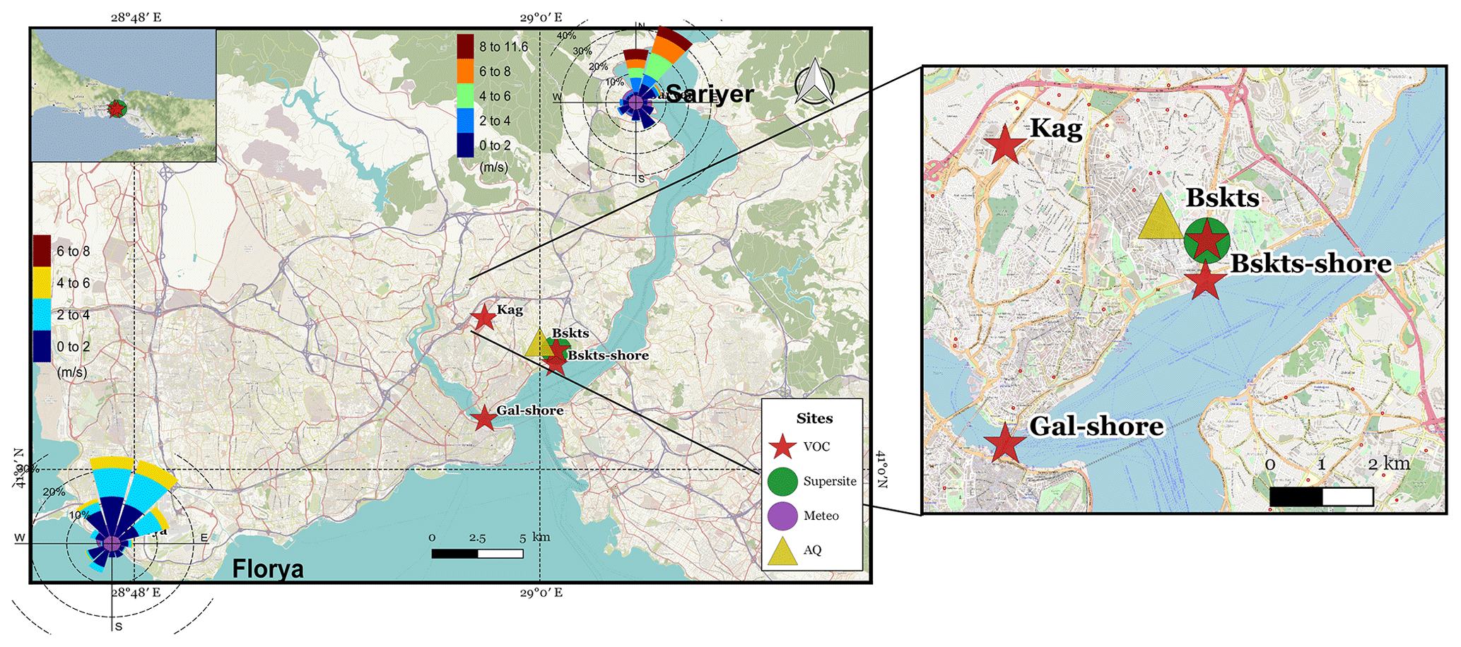
Figure 1Different measuring sites during the TRANSEMED campaign: Besiktas (Bskts), Kagithane (Kag), Galata (Gal), Florya (Flo), and Sarıyer (Sar) and wind roses at Florya and Sarıyer stations. Map: ©OpenStreetMap contributors 2015. Distributed under a Creative Commons BY-SA License (OpenStreetMap contributors, 2015).
The urban site (labeled as a super site in Fig. 1) is located along the Barbaros Boulevard (Blvd) in the district of Besiktas in Istanbul, Turkey (41∘02′33 N, 29∘00′26 E), on the European shore of the Bosporus strait. Barbaros Blvd is a high-traffic-density street, which is a major route between the city center (a.k.a. “historical peninsula”) and the Bosporus Bridge that connects Asia and Europe. The Besiktas district is also expected to be impacted by the mixture of major anthropogenic emissions (Markakis et al., 2012). Note that the sampling site was 500 m away from the Besiktas Pier (Bsks-shore in Fig. 1) and the Bosporus strait is 4 km away from the Haydarpasa Port. Dense industrial areas like Ikitelli are located in the southwestern part of the city 20-km away from Besiktas. Trace gas measurements including VOCs were conducted at the super site from 14 to 30 September 2014 (during the non-heating season). In parallel, punctual VOC sampling at four other locations has been performed to assess the spatial variability of VOC composition and to support the interpretation of PMF factors. Punctual sampling included one residential area in the district of Kagithane (Kag – 29 and 30 September 2014), one roadside site on the Barbaros Blvd (Bskts – 24 September 2014), two seashore sites at the Besiktas pier (Bskts-shore 26 September 2014), and on the Galata Bridge (Gal-shore 29 September 2014). Local ferries that connect the European and Asian sides continuously travel to the Besiktas pier with a few minutes parking time at berth. The Galata Bridge spans the Golden Horn in Istanbul with a roadway on its upper part. For data analysis the Istanbul Metropolitan Municipality provided air quality data (CO, NOx, and SO2) from its Basiktas site (Fig. 1), and meteorological data were obtained from Turkish State Meteorological Office (wind speed, wind direction, temperature, relative humidity, and ambient pressure) from its network (Sarıyer and Florya stations in Fig. 1).
2.2 VOC instrumentation
The online instrumentation for VOCs at the super site included an airmoVOC GC–FID (gas chromatograph and flame ionization detector, Chromatotec®) and a high-sensitivity PTR-MS (proton transfer reaction mass spectrometer, Ionicon®) at 30 and 5 min time resolution, respectively. Principle, performances, and operation conditions of both instruments have been described elsewhere (Gaimoz et al., 2011; Borbon et al., 2013; Ait-Helal et al., 2014).
Ambient air sampling was performed at the height of 2 m a.g.l. Air was pulled through two independent 3 m Teflon lines (PFA, 1∕4 in. outside diameter) towards the instruments. During the TRANSEMED campaign, the GC–FID measured 15 VOCs from C4 to C8 (alkanes, alkenes, aromatics). VOC-free zero air and a certified parts-per-billion-level gaseous standard from NPL (National Physical Laboratory, UK) at 4±0.8 ppb were injected every 3 d. A total of 11 protonated masses were monitored with the PTR-MS. The background signal was determined every 2 d for 30 min by passing air through a catalytic converter containing platinum-coated pellets heated to 320 ∘C. The drift pressure was maintained at 2.20 mbar and the drift voltage at 600 V. The primary H3O+ ion counts at m∕z 21 ranged between 0.9×10⁷ and 1.4×10⁷ cps with a contribution from the monitored first water cluster at m∕z 37 < 5 %. Two multipoint calibrations were performed using a gas calibration unit (GCU) and a standard mixture of 17 species (Ionimed Analytik GmbH, Innsbruck, Austria) before and after the campaign over a 0.1–20 ppb range; the linearity was higher than 0.99 (R2). The species used for the calibration were methanol (contributing m∕z 33), acetaldehyde (m∕z 45), acetone (m∕z 59), isoprene (m∕z 69), crotonaldehyde (m∕z 71), 2-butanone (m∕z 73), benzene (m∕z 79), toluene (m∕z 93), and α-pinene (m∕z 137). In addition, five regular 5 ppb control points were carried out during the campaign. Except m∕z 33 (17 %), the standard deviation of the calibration coefficients lay between 3 % (m∕z 93) and 9 % (m∕z 42). The NPL standard was used to cross-check the quality of the calibration and to perform regular one-point calibration control for isoprene and C6–C9 aromatics (4.0±0.8 ppb). A relative difference of less than 10 % was found between both standards. The mean calibration factor for all major VOCs is derived from the slope of the mixing ratios of the diluted standards with respect to product ion signal normalized to H3O+ and H3O+H2O. Calibration factors ranged from 2.54 (m∕z 137) to 19.0 (m∕z 59) normalized counts per second per part per billion by volume (ncps ppbv−1). Linearly interpolated normalized background signals are subtracted to the normalized signal before applying the calibration factor to determine ambient mixing ratios. Detection limits were taken as 2σ of the normalized background signal divided by the normalized calibration factor. Detection limits lay between 50 ppt (e.g., monoterpenes) and 790 ppt (methanol). Finally 11 protonated target masses have been monitored here: methanol (m∕z 33.0), acetonitrile (m∕z 42.0), acetaldehyde (m∕z 45.0), acetone (m∕z 59.0), methyl vinyl ketone (MVK) and methacrolein (MACR) (m∕z 71.0), benzene (m∕z 79.0), toluene (m∕z 93.0), C8 aromatics (m∕z 107.0), C9 aromatics (m∕z 121.0), and terpenes (m∕z 137.0). While Yuan et al. (2017) reports interferences in their review paper (Yuan et al., 2017) for some of these protonated masses they can be excluded in a high-NOx environment like the Istanbul megacity.
Off-line instrumentation, which included sorbent tubes and canisters, provides a lighter setup to describe emission source composition and the spatial variability of VOC composition to support the PMF analysis. The instrumentation was deployed at the super site and at the four locations reported in Fig. 1 (VOC label). Off-line measurements of C5 to C16 NMHCs (alkanes, aromatics, alkenes, aldehydes) were performed using multibed sorbent tubes of Carbopack B & C (Sigma-Aldrich Chimie S.a.r.l., Saint-Quentin-Fallavier, France), at a 200 mL min−1 flow rate for 2 h using a flow-controlled pump from GilAir. Samples were first thermodesorbed and then analyzed by TD-GC–FID-MS within 1 month after the campaign. The sampling and analysis methods are detailed elsewhere (Detournay et al., 2011). Air samples were also collected by withdrawing air, for 2–3 min, into preevacuated 6 L stainless-steel canisters (14 samples) through a stainless-steel line equipped with a filter (pore diameter = 2 µm) installed at the head of the inlet. Prior to sampling, all canisters were cleaned at least five times by repeatedly filling and evacuating zero air. Tubes and canisters were sent back to the laboratory (Salameh et al., 2014). The frequency of off-line samplings is reported in Fig. S1 in the Supplement at the various sites reported in Fig. 1.
The compounds commonly measured by online and off-line techniques, namely aromatics, isoprene, pentanes, and terpenes, were used to cross-check the quality of the results at the super site on 26 and 29 September. The comparison is provided in Fig. S2 in the Supplement. The variability between PTR-MS and airmoVOC is highly consistent (R2>0.85), and the differences in concentrations do not exceed ±22 %. While the number of off-line samples is limited (five samples), the values are consistent. The pentanes, terpenes, and C9 aromatics collected by tubes or canisters are also compared to airmoVOC (Fig. S3). Most of the data compare well at ±20 % with a few exceptions that do not exceed ±50 %. Finally, the correlation between PTR-MS and airmoVOC is surprisingly weak for isoprene. Despite some interferences like furans not being excluded for m∕z 69 with PTR-MS (Yuan et al., 2017), the good correlation between m∕z 69 from PTR-MS and ambient temperature led to the use of the PTR-MS data for isoprene.
2.3 Other instrumentation
At the super site, other trace gases like carbon monoxide (CO) and NOx (NO+NO2) have been performed on a 1 min basis. NOx was monitored by the Thermo Scientific model TEI 42i instrument, which is based on chemiluminescence and NO2-to-NO conversion by a heated molybdenum converter. The NOx analyzer was installed after 25 September at the super site. CO was monitored by the Horiba APMA-370 instrument model, which is based on the non-dispersive infrared (NDIR) technique. Basic meteorological parameters (wind speed and direction, temperature, relative humidity, and atmospheric pressure) were measured on a 1 min basis. Air quality data with additional sulfur dioxide (SO2) and meteorological data from other stations operated by the Istanbul Metropolitan Municipality have also been used to test the consistency of our data and to support PMF interpretation (see Fig. 1 and Sect. 1.1).
In addition to gaseous and meteorological parameters, particulate matter samples were also collected at the site. A Partisol PM2.5 sequential sampler (Thermo Scientific, USA) was deployed (24 h between 28 August and 13 November 2014 and every 6 h until 28 January 2015), and collected samples were analyzed in terms of metals by inductively coupled plasma mass spectrometry (ICPMS). Moreover, a Tecora PM10 sampler (Italy) was used to collect daily PM10 samples (30 August 2014–3 February 2015) and collected samples were analyzed in terms of EC and OC by means of a Sunset Lab (Oregon, USA) thermal optical analyzer, molecular organic markers using GC-MS (Varian CP 3800 GC equipped with a TR-5MS fused silica capillary column), and water-soluble organic carbon (WSOC) by means of an organic carbon analyzer (TOC-VCSH, Shimadzu). The sampling time and availability of the data are reported in Fig. S1 of the Supplement.
2.4 Positive matrix factorization (PMF)
2.4.1 PMF description
The U.S. EPA PMF 5.0 model was used for VOC source apportionment. The method is described in detail in Paatero and Tapper (1994), Paatero (1997), and Paatero and Hopke (2003).
The general principle of the model is as follows: any matrix X (input chemical dataset matrix) can be decomposed in a factorial product of two matrixes G (source contribution) and F (source profile) and a residual part not explained by the model E. Equation (1) summarizes this principle in its matrix form:
where i is the number of observations, j the number of the measured VOC species, and k the number of factors.
The goal of the PMF is to find the corresponding non-negative matrixes that lead to the minimum value of Q.
where fkj≥0 and gkj≥0 and where n is the number of samples, m the number of considered species, and sij an uncertainty estimate for the jth species measured in the ith sample.
2.4.2 Preparation of input data
Two input datasets (or matrixes) are required by the PMF: the first one contains the concentrations of the individual VOC and the second one contains the uncertainty associated with each concentration.
The VOC input dataset combines data from both the PTR-MS and the GC–FID. The PTR-MS data have been synchronized with the ones from the GC–FID on its 20 min sampling time every 30 min. The final chemical database used for this study comprises a selection of 23 hydrocarbons and masses divided into seven compound families: alkanes (isobutane, n-butane, n-hexane, n-heptane, isopentane, n-pentane, and 2-methyl-pentane), alkenes (1-pentene, isoprene, and 1,3-butadiene), aromatics (ethylbenzene, benzene, toluene, (m + p)-xylenes, o-xylene, and C9 aromatics), carbonyls (methyl ethyl ketone (MEK), methacroleine + methyl vinyl ketone (MACR + MVK), acetaldehyde, and acetone), alcohol (methanol), nitrile (acetonitrile), and terpenes. Alkanes and alkenes were measured by the GC–FID while benzene, toluene, isoprene, C8 aromatics, carbonyls, alcohol, nitrile, and terpenes were the ones measured by the PTR-MS. For benzene, toluene, and C8 aromatics the PTR-MS data were selected because of the smallest number of missing data.
Since the PMF does not accept missing values, missing data must be replaced. The percentage of missing values ranges from 8 % to 79 % for species measured by the GC–FID. Butanes (iso/n), pentanes (iso/n), and (m + p)-xylenes have the lowest missing value percentage (ranging from 8 % to 12 %) while o-xylene (30 %), 2-methyl-pentane (32 %), ethylbenzene (42 %), 1-pentene (62 %), n-hexane (66 %), n-heptane (72 %), and 1,3-butadiene (79 %) have the highest percentage of missing values. There were only two missing values (0.33 %) for species measured by the PTR-MS.
For those species with a proportion of missing values below 40 %, missing data were replaced by a linear interpolation. For species with a proportion of missing data exceeding 40 %, each missing data point was substituted with the median concentration over the whole measurement period. All the concentrations were above the detection limit.
The uncertainty σij associated with each concentration (Eq. 3) is determined using the method developed within the ACTRIS (Aerosol, Cloud and Trace Gases Research Infrastructure) network (Hoerger et al., 2015) and used in Salameh et al. (2016):
This uncertainty considers the different sources of uncertainty affecting the precision and the accuracy terms. The precision is associated with the detection limit of the instrument and the repeatability of the measurement, while the accuracy includes the uncertainty of the calibration standards and the dilution when needed.
The uncertainty of the PTR-MS ranges between 5 % (toluene) and 59 % (acetaldehyde) of the concentrations while the uncertainty for the GC–FID ranges between 4 % (2-methyl-pentane) and 17 % (o-xylene) of the concentration. Further information about the uncertainties calculation are found in Sect. S1 of the Supplement.
2.4.3 Determination of the optimal solution
The objective of the PMF is to determine the optimal number of factors (p) based on several statistical criteria. Several base runs were performed with a different number of factors from 2 to 12. Statistical criteria were then used to determine the appropriate p value such as Q (residual sum of squares), IM (maximum individual column mean), IS (maximum individual column standard deviation) as defined by Lee et al. (1999), and R2 (indicator of the degree of correlation between predicted and observed concentrations). Q, IM, IS, and R2 are then plotted against the number of factors (from 2 to 12) (Salameh et al., 2016). The number of chosen factors corresponds to a significant decrease in Q, IM, and IS. In our study, an optimal solution of five factors was retained. In order to ensure the robustness of the solution, a Fpeak value of −1 was set by considering the highest mean ratio of the total contribution vs. the model as well as the numbers of independent factors (Salameh et al., 2016).
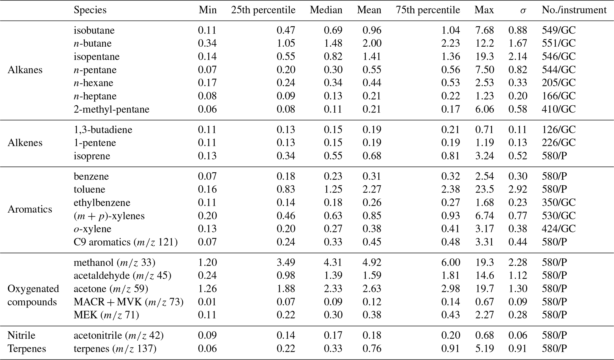
Table 1Statistical summary of VOC concentrations (ppbv) measured at the urban site of Besiktas from 17 to 30 September. The initials no., GC, P, T, and C stand for the number of samples and instruments measured by the GC–FID, PTR-MS, tubes, and canisters.
2.4.4 PMF reference run
A PMF reference run has been performed by removing the period during which there were no GC–FID data (night from 24 to 25 September). In addition, these datasets have been chosen as the PMF reference run because of the higher correlation between observed and reconstructed data by the PMF model (see also Sect. 3.2). A good correlation (R2=0.97) between total reconstructed VOC and measured VOC was obtained. For most compounds the variability is reproduced well with a R2 usually higher than 0.70. Poorer correlation was found for alkenes (1-pentene (R2=0.55), 1,3-butadiene (R2=0.22), and isoprene (R2=0.57)) as well as for n-hexane (R2=0.09), MEK (R2=0.41), and acetaldehyde (R2=0.32). The R2 of the contribution of the five factors between each other has been calculated; it was found that the value of R2 does not exceed 0.28 and is usually less than 0.05, indicating the statistical independence of the five factors. There is therefore no significant correlation between the factors, which means that the factors are independent.
The PMF output uncertainties were estimated by three models: the DISP model (base model displacement error estimation), the BS model (base model bootstrap error estimation), and the DISP + BS model. Further information for the estimation of model prediction uncertainties can be found in Norris et al. (2014) and Paatero et al. (2014). The DISP results of the PMF run show that the five-factor solution is stable and sufficiently robust to be used because no swaps occurred. All the factors were reproduced well through the BS technique at 100 % for factor 1, 96 % for factor 2, 100 % for factor 3, 99 % for the factor 4, and 100 % for factor 5; there were not any unmapped runs. The DISP + BS model shows that the solution is well constrained and stable.
2.4.5 Sensitivity tests to evaluate PMF results
The sensitivity of PMF results to input data has been tested in order to evaluate the representativeness of the PMF reference run results. These tests evaluate the effect of some time period selection described in Sect. 3 (periods 1, 2, and 3, nighttime peaks) and the incorporation of species with a high number of missing data as well as a test where all missing data were directly replaced by the median of species over all the measurement period instead of interpolation.
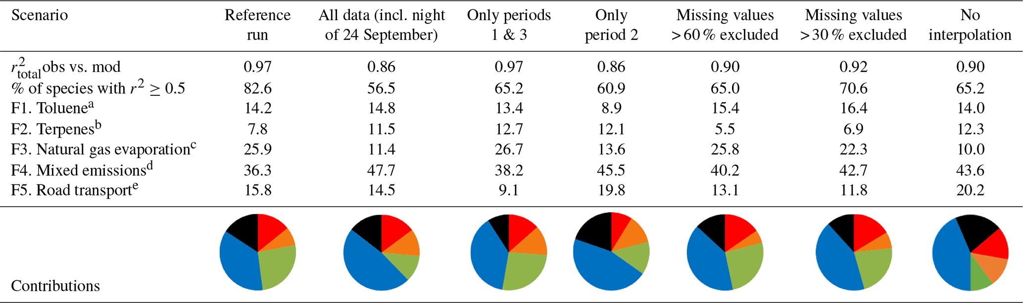
Table 2Contributions of each factor to each sensitivity test (as a percentage).
a Displayed in red. b Displayed in orange. c Displayed in green. d Displayed in blue. e Displayed in black.
Table 2 summarizes the contribution of each factor for every sensitivity scenario as well as the values of the correlations between observed and modeled concentrations. The reference run has the best fit with , and more than 82 % of species were reconstructed well by the PMF (r2≥0.5). While the sensitivity tests do not perform as well statistically as the reference run, they all show that the same factors are extracted even though the relative contributions could be slightly modified by ±16 %. Factors will be discussed in Sect. 3.3.
2.5 FLEXPART model
FLEXPART is a Lagrangian particle dispersion model and is widely used to stimulate atmospheric transport. It gives information about long-range and mesoscale dispersion of air pollutants such as air mass origin (back trajectories) (Brioude et al., 2013). FLEXPART was driven by ECMWF analysis (at 00:00, 12:00 UTC) and the 3 h forecast fields from the operational European Centre for Medium-Range Weather Forecasts – Integrated Forecast System (ECMWF-IFS). To compute the FLEXPART trajectories, the ECMWF meteorological fields were retrieved at 0.25∘ resolution and 91 vertical levels. The FLEXPART output is reported in Fig. 2.
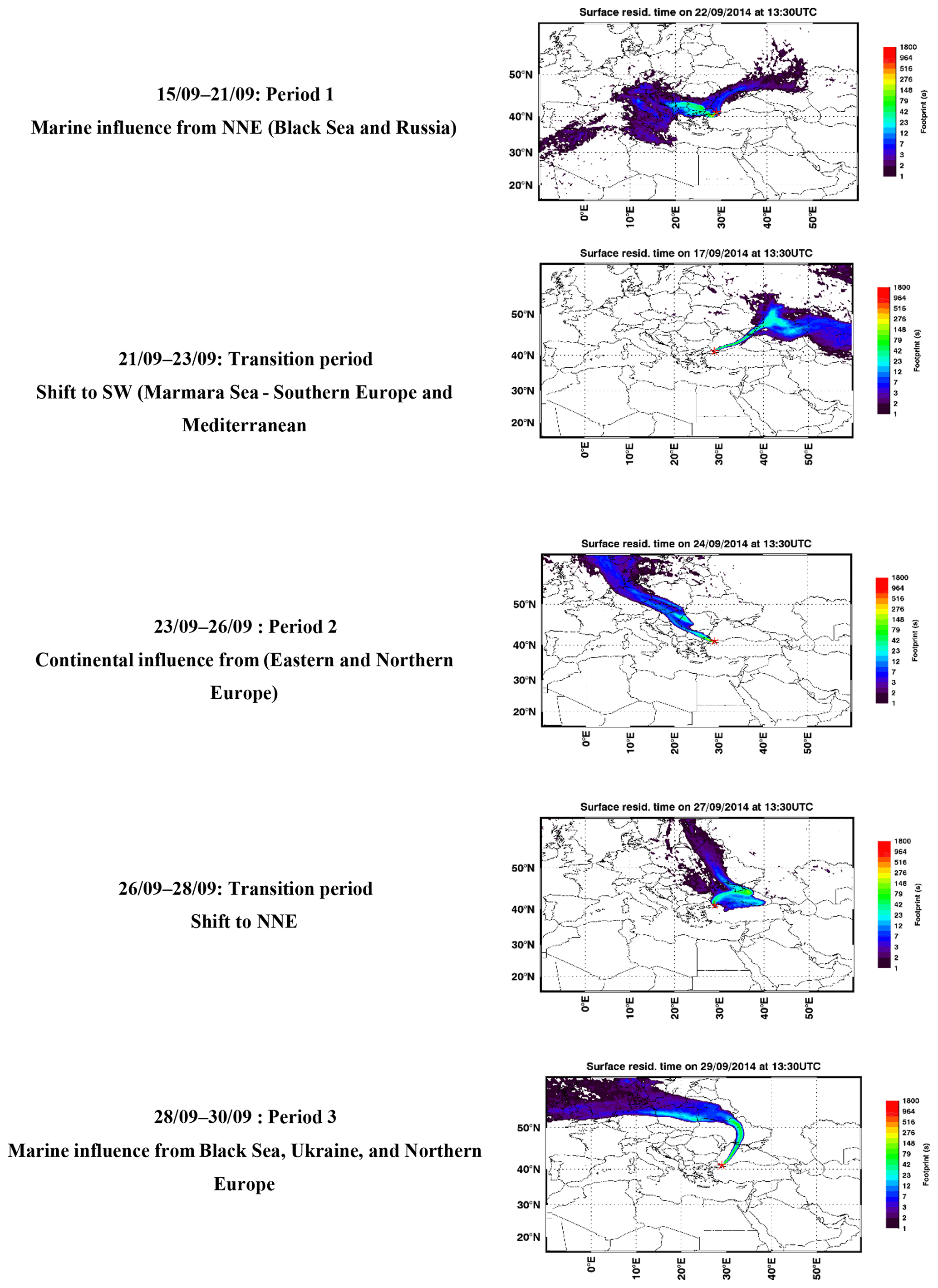
Figure 2Surface residence time of representative air mass trajectories from the FLEXPART model during the TRANSEMED Istanbul campaign.

Figure 3Variations in meteorological parameters at the super site of Besiktas. Wind speeds were recorded at the stations of Florya and Sarıyer. Wind direction displayed in this figure was recorded at the station of Sarıyer. Periods 1 and 3 are in blue, transition periods are in white, and period 2 is in grey.
3.1 Meteorological conditions and air mass origin
The time series of meteorological parameters are reported in Fig. 3. Based on in situ observations and FLEXPART simulations (Fig. 2), the meteorological situation has been divided into three types of periods.
-
Periods 1 and 3 from 15 to 21 and from 28 to 30 September with marine air masses coming from the Black Sea and Russia and/or Ukraine and northern Europe (Fig. 2). During period 1, in situ temperature and relative humidity were characterized by a clear and opposite diurnal cycle while no cycle is depicted during period 3. During both periods relative humidity is high with two rain events (18 and 28 September). Relative humidity is high during the night (80 %) while temperature is high during the day (from 14.7 to 27.6 ∘C with an average of 21.2 ∘C). Wind speeds are the highest (> 3 m s−1 in Besiktas and up to 12 m s−1 at Sarıyer) with a northern wind direction.
-
Period 2 from 23 to 26 September with continental air masses coming from eastern and northern Europe (Fig. 2). Locally wind direction is variable. Temperature and relative humidity were characterized by the same diurnal cycles as in Period 1. Temperature decreased, ranging between 11.8 and 25.4 ∘C with an average of 17.9 ∘C. Lower wind speeds were recorded (3.1 m s−1 in Besiktas and up to 6 m s−1 in Sarıyer). Wind direction varied between WSW (west-southwest) and SSE (south-southeast) and between the north and ENE (east-northeast).
-
A first transition period between periods 1 and 2 (21 to 23 September) showed a wind direction shift towards the southern sector (Marmara Sea) (Fig. 2). Wind speed recorded the lowest values (< 1.3 m s−1 in Besiktas and < 5 m s−1 in Sarıyer). It rained on 23 September. A second transition period between periods 2 and 3 (from 26 to 28 September) showed a wind direction shift toward the NNE (north-northeast) (Fig. 2). On 6 September, the temperature increased to 26 ∘C. It rained from the night of 26 September until the end of the period during which temperature decreased to 14.7 ∘C. This period was also characterized by higher wind speed (up to 9 m s−1 in Sarıyer and 2.7 m s−1 in Besiktas) coming from the ESE (east-southeast) and north.
3.2 VOC distribution
3.2.1 Ambient concentration level and composition
Observed VOCs at the super site of Besiktas are representative of the ones usually encountered at urban background sites. Biogenic compounds are isoprene and terpenes while anthropogenic compounds include both primary (alkanes, alkenes, aromatic compounds) and secondary compounds (oxygenated VOC).
Statistics on the VOC concentrations measured by GC–FID and PTR-MS at the super site of Besiktas are reported in Table 1. VOCs show a high temporal variability with maxima reaching several tens of parts per billion (isopentane, ethylbenzene, methanol, and acetone). Most VOC median concentrations are below 1 ppb except for n-butane (1.48 ppb), toluene (1.25 ppb), and some oxygenated compounds like acetaldehyde (1.39 ppb) and acetone (2.33 ppb). The average composition of VOCs mainly includes OVOCs (0.12–4.92 ppb), which represent 43.9 % of the total VOC (TVOC) observed mixing ratio, followed by alkanes (0.21–2.00 ppb; 26.33 %), aromatic compounds (0.26–2.27 ppb; 20.66 %), alkenes (0.19–0.68 ppb; 4.81 %), terpenes (3.44 %), and acetonitrile (0.84 %). Both OVOCs and alkanes contribute up to 70.2 % of the TVOC concentrations. Methanol (22.40 %, 4.92 ppb on average) is the main oxygenated compound measured in this study, followed by acetone (11 %, 2.63 ppb). N-butane (9.11 %, 2.00 ppb) and isopentane (6.43 %, 1.41 ppb) are the two major alkanes. Toluene is the most abundant aromatic compound (50 %, 2.27 ppb). This was the case for most of the previous VOC studies performed in Istanbul (Demir et al., 2011; Kuntasal et al., 2013; Muezzinoglu et al., 2001; Bozkurt et al., 2018; Elbir et al., 2007).
Levels of alkanes, some alkenes, and aromatics are compared to levels in other European megacities: Paris and London (Borbon et al., 2018) at both urban and traffic sites as well as at an urban site in Beirut (Salameh et al., 2015) during summer (Fig. S4 in the Supplement). Consistency in urban hydrocarbon composition worldwide has already been observed (Borbon et al., 2002; von Schneidemesser et al., 2010; Dominutti et al., 2016). Despite differences in absolute levels, the hydrocarbon composition in Istanbul is quite similar to that in the other cities. Beirut has the highest concentrations of n-butane, isopentane, and 2-methyl-pentane. Higher concentrations in toluene and (m + p)-xylenes were found in Paris, Beirut, and Istanbul. Such a similarity would suggest that the same sources control the hydrocarbon composition, especially traffic in all cities including Istanbul (see also Sect. 3.3 on PMF).
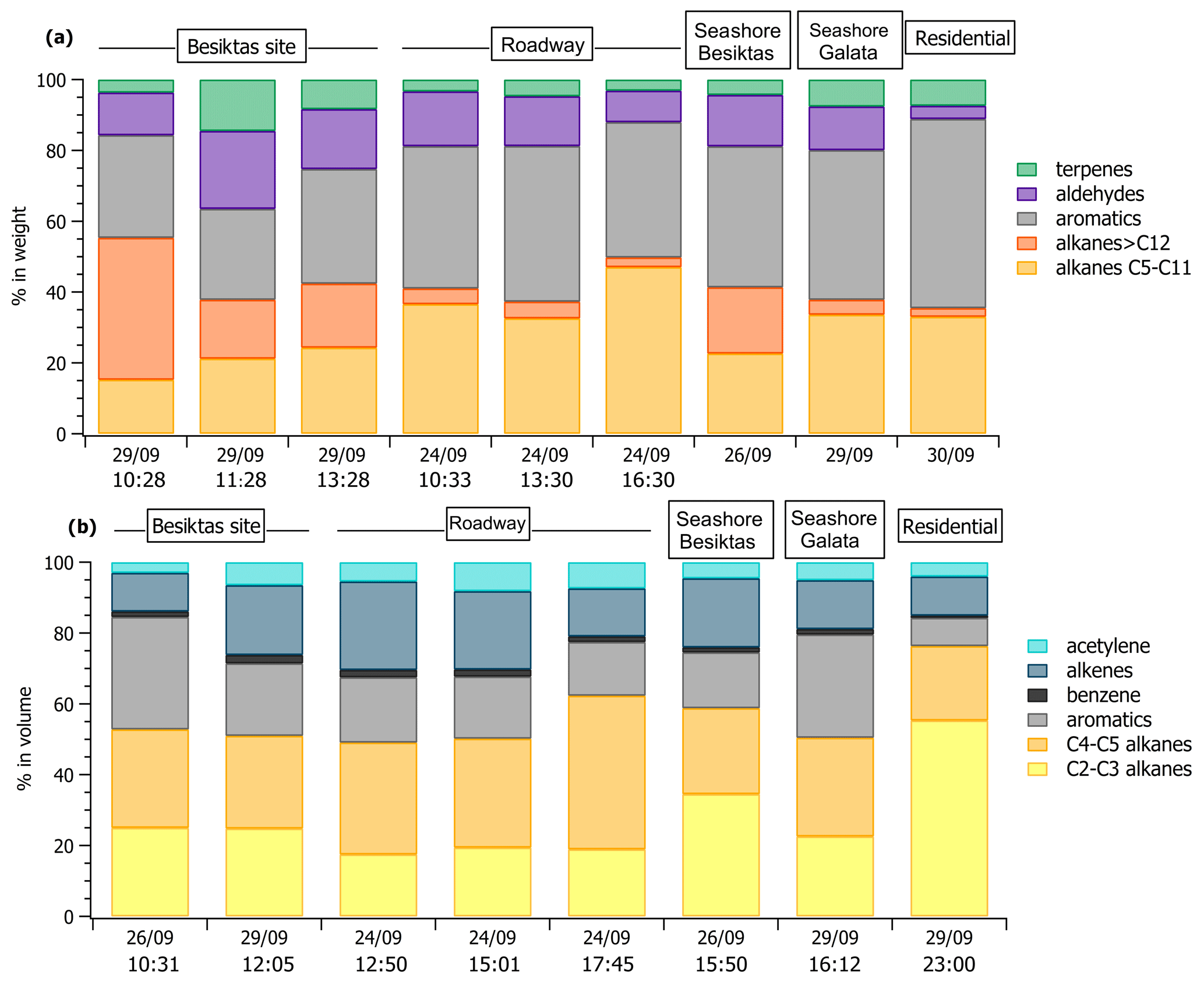
Figure 4VOC composition at various locations in Istanbul from tubes (a) and canister (b) sampling.
Off-line VOC concentrations collected with tubes are reported in Table S5 in the Supplement at various locations including the Besiktas super site. While the number of samples is limited in time, off-line measurements provide a general picture of a wider spectrum of VOCs that are not measured at the super site like light hydrocarbons (C2–C3 alkanes and alkenes), C6–C11 carbonyls, speciated terpenes (camphene, limonene, β-pinene), and C12–C16 intermediate-volatility organic compounds (IVOCs). Therefore, these datasets allow us to address the spatial variability of VOC concentrations and composition within the megacity. The comparison of concentrations between different areas is limited because of the different sampling times. Therefore, the analysis only focuses on VOC relative composition. The relative composition divided into major VOC chemical groups at each site by sorbent tubes and canisters is reported in Fig. 4a and b, respectively. The composition is variable across the megacity for the aliphatic fraction of high- and intermediate-volatility hydrocarbons (C2–C16). As expected, the composition of the 29 September 12:05 UTC+3 (for all times throughout) sample at the Besiktas site is like that derived from the roadside measurements, highlighting the influence of road transport emissions at the super site. Interestingly, the VOC composition of the three samples from sorbent tubes at the Besiktas site are different from the ones at the roadway site with a higher proportion of IVOCs. The VOC composition of the 26 September 10:31 sample by canister is rather similar to that from the seashore sample in Galata (29 September 16:12 sample). In the same way the VOC composition of the samples at the super site derived from tubes is rather like that of the Besiktas seashore. For both of them, the proportion of IVOCs is significant (from 15 % to 40 % in weight). While light VOCs are expected to be of minor importance when considering ship emissions, the higher presence of heavier organics is however expected as observed for alkanes by Xiao et al. (2018) in ship exhaust at berth. The VOC composition comparison would thus suggest not only the impact of road traffic emissions on their composition but also the potential impact of local ship traffic emissions. Finally the composition at Besiktas is not affected by residential emissions, which are enriched in light C2–C3 alkanes (canisters) or aromatics (canisters).
3.2.2 Time series and diurnal variations
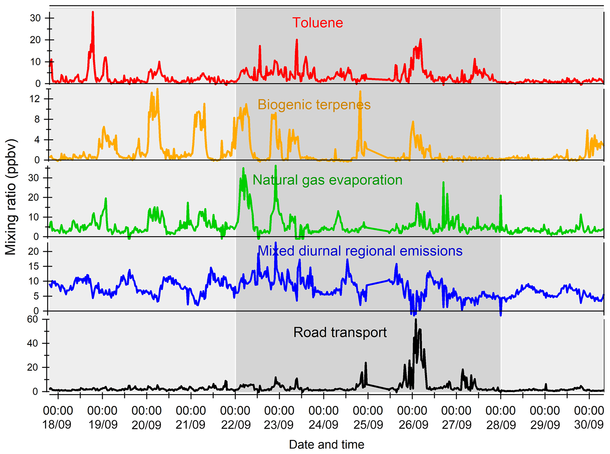
The variability of VOC concentrations is driven by several factors: emissions (anthropogenic or biogenic), photochemical reactions (especially with the OH radical during the day and ozone and nitrates at night for alkenes), and the dynamics of the atmosphere (including dilution due to the height of the boundary layer) (Filella and Peñuelas, 2006). The time series of inorganic trace gases (NOx and CO) and some VOCs representing the diversity of sources and reactivity are reported in Fig. 5. The meteorological periods 1, 2, and 3 described in the previous Sect. 3.1 are also indicated. Because NOx at the super site was only measured from 25 to 30 September, data from the air quality station in Besiktas were used (see Fig. 1). One should note that the time series of NOx at the super site and at the Besiktas station are consistent.
Time series of NOx and CO show high concentrations but a different pattern regardless of the origin of air masses. While a daily cycle of NOx is depicted, CO does not show any clear pattern. The NO2∕NOx ratio fluctuates between 0.34 and 0.93 with an average and median value of 0.53 and 0.55, respectively. These values are very high compared to what is usually found in the literature (Grice et al., 2009; Kousoulidou et al., 2008; Keuken et al., 2012), which is mostly low and below 0.50. However higher values of the NO2∕NOx ratio can be found in diesel passenger cars (Grice et al., 2009; Vestreng et al., 2009) and vans (Kousoulidou et al., 2008). This ratio would reflect the impact of the combustion of heavy fuels in a megacity. After road transport, cargo shipping is the second highest contributor to NOx levels according to the local/regional inventory (Markakis et al., 2012).
Anthropogenic VOC time series (benzene, isopentane, and isobutane) exhibit a high-frequency variability but usually show higher concentrations during the night, especially during period 2. One cause is the very low wind speeds at night, especially during period 2 (Fig. 3), which would reinforce the accumulation of pollutants. Under marine influence (periods 1 and 3), VOC concentrations are the lowest, especially during period 3, which is characterized by rainy days (27 and 28 September), high wind speed, and colder temperatures (Fig. 5). These conditions favor atmospheric dispersion. During transition periods and under continental influence (period 2), VOC concentrations exhibit a strong day-by-day variability with episodic nocturnal peaks in particular on 25 and 26 September. While these peaks are not always concomitant between VOC and are not associated with any increase in NOx and CO levels, they occur under south and southwestern wind regimes, which are unusual wind regimes according to Fig. 1. This points out the potential influence of industrial and port activities other than fossil fuel combustion. For instance, maximum concentrations of butanes occurred during the period of the marine–continental regime shift with the well-established southwestern wind regime on 22, 23, and 26 September at the end of the day. Maximum concentrations of pentanes occurred during the night of 26 to 27 September like for aromatics (e.g., benzene) (Fig. 5).
Except during transition periods, the background levels of measured trace gases are not affected by the origin of air masses. This strongly suggests that the pollutants measured during TRANSEMED Istanbul were from local and regional sources. Finally, time series would suggest the influence of multiple local and regional sources other than traffic on VOC concentrations, likely industrial and/or port activities, at the super site.
Isoprene and its oxidation products (MACR + MVK) covariate most of the time in periods 1 and 3. They usually show their typical diurnal profiles with higher concentrations during the warmest days and at midday due to biogenic emission processes. Their significant correlation with temperature (R=0.7) implies emission from biogenic sources. Around the Besiktas site, 49.5 % of the vegetation is occupied by hardwood and hardwood mix trees while only 6 % is occupied by softwood and hardwood mix trees. While Quercus (isoprene emitter) only occupies 7.7 % of the total vegetation coverage (Ministry of Forestry, personal communication, 2018), the presence if isoprene at the super site is probably due to the surrounding trees.
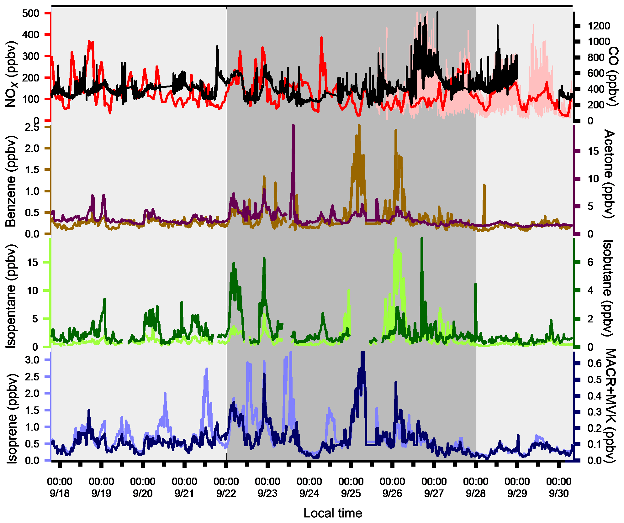
Figure 5Time series of NOx, CO, and a few VOCs. Background colors represent the different periods relative to meteorological conditions (light grey for periods 1 and 3 and dark grey for period 2). Time series of NOx data from the super site are in pink and the ones from the Besiktas site are in red.
Except during transition periods, the background levels of measured trace gases are not affected by the origin of air masses. The background levels stay constant under continental or marine influence and regardless of the atmospheric lifetime of the species. This strongly suggests that the pollutants measured during TRANSEMED Istanbul were from local and regional sources. Finally, time series would suggest the influence of multiple local and regional sources other than traffic on VOC concentrations, likely industrial and/or port activities, at the super site.
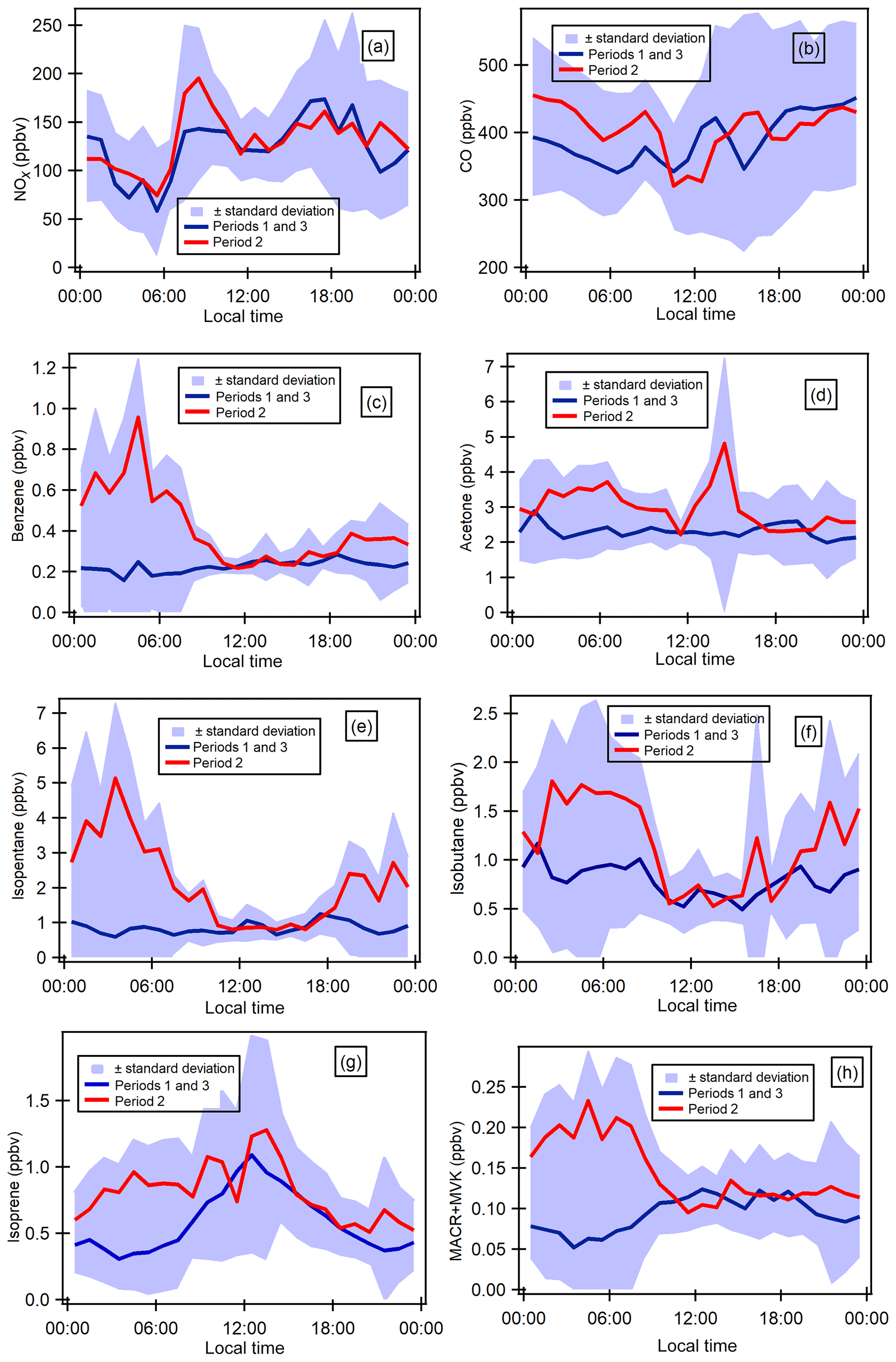
Figure 6Diurnal profiles of some selected gaseous species (ppbv). Blue shaded areas represent the minimum and maximum diurnal concentrations over all the measurement periods, and blue lines show the average diurnal concentrations during periods 1 and 3 and red lines the average concentrations during period 2.
Taking into consideration time series variability, diurnal variations have been split into periods 1 and 3 and period 2 for selected VOCs as well as two combustion-derived trace gases (NOx and CO). Diurnal profiles of atmospheric concentrations are reported in Fig. 6. Local traffic counts for road transport (personal communication from Istanbul Municipality for fall 2014) and shipping (https://www.marinetraffic.com/en/ais/details/ports/724/Turkey_port:ISTANBUL, 14 January 2019) are also reported in Fig. S6 in the Supplement. Maritime traffic is mostly for passenger shipping (58.02 %) compared with 16 % for cargo shipping. The diurnal profiles of ship and road traffic counts are similar.
Generally, concentrations during period 2 are higher than the ones during periods 1 and 3 and show different diurnal patterns for some compounds. The profile of NOx is consistent with the one of traffic counts (Fig. S6 of the Supplement). NOx exhibits higher concentrations during the day and lower concentrations at night for both periods with a morning peak (07:30–08:30) and one early evening peak from 17:30 (Fig. 6a). This is typical of traffic-emitted compounds with morning and evening rush-hour peaks as observed in many other urban areas like Paris, France, in Europe (Baudic et al., 2016) or Beirut, Lebanon, in the eastern Mediterranean (Salameh et al., 2016). As already depicted in time series, the CO diurnal profile is different from that of NOx. CO concentrations show higher concentrations in the late evening and lower concentrations during the day. During the day, CO is also characterized by a double peak: one in the morning (08:30) and the other one in the middle of the day (Fig. 6b). Both NOx and CO show quite similar diurnal profiles between the three periods even if morning concentrations tend to be higher.
VOCs show different profiles from that of NOx. Under marine influence (periods 1 and 3), primary anthropogenic VOCs (i.e. benzene, alkanes, and other aromatics) almost exhibit a constant profile while they show a higher concentration from midnight until 10:00 under continental influence (period 2). For instance, benzene (Fig. 6d) and isopentane (Fig. 6f) nighttime concentrations increase by 4-fold compared to the levels under marine influence. In the middle of the day, the concentration levels are the same as during periods 1 and 3. The profiles of primary anthropogenic VOCs show the complex interaction between local and regional emissions and dynamics. Period 2 shows the influence of VOC emissions other than traffic and combustion processes (no effect on NOx and CO) at night. While the influence of traffic emissions on CO and VOC cannot be excluded; it seems that their emission level is not high enough to counteract the dispersion effect during the day unlike NOx. This will be further investigated in the PMF analysis.
Isoprene concentrations increase immediately at sunrise and decrease at sunset during periods 1 and 3 (marine influence), which indicates its well-known biogenic origin (Fig. 6g), which is light and temperature dependent. Isoprene and MACR + MVK concentrations increase at night during period 2 like other alkanes and aromatics, suggesting their potential anthropogenic influence.
Provided some interferences like furans could contribute to isoprene signal by PTR-MS measurements (Yuan et al., 2017), this would suggest an anthropogenic origin for isoprene. While the signals of m∕z 71 are commonly attributed to the sum of MVK and MACR, which are both oxidation products of isoprene under high-NO conditions, more recent GC-PTR-MS studies identified some potential interferences for MVK and MACR measurements, including crotonaldehyde in biomass-burning emissions, C5 alkenes, and C5 or higher alkanes in urban regions (Yuan et al., 2018). Such interferences cannot be ruled out here. During periods 1 and 3, MACR + MVK concentrations follow the same general pattern as isoprene.
With a relatively long atmospheric lifetime (≈68 d), acetone's concentration is quite constant throughout the day within period 1, with a peak in the middle of the day and lower concentrations during the night for period 2 (Fig. 6c). The peak in the middle suggests the presence of a secondary origin. Acetone can have both primary and secondary sources (Goldstein and Schade, 2000; Macdonald and Fall, 1993). Methanol and MEK have the same general pattern as for acetone during both periods without the peak in the middle of the day, suggesting that they might have the same emission source.
3.3 PMF results
3.3.1 Factor identification
The factor profiles have been analyzed using the variability of their contribution together with several external variables (NOx, SO2, CO, meteorological parameters, emission profiles). PMF factors are displayed in Fig. 7. The time series and diurnal profiles of their contributions are displayed in Figs. 8 and 9, respectively.
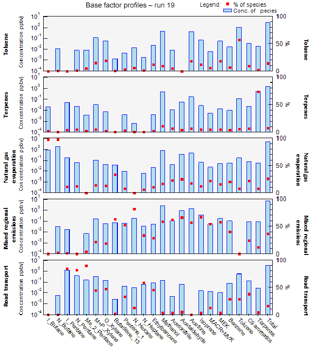
Figure 7Source composition profiles of the PMF factors. The concentrations (ppbv) and the percent of each species apportioned to the factor are displayed as a pale blue bar and a red color box, respectively.

Factor 1: Toluene from solvent use
The speciation profile of factor 1 exhibits high concentrations of toluene with 57 % of its variability explained by this factor (Fig. 7). There is also a small contribution of acetone (18 %), MEK (18 %), and xylenes (17 %). While toluene and xylenes are related to traffic emissions, this factor does not correlate well with any traffic tracer gases (R=0.33 for NOx,) and combustion trace gases in general ( for CO and 0.13 for SO2). Moreover toluene also contributes to the road transport factor (factor 5) but to a lesser extent. The time series are highly variable with erratic peaks regardless of the time of the day, especially during period 2 and to a lesser extent during period 1 (Fig. 8). The average diurnal profile looks constant but the relative standard deviation is ±100 % (Fig. 9). Sources related to solvent use are among the expected non-combustive sources for toluene (Baudic et al., 2016; Gaimoz et al., 2011; Brocco et al., 1997; Na and Kim, 2001). In Turkey, toluene was already found in gasoline vehicle, solvent, and industrial emissions (Bozkurt et al., 2018; Yurdakul et al., 2013; Demir et al., 2011).
The toluene ∕ benzene ratio (T∕B) is used as an indicator of non-traffic source influence (Elbir et al., 2007; Lee et al., 2002; Yurdakul et al., 2013). A T∕B ratio ≤2–3 indicates the influence of traffic emissions on measured VOC concentrations (Gelencsér et al., 1997; Heeb et al., 2000; Muezzinoglu et al., 2001; Brocco et al., 1997), whereas T∕B ratios ≥2–3 suggest the influence of sources other than traffic (such as solvent evaporation or industrial sources). The T∕B ratio for this study is between 0.4 (with only four points below 2) and 48.6 (only one point above 29). Only 5.8 % of the ratios were between 2 and 3, 48 % were between 3 and 6, and 45 % were above 6 with 34 % between 6 and 10. This strongly suggests the influence of sources of toluene other than traffic. A high value of the T∕B ratio is mostly found at industrial sites (Pekey and Hande, 2011). The median and mean values of T∕B in this experiment are respectively 5.6 and 6.7, which can also indicate gasoline-related emissions (Batterman et al., 2006). However the absence of other unburned fuel compounds like pentanes excludes this source. These ratios were calculated with toluene and benzene measured by the PTR-MS since the PMF run was performed using those data. By looking at the T∕B ratio measured by the GC–FID, we found approximately the same conclusion: only 1 % of the ratios were between 2 and 3, 47 % were between 3 and 6, and 51 % were above 6 with 38 % between 6 and 10. This factor represents 14.2 % of the total contribution.
Factor 2: Biogenic terpenes
Factor 2 exhibits a high contribution of terpenes with more than 73 % of their variability explained by this factor (Fig. 7). Terpenes are known as tracers of biogenic emissions (Kesselmeier and Staudt, 1999). Isoprene, which is also a biogenic tracer, has only 5 % of its variability explained by this factor. Moreover, the diurnal profile of these two compounds shows opposite patterns as can be seen in Figs. 6 and 9, which indicates that their biogenic emissions are controlled by different environmental parameters: temperature for terpenes and light and temperature for isoprene (Fuentes et al., 2000). Furthermore, the Besiktas site is also surrounded by Pinus, which are terpene emitters and represent the maximum overall vegetation in Istanbul (up to 33 %) (personal communication from Ministry of Forestry). This factor shows high concentrations and contribution during period 1 and the transition periods (Figs. 2 and 7), probably due to a higher temperature while they are almost not significant during period 3. As expected, terpenes do not correlate with any combustion-related gases (R<0.14 for NOx, CO, and SO2).
The diurnal profile of this factor is characterized by high concentrations at night and early morning (until 08:30) and low concentrations during daytime (Fig. 9). This type of profile has already been observed at a background site in Cyprus (Debevec et al., 2017), in a forest of Abies borisii-regis in the Agrafa Mountains of northwestern Greece (Harrison et al., 2001), and at Castel Porziano near Rome, Italy (Kalabokas et al., 1997). In a shallower nocturnal boundary layer, low chemical reactions together with persistent emissions lead to the enhancement of their nocturnal mixing ratios. Terpene's lifetime toward OH and ozone is 1.2 to 2.6 h and 5 min (for α-pinene) to 50 min (for camphene), respectively (Fuentes et al., 2000). Dilution processes of the boundary layer in addition to the higher reactivity of terpenes towards the OH radical and ozone could explain the decrease in their concentrations during the day.
This factor is called “biogenic terpenes” and represents 7.8 % of the total contribution.
Factor 3: Natural gas evaporation
Factor 3 is essentially composed of butanes (iso/n) with more than 97 % of their variability explained by this factor (Fig. 7). Isobutane is a typical marker of fossil fuel evaporative sources (Debevec et al., 2017; Na et al., 1998). This factor significantly explains the contributions of 1,3-butadiene (32 %), acetonitrile (23 %), acetaldehyde (24 %), MACR + MVK (21 %), C9 aromatics (22 %), and benzene (20 %). Iso/n butanes correlate poorly with CO (R=0.09) and NO (R=0.33). The alkanes ∕ alkenes ratio of this factor is high (55), which points out the evaporative source of this factor (Salameh et al., 2014). At the same time, the pentanes (n/iso) and the other aromatic compounds are not well represented in factor 3. This suggests that butane evaporation is not related to evaporation from storage, extraction, and distribution of gasoline but rather to natural gas evaporation.
The diurnal profile of factor 3 is characterized by an increase in concentration at night and constant concentration from 10:00 to 18:00 with a slight peak in the middle of the day and in the evening (Fig. 9). This points out a source linked to the use of natural gas as an energy source, especially for cooking at lunchtime with the proximity of many restaurants near the measurement site. This type of profile has already been observed in Paris (Baudic et al., 2016). The time series are characterized by several peaks during period 2, which corresponds to the marine transition by the south-southwest of Istanbul and the Marmara Sea (Fig. 8). The presence of a power plant with a capacity of 1350 MW located in the southwest of Ambarli that uses natural gas as fuel and which can also contribute to the butane loads is noteworthy. This factor does not depend on temperature or on other trace gases (NOx, CO, and SO2). The average relative contribution of the natural gas factor is 25.9 %.
Factor 4: Mixed diurnal regional emissions
Factor 4 has a significant contribution of several primary and secondary as well as biogenic and anthropogenic species (Fig. 7). N-hexane is the most dominant species (81.6 % of its variability is explained by this factor). However, knowing that this compound has more than 70 % of the missing values, the analysis related to this compound should be performed carefully. The great contribution of isoprene (66 %) in factor 4 points out its biogenic emissions. Biogenic emissions of isoprene are directly related to temperature as well as solar radiation (Steiner and Goldstein, 2007; Owen et al., 1997; Geron et al., 2000). Note that this factor correlates well with the ambient temperature (R=0.70). Despite the percentage of missing values, the biogenic contribution for this factor can also be explained by the presence of 1,3-butadiene and 1-pentene likewise emitted by plants (Goldstein et al., 1996). Factor 4 is also characterized by the presence of oxygenated compounds such as isoprene oxidation products like MACR + MVK (54 %), acetaldehyde (66 %), acetone (57 %), methanol (59 %), and MEK (59 %). These oxygenated species can have primary sources (both anthropogenic and biogenic) and are also formed secondarily by the oxidation of primary hydrocarbons (Yáñez-Serrano et al., 2016; Millet et al., 2010; Goldstein and Schade, 2000; Singh et al., 2004; Schade et al., 2011).
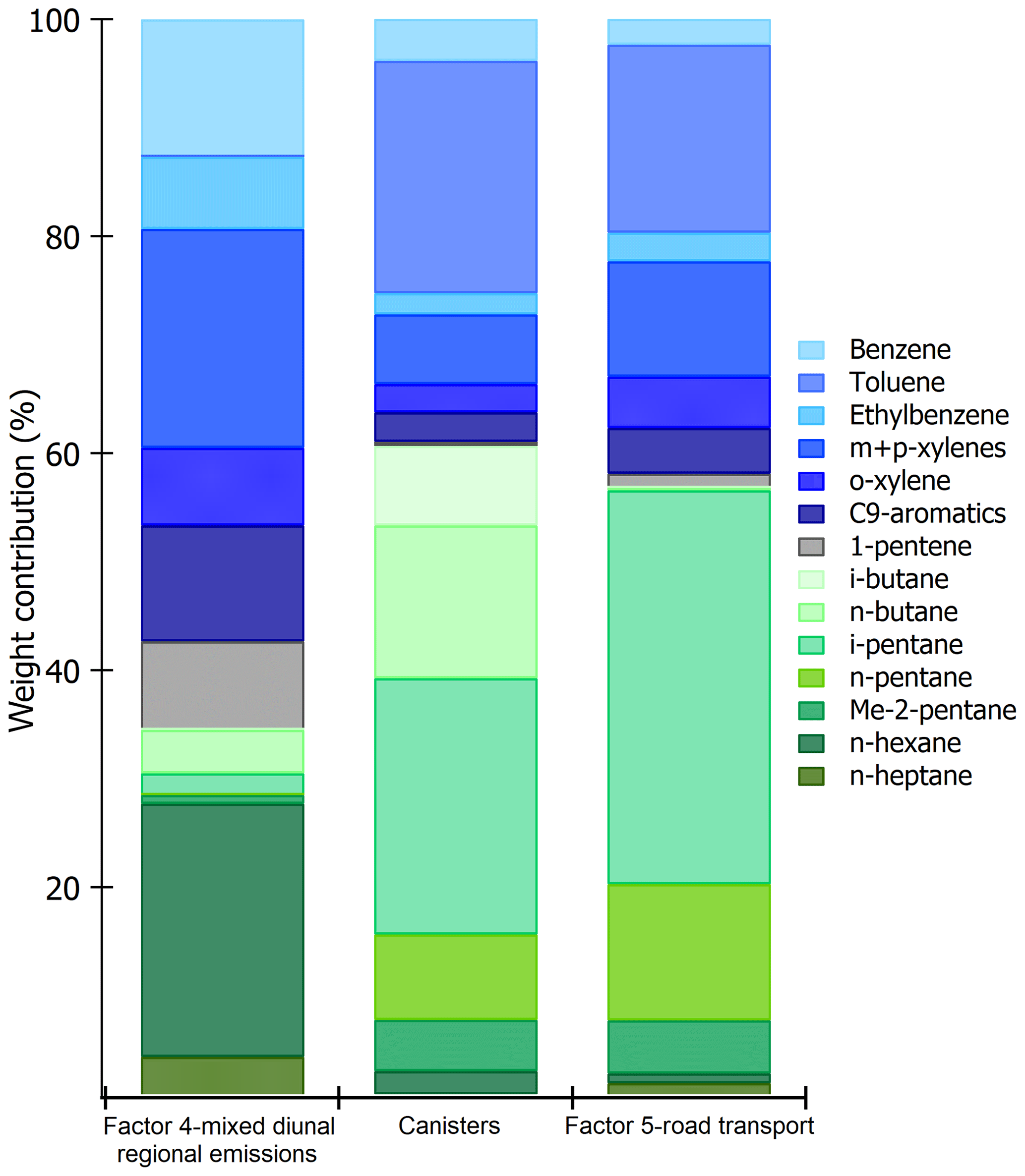
Figure 10Comparison of speciated profiles issued from canisters (traffic source) and factors 4 and 5 of PMF simulations. The species contributions are expressed in percentage volume.
Aromatic compounds (benzene 40 %, ethylbenzene 29 %, C9 aromatics 24 %, and xylenes 20 % on average) are also well represented in this factor. While they enter in the composition of fossil fuel combustion by constituting the unburned fraction of vehicle exhaust emissions as for C5 alkanes (Buzcu and Fraser, 2006), their proportion in factor 4 does not compare with that of traffic emissions derived from canister measurements along the Barbaros (Bd) (Fig. 10). Solvent use activities from domestic or industrial sectors can also emit aromatics higher than C6. Therefore, the presence of aromatics in factor 4 would be related to solvent use activities. Acetonitrile, highly present in factor 4, is usually used as a biomass burning tracer (Holzinger et al., 1999).
The diurnal profile is characterized by an increase in concentration during the day and a decrease in concentrations at night (Fig. 9). When looking at external variables, this factor correlates well with SO2 (R=0.5), which is a tracer of industrial emissions and ship emissions (Lee et al., 2011), but with neither NOx (R=0.25) nor CO (). Indeed the city of Istanbul experiences the highest industrial activities in the country (Markakis et al., 2012) while the Bosporus strait is 500 m away. The diurnal shape is also similar to that of ship traffic counts (Fig. S6 of the Supplement), which follows that of road traffic.
The potential influence of ship emissions has been investigated by looking at the ratio of V ∕ Ni derived from the elemental composition of PM2.5. This ratio has been commonly used as a tracer of ship emission influence (Viana et al., 2014; Pey et al., 2013; Becagli et al., 2012). While some papers assume that a ratio of 3 usually signifies the impact of ship emissions (Mazzei et al., 2008; Pandolfi et al., 2011), a deeper analysis of the literature suggests that this ratio is highly variable from 0.7 up to 4.5 (Isakson et al., 2001; Agrawal et al., 2008). When plotting particulate V versus Ni concentrations integrated over a 24 h period in September 2014, a ratio of 2.72±0.89 is found (see Fig. S7 in the Supplement). However, the scatterplot of 6 h integrated data reveals a more scattered distribution of points on both sides of the fitting line. First, the derived V-to-Ni value seems to be controlled by the sampling time resolution and a fixed value cannot be used as evidence of ship emission influence. Second, while the Istanbul points lie between the upper and lower limits, some of them are higher than 4.5. Other sources like coal combustion can affect the V and Ni distribution (Oztürk et al., 2019). Finally, by comparing this factor (C5–C7 alkanes, aromatic compounds, 1-pentene, and acetone) to that of ship emissions at berth in Jingtang port (Xiao et al., 2018), no similarity was found. While an influence of ship emissions is not excluded, there is no direct evidence from VOC measurements.
The analysis of the time series shows that the background level of this factor varies as a function of the meteorological period (Fig. 8). During period 2, an increase in minimum concentrations is observed, which may be related to the lower wind speed that favors the stagnation of pollutants. We assume that secondary production affects this factor since the presence of many secondary compounds (MACR + MVK, MEK, acetaldehyde, etc.) is observed. To conclude, this factor can be related to a combination of primary and secondary anthropogenic (combustion, industrial, and ship emissions) as well as biogenic emissions. By considering the different origins of species and their diurnal emission, this factor was labeled “mixed regional emissions factor”. It represents 36.3 % of the total VOC contribution.
By increasing the number of factors, isoprene was isolated into a seven-factor solution. By increasing the number of factors to eight, isoprene was not isolated anymore (Fig. S8). By using only the PTR-MS data (10 min time resolution) for the PMF run, isoprene and its oxidation products have been isolated as well. Synchronizing the PTR-MS data with the GC–FID time step (30 min resolution) degrades the time resolution and smooths the variability of the data and, consequently, the ability of the PMF model to isolate biogenic emissions from other sources.
Factor 5: Road transport
The profile of factor 5 exhibits high contributions of pentanes (iso, n, and 2-methyl) with on average 84 % of their variability explained by this factor (Fig. 7), followed by n-heptane (58 %). A total of 32 % of the variability of 1-pentene is also explained by this factor. Aromatic compounds, such as ethylbenzene (45 %), o-xylenes, (m + p)-xylenes (47 %), C9 aromatics (37 %), benzene (28 %), and toluene (28 %), which are considered typical fossil fuel combustion products (Sigsby et al., 1987), are also predominant species in this factor. Isopentane is one of the most abundant VOCs in the traffic-related sources (Buzcu and Fraser, 2006).
To help in identifying the main sources related to this factor, a comparison between its profile and that obtained from near-source traffic measurements was performed (see Fig. 10). Contrary to factor 4 (mixed regional emissions), both profiles are similar. Factor 5 is much more enriched in aromatics compared to C5 alkanes by almost a factor of 2.
The diurnal profile of factor 5 showed an increase in concentrations from midnight until sunrise and an almost constant concentration during the rest of the day with several small peaks (Fig. 9). Morning peaks (06:30 and 09:30) and a night peak (19:30) are observed. This increase in concentrations corresponds to the morning and evening traffic rush-hour periods. After 18:30 the absolute concentration of this factor stayed high and increased for several reasons: ongoing emissions until 3 h 30 min, lower photochemical reactions, and atmospheric dynamics (the shallower boundary layer leads to more accumulation of pollutants at night). Lower concentrations are observed during late morning until 18:30. The reduction of concentration of this factor during the day could be explained by dilution processes and OH oxidation processes.
The time series shows a period of a peak and a relatively high contribution of this factor in the night of 26 to 27 September (Fig. 8). Factor 5 is the closest to a traffic-related source that covers exhaust emissions and gasoline evaporation emissions. However, the contribution of this factor does not correlate with the traffic tracer NOx. This factor represents 15.8 % of the total VOC contribution.
As discussed in Yuan et al. (2012), the effect of photochemistry on factor composition had been analyzed by looking at the scatterplots of the contribution of the PMF factors to each VOC as a function of its OH rate constant (kOH). Nevertheless, no clear evidence from photochemistry was found for the Istanbul PMF factor's contributions.
This study shows that PMF was more easily able to extract some factors (like biogenic terpenes) than others (like diurnal regional factors). These results are consistent with other Turkish cities where sources other than traffic (mostly industrial source) drive the VOC emissions (Yurdakul et al., 2013b; Pekey and Hande, 2011; Civan et al., 2015; Dumanoglu et al., 2014). However, in the EMB, traffic-related emissions are the most dominant source and accounted for 51 % and 74 % in winter and summer, respectively, in Beirut, Lebanon (Salameh et al., 2016). Kaltsonoudis et al. (2016) also found that traffic and biogenic emissions were the dominant source of VOC during summer in Patras and Athens. In Paris, Baudic et al. (2016) found that 25 % of the total VOC contributions were related to traffic, 15 % to biogenic factors and 20 % to solvent use compared with 14.2 % and 23 % to natural gas and background factors that the PMF has not able to dissociate. These differences in contributions with this study could be due to the differences in input data. Thus, PMF results depend strongly on input data. Furthermore, it was shown in McDonald et al. (2018) that source apportionment studies largely underestimated the influence of volatile chemical species (including organic solvents, personal care products, adhesives, etc.) as sources of urban VOCs. This underestimation could be explained by the fact that VOCs are not measured in all their diversity in source apportionment studies in contrast with what was done in McDonald et al. (2018).
3.4 Emission ratios of VOC to CO
The determination of emission ratios (ERs) is a useful constraint to evaluate emission inventories (Warneke et al., 2007; Borbon et al., 2013). The emission ratio is the ratio of a selected VOC with a reference compound that does not undergo photochemical processing, mostly CO or acetylene due to their low reactivity at an urban scale and as tracers of incomplete combustion (Borbon et al., 2013; Salameh et al., 2017). The linear regression fit method (LRF) is a commonly used method to calculate emission ratios: the ER corresponds to the slope of the scatterplot between a given VOC and CO or acetylene (Borbon et al., 2013; Salameh et al., 2017). Another method is the photochemical age method (de Gouw et al., 2005, 2018; Warneke et al., 2007; Borbon et al., 2013), which is based on the concentration ratios and the photochemical age. In this study, poor correlation between targets VOC and CO is found (R2≤0.16) as could be deduced from the time series analysis (see Sect. 3.2.2) and the PMF analysis. Indeed, activities derived from fossil fuel combustion do not dominate the VOC distribution. As a consequence the LRF method cannot be applied. Here the emission ratio was determined by the mean value of each Δ(VOC)-to-Δ(CO) concentration ratio over the whole period of measurements. The terms “Δ(VOC)” and “Δ(CO)” correspond to the measured concentrations of VOC and CO subtracted by VOC and CO background concentrations, respectively. Given the diurnal and data day-to-day variability of dynamics (see Sect. 3.3.2), one daytime and one nighttime CO background value was estimated for each day by extracting the daytime and nighttime minimum concentration values. For CO, the daytime background values range between 213.5 and 367.2 ppb and the nighttime background values range between 211.5 and 406.7 ppb. For VOC, the background values depend on the compound. At night, the background values lie between 1.3 and 3.4 ppb for a long-lived compound like acetone and between 0.2 and 1.1 for a short-lived compound like the (m + p)-xylenes. For the following discussion, we will refer to the VOC-to-CO ratio instead of “Δ(VOC)-to-Δ(CO)” ratio.
Photochemistry can affect the value of emission ratios (Borbon et al., 2013). Comparing daytime to nighttime ratios is one way to evaluate the effect of daytime photochemistry by assuming that chemistry can be neglected at night except for alkenes (de Gouw et al., 2018), and the composition of emissions does not change between day and night. While the ratio between nighttime emission ratios and daytime emission ratios shows a decrease of 37 % on average during the day, this decrease is not dependent on the OH kinetic constants of each VOC (Fig. S9). This suggests that these differences are controlled by the changes in emission composition between day and night. As a consequence, the emission ratios have been determined for the whole dataset.
Table 3Urban VOC-to-CO emission ratios determined during the Istanbul field campaign and compared to the ones determined in Los Angeles (North America), Paris (Europe), Mexico (Central America), and Beirut (Middle East) during previous field campaigns. Bolded values are the ones within a range of a factor of ±2 between Istanbul and at least one other urban area.
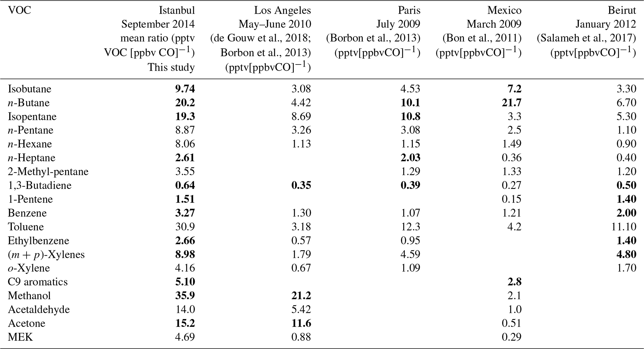
The emission ratios of VOCs to CO in Istanbul are displayed in Table 3 and compared to those in other urban areas worldwide. The emission ratios determined in Istanbul are usually higher than those of other cities but in the same range of magnitude. C4–C5 alkanes, toluene, and oxygenated VOCs show the highest emission ratio values. Most of the values are consistent within a factor of 2 with, at least, one determined in other cities of post-industrialized or developing countries.
3.5 Evaluation of global emission inventories
In this section, the VOC emissions from anthropogenic sources and road transport sources from three references global emission inventories downscaled to Istanbul are evaluated: MACCity (Granier et al., 2011) for 2014, EDGAR (Crippa et al., 2018) for 2012, and ACCMIP (Atmospheric Chemistry and Climate Model Intercomparison Project) (Lamarque et al., 2010) for 2000 (Fig. 11a, b, and c). Emission data for ACCMIP and MACCity inventories are available in the ECCAD database (http://eccad.aeris-data.fr/, last access: 16 July 2019), and the data for the EDGAR inventory are available in the EDGAR database (http://edgar.jrc.ec.europa.eu/, last access: 16 July 2019). This evaluation is based on the VOC-to-CO emission ratios calculated in the previous Sect. 3.4 following Salameh et al. (2016):
where
-
VOCestimated is the estimated emissions for an individual VOCs or a group of VOC in metric tons per year for all anthropogenic emissions or road transport emissions.
-
COinventory is the extracted emission of CO from ACCMIP (in teragrams per year), MACCity (in teragrams per year), or EDGAR (in metric tons per year).
-
VOC-to-CO ratio is either the VOC-to-CO ratio calculated in Sect. 3.4 or the VOC-to-CO ratio determined from each VOC contribution in the PMF road transport factor (in micrograms per cubic meter of VOC/micrograms per cubic meter of CO).
Species in emission inventories are sometimes lumped (grouped) as a function of their reactivity for chemical modeling purposes and species label does not always correspond to a single species. For instance, methanol in EDGAR not only corresponds to methanol itself but all alcohols. Moreover, summing some species from observations is sometimes needed to fit with the inventory lumping, like alkanes higher than C4 in MACCity, but is limited to the number of the measured species. As a consequence, the comparison is not direct and requires special care (see the following discussion).
The annual VOC and CO emissions for EDGAR (0.1×0.1 resolution) were determined by summing the emissions of 12 grids over a domain encompassing the sampling site (longitude between 28.9 and 29.1∘; latitude between 40.9 and 41.2∘). For ACCMIP and MACCity, the emission values for the city of Istanbul were taken as available in the ECCAD database.
Further information about the emission inventory can be found in Table S10 of the Supplement.
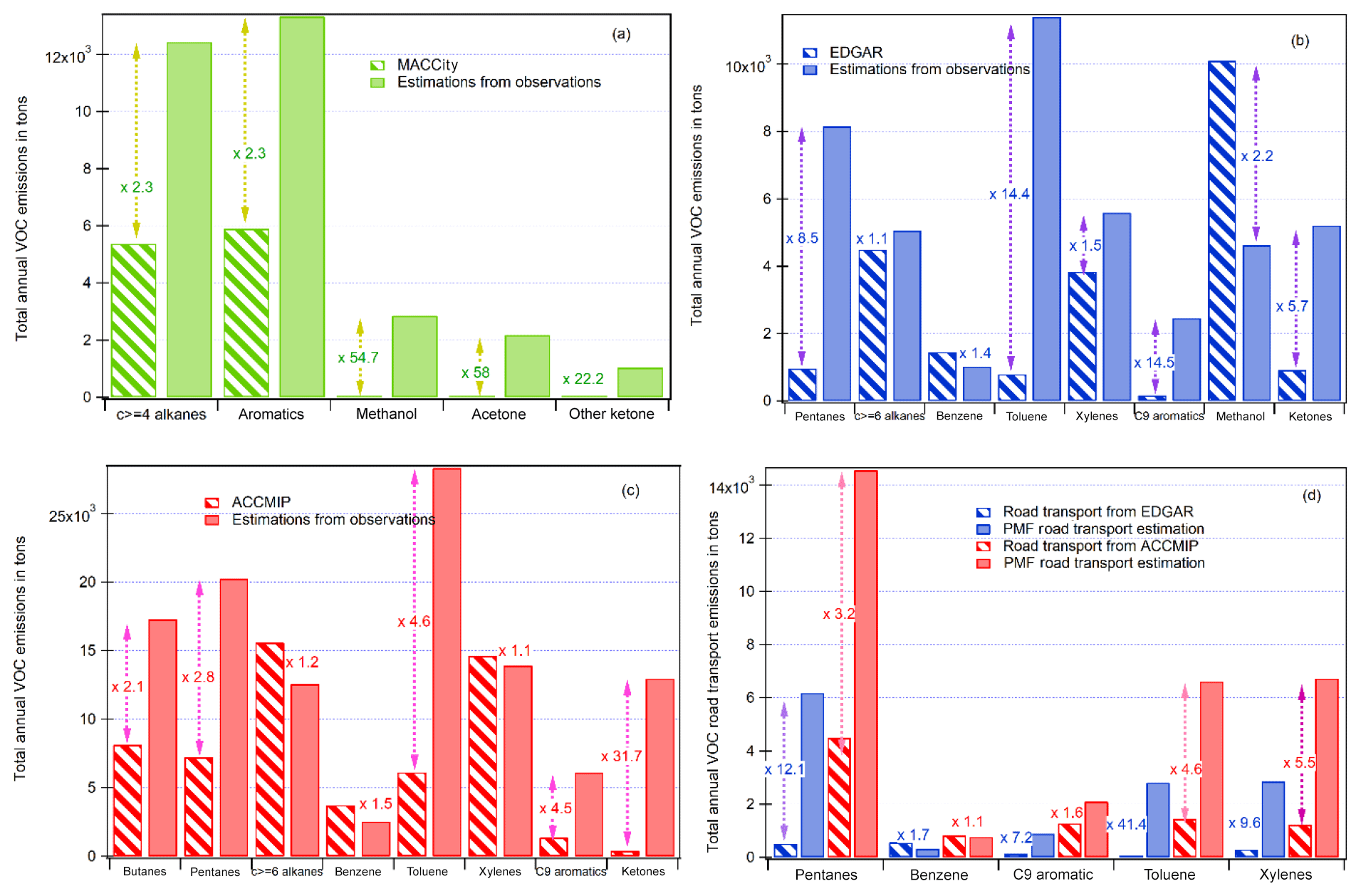
Figure 11Comparison of the estimated emission inventory from observations and PMF results and global emission inventories: (a) MACCity, (b) EDGAR, (c) ACCMIP, and (d) road transport from ACCMIP and EDGAR.
Figure 11 shows the comparison of the estimated emissions of some speciated VOCs derived from observations and PMF for the road transport and the ones from the three global emission inventories downscaled to the Istanbul megacity.
The total annual VOC anthropogenic emissions by global inventories are usually either within the same range by a factor of 2 to 3 for alkanes and aromatics or underestimated by an order of magnitude, especially for oxygenated compounds, up to a factor of 58 for acetone by EDGAR. These results are consistent with previous evaluations carried out in the Middle East (Salameh et al., 2016) and for northern midlatitude urban areas (Borbon et al., 2013). One exception is methanol in EDGAR, which is 2.2 times higher than our estimations from observations. This might be due to the inclusion of other alcohols in the methanol label in EDGAR as discussed above. One should note that the emissions of CO and VOCs from MACCity are usually lower than the ones from ACCMIP and EDGAR, which can be explained by the different year of reference. The global emissions by inventories were not within the same year: 2000 for ACCMIP, 2014 for MACCity, and 2012 for EDGAR. The CO emissions by inventories were compared for the same year. It was found that ACCMIP and MACCity had the same CO emissions while the emissions in Edgar were 2 times lower than those from MACCity and ACCMIP. In 2012, emissions of CO by EDGAR were similar to those of MACCity.
The evaluation of the road transport emissions (Fig. 11d) is limited to the compounds from the unburned fuel fraction; while there is still an underestimation by the emission inventories except for benzene, the differences are lower than for all anthropogenic emissions. The differences never exceed a factor of 12.1 (pentanes). Again, the differences for pentanes should be seen as a lower limit because of the number of measured pentanes, which are limited to n-pentane and isopentane.
While these results provide a first detailed evaluation of VOC annual emissions by global emission inventories, they are based on a limited period of observations in September 2014 (2 weeks). Additional VOC observations at different periods of the year including the heating and non-heating period will be very useful to strengthen this first evaluation by taking into account the seasonal variability of emissions. However, they confirm the urgent need in updating global emission inventories by taking into account region-specific emissions.
VOC measurements were performed in Istanbul (Turkey) at an urban site in Besiktas in September 2014. The VOC measurement instruments include an airmoVOC GC–FID and a PTR-MS at the super site completed with sorbent tubes and canisters within the megacity close to major emission sources. A total of 23 of the 70 NMHCs quantified were continuously collected at the urban site.
During the intense field campaign, three periods had been selected from the meteorological parameter analysis and limited by two transitional periods. VOC variabilities were driven by the meteorological conditions observed, with higher concentrations during period 2 (under continental influence) and lower concentrations during periods 1 and 3 (under marine influence). Also, most of the VOCs were characterized by an increase in concentrations at night and early morning and lower concentrations during the day.
The average composition of VOCs is mainly composed of OVOCs, which represent 43.9 % of the total VOC mixing ratio observed, followed by alkanes (26.33 %), aromatic compounds (20.66 %), alkenes (4.81 %), terpenes (3.44 %), and acetonitrile (0.84 %). The average atmospheric composition of anthropogenic VOCs is similar to those observed in European megacities like Paris and London, suggesting the impact of traffic emissions for those compounds. However, much evidence of the impact of sources other than traffic, like industrial activities under continental and south-southwesterly wind regimes or ship emissions on IVOC loads, has been found. This evidence was also observed in the time series analysis where the influence of multiple sources other than traffic was also suggested.
Time series and diurnal profile analyses suggest the influence of multiple sources other than traffic on VOC concentrations at the super site and likely industrial and/or port activities.
Five factors have been extracted by the model and then compared to source profiles established by off-line near-source measurements. These results also confirmed that road transport is not the dominant source by only explaining 15.8 % (factor 5) of measured VOC concentrations, differing from the local emission inventory. Other factors as sources resolved by the model were toluene (14.2 %), biogenic terpenes (7.8 %), natural gas evaporation (25.9 %, mainly composed of butanes), and a last factor characterized by mixed regional emissions (36.3 % and composed of most of the species). Evaluating the PMF results, there is no evidence of the impact of ship emissions on VOC distribution. It is also shown that the commonly used ship emission tracer derived from PM2.5 composition should be used with caution.
Several sensitivity tests on PMF results based on input data have been carried out to evaluate the effect of the time resolution when combining different instrumentation measurements. Sensitivity tests also analyzed the impacts due to the number of missing values and the number of species integrated in each model run as well as the impact of interpolation on input data. While some sensitivity tests do not perform as well as the reference run, they all showed that the same factors are identified even though their relative contributions could be slightly modified.
Considering our results and knowing that the measurement period was quite short, long-term measurements at different times of the year will be valuable to assess the seasonality effect on source contributions in Istanbul.
Emission ratios (ERs) of VOC relative to carbon monoxide (CO) were calculated and compared to those of many megacities. The emission ratios determined in Istanbul were found to usually be higher than those of other cities. These ERs have then been used to evaluate three global emission inventories: MACCity, ACCMIP, and EDGAR. The results showed that the total annual VOC anthropogenic emissions by global inventories are usually either within the same range by a factor of 2 to 3 for alkanes and aromatics or underestimated by an order of magnitude, especially for oxygenated compounds. For the road transport emissions, there is still an underestimation by global inventories except for benzene.
Even though these results provide a first detailed evaluation of VOC annual emissions by global emission inventories in Istanbul, measurements are carried out for a limited periods of time (2 weeks). Thus, longer measurement period at different seasons of the year will be very useful to strengthen and complete these results.
The data used for the study presented here can be provided upon request. Please contact Agnès Borbon (agnes.borbon@uca.fr).
The supplement related to this article is available online at: https://doi.org/10.5194/acp-19-15131-2019-supplement.
BTPT is a PhD student; she is responsible for the data analysis presented in this work. PD supported the data analysis. FÖ was the Turkish PI of the TRANSEMED Istanbul campaign. She dealt with the implementation of the super site and the aerosol measurements. TS supported the PMF output analysis. SS was one of the French partners of the project; he took part in the field campaign and supervised the analysis of VOC samples at the laboratory. CA was the Lebanese partner of the project; he took part in the field campaign for trace gas analysis and the scientific discussions. Banu Çetin is one of the Turkish partners; together with Fatma Ozturk she was in charge of the super site implementation and took part in the field campaign. CG was in charge of the trace gas measurements 675 (GC–FID, PTR-MS) on the field and chromatogram treatment, MK is a PhD student; she was in charge of the PM measurements in the field and their analysis at the laboratory. SE implemented the FLEXPART model, and AB is the PI of the TRANSEMED project. She coordinates the project and supervises BTPT's PhD.
The authors declare that they have no conflict of interest.
CHemistry and AeRosols Mediterranean EXperiments (ChArMEx) (ACP/AMT inter-journal SI) SI statement: This article is part of the special issue “CHemistry and AeRosols Mediterranean EXperiments (ChArMEx) (ACP/AMT inter-journal SI)”. It is not associated with a conference.
The French and Turkish ChArMEx/MISTRAL and TÜBİTAK, respectively, are acknowledged here. The grant provided by Bolu Abant Izzet Baysal University (BAIBU) Scientific Research Projects Coordination Office (BAP) is also acknowledged (grant number 2015.09.02.825).
The field campaign in Istanbul was supported by the ENVIMED/MISTRALS 2013 call. This work is also part of the ChArMEx program. ChArMEx is the atmospheric component of the French multidisciplinary program MISTRALS (Mediterranean Integrated Studies at Regional and Local Scales). ChArMEx France was principally funded by INSU, ADEME, ANR, CNES, CTC (Corsica region), EU/FEDER, Météo-France, and CEA. This study is also partly supported by the Scientific and Technological Research Council of Turkey (TUBITAK) with the project number 113Y025. This research has been supported by ENVIMED the Bolu Abant Izzet Baysal University Scientific Research Projects Coordination Office (grant no. 2015.09.02.825).
This paper was edited by Evangelos Gerasopoulos and reviewed by two anonymous referees.
Agrawal, H., Malloy, Q. G. J., Welch, W. A., Wayne Miller, J., and Cocker, D. R.: In-use gaseous and particulate matter emissions from a modern ocean going container vessel, Atmos. Environ., 42, 5504–5510, https://doi.org/10.1016/j.atmosenv.2008.02.053, 2008.
Ait-Helal, W., Borbon, A., Sauvage, S., de Gouw, J. A., Colomb, A., Gros, V., Freutel, F., Crippa, M., Afif, C., Baltensperger, U., Beekmann, M., Doussin, J.-F., Durand-Jolibois, R., Fronval, I., Grand, N., Leonardis, T., Lopez, M., Michoud, V., Miet, K., Perrier, S., Prévôt, A. S. H., Schneider, J., Siour, G., Zapf, P., and Locoge, N.: Volatile and intermediate volatility organic compounds in suburban Paris: variability, origin and importance for SOA formation, Atmos. Chem. Phys., 14, 10439–10464, https://doi.org/10.5194/acp-14-10439-2014, 2014.
Atkinson, R.: Atmospheric chemistry of VOCs and NOx, Atmos. Environ., 34, 2063–2101, https://doi.org/10.1016/S1352-2310(99)00460-4, 2000.
Batterman, S., Hatzivasilis, G., and Jia, C.: Concentrations and emissions of gasoline and other vapors from residential vehicle garages, Atmos. Environ., 40, 1828–1844, 2006.
Batterman, S., Su, F. C., Li, S., Mukherjee, B., and Jia, C.: Personal exposure to mixtures of volatile organic compounds: modeling and further analysis of the RIOPA Data, Res. Rep. Health Eff. Inst., 181, 3–63, 2014.
Baudic, A., Gros, V., Sauvage, S., Locoge, N., Sanchez, O., Sarda-Estève, R., Kalogridis, C., Petit, J.-E., Bonnaire, N., Baisnée, D., Favez, O., Albinet, A., Sciare, J., and Bonsang, B.: Seasonal variability and source apportionment of volatile organic compounds (VOCs) in the Paris megacity (France), Atmos. Chem. Phys., 16, 11961–11989, https://doi.org/10.5194/acp-16-11961-2016, 2016.
Becagli, S., Sferlazzo, D. M., Pace, G., di Sarra, A., Bommarito, C., Calzolai, G., Ghedini, C., Lucarelli, F., Meloni, D., Monteleone, F., Severi, M., Traversi, R., and Udisti, R.: Evidence for heavy fuel oil combustion aerosols from chemical analyses at the island of Lampedusa: a possible large role of ships emissions in the Mediterranean, Atmos. Chem. Phys., 12, 3479–3492, https://doi.org/10.5194/acp-12-3479-2012, 2012.
Bon, D. M., Ulbrich, I. M., de Gouw, J. A., Warneke, C., Kuster, W. C., Alexander, M. L., Baker, A., Beyersdorf, A. J., Blake, D., Fall, R., Jimenez, J. L., Herndon, S. C., Huey, L. G., Knighton, W. B., Ortega, J., Springston, S., and Vargas, O.: Measurements of volatile organic compounds at a suburban ground site (T1) in Mexico City during the MILAGRO 2006 campaign: measurement comparison, emission ratios, and source attribution, Atmos. Chem. Phys., 11, 2399–2421, https://doi.org/10.5194/acp-11-2399-2011, 2011.
Borbon, A., Locoge, N., Veillerot, M., Galloo, J. C., and Guillermo, R.: Characterisation of NMHCs in a French urban atmosphere: Overview of the main sources, Sci. Total. Environ., 292, 177–191, https://doi.org/10.1016/S0048-9697(01)01106-8, 2002.
Borbon, A., Gilman, J. B., Kuster, W. C., Grand, N., Chevaillier, S., Colomb, A., Dolgorouky, C., Gros, V., Lopez, M., Sarda-Esteve, R., Holloway, J., Stutz, J., Petetin, H., McKeen, S., Beekmann, M., Warneke, C., Parrish, D. D., and de Gouw, J. A.: Emission ratios of anthropogenic volatile organic compounds in northern mid-latitude megacities: Observations versus emission inventories in Los Angeles and Paris, J. Geophys. Res.-Atmos., 118, 2041–2057, https://doi.org/10.1002/jgrd.50059, 2013.
Borbon, A., Boynard, A., Salameh, T., Baudic, A., Gros, V., Gauduin, J., Perrussel, O., and Pallares, C.: Is Traffic Still an Important Emitter of Monoaromatic Organic Compounds in European Urban Areas?, Environ. Sci. Technol., 52, 513–521, https://doi.org/10.1021/acs.est.7b01408, 2018.
Bozkurt, Z., Özden, Ö., Dö, T., Artun, G., and Gaga, E. O.: Atmospheric concentrations of SO2, NO2 , ozone and VOCs in Düzce, Turkey using passive air samplers?: Sources, spatial and seasonal variations and health risk estimation, Atmos. Pollut. Res., 1146–1156, https://doi.org/10.1016/j.apr.2018.05.001, 2018.
Brioude, J., Arnold, D., Stohl, A., Cassiani, M., Morton, D., Seibert, P., Angevine, W., Evan, S., Dingwell, A., Fast, J. D., Easter, R. C., Pisso, I., Burkhart, J., and Wotawa, G.: The Lagrangian particle dispersion model FLEXPART-WRF version 3.1, Geosci. Model Dev., 6, 1889–1904, https://doi.org/10.5194/gmd-6-1889-2013, 2013.
Brocco, D., Fratarcangeli, R., Lepore, L., Petricca, M., and Ventrone, I.: Determination of aromatic hydrocarbons in urban air of Rome, Atmos. Environ., 31, 557–566, https://doi.org/10.1016/S1352-2310(96)00226-9, 1997.
Brown, S. G., Frankel, A., and Hafner, H. R.: Source apportionment of VOCs in the Los Angeles area using positive matrix factorization, Atmos. Environ., 41, 227–237, https://doi.org/10.1016/J.ATMOSENV.2006.08.021, 2007.
Buzcu, B. and Fraser, M. P.: Source identification and apportionment of volatile organic compounds in Houston, TX, Atmos. Environ., 40, 2385–2400, https://doi.org/10.1016/j.atmosenv.2005.12.020, 2006.
Civan, M. Y., Elbir, T., Seyfioglu, R., Kuntasal, Ö. O., Bayram, A., Dogan, G., Yurdakul, S., Andiç, O., Müezzinoglu, A., Sofuoglu, S. C., Pekey, H., Pekey, B., Bozlaker, A., Odabasi, M., and Tuncel, G.: Spatial and temporal variations in atmospheric VOCs, NO2, SO2, and O3 concentrations at a heavily industrialized region in Western Turkey, and assessment of the carcinogenic risk levels of benzene, Atmos. Environ., 103, 102–113, https://doi.org/10.1016/j.atmosenv.2014.12.031, 2015.
Crippa, M., Guizzardi, D., Muntean, M., Schaaf, E., Dentener, F., van Aardenne, J. A., Monni, S., Doering, U., Olivier, J. G. J., Pagliari, V., and Janssens-Maenhout, G.: Gridded emissions of air pollutants for the period 1970–2012 within EDGAR v4.3.2, Earth Syst. Sci. Data, 10, 1987–2013, https://doi.org/10.5194/essd-10-1987-2018, 2018.
de Gouw, J. A., Middlebrook, A. M., Warneke, C., Goldan, P. D., Kuster, W. C., Roberts, J. M., Fehsenfeld, F. C., Worsnop, D. R., Canagaratna, M. R., Pszenny, A. A. P., Keene, W. C., Marchewka, M., Bertman, S. B., and Bates, T. S.: Budget of organic carbon in a polluted atmosphere: Results from the New England Air Quality Study in 2002, J. Geophys. Res., 110, D16305, https://doi.org/10.1029/2004JD005623, 2005.
de Gouw, J. A., Gilman, J. B., Kim, S. W., Lerner, B. M., Isaacman-Van Wertz, G., McDonald, B. C., Alvarez, S. L., Dusanter, S., Stutz, J., Graus, M., Griffith, S. M., Kuster, W. C., Lefer, B. L., Rappenglück, B., Roberts, J. M., Stevens, P. S., Thalman, R., Veres, P. R., Volkamer, R., Warneke, C., Washenfelder, R. A., and Young, C. J.: Chemistry of Volatile Organic Compounds in the Los Angeles Basin: Formation of Oxygenated Compounds and Determination of Emission Ratios, J. Geophys. Res.-Atmos., 123, 2298–2319, https://doi.org/10.1002/2017JD027976, 2018.
Debevec, C., Sauvage, S., Gros, V., Sciare, J., Pikridas, M., Stavroulas, I., Salameh, T., Leonardis, T., Gaudion, V., Depelchin, L., Fronval, I., Sarda-Esteve, R., Baisnée, D., Bonsang, B., Savvides, C., Vrekoussis, M., and Locoge, N.: Origin and variability in volatile organic compounds observed at an Eastern Mediterranean background site (Cyprus), Atmos. Chem. Phys., 17, 11355–11388, https://doi.org/10.5194/acp-17-11355-2017, 2017.
Demir, S., Saral, A., Išik, D., Akyildiz, A., Levent Kuzu, S., Mert, S., Demir, G., and Goncaloglu, B. I.: Characterization of ambient volatile organic compounds and their diurnal variations in Istanbul, Turkey, Fresen. Environ. Bull., 20, 2951–2958, 2011.
Detournay, A., Sauvage, S., Locoge, N., Gaudion, V., Leonardis, T., Fronval, I., Kaluzny, P., and Galloo, J.-C.: Development of a sampling method for the simultaneous monitoring of straight-chain alkanes, straight-chain saturated carbonyl compounds and monoterpenes in remote areas, J. Environ. Monit., 13, 983–990, https://doi.org/10.1039/c0em00354a, 2011.
Dominutti, P. A., Nogueira, T., Borbon, A., Andrade, M. de F., and Fornaro, A.: One-year of NMHCs hourly observations in São Paulo megacity: meteorological and traffic emissions effects in a large ethanol burning context, Atmos. Environ., 142, 371–382, https://doi.org/10.1016/j.atmosenv.2016.08.008, 2016.
Dumanoglu, Y., Kara, M., Altiok, H., Odabasi, M., Elbir, T., and Bayram, A.: Spatial and seasonal variation and source apportionment of volatile organic compounds (VOCs) in a heavily industrialized region, Atmos. Environ., 98, 168–178, https://doi.org/10.1016/J.ATMOSENV.2014.08.048, 2014.
Elbir, T., Cetin, B., Cetin, E., Bayram, A., and Odabasi, M.: Characterization of Volatile Organic Compounds (VOCs) and Their Sources in the Air of Izmir, Turkey, Environ. Monit. Assess., 133, 149–160, https://doi.org/10.1007/s10661-006-9568-z, 2007.
Ferm, M., De Santis, F., and Varotsos, C.: Nitric acid measurements in connection with corrosion studies, Atmos. Environ., 39, 6664–6672, https://doi.org/10.1016/J.ATMOSENV.2005.07.044, 2005.
Filella, I. and Peñuelas, J.: Daily, weekly, and seasonal time courses of VOC concentrations in a semi-urban area near Barcelona, Atmos. Environ., 40, 7752–7769, https://doi.org/10.1016/j.atmosenv.2006.08.002, 2006.
Finlayson-Pitts, B. J. and Pitts, J. N.: Chemistry of the Upper and Lower Atmosphere Theory, Experiments, and Applications, available at: http://www.sciencedirect.com/science/book/9780122570605 (last access: December 2017), Academic Press, San Diego, California, 2000.
Fuentes, J. D., Lerdau, M., Atkinson, R., Baldocchi, D., Bottenheim, J. W., Ciccioli, P., Lamb, B., Geron, C., Gu, L., Guenther, A., Sharkey, T. D., and Stockwell, W.: Biogenic Hydrocarbons in the Atmospheric Boundary Layer: A Review, B. Am. Meteor. Soc., 81, 1537–1575, https://doi.org/10.1175/1520-0477(2000)081<1537:BHITAB>2.3.CO;2, 2000.
Fuzzi, S., Andreae, M. O., Huebert, B. J., Kulmala, M., Bond, T. C., Boy, M., Doherty, S. J., Guenther, A., Kanakidou, M., Kawamura, K., Kerminen, V.-M., Lohmann, U., Russell, L. M., and Pöschl, U.: Critical assessment of the current state of scientific knowledge, terminology, and research needs concerning the role of organic aerosols in the atmosphere, climate, and global change, Atmos. Chem. Phys., 6, 2017–2038, https://doi.org/10.5194/acp-6-2017-2006, 2006.
Gaimoz, C., Sauvage, S., Gros, V., Herrmann, F., Williams, J., Locoge, N., Perrusel, O., Bonsang, B., d'Argouges, O., Sarda-Estève, R., and Sciare, J.: Volatile organic compounds sources in Paris in spring 2007, Part II: source apportionment using positive matrix factorization, Environ. Chem., 8, 91–103, https://doi.org/10.1071/EN10067, 2011.
Gelencsér, A., Siszler, K., and Hlavay, J.: Toluene-benzene concentration ratio as a tool for characterizing the distance from vehicular emission sources, Environ. Sci. Technol., 31, 2869–2872. https://doi.org/10.1021/es970004c, 1997.
Geron, C., Guenther, A., Sharkey, T., and Arnts, R. R.: Temporal variability in basal isoprene emission factor, Tree Physiol., 20, 799–805, https://doi.org/10.1093/treephys/20.12.799, 2000.
Goldstein, A. and Galbally, I.: Known and unexplored organic constituents in the earth's atmosphere, 1514–1527, available at: http://pubs.acs.org/doi/pdf/10.1021/es072476p (last access: 11 May 2018), 2007.
Goldstein, A. H. and Schade, G. W.: Quantifying biogenic and anthropogenic contributions to acetone mixing ratios in a rural environment, Atmos. Environ., 34, 4997–5006, https://doi.org/10.1016/S1352-2310(00)00321-6, 2000.
Goldstein, A. H., Fan, S. M., Goulden, M. L., Munger, J. W., and Wofsy, S. C: Emissions of ethene, propene, and 1 -butene by a midlatitude forest, J. Geophys. Res.-Atmos., 101, 9149–9157, https://doi.org/10.1029/96JD00334, 1996.
Granier, C., Bessagnet, B., Bond, T., D'Angiola, A., Denier van der Gon, H., Frost, G. J., Heil, A., Kaiser, J. W., Kinne, S., Klimont, Z., Kloster, S., Lamarque, J.-F., Liousse, C., Masui, T., Meleux, F., Mieville, A., Ohara, T., Raut, J.-C., Riahi, K., Schultz, M. G., Smith, S. J., Thompson, A., Aardenne, J. V., van der Werf, G. R., and van Vuuren, D. P.: Evolution of anthropogenic and biomass burning emissions of air pollutants at global and regional scales during the 1980–2010 period, Clim. Change, 109, 163–190, https://doi.org/10.1007/s10584-011-0154-1, 2011.
Grice, S., Stedman, J., Kent, A., Hobson, M., Norris, J., Abbott, J., and Cooke, S.: Recent trends and projections of primary NO2 emissions in Europe, Atmos. Environ., 43, 2154–2167, https://doi.org/10.1016/j.atmosenv.2009.01.019, 2009.
Harrison, D., Hunter, M., Lewis, A., Seakins, P., Nunes, T., and Pio, C.: Isoprene and monoterpene emission from the coniferous species Abies Borisii-regis – implications for regional air chemistry in Greece, Atmos. Environ., 35, 4687–4698, https://doi.org/10.1016/S1352-2310(01)00092-9, 2001.
Heeb, N., Forss, A., Bach, C., Reimann, S., Herzog, A., and Jäckle, H.: A comparison of benzene, toluene and C2-benzenes mixing ratios in automotive exhaust and in the suburban atmosphere during the introduction of catalytic, Atmos. Environ., 34, 3103–3116, https://doi.org/10.1016/S1352-2310(99)00446-X, 2000.
Hester, R. E. and Harrison, R. M. (Eds.): Volatile organic compounds in the atmosphere, Royal Society of Chemistry, Cambridge, 1995.
Hoerger, C. C., Claude, A., Plass-Duelmer, C., Reimann, S., Eckart, E., Steinbrecher, R., Aalto, J., Arduini, J., Bonnaire, N., Cape, J. N., Colomb, A., Connolly, R., Diskova, J., Dumitrean, P., Ehlers, C., Gros, V., Hakola, H., Hill, M., Hopkins, J. R., Jäger, J., Junek, R., Kajos, M. K., Klemp, D., Leuchner, M., Lewis, A. C., Locoge, N., Maione, M., Martin, D., Michl, K., Nemitz, E., O’Doherty, S., Pérez Ballesta, P., Ruuskanen, T. M., Sauvage, S., Schmidbauer, N., Spain, T. G., Straube, E., Vana, M., Vollmer, M. K., Wegener, R., and Wenger, A.: ACTRIS non-methane hydrocarbon intercomparison experiment in Europe to support WMO GAW and EMEP observation networks, Atmos. Meas. Tech., 8, 2715–2736, https://doi.org/10.5194/amt-8-2715-2015, 2015.
Holzinger, R., Wameke, C., Hansel, A., Jordan, A., Lindinger, W., Scharffe, D. H., Schade, G., and Crutzen, P. J.: Biomass burning as a source of formaldehyde, acetaldehyde, methanol, acetone, acetonitrile, and hydrogen cyanide, Geophys. Res. Lett., 26, 1161–1164, https://doi.org/10.1029/1999GL900156, 1999.
Huang, Y. S. and Hsieh, C. C.: Ambient volatile organic compound presence in the highly urbanized city: source apportionment and emission position, Atmos. Environ., 206, 45–59, https://doi.org/10.1016/J.ATMOSENV.2019.02.046, 2019.
İm, U., Tayanç, M., and Yenigün, O.: Interaction patterns of major photochemical pollutants in Istanbul, Turkey, Atmos. Res., 89, 382–390, https://doi.org/10.1016/J.ATMOSRES.2008.03.015, 2008.
Isakson, J., Persson, T. A., and Selin Lindgren, E.: Identification and assessment of ship emissions and their effects in the harbour of Göteborg, Sweden, Atmos. Environ., 35, 3659–3666, https://doi.org/10.1016/S1352-2310(00)00528-8, 2001.
Kalabokas, P., Bartzis, J. G., Bomboi, T., Ciccioli, P., Cieslik, S., Dlugi, R., Foster, P., Kotzias, D., and Steinbrecher, R.: Ambient atmospheric trace gas concentrations and meteorological parameters during the first BEMA measuring campaign on May 1994 at Castelporziano, Italy, Atmos. Environ., 31, 67–77, https://doi.org/10.1016/S1352-2310(97)00075-7, 1997.
Kaltsonoudis, C., Kostenidou, E., Florou, K., Psichoudaki, M., and Pandis, S. N.: Temporal variability and sources of VOCs in urban areas of the eastern Mediterranean, Atmos. Chem. Phys., 16, 14825–14842, https://doi.org/10.5194/acp-16-14825-2016, 2016.
Kesselmeier, J. and Staudt, M.: Biogenic Volatile Organic Compounds (VOC): An Overview on Emission, Physiology and Ecology, J. Atmos. Chem., 33, 23–88, https://doi.org/10.1023/A:1006127516791, 1999.
Keuken, M. P., Roemer, M. G. M., Zandveld, P., Verbeek, R. P., and Velders, G. J. M.: Trends in primary NO2 and exhaust PM emissions from road traffic for the period 2000–2020 and implications for air quality and health in the Netherlands, Atmos. Environ., 54, 313–319, https://doi.org/10.1016/J.ATMOSENV.2012.02.009, 2012.
Koçak, M., Theodosi, C., Zarmpas, P., Im, U., Bougiatioti, A., Yenigun, O., and Mihalopoulos, N.: Particulate matter (PM10) in Istanbul: Origin, source areas and potential impact on surrounding regions, Atmos. Environ., 45, 6891–6900, https://doi.org/10.1016/j.atmosenv.2010.10.007, 2011.
Koppmann, R. (Ed.).: Volatile organic compounds in the atmosphere, Blackwell Pub., Oxford, 2007.
Kousoulidou, M., Ntziachristos, L., Mellios, G., and Samaras, Z.: Road-transport emission projections to 2020 in European urban environments, Atmos. Environ., 42, 7465–7475, https://doi.org/10.1016/j.atmosenv.2008.06.002, 2008.
Kuntasal, Ö. O., Kılavuz, S. A., Karman, D., Wang, D., and Tuncel, G.: C5–C12 volatile organic compounds at roadside, residential, and background locations in Ankara, Turkey: Temporal and spatial variations and sources, J. Air. Waste. Manage. Assoc., 63, 1148–1162, https://doi.org/10.1080/10962247.2013.804012, 2013.
Lamarque, J.-F., Bond, T. C., Eyring, V., Granier, C., Heil, A., Klimont, Z., Lee, D., Liousse, C., Mieville, A., Owen, B., Schultz, M. G., Shindell, D., Smith, S. J., Stehfest, E., Van Aardenne, J., Cooper, O. R., Kainuma, M., Mahowald, N., McConnell, J. R., Naik, V., Riahi, K., and van Vuuren, D. P.: Historical (1850–2000) gridded anthropogenic and biomass burning emissions of reactive gases and aerosols: methodology and application, Atmos. Chem. Phys., 10, 7017–7039, https://doi.org/10.5194/acp-10-7017-2010, 2010.
Lanz, V. A., Hueglin, C., Buchmann, B., Hill, M., Locher, R., Staehelin, J., and Reimann, S.: Receptor modeling of C2–C7 hydrocarbon sources at an urban background site in Zurich, Switzerland: changes between 1993–1994 and 2005–2006, Atmos. Chem. Phys., 8, 2313–2332, https://doi.org/10.5194/acp-8-2313-2008, 2008.
Lee, C., Martin, R. V., van Donkelaar, A., Lee, H., Dickerson, R. R., Hains, J. C., Krotkov, N., Richter, A., Vinnikov, A., and Schwab, J. J.: SO2 emissions and lifetimes: Estimates from inverse modeling using in situ and global, space-based (SCIAMACHY and OMI) observations, J. Geophys. Res., 116, D06304, https://doi.org/10.1029/2010JD014758, 2011.
Lee, E., Chan, C. K., and Paatero, P.: Application of positive matrix factorization in source apportionment of particulate pollutants in Hong Kong, Atmos. Environ., 33, 3201–3212, https://doi.org/10.1016/S1352-2310(99)00113-2, 1999.
Lee, S. C., Chiu, M. Y., Ho, K. F., Zou, S. C., and Wang, X.: Volatile organic compounds (VOCs) in urban atmosphere of Hong Kong, Chemosphere, 48, 375–382, https://doi.org/10.1016/S0045-6535(02)00040-1, 2002.
Lelieveld, J., Hadjinicolaou, P., Kostopoulou, E., Chenoweth, J., El Maayar, M., Giannakopoulos, C., Hannides, C., Lange, M. A., Tanarhte, M., Tyrlis, E., and Xoplaki, E.: Climate change and impacts in the Eastern Mediterranean and the Middle East, Clim. Change, 114, 667–687, https://doi.org/10.1007/s10584-012-0418-4, 2012.
Liao, H. T., Yau, Y. C., Huang, C. S., Chen, N., Chow, J. C., Watson, J. G., Tsai, S. W., Chou, C. C. K., and Wu, C. F.: Source apportionment of urban air pollutants using constrained receptor models with a priori profile information, Environ. Pollut., 227, 323–333, https://doi.org/10.1016/J.ENVPOL.2017.04.071, 2017.
Macdonald, R. C. and Fall, R.: Acetone emission from conifer buds, Phytochemistry, 34, 991–994, https://doi.org/10.1016/S0031-9422(00)90700-3, 1993.
Markakis, K., Im, U., Unal, A., Melas, D., Yenigun, O., and Incecik, S.: Compilation of a GIS based high spatially and temporally resolved emission inventory for the greater Istanbul area, Atmos. Pollut. Res., 3, 112–125. https://doi.org/10.5094/APR.2012.011, 2012.
Matson, P., Lohse, K. A., and Hall, S. J.: The Globalization of Nitrogen Deposition: Consequences for Terrestrial Ecosystems, AMBIO, J. Hum. Environ. Syst., 31, 113–119, https://doi.org/10.1579/0044-7447-31.2.113, 2002.
Mazzei, F., D'Alessandro, A., Lucarelli, F., Nava, S., Prati, P., Valli, G., and Vecchi, R.: Characterization of particulate matter sources in an urban environment, Sci. Total. Environ., 401, 81–89, https://doi.org/10.1016/j.scitotenv.2008.03.008, 2008.
McDonald, B. C., de Gouw, J. A., Gilman, J. B., Jathar, S. H., Akherati, A., Cappa, C. D., Jimenez, J. L., Julia, L.-T., Hayes, P. L., McKeen, S. A., Cui, Y. Y., Kim, S.-W., Gentner, D. R., Isaacman-Van Wertz, G., Goldstein, A. H., Harley, R. A., Frost, G. J., Roberts, J. M., Ryerson, T. B., and Trainer, M.: Volatile chemical products emerging as largest petrochemical source of urban organic emissions, Science, 764, 760–764, https://doi.org/10.1126/science.aaq0524, 2018.
Millet, D. B., Guenther, A., Siegel, D. A., Nelson, N. B., Singh, H. B., de Gouw, J. A., Warneke, C., Williams, J., Eerdekens, G., Sinha, V., Karl, T., Flocke, F., Apel, E., Riemer, D. D., Palmer, P. I., and Barkley, M.: Global atmospheric budget of acetaldehyde: 3-D model analysis and constraints from in-situ and satellite observations, Atmos. Chem. Phys., 10, 3405–3425, https://doi.org/10.5194/acp-10-3405-2010, 2010.
Muezzinoglu, A., Odabasi, M., and Onat, L.: Volatile organic compounds in the air of Izmir, Turkey, Atmos. Environ., 35, 753–760, https://doi.org/10.1016/S1352-2310(00)00420-9, 2001.
Müller, J.-F.: Geographical distribution and seasonal variation of surface emissions and deposition velocities of atmospheric trace gases, J. Geophys. Res., 97, 3787, https://doi.org/10.1029/91JD02757, 1992.
Na, G., Kim, Y., and Kim, Y.: Concentrations of C2-C9 Volatile Organic Compounds in Ambient Air in Seoul, J. Korean Soc. Atmos. Environ., 14, 95–106, 1998.
Na, K. and Kim, Y. P.: Seasonal characteristics of ambient volatile organic compounds in Seoul, Korea, Atmos. Environ., 35, 2603–2614, https://doi.org/10.1016/S1352-2310(00)00464-7, 2001.
Nel, A.: Atmosphere, Air pollution-related illness: effects of particles, Science, 308, 804–806, https://doi.org/10.1126/science.1108752, 2005.
Norris, G., Duvall, R., Brown, S., and Bai, S.: EPA Positive Matrix Factorization (PMF) 5.0: Fundamentals & User Guide, Prepared for the US, Environmental Protection Agency (EPA), Washington, DC, by the National Exposure Research Laboratory, Research Triangle Park; Sonoma Technology, Inc., Petaluma, 2014.
OpenStreetMap contributors: Maps of Istanbul city, Marmara region, available at: https://www.openstreetmap.org/#map=7/51.330/10.453 (last access: 3 July 2019), 2015.
Owen, S., Boissard, C., Street, R. A., Duckham, S. C., Csiky, O., and Hewitt, C. N.: Screening of 18 Mediterranean plant species for volatile organic compound emissions, Atmos. Environ., 31, 101–117, https://doi.org/10.1016/S1352-2310(97)00078-2, 1997.
Öztürk, F., Melek Keleş, M., Çetin, B., Afif, C., Borbon, A., Yurdakul, S., Sauvage, S., Mihalopoulos, N., Zarmpas, P., Szidat, S., and Ünal, A.: Source Apportionment of Aerosols over Mega-city İstanbul: Findings from TRANSEMED Field Campaign, in preparation, 2019.
Paatero, P. and Tapper, U.: Positive MAtrix Factorization: a non- negative factor model with optimal utilization of error estimates of data values, Environmetrics, 5, 111–126, 1994.
Paatero, P. and Hopke, P. K.: Discarding or downweighting high-noise variables in factor analytic models, Anal. Chim. Acta, 490, 277–289, https://doi.org/10.1016/S0003-2670(02)01643-4, 2003.
Paatero, P., Eberly, S., Brown, S. G., and Norris, G. A.: Methods for estimating uncertainty in factor analytic solutions, Atmos. Meas. Tech., 7, 781–797, https://doi.org/10.5194/amt-7-781-2014, 2014.
Pandolfi, M., Gonzalez-Castanedo, Y., Alastuey, A., de la Rosa, J. D., Mantilla, E., de la Campa, A. S., Querol, X., Pey, J., Amato, F., Moreno, T.: Source apportionment of PM10 and PM2.5 at multiple sites in the strait of Gibraltar by PMF: impact of shipping emissions, Environ. Sci. Pollut. Res., 18, 260–269, https://doi.org/10.1007/s11356-010-0373-4, 2011.
Pekey, B. and Hande, Y.: The use of passive sampling to monitor spatial trends of volatile organic compounds (VOCs) at an industrial city of Turkey, Microchem. J., 97, 213–219, https://doi.org/10.1016/j.microc.2010.09.006, 2011.
Pey, J., Pérez, N., Cortés, J., Alastuey, A., and Querol, X.: Chemical fingerprint and impact of shipping emissions over a western Mediterranean metropolis: Primary and aged contributions, Sci. Total. Environ., 463–464, 497–507, https://doi.org/10.1016/J.SCITOTENV.2013.06.061, 2013.
Pozzer, A., Zimmermann, P., Doering, U. M., van Aardenne, J., Tost, H., Dentener, F., Janssens-Maenhout, G., and Lelieveld, J.: Effects of business-as-usual anthropogenic emissions on air quality, Atmos. Chem. Phys., 12, 6915–6937, https://doi.org/10.5194/acp-12-6915-2012, 2012.
Primerano, P., Marino, G., Di Pasquale, S., Mavilia, L., and Corigliano, F.: Possible alteration of monuments caused by particles emitted into the atmosphere carrying strong primary acidity, Atmos. Environ., 34, 3889–3896, https://doi.org/10.1016/S1352-2310(00)00183-7, 2000.
Salameh, T., Afif, C., Sauvage, S., Borbon, A., and Locoge, N.: Speciation of non-methane hydrocarbons (NMHCs) from anthropogenic sources in Beirut, Lebanon. Environ. Sci. Pollut. Res., 21, 10867–10877, https://doi.org/10.1007/s11356-014-2978-5, 2014.
Salameh T., Sauvage, S., Afif, C., Borbon, A., Léonardis, T., Brioude, J., Waked, A., and Locoge, N.: Exploring the seasonal NMHC distribution in an urban area of the Middle East during ECOCEM campaigns: very high loadings dominated by local emissions and dynamics, Environ. Chem., https://doi.org/10.1071/EN14154, 2015.
Salameh, T., Sauvage, S., Afif, C., Borbon, A., and Locoge, N.: Source apportionment vs. emission inventories of non-methane hydrocarbons (NMHC) in an urban area of the Middle East: local and global perspectives, Atmos. Chem. Phys., 16, 3595–3607, https://doi.org/10.5194/acp-16-3595-2016, 2016.
Salameh, T., Borbon, A., Afif, C., Sauvage, S., Leonardis, T., Gaimoz, C., and Locoge, N.: Composition of gaseous organic carbon during ECOCEM in Beirut, Lebanon: new observational constraints for VOC anthropogenic emission evaluation in the Middle East, Atmos. Chem. Phys., 17, 193–209, https://doi.org/10.5194/acp-17-193-2017, 2017.
Schade, G. W., Solomon, S. J., Dellwik, E., Pilegaard, K., and Ladstätter-Weissenmayer, A.: Methanol and other VOC fluxes from a Danish beech forest during late springtime, Biogeochemistry, 106, 337–355, https://doi.org/10.1007/s10533-010-9515-5, 2011.
Seinfeld, J. H. and Pandis, S. N.: Atmospheric Chemistry and Physics: from air pollution to climate change, John Wiley & Sons, New York, 2016.
Sigsby, J. E., Tejada, S., Ray, W., Lang, J. M., and Duncan, J. W.: Volatile organic compound emissions from 46 in-use passenger cars, Environ. Sci. Technol., 21, 466–475, https://doi.org/10.1021/es00159a007, 1987.
Singh, H. B., Salas, L. J., Chatfield, R. B., Czech, E., Fried, A., Walega, J., Evans, M. J., Field, B. D., Jacob, D. J., Blake, D., Heikes, B., Talbot, R., Sachse, G., Crawford, J. H., Avery, M. A., Sandholm, S., and Fuelberg, H.: Analysis of the atmospheric distribution, sources, and sinks of oxygenated volatile organic chemicals based on measurements over the Pacific during TRACE-P, J. Geophys. Res.-Atmos., 109, D15S07, https://doi.org/10.1029/2003JD003883, 2004.
Steiner, A. H. and Goldstein, A. L.: Biogenic VOCs, Volatile Organic Compounds in the Atmosphere, Blackwell Publishing,Oxford, 82–128, 2007.
Varotsos, C., Tzanis, C., and Cracknell, A.: The enhanced deterioration of the cultural heritage monuments due to air pollution, Environ. Sci. Pollut. Res., 16, 590–592, https://doi.org/10.1007/s11356-009-0114-8, 2009.
Vestreng, V., Ntziachristos, L., Semb, A., Reis, S., Isaksen, I. S. A., and Tarrasón, L.: Evolution of NOx emissions in Europe with focus on road transport control measures, Atmos. Chem. Phys., 9, 1503–1520, https://doi.org/10.5194/acp-9-1503-2009, 2009.
Viana, M., Hammingh, P., Colette, A., Querol, X., Degraeuwe, B., Vlieger, I. de, and van Aardenne, J.: Impact of maritime transport emissions on coastal air quality in Europe, Atmos. Environ., 90, 96–105, https://doi.org/10.1016/J.ATMOSENV.2014.03.046, 2014.
von Schneidemesser, E., Monks, P. S., and Plass-Duelmer, C.: Global comparison of VOC and CO observations in urban areas, Atmos. Environ., 44, 5053–5064, https://doi.org/10.1016/j.atmosenv.2010.09.010, 2010.
Warneke, C., McKeen, S. A., de Gouw, J. A., Goldan, P. D., Kuster, W. C., Holloway, J. S., Williams, E. J., Lerner, B. M., Parrish, D. D., Trainer, M., Fehsenfeld, F. C., Kato, S., Atlas, E. L., Baker, A., and Blake, D. R.: Determination of urban volatile organic compound emission ratios and comparison with an emissions database, J. Geophys. Res.-Atmos., 112, D10S47, https://doi.org/10.1029/2006JD007930, 2007.
WHO: Air Quality Guidelines for Particulate Matter, Ozone, Nitrogen Dioxide and Sulfur Dioxide. World Health Organization, Geneva, Switzerland, 2005.
WHO: Air pollution, available at: http://www.who.int/airpollution/en/, last access: 4 February 2018.
Xiao, Q., Li, M., Liu, H., Fu, M., Deng, F., Lv, Z., Man, H., Jin, X., Liu, S., and He, K.: Characteristics of marine shipping emissions at berth: profiles for particulate matter and volatile organic compounds, Atmos. Chem. Phys., 18, 9527–9545, https://doi.org/10.5194/acp-18-9527-2018, 2018.
Yáñez-Serrano, A. M., Nölscher, A. C., Bourtsoukidis, E., Derstroff, B., Zannoni, N., Gros, V., Lanza, M., Brito, J., Noe, S. M., House, E., Hewitt, C. N., Langford, B., Nemitz, E., Behrendt, T., Williams, J., Artaxo, P., Andreae, M. O., and Kesselmeier, J.: Atmospheric mixing ratios of methyl ethyl ketone (2-butanone) in tropical, boreal, temperate and marine environments, Atmos. Chem. Phys., 16, 10965–10984, https://doi.org/10.5194/acp-16-10965-2016, 2016.
Yatkin, S. and Bayram, A.: Source apportionment of PM10 and PM2.5 using positive matrix factorization and chemical mass balance in Izmir, Turkey, Sci. Total. Environ., 390, 109–123, https://doi.org/10.1016/j.scitotenv.2007.08.059, 2008.
Yuan, B., Koss, A. R., Warneke, C., Coggon, M., Sekimoto, K., and de Gouw, J. A.: Proton-Transfer-Reaction Mass Spectrometry?: Applications in Atmospheric Sciences, Chem. Rev., 117, 13187–13229, https://doi.org/10.1021/acs.chemrev.7b00325, 2017.
Yuan, B., Shao, M., de Gouw, J., Parrish, D. D., Lu, S., Wang, M., Zeng, L., Zhang, Q., Song, Y., Zhang, J., and Hu, M.: Volatile organic compounds (VOCs) in urban air: How chemistry affects the interpretation of positive matrix factorization (PMF) analysis, J. Geophys. Res.-Atmos., 117, D24302, https://doi.org/10.1029/2012JD018236, 2012.
Yurdakul, S., Civan, M., Kuntasal, Ö. O., and Tuncel, G.: Temporal variations of BTX compounds in Bursa/Turkey atmosphere, Int. J. Global Warming, 5, 326–344, 2013a.
Yurdakul, S., Civan, M., and Tuncel, G.: Volatile organic compounds in suburban Ankara atmosphere, Turkey: Sources and variability, Atmos. Res., 120–121, 298–311, https://doi.org/10.1016/J.ATMOSRES.2012.09.015, 2013b.
Yurdakul, S., Civan, M., Kuntasal, Ö., Doğan, G., Pekey, H., and Tuncel, G.: Temporal variations of VOC concentrations in Bursa atmosphere, Atmos. Pollut. Res., 9, 189–206, https://doi.org/10.1016/j.apr.2017.09.004, 2018.