the Creative Commons Attribution 4.0 License.
the Creative Commons Attribution 4.0 License.
 | 11 Dec 2019
Evidence of the complexity of aerosol transport in the lower troposphere on the Namibian coast during AEROCLO-sA
Patrick Chazette
Cyrille Flamant
Julien Totems
Marco Gaetani
Gwendoline Smith
Alexandre Baron
Xavier Landsheere
Karine Desboeufs
Jean-François Doussin
Paola Formenti
The evolution of the vertical distribution and optical properties of aerosols in the free troposphere, above stratocumulus, is characterized for the first time over the Namibian coast, a region where uncertainties on aerosol–cloud coupling in climate simulations are significant. We show the high variability of atmospheric aerosol composition in the lower and middle troposphere during the Aerosols, Radiation and Clouds in southern Africa (AEROCLO-sA) field campaign (22 August–12 September 2017) around the Henties Bay supersite using a combination of ground-based, airborne and space-borne lidar measurements. Three distinct periods of 4 to 7 d are observed, associated with increasing aerosol loads (aerosol optical thickness at 550 nm ranging from ∼0.2 to ∼0.7), as well as increasing lofted aerosol layer depth and top altitude. Aerosols are observed up to 6 km above mean sea level during the later period. Aerosols transported within the free troposphere are mainly polluted dust (predominantly dust mixed with smoke from fires) for the first two periods (22 August–1 September 2017) and smoke for the last part (3–9 September) of the field campaign. As shown by Lagrangian back-trajectory analyses, the main contribution to the aerosol optical thickness over Henties Bay is shown to be due to biomass burning over Angola. Nevertheless, in early September, the highest aerosol layers (between 5 and 6 km above mean sea level) seem to come from South America (southern Brazil, Argentina and Uruguay) and reach Henties Bay after 3 to 6 d. Aerosols appear to be transported eastward by the midlatitude westerlies and towards southern Africa by the equatorward moving cut-off low originating from within the westerlies. All the observations show a very complex mixture of aerosols over the coastal regions of Namibia that must be taken into account when investigating aerosol radiative effects above stratocumulus clouds in the southeast Atlantic Ocean.


The western coast of southern Africa is a complex area in terms of both atmospheric composition, circulation and climate, with aerosol–radiation–cloud interactions playing a significant role. A large part of this complexity is related to atmospheric circulation associated with a low-laying coastal strip next to an elevated continental plateau covering most of the subcontinent, as well as fast-evolving meteorological synoptic patterns largely controlled by the St. Helena anticyclone over the Atlantic and the midlatitude westerlies on the poleward edge of this high-pressure system (Tyson and Preston-White, 2000).
The region is characterized by a complex aerosol composition linked to the variety of the sources. Biomass burning aerosol (BBA) regions over equatorial Africa (from both man-set fires and wildfires) contribute to the regional and seasonal haze with the highest recorded aerosol optical thickness (Swap et al., 2003). Natural aerosols include (i) mineral dust from point sources along the Namibian coastlines, as well as in the Etosha Pan in Namibia and in the Makgadikgadi Pan in Botswana (Ginoux et al., 2012; Vickery et al., 2013) and (ii) marine sea spray and biogenic aerosols due to the strong productivity of the northern Benguela upwelling system of the coast of Namibia (Andreae et al., 2004; Bates et al., 2001). Additional regional anthropogenic pollution is related to industrial emissions from southern Africa and port activities in Namibia, together with ship emissions along the Namibian coast (Johansson et al., 2017).
The atmosphere over the coastal region of southern Africa is also characterized by a quasi-permanent stratocumulus deck, topping the marine boundary layer, and by a considerable thermodynamical stratification (Keil and Haywood, 2003) that limits the aerosol vertical mixing and exchange. Nevertheless, various authors (e.g. Diamond et al., 2018; Formenti et al., 2018; Zuidema et al., 2018) have provided evidence that BBA and dust aerosols emitted over the elevated continental plateau and transported in layers above the stratocumulus deck might penetrate and mix in the marine boundary layer (MBL). Others have also shown that the stratification of the aerosol layers over the southeast Atlantic evolves with the distance from the coastline, increasing their ability to penetrate the stratocumulus deck (e.g. Adebiyi and Zuidema et al., 2016; Gordon et al., 2018).
Marine stratocumulus clouds are particularly sensitive to aerosol perturbations due to relatively low background aerosol concentrations (Oreopoulos and Platnick, 2008). As a matter of fact, the vertical distribution of aerosols (and absorbing aerosols in particular) as well as their location with respect to bright low-level clouds (above or below) is of paramount importance, as it significantly influences the indirect radiative effect (e.g. Ramanathan et al., 2007), the vertical profile of radiative heating in the atmosphere (e.g. Léon et al., 2002; Ramanathan et al., 2007; Raut and Chazette, 2008) and, in turn, the stability of the atmosphere, thereby modifying convective and turbulent motions and clouds (e.g. Ackerman et al., 2000; McFarquhar and Wang, 2006).
In this context, the coastal southern Africa region is arguably one of the regions where the aerosol–radiation–cloud interactions are strongest in the world (Adebiyi et al., 2015; Fuchs et al., 2017). However, state-of-the-art climate models diverge by several W m−2 when attempting to calculate the regional direct radiative effect over coastal southern region (Myhre et al., 2013; Stier et al., 2013) ranging from negative (−3 W m−2) to strong positive forcing (+5 W m−2) for mean seasonal averages. These model shortcomings, that can also affect the simulation of climate features in distant areas (e.g. rainfall anomalies in Brazil, the position of the Intertropical Convergence Zone; Jones et al., 2009; Jones and Haywood, 2012), are mainly due to a limited knowledge of the aerosol properties, the vertical position of aerosol and cloud layers, and the distribution of cloud properties with and without aerosol present (Zuidema et al., 2016).
The main purpose of this article is to characterize the temporal and spatial evolutions of the vertical distribution of aerosol optical properties observed along the coastline of Namibia, in Henties Bay, in August and September 2017 during the Aerosols, Radiation and Clouds in southern Africa (AEROCLO-sA) field campaign (Formenti et al., 2019). The evolution of the vertical distribution of aerosol properties is examined as a function of the synoptic conditions and aerosol source emissions. The investigation is conducted by analysing a combination of ground-based, airborne and space-borne lidar measurements, together with back-trajectory and numerical weather forecast model analyses, as well as complementary space-borne passive sensors observations.
Section 2 presents the observations and provides a description of the ground-based, airborne and space-borne active and passive remote sensing instruments used during the field campaign, together with complementary numerical simulation tools. Section 3 presents the evolution of the vertical profiles of aerosols during the campaign, together with the main optical and geometrical characteristics of the lofted aerosol layers and identifies three distinct periods with increasing aerosol load. The variability of the vertical distribution of aerosols around Henties Bay during the later period is assessed using lidar and dropsonde measurements acquired over the ocean, as detailed in Sect. 4. In Sect. 5, we investigate the different origins and transport pathways of aerosols in the free troposphere towards Henties Bay during the three periods. The last section is dedicated to the summary and conclusion. The description of the ground-based lidar is given in Appendix A, together with the calibration and data inversion processes.
The AEROCLO-sA supersite of Henties Bay (−22∘6′ S, 14∘17′ E; Fig. 1) belongs to the Sam Nujoma Marine and Coastal Resources Research Centre (SANUMARC) of the University of Namibia in the Erongo region. It has been selected because of its geographical position: bounded by the Atlantic Ocean on its western side and by the Namib Desert, ∼800 m above the mean sea level (a.m.s.l.), on its eastern side (Formenti et al., 2019). The analysis presented here relies mainly on active and passive remote sensing observations acquired from (i) ground-based instruments deployed in Henties Bay, namely an aerosol lidar system (ALS) 450® (Leosphere Inc, Saclay, France) operating at a wavelength of 355 nm and a Sun photometer from the National Aeronautics and Space Administration Aerosol Robotic Network (AERONET), (ii) the airborne lidar LEANDRE (Lidar Embarqué pour l'Etude des Aérosols, Nuages, Dynamique, Rayonnement et Espèces minoritaires) nouvelle Génération (LNG), working in the Rayleigh–Mie scattering mode, installed on the Service des Avions Français Instrumentés pour la Recherche en Environnement (SAFIRE) Falcon 20 and (iii) space-borne instruments, namely the Cloud-Aerosol Lidar with Orthogonal Polarization (CALIOP), the Cloud-Aerosol Transport System (CATS) lidar and the Moderate-Resolution Imaging Spectroradiometer (MODIS). The available measurements are summarized in Table 1 by the date and universal time coordinated (UTC). The synergy between ground-based lidar measurements, space-borne observations (aerosol types and aerosol optical thickness; AOT) and those of the Sun photometer (AOT and Ångström exponent) is used to better constrain the retrieval of the aerosol optical parameters (see Appendix A): aerosol extinction coefficient (AEC), lidar ratio (LR) and particle depolarization ratio (PDR). The space-borne lidar-derived aerosol types are associated with prescribed LRs (see Sect. 2.4) that are used for the inversion of the ground-based lidar.
Table 1Data available during the field campaign for August and September 2017 from the ground-based ALS lidar and AERONET Sun photometer in Henties Bay, the airborne LNG lidar, dropsonde released from the Falcon 20, as well as the CATS and CALIOP space-borne lidars. The line highlighted in bold indicates when the AERONET inversion allows the retrieval of a relevant value for the lidar ratio (level-2 data). The aerosol types as provided by CALIOP and CATS are also indicated for overpasses in the vicinity of Henties Bay.
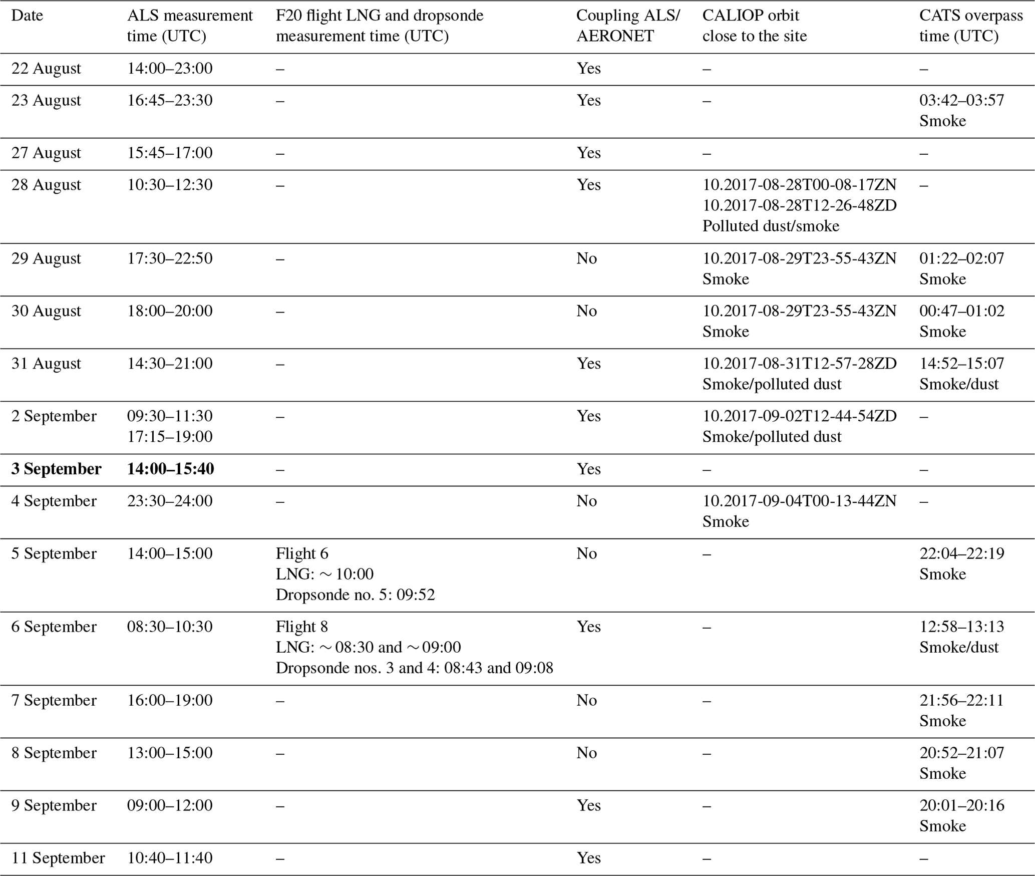
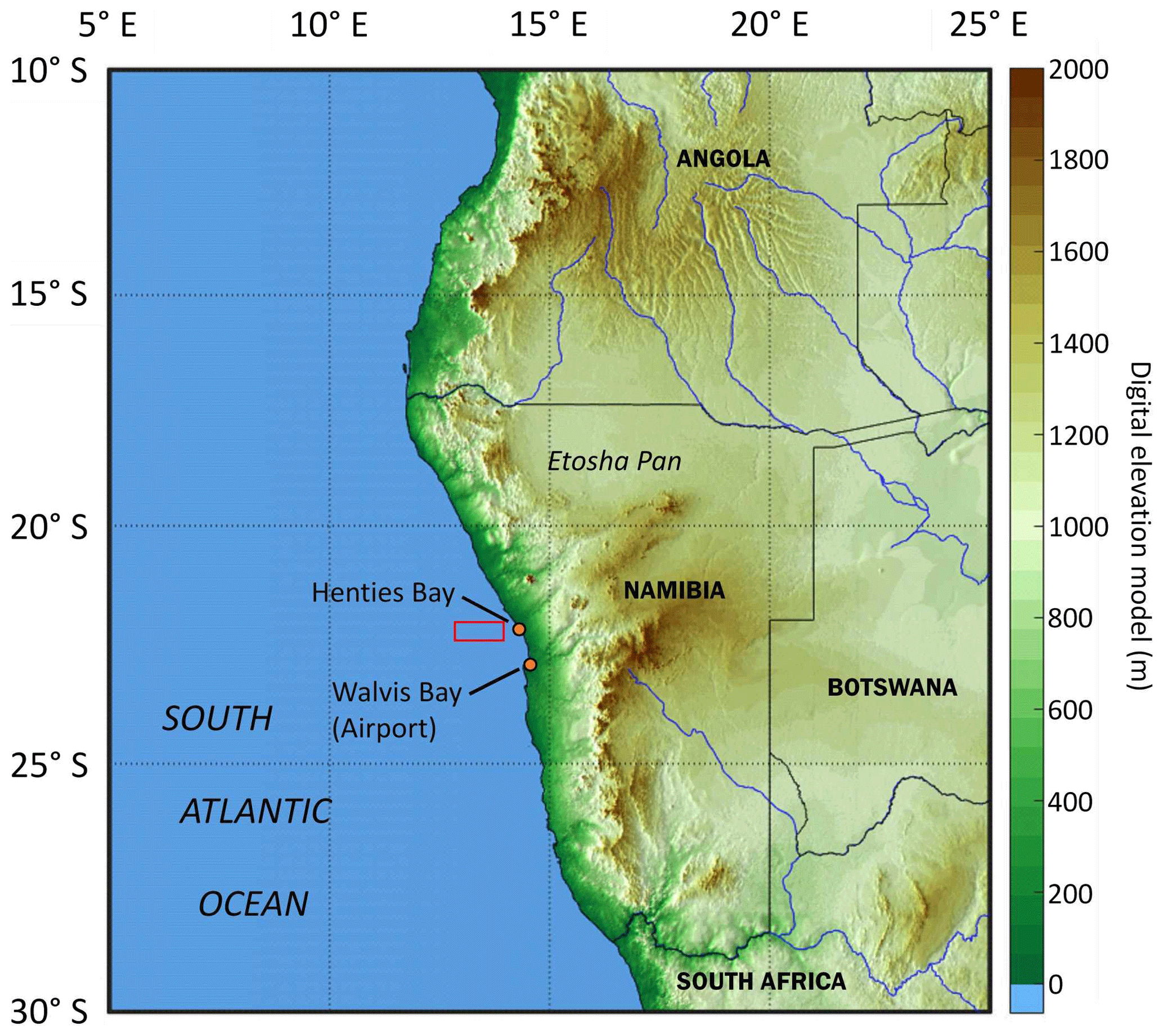
Figure 1Location of the Henties Bay experimental site (in Namibia) on the west African coast. The Walvis Bay airport where the SAFIRE Falcon 20 aircraft operated during AEROCLO-sA is also indicated. The black rectangle surrounds the area chosen to average the MODIS-derived AOTs. The Henties Bay and Walvis Bay locations are marked by orange dots.
2.1 Ground-based lidar
The ALS lidar measurements were carried out continuously between 22 August and 13 September 2017. The data coverage for aerosol study is low because of the quasi-ubiquitous presence of marine stratocumulus and fog during a large part of the observation days. The fog opacity was often such that the laser beam was fully attenuated after a few hundred metres. We therefore considered average profiles taken during periods when no low-level clouds or fog events are observed, i.e. between about 1 and 4 h on a given day (see Table 1). The description of the lidar is given in Appendix A, together with the calibration and data inversion processing.
2.2 AERONET Sun photometer
The site of Henties Bay was equipped with a Sun- and sky-scanning spectral radiometer manufactured by CIMEL Inc. (Paris, France) and belonging to the AERONET automatic and global network of Sun photometers providing long-term and continuous monitoring of aerosol optical, microphysical and radiative properties (http://aeronet.gsfc.nasa.gov/, last access: 23 November 2019). Eight spectral bands are generally used between 340 and 1020 nm. The aerosol optical thickness at the lidar wavelength of 355 nm (AOT355) is assessed using the Ångström exponent (Ångström, 1964) and the Sun photometer AOT at 380 and 440 nm (e.g. Hamonou et al., 1999). We use level-2.0 (cloud-screened and quality-assured) AOT data in the following. The total uncertainty on AOT is for λ>440 nm and for λ<440 nm (Holben et al., 1998). Nevertheless, additional bias may exist when thin clouds are present and not screened in the AERONET level-2 products (Chew et al., 2011). To limit this, ground-based lidar profiles are used to identify the presence of clouds when Sun photometer observations are available.
2.3 Airborne measurements
In this study, we also analyse extinction coefficients over the Atlantic and in the vicinity of Henties Bay, acquired with the LNG lidar (Bruneau et al., 2015) flown on the SAFIRE Falcon 20 on 5 and 6 September. We only use the 532 nm channel because the high level of noise in the high spectral resolution 355 nm channel. Hence, the lidar was operated as a simple backscatter Rayleigh–Mie lidar. The Falcon 20 operated from Walvis Bay, on the western coast of Namibia, roughly 100 km south of Henties Bay where the AEROCLO-sA supersite was located. Details on the Falcon payload as well as the flight plans conducted during these 2 d can be found in Formenti et al. (2019). In addition to the LNG data, we also make use of dynamical and thermodynamical data acquired offshore of Namibia with the Vaisala dropsonde system.
During the first flight (flight no. 6 on the morning of 5 September 2017), the Falcon operated from 07:36 to 10:14 UTC. It flew mostly above the continent to monitor dust emissions over the Etosha Pan (see Formenti et al., 2019). The later portion of the flight was conducted over the sea (from 09:30 to 10:14 UTC), and a dropsonde was launched from 21.69∘ S, 13.78∘ E at 09:52 UTC. For the second flight (flight no. 9 on the morning of 6 September 2017), the Falcon 20 operated from 07:03 to 09:27 UTC and flew over the ocean from 08:20 to 09:27 UTC. Two dropsondes were launched from 19.87∘ S, 11.92∘ E at 08:43 UTC and from 22.23∘ S, 13.41∘ E at 09:08 UTC.
The LNG data over the sea are inverted using the same procedure as for the ground-based ALS lidar (see Appendix A) and utilizing the same LR vertical distribution (see values retrieved in Henties Bay for the 2 d in Sect. 3).
2.4 Space-borne observations
2.4.1 CALIOP and CATS
CALIOP has been flying aboard the Cloud-Aerosol Lidar Pathfinder Satellite Observation (CALIPSO) since 2006 (https://www-calipso.larc.nasa.gov/products/, last access: 23 November 2019). Details on the CALIOP instrument, data acquisition and science products are given by Winker et al. (2007). In this work, we use CALIOP level-2 data version 4.10 (Kim et al., 2018), which was corrected for aerosol types, as noted in Burton et al. (2012). The aerosol types identified in the free troposphere (FT) are typically polluted dust and elevated smoke (see example in Appendix A).
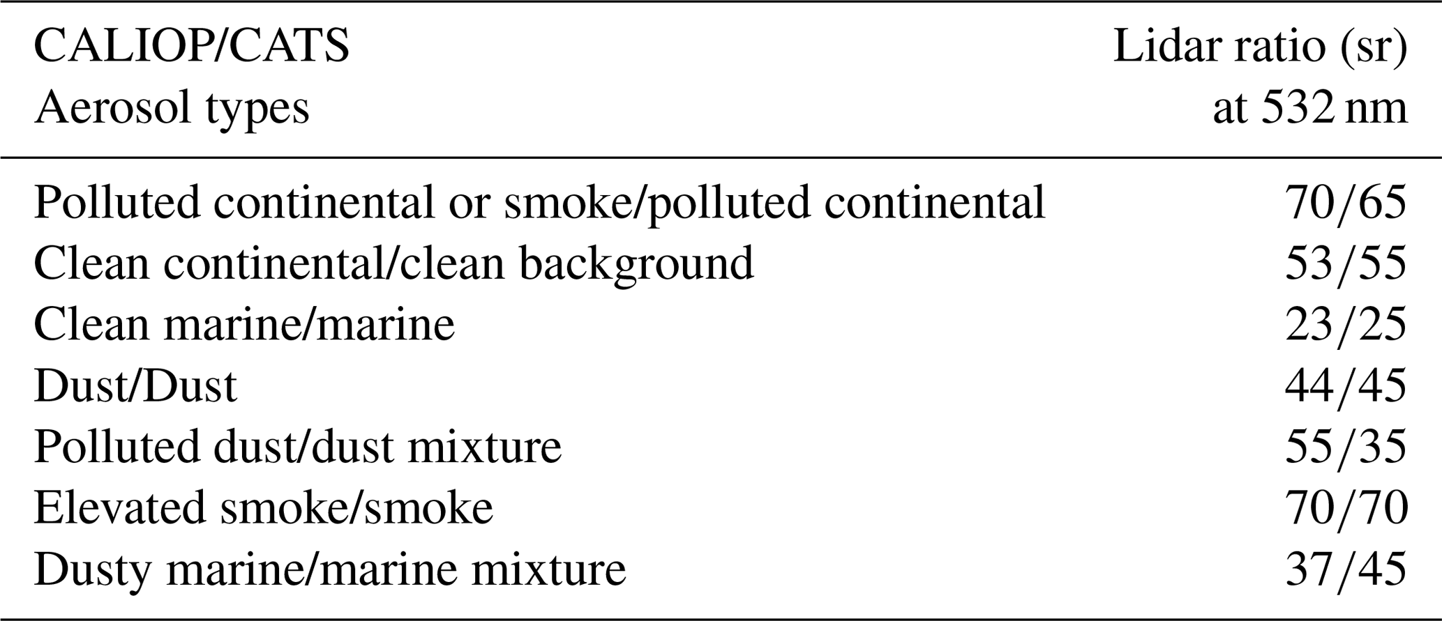
The CATS lidar orbited between 375 and 435 km aboard the non-Sun-synchronous International Space Station (Yorks et al., 2016). It operated between January 2015 and October 2017 with the objective of measuring some cloud and aerosol properties which are useful for climate study. CATS flew over Namibia at various times during the AEROCLO-sA field campaign (Table 1). We mainly used the aerosol types derived from CATS measurements, which are similar to the ones established for CALIOP. The correspondence between the aerosol types derived from CALIOP and CATS measurements is given in Table 2. It should be noted that not all the aerosol types are named exactly in the same way. An example of aerosol types is given in Appendix A.
Table 2LR corresponding with the CATS- and CALIOP-derived aerosol types.
2.4.2 MODIS
The MODIS instruments (King et al., 1992; Salmonson et al., 1989) are aboard the Aqua and Terra platforms (http://modis-atmos.gsfc.nasa.gov, last access: 23 November 2019). The polar orbit of Terra (http://terra.nasa.gov, last access: 23 November 2019) passes over the Equator from north to south in the morning, whereas Aqua (http://aqua.nasa.gov, last access: 23 November 2019) has its ascending node over the Equator during the afternoon. They provide a complete coverage of the Earth's surface in 1–2 d with a resolution between 250 and 1000 m at ground level depending on the spectral band. We use the Terra and Aqua AOT at 550 nm from the MODIS aerosol product level-2 data. Both products are given with a spatial resolution of 10×10 km2 at nadir. The uncertainty in the AOT retrieval (Remer et al., 2005) over land (ocean) is 0.15±0.05 AOT (0.05±0.03 AOT). We will only use data over the sea because Henties Bay is a coastal site affected by the sea breeze and bordered by a strong topography (Fig. 1). This is associated with the lowest levels of uncertainty. The thermal anomalies derived from the MODIS fire product (e.g. Ichoku et al., 2008) are also used (https://modis.gsfc.nasa.gov/data/dataprod/mod14.php, last access: 23 November 2019).
2.5 Modelling
The meteorological patterns are studied using meteorological fields provided by the 6-hourly operational analyses of the European Centre for Medium-Range Weather Forecasts (ECMWF; http://apps.ecmwf.int/datasets/, last access: 23 November 2019, Dee et al., 2011). We also use the near-real-time analyses of atmospheric dynamics and aerosols from the Copernicus Atmosphere Monitoring Service (CAMS; https://atmosphere.copernicus.eu/, last access: 23 November 2019). The calculations for synoptic analysis are computed on a 0.75∘ horizontal regular grid. Daily means are computed by averaging time steps at 03:00, 09:00, 15:00 and 21:00 UTC of daily forecasts initialized at 00:00 UTC. For local analyses, the meteorological wind fields are computed by using 1 h data on a 0.25∘ horizontal regular grid from the fifth ECMWF Reanalysis (ERA5; https://www.ecmwf.int/en/forecasts/datasets/archive-datasets/reanalysis-datasets/ERA5, last access: 23 November 2019; Hoffmann et al., 2019). The back-trajectory analyses are based on the Hybrid Single Particle Lagrangian Integrated Trajectory (HYSPLIT) model (Draxler and Rolph, 2014; Stein et al., 2015). The wind fields used as input from the HYSPLIT model are from GDAS (Global Data Assimilation System; http://www.ncep.noaa.gov/, last access: 23 November 2019) at 0.5∘ horizontal resolution. The isentropic ensemble mode with 24 individual back trajectories is used to take into account the transport trajectory spread associated with the wind field variability around the trajectory's starting point. Using different modelling approaches also allows the consistency of results to be verified.
3.1 Identification of periods from the total AOT
The temporal evolution of the AOT at 550 nm derived from passive remote sensing observations (MODIS and the Henties Bay Sun photometer) and 6 h CAMS fields between 22 August and 9 September 2017 are shown in Fig. 2a. For CAMS, both the AOT extracted from the grid cell centred on Henties Bay and the average AOT calculated on a 3×3 grid-point box surrounding the site are shown. There are little differences between the two CAMS-derived AOTs which highlight the homogeneity of aerosol plumes overpassing Henties Bay according to the model and during that period. The MODIS AOT at 550 nm plotted in Fig. 2a is a daily synthesis of Terra and Aqua products extracted over the sea only (see the black rectangle in Fig. 1), to avoid mixing the effects of coast, topography and surface albedo in the AOT retrievals. Overall, the AOTs from CAMS match within 0.1 the ones derived from both MODIS and the Sun photometer, except on 2 and 7–8 September. These discrepancies on AOT may be also explained by the coarse spatiotemporal sampling of the model, which is insufficient to highlight the sharp variation in AOT due to a very localized aerosol features during these 3 d. As a result, even small differences in the simulation of the weather conditions could lead to substantial differences in AOT for specific locations, especially when AOT values are rather low. Note that no significant precipitation event was recorded during the field campaign, so we can exclude any CAMS misrepresentation of wet deposition processes around Henties Bay. In addition, CAMS simulations show that the AOT is essentially due to organic matter (i.e. biomass burning aerosols); thus, the contribution from non-biomass aerosol can then be excluded as well. On 2 September, a minimum in AOT is observed by the Sun photometer which is not reproduced by CAMS simulations (even though a local minimum in the CAMS AOT can be seen). During this day, the mid-tropospheric circulation was characterized by a low-pressure system located offshore of Henties Bay, juxtaposed with a high-pressure system over southern Africa, resulting in a small river of smoke descending along the coast that CAMS was simulating too far east over Henties Bay. On 7–8 September, the Sun-photometer- and MODIS-derived AOTs were larger than the one computed from CAMS. This could be related to the presence of unscreened optically thin clouds such as the ones observed in the ground-based lidar data on 8 September (Fig. A2d) and/or to the heterogeneity of the meteorological field. Indeed, on 7–8 September, an elongated high pressure dominating over the continent led to the channelling of the smoke from the northwest that is slightly mislocated in the CAMS analyses.
In Fig. 2a, three distinct periods can be identified based on the temporal evolution of both the remote sensing instruments and the CAMS-derived AOT. The optical and geometrical properties of the aerosol layers derived from the remote sensing instruments over Henties Bay during the three periods are summarized in Table 3. The first period (P1; 22–28 August 2017; see Fig. 2a) is characterized by an averaged AOT of ∼0.20 at 550 nm, while for the second period (P2; 28 August–1 September 2017; see Fig. 2a), the AOT increases to ∼0.4. During the third period (P3; 3–11 September 2017), the average AOT is higher than during P2 and around 0.55 at 550 nm (see Fig. 2). Here, 2 September can be considered as a transition period between P2 and P3. The variability of the CAMS-derived AOT is much larger during P3 than during P1 and P2, which may show greater variability in atmospheric transport conditions. The Sun-photometer-derived Ångström exponent (AE) evolves during the period of interest, with AE ∼ 1 during P1 and AE ∼ 1.4 during P2 and P3 (see Table 3), suggesting the presence of larger aerosol in the atmospheric column during P1.
3.2 Aerosol vertical profiles
The AEC profiles shown in Figs. 3 to 7 are obtained in cloud-free conditions using a standard inversion procedure detailed in Appendix A. Most AEC profiles show clear air with low particle concentrations between the planetary boundary layer (PBL) and the elevated aerosol layer, with the notable exception of 2 September in the afternoon, when aerosols are mainly observed in the PBL (Fig. 5b). Figure 2b shows the AOTs at 355 nm calculated from the lidar-derived AEC profiles between the surface and ∼6.5 km a.m.s.l., as well as partial column AOTs in the FT for three different altitude ranges where aerosol loads can be highlighted: namely [1500 3000[, [3000 5000[ and [5000 6000[ m (green, grey and red bars in Fig. 2b, respectively). The temporal evolution of the partial column AOTs corroborates the existence of the three periods. During P3, we observe AOTs in excess of 0.1 between 5000 and 6000 m a.m.s.l. for at least 4 d (3, 6, 7 and 11 September), whereas partial AOTs in that height range are negligible in the previous two periods. AOT values as high as 0.4 are observed on 6 September. The increase in the lidar-derived column AOT (blue bars in Fig. 2b) during P3 is also well correlated with the increase of the partial column AOT in the 1500–3000 m a.m.s.l. interval.
We note a significant increase in terms of the lidar-derived thickness of elevated aerosol layer between the three periods (∼1–2.5 km during P1, ∼2.5–3 km during P2 and ∼2.5–5 km during P3; Table 3) as well as in terms of maximum AEC in the FT (∼0.1 km−1 during P1, ∼0.25 km−1 during P2 and ∼0.3 km−1 during P3; Table 3) as seen in the AEC profiles (compare Fig. 3 for P1 with Fig. 4 for P2). The height of the base of the elevated aerosol layer also increases between P1 and P2, from ∼1 to 1.5 km a.m.s.l. to more than 2 km a.m.s.l. (Table 3), but appears more variable during P3 (from ∼1 to 3 km a.m.s.l.; Figs. 6 and 7). These changes in optical and geometrical properties of the aerosols in the FT are related to the variability of long-range transport over the area, as discussed in Sect. 5.
CALIPSO and CATS retrievals suggest differences in the FT aerosols between P1/P2 and P3, with more occurrence of polluted dust (55 sr) in P1/P2 and polluted continental or smoke (70 sr) in P3. In the PBL, during P1/P2, the retrieved low value of LR (i.e. 23 sr) required to reproduce the Sun photometer AOT is consistent with the presence of clean marine aerosols in the PBL (e.g. Flamant et al., 2000). The retrieved higher LRs required in P3 indicate the presence of other aerosol types, which may include smoke (i.e. 70 sr) or a mixture of smoke and terrigenous aerosols (i.e. 55 sr). The latter LR value suggests the presence of terrigenous aerosols mixed with smoke, corresponding to the aerosol type “polluted dust”. During P3, aerosols in the FT are mainly identified as “smoke” (based on the CALIOP and CATS types). Very few Sun photometer data are available for LR retrieval due to the quasi-permanent presence of cloud cover over Henties Bay during the cycles of almucantar measurements. Nevertheless, such a measurement could be obtained during P3 on 3 September 2017 at ∼ 14:10 UTC. A Sun-photometer-derived LR of ∼63 sr at 532 nm has been computed from the backscatter phase function and the single scattering albedo (Dubovik et al., 2000). It was found to match the LR associated with the smoke type of CALIOP and CATS (i.e. 65–70 sr at 532 nm).
The PDR is computed for each AEC profile given in Figs. 3 to 7. The PBL is associated with the lower PDR (i.e. < 2 %–3 %), mainly during P1 and P2. This argues for the presence of hydrophilic spherical particles as marine aerosols. Within the free troposphere, the PDR is higher, mainly between 5 % and 10 %, and may correspond to a mixing of biomass burning and dust aerosols as often observed in biomass burning aerosol plume over others areas (e.g. Chazette et al., 2016; Kim et al., 2009). This is consistent with the hypothesis of dust mobilization and mixing by convection in biomass burning regions. Above the PBL, larger PDR can be observed and may indicate a higher relative presence of dust. This should be taken with caution, as AEC values are low for these layers and uncertainties are therefore higher.
Table 3Properties of aerosol layers above the Henties Bay site as derived from the ground-based lidar, CALIOP, CATS, the Sun photometer and MODIS: lidar ratios selected for the free troposphere (LRFT; in bold) and the planetary boundary layer LRPBL at 355 nm, ground-based lidar (GBL)-derived AOTGBL at 355 nm and its uncertainty (detection noise and atmospheric variability), Sun-photometer-derived AOTphot at 355 and 550 nm, Sun-photometer-derived Ångström exponent (AE), MODIS-derived AOTMODIS in 0.5∘ × 0.5∘ area over the sea close to Henties Bay, free troposphere aerosol (FTA) layer thickness and bottom height and maximum of the aerosol extinction coefficient (AECmax) in the FTA. P1 and P2 correspond to periods when the AFT is mostly composed of “polluted dust”, and P3 corresponds to the period when smoke aerosols dominate the composition of the UAL.
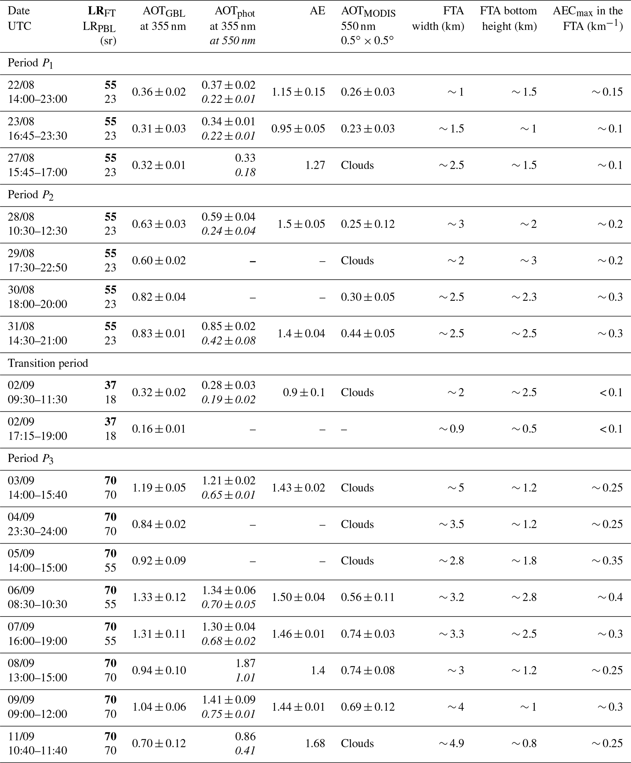
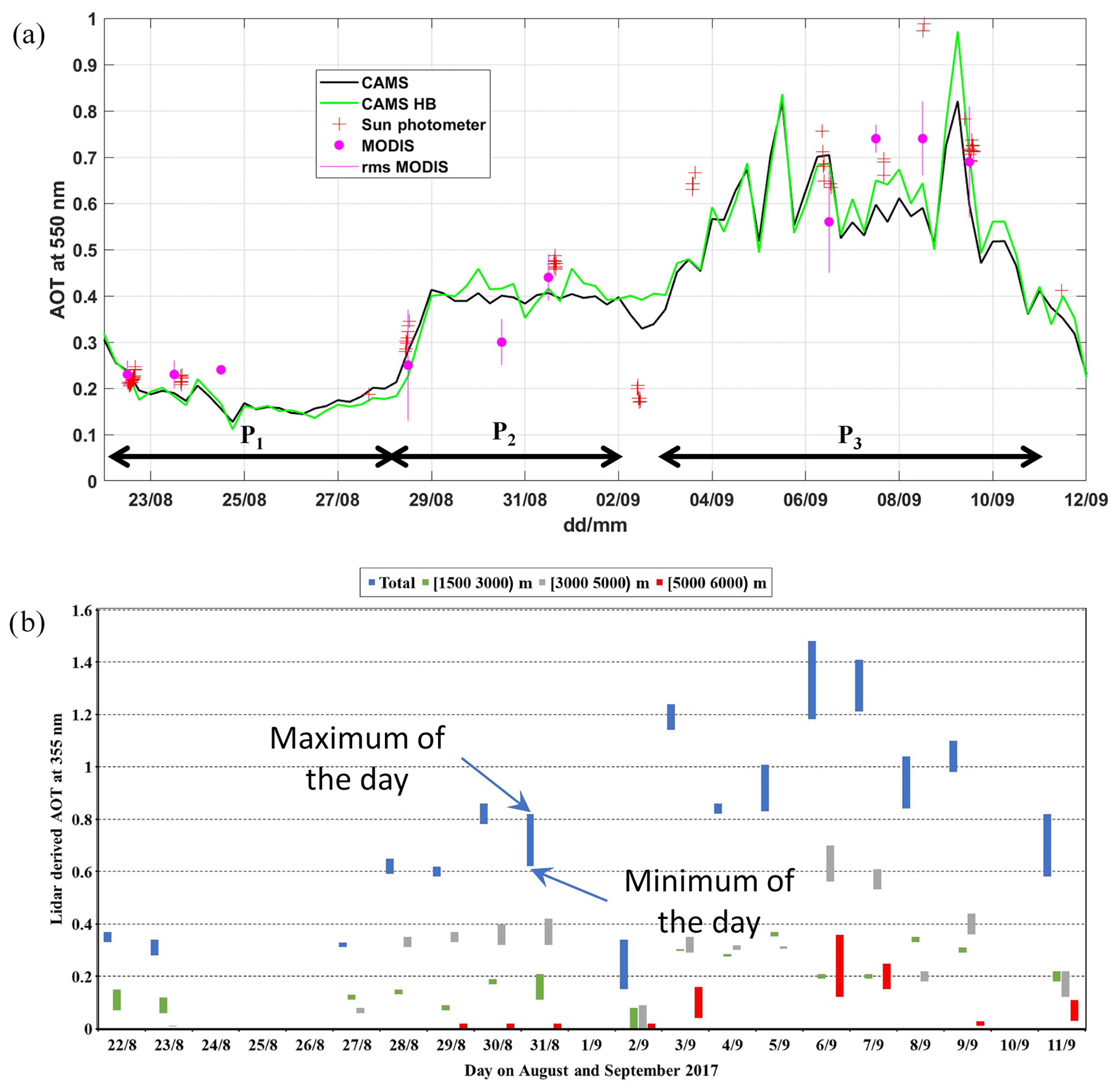
Figure 2(a) Temporal evolution of the AOT at 550 nm derived from CAMS (solid black and green lines), Sun photometer (red crosses) and MODIS (magenta dots) data. The solid green line shows CAMS AOT extracted on the grid cell centred on Henties Bay. The solid black line shows the CAMS AOT averaged over nine grid cells (a 3×3 grid box) centred on Henties Bay. The three periods highlighted by the AOT values (P1, P2 and P3) are indicated. (b) Temporal evolution of the lidar-derived AOT at 355 nm for the altitude ranges [1500 3000[ m in green, [3000 5000[ m in grey and [5000 6000[ m in red. The total AOT is given in blue. The vertical bars delimit the daily extremes of AOT.
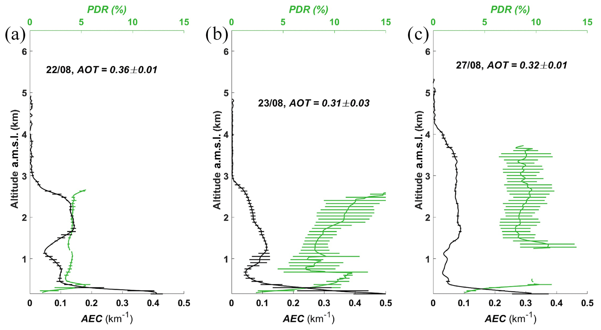
Figure 3Vertical profiles of the aerosol extinction coefficient (AEC) and particle depolarization ratio (PDR) at 355 nm with their uncertainties (horizontal bars) for period P1 on (a) 22 (14:00–23:00 UTC), (b) 23 (16:45–23:30 UTC) and (c) 27 (15:45–17:00 UTC) August 2017. The total AOT at 355 nm is also given for each profile with its uncertainty.
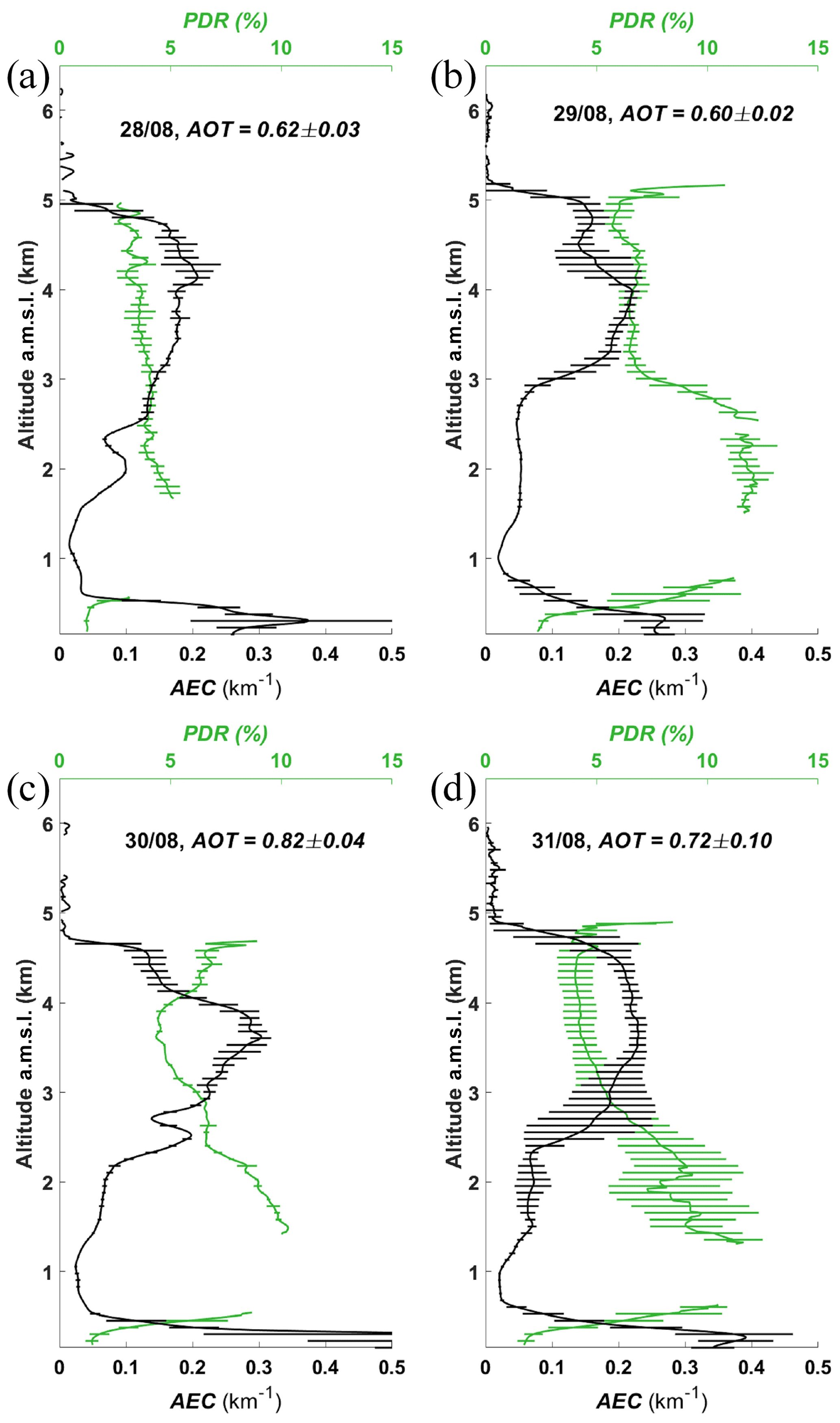
Figure 4Vertical profiles of the AEC and PDR at 355 nm with their uncertainties (horizontal bars) for period P2 on (a) 28 (10:30–12:30 UTC), (b) 29 (17:30–22:50 UTC), (c) 30 (18:00–20:00 UTC) and (d) 31 (14:30–21:00 UTC) August 2017. The total AOT at 355 nm is also given for each profile with its uncertainty.
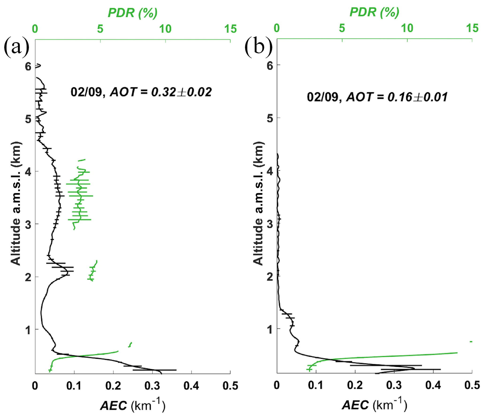
Figure 5Vertical profiles of the AEC and PDR at 355 nm with their uncertainties (horizontal bars) for the transition period on 2 September 2017 at (a) 09:30–11:30 UTC and (b) 17:15–19:00 UTC. The total AOT at 355 nm is also given for each profile with its uncertainty.
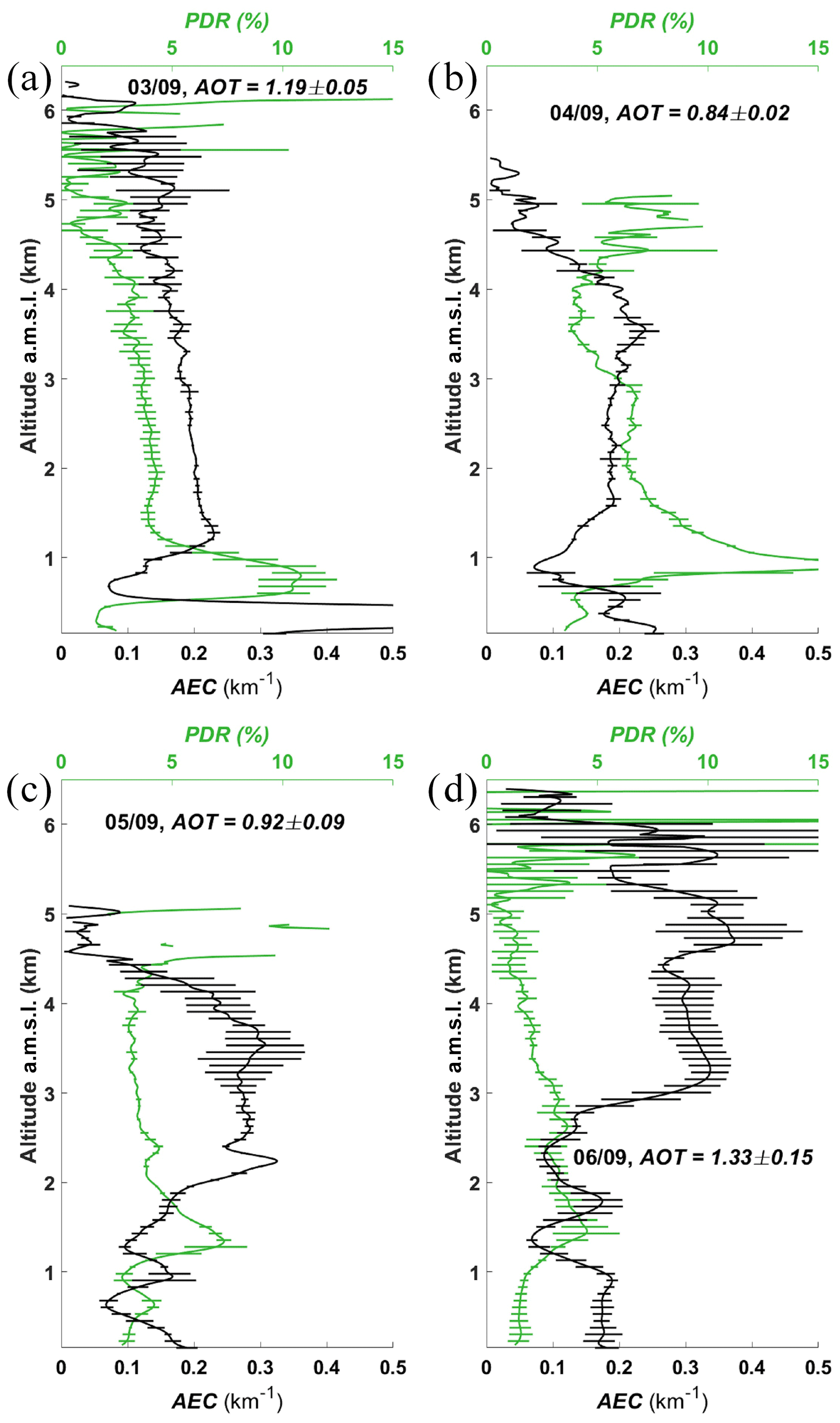
Figure 6Vertical profiles of the AEC and PDR at 355 nm with their uncertainties (horizontal bars) for period P3 on (a) 3 (14:00–15:40 UTC), (b) 4 (23:30–24:00 UTC), (c) 5 (14:00–15:00 UTC) and (d) 6 (08:30–10:30 UTC) September 2017. The total AOT at 355 nm is also given for each profile with its uncertainty.
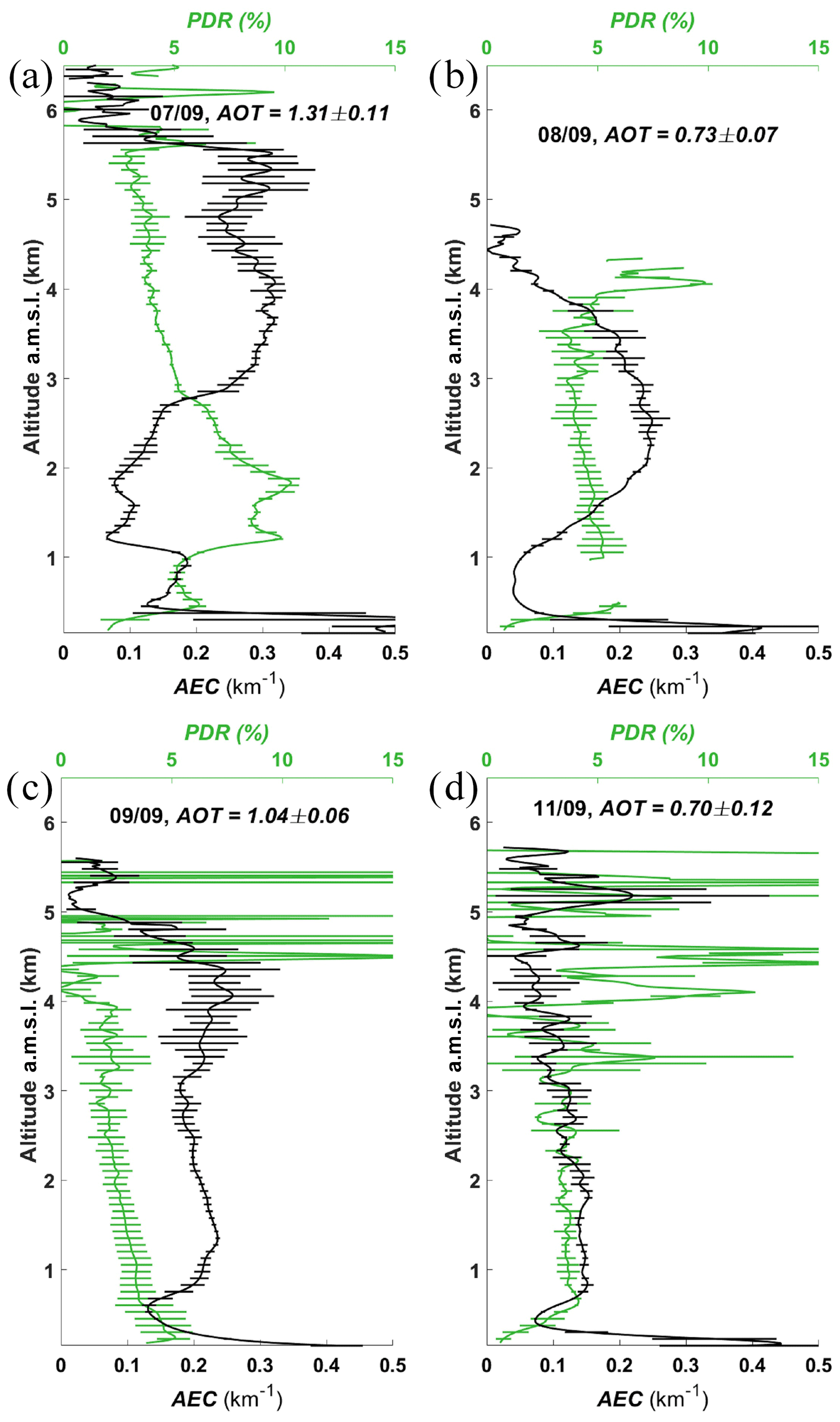
Figure 7Vertical profiles of the AEC and PDR at 355 nm with their uncertainties (horizontal bars) for period P3 on (a) 7 (16:00–19:00 UTC), (b) 8 (13:00–15:00 UTC), (c) 9 (09:00–12:00 UTC) and (d) 11 (10:40–11:40 UTC) September 2017. The total AOT at 355 nm is also given for each profile with its uncertainty.
The purpose of this section is to highlight the spatial variability of the vertical structure of aerosols in the vicinity of Henties Bay through an analysis of the airborne lidar observations acquired offshore during two flights on 5 and 6 September 2017. Note that airborne observations during AEROCLO-sA were only made during period P3 (Formenti et al., 2019).
4.1 Flight on 5 September 2017
Figure 8a shows the time–space cross section of the LNG-derived apparent aerosol backscatter coefficient (ABC) profiles at 532 nm along the Falcon 20 flight track on the morning of 5 September 2017 following the methodology by Chazette and Totems (2017). LNG data highlight the presence of a widespread elevated BBA layer over the area of interest. The inversion of the LNG ABC data is performed using the same LRs as for the inversion of the ground-based lidar in Henties Bay (70 sr in the FT and 55 sr in the PBL; see Table 3). The average LNG-derived AEC profile shown in Fig. 8b is obtained over the ocean between the two vertical dotted black lines in Fig. 8a around 10:00 UTC. Figure 9 shows the comparison between the dropsonde profiles of temperature, wind and relative humidity (RH) located over the ocean in Fig. 8a and their counterparts extracted from ERA5 at 10:00 UTC in a 0.25∘ × 0.25∘ grid centred on the Henties Bay site. There is a very good agreement between the vertical wind profiles (intensity and direction); nonetheless, the wind is a little stronger on the dropsonde vertical profile, especially around 2 km a.m.s.l., above the marine PBL, where it is in excess of 20 m s−1 (and less than 15 m s−1 in ERA5). The dropsonde measurements provide evidence of a very sharp RH gradient at the top of the BBA layer (from 80 % to nearly 1 %–2 %; Fig. 9b) at 6 km a.m.s.l., this gradient being collocated with the large vertical gradient of AEC at 532 nm seen in the LNG data (Fig. 8b). They also provide evidence of a minimum of RH above the PBL, around 2 km a.m.s.l., roughly coinciding with the base of the BBA layer (∼2.2 km a.m.s.l.; Table 3). The high RH values in the elevated BBA layer may be associated with the large amounts of water vapour released during combustion in wildfires (Clements et al., 2006; Deaconu et al., 2019; Parmar et al., 2008). The high RH may also be characteristic of continental air, whereas low-humidity air above may be associated with subsiding tropical or midlatitude air that has been depleted of moisture via prior precipitation. The sharp RH gradient at the top of the BBA layer is not well represented in the ERA5 analysis. The depth of the marine PBL is also seen to be thicker in the observations than in the model (Fig. 9b), possibly because the ERA5 profile is partly over the Namibian coast. The airborne lidar data highlight the presence of stratocumulus over the ocean around 1 km a.m.s.l. (Fig. 8b, the absence of lidar data below that height indicating that the laser beam is completely extinguished in the cloud), close to the maximum of RH observed with the dropsonde (Fig. 9b).
When comparing the mean vertical distribution of aerosols from the LNG-derived AEC profile offshore and the ground-based lidar AEC profile in Henties Bay averaged between 14:00 and 15:00 UTC (Fig. 8b, the two profiles being separated by ∼100 km), we observe differences in terms of the altitude of the BBA layer top. Note that (i) since the two lidars operate at different wavelengths, the AEC intensity is not directly comparable, but the vertical structure of AEC profiles is, and (ii) there is a 4 h difference between the aircraft profiles and the mean profile over Henties Bay. On the other hand, we see that the bottom of the BBA layer is located at roughly the same altitude (Fig. 8b). Furthermore, ERA5 analyses also highlight the fact that the dynamical and thermodynamical structure of the lower troposphere over Henties Bay did not evolve significantly between 10:00 and 15:00 UTC (not shown), except for an increase of RH between 5 and 6 km a.m.s.l. (by 20 %, coherent with the appearance of clouds as seen in Fig. A2c) and of wind speed at 4.5 km a.m.s.l. (by 5 m s−1). Rather, the difference may be explained by the regional-scale circulation in the mid-troposphere across the area. Over the ocean, ERA5 data indicate stronger northwest winds (∼23 m s−1) at the location of the airborne lidar AEC profile compared to the wind over Henties Bay (12 m s−1) for the entire day on 5 September (not shown). The resulting horizontal wind shear between the Namibian coast and the ocean leads to differential advection within the BBA layer and a different vertical structure of the aerosol layer between the coastline and over the ocean.
4.2 Flight on 6 September 2017
During the flight on 6 September 2017 (Fig. 10a), LNG observations were made further offshore than on the previous day. In Fig. 10b, we compare the AEC profiles acquired with LNG to the west and the northwest of Henties Bay (marked “1” and “2”, respectively, in Fig. 10a) at ∼ 08:30 and ∼ 09:00 UTC, with the average AEC profile obtained between 07:00 and 09:30 UTC from the ground-based lidar in Henties Bay. Differences in the structure of the BBA layer appear between the vertical profiles west of Henties Bay (profile “1” in Fig. 10a) and the one further north (profile “2” in Fig. 10a). The shape of the elevated BBA layer observed from the AEC profiles in “1” and in Henties Bay matches the structure of the RH and wind speed profiles from the southernmost dropsonde (Fig. 11b), with a top (base) altitude of 5 km (3 km) a.m.s.l. The wind in the BBA layer is observed to be rather constant and equal to 17 m s−1 on average as well as coming from the north. The maximum RH in the FT is ∼55 % and observed near the top of the BBA layer (Fig. 11b), while small RH values (less than 10 %) are seen above ∼6 km a.m.s.l. It is worth noting the presence of a slightly enhanced RH layer between 5.5 and 6 km a.m.s.l., where enhanced lidar-derived AEC values are also observed in Henties Bay (Fig. 10b). The elevated BBA layer is separated from the PBL by a rather dry layer with small AECs, characterized by a strong wind shear (Fig. 11b). The apparent height of the PBL observed in the AEC profile in Henties Bay agrees with the location of the gradient in RH.
AEC profile “2” derived from LNG observations and obtained ∼100 km north of profile “1” exhibits a different structure than that of Henties Bay. The top of the BBA layer is observed to be slightly higher (5.2 km a.m.s.l.), while the altitude of the base of the BBA layer is the same (∼3 km a.m.s.l.). The wind speed in the BBA layer as seen from the northernmost dropsonde (Fig. 11a) is weaker than when it is off Henties Bay (Fig. 11b), while the RH is higher throughout the lower troposphere, especially below the elevated BBA layer. The LNG profile in “2” exhibits significant AEC values below 3 km a.m.s.l. corresponding to the base of the BBA layer observed further south, which may be partly related to the impact of RH on aerosol optical properties. A deep moist layer (including the PBL) is observed below the BBA layer.
In addition to the important variability in terms of vertical structure of the AEC profiles, it should be noted that the 550 nm AOT derived from the Sun photometer in Henties Bay (0.70±0.05) is significantly higher than those determined from the airborne lidar data at 532 nm in “1” (0.37±0.06) but also significantly lower than that measured in “2” (1.13±0.10). This variability is also reflected in the vertical distribution of aerosols above 5 km a.m.s.l., where non-negligible contributions to the AOT are observed in Henties Bay (with 0.15 < AOT < 0.35 at 355 nm; Fig. 2b) and in “2” (with AOT 0.08 at 532 nm). Such a contribution was even more marked on the previous day in the LNG observations (see Fig. 10b), with an AOT at 532 nm above 5 km a.m.s.l. in excess of ∼0.05.
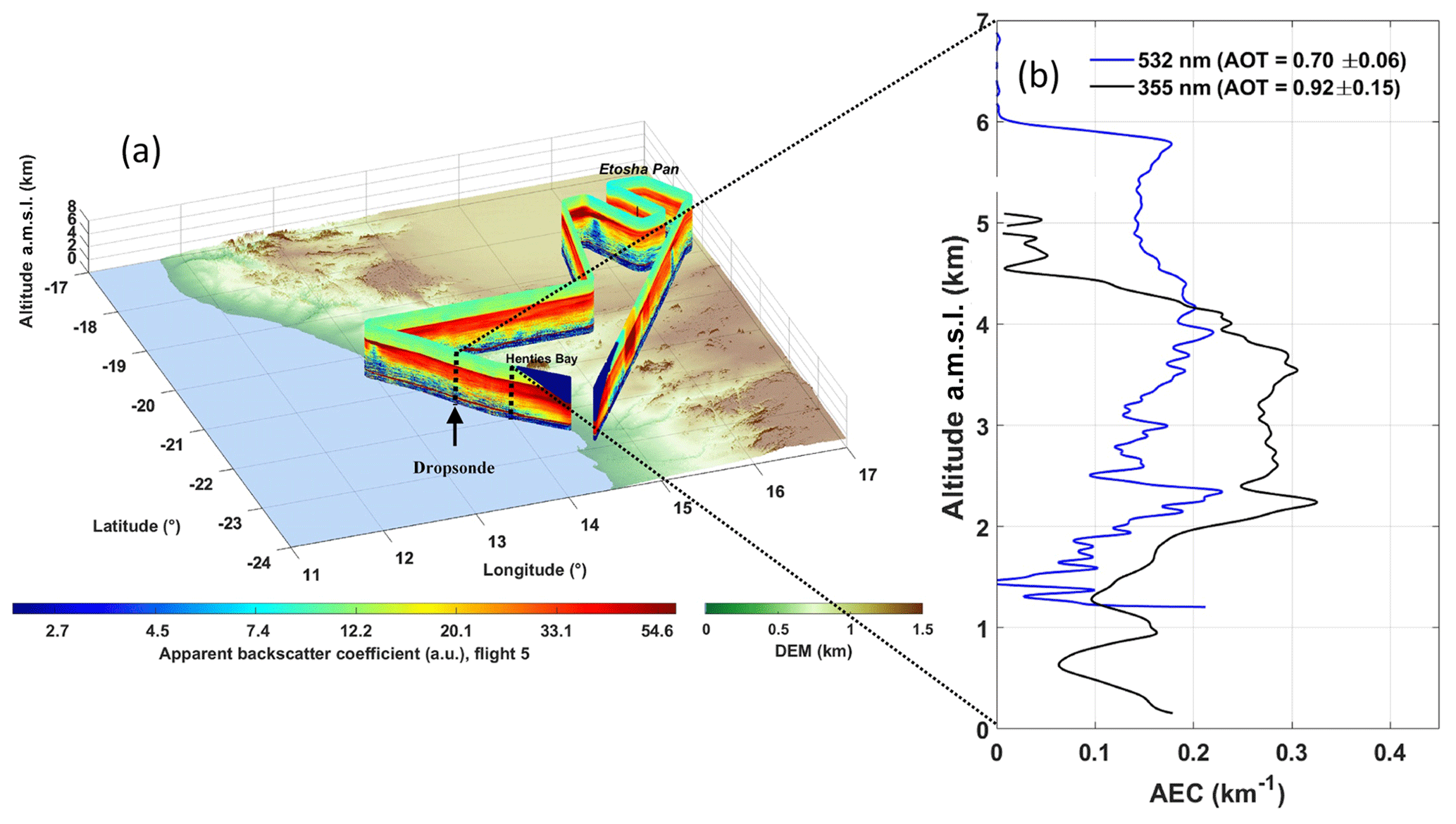
Figure 8(a) Distance–height (“curtain-like”) evolution of the LNG-derived apparent backscatter coefficient at 532 nm below the SAFIRE Falcon 20 during the morning flight on 5 September 2017. The location of the dropsonde released over the ocean is indicated as well as the location of the averaged LNG AEC profile shown in panel (b) (between the two dotted vertical lines). (b) Vertical profiles of the AEC derived from the airborne lidar at 532 nm (∼ 10:00 UTC; solid blue line) and from the ground-based lidar at 355 nm (∼ 14:00–15:00 UTC; solid black line).
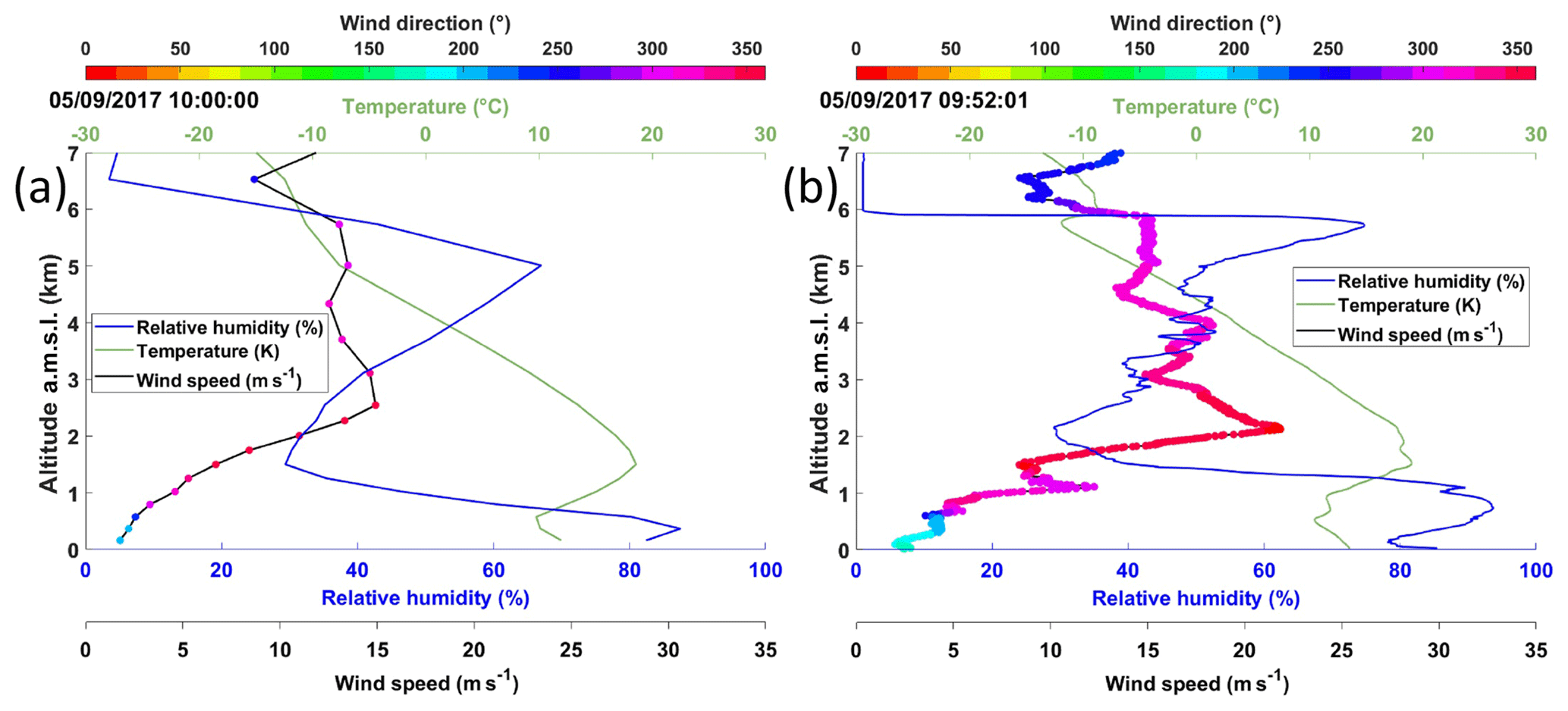
Figure 9(a) Wind speed (solid black line), wind direction (coloured dots), RH (solid blue line) and temperature (solid green line) profiles extracted from ERA5 at 10:00 UTC above Henties Bay over a 0.25∘ by 0.25∘ grid. (b) Same as panel (a) but measured by the dropsonde released over the ocean at 09:52 UTC on 5 September 2017.
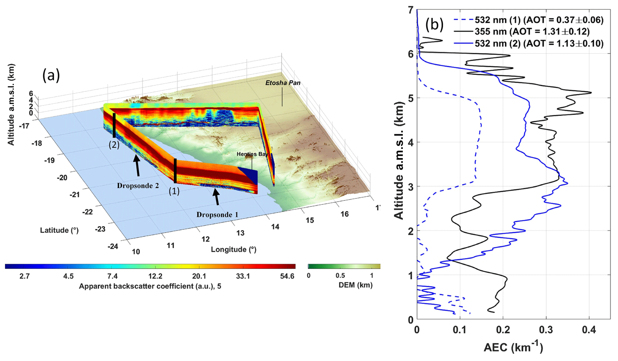
Figure 10(a) Same as Fig. 6a but on 6 September 2017. The locations of the two launched dropsondes are also indicated by arrows. The lidar AEC profile labelled “1” shown in panel (b) is obtained after inversion of the LNG observations averaged between the two locations of the two dropsondes. The AEC profile labelled “2” is obtained after inversion of the lidar data between the northernmost dropsonde and the northern end of the Falcon leg. (b) Vertical profiles of the AEC derived from the airborne lidar at 532 nm (∼ 08:30 and ∼ 09:00 UTC, for profile “2” (solid blue line) and “1” (dashed blue line), respectively) and from the ground-based lidar at 355 nm (∼ 07:00–09:30 UTC; solid black line).
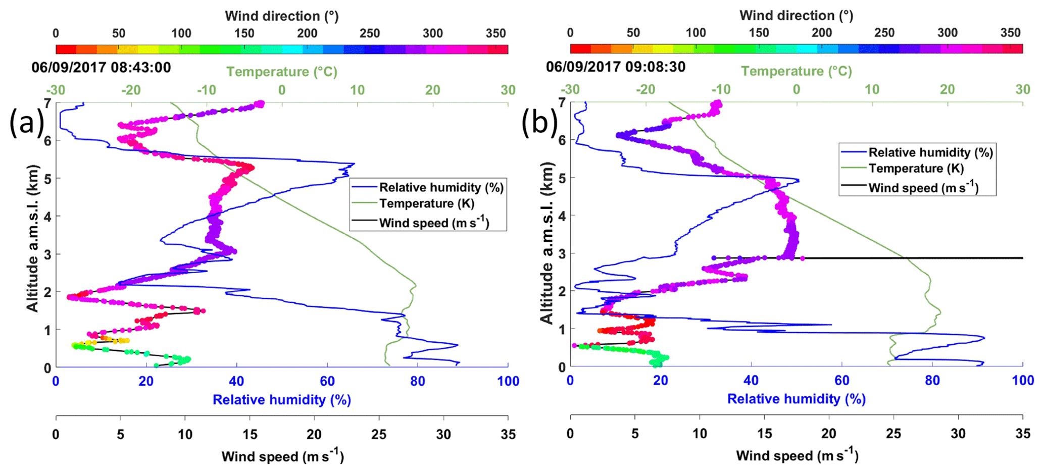
Figure 11(a, b) Same as Fig. 7b but for the dropsondes released at 08:43 UTC (to the northwest of Henties Bay; dropsonde no. 2 in Fig. 10a) and at 09:08 UTC (west of Henties Bay; dropsonde no. 1 in Fig. 10a).
5.1 RH as indicator of changing synoptic conditions
Figure 12 shows the time–height evolution of hourly RH profiles from ERA5 between 22 August and 9 September 2017 at Henties Bay. The three periods (P1, P2 and P3) identified from the AOT (Fig. 2) are seen to correspond to distinct RH conditions in the mid-troposphere, with rather dry conditions during P1, then increased RH below 5 km a.m.s.l. during P2 and even more humid conditions below 6 km a.m.s.l. during P3. For instance, the RH values between 2.5 and 5 km a.m.s.l. increase from values below 10 % to values in excess of 60 % between P1 and P2, which is most probably associated with the transport of BBA over Henties Bay. Likewise, the RH values between 5 and 6 km a.m.s.l. increase from 5 % to ∼70 %–80 % between P2 and P3, which is an indication that the meteorology has changed and that the origin of air masses may be different. Periods P2 and P3 are clearly separated by an episode of very dry RH conditions on 2 September, the day also corresponding to a minimum of AOT over Henties Bay (Fig. 2). In general, the location of the elevated aerosol layer in the vertical corresponds to the highest RH as previously observed from airborne measurements. In the following, we designed back-trajectory analyses to investigate the origin of the air masses in the FT.
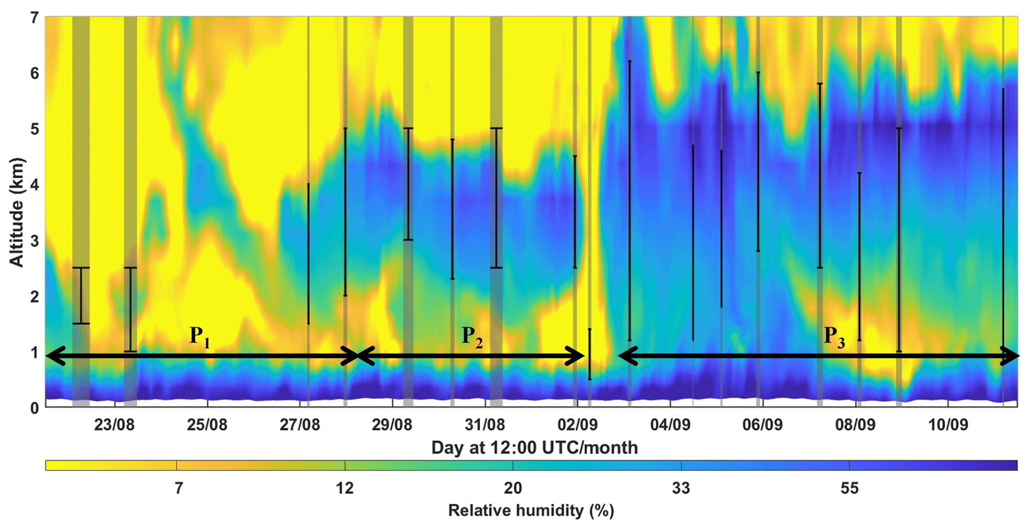
Figure 12Time–height evolution of the relative humidity vertical profiles derived from ERA5 above Henties Bay. The vertical grey lines indicate the time of the ground-based lidar profiles shown in Figs. 3–7. The thickness of the grey lines depends on the averaging period (the thicker the line, the longer the average). The three periods highlighted by the AOT values (P1, P2 and P3) are also indicated. The black vertical lines show the lidar-derived altitude location of the aerosol layer.
5.2 Air mass pathway change during the three periods
A statistical study of the back trajectories of air masses originating from Henties Bay was designed to analyse the circulations related to the three identified periods (P1, P2 and P3). The 6 d back trajectories are initialized at 12:00 UTC using the ensemble mode of the Lagrangian HYSPLIT model for which 27 isentropic trajectories are calculated for each selected altitude point over Henties Bay. Altitudes are discretized every 250 m between the base height (∼1500 m a.m.s.l.) and the maximum top height (∼6000 m a.m.s.l.) of the BBA layers. A composite of the back trajectories is then made for the three different periods by calculating the probability of trajectories passing through each grid point with a spatial resolution of 0.5∘. This statistical approach makes it possible to consider the dispersion of back trajectories that can be linked to complex atmospheric circulations. The altitude ranges selected for releasing the back trajectories are derived from the structure of the elevated aerosol layer given in Table 3 and Figs. 3–7. They are the same for the three periods in order to facilitate comparison: [1500 3000[ m a.m.s.l., [3000 5000[ m a.m.s.l. and [5000 6000[ m a.m.s.l. To visualize the results, we used the two-dimensional histograms presented in Figs. 13–15.
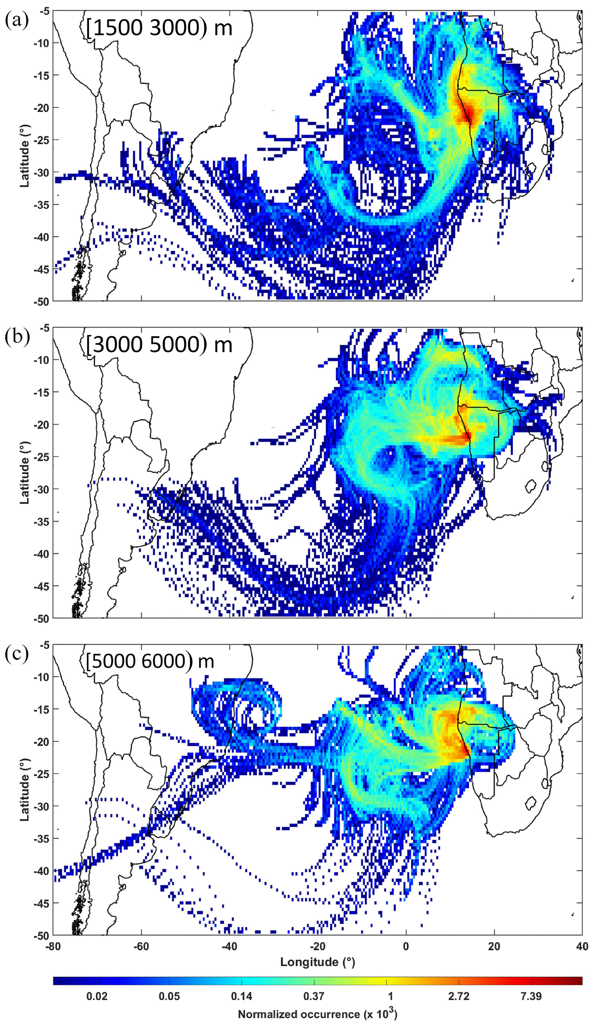
Figure 13Normalized occurrence of the back trajectories starting over Henties Bay at 12:00 UTC during period P1 from the altitude ranges of [1500 3000[ (a) [3000 5000[ (b) and [5000 6000[ m a.m.s.l. (c). The calculations have been made using 6 d isentropic back trajectories with the HYSPLIT model (courtesy of NOAA Air Resources Laboratory; http://www.arl.noaa.gov, last access: 23 November 2019) in ensemble mode. The normalization is performed with respect to the total number of pixels for a horizontal resolution of 0.5∘.
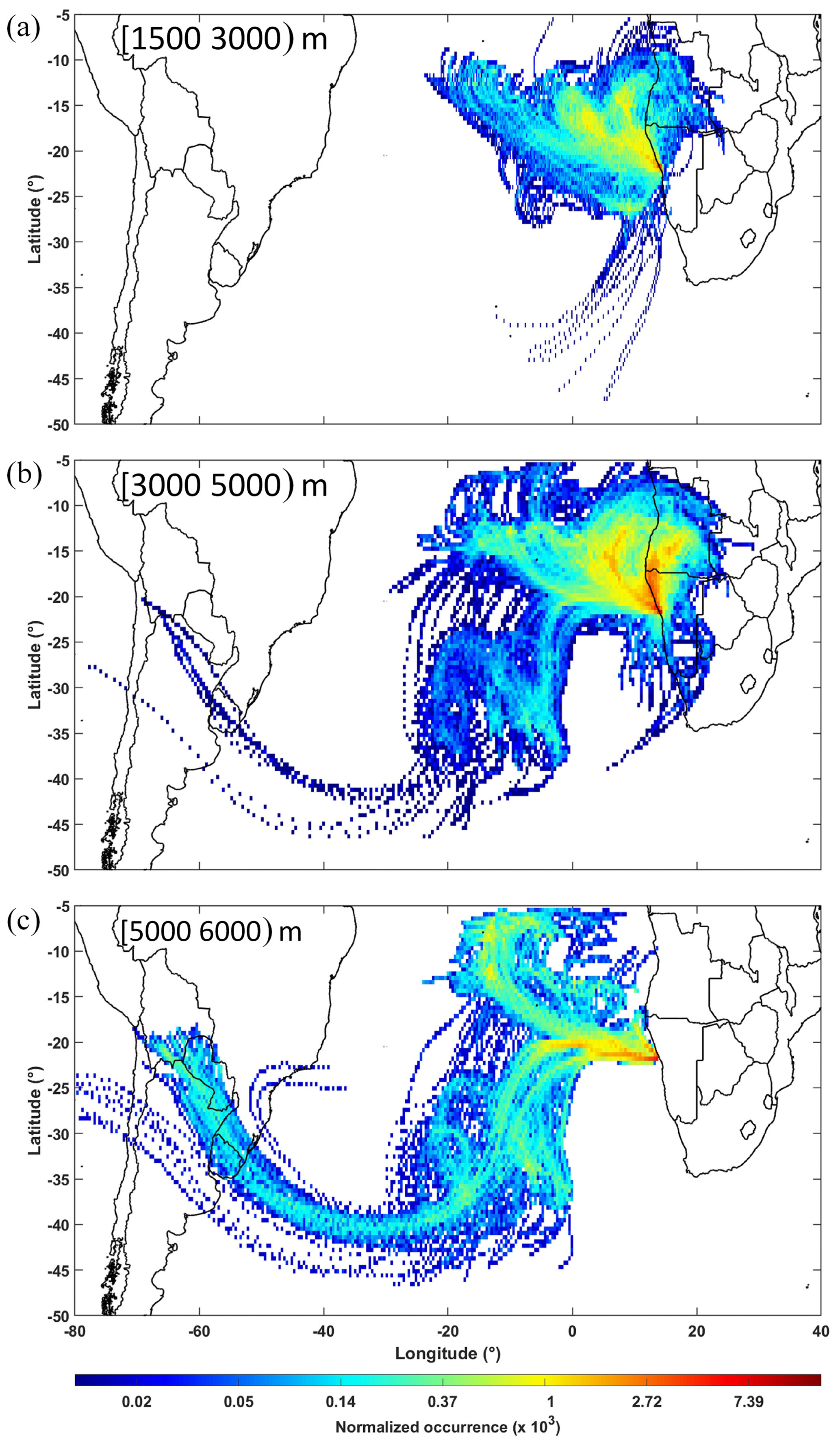
Figure 14Normalized occurrence of the back trajectories starting over Henties Bay at 12:00 UTC during period P2 from the altitude ranges of [1500 3000[ (a) [3000 5000[ (b) and [5000 6000[ m a.m.s.l. (c). The calculations have been made using 6 d isentropic back trajectories with the HYSPLIT model (courtesy of NOAA Air Resources Laboratory; http://www.arl.noaa.gov, last access: 23 November 2019) in ensemble mode. The normalization is performed with respect to the total number of pixels for a horizontal resolution of 0.5∘.

Figure 15Normalized occurrence of the back trajectories starting over Henties Bay at 12:00 UTC during period P3 from the altitude ranges of [1500 3000[ (a) [3000 5000[ (b) and [5000 6000[ m (c). The calculations have been made using 6 d isentropic back trajectories with the HYSPLIT model (courtesy of NOAA Air Resources Laboratory; http://www.arl.noaa.gov, last access: 23 November 2019) in ensemble mode. The normalization is performed with respect to the total number of pixels for a horizontal resolution of 0.5∘.
5.2.1 Period P1
During P1, the density of trajectories is highest to the north of Henties Bay and particularly along the Angolan and Namibian coastlines (Fig. 13). The distribution of the trajectories suggests that the aerosols observed over Henties Bay mainly originate from Angola and northern Namibia (close to the back trajectories' starting point) and are transported towards the observational supersite. Considering the altitude of the back trajectories, plausible injection heights over Angola are highly variable and may reach ∼5 km a.m.s.l. to explain the vertical structures of lidar profiles. There are also many trajectories coming from over the southern Atlantic Ocean. For the altitude range [3000 5000[ m a.m.s.l., some trajectories arriving on 25 August in Henties Bay are seen to originate from southern Brazil 6 d earlier, a region where fires are detected by MODIS between 16 and 21 August. It should be noted that BBA would have needed to be injected to heights between 5 and 7 km a.m.s.l. in order to be transported to Henties Bay on 25 August. Nevertheless, no lidar measurements are available during this day to confirm this possible alley of cross-Atlantic transport. For the altitude ranges [5000 6000[ m a.m.s.l., no significant aerosol layer is observed by the ground-based lidar (Fig. 3).
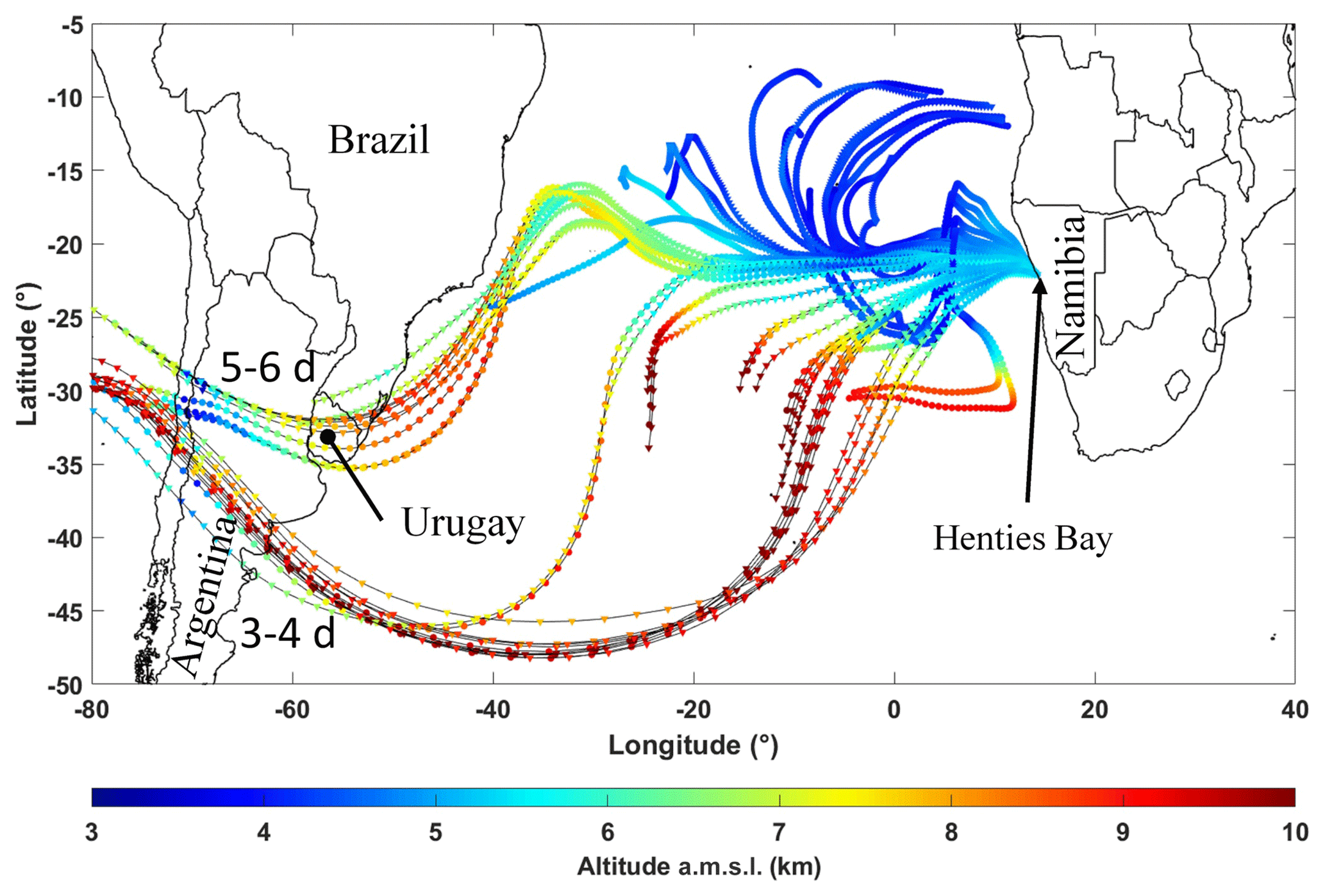
Figure 16The 6 d isentropic back trajectories starting over Henties Bay on 6 September at 12:00 UTC. They are computed by the HYSPLIT model (courtesy of NOAA Air Resources Laboratory; http://www.arl.noaa.gov, last access: 23 November 2019) in ensemble mode. The time to arrival above the South America is indicated. The altitude of back trajectories along the route is given by the colour bar.
5.2.2 Period P2
During P2 (Fig. 14), the density of trajectories is also high along the Namibia coastline north of Henties Bay between 1500 and 5000 m a.m.s.l. and over the ocean. The distribution of trajectories suggests that the BBAs observed in Henties Bay mainly are advected within the altitude range [3000 5000[ m a.m.s.l. from central Angola and have travelled a few hundred kilometres over the ocean before being transported back towards the southern African coastline. This constitutes the main contribution of the lidar-derived AEC profiles, provided that the injection heights over Angola can reach 5 km a.m.s.l., as suggested by the CALIOP and CATS observations (see Fig. A3). As for P1, we observed no significant aerosol contribution above 5 km a.m.s.l. (Fig. 4). The contributions from South America are due to air masses arriving over Henties Bay on 30 and 31 August between 3 and 5 km a.m.s.l. These air masses have the possibility to import biomass burning aerosols emitted 6 d before from northern Argentina and injected at altitudes close to 4 km a.m.s.l. according to back trajectories. Such injection heights are often observed via CALIOP over South America. The lidar observations over Henties Bay do not show any significant AEC features above 5 km a.m.s.l., in spite of the possibility of cross-Atlantic transport highlighted by the back trajectories. This could be related to a lack of fires in the region overpassed by the trajectories or injection heights in the biomass burning regions that are below the altitude of the transport associated with the trajectories. It may also be the case that BBAs are subject to wet deposition along the trajectories as air masses experience precipitation associated with the weather systems over the Atlantic Ocean.
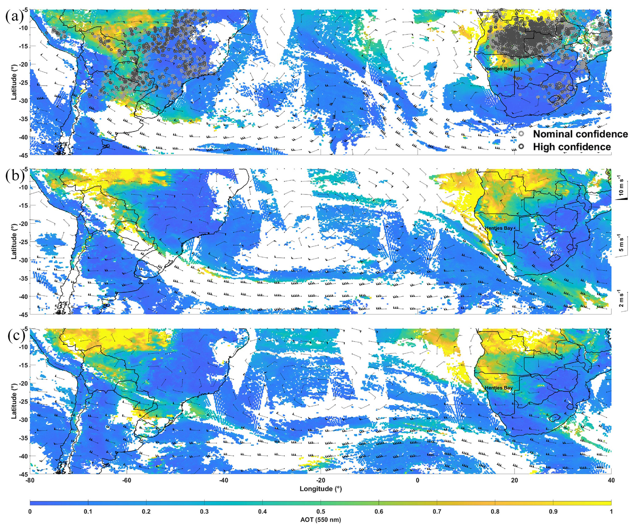
Figure 17MODIS-derived AOT at 550 nm on (a) on 3 September 2017 with wildfire hotspots over both southern Africa and South America, (b) on 5 September 2017 and (c) 6 September 2017. The ERA5 wind fields at 500 hPa on each day have been added in black.
5.2.3 Period P3
During P3 for the three altitude ranges, the occurrence of trajectories (Fig. 15) is highest along the northern Namibian coast, over the land. This suggests a more direct transport from the anthropogenic fire and/or wildfire areas in Angola than during P2 and P1, which may explain the highest AOTs for the third period. The occurrence of trajectories over the ocean just west of the southern African coast suggests that a significant part of the aerosols arriving in Henties Bay have travelled over the Atlantic Ocean before being transported back towards the continent. This constitutes the main contribution of the lidar-derived AEC profiles below 5 km a.m.s.l., provided that the injection heights over Angola can reach that height over the continent. Above 5 km a.m.s.l., significant AEC features are observed with the lidar (Figs. 6 and 7) that reliably contribute to the AOT (∼10 %–15 %; Fig. 2b). According to Fig. 15c, such features could be related to transport from Angola, provided that BBAs are injected sufficiently high over the biomass burning areas. Figure 15c also shows that a significant number of trajectories reaching Henties Bay come from South America. For instance, more trajectories originating from the South American burning zones are also seen over the southern Atlantic Ocean for the altitude range [5000 6000[ m than during the two other periods. Several transport pathways from South America to southern Africa are observed for this altitude range: (i) two southern routes where trajectories go as far south as 48∘ S for the first one and 40∘ S for the second one before moving equatorward towards Namibia, (ii) a northern route where trajectories first follow the eastern coast of Brazil before heading due east towards Namibia and (iii) a more direct eastward route across the Atlantic before turning counter clockwise towards Henties Bay. Back trajectories suggest that air mass transport from South America along the last three more northern routes took 5–6 d to reach Henties Bay, whereas the transport along the more southern route only took 3–4 d.
5.3 Possible contribution to the AOT from South America during P3
We now look specifically at the P3 period during which a large number of trajectories coming from South America are seen compared with the two other periods. Some of the aerosol layers observed during P3 between 5 and 6 km a.m.s.l. by the ground-based lidar, and in particular those associated with the highest AOTs on 6 and 7 September 2017 (Fig. 2b), may be associated with biomass burning over Angola but also with fires occurring on 1–4 September 2017 over southern Brazil, northern Argentina and Uruguay.
The back trajectories shown in Figs. 13–15 are calculated assuming isentropic transport. However, this hypothesis is not necessarily verified during the studied period. Indeed, when trajectories cross the Atlantic Ocean, they encounter more a baroclinic fluid than a barotropic fluid due to the presence of strong low-pressure centres such as the cut-off low. The potential temperature is therefore no longer necessarily a tracer of the air mass and isentropic trajectories can quickly diverge towards higher altitudes. This is shown in Fig. 16 on 6 September (the same is true on 7 September). Nevertheless, some trajectories pass under 5 km a.m.s.l. over northern Argentina. The same trajectory simulation conducted with an isobaric hypothesis on 6 and 7 September shows that all the back trajectories come from Argentina for altitudes that remain in the range of biomass burning injection heights (∼5 km a.m.s.l.). However, isobaric trajectories are not necessarily more representative than isentropic trajectories (Stohl, 1998).
MODIS-derived AOTs (Fig. 17) highlight the existence of an aerosol plume over the ocean along the northern fringe of a large cloud band. The locations of fires over South America are also indicated in Fig. 17a for 3 September 2017. The BBAs seem to be advected across the Atlantic Ocean along two main routes also identified in the previous back-trajectory analyses (Sect. 5.2.3). The northernmost one follows the coast of Brazil before heading straight towards Namibian coasts. The poleward one follows the strong winds at 500 hPa along the western flank of high pressure centred over the eastern coast of Brazil (Fig. 17a). A mid-tropospheric westerly jet then transports the aerosol plumes over the Atlantic Ocean where they are then advected northward around the eastern edge of the high-pressure system located over the Atlantic Ocean. The ubiquitous cloud cover along the southern and eastern fringes of the high-pressure system does not allow the retrieval of AOTs with MODIS, except offshore of the Rio de la Plata estuary and at the edge of cloud fields caught in the west–east circulation. The northward progression of the air masses transporting the BBA along the coast is further accelerated by the presence of a poleward moving cut-off low (centred at 40∘ S, 15∘ W) separating from the westerlies further south (Fig. 17a). Over the following days, the cut-off low is seen to merge back with the westerlies while progressing eastward, and the high-pressure system at 500 hPa is observed to also move over the Atlantic Ocean and merge with the St. Helena high on 5 September (Fig. 17b). The mid-tropospheric westerly jet may transport the aerosols issued from biomass burning over South America along the southern fringe of the St. Helena high, which is centred at ∼25∘ S and ∼20∘ W. The jet is seen to extend quite far east over the Atlantic Ocean and to almost reach the southern tip of southern Africa (Fig. 17c). Some aerosols travelling along the southern route may be redirected towards Namibia by the strong northerly flow along the eastern flank of the St. Helena high.
Furthermore, the temporal variability of BBA transport patterns from South America to southern Africa may be related to the variability of the Southern Annular Mode (SAM; i.e. the north–south movement of the westerly wind belt around Antarctica). Indeed, Trenberth (2002) shows that the SAM is the main driver of extratropical circulation in the Southern Hemisphere on weekly to decennial timescales, which is also the main driver of climate variability, affecting anthropogenic fire and/or wildfire activities over South America (e.g. Holz et al., 2017). For instance, positive phases of the SAM (i.e. when a band of westerly winds contracts toward Antarctica) are associated primarily with warm conditions in the forested areas of South America, thereby favouring biomass burning events. On the other hand, negative phases lead to an expansion of the wind belt towards the lower latitudes, leading to the possibility for BBA transported in the westerlies to reach southern Africa in the austral winter. Given the possible short timescale of variability of the SAM, it is likely that the transport patterns to Henties Bay identified during period P3 are related to a negative SAM phase, while during P1 they are related to a positive phase. On longer timescales, climate modelling studies indicate a robust positive trend in the SAM for the end of this century (Lim et al., 2016), so climate conditions conducive to an impact of the widespread South American fire activity in southern Africa will likely continue throughout the 21st century. However, further studies are needed to support this conclusion, which will have to be based on longer observation periods involving lidar technology.
During the intensive field campaign of the AEROCLO-sA project (22 August–12 September 2017), the very persistent cloud cover topping the marine boundary did not allow continuous ground-based monitoring of the aerosol layers above the stratocumulus deck in the mid-troposphere. Nevertheless, the available lidar observations performed over the coastal site of Henties Bay allowed to highlight three contrasted periods of biomass burning aerosol transport (P1, P2 and P3). The inversion of the ground-based lidar profiles was carried out using the constraints provided by the aerosol types of the CALIOP and CATS space-borne instruments but also the photometric measurements from AERONET network. The latter showed an overall good agreement with the MODIS AOT observations and the AOT outputs of the CAMS model. Differences were noted in the presence of high aerosol content (AOT at 355 nm > 0.8) between the lidar- and Sun photometer-derived AOTs, but those were likely due to the presence of clouds that were not detected by the passive sensors.
Combining observations and back-trajectory analyses, we highlight the existence of three periods with very different transport modes towards Henties Bay during the field campaign. The lowest AOTs (< 0.2 at 550 nm) of the first period (P1) are associated with air masses from Angola travelling along the Namibian and Angolan coasts. Intermediate AOTs (∼0.4 at 550 nm) of the second period (P2) are associated with polluted dust (i.e. dust mixed with biomass burning aerosols from Angola), as well as dust from the Etosha Pan, which is recirculated above the ocean. During the third period (P3), the largest AOTs (∼0.7 at 550 nm) are observed, mainly due to more direct transport from the Angola burning areas with an aerosol plume extending vertically between 1.5 and ∼6 km a.m.s.l. The atmospheric composition in the free troposphere for this period is the most variable in the time. We show a possible contribution of forest fire aerosols from South America (south of Brazil, Argentina and Uruguay) with plumes transported to Henties Bay around 5000–6000 m a.m.s.l. and mainly observed on 6 and 7 September, with a contribution to the total AOT of ∼10 %–15 %. The aerosol plume from South America could be advected across the Atlantic Ocean along a route following the strong westerlies of the southern fringes of the St. Helena high before heading north toward Namibia in connection with an equatorward-moving cut-off low.
To the authors' knowledge, this is the first time that the evolution of the optical properties of aerosols in the FT over coastal Namibia is characterized, in relation to different transport regimes. The main contribution of the BBA from Angola and the arguably smaller contribution of the South American anthropogenic fires and/or wildfires to the atmospheric aerosol composition over the Namibian coast were shown. The synergy between active and passive remote sensing observations performed from ground-based and space-borne platforms, together with back-trajectory analyses, was essential to provide these conclusions.
The aircraft and ground-based data used here can be accessed using the AEROCLO-sA database at http://baobab.sedoo.fr/AEROCLO/ (last access: 6 December 2019). An embargo period of 2 years after the upload applies. After that, external users can access the data in the same way as AEROCLO-sA participants before that time. Before the end of the embargo period, external users can request the release of individual datasets. It is planned for AEROCLO-sA data to get DOIs, but this has not been carried out for all datasets yet. The back-trajectory data can be obtained upon request to the first author of the paper.
A1 Description of the ground-based lidar
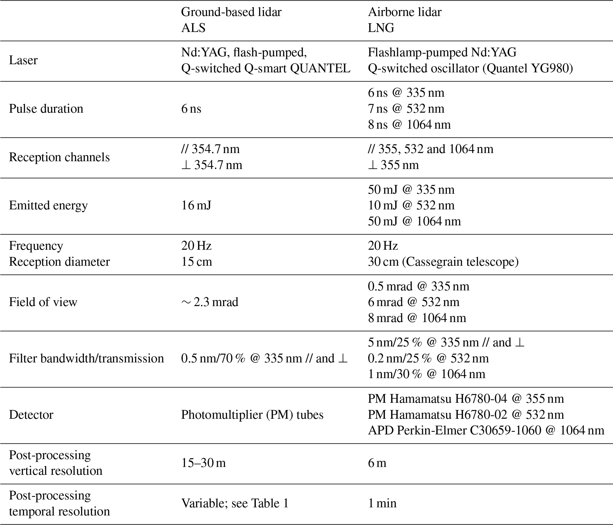
The ground-based lidar system used at the Henties Bay site is the ALS450® lidar manufactured by Leosphere and initially developed by the Commissariat à l'Energie Atomique (CEA) and the Centre National de la Recherche Scientifique (CNRS) (Royer et al., 2011a). The lidar emission is based on an Ultra® Nd:YAG laser manufactured by Quantel, delivering 6 ns width pulses at the repetition rate of 20 Hz with a mean pulse energy of 16 mJ at a wavelength of 355 nm. This system is particularly well adapted to measure tropospheric aerosol profiles in the lower and middle troposphere. Its high vertical resolution of ∼15 m after filtering and temporal resolution (∼1 min) gives the advantage of being able to follow the fast vertical evolutions of the atmospheric scattering layers and to accurately locate the aerosol layers within the troposphere. The lidar is composed of two receiver channels dedicated to the measurement of the co-polar and cross-polar signals. The detection is carried out by photomultiplier tubes and narrowband filters with a bandwidth of 0.5 nm. Its main characteristics are summarized in Table A1, where we have added the features of the LNG lidar for comparison.
A2 Overlap correction and rightness of lidar profiles
In order to derive AEC profiles, the lidar ABC in the aerosol-free portions of the vertical profiles must be assessed and must follow the slope of the molecular backscattering. The ABC, also called the total attenuated backscatter coefficient (Royer et al., 2011a), corresponds to the raw lidar signal corrected for both the contribution of the sky background and the solid angle, as in Eq. (3) of Royer et al. (2010).
Furthermore, close to the lidar emission source, the overlap factor generated by the overlap defects of the laser emission and telescope reception fields also needs to be assessed. The overlap factor is derived from measurements acquired in the horizontal line of sight, with the hypothesis of a homogeneous atmosphere along the line of sight between the emission and a distance of 1.5 km. The overlap factor and the associated standard deviation are shown in Fig. A1. It can be considered that the correction of the overlap factor induces a relative error lower than 15 % for an overlap factor between 0.8 and 1 (Chazette, 2003), corresponding to a distance of 150 m from the emitter. The molecular contribution is obtained from the ERA5 pressure and temperature data at the horizontal resolution of 0.25∘ using the Nicolet model (Nicolet, 1984). The error on the aerosol extinction coefficient due to uncertainty on the molecular density remains below 2 %–3 % (Chazette et al., 2012b). The main sources of uncertainty are the shoot noise and the atmospheric variability during the measurement. Both are taken into account for each retrieved profile.
A representative time-average lidar profile of the ABC over the duration of the measurement field campaign is shown in Fig. A2. The dates were chosen to be representative of the dataset of vertical lidar profiles encountered during the AEROCLO-sA campaign. The curves in black are the ABC profiles and those in red correspond to the molecular backscatter coefficient computed using ERA5 data. We note that in the top of the profiles there is a very good agreement that ensures that the lidar is well aligned. The area comprised between the black and red curves corresponds to the contribution of atmospheric aerosols and, in the upper part of the profiles, to that of optically thin clouds (Fig. A2c and d). The aerosol content increases rapidly between 22 and 28 August, showing a significant evolution of aerosol contributions in the free troposphere (FT) between 1 and 5 km a.m.s.l. It is notable that the vertical profiles of the ABC vary little during the averaging period; the average profiles are therefore quite representative of the state of the atmosphere for all the considered periods.
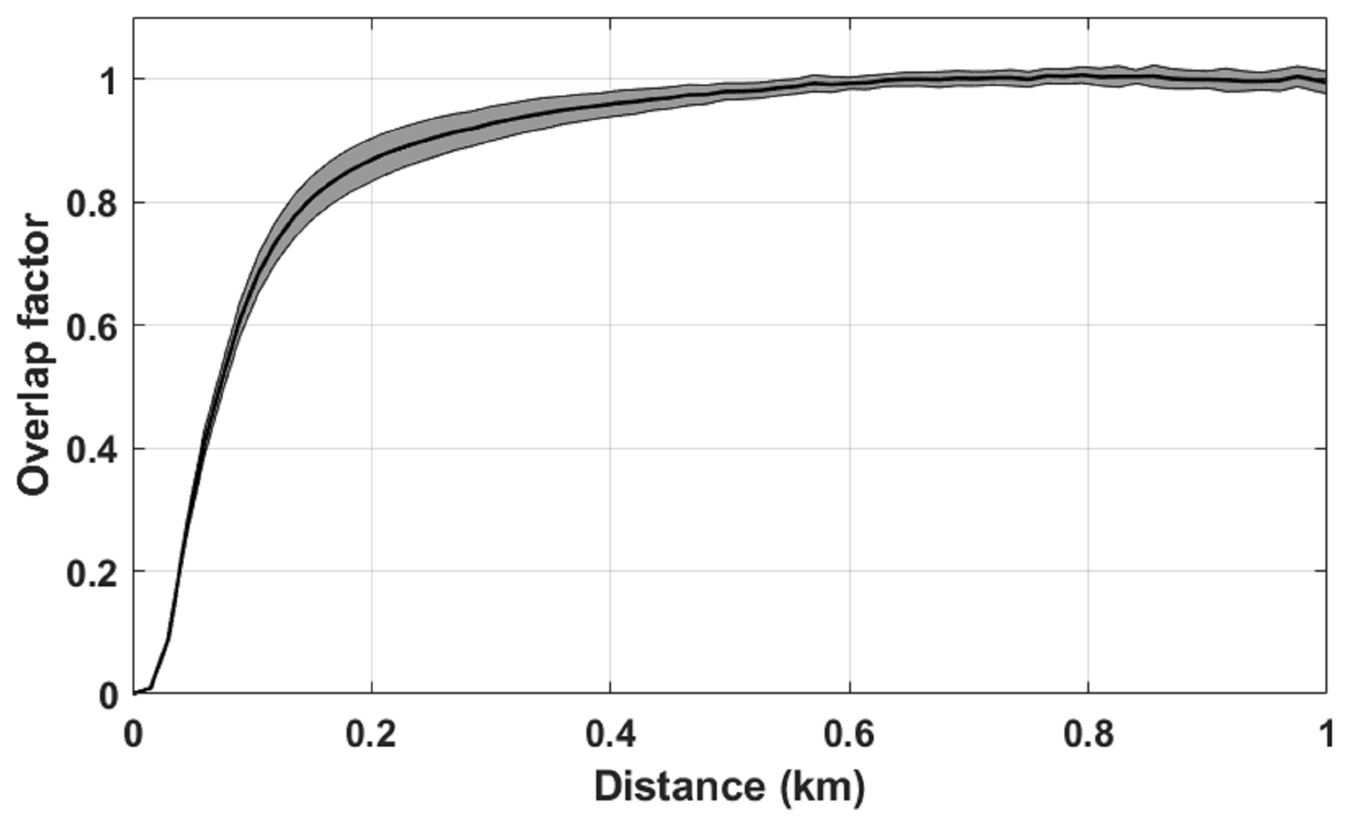
Figure A1Overlap factor of the ALS (continuous black line) and its standard deviation (grey area).
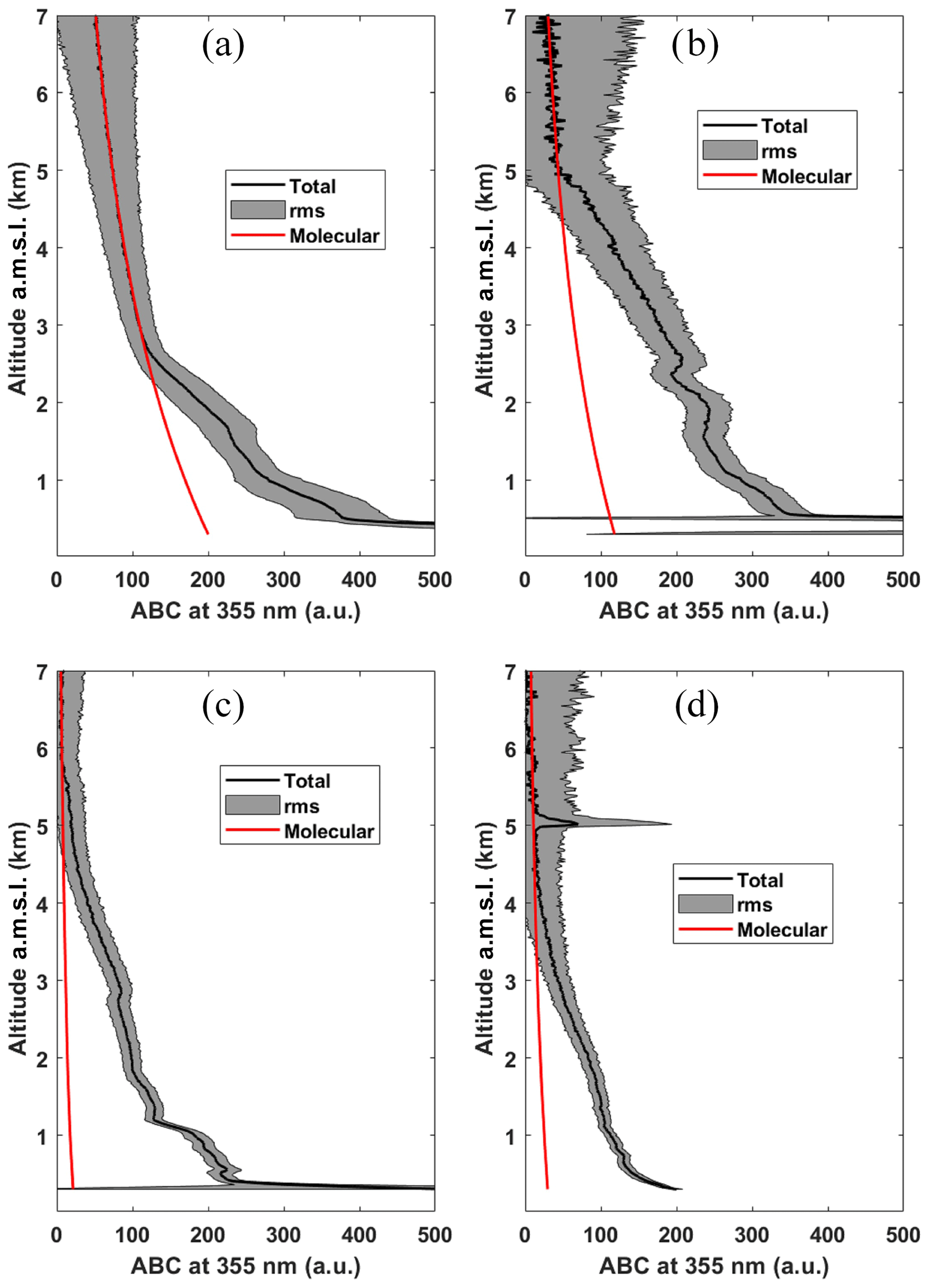
Figure A2Apparent backscatter coefficient (solid black lines) profiles obtained from the ALS lidar in Henties Bay on (a) 22 August 2017 between 14:00 and 23:00 UTC, (b) 28 August 2017 between 10:30 and 12:30 UTC, (c) 7 September 2017 between 16:00 and 19:00 UTC, and (d) 8 September 2017 between 13:00 and 15:00 UTC. The red lines correspond to the molecular backscatter coefficient computed using ERA5 data. The grey area is the standard deviation linked with the statistical error (the shoot noise and the atmospheric variability).
A3 Ground-based lidar data processing using external constraints
The inversion procedure to retrieve the aerosol optical properties from ALS is well documented in previous articles where uncertainty sources are exhaustively quantified (e.g. Raut and Chazette, 2009; Royer et al., 2011b; Chazette et al., 2012a). In the present case, where a simple elastic backscattering lidar is used, we use additional constraints to the lidar equation using Sun-photometer-derived AOT when available but also the aerosol types determined from the CALIOP and CATS measurements for cases where the orbit allowed the sampling of aerosols present in the FT. Figure A3 gives the example of the case of the geographical coincidence between the nighttime CALIOP (CATS) orbit on 28 (30) August 2017 and the lidar measurements above the Henties Bay site. All available CALIOP and CATS orbits passing over Namibia were analysed, and the results in terms of aerosol types are given in Tables 1 and 2. The correspondence in terms of LR is given in Table 2 for both instruments.
In the area of interest, aerosol properties are different in the planetary boundary layer (PBL), where the composition is dominated by marine and coastal dust emissions, and in the FT where the composition is dominated by long-range transport of BBA and dust emitted over the continental plateau. Therefore, we have used different values of LR in the PBL and in the FT to perform the lidar inversion when lidar measurements were acquired concomitantly with Sun photometer AOT measurements. The LR in the FT is derived from the aerosol types performed by the space-borne lidars (see Table 2). When there is no CALIOP or CATS overpasses, we take the value of LR of the nearest day also considering the shape of the AEC profile and the origin of air masses using back trajectories. Values of 65–70±25 sr and 55±25 sr at 532 nm are used for the two main aerosol types sampled, namely smoke and polluted dust, respectively. The ground-based lidar in Henties Bay operates at 355 nm; the LR value is then different. Müller et al. (2007) showed that LR values at 355 and 532 nm differ by about of 20 % for forest fire smoke and less than 10 % for dust aerosols (see Table 1 of their paper), widely included in the expected uncertainty in LRs for space-borne lidar. In the PBL, the LR values are selected from the discrete set of lidar ratios shown in Table 2 via a minimization of the difference of AOT between the ground-based lidar and the Sun photometer: the LR in the PBL is adjusted so that the AOT calculated from the lidar AEC profile matches best the AOT from the Sun photometer at 355 nm. The LR values obtained during the field campaign are associated with clean marine air aerosols (i.e. 20–23 sr) and polluted dust (i.e. 55 sr). This was done for all days listed in Table 3, with the exception of 8 and 9 September 2017. On those days, the Sun photometer AOT could not be used to constrain the inversion of the lidar measurements. This is likely due to the presence of unscreened clouds in the Sun photometer inversion (as logged by the ground-based lidar on 8 September; Fig. A2d). For those 2 d, we have used a LR of 20 sr in the PBL to be able to invert the lidar data. Note that the use of a value of 55 sr in the PBL on those days (i.e. the value retrieved for the previous days) leads to an unrealistically high lidar-derived AOT. As a consequence, we observed an underestimation of the lidar-derived AOT when compared to the Sun photometer level-2 product.
Besides the determination of the AEC, we also evaluated the linear PDR values using an approach described in Chazette et al. (2012b). A detailed study of uncertainties for different aerosol types can be found in Dieudonné et al. (2017). Statistical errors of 2 % on the PDR can be expected due to statistical noise but the bias linked to the uncertainty on the LR increases these errors.

Figure A3(a) CALIOP-derived aerosol types for the nighttime orbit (10.2017-08-28T00-08-17ZN) on 28 August 2017. (b) CATS-derived aerosol types for the nighttime orbit (2017-08-30T00-32-37T01-18-13UT) on 30 August 2017. The latitudinal location of the Henties Bay site is given by the vertical black line. Inserted panels in panels (a) and (b) show the position of the space-borne lidar tracks over southern Africa and with respect to Henties Bay.
Figure A4 presents two vertical profiles (on 22 August and 7 September 2017) which have been considered to illustrate the error due to the choice of the LR. The AEC is affected by less than 0.02 km−1, except at the upper part of the profile on 7 September when the attenuation strongly decreases the signal-to-noise ratio. The AOTs at 355 nm are 0.36 on 22 August and 1.31 on 7 September. Accounting for the uncertainty on the LR of ±25 sr, the AOTs range from 0.34 to 0.39 and from 1.25 to 1.37 on 22 August and 7 September, respectively. The PDR can be more affected than the AEC, mainly when the AEC is smaller (< 0.1 km−1). Nevertheless, in the aerosol layers, the uncertainties due to the LR is smaller than 2 %–3 %. All these uncertainty sources do not significantly impact the scientific findings.
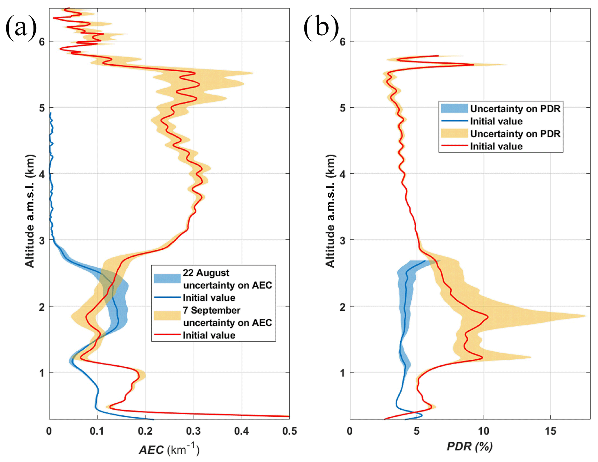
Figure A4Vertical profiles of the (a) AEC and (b) PDR at 355 nm on 22 August 2017 and 7 September 2017. The shaded areas give the uncertainty linked to the one on the LR of ± 25 sr as considered for the CALIOP operational algorithm.
PC inverted the ground-based and airborne lidar data, analysed the data and wrote the paper, with comments from all the co-authors; CF analysed the data and wrote the paper; JT aligned and validated the ground-based lidar; MG participated in the study of atmospheric dynamics and in the paper editing; GS participated in the back-trajectory computation; AB gathered the CATS lidar data and the wind fields; PF coordinated the AEROCLO-sA project; XL participated in the pre- and post-field calibration and operation of the lidar; KD and JFD maintained and operated the lidar during the field campaign.
The authors declare that they have no conflict of interest.
This article is part of the special issue “New observations and related modelling studies of the aerosol–cloud–climate system in the Southeast Atlantic and southern Africa regions (ACP/AMT inter-journal SI)”. It is not associated with a conference.
The authors would also like to thank the AERIS data centre for their support during the campaign and managing the AEROCLO-sA database. The research leading to these results has received funding from the European Union's Seventh Framework Programme (FP7/2014-2018) under EUFAR2 contract no. 312609. Airborne data were obtained using the aircraft managed by SAFIRE, the French facility for airborne research, an infrastructure of the French National Center for Scientific Research (CNRS), Météo-France and the French National Center for Space Studies (CNES). The authors would like to thank Frédéric Blouzon and Abdel Abchiche (DT-INSU) as well as Pascal Genau and Mathilde van Haecke (LATMOS) for their support in operating and processing the LNG data. The invaluable diplomatic assistance of the French Embassy in Namibia, the administrative support of the Service Partnership and Valorisation of the Regional Delegation of the Paris-Villejuif Region of the CNRS and the cooperation of the Namibian National Commission on Research, Science and Technology (NCRST) are sincerely acknowledged. The long-term hosting and support of the SANUMARC, a research centre of the University of Namibia in Henties Bay, have been essential through the years and are warmly appreciated. The authors acknowledge the MODIS science, processing and data support teams for producing and providing MODIS data (at https://modis.gsfc.nasa.gov/data/dataprod/, last access: 23 November 2019) and the NASA Langley Research Center Atmospheric Sciences Data Center for the data processing and distribution of CALIPSO products (level 4.10, at https://eosweb.larc.nasa.gov/HORDERBIN/HTML_Start.cgi, last access: 23 November 2019). The authors would like to thank the AERONET network for Sun photometer products (at https://aeronet.gsfc.nasa.gov/, last access: 23 November 2019). Finally, the authors are grateful to Michael Diamond and an anonymous reviewer for their comments that helped improve the overall quality of the paper.
This work was supported by the French National Research Agency under grant agreement no. ANR-15-CE01-0014-01, the French national programme LEFE/INSU, the Programme national de Télédetection Spatiale (PNTS; http://programmes.insu.cnrs.fr/pnts/, last access: 23 November 2019) grant no. PNTS-2016-14, the French National Agency for Space Studies (CNES) and the South African National Research Foundation (NRF) under grant UID 105958.
This paper was edited by Paquita Zuidema and reviewed by Michael Diamond and one anonymous referee.
Ackerman, A. S., Toon, O. B., Stevens, D. E., Heymsfield, A. J., Ramanathan, V., and Welton, E. J.: Reduction of tropical cloudiness by soot, Science, 288, 1042–1047, https://doi.org/10.1126/SCIENCE.288.5468.1042, 2000.
Adebiyi, A. A. and Zuidema, P.: The role of the southern African easterly jet in modifying the southeast Atlantic aerosol and cloud environments, Q. J. Roy. Meteorol. Soc., 142, 1574–1589, https://doi.org/10.1002/qj.2765, 2016.
Adebiyi, A. A., Zuidema, P., and Abel, S. J.: The convolution of dynamics and moisture with the presence of shortwave absorbing aerosols over the southeast Atlantic, J. Climate, 28, 1997–2024, https://doi.org/10.1175/JCLI-D-14-00352.1, 2015.
Andreae, M. O., Elbert, W., and de Mora, S. J.: Biogenic sulfur emissions and aerosols over the tropical South Atlantic: 3. Atmospheric dimethylsulfide, aerosols and cloud condensation nuclei, J. Geophys. Res., 100, 11335, https://doi.org/10.1029/94jd02828, 2004.
Ångström, A.: The parameters of atmospheric turbidity, Tellus A, 16, 64–75, https://doi.org/10.3402/tellusa.v16i1.8885, 1964.
Bates, T. S., Quinn, P. K., Coffman, D. J., Johnson, J. E., Miller, T. L., Covert, D. S., Wiedensohler, A., Leinert, S., Nowak, A., and Neusüss, C.: Regional physical and chemical properties of the marine boundary layer aerosol across the Atlantic during Aerosols99: An overview, J. Geophys. Res.-Atmos., 106, 20767–20782, https://doi.org/10.1029/2000JD900578, 2001.
Bruneau, D., Pelon, J., Blouzon, F., Spatazza, J., Genau, P., Buchholtz, G., Amarouche, N., Abchiche, A. and Aouji, O.: 355-nm high spectral resolution airborne lidar LNG: system description and first results, Appl. Opt., 54, 8776, https://doi.org/10.1364/AO.54.008776, 2015.
Burton, S. P., Ferrare, R. A., Hostetler, C. A., Hair, J. W., Rogers, R. R., Obland, M. D., Butler, C. F., Cook, A. L., Harper, D. B., and Froyd, K. D.: Aerosol classification using airborne High Spectral Resolution Lidar measurements – methodology and examples, Atmos. Meas. Tech., 5, 73–98, https://doi.org/10.5194/amt-5-73-2012, 2012.
Chazette, P.: The monsoon aerosol extinction properties at Goa during INDOEX as measured with lidar, J. Geophys. Res., 108, 4187, https://doi.org/10.1029/2002JD002074, 2003.
Chazette, P. and Totems, J.: Mini N2-Raman Lidar onboard ultra-light aircraft for aerosol measurements: Demonstration and extrapolation, Remote Sens., 2016, 9, https://doi.org/10.3390/rs9121226, 2017.
Chazette, P., Bocquet, M., Royer, P., Winiarek, V., Raut, J. C., Labazuy, P., Gouhier, M., Lardier, M., and Cariou, J. P.: Eyjafjallajökull ash concentrations derived from both lidar and modeling, J. Geophys. Res.-Atmos., 117, D00U14, https://doi.org/10.1029/2011JD015755, 2012a.
Chazette, P., Dabas, A., Sanak, J., Lardier, M., and Royer, P.: French airborne lidar measurements for Eyjafjallajökull ash plume survey, Atmos. Chem. Phys., 12, 7059–7072, https://doi.org/10.5194/acp-12-7059-2012, 2012b.
Chazette, P., Totems, J., Ancellet, G., Pelon, J., and Sicard, M.: Temporal consistency of lidar observations during aerosol transport events in the framework of the ChArMEx/ADRIMED campaign at Minorca in June 2013, Atmos. Chem. Phys., 16, 2863–2875, https://doi.org/10.5194/acp-16-2863-2016, 2016.
Chew, B. N., Campbell, J. R., Reid, J. S., Giles, D. M., Welton, E. J., Salinas, S. V., and Liew, S. C.: Tropical cirrus cloud contamination in sun photometer data, Atmos. Environ., 45, 6724–6731, https://doi.org/10.1016/j.atmosenv.2011.08.017, 2011.
Clements, C. B., Potter, B. E., and Zhong, S.: In situ measurements of water vapor, heat, and CO2 fluxes within a prescribed grass fire, Int. J. Wildl. Fire, 15, 299–306, https://doi.org/10.1071/WF05101, 2006.
Deaconu, L. T., Ferlay, N., Waquet, F., Peers, F., Thieuleux, F., and Goloub, P.: Satellite inference of water vapour and above-cloud aerosol combined effect on radiative budget and cloud-top processes in the southeastern Atlantic Ocean, Atmos. Chem. Phys., 19, 11613–11634, https://doi.org/10.5194/acp-19-11613-2019, 2019.
Dee, D. P., Uppala, S. M., Simmons, A. J., Berrisford, P., Poli, P., Kobayashi, S., Andrae, U., Balmaseda, M. A., Balsamo, G., Bauer, P., Bechtold, P., Beljaars, A. C. M., van de Berg, L., Bidlot, J., Bormann, N., Delsol, C., Dragani, R., Fuentes, M., Geer, A. J., Haimberger, L., Healy, S. B., Hersbach, H., Hólm, E. V, Isaksen, L., Kållberg, P., Köhler, M., Matricardi, M., Mcnally, A. P., Monge-Sanz, B. M., Morcrette, J. J., Park, B. K., Peubey, C., de Rosnay, P., Tavolato, C., Thépaut, J. N., and Vitart, F.: The ERA-Interim reanalysis: Configuration and performance of the data assimilation system, Q. J. Roy. Meteorol. Soc., 137, 553–597, 2011.
Diamond, M. S., Dobracki, A., Freitag, S., Small Griswold, J. D., Heikkila, A., Howell, S. G., Kacarab, M. E., Podolske, J. R., Saide, P. E., and Wood, R.: Time-dependent entrainment of smoke presents an observational challenge for assessing aerosol–cloud interactions over the southeast Atlantic Ocean, Atmos. Chem. Phys., 18, 14623–14636, https://doi.org/10.5194/acp-18-14623-2018, 2018.
Dieudonné, E., Chazette, P., Marnas, F., Totems, J., and Shang, X.: Raman Lidar Observations of Aerosol Optical Properties in 11 Cities from France to Siberia, Remote Sens., 9, 978, https://doi.org/10.3390/rs9100978, 2017.
Draxler, R. R. R. and Rolph, G. D. D.: HYSPLIT (HYbrid Single-Particle Lagrangian Integrated Trajectory) Model access via NOAA ARL READY Website (http://www.arl.noaa.gov/HYSPLIT.php, last access: 23 November 2019), NOAA Air Resources Laboratory, College Park, MD., NOAA Air Resour. Lab. available at: http://ready.arl.noaa.gov/HYSPLIT_ash.php (last access: 23 November 2019), 2014.
Dubovik, O., Smirnov, A., Holben, B. N., King, M. D., Kaufman, Y. J., Eck, T. F., and Slutsker, I.: Accuracy assessments of aerosol optical properties retrieved from Aerosol Robotic Network (AERONET) Sun and sky radiance measurements, J. Geophys. Res.-Atmos., 105, 9791–9806, https://doi.org/10.1029/2000JD900040, 2000.
Flamant, C., Pelon, J., Chazette, P., Trouillet, V., Quinn, P. K., Frouin, R., Bruneau, D., Leon, J.-F., Bates, T. S., Johnson, J., and Livingston, J.: Airborne lidar measurements of aerosol spatial distribution and optical properties over the Atlantic Ocean during a European pollution outbreak of ACE-2, Tellus B, 52, 662–677, doi:10.1034/j.1600-0889.2000.00083.x, 2000.
Formenti, P., Piketh, S. J., Namwoonde, A., Klopper, D., Burger, R., Cazaunau, M., Feron, A., Gaimoz, C., Broccardo, S., Walton, N., Desboeufs, K., Siour, G., Hanghome, M., Mafwila, S., Omoregie, E., Junkermann, W., and Maenhaut, W.: Three years of measurements of light-absorbing aerosols over coastal Namibia: seasonality, origin, and transport, Atmos. Chem. Phys., 18, 17003–17016, https://doi.org/10.5194/acp-18-17003-2018, 2018.
Formenti, P., D'Anna, B., Flamant, C., Mallet, M. D., Piketh, S. J., Schepanski, K., Waquet, F., Auriol, F., Brogniez, G., Burnet, F., Chaboureau, J.-P., Chauvigné, A., Chazette, P., Denjean, C., Desboeufs, K., Doussin, J.-F., Elguindi, N., Feuerstein, S., Gaetani, M., Giorio, C., Klopper, D., Mallet, M. D., Nabat, P., Monod, A., Solmon, F., Namwoonde, A., Chikwililwa, C., Mushi, R., Welton, E. J., Holben, B., Formenti, P., D'Anna, B., Flamant, C., Mallet, M. D., Piketh, S. J., Schepanski, K., Waquet, F., Auriol, F., Brogniez, G., Burnet, F., Chaboureau, J.-P., Chauvigné, A., Chazette, P., Denjean, C., Desboeufs, K., Doussin, J.-F., Elguindi, N., Feuerstein, S., Gaetani, M., Giorio, C., Klopper, D., Mallet, M. D., Nabat, P., Monod, A., Solmon, F., Namwoonde, A., Chikwililwa, C., Mushi, R., Welton, E. J. and Holben, B.: The Aerosols, Radiation and Clouds in southern Africa (AEROCLO-sA) field campaign in Namibia: overview, illustrative observations and way forward, B. Am. Meteor. Soc., 100, 1277–1298, https://doi.org/10.1175/BAMS-D-17-0278.1, 2019.
Fuchs, J., Cermak, J., Andersen, H., Hollmann, R., and Schwarz, K.: On the Influence of Air Mass Origin on Low-Cloud Properties in the Southeast Atlantic, J. Geophys. Res.-Atmos., 122, 11076–11091, https://doi.org/10.1002/2017JD027184, 2017.
Ginoux, P., Prospero, J. M., Gill, T. E., Hsu, N. C., and Zhao, M.: Global-scale attribution of anthropogenic and natural dust sources and their emission rates based on MODIS Deep Blue aerosol products, Rev. Geophys., 50, 1–36, https://doi.org/10.1029/2012RG000388, 2012.
Gordon, H., Field, P. R., Abel, S. J., Dalvi, M., Grosvenor, D. P., Hill, A. A., Johnson, B. T., Miltenberger, A. K., Yoshioka, M., and Carslaw, K. S.: Large simulated radiative effects of smoke in the south-east Atlantic, Atmos. Chem. Phys., 18, 15261–15289, https://doi.org/10.5194/acp-18-15261-2018, 2018.
Hamonou, E., Chazette, P., Balis, D., Dulac, F., Schneider, X., Galani, E., Ancellet, G., and Papayannis, A.: Characterization of the vertical structure of Saharan dust export to the Mediterranean basin, J. Geophys. Res., 104, 22257, https://doi.org/10.1029/1999JD900257, 1999.
Hoffmann, L., Günther, G., Li, D., Stein, O., Wu, X., Griessbach, S., Heng, Y., Konopka, P., Müller, R., Vogel, B., and Wright, J. S.: From ERA-Interim to ERA5: the considerable impact of ECMWF's next-generation reanalysis on Lagrangian transport simulations, Atmos. Chem. Phys., 19, 3097–3124, https://doi.org/10.5194/acp-19-3097-2019, 2019.
Holben, B. N., Eck, T. F., Slutsker, I., Tanré, D., Buis, J. P., Setzer, A., Vermote, E., Reagan, J. A., Kaufman, Y. J., Nakajima, T., Lavenu, F., Jankowiak, I., and Smirnov, A.: AERONET – A Federated Instrument Network and Data Archive for Aerosol Characterization, Remote Sens. Environ., 66, 1–16, https://doi.org/10.1016/S0034-4257(98)00031-5, 1998.
Holz, A., Paritsis, J., Mundo, I. A., Veblen, T. T., Kitzberger, T., Williamson, G. J., Aráoz, E., Bustos-Schindler, C., González, M. E., Grau, H. R., and Quezada, J. M.: Southern Annular Mode drives multicentury wildfire activity in southern South America., P. Natl. Acad. Sci. USA, 114, 9552–9557, https://doi.org/10.1073/pnas.1705168114, 2017.
Ichoku, C., Giglio, L., Wooster, M. J., and Remer, L. A.: Global characterization of biomass-burning patterns using satellite measurements of fire radiative energy, Remote Sens. Environ., 112, 2950–2962, https://doi.org/10.1016/j.rse.2008.02.009, 2008.
Johansson, L., Jalkanen, J. P., and Kukkonen, J.: Global assessment of shipping emissions in 2015 on a high spatial and temporal resolution, Atmos. Environ., 167, 403–415, https://doi.org/10.1016/j.atmosenv.2017.08.042, 2017.
Jones, A. and Haywood, J. M.: Sea-spray geoengineering in the HadGEM2-ES earth-system model: radiative impact and climate response, Atmos. Chem. Phys., 12, 10887–10898, https://doi.org/10.5194/acp-12-10887-2012, 2012.
Jones, A., Haywood, J., and Boucher, O.: Climate impacts of geoengineering marine stratocumulus clouds, J. Geophys. Res.-Atmos., 114, D10106, https://doi.org/10.1029/2008JD011450, 2009.
Keil, A. and Haywood, J. M.: Solar radiative forcing by biomass burning aerosol particles during SAFARI 2000: A case study based on measured aerosol and cloud properties, J. Geophys. Res.-Atmos., 108, 8467–8476, https://doi.org/10.1029/2002jd002315, 2003.
Kim, M.-H., Omar, A. H., Tackett, J. L., Vaughan, M. A., Winker, D. M., Trepte, C. R., Hu, Y., Liu, Z., Poole, L. R., Pitts, M. C., Kar, J., and Magill, B. E.: The CALIPSO version 4 automated aerosol classification and lidar ratio selection algorithm, Atmos. Meas. Tech., 11, 6107–6135, https://doi.org/10.5194/amt-11-6107-2018, 2018.
Kim, S.-W., Chazette, P., Dulac, F., Sanak, J., Johnson, B., and Yoon, S.-C.: Vertical structure of aerosols and water vapor over West Africa during the African monsoon dry season, Atmos. Chem. Phys., 9, 8017–8038, https://doi.org/10.5194/acp-9-8017-2009, 2009.
King, M. D., Kaufman, Y. J., Menzel, W. P., and Tanré, D.: Remote Sensing of Cloud, Aerosol, and Water Vapor Properties from the Moderate Resolution Imaging Spectrometer (MODIS), IEEE T. Geosci. Remote, 30, 2–27, https://doi.org/10.1109/36.124212, 1992.
Léon, J.-F., Chazette, P., Pelon, J., Dulac, F., Randriamiarisoa, H., patrick Chazette, Pelon, J., Dulac, F., and Randriamiarisoa, H.: Aerosol direct radiative impact over the INDOEX area based on passive and active remote sensing, J. Geophys. Res., 107, 8006, https://doi.org/10.1029/2000JD000116, 2002.
Lim, E.-P., Hendon, H. H., Arblaster, J. M., Delage, F., Nguyen, H., Min, S.-K., and Wheeler, M. C.: The impact of the Southern Annular Mode on future changes in Southern Hemisphere rainfall, Geophys. Res. Lett., 43, 7160–7167, https://doi.org/10.1002/2016GL069453, 2016.
McFarquhar, G. M. and Wang, H.: Effects of aerosols on trade wind cumuli over the Indian Ocean: Model simulations, Q. J. Roy. Meteorol. Soc., 132, 821–843, https://doi.org/10.1256/qj.04.179, 2006.
Müller, D., Ansmann, A., Mattis, I., Tesche, M., Wandinger, U., Althausen, D., and Pisani, G.: Aerosol-type-dependent lidar ratios observed with Raman lidar, J. Geophys. Res., 112, D16202, https://doi.org/10.1029/2006JD008292, 2007.
Myhre, G., Samset, B. H., Schulz, M., Balkanski, Y., Bauer, S., Berntsen, T. K., Bian, H., Bellouin, N., Chin, M., Diehl, T., Easter, R. C., Feichter, J., Ghan, S. J., Hauglustaine, D., Iversen, T., Kinne, S., Kirkevåg, A., Lamarque, J.-F., Lin, G., Liu, X., Lund, M. T., Luo, G., Ma, X., van Noije, T., Penner, J. E., Rasch, P. J., Ruiz, A., Seland, Ø., Skeie, R. B., Stier, P., Takemura, T., Tsigaridis, K., Wang, P., Wang, Z., Xu, L., Yu, H., Yu, F., Yoon, J.-H., Zhang, K., Zhang, H., and Zhou, C.: Radiative forcing of the direct aerosol effect from AeroCom Phase II simulations, Atmos. Chem. Phys., 13, 1853–1877, https://doi.org/10.5194/acp-13-1853-2013, 2013.
Nicolet, M.: On the molecular scattering in the terrestrial atmosphere?: An empirical formula for its calculation in the homosphere, Planet. Space Sci., 32, 1467–1468, https://doi.org/10.1016/0032-0633(84)90089-8, 1984.
Oreopoulos, L. and Platnick, S.: Radiative susceptibility of cloudy atmospheres to droplet number perturbations: 2. Global analysis from MODIS, J. Geophys. Res., 113, D14S21, https://doi.org/10.1029/2007JD009655, 2008.
Parmar, R. S., Welling, M., Andreae, M. O., and Helas, G.: Water vapor release from biomass combustion, Atmos. Chem. Phys., 8, 6147–6153, https://doi.org/10.5194/acp-8-6147-2008, 2008.
Ramanathan, V., Li, F., Ramana, M. V, Praveen, P. S., Kim, D., Corrigan, C. E., Nguyen, H., Stone, E. A., Schauer, J. J., Carmichael, G. R., Adhikary, B., and Yoon, S. C.: Atmospheric brown clouds: Hemispherical and regional variations in long-range transport, absorption, and radiative forcing, J. Geophys. Res, 112, 22–21, https://doi.org/10.1029/2006JD008124, 2007.
Raut, J.-C. and Chazette, P.: Radiative budget in the presence of multi-layered aerosol structures in the framework of AMMA SOP-0, Atmos. Chem. Phys., 8, 6839–6864, https://doi.org/10.5194/acp-8-6839-2008, 2008.
Raut, J.-C. and Chazette, P.: Assessment of vertically-resolved PM10 from mobile lidar observations, Atmos. Chem. Phys., 9, 8617–8638, https://doi.org/10.5194/acp-9-8617-2009, 2009.
Remer, L. A., Kaufman, Y. J., Tanré, D., Mattoo, S., Chu, D. A., Martins, J. V., Li, R.-R., Ichoku, C., Levy, R. C., Kleidman, R. G., Eck, T. F., Vermote, E., and Holben, B. N.: The MODIS Aerosol Algorithm, Products, and Validation, J. Atmos. Sci., 62, 947–973, https://doi.org/10.1175/JAS3385.1, 2005.
Royer, P., Raut, J.-C., Ajello, G., Berthier, S., and Chazette, P.: Synergy between CALIOP and MODIS instruments for aerosol monitoring: application to the Po Valley, Atmos. Meas. Tech., 3, 893–907, https://doi.org/10.5194/amt-3-893-2010, 2010.
Royer, P., Chazette, P., Lardier, M. and Sauvage, L.: Aerosol content survey by mini Raman lidar: Application to local and long-range transport aerosols, Atmos. Environ., 45, 7487–7495, https://doi.org/10.1016/j.atmosenv.2010.11.001, 2011a.
Royer, P., Chazette, P., Lardier, M. and Sauvage, L.: Aerosol content survey by mini N2-Raman lidar: Application to local and long-range transport aerosols, Atmos. Environ., 45, 7487–7495, https://doi.org/10.1016/j.atmosenv.2010.11.001, 2011b.
Salmonson, V. V., Barnes, W. L., Maymon, P. W., Montgomery, H. E., and Ostrow, H.: MODIS: Advanced Facility Instrument for Studies of the Earth as a System, IEEE T. Geosci. Remote, 27, 145–153, https://doi.org/10.1109/36.20292, 1989.
Stein, A. F., Draxler, R. R., Rolph, G. D., Stunder, B. J. B., Cohen, M. D., Ngan, F., Stein, A. F., Draxler, R. R., Rolph, G. D., Stunder, B. J. B., Cohen, M. D., and Ngan, F.: NOAA's HYSPLIT Atmospheric Transport and Dispersion Modeling System, B. Am. Meteor. Soc., 96, 2059–2077, https://doi.org/10.1175/BAMS-D-14-00110.1, 2015.
Stier, P., Schutgens, N. A. J., Bellouin, N., Bian, H., Boucher, O., Chin, M., Ghan, S., Huneeus, N., Kinne, S., Lin, G., Ma, X., Myhre, G., Penner, J. E., Randles, C. A., Samset, B., Schulz, M., Takemura, T., Yu, F., Yu, H., and Zhou, C.: Host model uncertainties in aerosol radiative forcing estimates: results from the AeroCom Prescribed intercomparison study, Atmos. Chem. Phys., 13, 3245–3270, https://doi.org/10.5194/acp-13-3245-2013, 2013.
Stohl, A.: Computation, accuracy and applications of trajectories – A review and bibliography, Atmos. Environ., 32, 947–966, https://doi.org/10.1016/S1352-2310(97)00457-3, 1998.
Swap, R. J., Annegarn, H. J., Suttles, J. T., King, M. D., Platnick, S., Privette, J. L., and Scholes, R. J.: Africa burning: A thematic analysis of the Southern African Regional Science Initiative (SAFARI 2000), J. Geophys. Res.-Atmos., 108, 8465–8479, https://doi.org/10.1029/2003JD003747, 2003.
Trenberth, K. E.: Interannual Variability of the 500 mb Zonal Mean Flow in the Southern Hemisphere, Mon. Weather Rev., 107, 1515–1524, https://doi.org/10.1175/1520-0493(1979)107<1515:ivotmz>2.0.co;2, 2002.
Tyson, P. D. and Preston-White, R. A.: The weather and climate of southern Africa, Oxford University Press, available at: https://global.oup.com/academic/product/the-weather-and-climate-of-southern-africa-9780195718065?lang=en&cc=in (last access: 29 April 2019), 2000.
Vickery, K. J., Eckardt, F. D., and Bryant, R. G.: A sub-basin scale dust plume source frequency inventory for southern Africa, 2005–2008, Geophys. Res. Lett., 40, 5274–5279, https://doi.org/10.1002/grl.50968, 2013.
Winker, D. M., Hunt, W. H., and McGill, M. J.: Initial performance assessment of CALIOP, Geophys. Res. Lett., 34, L19803, https://doi.org/10.1029/2007GL030135, 2007.
Yorks, J. E., McGill, M. J., Palm, S. P., Hlavka, D. L., Selmer, P. A., Nowottnick, E. P., Vaughan, M. A., Rodier, S. D., and Hart, W. D.: An overview of the CATS level 1 processing algorithms and data products, Geophys. Res. Lett., 43, 4632–4639, https://doi.org/10.1002/2016GL068006, 2016.
Zuidema, P., Redemann, J., Haywood, J., Wood, R., Piketh, S., Hipondoka, M., and Formenti, P.: Smoke and clouds above the southeast Atlantic: Upcoming field campaigns probe absorbing aerosol's impact on climate, B. Am. Meteor. Soc., 97, 1131–1135, https://doi.org/10.1175/BAMS-D-15-00082.1, 2016.
Zuidema, P., Sedlacek, A. J., Flynn, C., Springston, S., Delgadillo, R., Zhang, J., Aiken, A. C., Koontz, A., and Muradyan, P.: The Ascension Island Boundary Layer in the Remote Southeast Atlantic is Often Smoky, Geophys. Res. Lett., 45, 4456–4465, https://doi.org/10.1002/2017GL076926, 2018.
- Abstract
- Introduction
- Observations and simulations
- Temporal evolution of the aerosol properties and vertical distribution over Henties Bay
- Vertical distribution from airborne observations
- Origin of elevated BBA layers over Henties Bay
- Conclusions
- Data availability
- Appendix A: Ground-based lidar analysis – link with space-borne lidar observations
- Author contributions
- Competing interests
- Special issue statement
- Acknowledgements
- Financial support
- Review statement
- References