the Creative Commons Attribution 4.0 License.
the Creative Commons Attribution 4.0 License.
 | 10 Dec 2019
The impact of fluctuations and correlations in droplet growth by collision–coalescence revisited – Part 2: Observational evidence of gel formation in warm clouds
Lester Alfonso
Graciela B. Raga
Darrel Baumgardner
In recent papers (Alfonso et al., 2013; Alfonso and Raga, 2017) the sol–gel transition was proposed as a mechanism for the formation of large droplets required to trigger warm rain development in cumulus clouds. In the context of cloud physics, gelation can be interpreted as the formation of the “lucky droplet” that grows by accretion of smaller droplets at a much faster rate than the rest of the population and becomes the embryo for raindrops. However, all the results in this area have been theoretical or simulation studies. The aim of this paper is to find some observational evidence of gel formation in clouds by analyzing the distribution of the largest droplet at an early stage of cloud formation and to show that the mass of the gel (largest drop) is a mixture of a Gaussian distribution and a Gumbel distribution, in accordance with the pseudo-critical clustering scenario described in Gruyer et al. (2013) for nuclear multi-fragmentation.
- Article
(3553 KB) - Companion paper
- BibTeX
- EndNote


A fundamental, ongoing problem in cloud physics is associated with the discrepancy between the times modeled and observed for the formation of precipitation in warm clouds. Observational studies show that precipitation can develop in less than 20 min. For example, in Göke et al. (2007), an analysis of radar observations in the framework of the Small Cumulus Microphysics Study (SCMS), demonstrated that maritime clouds increased their reflectivity from −5 to +7.5 dBZ in a characteristic time of 333 s. Simulations of the collision and coalescence process, such as those described in the review published by Beard and Ochs (1993), require longer times for precipitation formation, unless giant nuclei (aerosols with diameters greater than 2 µm) are incorporated in the simulation.
Numerous mechanisms have been proposed to close the gap between observations and simulations. Some theories explain this phenomenon as an increase in collision efficiencies due to turbulence (Wang et al., 2008; Pinsky and Khain, 2004; Pinsky et al., 2007, 2008), turbulence-enhanced collision rate of cloud droplets (Falkovich and Pumir, 2007; Grabowski and Wang, 2013) or turbulent dispersion of cloud droplets (Sidin et al., 2009).
More recent papers (Onishi and Seifert, 2016; Li et al., 2017, 2018, and Chen et al., 2018) also investigated the effect of turbulence in early development of precipitation.
Other research points to the supersaturation fluctuations resulting from homogeneous (Warner, 1969) and inhomogeneous mixing (Baker et al., 1980), which allow some droplets to grow faster by condensation in areas with larger supersaturation. Cooper (1989) found evidence of faster growth of the larger droplets due to the variability that results from mixing and random positioning of droplets during cloud formation. Shaw et al. (1998) explored the possibility that vortex structures in a turbulent cloud cause variations in droplet concentration and supersaturation (at the centimeter scale), allowing droplets in areas of higher concentration to grow more rapidly. Their calculations show an important widening of the spectrum from this mechanism. Roach (1976) showed that the growth of larger droplets increases due to radiative cooling at the top of stratiform clouds and the addition of sulfate cloud condensation nuclei (CCN), activated as droplets as a result of aqueous-phase chemical reactions (Zhang et al., 1999). In the same manner, Feingold and Chuang (2002) proposed the theory that certain organic compounds (film-forming compounds) can create a layer around droplets that inhibits their growth, causing a fraction of droplets to grow under conditions of higher supersaturation with the consequent widening of the spectrum. The existence of giant CCN is another of the proposed mechanisms. Even at concentrations as low as 1 L−1, they can contribute significantly to the broadening of the spectrum (Johnson, 1982; Feingold et al., 1999; Yin et al., 2000; Van Den Heever and Cotton, 2007).
More recently, the sol–gel transition has been proposed as a possible mechanism for the formation of embryonic drops that trigger the formation of precipitation (Alfonso et al., 2010, 2013). Although this phenomenon is not as well known in the field of cloud physics, the sol–gel transition (also known as “gelation” in English-language literature), has been widely studied in other fields of research to explain, for example, the formation of planets (Wetherill, 1990) and aerogels in aerosol physics (Lushnikov, 1978) or the emergence of giant components in percolation theory (Aldous, 1999).
In the framework of cloud physics, the sol–gel phenomenon can be interpreted as the formation of the lucky droplet that becomes the embryo for raindrops and is defined by a transition from a continuous system of small droplets, to another system with a continuous spectrum plus a giant drop (runaway droplet, embryonic drop, gel) that interacts with the system increasing its mass by accretion with the smallest drops.
Telford (1955) may be the first to propose the “lucky droplet” model for collision–coalescence of cloud droplets. One of the novelties of Telford's approach was to recognize the shortcomings of the “continuous growth model” and took into account the statistical fluctuations inherent to the collision–coalescence process and its discrete nature. He performed his analysis for a cloud consisting of identical 10 µm droplets together with collector drops with twice the volume (12.6 µm radius). From this initial bimodal distribution, he found that 100 of the 12.6 µm droplets per cubic meter (a 10−6 fraction), will grow more rapidly than predicted by the continuous growth model, experiencing their first 10 coalescences after a time of approximately 5 min, while the time to undergo 10 collisions assuming continuous growth was about 33 min.
The lucky droplet model was further developed by Kostinski and Shaw (2005), who presented numerical evidence that their model can lead to a rapid development of precipitation. Their analysis was based on the derivation of the distribution of times for N collisions (which gave the result of an Erlang distribution). They concluded that the 10−6 lucky droplets are expected to reach 50 µm 10 times faster than the average droplet. More recently, Wilkinson (2016) further advanced the model by using large deviation theory (Touchette, 2009). He derived the probability for the time T to undergo N collisions being a very small fraction of its mean value and showed that the timescale for the initiation of precipitation is smaller than the mean time for a single collision.
The results obtained by Kostinski and Shaw (2005) were tested by Dziekan and Pawlowska (2017) by calculating the “luck factor”, i.e., how much faster the luckiest droplets grow to r=40 µm compared to the average droplets. They estimated that the luckiest 10−3 fraction will cross the size gap around 5 times faster, and the luckiest 10−5 fraction was around 11 times faster, in good agreement with the results obtained by Kostinksi and Shaw (2005) (about 6 and 9 times faster, respectively).
However, previous efforts in this direction were mainly focused on finding the distribution of times for N collisions (Telford, 1955; Kostinski and Shaw, 2005; Wilkinson, 2016), while we were concentrated on studying the lucky droplet size distribution to determine whether or not the runaway growth process due to collision–coalescence has started.
Recent studies that address the sol–gel transition interpretation in cloud physics (Alfonso et al., 2013; Alfonso and Raga, 2017) analyze the problem from the theoretical and simulation point of view. The aim of the present work here is to find observational evidence of gel formation, taking as a reference recent studies in percolation theory (Botet and Płoszajczak, 2005) and nuclear physics (Botet et al., 2001; Gruyer et al., 2013), which can shed some light on the gel (largest droplet) size distribution during the initial stage of precipitation formation.
The paper is organized as follows: Sect. 2 presents an overview of previous results for both infinite and finite systems. An analysis of the largest droplet distribution from synthetic data obtained from Monte Carlo simulations (for the product and hydrodynamic kernels, respectively) is presented in Sect. 3. Sect. 4 is devoted to the analysis of experimental data. Finally, in Sect. 5 we discuss our results accompanied by the relevant conclusions.
2.1 Results for infinite systems in coagulation and percolation theory
The most commonly accepted approach to modeling the collision coalescence process in cloud models with detailed microphysics relies upon the Smoluchowski kinetic equation or kinetic collection equation (KCE), governing the time evolution of the average number of particles. The discrete form of this equation can be written as follows (Pruppacher and Klett, 1997):
where N(i,t) is the average concentration of droplets with mass xi at time t, and K(i,j) is the coagulation kernel related to the probability of coalescence of two drops of masses xi and xj. In Eq. (1), the first term on the right-hand side describes the average rate of production of droplets of mass xi due to coalescence between pairs of drops, whose masses add up to mass xi, and the second term describes the average rate of depletion of droplets with mass xi due to their collision and coalescence with other droplets.
However, the KCE may have a serious limitation in some cases (Lushnikov, 2004) and hence cannot accurately describe the coagulation process. The limitation essentially lies in the fact that the coagulation equation inevitably creates particles with infinite mass. For example, for a multiplicative coagulation kernel (), an attempt to calculate the second moment of the droplet mass spectrum:
leads to the result
Thus, after t=Tgel, the second moment may become undefined, and the total mass of the system starts to decrease (see Appendix A for more details). This result applies to infinite (with negligible fluctuations and correlations) coagulating systems in the thermodynamic limit, which is the limit for a large number K of particles where the volume V is taken to grow in proportion with the number of particles. Then, in the limit . The infinite system interpretation of the sol–gel transition assumes the presence of a gel phase (which is not predicted by the KCE equation) and introduces an additional assumption as to whether or not the gel interacts with the infinite size clusters that are not described by the KCE equation.
The other scenario considers that coagulation takes place in a system with a finite number of monomers in a finite volume. This approach is based on the scheme developed by Markus (1968) and Bayewitz et al. (1974) and was studied by Lushnikov (1978, 2004), Tanaka and Nakazawa (1993, 1994), and Matsoukas (2015) by using analytical tools and more recently by Alfonso (2015) and Alfonso and Raga (2017) numerically. Within this approach there is no mass loss, and the phase transition is manifested in the emergence of a giant particle that contains a finite fraction of the total mass of the system. Solutions in the post-gel regime were obtained analytically by Lushnikov (2004) and Matsoukas (2015) and numerically by Alfonso and Raga (2017).
The sol–gel transition has been observed experimentally. For example, aerogels in aerosol physics (Lushnikov et al., 1990) and in other theoretical models, such as that of percolation (Botet and Płoszajczak, 2005; Kolb and Axelos, 1990), where there is a close analogy between percolation and droplet coagulation. In bond percolation, each lattice corresponds to a monomer, and a proportion p of active bonds is set randomly between sites. Then clusters of size s are defined as an ensemble of s-occupied sites connected by active bonds. For a definite value of p=pc, a macroscopic cluster appears, corresponding to the sol–gel transition.
Recent results in percolation theory show that the largest cluster follows the Gumbel distribution for subcritical percolation (Bazant, 2000) and, at the critical point, follows the Kolmogorov–Smirnov (K-S) distribution (Botet and Płoszajczak, 2005). The K-S distribution is the distribution of the maximum value of the deviation between the experimental realization of a random process and its theoretical cumulative distribution, and it has following the cumulative distribution:
or the equivalent expression:
Botet and Płoszajczak (2005) also found evidence (from numerical solutions of the KCE equation) that, for multiplicative coalescence (with a collection kernel proportional to the product of the masses), the largest cluster follows the distribution in Eqs. (5a) and (5b) at the time of the phase transition. At this point, a hypothesis is formed in which the results obtained in percolation are extrapolated in order to find the probability distribution of the largest (runaway) droplet at t=Tgel.
2.2 Some theoretical and experimental results for finite systems in coagulation theory and nuclear physics
We will now consider some results obtained for finite systems in coagulation theory (Botet, 2011) and in nuclear physics (Gruyer et al., 2013). Unlike those in infinite systems, fluctuations and correlations in a finite system are not negligible.
We must emphasize that phase transitions cannot take place in a finite system. This is due to the fact that a phase transition is defined as a singularity in the free energy or any thermodynamic property of a system. For finite-sized systems, the free energy is proportional to the logarithm of a finite number of exponentials, which are always positive (Bhattacharjee, 2001). Consequently, those singularities are only possible within infinite systems by taking the thermodynamic limit. Thus, for finite systems, the notion of pseudo-critical region is introduced (which is the finite system equivalent of a sol–gel transition time).
Some interesting simulation and experimental results were obtained for these systems in Botet (2011) for the Smoluchowski model (1) and in Gruyer et al. (2013) for nuclear multi-fragmentation. Botet et al. (2001) found, from stochastic simulations of coagulation process with the product kernel (for a system of N=512 monomers), that the distribution of the largest cluster in the pseudo-critical region can be described as a mixture of the well-known Gaussian and Gumbel distributions:
In Eq. (6), the coefficients θ and (1−θ) are the mixture weights (probabilities associated with each component). The individual distributions and are the mixture components.
The Gumbel distribution is one of the asymptotic distributions from extreme value theory (EVT) and has the following form:
where μ is the position parameter and β the scale parameter. The distribution in Eq. (6) has its origin in the fact that, for finite systems in the pseudo-critical zone, the system experiences large fluctuations and the gel distribution is a combination of both distributions, a Gumbel and a Gaussian (Gruyer et al., 2013). A similar result was obtained by Botet (2011) using synthetic data from stochastic simulations, for collision probabilities proportional to the product of the masses.
The fundamental hypothesis of our work is that the gel mass (largest drop) in the initial phase of precipitation formation is distributed as a mixture of two asymptotic distributions: one Gumbel and one Gaussian, following the pseudo-critical clustering scenario described in Gruyer et al. (2013).
3.1 Results for the product kernel ()
For synthetic data analysis, the empirical distributions of the largest droplet mass (Mmax) were obtained from Monte Carlo simulations, following Botet (2011). The species-accounting formulation (Laurenzi et al., 2002) of the stochastic simulation algorithm (SSA) of Gillespie (1975), which rigorously accounts for fluctuations and correlations in a coalescing system, was used for the stochastic simulation in this work (see Appendix B).
The main difference between the Gillespie's SSA and other Monte Carlo methods based on the simulation particles (SIPs) approach (like the super droplet method developed by Shima et al., 2009) is that the Gillespie's SSA involved the collision of only two physical particles (droplets in our case) per MC cycle, while the approach based on SIP in each MC cycle collides SIP (super droplets, for example), which represents multiple numbers of droplets with the same attributes (radius r or mass in the simplest case) and position. However, Gillespie's SSA works perfectly for our purposes because, due to the finiteness of our systems, our simulations are performed for small volumes with a small number of droplets (in the range 50–300 cm−3).
Our methodology of synthetic data analysis consists of generating N-realizations (at each time step) using the algorithm of Gillespie. For each realization, there is a certain distribution of droplets. The largest droplet mass obtained from each distribution at each realization (for a fixed time step) would be the distribution to be fitted to the distribution in Eq. (6). Thus, the sample size would be equal to the number of realizations of the Monte Carlo algorithm.
Simulations were performed for the product kernel (), with an initial mono-disperse distribution of 100 droplets of 14 µm in radius (droplet mass g) in a cloud volume of 1 cm3, with cm3 s−1.
The product kernel is proportional to the product of the masses of the colliding droplets. It is widely used because analytical solutions of the KCE or Smoluchowski equation (Eq. 1) have been obtained for this kernel by Golovin (1963), Scott (1968), Drake (1972), and Drake and Wright (1972). The value of the constant C ( cm3 g−2 s−1) in the product kernel is the result of the polynomial approximation (Long, 1974) of the hydrodynamic collection kernel (Eq. 11).
The empirical distribution of the maxima was obtained for 1000 realizations of the stochastic algorithm. There is no need for a larger number of realizations to get better statistics, since the number of realizations in our Monte Carlo algorithm must be equal to the sample size in the application of the block maxima (BM) approach (see the next section for more details). On the other hand, this number is not much bigger than the number of blocks in the data for which the largest droplet maxima was fitted to fog data.
Figure 1a–d present the largest droplet mass empirical distributions obtained at four different times. Note that Eq. (6) provides a good fit for the distribution of the mass of the largest droplet (Mmax) both around and far from the sol–gel transition time (Tgel), which was calculated from Eq. (4) and found to be equal to 1378 s.
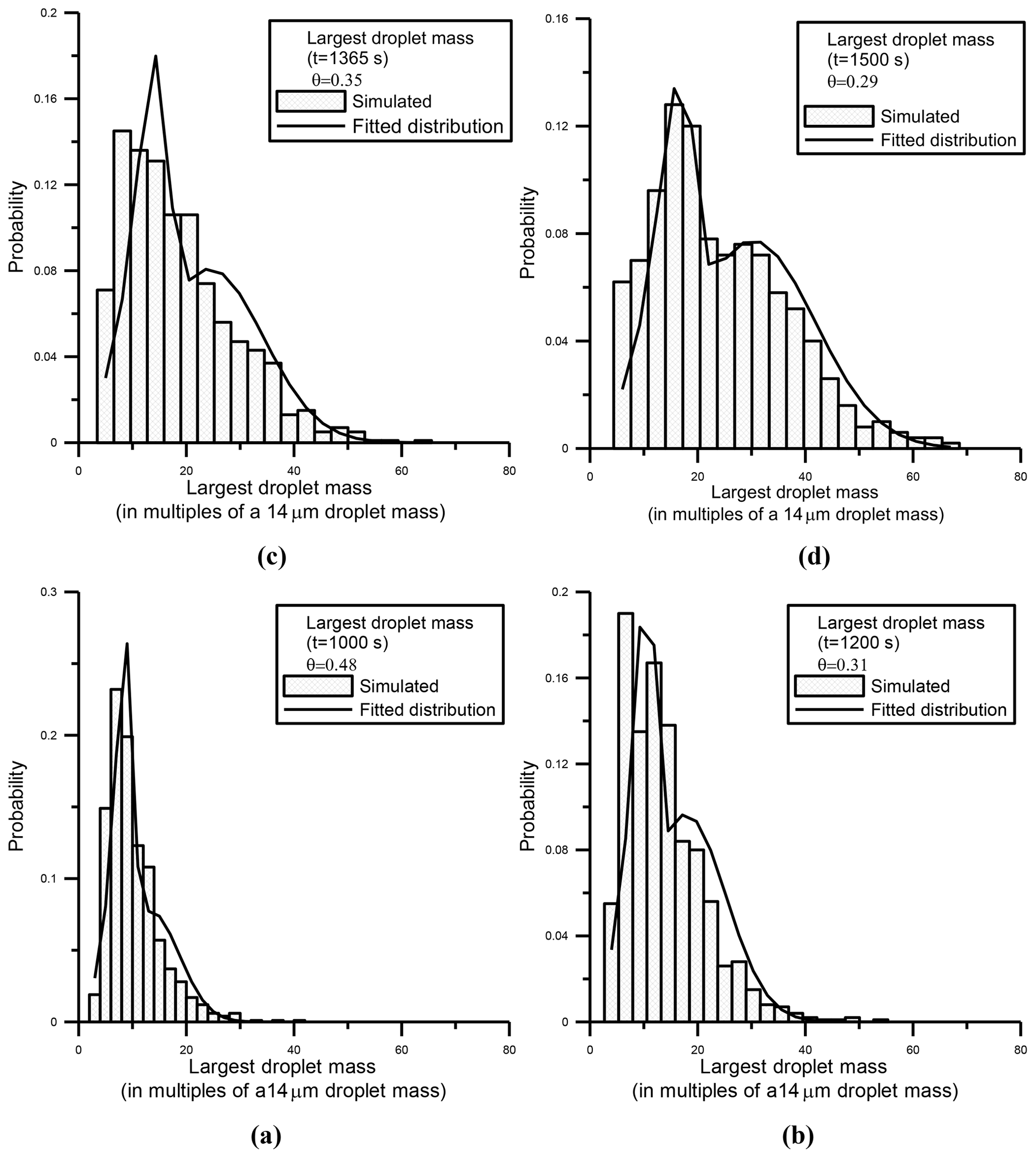
Figure 1Panels (a)–(d) (histograms) show the largest droplet mass distributions calculated from Monte Carlo simulations at four different times, for a system with an initial mono-disperse distribution of 100 droplets of 14 µm in radius. The solid line shows the fit using Eq. (6).
Figure 2 presents the time evolution of the coefficient θ, which represents the mixing fraction in Eq. (6) for the time interval [500 s, 2000 s]. Despite the noisy behavior of the coefficient θ (due to the finiteness of the system), there is a decreasing trend with time, showing larger values of θ (∼0.65) for times close to 500 s and values down to 0.2 at the end of the time interval. This figure indicates that, although the largest droplet distribution is adequately described by a mixture of Gaussian and Gumbel distributions, it has a larger Gumbel component (see Eq. 6) during the early stages of the coagulation process. As time progresses, the Gaussian contribution becomes more important (smaller values of θ) in providing a better fit to the largest droplet mass distribution.

Figure 2Time evolution of the coefficient θ in Eq. (6), obtained for a simulation with the product kernel.
These findings are in accordance with Gruyer et al. (2013) and Botet (2011): at an early stage of coagulation development, correlations are negligible, and, consequently, the largest fragments can be considered independent random variables. Therefore, the probability distribution of the largest fragment is given by the limit theorem for extremal variables, which states that the maximum of sample-independent and identically distributed random variables can only converge in distribution in the form of one of three possible distributions: Gumbel, Fréchet or Weibull.
As the coagulation process continues, fluctuations and correlations between droplets increase and the system reaches a critical point (Alfonso and Raga, 2017). Where the largest droplets are no longer independent random variables, the limit theorem for extremal variables no longer applies, and the largest droplet distribution is no longer described by a Gumbel distribution. At later times, away from the pseudo-critical region, the Gaussian contribution is the most important part of the largest droplet mass distribution. This can be explained by the additive nature of the process at this stage (Botet, 2011; Gruyer et al., 2013; Clusel and Bertoin, 2008), and the central limit theorem applies.
In the intermediate zone (which can be defined as the pseudo-critical zone), the distribution is well described by a mixture of Gumbel and Gaussian distributions and the weights associated with each distribution are comparable. It is expected that it can be observed that θ=0.5 at the infinite system critical point, Tgel, found to be 1378 s from Eq. (4). However, due to the finiteness of the system, the critical point corresponds approximately to a value θ=0.35 (see Fig. 2).
We can find whether or not a system is in the pseudo-critical region by defining the following ratio (Botet, 2011; Gruyer et al., 2013):
where wGumbel=θ and are the relative weights of the Gumbel and Gaussian distributions, respectively (see Eq. 6). By definition, corresponds to pure Gaussian and Gumbel distributions. If , the system is in the pseudo-critical domain.
Alternatively, Botet (2011) estimates the limits of the pseudo-critical region as the times when the largest droplet mass standard deviation σ(Mmax) calculated from Eq. (9) is small.
In Eq. (9), Nr is the number of iterations of the stochastic simulation algorithm of Gillespie (1975), Mmax the mass of the largest particle and 〈Mmax〉 its ensemble mean over all the realizations.
Even though the second moment of the distribution M2(τ) diverges (see Eq. 3) for the infinite system, there is no divergence of the second moment for a finite system (with no critical behavior). For that case, the standard deviation for the largest particle mass (σ(Mmax)) is expected to reach a maximum in the vicinity of . Moreover, computing the time evolution of the normalized standard deviation instead of σ(Mmax) yielded better results in estimating Tgel in Inaba et al. (1999), Alfonso et al. (2008, 2010, 2013), and Alfonso and Raga (2017).
Figure 3a shows the time evolution of , as an example for the system defined at the beginning of this section. Note that the maximum occurs at T=1315 s, close to Tgel=1378 s calculated from Eq. (4), and the time when the maximum of occurs is a reliable estimate of the sol–gel transition time for the corresponding infinite system.
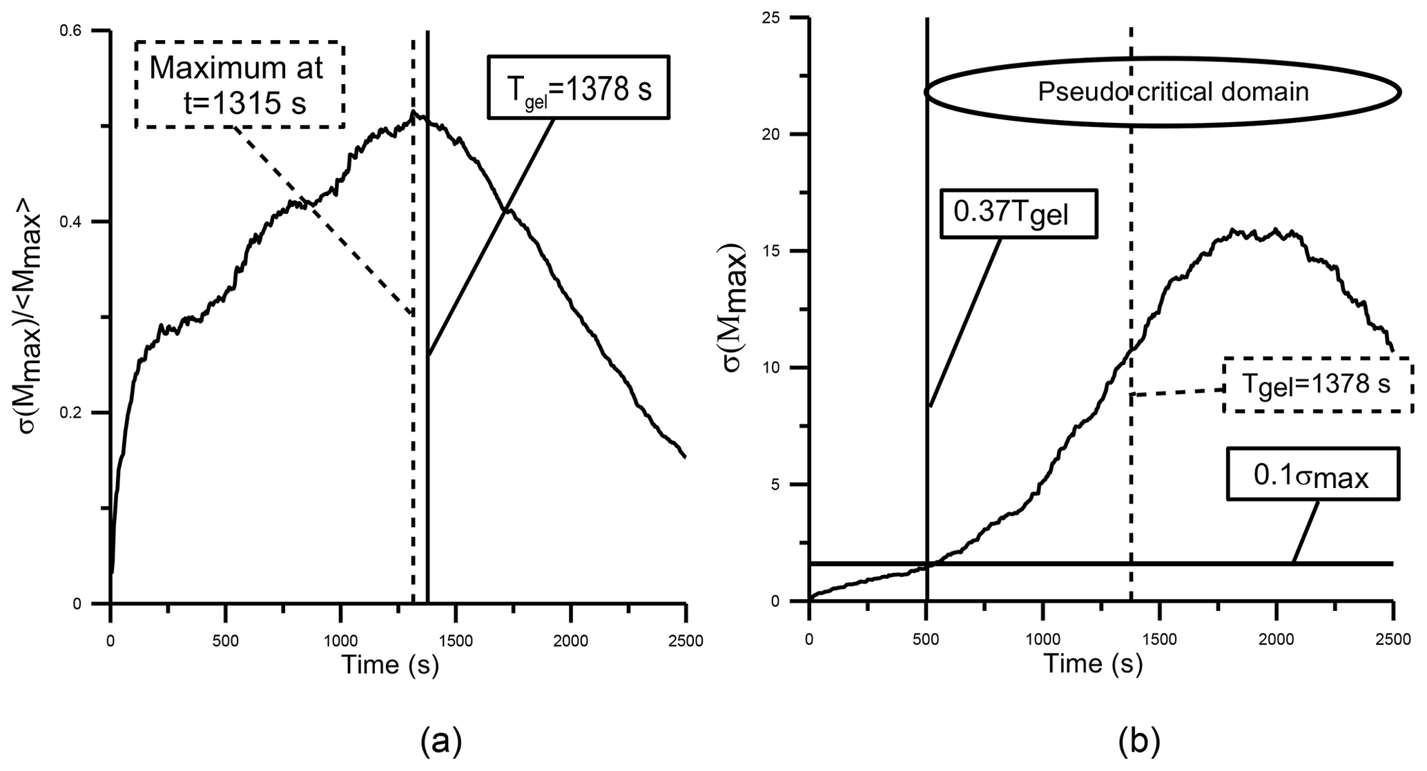
Figure 3For the finite system, the normalized standard deviation of the largest droplet mass versus time (a). The initial number of droplets was set equal to N=100 droplets of 14 µm in radius in a volume of 1 cm3. Simulations were performed with the product kernel (with cm3 g−2 s−1), and Nr=1000 realizations of the stochastic algorithm were performed. The maximum value of is found to be 1315 s (dashed vertical line) and is very close to the sol–gel transition time (continuous vertical line) for the infinite system (1378 s). In panel (b) the small end of the pseudo-critical domain is estimated as the time where .
Botet (2011) defines as the limits of the pseudo-critical interval, which corresponds to and (see Fig. 3b). While Eq. (8) could be used to determine if a sample collected inside a cloud is in the pseudo-critical region, Eq. (9) implies that the time evolution of σ(Mmax) is needed, and therefore a practical application is only viable in the case of synthetic data obtained from stochastic simulations or cloud droplet data collected dynamically at different times or cloud levels.
3.2 Numerical results for turbulent conditions
In our simulations, turbulent effects were considered by implementing the turbulence-induced collision enhancement factor PTurb(xi,xj) that is calculated in Pinsky et al. (2008) for a cumulonimbus with dissipation rate ε=0.1 m2 s−3 and Reynolds number and for cloud droplets with radii ≤21 µm. The turbulent collection kernel has the following form:
where Kg(xi,xj) is hydrodynamic kernel, which considers collisions between droplets under pure gravity conditions and has the following form:
The hydrodynamic kernel takes into account the fact that droplets with different masses (xi and xj and corresponding radii, ri and rj) have different terminal velocities V(xi), which are functions of their masses. In Eq. (10), E(ri) and E(rj) are the collection efficiencies calculated according to Hall (1980).
Monte Carlo simulations were performed with an initial bi-modal distribution (200 droplets of 10 µm in radius and 50 droplets of 12.6 µm) for a cloud volume of 1 cm3.
As we want to perform simulations for small systems (with a small number of particles) for which fluctuations and correlations are relevant, the number of droplets per cubic centimeter used in the simulations are small. They are of the same order of the droplet concentrations for each block obtained from observations, which fluctuate between 0 and 392 cm−3, with an average of 146 cm−3 (see Fig. 6).
The empirical distribution for the largest droplet mass was generated by extracting the maximum from the droplet distribution at each realization for a fixed time step. Additionally, the ratio is evaluated from 1000 realizations of the Monte Carlo algorithm (see Fig. 4), which reaches its maximum at around 1815 s and serves as an estimate for the sol–gel transition time for the infinite system. Four empirical probability distributions were fitted to the combined distribution (Eq. 6) for times in the vicinity of Tgel. The results are displayed in Fig. 5a–d. Note also that for this case, the combined distribution (Eq. 6) provides a good fit for the largest droplet mass. Moreover, the coefficient θ decreases in time (check Fig. 5), in concordance with the scenario described in Sect. 3.1.
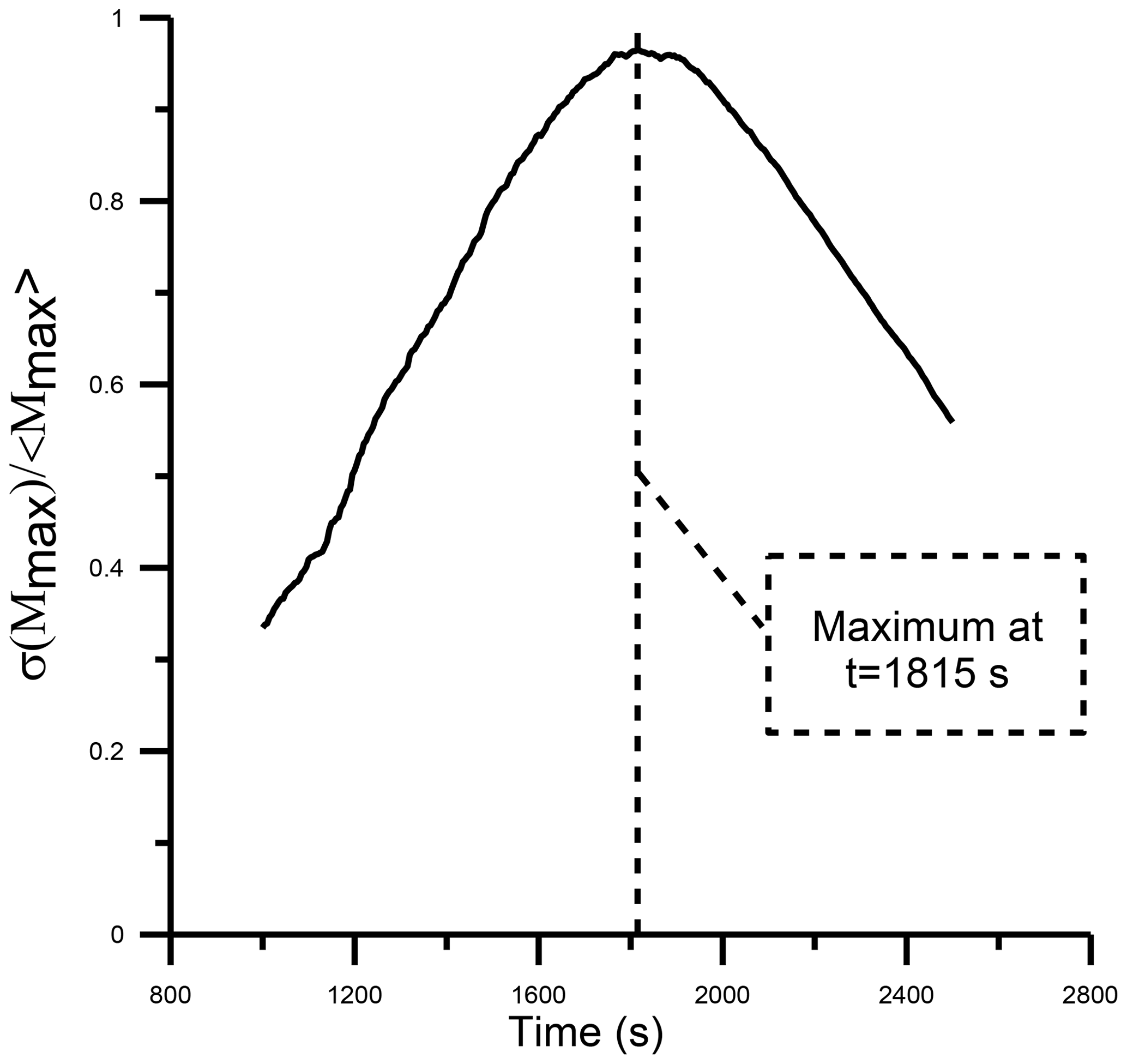
Figure 4Time evolution of the normalized standard deviation of the largest droplet mass versus time estimated from the Monte Carlo algorithm. The simulations were performed for the turbulent hydrodynamic kernel with a bi-disperse initial condition (200 droplets of 10 µm in radius and 50 droplets of 12.6 µm) in a volume of 1 cm3.

Figure 5Panels (a)–(d) (histograms) show the simulated Mmax distributions in a system with an initial bi-disperse distribution (200 droplets of 10 µm in radius and 50 droplets of 12.6 µm) at four different times. The solid line shows the fit using Eq. (6). The simulations were performed for the turbulent hydrodynamic kernel.
In this section, the methodology of analysis described before is applied to a dataset of cloud droplet size distribution (2–50 µm) collected with a Droplet Measurement Technologies fog monitor (FM-120) installed on a hilltop in Are, Sweden. The FM-120 is a single-particle optical spectrometer (Spiegel et al., 2012) that derives size from light scattered from individual droplets that pass through a focused laser beam. The equivalent optical size ranges from 2 to 50 µm. The fog monitor sample volume has a cross-sectional area of 0.25 mm2 and a flow speed of 14 m s−1. The raw data consist of each droplet's radius and inter-arrival time (elapsed time since previous particle). More than 7 million droplets were processed over a period of 4 h.
The block maxima (BM) approach in extreme value theory (EVT) was applied, which requires dividing the observation period into nonoverlapping periods of equal size and restricts attention to the maximum observation in each period (see Gumbel, 1958).
Following the BM approach, considering the sectional area and flow speed, the time series was divided into consecutive unit blocks of 1 cm3 in volume, corresponding to a cloud length of approximately 400 cm (∼0.3 s interval in the time series). The droplet distributions in each unit block are equivalent to the distributions obtained for each realization (for a fixed time) of the Monte Carlo algorithm described in the previous section, and each block can be interpreted as an independent realization of a stochastic process.
The maximum (radius of the largest droplet) is recorded from each consecutive unit block in order to generate the distribution for comparison with the theoretical combined distribution described in Eq. (6). The sample size corresponds to the number of consecutive blocks in which the time series was divided, which in this case is 49 647 blocks, equivalent to about 4 h of data. Figure 6 displays the number of droplets in each block, which fluctuate between 0 and 392, with an average of 146. Since each block is considered a realization of a random process, the largest droplet radius series must be fitted to the combined distribution in Eq. (6) for samples with certain conditions of homogeneity.

Figure 6Time series of the number of droplets per block, sampled at a hilltop in Are, Sweden.
The average sample size (number of unit blocks) for which the largest droplet maxima can be fitted to the combined distribution in Eq. (6) is then estimated. This expected value can be calculated from the following procedure.
The conditional probability P(Admixture|x), where x is the sample size, is calculated using Monte Carlo simulations. This calculation uses a given number of consecutive blocks with a mixture of distributions. The simulations are carried out by randomly choosing Ntotal samples from the measurements (that consist of consecutive blocks) of size x, fitting the data to the distribution in Eq. (6), and determining if they do or do not follow that distribution. The decision is based on application of the Kolmogorov–Smirnov (K-S) goodness of fit test for a confidence level α=0.05. The experimental statistics for the K-S test can be obtained by arranging the data in ascending order () and deriving the maximum difference between the rank statistics and the theoretically calculated cumulative density function F(xi):
If this value of Dn is smaller than a certain threshold value , we accept that the data obey the probability distribution under consideration, and the null hypothesis H0 cannot be rejected at a significance level α. The significance level α refers to the probability of the assumed distribution pattern being rejected. The limiting values of can be calculated from the K-S cumulative distribution (see Eqs. 5a and 5b). Tables with limiting values can be found in, e.g., Gnedenko (2017).
However, given that the parameters of the distribution F(x) were estimated from the observed data, theoretical limiting values provided by the K-S cannot be used. In this case, the limiting values are smaller than the case with known parameters and must be obtained via Monte Carlo simulations (see Appendix C for more details). Thus, the conditional probability can be calculated as follows:
where N0 is the number of cases for which the null hypothesis H0) at α=0.05 cannot be rejected. However, what is really needed is the conditional probability P(x|Admixture), which is the probability that a sample has size x, given that the data (viewed as a time series of maxima for each block) in that sample follow a mixture of distributions. This probability can be calculated using Bayes' theorem from the following expression:
By writing this theorem in the form (14), we are assuming that the marginal likelihood is considered a normalization factor. Therefore, P(x|Admixture) can be computed using expression (14) and then normalized under the requirement that it is a probability mass function (pmf). In Eq. (14), the prior probability π(x) is assumed to have a uniform distribution. Thus, the expected value 〈x〉 can be calculated from the following expression:
Turning to a concrete example, Ntotal=100 samples with sizes were randomly selected from the data, and the probability P(Admixture|x) calculated following Eq. (13). The probability mass function P(x|Admixture) (pmf) was obtained by applying the procedure previously described and the expected value was found to be 〈x〉=544 (about 163 s).
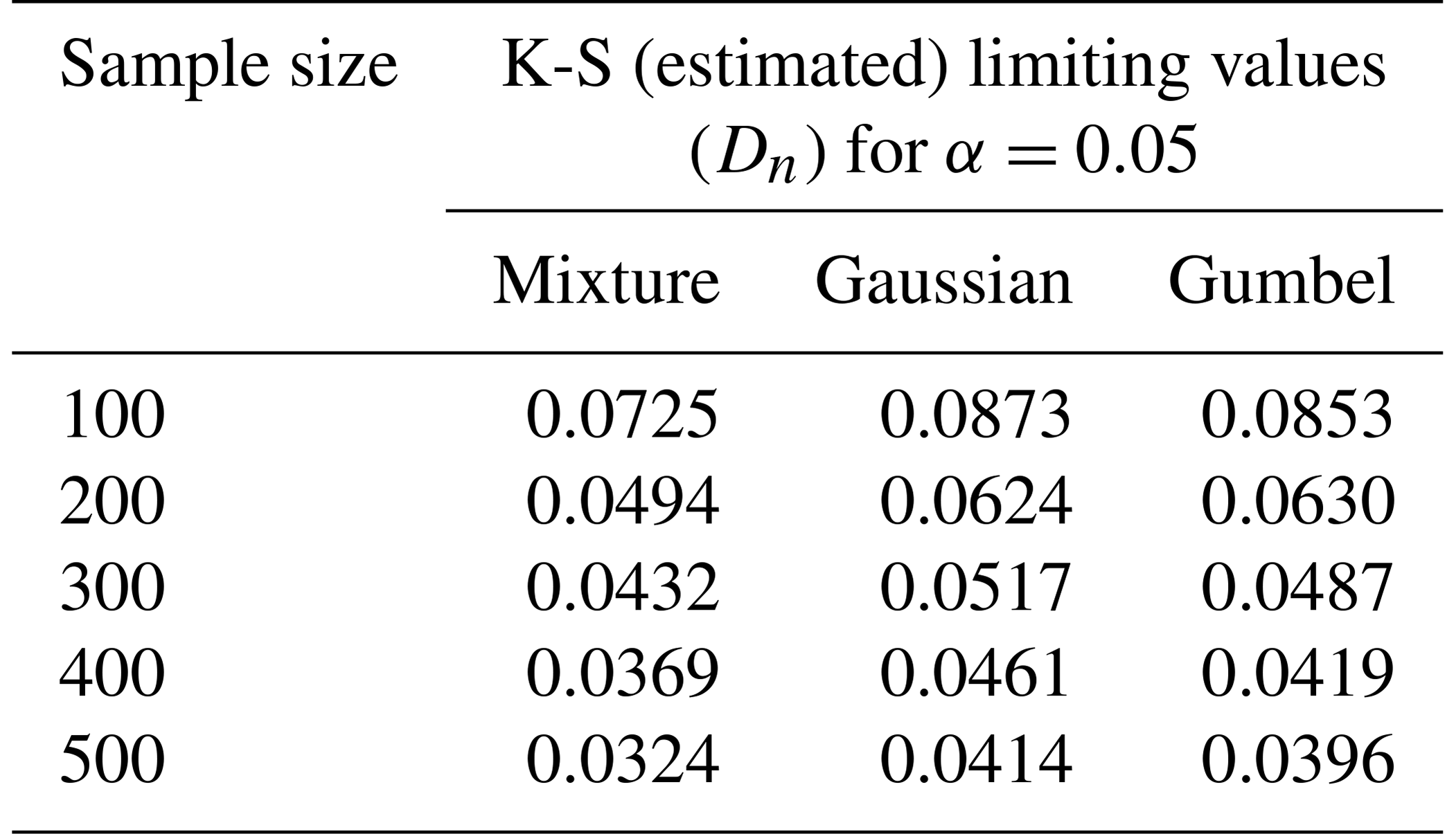
A thorough statistical analysis was conducted by fitting Mmax to the combined distribution in Eq. (6) for 100 samples with sizes at and below the average (100, 200, 300, …, 500) that were randomly selected from the entire dataset (49 647 blocks). For each random sample three null (H0) hypotheses were verified: (i) the sample comes from a mixture of distributions (Eq. 6), (ii) the sample comes from a Gumbel distribution or (iii) the sample comes from a Gaussian distribution. The three hypotheses were examined by the K-S method with limiting values calculated from Monte Carlo simulations (see Table C1).
The results for sample sizes 100, 200, 300, 400 and 500 are shown in Table 1. As an example, for case 1 (sample size 100) the null hypothesis H0 at α=0.05 was rejected for 13, 35 and 92 samples for the mixture, Gaussian and Gumbel distributions, respectively. For case 2 (sample size 200), the null hypothesis was rejected for 27, 58 and 96 samples. Using n=500 for the mixture of distributions (Eq. 6), the null hypothesis H0 was rejected for 50 samples. For the Gumbel distribution, the null hypothesis was rejected for all the samples (100) and the null hypothesis for the Gaussian distributions was rejected for 83 samples.
Table 1For each sample size, the number of samples with the null hypothesis H0 rejected at α=0.05 for all the distributions.
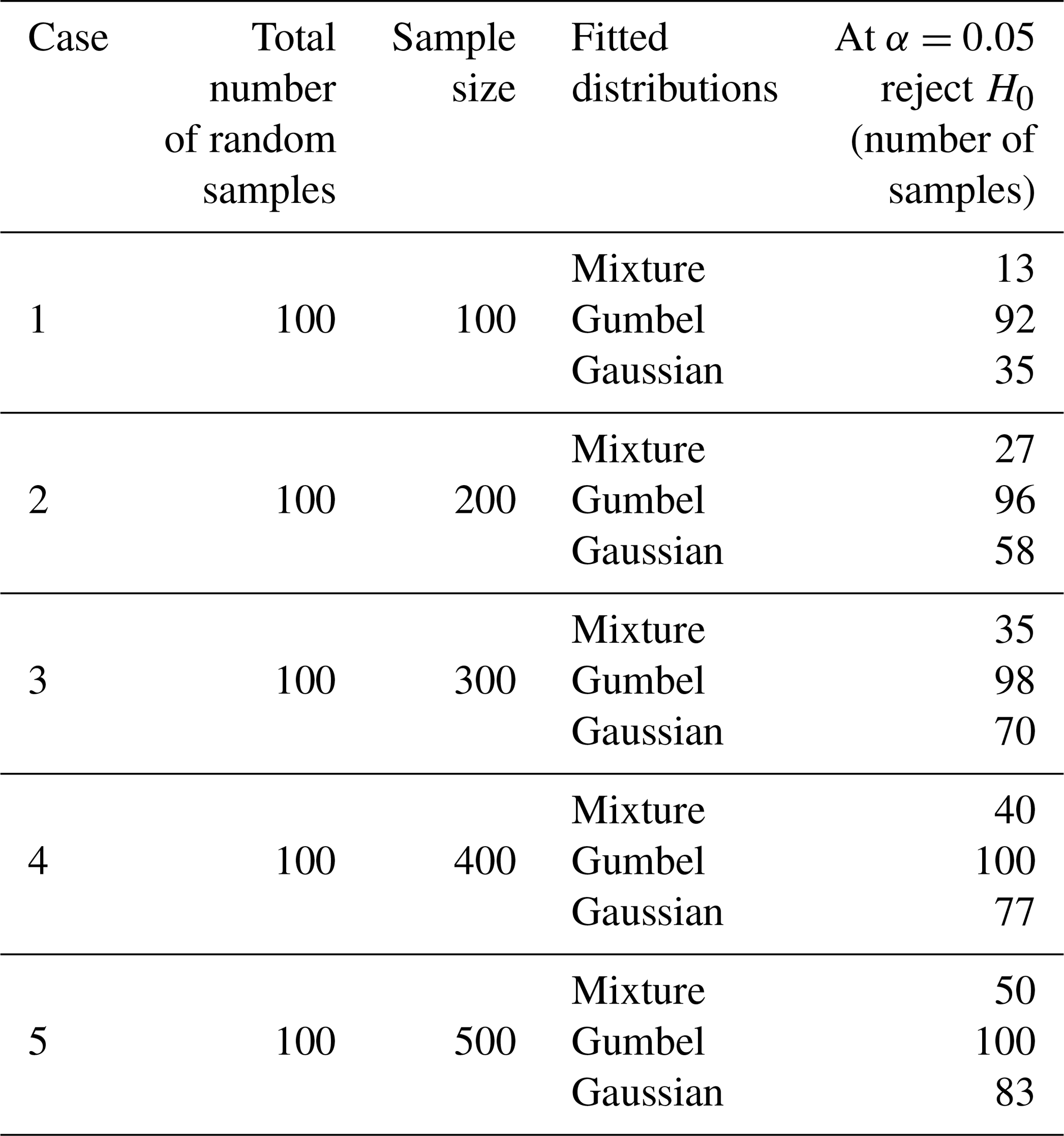
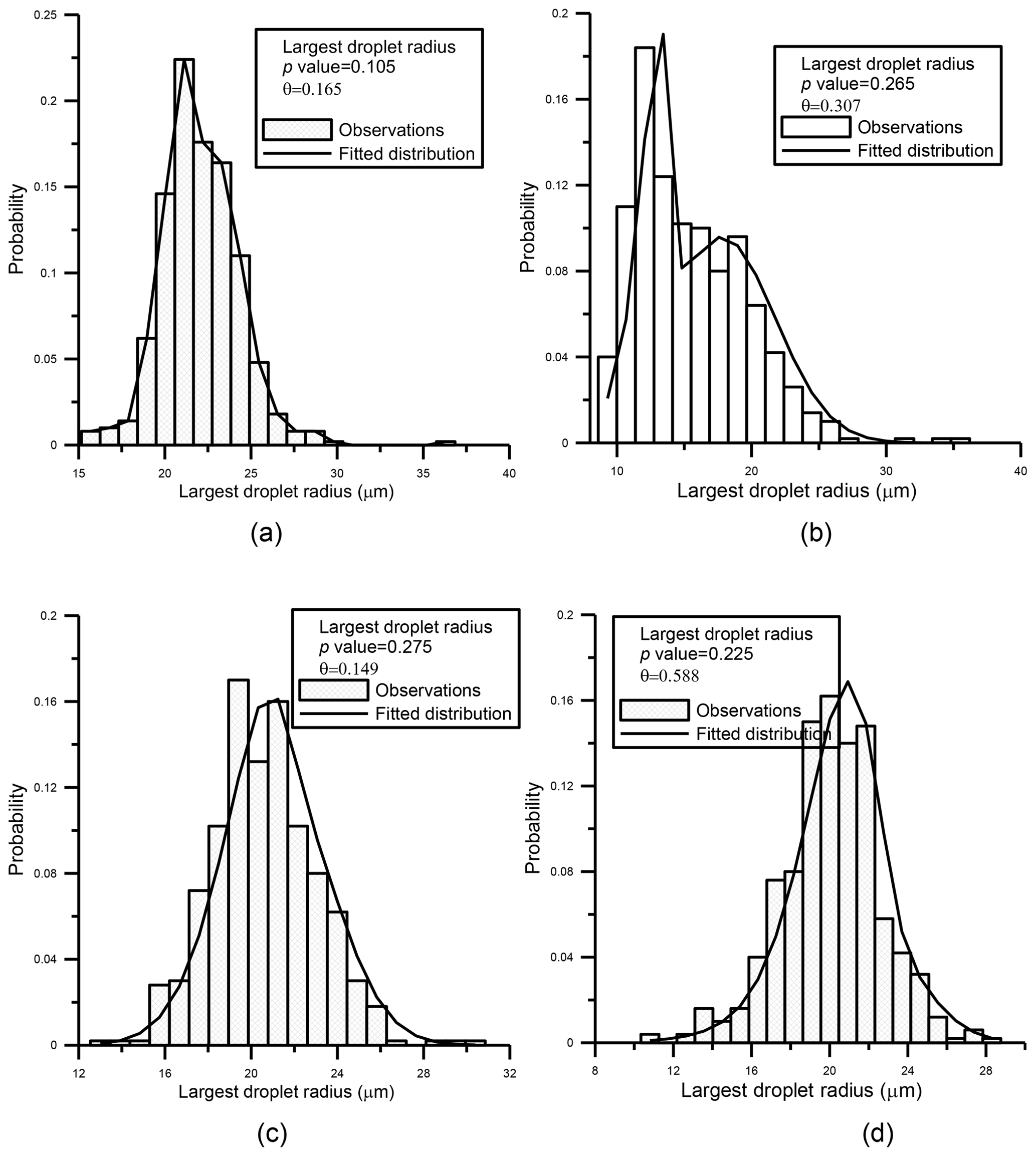
Figure 7For four random samples that are distributed following the admixture distribution (with sample size 500), observed (histogram) and fitted (solid line) using Eq. (6). Also shown for each distribution are the p value of the goodness of fit test and the parameter θ indicating the weight of the Gumbel component.
The results shown in Table 1 confirm that, for all sample sizes, the mixture of distributions provides a better fit than the Gumbel and Gaussian distributions, confirming the correctness of the choice of the mixture of distributions (Eq. 6) for modeling the largest droplet radius. As an example, Fig. 7a–d present, for a sample size of n=500, the largest droplet mass empirical distributions obtained for four different samples that are distributed following the mixture and the corresponding fit of Eq. (6).
An infinite system has two possible evolutionary phases: the ordered phase and the disordered or statistical phase. In the disordered phase there is a continuous droplet distribution and a near equality of the largest and second-largest mass. After the sol–gel transition, there is an ordered phase characterized by the existence of a giant macroscopic droplet (gel) coexisting with an ensemble of microscopic particles.
A finite system can be in the ordered, disordered and pseudo-critical phases, according to the scenario described in Botet (2011) and Gruyer et al. (2013). The ratio η, defined in Eq. (8), takes values between , −1, which correspond to pure Gaussian and Gumbel distributions, and when the system is in the pseudo-critical domain. In the disordered phase, fluctuations and correlations are negligible, there are only a few collision events, and Mmax is the largest part of randomly distributed droplets. In that case, the distribution of the mass of the largest droplets follow a Gumbel distribution. At later times in the evolution of the finite system, there are many collision events and Mmax is the result of the coalescence of other droplets. There is an additive process, the central limit theorem applies and the mass (or radius) of the largest droplets follows a Gaussian distribution.
In the pseudo-critical phase, the fluctuations and correlations are no longer negligible and the distribution is of neither of the asymptotic forms (Gumbel or Gaussian). In this case, the fit of the largest droplet mass (gel), is a mixture of a Gumbel (disordered state) and Gaussian (ordered state) distributions. As was demonstrated in the preceding section, this combined distribution (Eq. 6) is a good approximation to the largest droplet distribution (gel) in the pseudo-critical region. The fact that the mixture of distributions provides a better fit than the Gumbel and Gaussian distributions shows that the samples selected in our study are mainly in the pseudo-critical phase. To confirm this fact, the ratio η was calculated for 1000 samples of size n=500 selected randomly from the data. Figure 8 shows that for 90 % of the samples the ratio η lies in the interval [−0.9, 0.9], clearly indicating that samples are in the pseudo-critical region.
We could show that the gel radius (largest droplet) is described as a mixture of the two asymptotic distributions because the effect of the collision–coalescence process was in some way isolated for the orographic cloud data analyzed in this report. A similar analysis could be performed for the early stage of a convective cloud formation, before some other processes, e.g., entrainment, mixing, turbulence or ice formation, could obscure the finite system pseudo-critical scenario, and the gel formation that is basically a consequence of the collision–coalescence process could no longer be observed.
In this work, the early stage of formation of a warm cloud is viewed in the context of critical phenomena theory and can be thought of as being in ordered, disordered or pseudo-critical phases. The disordered phase corresponds to a cloud with a droplet spectrum formed mainly by the cloud condensation nuclei activation process, with an almost random distribution of particles, and the distribution of the mass of the largest droplets is Gumbel. In the pseudo-critical phase a giant droplet (gel) locally coexists with a continuous ensemble of small droplets. As the system considered is finite, there is no sudden change from disordered to ordered phase (sol–gel transition), but instead there is a pseudo-critical phase in which fluctuations are important and the gel distributes according to Eq. (6). The analysis presented here of the largest droplet distribution provides useful insight into the early stages of cloud development in warm clouds. In follow-up studies, the analysis of cloud data at different times or distances from the cloud base would be helpful in identifying the pseudo-critical phase and tracking the transition from the disordered to the ordered phase dynamically.
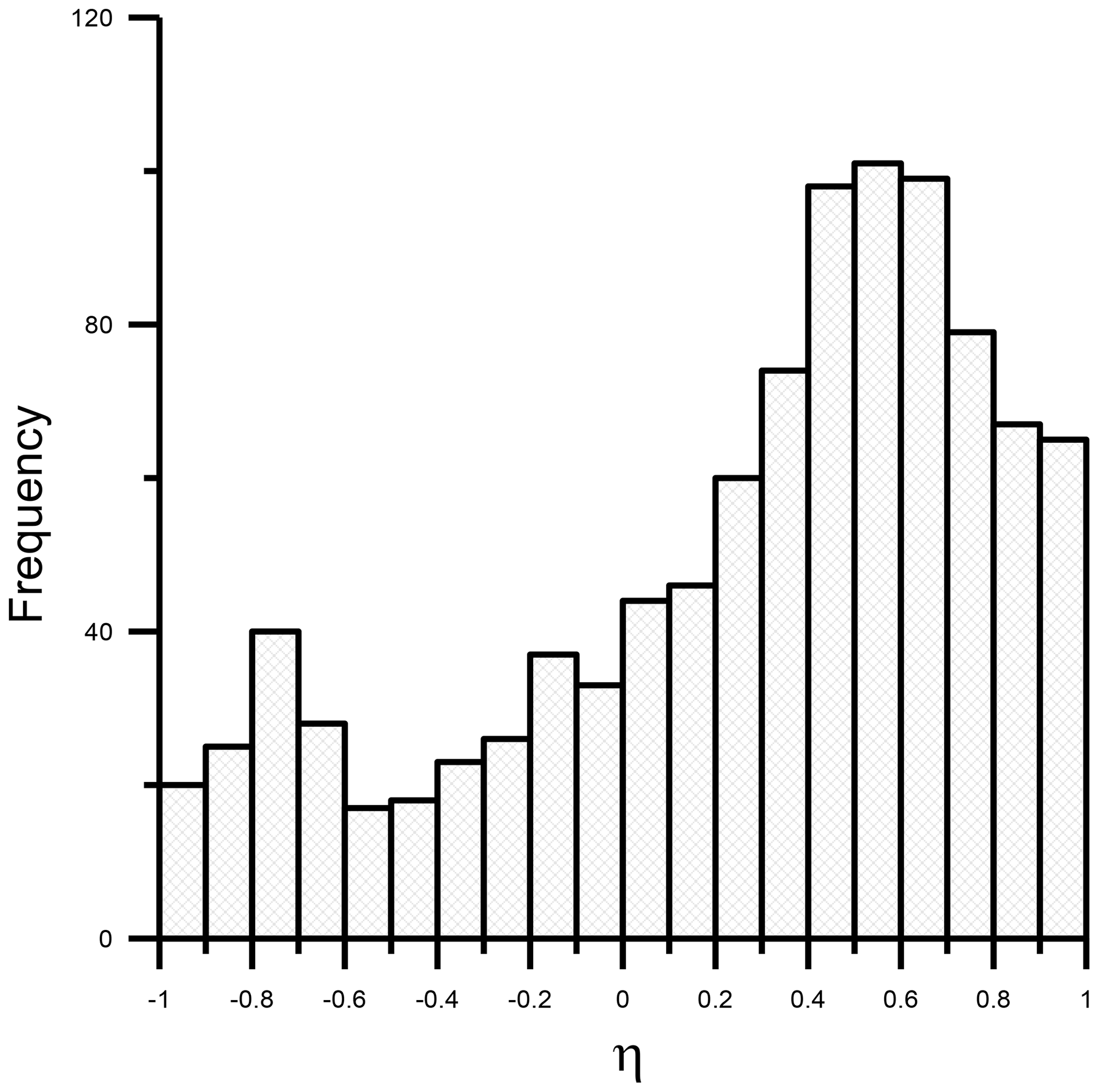
Figure 8Histogram of the ratio (wGaussian+wGumbel), which measures the distance to the critical point.
Access to the data used to produce the results discussed in this paper are available from the first author upon request by email.
The sol–gel transition time Tgel is defined as the time when the second moment becomes infinite, then and . The equation for M2(t) (moment of order 2 with respect to mass) can be found from the general equation for moment evolution that was obtained by Drake (1972) from the continuous form of the kinetic collection Eq. (1). It has the following form:
In Eq. (7), K(x,y) is the collection kernel, N(x,t) is the average droplet concentration and x is the droplet mass. If we consider the product kernel in Eq. (A1), then the equation for the second moment is
with the solution being .
After Tgel, a runaway droplet forms, and the kinetic collection equation is no longer valid, since the assumption of a continuous distribution breaks down. There is, in essence, a phase transition in the system from a continuous distribution to a continuous distribution plus a runaway droplet.
In this study, the species accounting formulation (Laurenzi et al., 2002) of the stochastic simulation algorithm (SSA) of Gillespie (1975) was used for the stochastic simulation. The steps below summarize the algorithm:
-
Initialization. Initialize the number of droplets in each species (the species are defined as droplets of different sizes). There is a unique index μ for each pair of droplets i,j that may collide. For a system with N species, . The set {μ} defines the total collision space and is equal to the total number of possible interactions.
-
Monte Carlo step. Determine the next collision to occur and the time to the next collision. The next collision μ is calculated according to the distribution , from the inequality:
where r2 is a uniformly distributed random number in the interval (0,1). aμ is calculated from the following probabilities:
-
two unlike particles i and j with populations (number of particles) ni and nj will collide within the imminent time interval},
-
two particles of the same species i with population (number of particles) ni collide within the imminent time interval},
-
.
As the time to the next collision is exponentially distributed with mean 1∕α (Gillespie, 1975) and is a uniformly distributed random number in the interval [0,1], the time τ to the next collision can be calculated from the following expression:
-
-
Increase the time by the randomly generated time in Step 2. Change the numbers of species to reflect the execution of a collision.
-
If stopping criteria are not met, go to step 2.
When parameters of a distribution are estimated from the data, the limiting values provided for the Kolmogorov–Smirnov criterion cannot be used. In this case, approximate limiting values and p values can be obtained via Monte Carlo simulations. First, the parameter vector is estimated for a given sample of size n, and the test statistics (Eq. 12) are calculated assuming that the sample is distributed according to , returning a value of Dn. Next, a sample of size variates is generated, and the parameter vector is estimated. The test statistics are calculated again assuming that the sample is distributed according to . Such a calculation was made for different sample sizes () 1000 times, and the distribution pattern of Dn was derived (see Table C1). Thus, 5 % (for α=0.05) from the greater side was taken as the estimated limiting values. The estimate of p value is calculated as the relative number of occasions in which the test statistics are at least as large as Dn. The numerically calculated K-S limiting values for the three distributions under analysis (mixture, Gumbel and Gaussian) for α=0.05 are shown in Table C1. As can be checked, the values are smaller than the case with known parameters, which can be estimated (for α=0.05) as .
Table C1Estimated limiting values (for α=0.05) for the Kolmogorov–Smirnov goodness of fit test for the three distributions.
LA performed the model runs of the Monte Carlo algorithm, performed the statistical analysis of synthetic and observational data, and wrote the paper. GBR and DB provided the observational data and edited and improved the paper. All authors contributed to developing the basic ideas and discussing the results.
The authors declare that they have no conflict of interest.
This study was funded by a grant from the Consejo Nacional de Ciencia y Tecnología of Mexico (SEP-Conacyt) CB-284482. We also thank the two anonymous reviewers for their helpful comments on our paper.
This research has been supported by the Consejo Nacional de Ciencia y Tecnología (grant no. CB-284482.).
This paper was edited by Sachin S. Gunthe and reviewed by two anonymous referees.
Aldous, D. J.: Deterministic and stochastic models for coalescence (aggregation, coagulation): A review of the mean-field theory for probabilistic, Bernoulli, 5, 3–48, 1999.
Alfonso, L.: An algorithm for the numerical solution of the multivariate master equation for stochastic coalescence, Atmos. Chem. Phys., 15, 12315–12326, https://doi.org/10.5194/acp-15-12315-2015, 2015.
Alfonso, L. and Raga, G. B.: The impact of fluctuations and correlations in droplet growth by collision–coalescence revisited – Part 1: Numerical calculation of post-gel droplet size distribution, Atmos. Chem. Phys., 17, 6895–6905, https://doi.org/10.5194/acp-17-6895-2017, 2017.
Alfonso, L., Raga, G. B., and Baumgardner, D.: The validity of the kinetic collection equation revisited, Atmos. Chem. Phys., 8, 969–982, https://doi.org/10.5194/acp-8-969-2008, 2008.
Alfonso, L., Raga, G. B., and Baumgardner, D.: The validity of the kinetic collection equation revisited – Part 2: Simulations for the hydrodynamic kernel, Atmos. Chem. Phys., 10, 7189–7195, https://doi.org/10.5194/acp-10-7189-2010, 2010.
Alfonso, L., Raga, G. B., and Baumgardner, D.: The validity of the kinetic collection equation revisited – Part 3: Sol–gel transition under turbulent conditions, Atmos. Chem. Phys., 13, 521–529, https://doi.org/10.5194/acp-13-521-2013, 2013.
Baker, M., Corbin, R. G., and Latham, J.: The influence of entrainment on the evolution of cloud drop spectra: I. A model of inhomogeneous mixing, Q. J. Roy. Meteor. Soc., 106, 581–598, 1980.
Bayewitz, M. H., Yerushalmi, J., Katz, S., and Shinnar, R.: The extent of correlations in a stochastic coalescence process, J. Atmos. Sci., 31, 1604–1614, 1974.
Bazant, M. Z.: Largest cluster in subcritical percolation, Phys. Rev. E, 62, 1660, https://doi.org/10.1103/PhysRevE.62.1660, 2000.
Beard, K. V. and Ochs, H. T.: Warm-rain initiation – An overview of microphysical mechanisms, J. Appl. Meteorol., 32, 608–625, 1993.
Bhattacharjee, S. M.: Critical Phenomena: An Introduction from a modern perspective, in: Field Theories in Condensed Matter Physics, 69–117, Hindustan Book Agency, Gurgaon, 2001.
Botet, R.: Where are correlations hidden in the distribution of the largest fragment?, PoS, 007, WPCF2011, 2011.
Botet, R. and Płoszajczak, M.: Exact order-parameter distribution for critical mean-field percolation and critical aggregation, Phys. Rev. Lett., 95, 185702, https://doi.org/10.1103/PhysRevLett.95.185702, 2005.
Botet, R., Płoszajczak, M., Chbihi, A., Borderie, B., Durand, D., and Frankland, J.: Universal fluctuations in heavy-ion collisions in the Fermi energy domain, Phys. Rev. Lett., 86, 3514, https://doi.org/10.1103/PhysRevLett.86.3514, 2001.
Chen, S., Yau, M. K., and Bartello, P.: Turbulence effects of collision efficiency and broadening of droplet size distribution in cumulus clouds, J. Atmos. Sci., 75, 203–217, https://doi.org/10.1175/JAS-D-17-0123.1, 2018.
Clusel, M. and Bertin, E.: Global fluctuations in physical systems: a subtle interplay between sum and extreme value statistics, Int. J. Mod. Phys. B, 22, 3311–3368, 2008.
Cooper, W. A.: Effects of variable droplet growth histories on droplet size distributions. Part I. Theory, J. Atmos. Sci., 46, 1301–1311, 1989.
Drake, R. L.: The scalar transport equation of coalescence theory: Moments and kernels, J. Atmos. Sci., 29, 537–547, 1972.
Drake, R. L. and Wright, T. J.: The scalar transport equation of coalescence theory: New families of exact solutions, J. Atmos. Sci., 29, 548–556, 1972.
Dziekan, P. and Pawlowska, H.: Stochastic coalescence in Lagrangian cloud microphysics, Atmos. Chem. Phys., 17, 13509–13520, https://doi.org/10.5194/acp-17-13509-2017, 2017.
Falkovich, G. and Pumir, A.: Sling effect in collisions of water droplets in turbulent clouds, J. Atmos. Sci., 64, 4497–4505, 2007.
Feingold, G. and Chuang, P. Y.: Analysis of the influence of film-forming compounds on droplet growth: Implications for cloud microphysical processes and climate, J. Atmos. Sci., 59, 2006–2018, 2002.
Feingold, G., Cotton, W. R., Kreidenweis, S. M., and Davis, J. T.: The impact of giant cloud condensation nuclei on drizzle formation in stratocumulus: Implications for cloud radiative properties, J. Atmos. Sci., 56, 4100–4117, 1999.
Gillespie, D. T.: An Exact Method for Numerically Simulating the Stochastic Coalescence Process in a Cloud, J. Atmos. Sci., 32, 1977–1989, 1975.
Gnedenko, B. V.: Theory of probability, Chelsea Publishing Co., N.Y., 4th Edn., 2017.
Göke, S., Ochs, H. T., and Rauber, R. M.: Radar analysis of precipitation initiation in maritime versus continental clouds near the Florida coast: Inferences concerning the role of CCN and giant nuclei, J. Atmos. Sci., 64, 3695–3707, https://doi.org/10.1175/JAS3961.1, 2007.
Golovin, A. M.: The Solution of the Coagulation Equation for Raindrops. Taking Condensation into Account, Soviet Physics Doklady, Vol. 8, 191–193, 1963.
Grabowski, W. W. and Wang, L.-P.: Growth of cloud droplets in a turbulent environment, Annu. Rev. Fluid Mech., 45, 293–324, 2013.
Gruyer, D., Frankland, J. D., Botet, R., Płoszajczak, M., Bonnet, E., Chbihi, A., … and Guinet, D.: Nuclear multifragmentation time scale and fluctuations of the largest fragment size, Phys. Rev. Lett., 110, 172701, https://doi.org/10.1103/PhysRevLett.110.172701, 2013.
Gumbel, E. J.: Statistics of extremes, Columbia University Press, New York, 1958.
Hall, W. D.: A detailed microphysical model within a two-dimensional dynamic framework: Model description and preliminary results, J. Atmos. Sci., 37, 2486–2507, 1980.
Inaba, S., Tanaka, H., Ohtsuki, K., and Nakazawa, K.: High accuracy statistical simulation of planetary accretion: I. Test of the accuracy by comparison with the solution to the stochastic coagulation equation, Earth Planets Space, 51, 205–217, 1999.
Johnson, D. B.: The role of giant and ultragiant aerosol particles in warm rain initiation, J. Atmos. Sci., 39, 448–460, 1982.
Kolb, M. and Axelos, A. V.: Gelation Transition versus Percolation Theory, in: Correlations and Connectivity, Springer, Dordrecht, 255–261, 1990.
Kostinski, A. B. and Shaw, R. A.: Fluctuations and luck in droplet growth by coalescence, B. Am. Meteorol. Soc., 86, 235–244, 2005.
Laurenzi, I. J., Bartels, J. D., and Diamond, S. L.: A general algorithm for exact simulation of multicomponent aggregation processes, J. Comput. Phys., 177, 418–449, 2002.
Li, X.-Y., Brandenburg, A., Haugen, N. E. L., and Svensson, G.: Eulerian and Lagrangian approaches to multidimensional condensation and collection, J. Adv. Model. Earth Sy., 9, 1116–1137, https://doi.org/10.1002/2017MS000930, 2017.
Li, X.-Y., Brandenburg, A., Svensson, G., Haugen, N. E. L., Mehlig, B., and Rogachevskii, I.: Effect of Turbulence on Collisional Growth of Cloud Droplets, J. Atmos. Sci., 75, 3469–3487, https://doi.org/10.1175/JAS-D-18-0081.1, 2018.
Long, A.: Solutions to the droplet collection equation for polynomial kernels, J. Atmos. Sci., 31, 1040–1052, 1974.
Lushnikov, A. A.: Coagulation in finite systems, J. Colloid Interf. Sci., 65, 276–285, 1978.
Lushnikov, A. A.: From sol to gel exactly, Phys. Rev. Lett., 93, 198302, https://doi.org/10.1103/PhysRevLett.93.198302, 2004.
Lushnikov, A. A., Negin, A. E., and Pakhomov, A. V.: Experimental observation of the aerosol-aerogel transition, Chem. Phys. Lett., 175, 138–142, 1990.
Marcus, A. H.: Stochastic coalescence, Technometrics, 10, 133–143, 1968.
Matsoukas, T.: Statistical Thermodynamics of Irreversible Aggregation: The Sol-Gel Transition, Sci. Rep.-UK, 5, 8855, https://doi.org/10.1038/srep08855, 2015.
Onishi, R. and Seifert, A.: Reynolds-number dependence of turbulence enhancement on collision growth, Atmos. Chem. Phys., 16, 12441–12455, https://doi.org/10.5194/acp-16-12441-2016, 2016.
Pinsky, M. B. and Khain, A. P.: Collisions of small drops in a turbulent flow. Part II: Effects of flow accelerations, J. Atmos. Sci., 61, 1926–1939, 2004.
Pinsky, M. B., Khain, A. P., and Shapiro, M.: Collisions of cloud droplets in a turbulent flow. Part IV: Droplet hydrodynamic interaction, J. Atmos. Sci., 64, 2462–2482, 2007.
Pinsky, M., Khain, A., and Krugliak, H.: Collisions of cloud droplets in a turbulent flow. Part V: Application of detailed tables of turbulent collision rate enhancement to simulation of droplet spectra evolution, J. Atmos. Sci., 65, 357–374, 2008.
Pruppacher, H. R. and Klett, J. D.: Microphysics of clouds and precipitation, Kluwer Academic Publishers, Dordrecht, the Netherlands, 1997.
Roach, W. T.: On the effect of radiative exchange on the growth by condensation of a cloud or fog droplet, Q. J. Roy. Meteor. Soc., 102, 361–372, 1976.
Scott, W. T.: Analytic studies of cloud droplet coalescence, J. Atmos. Sci., 25, 54–65, 1968.
Shaw, R. A., Reade, W. C., Collins, L. R., and Verlinde, J.: Preferential concentration of cloud droplets by turbulence: Effects on the early evolution of cumulus cloud droplet spectra, J. Atmos. Sci., 55, 1965–1976, 1998.
Shima, S.-I., Kusano, K., Kawano, A., Sugiyama, T., and Kawahara, S.: The super-droplet method for the numerical simulation of clouds and precipitation: A particle-based and probabilistic microphysics model coupled with a non-hydrostatic model, Q. J. Roy. Meteor. Soc., 135, 1307–1320, 2009.
Sidin, R. S., Hagmeijer, R., and Sachs, U.: Evaluation of master equations for the droplet size distribution in condensing flow, Phys. Fluids, 21, 073303, https://doi.org/10.1063/1.3180863, 2009.
Spiegel, J. K., Zieger, P., Bukowiecki, N., Hammer, E., Weingartner, E., and Eugster, W.: Evaluating the capabilities and uncertainties of droplet measurements for the fog droplet spectrometer (FM-100), Atmos. Meas. Tech., 5, 2237–2260, https://doi.org/10.5194/amt-5-2237-2012, 2012.
Tanaka, H. and Nakazawa, K.: Stochastic coagulation equation and the validity of the statistical coagulation equation, J. Geomagn. Geoelectr., 45, 361–381, 1993.
Tanaka, H. and Nakazawa, K.: Validity of the statistical coagulation equation and runaway growth of protoplanets, Icarus, 107, 404–412, 1994.
Telford, J.: A new aspect of coalescence theory, J. Meteorol., 12, 436–444, 1955.
Touchette, H.: The large deviation approach to statistical mechanics, Phys. Rep., 478, 1–69, 2009.
Van den Heever, S. C. and Cotton, W. R.: Urban aerosol impacts on downwind convective storms, J. Appl. Meteorol. Clim., 46, 828–850, 2007.
Wang, L.-P., Ayala, O., Rosa, B., and Grabowski, W. W.: Turbulent collision efficiency of heavy particles relevant to cloud droplets, New J. Phys., 10, 075013, https://doi.org/10.1088/1367-2630/10/7/075013, 2008.
Warner, J.: The microstructure of cumulus cloud. Part I. General features of the droplet spectrum, J. Atmos. Sci., 26, 1049–1059, 1969.
Wetherill, G. W.: Comparison of analytical and physical modeling of planetesimal Accumulation, Icarus, 88, 336–354, 1990.
Wilkinson, M.: Large deviation analysis of rapid onset of rain showers, Phys. Rev. Lett., 116, 018501, https://doi.org/10.1103/PhysRevLett.116.018501, 2016.
Yin, Y., Levin, Z., Reisin, T. G., and Tzivion, S.: The effect of giant cloud condensation nuclei on the development of precipitation in convective clouds – A numerical study, Atmos. Res., 53, 91–116, 2000.
Zhang, H., Wang, X., You, M., and Liu, C.: Water-yield relations and water-use efficiency of winter wheat in the North China Plain, Irrigation Sci., 19, 37–45, 1999.
- Abstract
- Introduction
- An overview of previous theoretical and experimental results
- Analysis of the largest droplet distribution obtained from synthetic data
- Analysis of the largest droplet (gel) radius distribution from observations
- Discussion and conclusions
- Data availability
- Appendix A
- Appendix B: The Monte Carlo algorithm
- Appendix C: Procedure for estimating the limiting values for the Kolmogorov–Smirnov goodness of fit test for distributions with unknown parameters
- Author contributions
- Competing interests
- Acknowledgements
- Financial support
- Review statement
- References
lucky droplet) is a mixture of Gaussian and Gumbel distributions. The results obtained may help advance the understanding of precipitation formation and are a novel application of the theory of critical phenomena in cloud physics.
- Abstract
- Introduction
- An overview of previous theoretical and experimental results
- Analysis of the largest droplet distribution obtained from synthetic data
- Analysis of the largest droplet (gel) radius distribution from observations
- Discussion and conclusions
- Data availability
- Appendix A
- Appendix B: The Monte Carlo algorithm
- Appendix C: Procedure for estimating the limiting values for the Kolmogorov–Smirnov goodness of fit test for distributions with unknown parameters
- Author contributions
- Competing interests
- Acknowledgements
- Financial support
- Review statement
- References