2.1 Transport models

LMDz is the atmospheric component of the Earth system model of the Institut Pierre-Simon-Laplace (Dufresne et al., 2013) which has been contributing to the recent versions of the Climate Model Intercomparison Project (CMIP) established by the World Climate Research Programme (https://www.wcrp-climate.org/wgcm-cmip, last access: 21 November 2019). Here, we use its offline version (Hourdin et al., 2006) to simulate the transport of CO₂. The offline LMDz model reads a frozen archive of 3-hourly mean meteorological data pre-computed by the full LMDz so that it only needs to simulate large-scale advection and sub-grid transport processes (i.e. deep convection and boundary layer turbulence). LMDz is nudged towards 6-hourly analysed meteorological variables, here either ERA-Interim (Dee et al., 2011) or ERA5 (https://www.ecmwf.int/en/forecasts/datasets/archive-datasets/reanalysis-datasets/era5, last access: 31 January 2019) with a relaxation time of 3 h. Online and offline models are consistently run at the same spatial resolution in order to avoid any challenging interpolation of the air mass fluxes for the sub-grid processes (see e.g. Yu et al., 2018): here 39 eta-pressure layers between the surface and around 80 km above sea level (km a.s.l.), and 96 grid points × 96 grid points, i.e. a horizontal resolution of 1.89 in latitude × 3.75^∘ in longitude. This configuration discretises the 2–7 km a.s.l. region of the atmosphere, which will be a major focus in the following, into 6 to 10 layers, depending on local orography.

We use two physical formulations of LMDz, called 5A (in code identification number 1649) and 6A (in code identification number 3353), as described by Remaud et al. (2018, and references therein). The gap between the two versions represents about 6 years of development from the LMDz team and includes e.g. a complete revision of radiation, the introduction of the thermodynamical effect of ice and changes in the sub-grid-scale parameterisations (convection, boundary layer dynamics) and in the land surface processes. For version 5A, horizontal winds are nudged towards ERA-Interim, but we use the new ERA5 for LMDz6A. Therefore, the differences between the two versions cannot be exclusively attributed to sub-grid-scale processes, as boundary variables (nudging files and land processes) differ as well.

2.2 Inversion system

LMDz is embedded within the CAMS CO₂ inversion system. This system minimises a Bayesian cost function to optimise the grid cell 8-day surface fluxes (with a distinction between local night-time fluxes and daytime fluxes, but without fossil fuel emissions, which are prescribed) and the initial state of CO₂. To do so, it assimilates a series of CO₂ observations over a given time window within the LMDz model. The minimisation approach is called “variational” because it explicitly computes the gradient of the cost function using the adjoint code of LMDz. Prior information about the surface fluxes is provided to the Bayesian system by a combination of climatologies and other types of measurement-driven flux estimates (e.g. Emission Database for Global Atmospheric Research version 4.3.2, Crippa et al., 2016, scaled globally and annually from Le Quéré et al., 2018, for the fossil fuel emissions or Landschützer et al., 2017, for the ocean fluxes). Details can be found in Chevallier (2018a). Of special interest here is the fact that, when integrated over a calendar year, prior natural fluxes are zero over all land grid points: this implies that the interannual variability of the inferred annual mean of terrestrial vegetation fluxes is generated by the assimilated observations only. Over a full year, the total 1σ uncertainty (resulting from assigned error variances that vary in space and time, and from assigned temporal and spatial error correlations) for these prior land fluxes amounts to about 3.0 GtC a⁻¹. The error statistics for the open ocean correspond to a global air–sea flux uncertainty of about 0.5 GtC a⁻¹.

The assimilation window is either 19 years for the surface measurements (from January 2000 to October 2018), 8 years for the GOSAT retrievals (from January 2009 to December 2016) or 4 years for the OCO-2 retrievals (from September 2014 to July 2018).

2.3 Assimilated observations

All assimilated observations are the dry air mole fraction of CO₂.

Assimilated surface air sample measurements have been selected from four large ongoing databases of atmospheric CO₂ measurements: (i) NOAA's ObsPack (Cooperative Global Atmospheric Data Integration Project, 2018, and CarbonTracker Team, 2018), (ii) the World Data Centre for Greenhouse Gases archive (WDCGG, https://gaw.kishou.go.jp/, last access: 21 November 2019), (iii) the Réseau Atmosphérique de Mesure des Composés à Effet de Serre database (RAMCES, http://www.lsce.ipsl.fr/, last access: 21 November 2019) and (iv) the Integrated Carbon Observation System Atmospheric Thematic Centre (ICOS-ATC, https://icos-atc.lsce.ipsl.fr/, last access: 21 November 2019). The list of selected sites and maps of their location are given by Chevallier (2018a). Each dataset provides at least 5 years of measurements. The error variances assigned to these measurements in the inversion system correspond to transport modelling uncertainty (analytical measurement uncertainty of in situ CO₂ data is a negligible component) and are computed as the variance of the high-frequency variability of the de-seasonalised and de-trended CO₂ time series of the daily mean measurements at each site. These variances are then inflated in order to give the same weight to each measurement day at a given location.

GOSAT was launched in January 2009, as a joint project of the Japan Aerospace Exploration Agency (JAXA), the National Institute of Environmental Studies (NIES) and Japan's Ministry of the Environment (MOE) (Kuze et al., 2009). OCO-2 is a NASA satellite that was launched in July 2014 (Eldering et al., 2017). Both satellites still collect scientific data today. They orbit around the Earth from pole to pole with a local crossing time at the Equator in the early local afternoon. Each carries a spectrometer that measures the sunlight reflected by the Earth and its atmosphere in the near-infrared/shortwave infrared spectral regions, with high spectral resolution ($>\sim$ 20 000) such that individual gas absorption lines are resolved. OCO-2 provides spatially dense data with a narrow swath and with footprints of a few square kilometres, whereas GOSAT provides coarser-resolution data (100 km² at nadir) with low spatial density. Various algorithms have been developed to retrieve the column-average dry air mole fraction of CO₂ in the atmosphere (XCO₂) from the measured radiance spectrums. For GOSAT, we use bias-corrected XCO₂ retrievals from the OCO Full Physics (OCFP) v7.1 product made by the University of Leicester and available from the Copernicus Climate Change Service for the period from April 2009 to December 2016 (https://climate.copernicus.eu/, last access: 21 November 2019). For OCO-2, we use NASA's Atmospheric CO₂ Observations from Space (ACOS) bias-corrected retrievals, version 9 (Kiel et al., 2019; O'Dell et al., 2018) from September 2014 to July 2018. In both cases, a previous release of the CAMS surface-based inversion contributed to the retrieval official bias-correction to some extent. We neglect this dependency in the following because other reference data are used that reduce the weight of the CAMS inversion (e.g. TCCON), and because the bias-correction schemes rely on two to five time- and space- invariant parameters only, with internal retrieval variables (e.g. the retrieved vertical CO₂ gradient between the surface and the free troposphere) as predictors. We do not tune the official retrieval bias corrections. To reduce data volume without loss of information at the scale of a global model, glint and nadir OCO-2 retrievals have been averaged in 10 s bins for the Model Intercomparison Project (MIP) of OCO-2, as described in Crowell et al. (2019), and we use them in this form. The retrieval averaging kernels, prior profiles and Bayesian uncertainty are accounted for in the assimilation of both types of satellite retrievals (the interpolation procedure between the model vertical grid and the retrieval grid is described in Sect. 2.2 of Chevallier, 2015). For OCO-2 retrievals, we also use the transport uncertainty term that is provided by the OCO-2 MIP, based on the variability across several models at the OCO-2 sounding locations (Crowell et al., 2019).

Maps of the coverage of GOSAT and OCO-2 retrievals are shown in Bösch and Anand (2017) and O'Dell et al. (2018), respectively. We only consider “good” retrievals as identified by the xco2_quality_flag variable of each product. Both land and ocean data are used for GOSAT. GOSAT data over ocean have matured in the ∼10 years since they were first produced, and have reached a point where they appear to have smaller biases than over land (Zhou et al., 2016). Their direct inclusion in inversions also appears to be beneficial (Deng et al., 2016). However, although the ocean biases in OCO-2 have been substantially reduced since the initial version 7 (O'Dell et al., 2018), initial inversion tests using OCO-2 ocean observations still produced highly unrealistic results (annual global ocean sinks of about 5 GtC a⁻¹ compared with the much smaller state-of-the-art estimates in Le Quéré et al., 2018) and are therefore left out of this work (as are retrievals over inland water or over mixed land–water surfaces). As for GOSAT, this situation may change in time and OCO-2 ocean data could be beneficial in future inversion set-ups. Despite the exclusion of ocean retrievals and the 10 s averaging, there are still 65 % more OCO-2 retrievals than GOSAT retrievals assimilated on average per month.

2.4 Verification observations

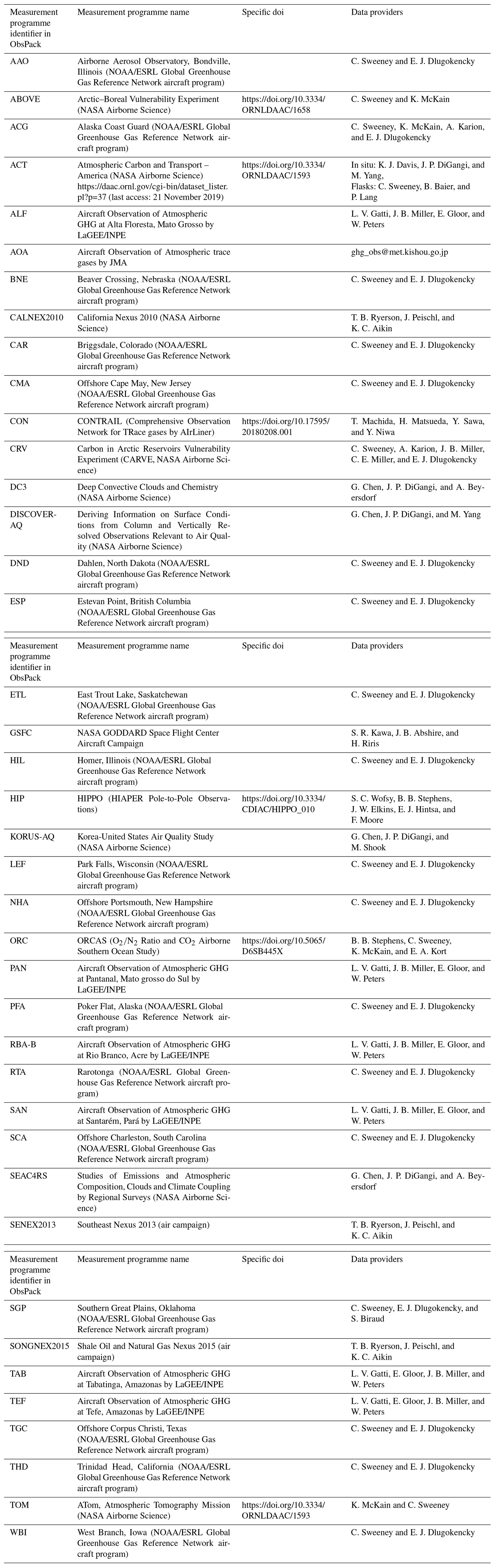
We use some specific measurements of the dry air mole fraction of CO₂ as verification data. They are aircraft measurements in the free troposphere made between July 2009 and December 2017 and archived in different ObsPacks (Cooperative Global Atmospheric Data Integration Project, 2018, and NOAA Carbon Cycle Group ObsPack Team, 2018). Table 1 lists the various aircraft measurement sites, campaigns or programmes. For simplicity, all sites, campaigns or programmes will be referred to as “programmes” in the following. All measurements have been calibrated to the WMO CO₂ X2007 scale or to the NIES 09 CO₂ scale to better than 0.1 ppm (e.g. Machida et al., 2008; Sweeney et al., 2015). We note that no aircraft data are assimilated here (Sect. 2.3).

Table 1Aircraft measurement programmes used here. Note that the ALF, PAN, RBA-B, SAN and TEF programmes are gathered under the identifier “INPE” (for Instituto Nacional de Pesquisas Espaciais) in Fig. 8.

Download XLSX

We define the free troposphere as the altitudes between 2 and 7 km a.s.l. We avoid data below 2 km because (i) local anthropogenic emissions affect many aircraft measurements there, and (ii) some of the aircraft flew in the vicinity of measurement sites that have been used in the surface-based inversions. We avoid data above 7 km because the measurement variations (and the flux regional signal) are much reduced there. A few outliers for which the difference between model and observation is larger than 40 ppm are rejected: they likely represent very local pollution plumes.

We define two periods for the following statistical computations. They are based on the availability of the satellite retrievals and of the aircraft data in the databases used here: a “GOSAT period” from July 2009 to September 2016 and an “OCO-2 period” from December 2014 to December 2017. Note that they overlap and that there is a minimum of 3 months between the temporal bounds of the verification data and the temporal bounds of the assimilated data in order to account for inversion spin-up and spin-down. Figure 1 shows the geographical location of the verification data for the two periods.

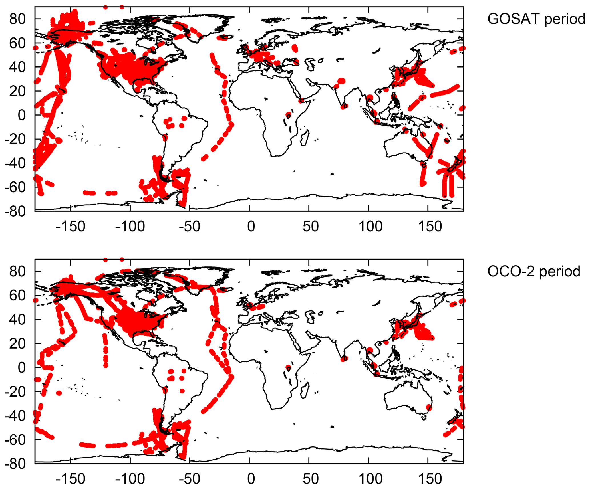
Figure 1Location of the aircraft measurements used in the free troposphere for the two verification periods. Note that the two periods overlap by 22 months, so that many data appear on both maps.

2.5 Poor man's inversion

In order to put the differences between inversion simulations and aircraft measurements into perspective, we compare them to an inversion that only assimilated the annual global growth rate of CO₂. This baseline, called “the poor man's inversion” by Chevallier et al. (2009), adjusts prior natural fluxes over land in order to fit the annual trend of globally averaged marine measurements (http://www.esrl.noaa.gov/gmd/ccgg/trends/, last access: 10 January 2019) multiplied by a conversion factor (2.086 GtC ppm⁻¹, from Prather, 2012) when combined with prior ocean and fossil fuel fluxes. The correction to the natural land fluxes is made proportional to the prior error standard deviations assigned within a given inversion system. In the case of the CAMS system here, the prior error standard deviations are themselves proportional to a climatology of heterotrophic respiration fluxes simulated by a vegetation model, with a ceiling of 4 gC m⁻² d⁻¹. This simple approach is not Bayesian because prior error correlations are ignored, but it still allows transport models to fit atmospheric data with less bias than its prior fluxes because it closes the carbon budget in a plausible way.

Over the ocean and for the fossil fuel emissions, we choose the same prior fluxes as for the six Bayesian inversions (Landschützer et al., 2017; Crippa et al., 2016; Le Quéré et al., 2018, see Sect. 2.2). However, we choose more informed natural fluxes over land than for the Bayesian inversions: rather than leaving the inversion fully free to locate the annual land sinks (see Sect. 2.2), we use a simulation of a dynamic global vegetation model that accounts for land use, climate and CO₂ history (simulation ORCHIDEE-trunk in Le Quéré et al., 2018). When multiplied by 2.086 GtC ppm⁻¹, this combination of prior fluxes already fits the annual trend of globally averaged marine measurements with a root-mean-square difference of 0.3 ppm a⁻¹, By construction, the poor man's adjustment brings these annual global differences to zero.

For the comparison of the poor man's inversion with aircraft measurements, we use LMDz5A. We start the poor man's simulation on 1 January 2000 from a 3-D prior initial state of CO₂. We then add an offset to the simulation so that its mean bias with respect to NOAA's surface measurements at the South Pole Observatory (Cooperative Global Atmospheric Data Integration Project, 2018) over the 2010–2017 period is zero. This offset addresses the uncertainty of the initial state and the uncertainty of the 2.086 GtC ppm⁻¹ conversion factor.

3.1 Principle

We build an ensemble of six Bayesian inversions using the inversion system from Sect. 2.2, the two transport model versions from Sect. 2.1 and the three observation datasets from Sect. 2.3. The assimilation periods differ (Sect. 2.2), but the prior fluxes and the prior error model are the same. For each inversion, the posterior model simulation statistically fits its own assimilated data well within their 1σ uncertainty. Note that the surface-based inversion with LMDz5A is exactly the same as the CO₂ inversion product version 18r1 of CAMS that was released in November 2018 (http://atmosphere.copernicus.eu/, last access: 21 November 2019). In the figures, we will refer to the surface-based inversions by the generic name “SURF” for simplicity.

We first present the carbon budget estimates. We choose to look at fluxes at the annual scale only, knowing that the inferred interannual variability is completely driven by the assimilated observations over land (because prior natural fluxes over land are zero on annual average for the Bayesian inversions, see Sect. 2.2). As we will see, it is relatively large. Except at the global scale, capturing the interannual variability well is particularly challenging because its estimation accumulates all errors made throughout the seasonal cycle.

Then we compare the inversion performance vis-à-vis the aircraft measurements of Sect. 2.4, to the performance of the poor man's inversion of Sect. 2.5. This comparison is made for two periods (Sect. 2.4). For each of them, we will only consider the inversions that cover the window completely, which means that the GOSAT-based (or OCO-2-based) inversions will not be used in the results for the “OCO-2 period” (or “GOSAT period”). The projection of the inversion fluxes onto the space of the aircraft-measured variables (mole fractions) is made by the same LMDz model version that was used in the inversion. Thus, we are consistent with the way the inversion system distributes the well-constrained total mass of carbon in the atmosphere and we avoid error compensations between the version used in the assimilation and the one used in the evaluation. The model is directly sampled at measurement time and space, without any interpolation: the grid cell value is used as the simulated value for the verification data.

3.2 Annual budgets

The time series of the annual natural carbon budgets at several very broad scales are displayed in Fig. 2 for the period between 2004 and 2017: the globe, the northern or southern extratropics, and the tropics with lands and oceans either separated or combined. At this scale, the influence of the transport model version is hardly distinguishable (coloured solid lines vs. coloured dashed lines). The poor man's inversion (black dashed lines) locates the land sink mostly in the northern extratropics but also in the tropics (consistent with its prior information shown in Fig. 8 of Le Quéré et al., 2018), whereas the six Bayesian inversions put it more in the northern extratropics (starting from a null prior on annual average). All approaches converge towards near-neutral southern extratropical lands (that represent a relatively small surface area). Over the oceans, the surface-based inversions vary little from the prior (which is equal to the poor man's estimate there), but the GOSAT-based inversions reduce the ocean sink by about 0.5 GtC a⁻¹ in 2015; the OCO-2-based inversions increase it by up to 1 GtC a⁻¹. We recall that years 2015 and 2016 correspond to a strong El Niño event associated with a large CO₂ growth rate (e.g. Malhi et al., 2018 and references therein). The GOSAT inversions seem to underestimate the beginning of this anomaly (Fig. 2a), and to attribute it to the southern extratropical oceans rather than to the tropical lands like the other inversions. OCO-2-based fluxes are close to the surface-based fluxes, except for the increased ocean sink (which appears to be regularly spread between the three bands). The OCO-2-based and surface-based growth rates are very similar, but do not fully overlap with the poor man's fluxes because they do not fully agree with NOAA's estimates, in particular in 2016 when they diagnose a smaller rate (by 0.25 ppm a⁻¹ if we use the 2.086 GtC ppm⁻¹ conversion factor).

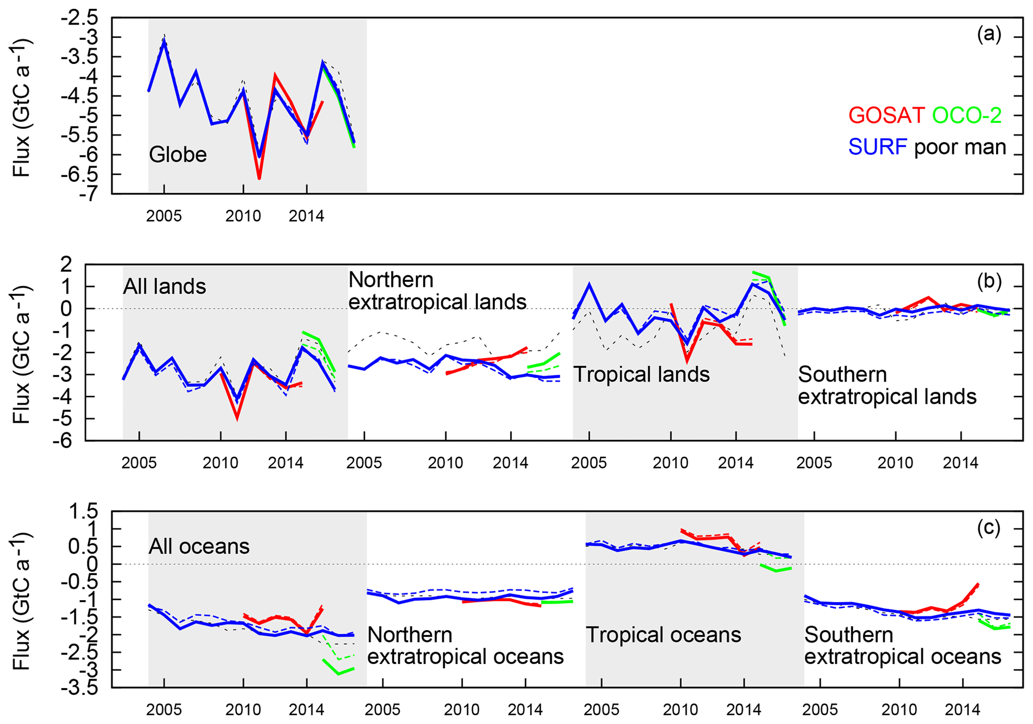
Figure 2Time series of inferred natural CO₂ annual flux (without the prescribed fossil fuel emissions) between 2004 and 2017, averaged over the globe or over all lands or oceans. In the case of lands and oceans three broad latitude bands are also defined: northern extratropics (north of 25^∘ N), tropics (within 25^∘ of the Equator), and southern extratropics (south of 25^∘ S). Inversions with LMDz5A (LMDz6A) are shown using continuous (dashed) coloured lines. In the sign convention, positive fluxes correspond to a net carbon source into the atmosphere. The last year of the GOSAT inversions (2016) is not represented because it is less constrained at the end by the lack of 2017 retrievals here. Note that the prior fluxes are zero over land at this temporal scale (see Sect. 2.2) and that they are equal to the “poor man” curve over the ocean (see Sect. 2.5).

Download

Figures 3 and 4 focus on the Bayesian inversion results at the scale of the 22 regions of the TransCom 3 experiment (Gurney et al., 2002): 11 regions over land and 11 regions over the oceans that together tile the whole globe. At this scale, the impact of the choice of the LMDz version appears: LMDz6A induces slightly less year-to-year variability for the surface-based inversion for some years (see the 2010s for the Europe region, the last couple of years for the Eurasian temperate region or the full time series for the North Atlantic temperate region), and the two model versions can yield different baselines (see the North American temperate and South American temperate regions, or the three Atlantic regions). The two GOSAT-based inversions show larger year-to-year variability than the other inversions. The OCO-2-based inversions broadly agree with the surface-based inversions for the temporal variability of the fluxes in most regions (North American boreal, Southern Africa, Eurasian boreal, Tropical Asia, Europe) but there are noticeable differences in the North American temperate, South American tropical, South American temperate and Australia regions. While being clearly distinct from the inversion prior fluxes (that are zero on annual average over land), and from the GOSAT-based fluxes, we note the agreement of the two OCO-2-based inversions with the 6A SURF inversion and the poor man's fluxes (that are informed by an up-to-date bottom-up simulation) in the two boreal regions, despite the lack of OCO-2 data there during half of the year as a consequence of insufficient insolation (see e.g. Deng et al., 2014). The main differences between inversions OCO-2 and SURF over the ocean are the North Pacific temperate and Southern Ocean regions.

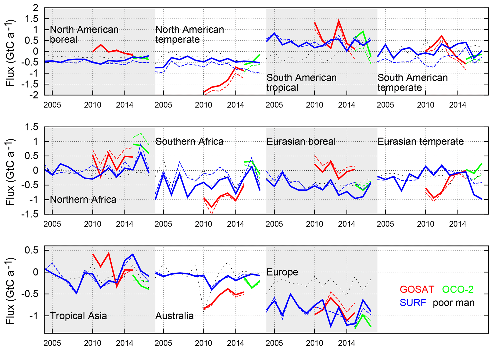
Figure 3Time series of inferred natural CO₂ annual flux (without the prescribed fossil fuel emissions) between 2004 and 2017, averaged over TransCom 3 land regions. Inversions with LMDz5A (LMDz6A) are shown using continuous (dashed) coloured lines. In the sign convention, positive fluxes correspond to a net carbon source into the atmosphere. The last year of the GOSAT inversions (2016) is not represented because of likely edge effects. Note that the prior fluxes are zero over land at this temporal scale (see Sect. 2.2).

Download

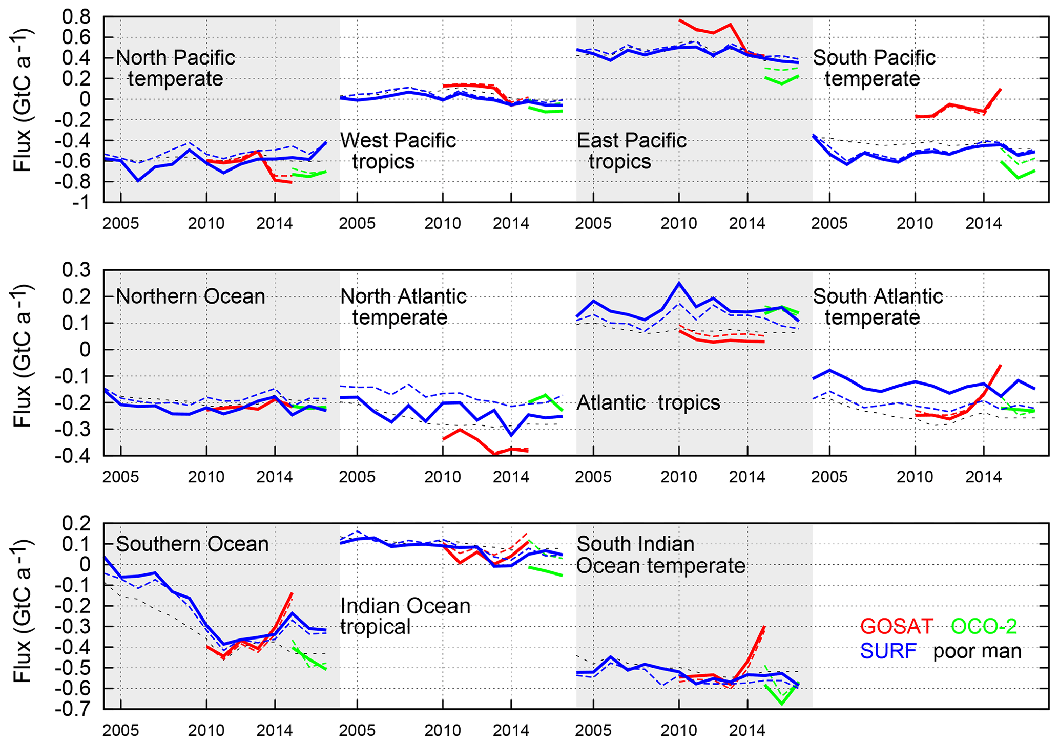
Figure 4Same as Fig. 3 but for oceanic regions. Note that the prior fluxes over the ocean are equal to the “poor man” curve (see Sect. 2.5).

Download

Figure 5 compares the difference between fluxes estimated by assimilating either OCO-2-based or surface-based data within LMDz6A to the posterior uncertainty diagnosed from the Bayesian system (Chevallier et al., 2007) for the surface-based inversion. For all regions discussed so far, this difference is usually within the Bayesian uncertainty standard deviation (but reaches up to 2.6 times this quantity in northern Africa for 2015), which means that the difference between the two flux estimates at this scale is mostly not statistically significant.

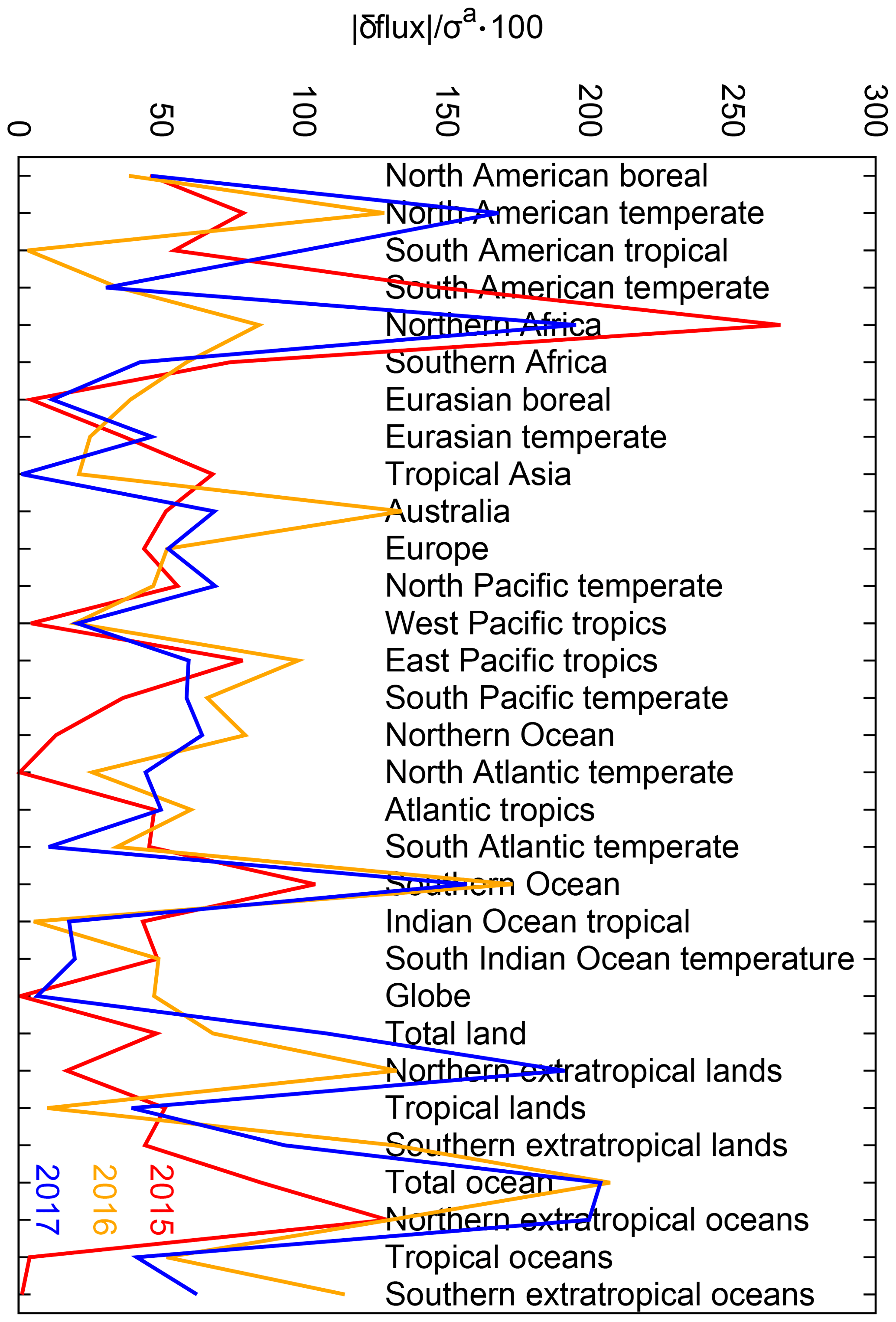
Figure 5Ratio of the absolute difference (δ flux) between the OCO-2-based annual fluxes and the surface-based annual fluxes to the Bayesian posterior flux uncertainty for the surface-based fluxes (σ^a), in percent, for the years 2015, 2016 and 2017. Both inversions correspond to LMDz6A.

Download

Figure 6 further zooms in to the pixel-scale for the year 2015, a year that is common between all inversions. Only the LMDz5A results for the satellite-based inversions are shown. For the two surface-based inversions, the change of transport model leaves the flux patterns generally unchanged but slightly modulates their amplitude. In contrast, the two satellite-based inversions show more differences in the flux pattern. They suggest large flux gradients in southern Africa and South America: the fluxes are similar for GOSAT and OCO-2 in Africa, with a large sink in the tropical evergreen forests and large sources around these same forests, whereas they are different in America with a source over the tropical evergreen forests for GOSAT and over a northeast corner for OCO-2. The broad flux patterns in the lands of the Northern Hemisphere are similar between the four maps, but OCO-2 has flux gradients closer to SURF than to GOSAT in America while the opposite is seen in Southeast Asia. The tropical ocean outgassing region reduces with OCO-2 and expands to the south with GOSAT.

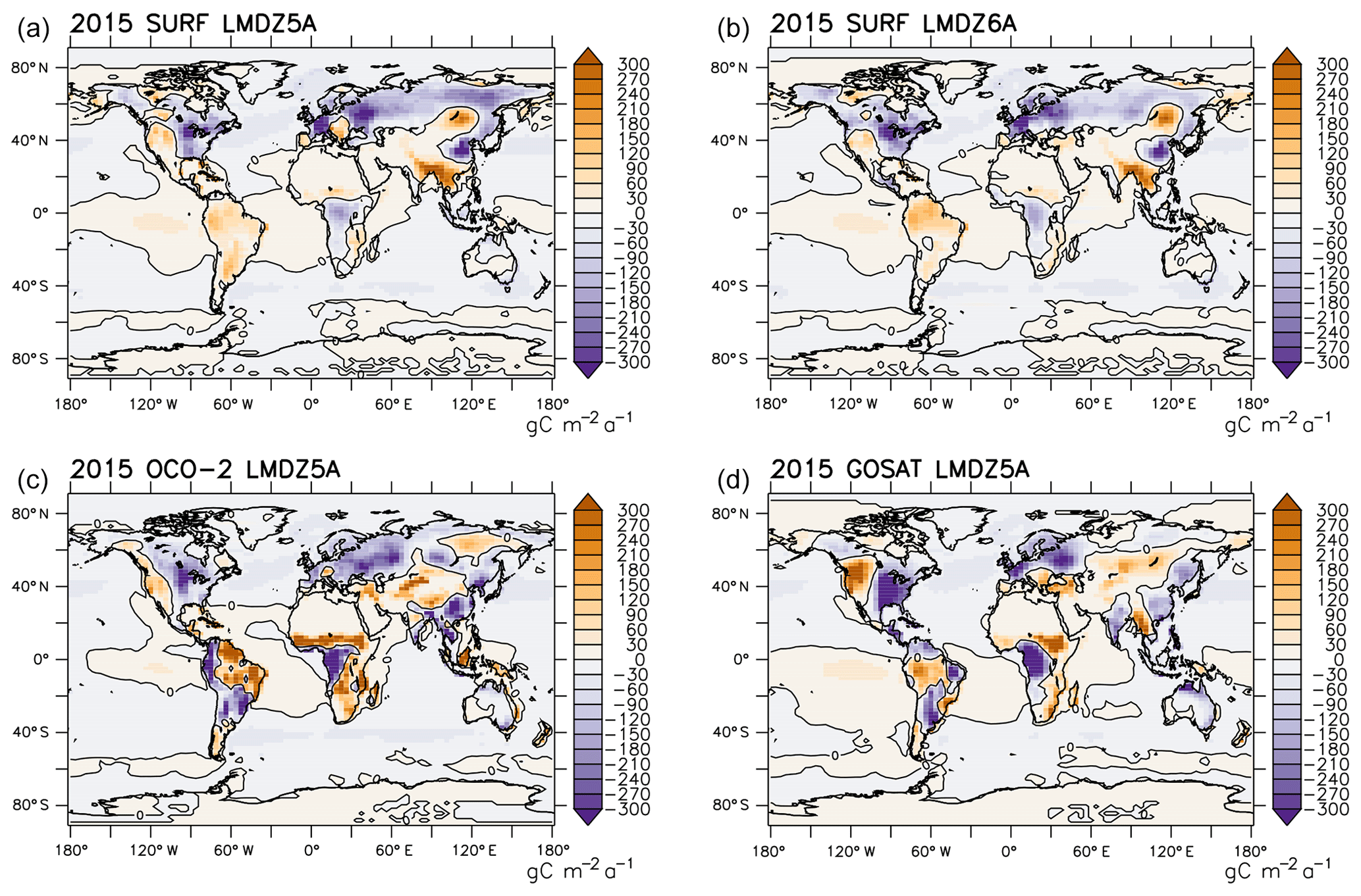
Figure 6Grid-point budget of the natural CO₂ fluxes for the year 2015. In the sign convention, positive fluxes correspond to a net carbon source into the atmosphere.

3.3 Differences with aircraft data

Figure 7 presents the statistics of model-minus-measurement differences per measurement programme for the GOSAT period. Note that the data number varies by several orders of magnitude among the programmes: there are a few hundred samples for most of the 37 programmes, but a few thousand for CALNEX2010, KORUS-AQ, ORCAS, SGP and ATom, a few tens of thousands for ACT, DC3, DISCOVER-AQ, GSFC, HIPPO, SEAC4RS and SONGNEX2015, and 900 000 for CONTRAIL. Obviously, many measurements may fit into a single time–space block of the global transport model. We will only discuss bias differences larger than 0.15 ppm (i.e. above the calibration uncertainty of the aircraft data, see Sect. 2.4) and those that are statistically significant at the 0.05 level, as reported in the figure. The computation of the significance level is made using an unpaired t test when comparing inversion results that assimilated different data (we assume that changing the assimilated data makes the inversion results independent), and using a paired t test when comparing inversion results that assimilated the same data (we assume that inversion results in which only the transport model varies are dependent). In practice, changing the independency assumption only affects the detail of the significance level results, but not the overall picture.

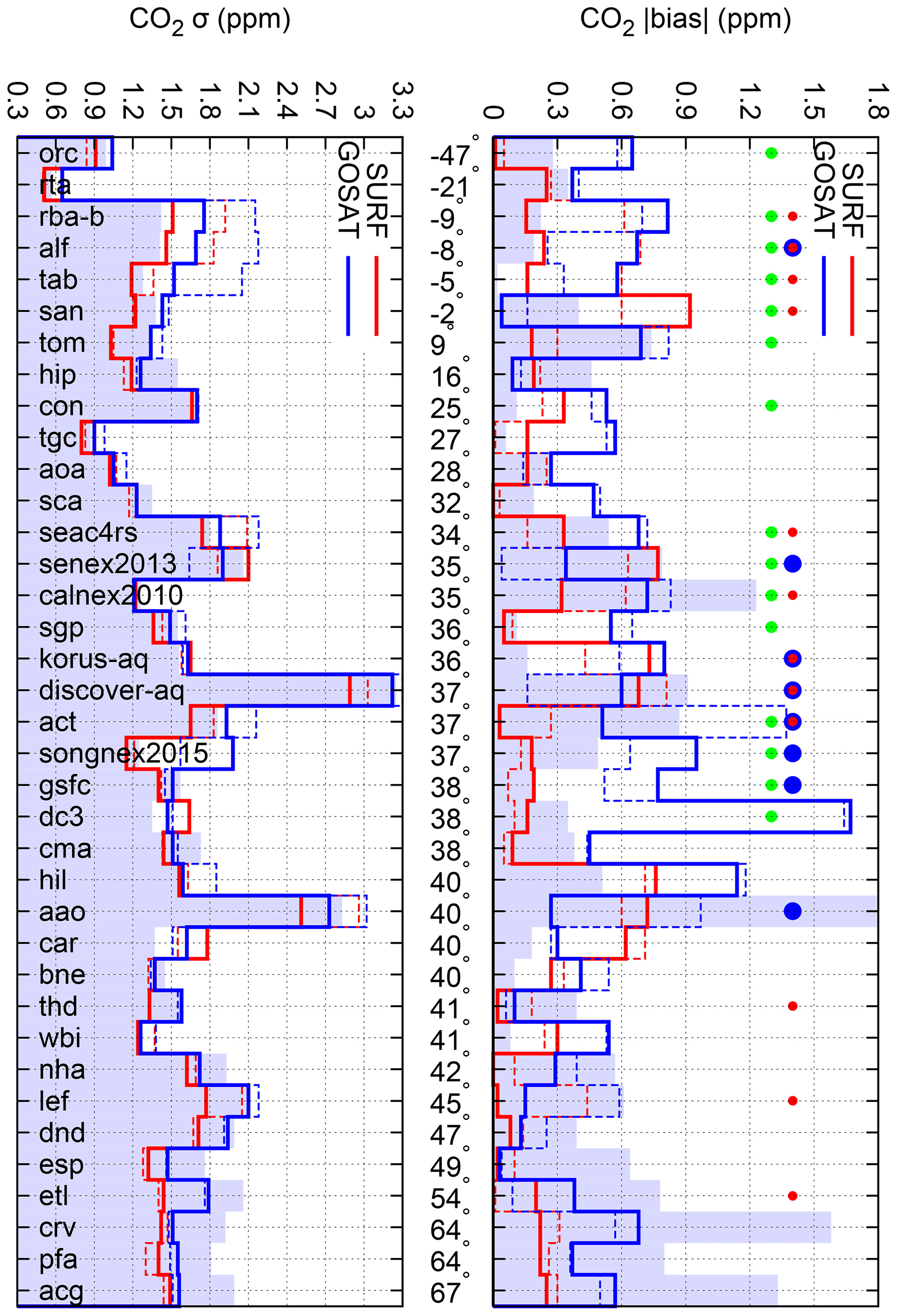
Figure 7Model-minus-observation absolute differences and standard deviations over the GOSAT period per measurement programme for the surface-based inversion (SURF, red line), the GOSAT-based inversion (GOSAT, blue line) and the poor man's inversion (shaded area). Inversions with LMDz5A (LMDz6A) are shown using continuous (dashed) coloured lines. The number of measurements per site, campaign or programme varies between 113 (BNE) and 901 846 (CON). The programme definitions are given in Table 1. They are ranked by increasing mean latitude (north is on the right), irrespective of their latitudinal coverage (which is large at several tens of degrees for ORC, TOM, HIP and CON). These mean latitudes are shown in the middle of the panel. For each programme, a green circle appears in the upper panel if the difference between the GOSAT bias and the SURF bias using LMDz5A is statistically significant (see the main text for a definition) and exceeds 0.15 ppm. Similarly, a red (blue) circle indicates that the difference between LMDz5A and LMDz6A for SURF (GOSAT) is statistically significant and exceeds 0.15 ppm.

Download

Comparing solid and dotted lines, we see no benefit of LMDz6A vs. LMDz5A, as version 6A increases the absolute bias of SURF for eight programmes (three in Brazil – RBA-B, ALF and TAB, as well as CALNEX2010, DISCOVER-AQ, ACT, THD and LEF) and improves it for four programmes (the fourth Brazilian site – SAN , as well as SEAC4RS, KORUS-AQ and ETL). There is no obvious consistency between the changes brought by LMDz6A to the surface-based inversion and those brought to the GOSAT-based inversion. For SAN and SENEX2013, the two surface-based inversions have larger absolute biases than the GOSAT-based inversions, but perform better for 11 other sites. The poor man's inversion shows the worse biases north of 45^∘ N, but usually performs better than the GOSAT-based inversion in the Southern Hemisphere, likely helped by the tuning with the South Pole Observatory data. Between the Equator and 45^∘ N, the relative performance of the poor man's inversion is uneven but it is usually not as good as SURF. In terms of standard deviation (bottom row of Fig. 7), the surface-based inversions have the smallest values.

There are 26 aircraft programmes in the OCO-2 period. They challenge SURF a little less (Fig. 8) than for the GOSAT period: apart from INPE, GSFC and KORUS-AQ (12 % of the programmes), all absolute SURF biases are less than 0.45 ppm, while seven programmes (19 % of the programmes, i.e. SAN, SENEX2013, KORUS-AQ, DISCOVER-AQ, HIL, AAO and CAR) previously exceeded this threshold. The relatively close flux estimates between SURF and OCO-2 inversions (Figs. 2–6) translate into relatively close performance compared with the aircraft programmes. SURF performs better than OCO-2 for INPE and ACT in terms of biases, and worse for GSFC and KORUS-AQ. The poor man's simulation has less skill than in the GOSAT period: it performs much worse than the surface-based and the OCO-2-based inversions in the Northern Hemisphere, and is comparable or better in the Southern Hemisphere. If we combine all measurements, the root-mean-square difference for the OCO-2-based and the surface-based inversions only varies between 1.51 and 1.56 ppm. Note that 39 % of these data are from CONTRAIL, a programme that spreads over all continents. If we only take CONTRAIL data, the root-mean-square difference for the OCO-2-based and the surface-based inversions still only varies between 1.60 and 1.67 ppm, which tends to indicate that this result is not biased towards features that are specific to one region. The standard deviations are comparable between the OCO-2-based inversions and the surface-based inversions. LMDz6A improves the SURF biases for KORUS-AQ and degrades them for three other programmes (INPE, LEF and ETL). This lack of improvement also appears for OCO-2 (degradation at INPE, KORUS-AQ and ABOVE). The statistics for four programmes (ORCAS, KORUS-AQ, ACT and SONGNEX2015) are directly comparable between the two periods because the corresponding data are complete in both periods: in all four programmes OCO-2 performs better than GOSAT.

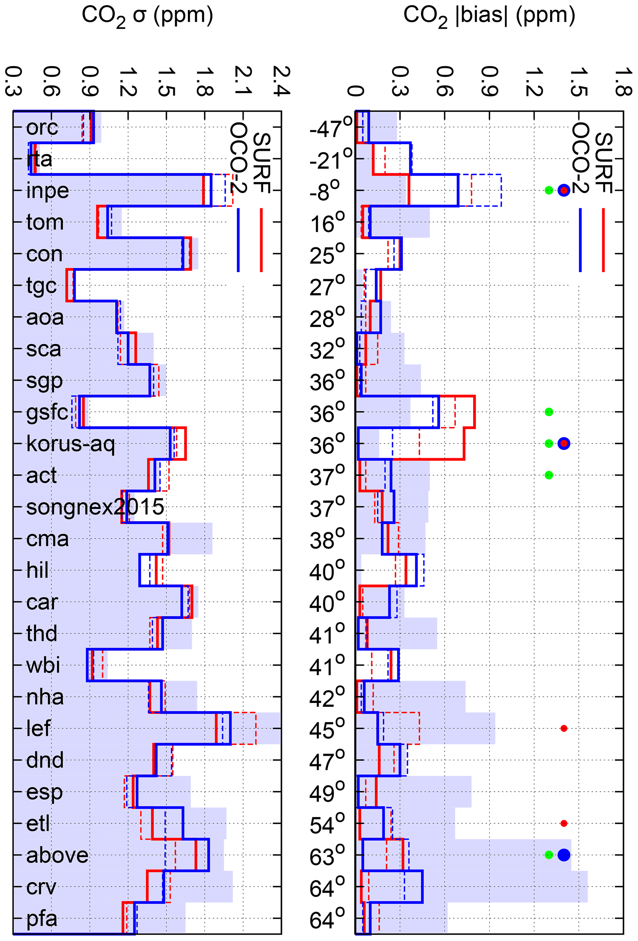
Figure 8Same as Fig. 7 for the OCO-2 period. The number of measurements per programme varies here between 133 (CRV) and 211 358 (CON).

Download

Figure 9 reformulates the bias statistics of Fig. 8 on a map of the differences between the absolute biases of the OCO-2 and SURF inversions. As for the programme biases, some points are more robust than others (due to varying amount of data), but there is some large-scale coherence, with better performance of SURF in the Southern Hemisphere (as could already be seen in Figs. 7 and 8) and in the central and eastern US, whereas OCO-2 yields smaller biases in the Northern Hemisphere subtropics and Europe. Other parts of the globe are less consistent such as the western Pacific edge or boreal America.

Figure 9Difference between the model-minus-observation absolute differences in 10^∘ moving windows (a). Negative (positive) values denote areas where the OCO-2-based inversion has smaller (larger) biases than the surface-based inversion. Both inversions use LMDz5A. Panel (b) gives the number of data that contribute to the bias computation in each 10^∘ moving window. Biases are only computed in the windows where there are more than 100 measurements.

3.4 Pixel attribution

Liu and Bowman (2016) proposed a method to quantify the impact of flux changes over the globe on the corresponding change in the mean squared error (MSE) of the transport model simulation with respect to n independent measurements. They demonstrated it in the case of the flux changes from their prior values to their posterior values within the approximations of a linear transport model M (including the sampling operator at the measurement time and location) and of an unchanged initial state of CO₂. It is actually valid for other types of changes within an inversion, provided they respect the tangent linear hypothesis for the transport model. The change in the MSE (δMSE) is expressed as a finite sum of terms. There is one term for each element i of the inversion control vector (i.e. a CO₂ flux at a given time and location, or some part of the 3-D initial state of CO₂):

Term i is the product of the corresponding change in the control vector (i.e. a scalar δf_i), times the corresponding row of the transpose of the linear model M, times (dot product here) the vector of the sum of the differences between the two model simulations (one, c₁, before the change in the control vector and one, c₂, after the change) and all verification measurements (δc₁+δc₂, both vectors with dimension n). Interestingly, the second product in this formula can be calculated by the adjoint code of the transport model, if it exists, which is the case for LMDz (Sect. 2.2). Further detail is given in Liu and Bowman (2016).

We apply this approach to interpret the difference between the OCO-2-based and the surface-based inversions using LMDz5A. The overall MSE is very similar between both (1.5² ppm²), but the relative performance still varies in space and time (Figs. 8, 9) and we hope to extract some further insight into the relative merits of each dataset. In practice, we compute δc₁+δc₂ using the LMDz model linearised around the inversion prior simulation in order to respect the underlying hypothesis. However, some inconsistencies for the initial state of CO₂ could not be completely removed between δc₁ and δc₂ due to the different starting date of each inversion. The map of the sum of all contributions of the flux changes δf_i (from the surface-based inversion to the OCO-2-based inversion) at a given pixel to the change in MSE (δMSE) is presented in Fig. 10. Positive values occur when the OCO-2-based fluxes increase the MSE relative to the surface-based fluxes. This happens in the western contiguous US, northeastern South America, western Europe, Turkey, the West Siberian Plain and eastern Siberia. Contributions to reduce the MSE (negative values) are mostly in Alaska and the eastern contiguous US, western South America, southern Africa, South and Southeast Asia, and Indonesia. No noticeable contribution is seen over the ocean, where OCO-2 retrievals have not been assimilated. By construction, regions that are not well observed downstream by aircraft have lesser contributions, like in Africa. This feature makes the relative magnitude of the patterns among each other not very informative regarding the flux quality. Therefore, we will pay more attention to the sign of the dominant patterns.

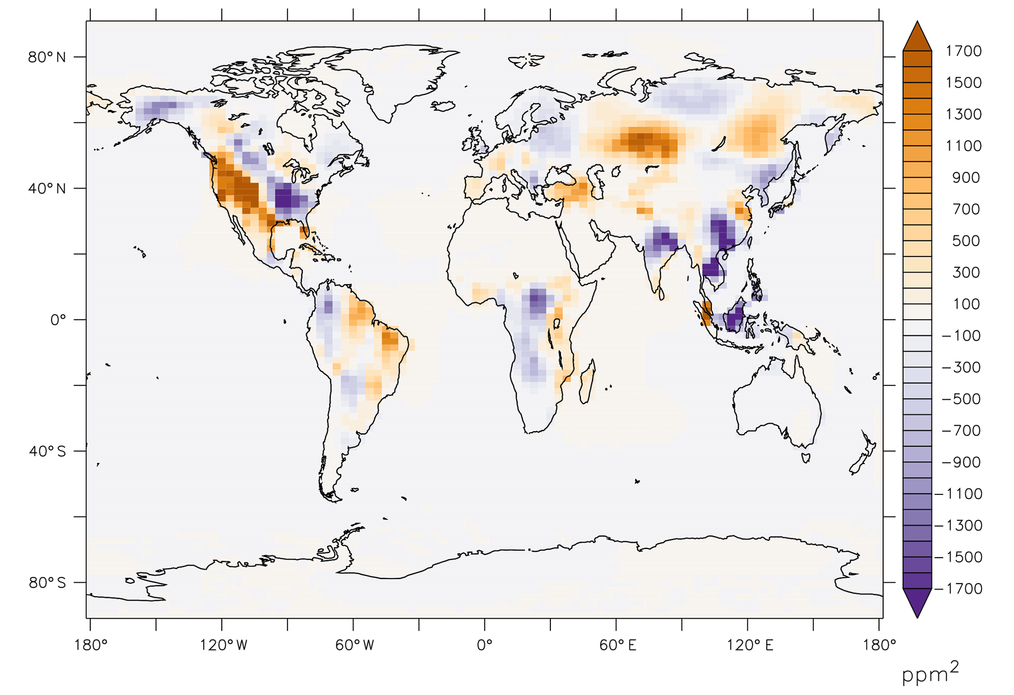
Figure 10Contribution of the grid-point flux changes to the change in the variance of CO₂ model–measurement differences between the OCO-2-based inversion and the surface-based inversion (variance of the former minus variance of the latter), in parts per million squared. Both inversions use LMDz5A. Note that the fluxes themselves are illustrated in Fig. 6a and c.

The map in Fig. 9, which refers to differences in absolute biases within moving windows, is, in principle, not directly comparable with Fig. 10, which refers to MSEs. However, bias changes are much larger than standard deviation changes (Fig. 8) which makes the map of root-mean-square errors (RMSEs, not shown) very similar to Fig. 9. Differences between the patterns in Fig. 9 in the space of free-tropospheric mole fractions and those in Fig. 10 in the space of fluxes are linked to the way CO₂ is transported between the surface and the free troposphere. Dominating westerlies outside the tropics bring the positive flux contributions in Fig. 10 to the west of the positive RMSE variations in Fig. 9, like from the western to the eastern US, or, at a much larger scale, from Eurasia to Alaska. Similarly, negative flux contributions from the eastern US induce negative RMSE variations in the central North Atlantic Ocean, and tropical easterlies link the negative flux contributions from southern Africa to the negative RMSE variations in the tropical Atlantic Ocean. The distance between the flux signal and the free-tropospheric signal implies an important role for the transport model in attributing the latter to the former; therefore, these patterns should be considered with caution, as is the case for inversion systems in general.