the Creative Commons Attribution 4.0 License.
the Creative Commons Attribution 4.0 License.
 | 11 Nov 2019
Technical note: Reanalysis of Aura MLS chemical observations
Quentin Errera
Simon Chabrillat
Yves Christophe
Jonas Debosscher
Daan Hubert
William Lahoz
Michelle L. Santee
Masato Shiotani
Sergey Skachko
Thomas von Clarmann
Kaley Walker
This paper presents a reanalysis of the atmospheric chemical composition from the upper troposphere to the lower mesosphere from August 2004 to December 2017. This reanalysis is produced by the Belgian Assimilation System for Chemical ObsErvations (BASCOE) constrained by the chemical observations from the Microwave Limb Sounder (MLS) on board the Aura satellite. BASCOE is based on the ensemble Kalman filter (EnKF) method and includes a chemical transport model driven by the winds and temperature from the ERA-Interim meteorological reanalysis. The model resolution is 3.75∘ in longitude, 2.5∘ in latitude and 37 vertical levels from the surface to 0.1 hPa with 25 levels above 100 hPa. The outputs are provided every 6 h. This reanalysis is called BRAM2 for BASCOE Reanalysis of Aura MLS, version 2.
Vertical profiles of eight species from MLS version 4 are assimilated and are evaluated in this paper: ozone (O3), water vapour (H2O), nitrous oxide (N2O), nitric acid (HNO3), hydrogen chloride (HCl), chlorine oxide (ClO), methyl chloride (CH3Cl) and carbon monoxide (CO). They are evaluated using independent observations from the Atmospheric Chemistry Experiment Fourier Transform Spectrometer (ACE-FTS), the Michelson Interferometer for Passive Atmospheric Sounding (MIPAS), the Superconducting Submillimeter-Wave Limb-Emission Sounder (SMILES) and N2O observations from a different MLS radiometer than the one used to deliver the standard product and ozonesondes. The evaluation is carried out in four regions of interest where only selected species are evaluated. These regions are (1) the lower-stratospheric polar vortex where O3, H2O, N2O, HNO3, HCl and ClO are evaluated; (2) the upper-stratospheric–lower-mesospheric polar vortex where H2O, N2O, HNO3 and CO are evaluated; (3) the upper troposphere–lower stratosphere (UTLS) where O3, H2O, CO and CH3Cl are evaluated; and (4) the middle stratosphere where O3, H2O, N2O, HNO3, HCl, ClO and CH3Cl are evaluated.
In general BRAM2 reproduces MLS observations within their uncertainties and agrees well with independent observations, with several limitations discussed in this paper (see the summary in Sect. 5.5). In particular, ozone is not assimilated at altitudes above (i.e. pressures lower than) 4 hPa due to a model bias that cannot be corrected by the assimilation. MLS ozone profiles display unphysical oscillations in the tropical UTLS, which are corrected by the assimilation, allowing a good agreement with ozonesondes. Moreover, in the upper troposphere, comparison of BRAM2 with MLS and independent observations suggests a positive bias in MLS O3 and a negative bias in MLS H2O. The reanalysis also reveals a drift in MLS N2O against independent observations, which highlights the potential use of BRAM2 to estimate biases between instruments. BRAM2 is publicly available and will be extended to assimilate MLS observations after 2017.
- Article
(9383 KB) - Full-text XML
-
Supplement
(7177 KB) - BibTeX
- EndNote


An atmospheric reanalysis is an estimation of the past atmospheric state using the information provided by an atmospheric numerical model and a set of observations combined by a data assimilation system. Historically, atmospheric reanalyses have been produced by meteorological centres and upper-level products consisting mainly of temperature, winds, humidity, geopotential height and ozone. They have been used “to understand atmospheric processes and variability, to validate chemistry-climate models and to evaluate the climate change” (Fujiwara et al., 2017).
With the increase in the number of chemical observations from satellites and the advent of chemical data assimilation systems (Lahoz and Errera, 2010), several reanalyses of the atmospheric chemical composition have been produced, most recently, the Copernicus Atmospheric Monitoring Service (CAMS) reanalysis (Inness et al., 2019) and the Tropospheric Chemical Reanalysis (TCR; Miyazaki et al., 2015). These two reanalyses focus mainly on the tropospheric composition with few assimilated species in the stratosphere (ozone in both cases and nitric acid in TCR). With a focus on the stratosphere, Errera et al. (2008) presented an assimilation of measurements from the Michelson Interferometer for Passive Atmospheric Sounding (MIPAS) but limited to only 18 months and to two species (ozone and nitrogen dioxide). Also focusing on the stratosphere, Viscardy et al. (2010) made an assimilation of observations from the Microwave Limb Sounder (MLS) on board the UARS satellite between 1992 and 1997, but again also limited to ozone.
The second generation of MLS (Waters et al., 2006), on board the Aura satellite, has been operating since August 2004 and is still measuring at the time of writing. It measures vertical profiles of around 15 chemical species from the upper troposphere to the mesosphere with a high stability in terms of spatial and temporal coverage (SPARC, 2017) and data quality (Hubert et al., 2016). A subset of the Aura MLS (hereafter simply denoted MLS) constituents has been assimilated in near-real time (NRT) since 2009 by the Belgian Assimilation System for Chemical ObsErvations (BASCOE) in order to evaluate the stratospheric products from CAMS (Lefever et al., 2015). The BASCOE MLS analyses have also been used by the World Meteorological Organization (WMO) Global Atmospheric Watch (GAW) programme to evaluate the state of the stratosphere during polar winters (e.g. Braathen, 2016).
Chemical analyses of the stratosphere have additional potential applications. They could be used to evaluate chemistry–climate models. Usually, this is done with climatologies, which are based on zonal mean monthly means of observations (Froidevaux et al., 2015; Davis et al., 2016; SPARC, 2017) and thus affected by uncertainties due to the irregular sampling of the instruments, especially those with a low spatial coverage such as solar occultation instruments (Toohey and von Clarmann, 2013; Millán et al., 2016). Chemical analyses could also be used to study the differences between instruments using the reanalysis as a transfer function (Errera et al., 2008). Moreover, chemical analyses could provide an internally consistent set of species to enable scientific questions to be addressed more completely than with measurements alone. Although not addressed in this paper, the BASCOE data assimilation system provides the complete set of chlorine species while only a few of them are assimilated (hydrogen chloride and chlorine oxide), which can be useful to analyse polar processing studies. Finally, chemical analyses can be used to set model boundary conditions, e.g. the lower stratosphere in the estimation of carbon monoxide emissions with the inversion method (Müller et al., 2018).
On the other hand, the BASCOE NRT analyses have several shortcomings, in particular the versions of the BASCOE system and of the MLS observations have changed several times since the start of the service. This paper thus presents a reanalysis of Aura MLS using one of the latest versions of BASCOE and MLS and covers the period August 2004–December 2017. Eight MLS species are assimilated: ozone (O3), water vapour (H2O), nitrous oxide (N2O), nitric acid (HNO3), hydrogen chloride (HCl), chlorine oxide (ClO), methyl chloride (CH3Cl) and carbon monoxide (CO). Although several other satellite instruments also measured vertical profiles of chemical stratospheric species during that period and beyond (see, e.g. SPARC, 2017), these observations were not assimilated in order to avoid the introduction of spurious discontinuities such as in ERA-Interim upper-stratospheric temperature (Simmons et al., 2014, their Fig. 21).
The reanalysis presented in this paper is named the BASCOE Reanalysis of Aura MLS, version 2 (BRAM2). Version 1 of the reanalysis, BRAM1, was released in 2017 but not published. This paper is organized as follows. Section 2 presents the MLS observations assimilated in BRAM2 and the independent observations used for its validation. Section 3 presents the BASCOE system and its configuration for BRAM2. The method to intercompare BRAM2 with the observations is described in Sect. 4. The evaluation of BRAM2 is presented in Sect. 5, including a summary. The conclusions are given in Sect. 6.
2.1 The assimilated MLS observations
The BRAM2 reanalysis is based on the assimilation of observations taken by the Microwave Limb Sounder (MLS; Waters et al., 2006) operating on NASA’s Aura satellite. MLS measures vertical profiles of around 15 chemical species. For BRAM2, the following species have been assimilated: O3, H2O, N2O, HNO3, HCl, ClO, CO and CH3Cl. Other MLS species are not considered because, with the exception of OH, they either are available over only a limited vertical range or require substantial averaging prior to use in scientific studies. OH profiles have not been assimilated because modelled OH is more controlled by the atmospheric conditions (e.g. temperature) and the state of long-lived species (in particular H2O) than by its initial conditions. While a similar situation holds for ClO in the middle stratosphere (here the long-lived species would be HCl), this is not the case in conditions of chlorine activation, such as in the lower-stratospheric polar vortex.
MLS was launched in July 2004 and provided its first profiles in August of that year. At the time of writing, the instrument is still in operation despite showing some ageing degradation. Around 3500 vertical profiles are delivered every day, measured during daytime and night-time. In this paper, we have used version 4.2 (v4) of MLS profiles as described in Livesey et al. (2015, denoted L2015 hereafter). Each MLS profile is checked before assimilation according to the recommendations given in L2015. Profiles are only assimilated in the vertical range of validity given in L2015 and reported in Table 4. Profiles, or part of them, are discarded if the “estimated precision”, “quality”, “convergence” and “status” are outside the ranges given in L2015. In particular, this screening discarded profiles contaminated by clouds, mainly for O3, HNO3 and CO. ClO profiles show biases at and below 68 hPa and have been corrected according to L2015.
MLS O3 profiles exhibit vertical oscillations in the tropical tropopause layer (TTL; see L2015; Yan et al., 2016). Although improvements have been made in v4 compared to previous versions, this problem has not been eliminated (see Sect. 5.4). The BASCOE chemistry transport model (CTM) also suffers from an ozone deficit around 1 hPa that assimilation cannot correct. This led us to assimilate MLS O3 observations only at altitudes below (i.e. pressure greater than) 4 hPa (see Sect. 3.1).
In MLS v4, the standard product for N2O is derived from radiances measured by the 190 GHz radiometer. Previous MLS data versions used the 640 GHz radiometer, which provided slightly better quality, but this product ceased to be delivered after August 2013 because of instrumental degradation in the band used for that retrieval. For BRAM2, the 190 GHz N2O product is assimilated for the whole period to avoid discontinuity when switching between different products.
CO profiles suffer from several artefacts as reported by L2015. They show a positive systematic error of 20 %–50 % in the mesosphere and a negative systematic error of 50 %–70 % near 30 hPa. Between 1 and 0.1 hPa, profiles are rather jagged. There is also a tendency toward negative values below levels where CO abundances are large, especially in the polar vortex when high concentrations of CO descend to the mid-stratosphere. No corrections have been applied to resolve these artefacts because none are recommended by the MLS team. Although BRAM2 has assimilated MLS CO within its recommended vertical range of validity (0.0046–215 hPa), BRAM2 CO will be evaluated only where CO is relevant for stratospheric dynamics, i.e. in the polar vortex above 10 hPa and in the upper troposphere–lower stratosphere (UTLS).
The error budget of each species has also been estimated by L2015. This information is given as uncertainty profiles of accuracy and precision, and it will be used in the validation of the BRAM2 products. Note that L2015 provides 2σ accuracy and 1σ precision. In this paper, we are using the 1σ uncertainties for both the accuracy and precision.
2.2 Independent observations used for validation
2.2.1 ACE-FTS
The Atmospheric Chemistry Experiment Fourier Transform Spectrometer (ACE-FTS; Bernath et al., 2005) performs infrared solar occultation measurements of the atmosphere. It has been in operation since February 2004 and continues to make routine measurements. Its inclined circular orbit provides up to 30 measurements (sunrise and sunset) per day with a focus on the high latitudes. We used the ACE-FTS version 3.6 dataset, which provides profiles of temperature and more than 30 trace gases (Boone et al., 2013). The vertical resolution of these measurements is ∼3 km based on the instrument field of view (Boone et al., 2005).
The ACE-FTS v3.6 profiles of O3, H2O, N2O, HNO3 and CO have recently been validated through comparisons with MLS and MIPAS (Sheese et al., 2017) with typical agreement of ±5 % for O3, −5 % for H2O, −20 to +10 % for N2O, ±10 % for HNO3 below 30 km and −11 % for CO in winter above 40 km. For HCl, validation studies for the previous ACE-FTS version (v2.2) were performed by Mahieu et al. (2008) and Froidevaux et al. (2008b), indicating an agreement generally better than 5 %–10 %. Additional comparisons of HCl using ACE-FTS v3 have been made with Superconducting Submillimeter-Wave Limb-Emission Sounder (SMILES) measurements where ACE-FTS overestimates SMILES by around 10 % to 20 % (Sugita et al., 2013). The differences between the ACE-FTS v2.2 and v3 datasets were presented by Waymark et al. (2013) where they observed a 5 % reduction of HCl in the updated version. Measurements of CH3Cl from ACE-FTS and MLS have been compared by Santee et al. (2013), where an agreement within ±20 % is found between 10 and 100 hPa. These results are used to provide profile uncertainties for this study. Currently, ClO is a research product for ACE-FTS and is not part of the standard v3.6 dataset. Thus, it is not used in the comparisons with BRAM2. All ACE-FTS data used in this study were screened using the version 2.1 quality flag algorithm, which is modified from Sheese et al. (2015) in order to de-flag events which may have been erroneously identified as outliers (e.g. Sheese et al., 2017).
2.2.2 MIPAS
The Michelson Interferometer for Passive Atmospheric Sounding (MIPAS; Fischer et al., 2008) was a limb-viewing spectrometer recording mid-infrared spectral radiances emitted by the atmosphere. MIPAS was part of the Envisat instrumentation, operating between July 2002 and April 2012. Its sun-synchronous low-Earth orbit allowed relatively dense global coverage during daytime and night-time with about 1080 to 1400 profile measurements per day, depending on the observation mode. The MIPAS mission is divided into two phases: the full-resolution phase from 2002 to 2004 and the optimized-resolution phase from 2005 to 2012. The latter period is characterized by finer vertical and horizontal sampling attained through a reduction of the spectral resolution. In this study, MIPAS data from the second phase have been used, i.e. from 2005 to 2012.
MIPAS spectral radiance measurements were used to derive vertical profiles of temperature and trace gas concentrations. In this study, we used trace gas concentrations produced with the data processor developed and operated by the Institute of Meteorology and Climate Research (IMK) in cooperation with the Instituto de Astrofísica de Andalucía (IAA-CSIC) (von Clarmann et al., 2003). Updates of the data processing scheme, relevant for more recent data versions, are reported in von Clarmann et al. (2009, 2013). The latter paper documents the data versions used here, namely V5_[product_name]_22[0_or_1]1.
The MIPAS ozone product was thoroughly investigated within the European Space Agency Climate Change Initiative (Laeng et al., 2014). Some indication of a high bias of about 0 %–7 % was found for MIPAS ozone mixing ratios in the stratosphere, depending on the choice of the reference instrument. The single-profile precision is estimated at about 5 %.
The MIPAS water vapour product has been validated within the framework of the Stratosphere-troposphere Processes And their Role in Climate (SPARC) Water Vapor Assessment activity (Lossow et al., 2017, 2019). Biases of MIPAS H2O mixing ratios are within ±2 % for most of the stratosphere. The estimated single-profile precision is in the range of 5 %–8 %.
A high bias in the lower part of MIPAS N2O retrievals is discussed and partly remedied by Plieninger et al. (2015). The remaining bias is about 7 % at 10 km altitude and decreases to zero towards about 30 km. Between 30 and 40 km, MIPAS seems to have a negative bias, but this can hardly be quantified due to the large variability of the comparison instruments. The total estimated retrieval error of a single profile varies with altitude from about 6 % to 17 % and is dominated by uncertainties of spectroscopic data between 20 and 40 km.
The retrieval scheme for CO was developed by Funke et al. (2009). Sheese et al. (2017) found mean relative differences between ACE-FTS and MIPAS of the order of 2 % to 31 %, depending on altitude, hemisphere and season. MIPAS CO mixing ratios are typically higher than those of ACE-FTS.
The comparison by Sheese et al. (2017) does not reveal any discernable bias of MIPAS HNO3 between 20 and 30 km altitude. Below 20 km, MIPAS mixing ratios are lower than those of ACE-FTS by about 5 %, and between 30 and 40 km the mean difference oscillates with altitude, exceeding 10 % (negative bias for MIPAS) at 33–34 km. The MIPAS HNO3 single-profile precision is estimated at about 92–356 pptv, depending on altitude.
The ClO retrieval was originally developed for MIPAS full spectral resolution measurements of the years 2002–2004 (Glatthor et al., 2004). The application to the reduced spectral resolution phase of the years 2005–2012, used in this work, led to unrealistic values in the upper stratosphere, a problem that has been fixed only for more recent data versions. Thus, MIPAS ClO will only be used during conditions of chlorine activation in the polar winters.
2.2.3 Ozonesondes
In situ measurements of ozone between the surface and 30–35 km altitude are performed routinely by small meteorological balloons launched two to four times a month at several tens of stations around the globe. Such balloons are equipped with a radiosonde that records ambient pressure, temperature, and relative humidity; a GPS sensor which geolocates each measurement in 3+1 dimensions; and an ozonesonde which registers ozone partial pressure. The typical vertical resolution of the measurements is 100–150 m (Smit and the Panel for the Assessment of Standard Operating Procedures for Ozonesondes, 2014; Deshler et al., 2017). Uncertainties are assumed random and uncorrelated (Sterling et al., 2018) and are around 5 % in the stratosphere, 7 %–25 % around the tropopause and 5 %–10 % in the troposphere. This study considers the sonde data collected at 33 stations of the Network for the Detection of Atmospheric Composition Change (NDACC).
Ozone profiles (and the associated temperature) have been smoothed in order to limit the number of points per profile, which is often larger than 1000. This is done by averaging the measurements on a 100 m vertical grid.
2.2.4 SMILES ClO
The Superconducting Submillimeter-Wave Limb-Emission Sounder (SMILES) on board the International Space Station (ISS) monitored the global distribution of minor constituents of the middle atmosphere from October 2009 to April 2010. It was developed to demonstrate the high sensitivity of the 4 K cooled submillimetre limb sounder in the environment of outer space (Kikuchi et al., 2010). The total number of profiles per day was about 1600. We used the SMILES Level 2 (L2) data v2.4 processed by the Japan Aerospace Exploration Agency (JAXA; Mitsuda et al., 2011; Takahashi et al., 2010, 2011), providing vertical profiles of minor atmospheric constituents (e.g. O3 with isotopes, HCl, ClO, HO2, BrO and HNO3). SMILES L2 JAXA products and some related documents including a product guide for each version were released for public use (https://doi.org/10.17597/ISAS.DARTS/STP-00001).
Direct comparison of SMILES and MLS profiles has been carried out in the Antarctic vortex for the year 2009 with an agreement around ±0.05 ppbv, for ClO abundance less than 0.2 ppbv (Sugita et al., 2013). At mid-latitudes, a chemistry–climate model simulation nudged towards a meteorological reanalysis was compared against SMILES and MLS (Akiyoshi et al., 2016). It shows an agreement within 10 %–20 % with these two instruments in the middle and upper stratosphere, in good agreement with the values found between BRAM2 and SMILES (see Sect. 5.1).
3.1 BASCOE
The BRAM2 reanalysis has been produced by the assimilation of MLS observations using the Belgian Assimilation System for Chemical ObsErvations (BASCOE; Errera et al., 2008; Errera and Ménard, 2012; Skachko et al., 2014, 2016). The system is based on a chemistry transport model (CTM) dedicated to stratospheric composition which includes 58 chemical species. For BRAM2, dynamical fields are taken from the European Centre for Medium-Range Weather Forecasts (ECMWF) ERA-Interim reanalysis (Dee et al., 2011). The model horizontal resolution is 3.75∘ longitude ×2.5∘ latitude. The vertical grid is represented by 37 hybrid pressure levels going from the surface to 0.1 hPa, which are a subset of the ERA-Interim 60 levels. The vertical resolution is around 1 km at 100 hPa, 1.5 km in the middle stratosphere and increases to 5 km above 1 hPa. In the troposphere, the resolution is around 1.5 km. ERA-Interim is preprocessed to the BASCOE resolution ensuring mass flux conservation (Chabrillat et al., 2018). The model time step is 30 min. All species are advected by the flux-form semi-Lagrangian scheme (Lin and Rood, 1996). Around 200 chemical reactions (gas phase, photolysis and heterogeneous) are taken into account and the gas-phase and photolysis reaction rates have been updated according to Burkholder et al. (2011).
As for many other models (SPARC, 2010, see their Fig. 6.17), the BASCOE model suffers from an ozone deficit in the upper stratosphere–lower mesosphere. Skachko et al. (2016) showed that around 1 hPa, BASCOE underestimates MLS ozone by ∼20 %. They also pointed out that this deficit cannot be corrected by the assimilation of observations because the ozone lifetime is much shorter than the revisit time of MLS, typically 12 h between an ascending and a descending orbit of the Aura satellite. It turns out that assimilation of ozone in this altitude region introduces spatial discontinuities in the ozone fields around the locations of the most recent observations. For this reason, MLS O3 observations at an altitude above 4 hPa have not been assimilated, and the BRAM2 ozone will not be discussed above that level.
The microphysics of polar stratospheric clouds (PSCs) and their impact on the chemistry is taken into account by a simple parameterization as described in Huijnen et al. (2016) but with several updates. In its original implementation, the BASCOE CTM overestimated the loss of HCl by heterogeneous chemistry (in contrast to other models which underestimate the loss of HCl; see Wohltmann et al., 2017; Grooß et al., 2018). Preliminary experiments prior to BRAM2 showed that data assimilation was not able to correct for this bias (not shown). The parameters of the Huijnen et al. (2016) formulation have been tuned by trial and error through CTM simulations of the Antarctic winter 2008. The best setup found includes the following updates: (1) nitric acid tri-hydrate (NAT) PSCs are assumed to exist when the ratio between HNO3 vapour pressure and the equilibrium vapour pressure exceeds a supersaturation ratio set to 10 as in Considine et al. (2000), compared to 1 in the original setting; (2) the NAT surface area density has been reduced from to 10−7 cm2 cm−3; (3) the characteristic timescale of NAT sedimentation has been reduced from 20 to 10 d. BASCOE CTM results with this setup are discussed in Sect. 5.2.
Condensation of water vapour is approximated by capping its partial pressure to the vapour pressure of water ice (Murphy and Koop, 2005).
Two data assimilation methods have been implemented in BASCOE: 4D-Var (Errera and Ménard, 2012) and ensemble Kalman filter (EnKF) (Skachko et al., 2014, 2016). BRAM2 uses the EnKF method because this implementation offers a better scalability than 4D-Var on cluster computers. EnKF provides an estimation of the analysis uncertainty based on the standard deviation of the ensemble state. These values have not been evaluated here and will be the subject of a future study. For this reason, the standard deviation of the ensemble is not provided in the BRAM2 dataset. The EnKF implementation in BASCOE cycles through the following steps.
-
At the initial time, an ensemble of 20 members is generated based on 20 % Gaussian perturbations of a given model initial state.
-
Each ensemble member is propagated in time using the BASCOE CTM to the next model time step.
-
If MLS observations are available at the current model time step, add a perturbation to each ensemble member (see Sect. 3.2).
-
Save the ensemble mean and its variance (see Sect. 3.4).
-
If MLS observations are available, the EnKF equation is solved to compute the analysis for each ensemble member.
-
Steps 2 to 5 are repeated until the last model time step is reached.
3.2 EnKF setup
BRAM2 is the result of four streams (or runs) that have been produced in parallel to reduce the production time. The first stream starts on 1 August 2004, a few days before the first available MLS observations. The next three streams start on 1 April 2008, 2012 and 2016. Streams 1–3 end on 1 May 2008, 2012 and 2016, allowing 1 month of overlap between each stream. The fourth stream currently ends on 1 January 2018 and will be extended.
Initial conditions are taken from a 20-year BASCOE CTM simulation where boundary conditions for tropospheric source gases (e.g. CH4, N2O or chlorofluorocarbons – CFCs) vary as a function of latitude and time (Meinshausen et al., 2017). The 20 ensemble member states are calculated by adding spatially correlated perturbations to the initial conditions as described in Skachko et al. (2014).
The BASCOE setup used to produce BRAM2 is almost identical to the experiments performed by Skachko et al. (2016) since both studies assimilate the same observations with the same model. Horizontal and vertical localization length scales are defined as the Lh=2000 km and Lv=1.5 model levels, respectively. Note that correlations between the species are not taken into account in BASCOE EnKF. Except for HNO3, BASCOE uses a background quality check (BgQC; Anderson and Järvinen, 1999; Skachko et al., 2016), which rejects any observation if its departure from the mean ensemble state and is 5 times the combined error of the observations and the background. For HNO3, the BgQC was turned off because preliminary experiments prior to BRAM2 had shown better observation-minus-forecast statistics without this setup.
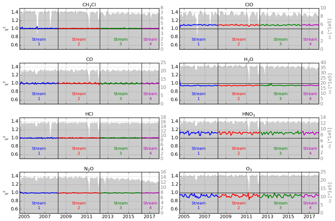
Figure 1Time series of the monthly mean χ2 for MLS assimilated species (coloured lines – one colour for each stream, left y axes) and the corresponding number of assimilated observations m (grey bars, right y axes). The horizontal black lines show the expected theoretical value of χ2=1 and the vertical black lines show the dates of the transition between the different streams.
The system includes two adjustable parameters that need to be calibrated: the model error parameter α and the observational error scaling factor so. The model error is calibrated using a χ2 test. At a given model time step k, measures the difference between the observations and the model forecast weighted by their combined error covariances. Ideally, if the covariances are correctly specified and if the model is un-biased, the average should be close to the number of observations mk, i.e. , where 〈〉 denotes the mathematical expectation. Ménard and Chang (2000) have shown that the slope in the time series of is sensitive to the model error parameter α while the time average of is sensitive to the observational error. For MLS assimilation using BASCOE, Skachko et al. (2014, 2016) found a single value of α=2.5 % for each assimilated species and each model grid point, and the same value was used for BRAM2. For the observational error scaling factor, a vertical profile for each species has been calibrated using the Desroziers’ method (Desroziers et al., 2005) as implemented in Skachko et al. (2016).
Figure 1 shows the time series of the monthly mean for the four streams. The total number of monthly assimilated observations is also shown. For all species, the χ2 time series are stable, as expected. This validates the choice of α=2.5 %. For CH3Cl, CO, HCl and N2O, the values are very close to 1. For ClO and HNO3, the values are slightly higher than 1 (around 1.1), and for H2O and O3, the values are slightly lower than 1 (around 0.95 and 0.9, respectively). The χ2 time series for HNO3 and O3 also display seasonal variations of small amplitude (<0.1). Overall, these deviations are relatively small, e.g. when comparing with a χ2 test obtained by the Tropospheric Chemical Reanalysis (Miyazaki et al., 2015). This validates the implementation of Desroziers’ method to adjust the observational error scaling factors. Note that the transition between the streams does not display visible discontinuities in the χ2 time series, which validates the choice of a 1-month overlap between the streams. (Values for the first month of streams 2–4, which overlap with the last month of streams 1–3, are not shown.)
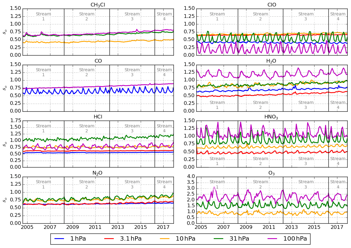
Figure 2Time series of monthly mean observational error scaling factors so for each assimilated species at five specific MLS levels: 1, 3.1, 10, 31 and 100 hPa. The vertical black lines show the dates of the transition between the different streams.
Figure 2 shows the time series of the observational error scaling factors estimated by Desroziers’ method for all species at five selected pressure levels. Values higher (lower) than 1 indicate that the MLS error has been increased (decreased) by the Desroziers’ method. Values are usually between 0.5 and 1.5 except for O3 at 100 hPa, which has a value between 2 and 3, this being likely due to vertical oscillation in MLS O3 profiles in the TTL (see Sect. 5.4). The time series display seasonal variations for some species and/or levels usually with a 6-month period attributed to both polar winter seasons. As for the χ2 test, no discontinuities are visible at the transition time between the streams. For some species and/or levels, the time series show a small positive drift. The cause of this drift has not been identified but is unlikely due to an issue in the BASCOE system. In such a case, this would have resulted in discontinuities at the dates of transition between the streams in the time series of the observational error scaling factors. This issue has not been investigated further in this paper.
3.3 BASCOE observation operator
The observation operator of BASCOE consists of a linear interpolation of the model state to the geolocation of the observed profile points available at the model time ±15 min, i.e. half of the model time step. It has been used to save the BRAM2 state in the space of MLS as well as in the space of the independent observations, except for NDACC ozonesondes, during the BRAM2 production. For NDACC ozonesondes, the BRAM2 state has been interpolated to the NDACC station from the 6-hourly BRAM2 gridded outputs. The error introduced by this method is negligible for O3 below 10 hPa where ozonesondes are used (Geer et al., 2006). Note that no averaging kernels of any satellite dataset have been used in the BASCOE observation operator because the BASCOE EnKF is not ready for their use. The vertical resolution of these observations is sufficiently high – and similar to the model vertical resolution – that their use is typically considered unnecessary. We will see, however, that this is not always the case (see Sect. 5).
3.4 BRAM2 outputs
BRAM2 gridded outputs are the 6-hourly mean of the ensemble state. A second type of output is given in the space of the observations (see previous section) and will be referred to below as model-at-observation or, in short, ModAtObs. All outputs (gridded and ModAtObs) are taken at step 4 of the assimilation cycle (see Sect. 3.1), i.e. corresponding to the background state. For the gridded outputs, this allows the last model forecast to smooth any discontinuities at the edge of regions influenced by observations. For ModAtObs outputs, this means that all comparisons between BRAM2 and observations shown in this paper are using the background state.
3.5 Control run
For this publication, a control run has been produced, labelled CTRL. It is a BASCOE CTM simulation using the same configuration as BRAM2, covering the period May 2009–November 2010, and initialized by the BRAM2 analysis. CTRL is used to evaluate the added value of the assimilation compared to a pure model run where an 18-month simulation is sufficiently long. It will also indicate model processes that need to be improved in the future.
The evaluation of BRAM2 is based on means and standard deviations of the differences between BRAM2 and the assimilated or the independent observations. In all cases, the BRAM2 forecast (or background) is used, i.e. at step 4 of the assimilation cycle (see Sect. 3.1). These statistics are denoted “forecast minus observations” (FmO). FmO are calculated in either pressure–latitude or potential temperature–equivalent latitude domain. In the first case, the statistics are calculated on the MLS pressure grid or, for the other datasets which are given on a kilometric vertical grid, on pressure bins with 12 bins per decade of pressure using the pressure profiles from these datasets. In the second case, all products are interpolated on potential temperature (theta) levels using their measured pressure and temperature profiles. Equivalent latitudes at the observations are interpolated from ERA-Interim daily fields of potential vorticity, at 12:00 UT, calculated on a latitude–longitude grid and with a 35-level theta grid from 320 to 2800 K (Manney et al., 2007). Finally, statistics in percent are normalized to the mean of the BRAM2 forecast corresponding to the same period and region.
The FmO statistics will also be compared to the MLS error budget provided in the MLS data quality document (see L2015). The mean and standard deviations of (BRAM2 − MLS) differences will be compared, respectively, to the MLS accuracy and precision. Depending on the species, these values are provided in volume mixing ratio (vmr), in percent or both. If necessary, the conversion from percent to vmr, and vice versa, will use MLS average observations corresponding to the shown situation.
In order to determine if the origin of the biases between BRAM2 and independent observations is due to MLS or the BASCOE CTM, the FmO statistics have also been compared to the mean and standard deviation of the difference between MLS and ACE-FTS as provided in other validation studies. These values have been digitized from Froidevaux et al. (2008b) for HCl, Santee et al. (2013) for CH3Cl, and Sheese et al. (2017, denoted hereafter S2017) for O3, H2O, N2O, HNO3 and CO (for CO, only during polar winter conditions). Error profiles from S2017 are converted from a kilometric to a pressure vertical grid using a log-pressure–altitude relationship with a scale height of 7 km. Santee et al. (2013) and S2017 also show the mean profiles of MLS and ACE-FTS used to make their comparison, allowing us to convert from percent to vmr. For Froidevaux et al. (2008b), this conversion is based on the average MLS observations corresponding to the shown situation.
Figure 3 displays the daily zonal means of MLS, BRAM2 and CTRL on 1 September 2009 for O3, H2O, N2O, HNO3, HCl, ClO (daytime values), CH3Cl and CO. Only BRAM2 species constrained by MLS will be evaluated in this paper. This figure highlights regions of good and poor qualitative agreement between BRAM2 and MLS and the added value of the assimilation compared to a pure model run (CTRL). The figure also highlights regions with chemical or dynamical regimes that will be explored in more detail in this section.
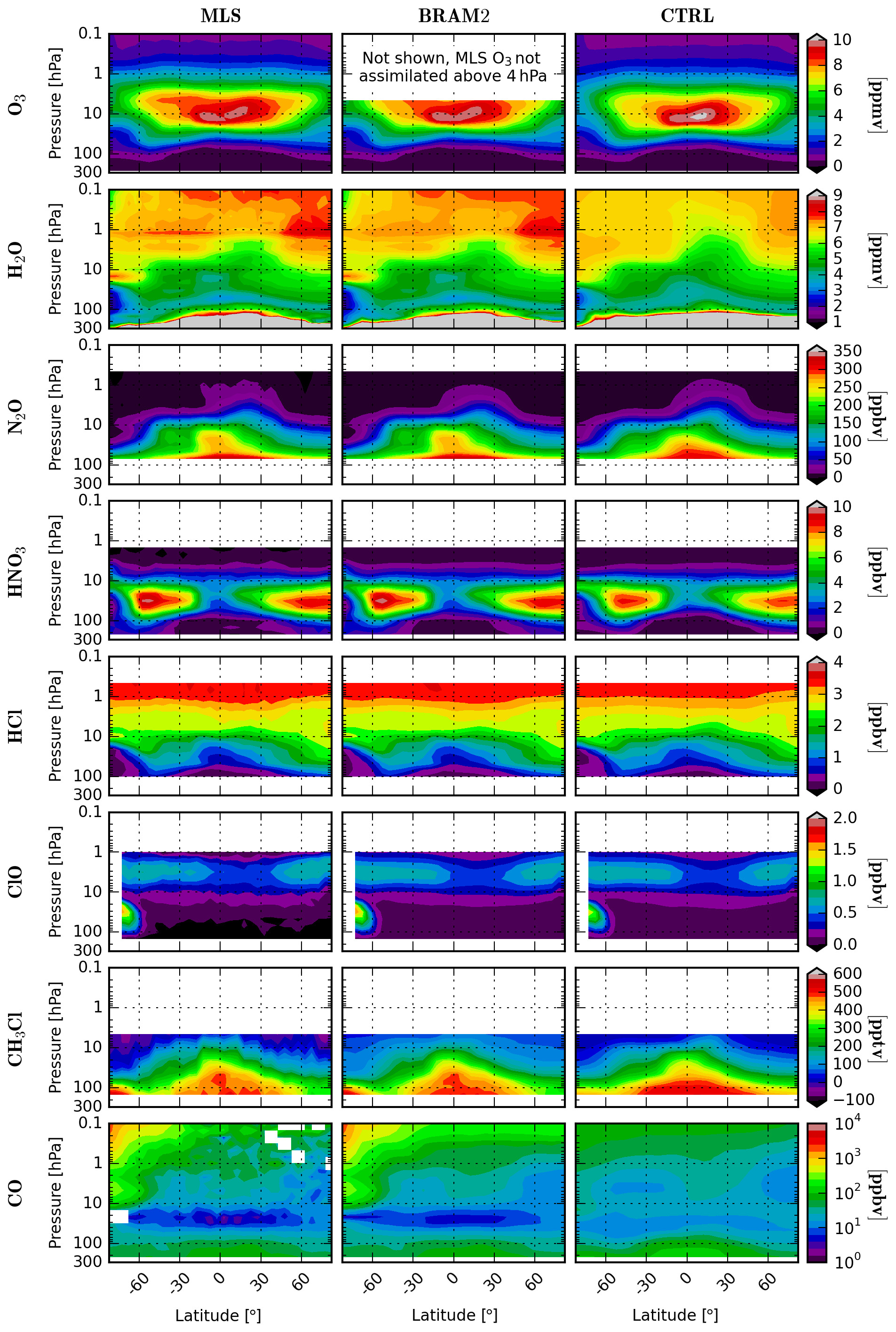
Figure 3Daily zonal means of MLS observations (left column) on 1 September 2009, the corresponding ModAtObs values of BRAM2 (centre column) and CTRL (right column). From top to bottom: O3 (ppmv), H2O (ppmv), N2O (ppbv), HNO3 (ppbv), HCl (ppbv), ClO (ppbv, daytime values), CH3Cl (pptv) and CO (ppbv, note the log scale). Zonal means are calculated on the MLS pressure grid and binned on a 5∘ latitude grid. White squares in the MLS CO plot denote negative values. BRAM2 O3 is not assimilated (and not shown) at an altitude above 4 hPa; see text for details.
One of these regions is the lower stratosphere in the polar vortex (denoted hereafter LSPV) where PSC microphysics take place. In this region (between 10 and 100 hPa and between 90 and 60∘ S in the figure), HNO3 and H2O are lost due to PSC uptake and sedimentation, HCl is destroyed by heterogeneous chemistry on the surface of PSCs, and ClO is produced. All these features, observed by MLS, are reproduced well by BRAM2. The comparison of BRAM2 and CTRL highlights some model deficiencies, e.g. the underestimation of H2O loss and ClO enhancement. The isolation of polar air from mid-latitudes is also visible by the strong N2O horizontal gradient around 60∘ S, observed by MLS, reproduced well by BRAM2 and underestimated in CTRL. Another region is the upper stratosphere–lower mesosphere (USLM) in the polar vortex (hereafter denoted USPV). This region (between 0.1 and 10 hPa and between 90 and 60∘ S in the figure) is affected by the descent of mesospheric and thermospheric air rich in CO and poor in H2O. BASCOE does not include upper boundary conditions for these sources and losses so CTRL displays much higher H2O and much lower CO than MLS in USPV. BRAM2 on the other hand agrees well with the observations.
The third identified region is the UTLS, where, in the tropics (between 70 and 300 hPa), tropospheric source gases enter in the stratosphere. Relevant species in this region are H2O, O3, CH3Cl and CO (N2O would have been relevant but the MLS N2O retrieval is not recommended for scientific use at pressures greater than – altitudes below – 68 hPa). BRAM2 agrees well with MLS in this region for these species. It improves the vertical gradient of H2O found in CTRL and the amount of CO and CH3Cl.
The fourth region includes everything not in the LSPV, USPV and UTLS regions. Since it covers most of the middle stratosphere, it will be denoted MS. In this region, BRAM2 and MLS agree generally well, e.g. at the ozone peak, for the horizontal gradient of N2O and the vertical gradient of HCl.
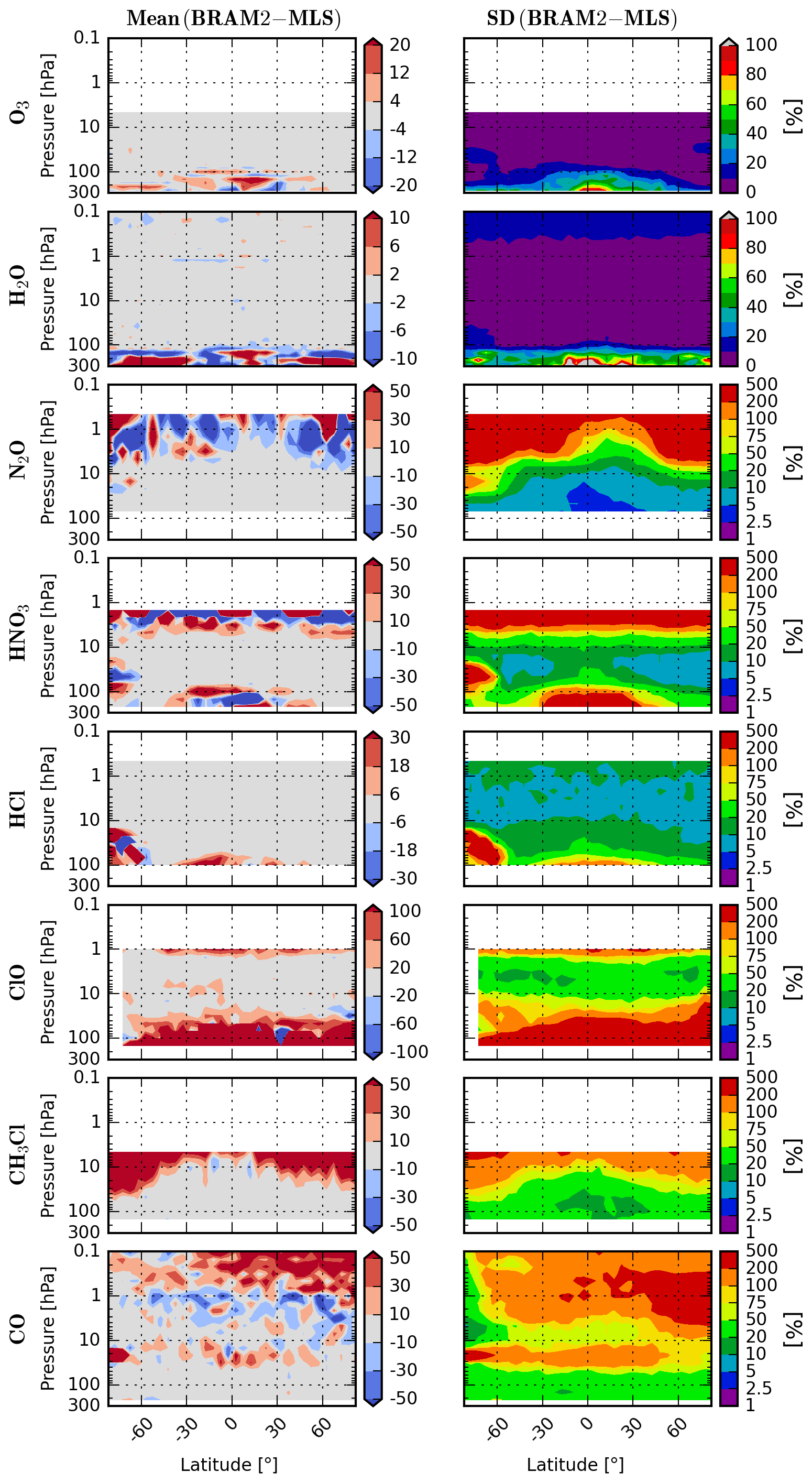
Figure 4Daily zonal mean differences (%) between BRAM2 and MLS (left column) and the associated standard deviation (right column) on 1 September 2009. From top to bottom: O3, H2O, N2O, HNO3, HCl, daytime ClO, CH3Cl and CO. Zonal means are calculated on the MLS pressure grid and binned on a 5∘ latitude grid. Note that the ranges in the colour bars differ for each individual plot and that some colour bars are on a log scale.
Figure 4 shows the mean and standard deviation of the differences between BRAM2 and MLS, associated with their daily zonal mean shown in Fig. 3. These statistics are in percent and are normalized by the mean of BRAM2, as will be the case for the rest of the paper. In general, the normalized mean and standard deviation of the differences are low where the abundance of the species is relatively high, with the exception of H2O in the upper troposphere. Conversely, the (normalized) mean and standard deviation are high where the abundance of the species is low, i.e. (1) O3 in the tropical troposphere; (2) N2O above 5 hPa and in the polar vortex; (3) HNO3 in the UTLS, above 5 hPa and in the polar vortex; (4) HCl in the UTLS and in the polar vortex, (5) ClO in the lower stratosphere, (6) CH3Cl above 10 and 30 hPa in, respectively, the tropics and the mid-latitudes; and (7) CO in the MS and LSPV.
In the following subsections, BRAM2 will be evaluated in the four above-mentioned regions: the middle stratosphere (MS), the lower-stratospheric polar vortex (LSPV), the upper-stratospheric–lower-mesospheric polar vortex (USPV) and the upper troposphere–lower stratosphere (UTLS). The objective of these evaluations is to answer several questions. How well does BRAM2 agree with assimilated and independent observations? In which regions and altitudes is BRAM2 recommended for scientific use, i.e. well characterized against independent observations with FmO statistics stable in time? For this evaluation, we have used five well-characterized sets of independent observations: ACE-FTS, MIPAS, SMILES ClO, MLS_N2O_640 (the other MLS N2O product retrieved from the 640 GHz radiometer which was turned off in July 2013) and ozonesondes. A summary of the evaluation is given in Sect. 5.5 and a note on the BRAM2 unobserved species is given in Sect. 5.6.
5.1 Middle stratosphere (MS)
The evaluation of BRAM2 in the middle stratosphere is based on two figures and one table: one figure showing vertical profiles of the FmO (Fig. 5), the other showing time series of the FmO at selected pressure levels (Fig. 6) and the table providing the FmO statistics at three pressure levels (Table 1). The first figure shows the mean and standard deviation of the FmO between BRAM2 and observations from MLS, ACE-FTS, MIPAS, MLS_N2O_640, SMILES ClO and ozonesondes. These statistics are calculated between 30 and 60∘ N and between 0.1 and 100 hPa for the 2005–2017 period for MLS and ACE-FTS (FmO profiles between 60 and 30∘ S and between 30∘ S and 30∘ N are given in the Supplement). For MIPAS and MLS_N2O_640, the datasets end in March 2012 and July 2013, respectively. For SMILES, the period is October 2009–April 2010. Note that comparison with MIPAS ClO is only performed in the polar winter conditions (see Sect. 2.2.2). CO is not shown in the figure because it is chemically irrelevant in the middle stratosphere – CO will be discussed in the USPV and the UTLS subsections. The figure also shows two types of error: first, the MLS accuracy and precision which are compared, respectively, to the mean and the standard deviation of the differences, and, second, the mean and standard deviation of the differences between MLS and ACE-FTS (see Sect. 4).
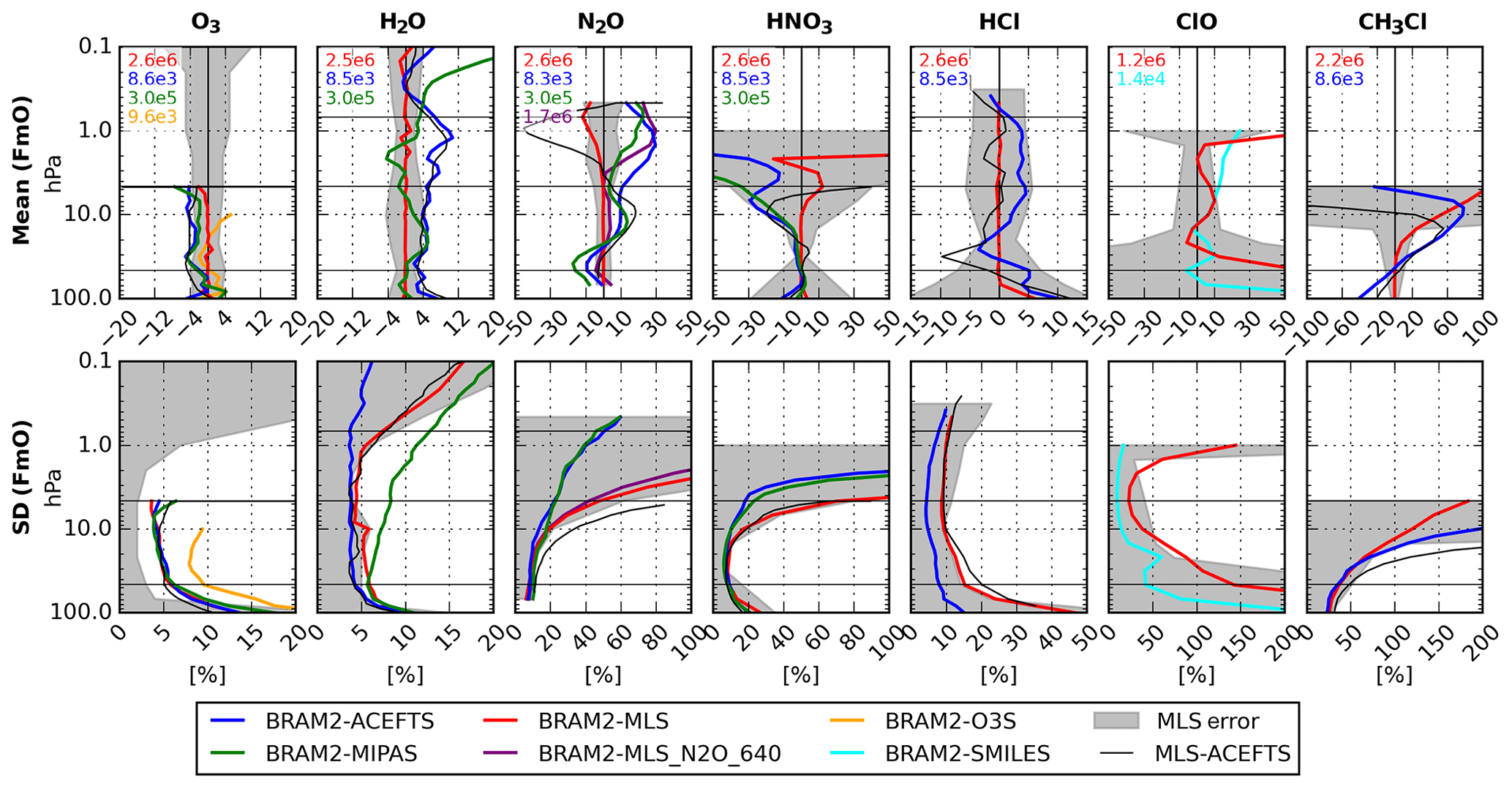
Figure 5Mean (top row) and standard deviation (bottom row) of the differences between BRAM2 and observations from MLS (red lines), ACE-FTS (blue lines), MIPAS (green lines), MLS_N2O_640 (purple lines), NDACC ozonesondes (orange lines) and SMILES (cyan lines). The statistics are in percent, normalized by the mean of BRAM2, and are taken between 30 and 60∘ N and between 0.1 and 100 hPa. The period is 2005–2017 except for MIPAS (2005–2012), MLS_N2O_640 (2005–2013) and SMILES (October 2009–April 2010). The statistics are calculated for, from left to right, O3, H2O, N2O, HNO3, HCl, daytime ClO and CH3Cl. The approximate numbers of observed profiles used in the FmO statistics are given in the upper left corner of the top row plots using the instrument colour code. The grey shaded area in the mean and standard deviation plots corresponds, respectively, to the MLS accuracy and precision, as provided in the MLS data quality document (see L2015). The thin black profiles represent the mean (top row) and standard deviations (bottom row) between MLS and ACE-FTS found in validation publications (see text for details). The horizontal black lines denote levels where time series are shown in Fig. 6.
The second figure (Fig. 6) shows time series of monthly FmO for the 2005–2017 period corresponding to the 30–60∘ N latitude band at three pressure levels in the high, middle and lower stratosphere: 0.68, 4.6 and 46 hPa. Statistics shown are the bias against the different instruments and the standard deviation against ACE-FTS (FmO time series between 60 and 30∘ S and between 30∘ S and 30∘ N are given in the Supplement). For ClO, which is not retrieved in ACE-FTS v3.6, the standard deviation against SMILES is shown. The time series are in percent except for ClO, which is in parts per billion by volume. For this species, only daytime observations are taken into account in Figs. 5 and 6.
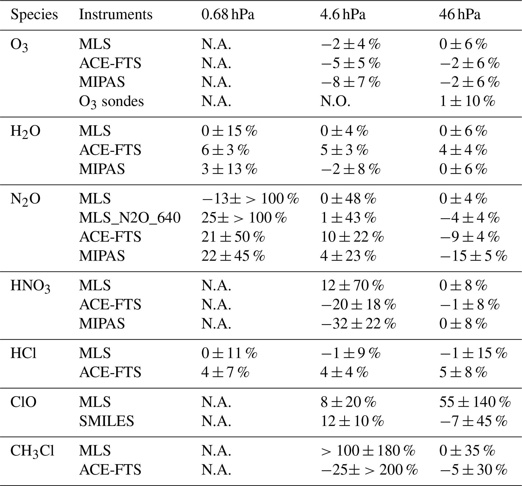
In general, BRAM2 represents a good proxy for MLS. The biases against MLS are smaller than the MLS accuracy so that they are not significant (Fig. 5). Moreover, the standard deviations against MLS and the MLS precision are usually in good agreement, except for O3. Time series of the bias against MLS is in general very stable with negligible amplitude in the seasonal variations, except for N2O at 0.68 hPa, HNO3 at 4.6 hPa, ClO at 4.6, and 46 hPa and CH3Cl at 4.6 hPa (see Fig. 6).
The standard deviation against ACE-FTS is usually smaller than the standard deviation against MLS, which indicates that the variability in MLS observations is larger than that in ACE-FTS (Fig. 5). Also, the standard deviation against ACE-FTS is usually stable in time (Fig. 6).
The biases against ACE-FTS are in general similar to the differences between MLS and ACE-FTS calculated in published validation studies (see Sect. 4), except for HCl, N2O above 3 hPa, HNO3 above 10 hPa and CH3Cl above 20 hPa. This means that most of the differences between BRAM2 and the independent observations are due to the difference between these datasets and MLS. Also, the standard deviations against ACE-FTS are as good as or better than those from direct comparisons between MLS and ACE-FTS (except for O3 below 40 hPa). This suggests that a significant part of the standard deviations of (MLS − ACE-FTS) calculated in validation studies are due to sampling error introduced by the collocation approach. In our case, the sampling error is replaced by the representativeness error arising from the limited spatial and temporal resolution of the data assimilation system. We thus conclude that the representativeness errors within BRAM2 are smaller than the sampling errors inherent in validation studies based on collocation of profiles.
Thus, in general, BRAM2 mean values and their variability agree well with the observations. Let us now discuss these statistics from species to species (see Sect. 5.5 for a summary of BRAM2 evaluation in the different regions). This discussion is mainly qualitative and the reader should refer to Table 1 for quantitative results.
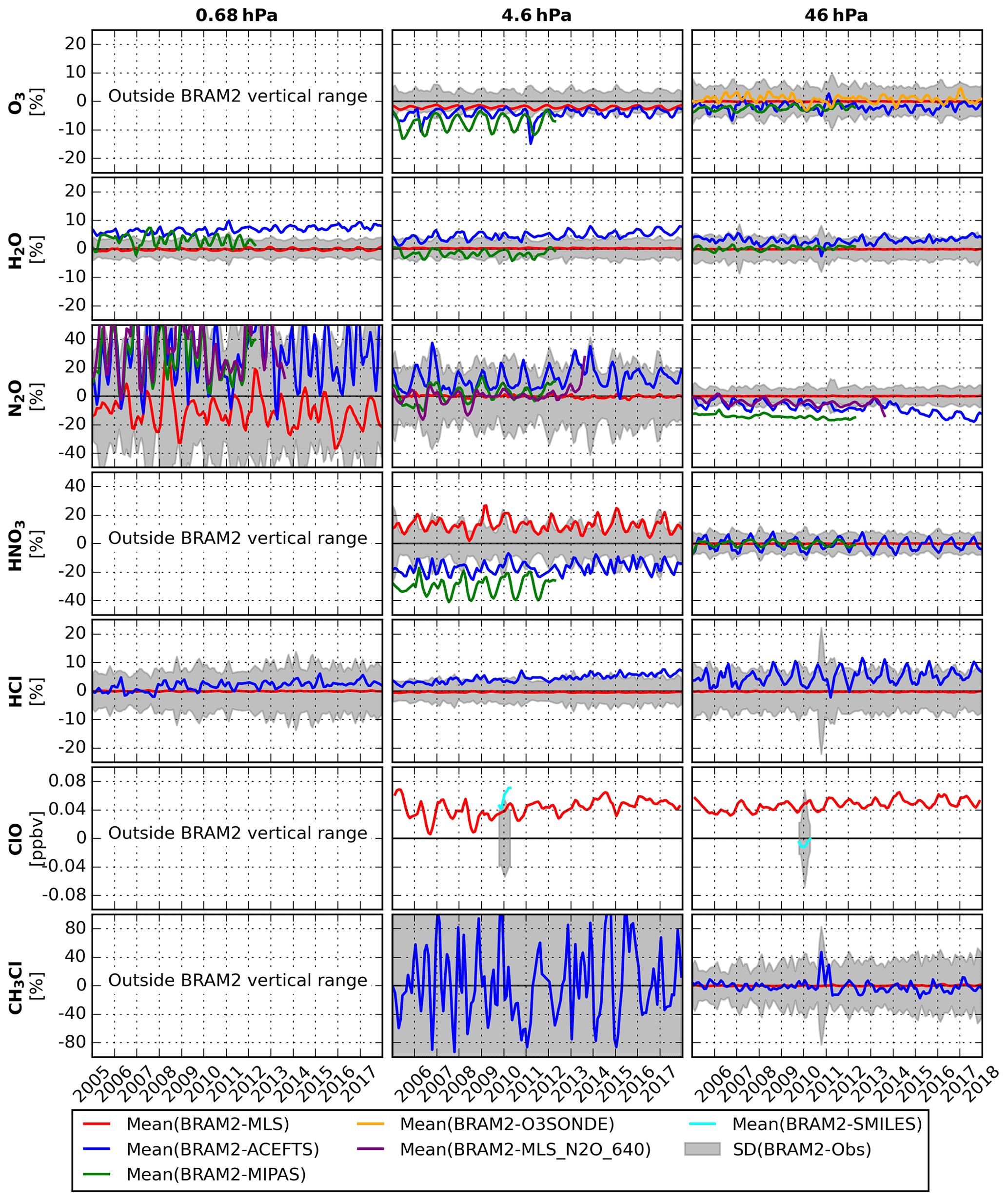
Figure 6Time series of the monthly mean differences between BRAM2 and the different observational datasets in the Northern Hemisphere mid-latitudes (30–60∘ N) at three pressure levels (from left to right: 0.68, 4.6 and 46 hPa) and for (top to bottom) O3, H2O, N2O, HNO3, HCl, daytime ClO and CH3Cl. Values are in percent except for ClO, which is shown in parts per billion by volume. The grey shaded area represents the standard deviation of the differences between BRAM2 and ACE-FTS except for ClO, where SMILES data are used.
Table 1Mean difference and standard deviation between BRAM2 and observations for the 2005–2017 period at three specific levels in the middle stratosphere: 0.68, 4.6 and 46 hPa. Values are in percent, normalized by BRAM2. Abbreviations: not assimilated (N.A.) and not observed (N.O.).
O3. We recall that ozone is not assimilated at altitudes higher (i.e. pressure lower) than 4 hPa due to a BASCOE model ozone deficit (see Sect. 3.1), and comparisons above that level are not shown. Below that level, BRAM2 agrees well with all instruments (see Fig. 5 and Table 1). The bias against MLS is almost negligible and is negative against ACE-FTS and MIPAS. The standard deviation profiles against MLS, ACE-FTS and MIPAS are similar, and the standard deviation against ozonesondes is usually larger by around 5 %, likely due to the higher representativeness of ozonesondes against the model.
Time series of the bias against all instruments at 4.6 and 46 hPa are stable from year to year, with small seasonal variations (substantially higher against MIPAS at 4.6 hPa; see Fig. 6). The standard deviations against ACE-FTS are small with small seasonal variations at 4.6 and 46 hPa. Similar statistics are found in the southern hemispheric mid-latitudes and in the tropics above 50 hPa (see Figs. S1–S4 in the Supplement). Given the good agreement between BRAM2 and the observations, we recommend BRAM2 O3 in the MS for scientific use between 4 and 100 hPa.
H2O. The general agreement with MLS, ACE-FTS and MIPAS is very good below 1 hPa (see Fig. 5 and Table 1). Above that level, the bias against MIPAS increases, as well as the standard deviation against MLS and MIPAS, although to a reasonable extent in all cases. Bias against ACE-FTS is positive below 0.5 hPa.
Biases are stable over time, with small seasonal variation between 0.68 and 46 hPa (Fig. 6). Standard deviations against ACE-FTS are also stable, displaying negligible seasonal variations. As for ozone, similar statistics are found in the Southern Hemisphere and in the tropics above 50 hPa (see Figs. S1–S4), and we recommend BRAM2 H2O for scientific use in these regions.
N2O. At altitudes below 10 hPa, BRAM2 agrees well with MLS and independent observations from MLS_N2O_640, ACE-FTS and MIPAS (Fig. 5 and Table 1). From 10 hPa to higher altitudes (i.e. lower pressure), the standard deviations increase with larger values against MLS and MLS_N2O_640 than against ACE-FTS and MIPAS.
Above 3 hPa, BRAM2 is poorly characterized by comparison against observations. The standard deviations against MLS are large (Fig. 5), and the time series of the FmO are noisy, with large peak-to-peak variations. In the upper stratosphere, the MLS precision degrades to around 65 % at 2 hPa, which limits the constraint of the assimilated observations on the reanalysis.
Bias between BRAM2 and MLS is stable (and small) over time at 4.6 hPa (Fig. 6), which is not the case for the bias between BRAM2 and the independent observations. At 46 hPa, the bias with independent observations is small but increases over the time, suggesting a positive drift in BRAM2. Analyses of the deseasonalized time series of the biases reveal a significant drift of −5, −7 and −5 % per decade against ACE-FTS, MIPAS and MLS_N2O_640 for the period 2005–2012 and −10 % against ACE-FTS for 2005–2017 (not shown). This drift has been mentioned in Froidevaux et al. (2019) and is under investigation by the MLS team (Livesey et al., 2019).
Similar agreement is found in other latitude regions (see Figs. S1–S4). Therefore at altitudes below 3 hPa and excluding trend analysis, we recommend BRAM2 N2O for scientific use in the middle stratosphere. At altitudes above 3 hPa, BRAM2 should not be used without consulting the BASCOE team.
HNO3. At altitudes below 10 hPa, BRAM2 agrees well with MLS, ACE-FTS and MIPAS (see Fig. 5 and Table 1). From 10 to 3 hPa, the bias against ACE-FTS and MIPAS increases to relatively large values (with a negative sign), as well as the standard deviation against MLS. On the other hand, the standard deviations against ACE-FTS and MIPAS remain relatively small. Above 3 hPa, BRAM2 HNO3 is poorly characterized by comparison against observations. The biases against the three instruments are large and disagree in sign and size (Fig. 5). Above that level, MLS precision degrades (reaching 0.6 ppbv, i.e. 6 times the typical amount of HNO3 at that level), and the constraint by the assimilated observations on BASCOE is weak.
These values are stable over the years at 4.6 and 46 hPa, while displaying significant seasonal oscillations at 4.6 hPa (Fig. 6). These seasonal variations may be due to including observations belonging to the polar vortex or the tropical region, the 30–60∘ N region not being a strict definition of the mid-latitudes of the Northern Hemisphere. At 4.6 hPa, the standard deviation against ACE-FTS displays significant seasonal oscillation, from ∼10 % during summer to ∼20 % during winter, likely due to the polar influence during the winter.
Similar statistics are found in the Southern Hemisphere and in the tropics (see Figs. S1–S4), and we recommend BRAM2 HNO3 for scientific use between 3 and 100 hPa. The use of BRAM2 HNO3 above 3 hPa should be carried out in consultation with the BASCOE team.
HCl. BRAM2 agrees well with MIPAS and ACE-FTS between 0.4 and 70 hPa (see Fig. 5 and Table 1, this pressure range being reduced to 0.4–50 hPa in the tropics; see Fig. S2). At 100 hPa, the bias increases (positive values) with larger values in the tropics than at mid-latitudes. The difference (BRAM2 − ACE-FTS) is larger by around 5 % than the difference (MLS − ACE-FTS) from Froidevaux et al. (2008b). This is due to the different versions of MLS and ACE-FTS used here (v4 and v3.6, respectively) and in Froidevaux et al. (2008b, using v2 and v2.2) and the fact that the HCl amount has been reduced by around 5 % in the latest version of ACE-FTS data (Waymark et al., 2013). Our comparison is thus an update of Froidevaux et al. (2008b). Also note the lower standard deviation against ACE-FTS than against MLS, suggesting higher precision of ACE-FTS compared to MLS.
Bias time series are very stable against MLS with negligible seasonal variations (Fig. 6). On the other hand, a small drift is noticeable in the bias time series against ACE-FTS at 0.68 and 4.6 hPa. The MLS HCl v4 standard product assimilated for BRAM2 is retrieved from band 14 of the 640 GHz radiometer, while band 13 – more sensitive to HCl – was originally planned. This change of strategy by the MLS retrieval team was due to the deterioration of band 13, which was turned off in 2006 (see L2015). For this reason, the MLS HCl values from band 14 (and BRAM2) are not suited for detailed trend studies in the USLM.
Based on these comparisons, we recommend BRAM2 HCl for scientific use between 0.4 and 100 hPa (50 hPa in the tropics), but it cannot be used for trend studies.
ClO. For ClO, the analysis increments are very small in the middle stratosphere and the bias (BRAM2 − MLS) and (CTRL − MLS) are similar, as suggested by Fig. 3. There is a relatively good agreement with MLS and SMILES between 1.5 and 30 hPa (see Fig. 5 and Table 1). Note the lower standard deviations against SMILES in this altitude range, suggesting higher precision of SMILES compared to MLS. Comparison against MIPAS ClO is not shown because MIPAS V5_ClO_22[0_or_1] is only valid under conditions of chlorine activation in the polar winter (see Sect. 2.2.2).
Time series of the bias against MLS show small seasonal variations at 4.6 and 46 hPa (Fig. 6). Similar values are found in the southern mid-latitudes and in the tropics (see Figs. S1–S4). We conclude that BRAM2 ClO in the middle stratosphere is more a CTM product than a data assimilation product. Nevertheless, BRAM2 ClO in the middle stratosphere can be recommended for scientific use between 1 and 70 hPa and should be used in consultation with the BASCOE team outside this vertical range.
CH3Cl. Below 30 hPa, BRAM2 agrees relatively well with MLS (see Fig. 5 and Table 1). The FmO values are usually larger than for other species due to the higher MLS uncertainties for this species. The bias against ACE-FTS is larger, being negative at 100 hPa to positive at 10 hPa. The standard deviations against both instruments are similar below 30 hPa. At 46 hPa, the time series of the biases display negligible seasonal variations against MLS and small seasonal variations against ACE-FTS (see Fig. 6). (Spikes in the ACE-FTS time series around 2010/2011 are due to (1) the small number of ACE-FTS profiles in October 2010 and February 2011 and (2) the fact that some of them display unphysical vertical oscillations – not shown.) The agreement with MLS and ACE-FTS is better in the tropics (see Figs. S2 and S4).
Above 30 hPa at mid-latitudes (10 hPa in the tropics), the agreement between BRAM2 and MLS degrades. More worrying is that CTRL agrees better with MLS observations than BRAM2 (see Fig. 3), indicating that MLS observations are not properly assimilated. The reason for this issue is probably twofold. First, there is a relatively large number of negative MLS CH3Cl observations above 10 hPa, and, second, the MLS averaging kernels are not used in the BASCOE observation operator. Assimilating negative data is not an issue as long as the overall analysis is positive, which is not always the case with CH3Cl. In BASCOE, negative analyses are clipped to nearly zero (10−25), which in the case of CH3Cl introduces a positive bias in the analysis. Since significant information in the retrieved profiles comes from the a priori profiles above 10 hPa (see L2015, their Fig. 3.3.2), the use of the averaging kernels would help to ensure positiveness of the analysis. Unfortunately, this issue was not considered before starting the production of BRAM2. Consequently, we recommend the use of BRAM2 CH3Cl only below 30 hPa at mid-latitudes and 10 hPa in the tropics.
5.2 Lower-stratospheric polar vortex (LSPV)
Figure 7 shows the evolution of the southern hemispheric (SH) polar vortex composition from MLS observations, BRAM2 and CTRL in 2009. Values correspond to daily means in the inner vortex, i.e. between 90 and 75∘ S of equivalent latitude. The vertical domain is between 320 and 700 K potential temperature, approximately between 100 and 10 hPa. The SH inner polar vortex was chosen because it is the region where CTRL differs most from the reanalysis. Evaluating BRAM2 in these conditions is thus a stronger test for the quality of the reanalysis. The species shown in Fig. 7 and discussed throughout this section are O3, H2O, N2O, HNO3, HCl and ClO. For ClO, only daytime values are taken into account.
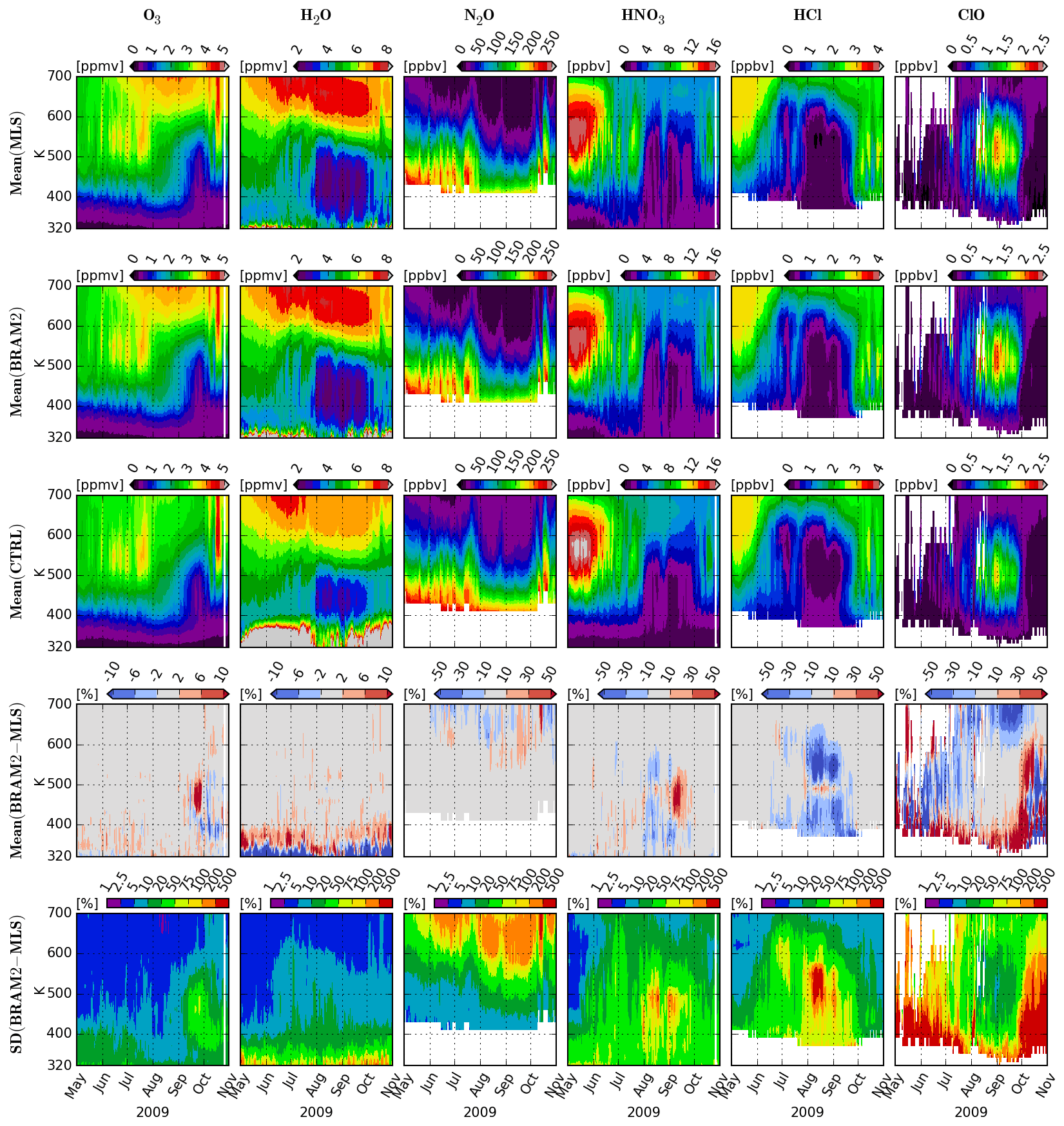
Figure 7Time series of (from top to bottom) daily mean MLS profiles, the corresponding values of BRAM2, the corresponding values of CTRL, the relative mean difference (%) between BRAM2 and MLS and the associated standard deviation (%). Values are shown between May and November 2009 in the lower-stratospheric inner vortex (i.e. within 90–75∘ S equivalent latitude and within 320–700 K) for (from left to right) O3, H2O, N2O, HNO3, HCl and ClO. Only daytime values of ClO are considered in the mean calculations. White areas correspond to locations and dates without valid observations.
Qualitatively, there is a very good agreement between BRAM2 and MLS, as expected, for the patterns associated with both chemical and dynamical processes. For the chemistry, the loss of HCl by heterogeneous chemistry and the activation of ClO are reproduced well by BRAM2, as is the loss of HNO3 and H2O by denitrification and dehydration. The ozone depletion in BRAM2 that occurs in September–October is also in very good agreement with MLS. Dynamical patterns are also in good agreement. The descent of air from above 700 K that starts in May and ends in October, exhibited by the decrease in N2O and the increase in H2O and O3, is reproduced well by BRAM2. Dynamical patterns of shorter timescales are also reproduced well by BRAM2, e.g. the increase in N2O in late July and late August.
Comparison between the CTRL and BRAM2 shows the regions where MLS observations correct the bias in the BASCOE CTM. For chemical patterns, the loss of HCl is relatively well represented in the model, between 450 and 650 K. Below 450 K, modelled HCl overestimates the observations. Above 400 K, the loss of HNO3 is also reproduced well by the model while the model has a negative bias below that level. The model also slightly underestimates the ClO activation and the loss of H2O by dehydration. The good performance of CTRL, especially for HCl, contrasts with recent studies showing the difficulties of CTMs (Lagrangian and Eulerian) to simulate the loss of HCl by heterogeneous chemistry (Wohltmann et al., 2017; Grooß et al., 2018). Note that the BASCOE CTM is based on a relatively simple PSC parameterization and that its parameters have been tuned to improve the model representation (see Sect. 3.1). In other words, it does not include the state of the art of heterogeneous chemistry treatment as in these other studies, and this setup is justified to create a reanalysis in good agreement with observations.
For dynamical patterns, CTRL shows a more pronounced bias. Descent of air (exhibited by high values of H2O and low values of N2O between 600 and 700 K), which is correctly reproduced from the beginning of the simulation, is abruptly interrupted in July, probably due to a weakening of the polar vortex at that time. This bias can be attributed to the coarse horizontal resolution of the model (Strahan and Polansky, 2006) and is successfully corrected in BRAM2.
Figure 7 also displays the daily mean and standard deviation of the differences between BRAM2 and MLS. The differences are normalized by the daily mean of BRAM2. The differences between CTRL and MLS are shown in Fig. S5. In general, large biases (around 50 %) correspond to conditions with very low absolute values, i.e. for (1) HNO3 and HCl between July and October and below 650 K, (2) ClO outside conditions of chlorine activation, and (3) N2O between 600 and 700 K during the descent of upper-stratospheric air. Large bias also occurs for H2O below 400 K, i.e. in the UTLS. When chlorine is activated (i.e. when ClO abundance is greater than 1 ppbv), the mean differences between BRAM2 and MLS are below 10 %, well within the MLS accuracy (0.1 ppbv; see L2015). Bias also increases for O3 in late September, during the development of the ozone hole, but to a reasonable magnitude (10 %).
The standard deviations of the differences also increase when the concentration of the species is very low. In particular, the standard deviation can be higher than 100 % for N2O between 600 and 700 K during the descent of upper-stratospheric air and for HNO3 and HCl between July and October and below 650 K. In these cases, standard deviations are more relevant when unnormalized (i.e. in vmr units) and the corresponding values for these three species are, respectively, 10, 0.2 and 0.1 ppbv (not shown). The standard deviation for O3 also increases and is at a maximum (between 25 % and 50 %) in late September between 400 and 500 K.
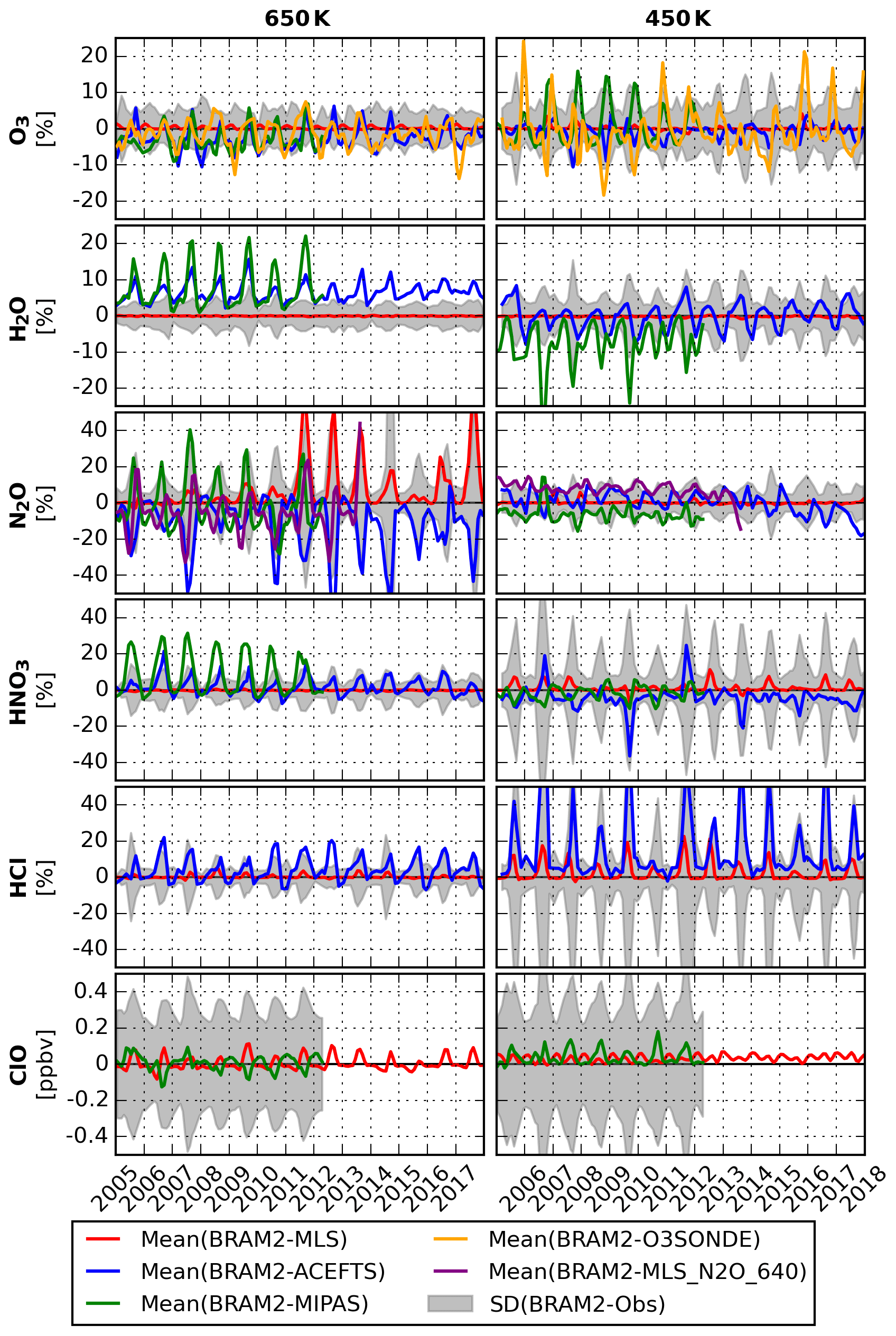
Figure 8Time series of the monthly mean differences between BRAM2 and the different observational datasets between 90 and 75∘ S of equivalent latitude at two potential temperature levels (from left to right: 650 and 450 K) and for (top to bottom) O3, H2O, N2O, HNO3, HCl and daytime ClO. Values are in percent except for ClO, which is shown in parts per billion by volume. The grey shaded area represents the standard deviation of the differences between BRAM2 and ACE-FTS except for ClO where MIPAS data are used.
Table 2Mean difference and standard deviation between BRAM2 and observations in the Antarctic inner vortex (between 90 and 75∘ of equivalent latitude) at 650 and 450 K of potential temperature and between June and November of the 2005–2017 period. Values in percent are relative to BRAM2. Abbreviations: not assimilated (N.A.) and not observed (N.O.).
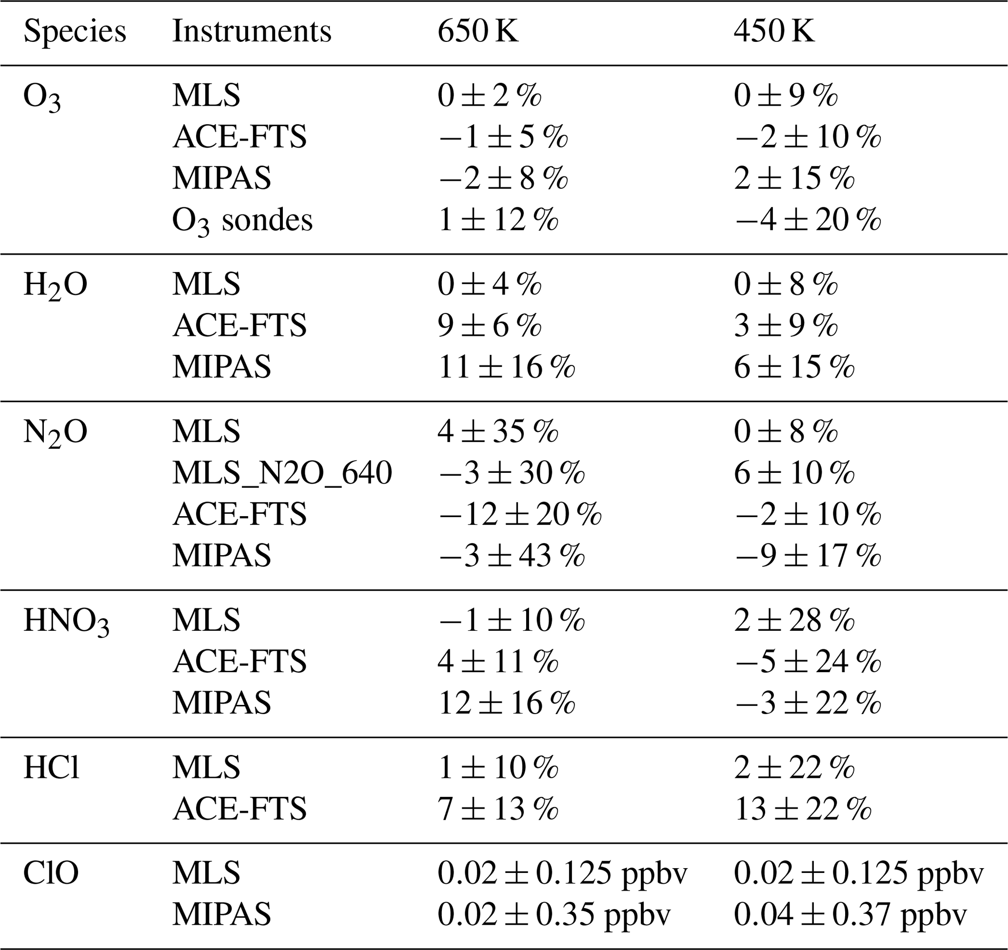
Comparison of BRAM2 in LSPV conditions with independent observations and for years other than 2009 is shown in Fig. 8 and summarized in Table 2. It shows time series of monthly FmO between 90 and 75∘ S of equivalent latitude for the 2005–2017 period and at two potential temperature levels: 650 and 450 K (∼15 and ∼50 hPa, similar figures for the outer vortex and the Arctic winters are shown in the Supplement). Statistics shown are the bias against the different instruments and the standard deviation against ACE-FTS. For ClO, which is not retrieved in ACE-FTS v3.6, the standard deviation against MIPAS is shown. The time series are in percent except for ClO, which is shown in parts per billion by volume. For this species, only daytime observations are taken into account. As expected, comparisons against MLS provide lower biases than against independent observations. Let us discuss Fig. 8 for each species individually.
O3. BRAM2 agrees well with MLS, ACE-FTS and MIPAS. Although also in good agreement, larger differences occur against ozonesondes, likely due to their higher representativeness. Compared to intercomparison between instrument climatologies, performed in SPARC (2017, Figs. 4.1.19 and 4.1.20), the comparison of BRAM2 against independent data displays lower biases. The standard deviations against ACE-FTS are generally smaller than 10 % with larger values (around 15 %) in the lower stratosphere (450 K) during Antarctic springs. We recommend the use of BRAM2 O3 for scientific use in the LSPV.
H2O. BRAM2 agrees well with MLS and ACE-FTS although displaying larger seasonal variations against the latter. The biases against MIPAS are larger with larger seasonal variations, in particular at 650 K where the descent of upper-atmospheric air is significant. In cold conditions (i.e. during polar winter at 650 K), the MIPAS averaging kernels (AKs) are smoother than in warm conditions (i.e. during polar summer). These AKs were applied to a few BRAM2 ModAtObs profiles at MIPAS during summer and winter polar conditions, resulting in a better agreement with MIPAS (not shown). We recommend the use of BRAM2 H2O for scientific use in the lower-stratospheric polar vortex.
N2O. The amount of N2O decreases during polar winter, in particular at 650 K in the beginning of Antarctic spring. While the normalized differences against MLS and the independent observations can be greater than 50 %, the unnormalized differences are always <20 ppbv and typically <10 ppbv, which is small (see typical values in Fig. 7). At 650 K, the standard deviation against ACE-FTS displays larger seasonal variations (up to 20 %–50 % in early spring). At 450 K, where the abundance of N2O is larger, the agreement between BRAM2 and the observations is better. As discussed in Sect. 5.1, one can see a drift between BRAM2 and the independent datasets, likely due to a drift in the MLS N2O standard product. Overall, BRAM2 N2O is reliable in the LSPV and is recommended for scientific use except for trend studies.
HNO3. At 650 K, BRAM2 agrees very well with MLS and has a relatively small positive bias against ACE-FTS and MIPAS. This bias is of opposite sign compared to those in the middle stratosphere, in agreement with observation intercomparison (SPARC, 2017, their Fig. 4.13.3). At 450 K, where HNO3 is lost by PSC uptake and denitrification, the agreement of BRAM2 with those instruments is slightly less good. For example, BRAM2 overestimates MLS during late winter–early spring by around 5 %, which is, nevertheless, within the MLS accuracy. The standard deviation of the differences against ACE-FTS is larger during the denitrification period (reaching 20 % to 50 % depending on the year). This means that data assimilation can correct the model bias due to the BASCOE PSC parameterization but does little to improve its lack of precision. Overall, BRAM2 HNO3 in LSPV is a reliable product and is recommended for scientific use even though it is affected by a large positive relative bias (but small when unnormalized) in regions completely denitrified by PSC sedimentation.
HCl. Similar conclusions hold for HCl. BRAM2 agrees relatively well with MLS and ACE-FTS at 650 K, at the upper limit of PSC activity (see Fig. 7). At 450 K, larger relative differences occur, where BRAM2 usually overestimates the observations, even though the unnormalized differences remain small (e.g. 0.2±0.2 ppbv against ACE-FTS, not shown). Again, as for HNO3, BRAM2 HCl in the LSPV is a reliable product and is recommended for scientific use even though it is affected by large positive relative bias (but small when unnormalized) in regions where HCl has been completely destroyed by heterogeneous reactions on the surface of PSCs.
ClO. Because the abundance of ClO can change by 1 to 2 orders of magnitude from “quiet” periods to periods of chlorine activation, FmO values for ClO are shown in parts per billion by volume in Fig. 8 and Table 2. In general, the agreement with MLS and MIPAS is relatively good during the period of activation. For example, the bias is between 0.02 and 0.04 ppbv, which is small compared to a total abundance between 0.5 and 2.5 ppbv (see Fig. 7). Comparison of BRAM2 with SMILES ClO has been carried out for the chlorine activation period in the Arctic winter 2009–2010 (not shown). Around 500 K (i.e. the level where ClO reaches a maximum during chlorine activation), BRAM2 overestimates SMILES by around 10 % with a standard deviation around 50 %. Again, BRAM2 ClO in the LSPV is a reliable product when ClO is enhanced by chlorine activation and is recommended for scientific use in these conditions.
5.3 Upper-stratosphere–lower-mesosphere polar vortex (USPV)
Upper-stratosphere–lower-mesosphere polar winters are influenced by the descent of mesospheric and thermospheric air into the stratosphere, in particular by the descent of NOx (i.e. NO+NO2), CO and H2O (Lahoz et al., 1996; Funke et al., 2005, 2009). Enhanced stratospheric NOx induces production of HNO3 by ion cluster chemistry (e.g. Kvissel et al., 2012). In the Arctic, all these processes may be affected by stratospheric major warmings that displace or split the polar vortex (Charlton and Polvani, 2007). The BASCOE CTM does not account for mesospheric or thermospheric sources, nor for ion chemistry. Nevertheless, Lahoz et al. (2011) have shown that the BASCOE system constrained by MLS H2O observations was able to describe the Arctic vortex split of January 2009. In this section, we will evaluate how the results of Lahoz et al. (2011) could be extended to BRAM2 for years other than 2009, in both hemispheres and for N2O, HNO3 and CO.
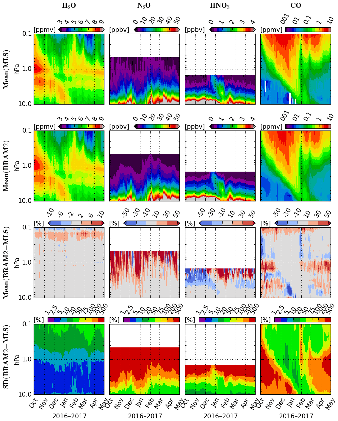
Figure 9Time series of (from top to bottom) daily mean MLS profiles, the corresponding BRAM2 values, the relative mean differences (%) between BRAM2 and MLS, and the associated standard deviation (%). Values are shown between October 2016 and May 2017, between 90 and 60∘ N, and between 0.1 and 10 hPa for (from left to right) H2O, N2O, HNO3 and CO.
Note that CTRL is not shown in this section. It displays large disagreement with MLS and/or BRAM2, which only highlights the CTM limitations explained above.
Figure 9 shows the time series of MLS and BRAM2 during the USPV Arctic winter 2016–2017, between 0.1 and 10 hPa and averaged between 60 and 90∘ N. Note that the figure is not given in the equivalent latitude–theta view as in the LSPV in order to keep the upper model levels in the discussion. This winter was subject to intense dynamical activity with two strong warmings – although not major – where the vortex almost split at the end of January and February (not shown). Around these dates, discontinuities in the time series of MLS H2O and CO are clearly visible and reproduced well by BRAM2. Time series of MLS HNO3 show enhanced values in January around 3 hPa most likely due to ion chemistry. While this process is not included in the BASCOE CTM, BRAM2 agrees well with MLS. The average BRAM2 N2O also agrees well with MLS below 1 hPa.
Figure 9 also displays the relative mean difference and standard deviation between BRAM2 and MLS. As for previous comparisons shown in this paper, the mean and standard deviation are large when the abundance of the species is relatively low, i.e. in the upper parts of the plots for N2O and HNO3, or for CO outside the period of enhancement by descent of mesospheric air. Otherwise, the agreement is relatively good for CO during descent of mesospheric air, during production of HNO3 by ion chemistry or at lower altitude for N2O when its abundance exceeds ∼20 ppbv. In those cases, the bias is around ±10 %, while the standard deviations of the differences are relatively large but still acceptable (<50 %). For H2O the agreement is very good below 0.2 hPa, where bias and standard deviation are usually lower than ±2 % and 20 %, respectively.
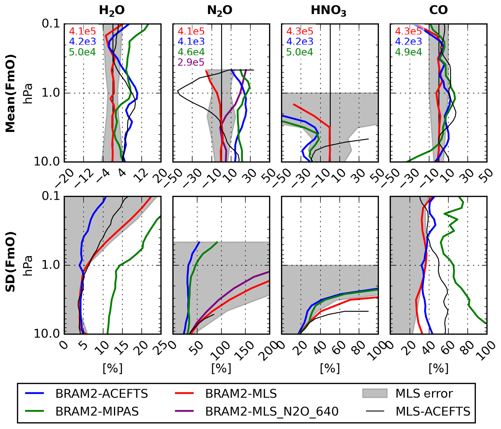
Figure 10Mean (top row) and standard deviation (bottom row) of the differences between BRAM2 and observations from MLS (red lines), ACE-FTS (blue lines), MIPAS (green lines) and MLS_N2O_640 (purple lines). The statistics are in percent, normalized by the mean of BRAM2, and are taken between 60 and 90∘ N, between 0.1 and 10 hPa, and between the months January and February (i.e. during months observed by ACE-FTS) of the period 2005–2017. The statistics are calculated for, from left to right, H2O, N2O, HNO3 and CO. The approximate numbers of observed profiles used in the FmO statistics are given in the upper left corner of the top row plots using the instrument colour code. The grey shaded area in the mean and standard deviation plots corresponds, respectively, to the MLS accuracy and precision, as provided in the MLS data quality document (see L2015). The thin black profiles represent the mean (top row) and standard deviations (bottom row) between MLS and ACE-FTS found in validation publications (see text for details).
Figure 10 shows the FmO statistics between BRAM2 and observations from MLS, ACE-FTS, MIPAS and MLS_N2O_640 in the USPV. These statistics are calculated between 60 and 90∘ N and between 0.1 and 10 hPa for the January–February 2005–2017 periods, these months being observed by ACE-FTS (for MIPAS and MLS_N2O_640, the datasets end in 2012 and 2013, respectively). The figure also shows the MLS accuracy and precision, and the mean and standard deviation of the differences (MLS − ACE-FTS) estimated by S2017. A similar figure for the southern polar winter is provided in the Supplement (Fig. S9).
The FmO statistics are similar to those found in the middle stratosphere (see Fig. 5, Sect. 5.1) for H2O and N2O. FmO statistics for HNO3 are also somewhat similar to those found in the middle stratosphere. The major difference is the smaller bias found in the USPV between BRAM2 and MLS (<5 %) at altitude below 3 hPa, approximately the upper level where HNO3 is produced by ion chemistry, well within the MLS accuracy. The FmO statistics of these three species are also stable from year to year (not shown) and similar values are found in the Southern Hemisphere (see Fig. S9).
For CO, bias against MLS is small ( %) and well within the MLS accuracy. The biases against ACE-FTS or MIPAS are similar, usually within ±10 % with a maximum positive bias of +15 % at 1 hPa. The bias against ACE-FTS agrees well with the direct comparison between MLS and ACE-FTS which suggests that the BRAM2 bias comes from the differences between the two instruments.
The standard deviations of CO against MLS (∼35 %) agree well with the MLS precision. BRAM2 provides similar standard deviations against ACE-FTS which are significantly lower than in the direct comparison between MLS and ACE-FTS. Against MIPAS, the standard deviation is relatively large, between 50 % and 80 %.
In the Southern Hemisphere, the biases against ACE-FTS and MIPAS are slightly larger by ∼5 % and ∼10 %, respectively (see Fig. S9). On the other hand, the standard deviations are smaller by around 10 % against all datasets, with very good agreement with the difference (MLS − ACE-FTS). These statistics are relatively stable over the years. BRAM2 CO in the USPV agrees well with observations and is recommended for scientific use.
5.4 Upper troposphere–lower stratosphere (UTLS))
In the UTLS, the evaluation of BRAM2 must take into account several limitations of the BASCOE CTM and the satellite observations. The BASCOE CTM does not include tropospheric processes, in particular the convection which is necessary to represent correctly vertical transport from the lower to the upper troposphere (Pickering et al., 1996; Folkins et al., 2002). Moreover, the BASCOE spatial resolution used for BRAM2 is relatively coarse to represent vertical and horizontal gradients in this region. Additionally, satellite observations are less reliable in the UTLS because large dynamical variability and steep gradients across the tropopause limit instruments with low temporal (occultation sounders such as ACE-FTS) or vertical (emission sounders such as MLS and MIPAS) resolution. Also, cloud interference and saturation of the measured radiances pose challenges to the instruments, depending on the measurement mode applied (SPARC, 2017).
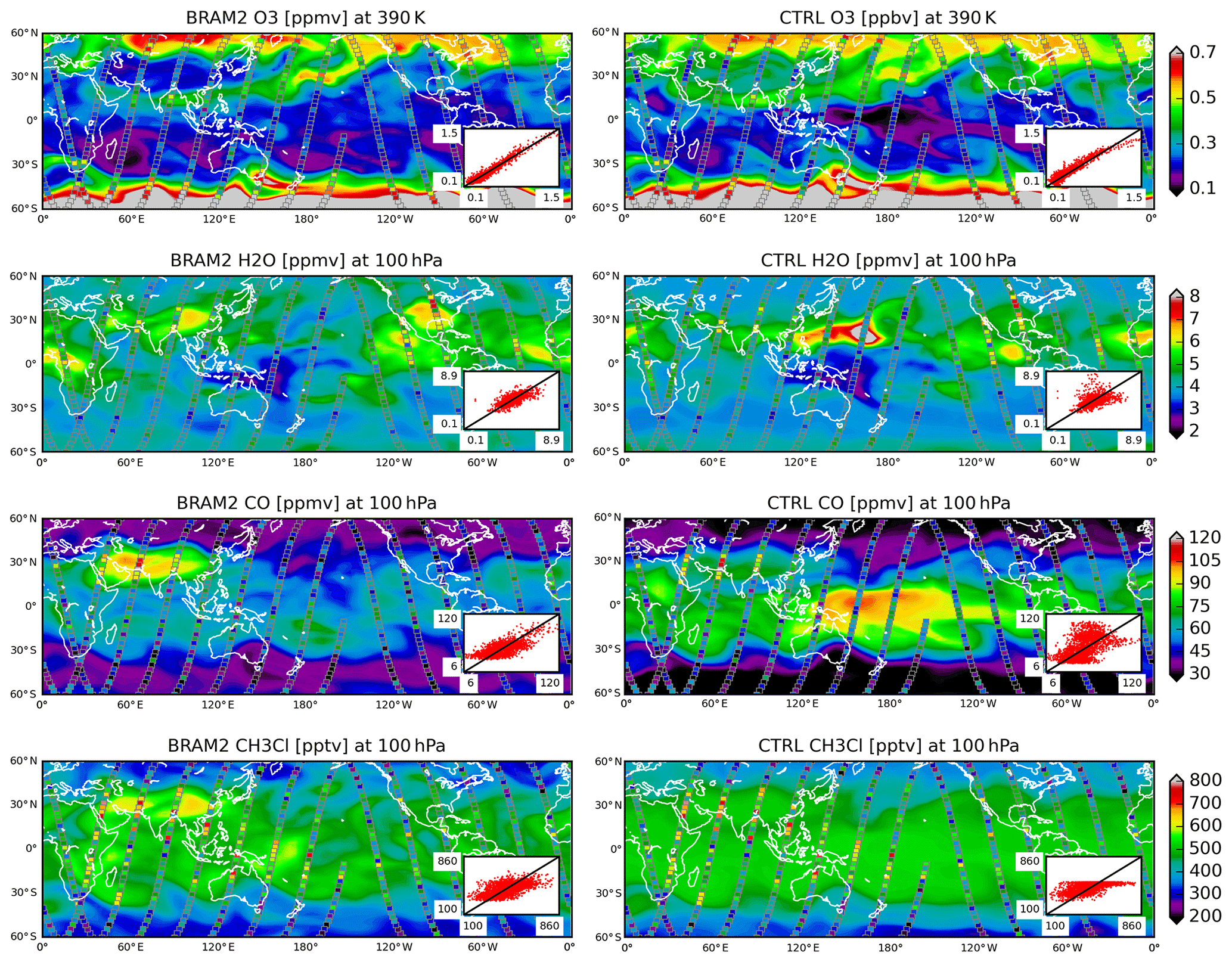
Figure 11The filled contour maps (between 60∘ S and 60∘ N) show the BRAM2 (left column) and CTRL (right column) distribution of, from top to bottom, O3, H2O, CO and CH3Cl on 14 July 2009 at 12:00 UT at 390 K (O3) or 100 hPa (H2O, CO and CH3Cl). Coloured squares correspond to the MLS values between 06:00 and 18:00 UT on that date at the same levels. To improve the readability, only one in two MLS observations is shown. Scatter plots in the lower right corner of each map show the correlation between MLS and BASCOE (BRAM2 or CTRL, MLS on the x axis, BASCOE on the y axis) where all MLS data for that day are used, where BASCOE values are taken from the ModAtObs files (see Sect. 3.4) and where the black lines show the perfect correlation.
In this section, the following BRAM2 species will be evaluated: O3, H2O, CO and CH3Cl. Figure 11 shows the horizontal distribution of these species in the lower stratosphere from BRAM2 and CTRL on 14 July 2009 at 12:00 UT. To highlight the added value of the assimilation, MLS data between 06:00 and 18:00 UT on the same date are overplotted on each map. Finally, the qualitative agreement between MLS and the BASCOE values – BRAM2 or CTRL – corresponding to the selected situation is plotted in the lower right corner of each map. Ozone is shown at 390 K (∼80 hPa in the tropics, ∼150 hPa in mid-latitudes) while the other species are shown at 100 hPa. Despite the BASCOE model limitations, BRAM2 and MLS are in good agreement for O3 (also confirmed by the high correlation between MLS and BRAM2 shown in the figure). For H2O, CH3Cl and CO, the agreement is also generally good although the correlation between MLS and BRAM2 is less compact compared to O3.
During boreal summer, the lower stratosphere is influenced by the anticyclonic circulation located above Asia, which is associated with the Asian summer monsoon (e.g. Randel and Jensen, 2013). In BRAM2 (see Fig. 11), which agrees relatively well with MLS in this region, the anticyclone is marked by low O3 abundance and high abundances of H2O, CO and CH3Cl above Asia, indicating air of tropospheric origin. Also related to the Asian summer monsoon anticyclone is transport from mid-latitudes to the tropics. This transport is marked by the O3 tongue (values ∼400 ppbv) in BRAM2 starting in the northeastern Pacific and ending above India, which denotes air of stratospheric origin around the eastern flank of the anticyclone (Randel and Jensen, 2013, their Fig. 4, although for a different year). Processes related to stratospheric chemistry are relatively well reproduced by CTRL, such as this ozone tongue. This is not the case for tropospheric processes where CTRL shows large disagreement against MLS in the Asian summer monsoon region or over the western Pacific in the tropics.
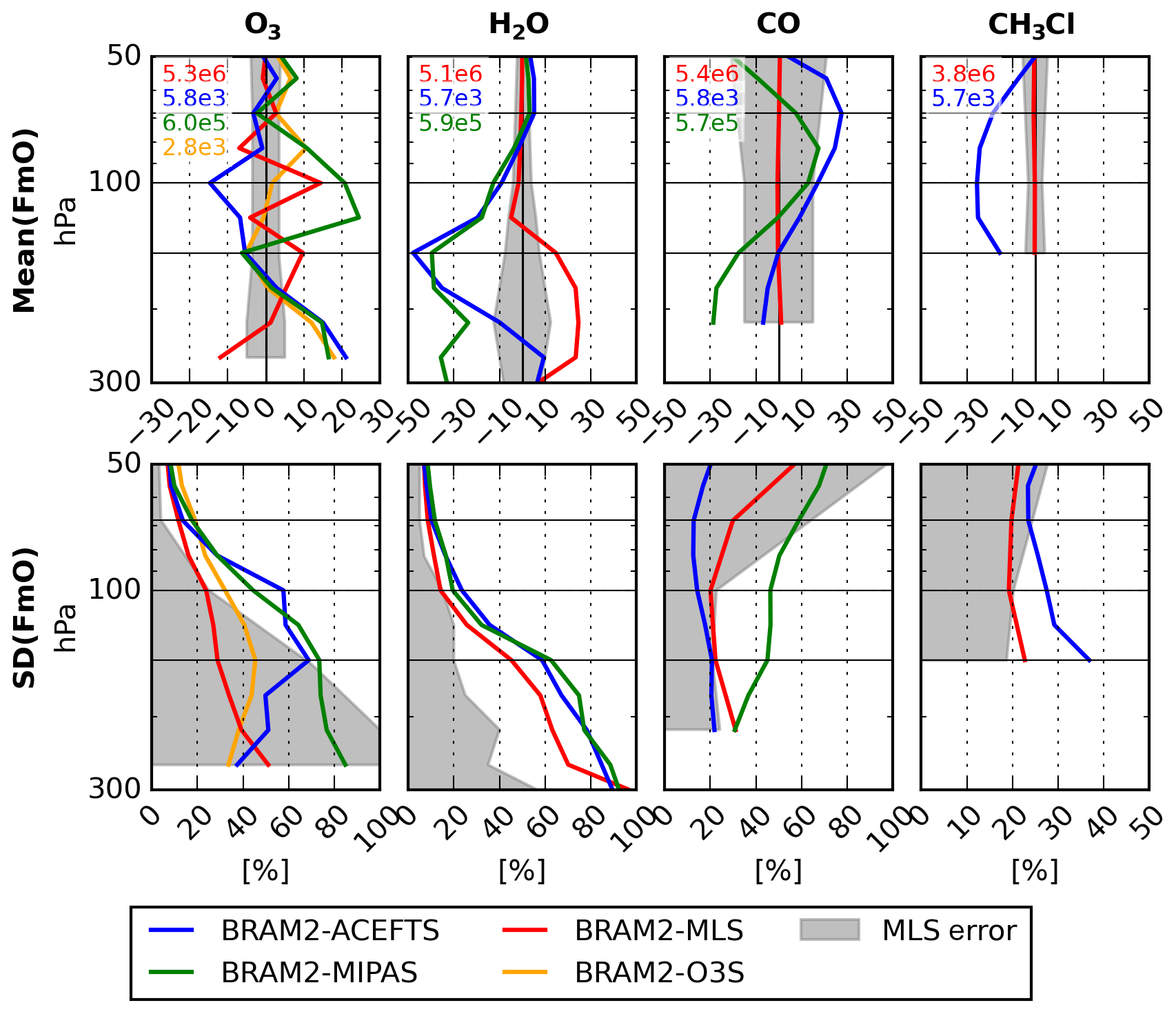
Figure 12Mean (top row) and standard deviation (bottom row) of the differences between BRAM2 and observations from MLS (red lines), ACE-FTS (blue lines), MIPAS (green lines) and NDACC ozonesondes (orange lines). The statistics are in percent, normalized by the mean of BRAM2, and are taken between 30∘ S and 30∘ N, between 50 and 300 hPa, and between 2005 and 2017. The statistics are calculated for, from left to right, O3, H2O, CO and CH3Cl. The approximate numbers of observed profiles used in the FmO statistics are given in the upper left corner of the top row plots using the instrument colour code. The grey shaded area in the mean and standard deviation plots corresponds, respectively, to the MLS accuracy and precision, as provided in the MLS data quality document (see L2015). The horizontal black lines denote levels where time series are shown in Fig. 13.
Figure 12 shows the FmO statistics between BRAM2 and observations from MLS, ACE-FTS, MIPAS and ozonesondes in the tropical UTLS, or the tropical tropopause layer (TTL), for the 2005–2017 period (2005–2012 for MIPAS). The figure also shows the MLS error budget (accuracy and precision). The differences between MLS and ACE-FTS derived from validation papers (S2017 for O3 and H2O; Santee et al. (2013) for CH3Cl) are not shown as is the case in the MS and USPV sections, due to the lack of coincident profiles between the two instruments in the tropics. Figure 12 is complemented by Fig. 13 showing time series of the mean differences of the FmO and the standard deviation against ACE-FTS or ozonesondes (for O3 ). Table 3 provides FmO statistics at three typical levels of the TTL for the period 2005–2017. The results for each species are discussed individually below with a focus on the TTL. FmO values in the extra-tropical UTLS (ex-UTLS) are provided in the Supplement (see Figs. S10–S13 and Table S1).
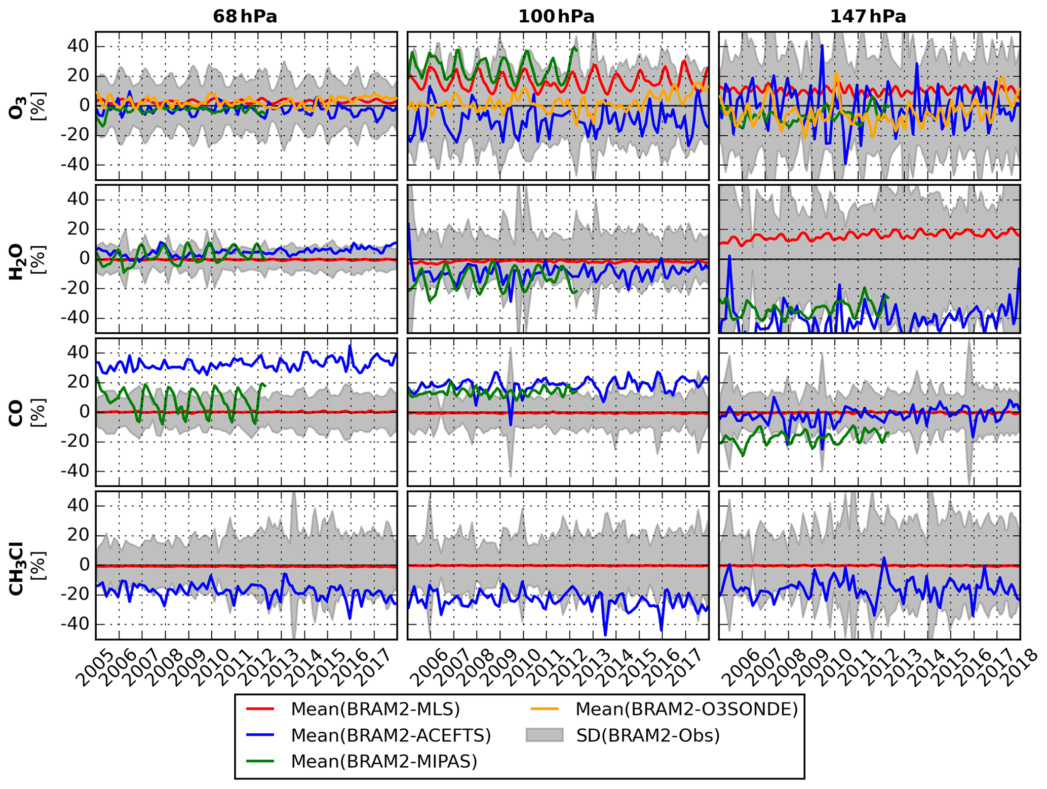
Figure 13Time series of the monthly mean differences between BRAM2 and the different observational datasets in the TTL (30∘ S–30∘ N) at three pressure levels (from left to right: 68, 100 and 147 hPa) and for (top to bottom) O3, H2O, CO and CH3Cl. Values are in percent. The grey shaded area represents the standard deviation of the differences between BRAM2 and ACE-FTS except for O3 where ozonesonde data are used.
O3. In the TTL, the bias profile against MLS oscillates (Fig. 12), due to vertical oscillations in the MLS profiles (Yan et al., 2016, see L2015). The vertical resolution of BASCOE and MLS being similar in the TTL for O3, the system cannot find a state that simultaneously minimizes the difference against all values of the MLS profiles, and it delivers a vertically smoother reanalysis. Because of these oscillations, the bias against MLS is larger than the MLS accuracy. Nevertheless, the bias against independent observations is relatively small, in particular against ozonesondes. Note that satellite observations of O3 in the TTL show a large climatological uncertainty and SPARC (2017) recommends the use of in situ observations. Note also the similar disagreement between BRAM2 and the independent observations from ACE-FTS, MIPAS and ozonesondes below 150 hPa. This suggests good agreement between these three observational datasets and a positive bias in MLS O3. Standard deviation of the differences is small against all observations above 70 hPa (<20 %) and increases to values between 35 % and 80 % in the troposphere, depending on the instruments. Considering the limitations of BRAM2 and the satellite observations mentioned above, this level of agreement is satisfactory.
Time series of the biases against MLS are stable even though they show seasonal variations (see Fig. 13), with the highest amplitude being found at 100 hPa (∼15 %). The difference with independent observations is small at 68 hPa and increases at lower altitude. In all cases, the agreement against ozonesondes is better than ±15 %. This is satisfactory considering the higher representativeness of ozonesondes against BRAM2.
In the ex-UTLS, the agreement with MLS and independent observations is even better; in particular the agreement with MLS is within the MLS uncertainty (see Figs. S10–S13 and Table S1). Considering the low abundance of O3 in the UTLS and the limitations of BASCOE and satellite measurements in this region, we found good agreement between BRAM2 and independent observations. Overall, we recommend BRAM2 O3 in this region for scientific use.
H2O. In the TTL and above the tropopause (approximately 100 hPa in the TTL), BRAM2 agrees well with MLS, ACE-FTS and MIPAS (see Fig. 12 and Table 3). Below that level, the FmO statistics are larger where BRAM2 underestimates ACE-FTS and MIPAS and overestimates MLS. FmO statistics against ACE-FTS and MIPAS are similar above 200 hPa, suggesting a high bias between MLS and these two instruments. On the other hand, comparisons between MLS and in situ cryogenic frost point hygrometer (CFH) observations display similar bias profiles to those between MLS and BRAM2 (Vömel et al., 2007; Yan et al., 2016, respectively their Figs. 6 and 8). This suggests that BRAM2 is closer to in situ CFH observations in the upper troposphere, with MLS being too dry and ACE-FTS and MIPAS being too wet.
Time series of the FmO statistics are relatively stable (no drifts) at 68 and 100 hPa in the TTL (see Fig. 13). At 147 hPa, the bias against MLS increases (from ∼10 % in 2005 to ∼15 % in 2018) with small seasonal variations (amplitude around 5 %). The bias against ACE-FTS shows larger variability, probably due to the low sampling of ACE-FTS in the tropics. Against MIPAS, the biases are large at each level, with seasonal variations around 20 %.
Similar FmO statistics are found in the ex-UTLS (see Figs. S10–S13 and Table S1). Overall, above the tropopause, we recommend BRAM2 H2O for scientific use. In the upper troposphere BRAM2 overestimates MLS and underestimates ACE-FTS and MIPAS and seems to be in good agreement with CFH observations. Nevertheless, the standard deviations of the differences are large in the upper troposphere, and below the tropopause BRAM2 H2O should not be used without consulting the BASCOE team.
CO. BRAM2 agrees well with MLS (Fig. 12 and Table 3) in the TTL, within the MLS accuracy and precision. The bias against ACE-FTS and MIPAS shows similar profiles where BRAM2 displays a negative bias in the upper troposphere and a positive bias in the lower stratosphere against these two instruments. Although showing similar profiles, ACE-FTS seems to measure more CO than MIPAS, between 5 % and 20 %, depending on the altitudes.
There are no drifts or seasonal variations in the time series of the bias against MLS (Fig. 13). For ACE-FTS, the time series are noisy, without clear seasonal variations, probably due to the poor sampling of this instrument in the TTL. For MIPAS, the time series are also noisy at 100 and 147 hPa, while at 68 hPa it displays a clear seasonal variation with a 25 % amplitude. Since the retrieval of MIPAS CO is carried out in log-space, their AKs are vmr-dependent such that their use in the comparison with BRAM2 would have reduced the apparent discrepancies. The impact of MIPAS AKs for CO has not been tested and is left for future comparison.
In the ex-UTLS, the agreement of BRAM2 with MLS is similar to that in the TTL while the biases against ACE-FTS and MIPAS are shifted by around +25 % and display larger seasonal variations (see Figs. S10–S13 and Table S1). Nevertheless, BRAM2 CO is well characterized in the UTLS and we recommend the product for scientific use.
Table 3Mean difference and standard deviation between BRAM2 and observations for the 2005–2017 period at three typical levels in the TTL: 68, 100 and 147 hPa. Values are in percent, normalized by BRAM2. Abbreviations: not assimilated (N.A.).

CH3Cl. In the TTL, BRAM2 agrees well with MLS (Fig. 12 and Table 3), within the MLS accuracy and precision. BRAM2 underestimates ACE-FTS, within −25 % to −15 %. There are no drifts or seasonal variations in the time series of the bias against MLS (Fig. 13), while comparisons with ACE-FTS are noisy with a small noticeable drift at 68 and 100 hPa (the origin of this drift, from MLS or ACE-FTS measurements, has not been identified). Similar conclusions hold in the ex-UTLS (see Figs. S10–S13 and Table S1). Excluding trend studies, we recommend BRAM2 CH3Cl in the TTL for scientific use.
5.5 Summary of the evaluation
The evaluation of BRAM2 is based on the comparison against assimilated MLS data and independent observations from ACE-FTS, MIPAS, MLS_N2O_640, SMILES ClO and NDACC ozonesondes. The evaluation has been performed in four regions: the middle stratosphere (MS), the lower-stratospheric polar vortex (LSPV), the upper-stratospheric–lower-mesospheric polar vortex (USPV) and the tropical tropopause layer (TTL).
In general, the mean differences between BRAM2 and MLS are negligible and within the MLS accuracy. The standard deviations of the differences are also generally within the MLS precision, except for O3 in the MS. This means that in general, BRAM2 can be considered a proxy for MLS. Each species is discussed individually below. The vertical range of validity of BRAM2 in the four evaluated regions is given in Table 4.
Table 4Vertical ranges of validity (hPa) of MLS v4 assimilated species and the corresponding BRAM2 products in the middle stratosphere (MS), the lower-stratospheric polar vortex (LSPV), the upper-stratospheric–lower-mesospheric polar vortex (USPV) and the tropical tropopause layer (TTL). Abbreviations: not evaluated (N.E.) and not assimilated (N.A.).
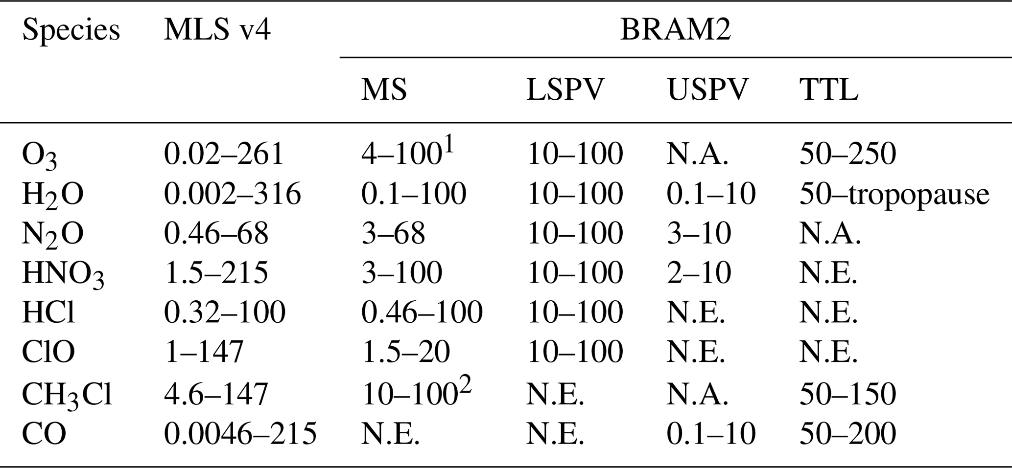
1 O3 has not been assimilated above 4 hPa (see text for details). Above that level, BRAM2 O3 has not been evaluated and should not be used. 2 In the tropics. At mid-latitudes, the vertical range is 30–100 hPa.
O3. Ozone has been evaluated in the MS, LSPV and UTLS. The BASCOE CTM has an ozone deficit around 1 hPa (−20 % vs. MLS; Skachko et al., 2016), which is also present in other models (SPARC, 2010, see their Fig. 6.17). For this reason, MLS O3 has not been assimilated (and has not been evaluated) at altitude above (i.e. pressure lower than) 4 hPa. With the exception of the TTL, BRAM2 agrees well with MLS (±5 %), ACE-FTS (±5 %), MIPAS (−8 % to 5 %) and ozonesondes (±10 %), with substantial changes in the values depending on the region of interest. In the TTL, MLS O3 profiles display unphysical oscillations that are smoothed in BRAM2, with an agreement against ozonesondes generally better than ±10 %. In the upper troposphere BRAM2 underestimates MLS by around 10 % at 260 hPa and overestimates ACE-FTS, MIPAS and ozonesondes by around 20 % at 260 hPa. This suggests that MLS has a positive bias against the three other instruments.
H2O. Water vapour has been evaluated in all four regions. Between the tropopause and the model lid (0.1 hPa), BRAM2 H2O agrees very well with MLS (±2 %) and ACE-FTS (±10 %). Except in the LSPV, the agreement with MIPAS is also good (better than ±10 %). In the LSPV, a larger bias against MIPAS is found that could be reduced by using the MIPAS averaging kernels in the comparison. Below the tropical tropopause, BRAM2 has a positive bias against MLS (around 25 %) and a negative bias against ACE-FTS and MIPAS (around −30 % at 178 hPa). On the other hand MLS underestimates in situ cryogenic frost point hygrometer (CFH; Vömel et al., 2007; Yan et al., 2016) observations by around 25 %, which suggests a good agreement between BRAM2 and CFH as well as a positive bias of ACE-FTS and MIPAS against CFH.
N2O. Nitrous oxide has been evaluated in the MS, LSPV and USPV. BRAM2 is well characterized by comparison against independent observations at altitudes below (i.e. pressures larger than) 3 hPa. In the MS, BRAM2 agrees well with MLS (±1 %), ACE-FTS (±10 %), MIPAS (±15 %) and MLS_N2O_640 (±5 %). Above that level, BRAM2 is poorly characterized by comparison against observations where time series of mean differences are noisy. In conditions of low abundance of N2O encountered during the subsidence of the polar vortex (LSPV and USPV), BRAM2 overestimates independent observations but unnormalized differences are generally small. This study reveals a negative drift between BRAM2 and the three independent observational datasets, which suggests a negative drift in the MLS N2O standard product. This issue is under investigation by the MLS team (Livesey et al., 2019).
HNO3. Nitric acid has been evaluated in the MS, LSPV and USPV. BRAM2 is well characterized by comparison against independent observations below 3 hPa. Below 10 hPa, BRAM2 agrees well against MLS (±2 %), ACE-FTS and MIPAS (−10 % to 1 % in both cases). From 10 to 3 hPa, the mean differences grow (±10 % against MLS) and exceed ±50 % above 2 hPa for the three datasets. Above that level, MLS precision degrades (to around 0.6 ppbv, i.e. 6 times the typical amount of HNO3 at that level), and the constraint by the assimilated observations on BASCOE is weak. In the polar vortex after denitrification, BRAM2 has a small negative bias against independent observations (−5 %). Despite the lack of ion chemistry and sources of mesospheric NOx in BASCOE, enhanced HNO3 in the USPV is well represented in BRAM2.
HCl. Hydrogen chloride has been evaluated in the MS and LSPV. BRAM2 agrees well with ACE-FTS in MS between 0.4 and 100 hPa at mid-latitudes and between 0.4 and 50 hPa in the tropics. At altitude above 5 hPa, MLS HCl drifts (see Sect. 5.1 for details), which results in a positive drift in the comparison between BRAM2 and ACE-FTS. In the LSPV when HCl is completely depleted by heterogeneous chemistry on PSCs, BRAM2 has a positive bias against independent observations, which remains small when the unnormalized bias is considered (<0.2 ppbv).
ClO. Chlorine monoxide has been evaluated in the MS and the LSPV. In the MS, BRAM2 agrees well with independent observations even though it is poorly constrained by MLS observations. The constraint of MLS observations is stronger in LSPV under conditions of chlorine activation, when BRAM2 agrees well with independent observations.
CH3Cl. Methyl chloride has been evaluated in the MS and the UTLS. At altitudes below 10 hPa in the tropics and 30 hPa in the mid-latitudes, BRAM2 agrees very well with MLS (±5 %). The agreement is good with ACE-FTS in the tropics (±20 %) and less good at mid-latitudes (−60 % to 20 %). Above these altitudes, BRAM2 has a positive bias against MLS, likely because the averaging kernels of MLS are not used. BRAM2 agrees well with MLS (±1 %) and ACE-FTS (−25 % to −15 %) in the UTLS.
CO. Carbon monoxide has been evaluated in the USPV and the UTLS. In the USPV, during descent of mesospheric CO, BRAM2 agrees well with MLS (±5 %) and independent observations (typically 10 % against ACE-FTS and MIPAS). In the UTLS, the bias between BRAM2 and MLS is negligible (±2 %). BRAM2 agrees reasonably well with ACE-FTS and MIPAS in the TTL: typical biases are, respectively, 25 % and 18 % around 70 hPa to −8 % and −30 % at 215 hPa. In the ex-UTLS, biases against ACE-FTS and MIPAS are shifted by around +20 % and display larger seasonal variations.
According to the evaluation of BRAM2 with MLS and independent observations, we recommend scientific use of BRAM2 with the following limitations. The use of BRAM2 species should be restricted to their evaluated regions (see Table 4). In the MS, O3, N2O and HNO3 should be used at altitude below, respectively, 4, 3 and 3 hPa. BRAM2 N2O and HCl should be excluded from any trend studies. Methyl chloride should be used below 10 hPa in the tropics and 30 hPa at mid-latitudes. In the tropics at altitudes below 50 hPa, BRAM2 HCl can be used with the caveat of a positive bias with respect to independent observations.
5.6 Note on the BRAM2 unobserved species
The above evaluation focuses on the eight species constrained by MLS observations while BRAM2 includes many others. Although it is beyond the scope of this paper, one can ask what is the value of BRAM2 unobserved species. For long-lived species (e.g. methane or the chlorofluorocarbons), small discontinuities appear in the troposphere at the stream transitions. This is due to the fact that each stream is initialized by a 20-year simulation with time-dependent emissions of tropospheric source gases (see Sect. 3.2) while emissions are kept constant during the stream productions. For short-lived species, the impact is mixed. For example, we found an improvement from CTRL to BRAM2 NO2 when compared to MIPAS or ACE-FTS in the lower stratosphere but a degradation in the upper stratosphere. Except for Cl2O2, which is closely related to ClO during the chlorine activation period, BRAM2 unobserved species are not delivered.
This paper presents a new reanalysis of stratospheric composition produced by the Belgian Assimilation System of Chemical ObsErvations (BASCOE). It is based on the assimilation of measurements from the Microwave Limb Sounder (MLS), on board the Aura satellite, of namely O3, H2O, N2O, HNO3, HCl, ClO, CH3Cl and CO. BRAM2 (BASCOE Reanalysis of Aura MLS version 2) covers the period 2004–2017 and will be extended in the future. The reanalysis is evaluated by comparison with independent observations from ACE-FTS, MIPAS, MLS_N2O_640 (i.e. N2O retrieved from the MLS 640 GHz radiometer until 2013), SMILES ClO and NDACC ozonesondes. The evaluation of BRAM2 has been carried out in four regions: the middle stratosphere (MS), the lower-stratospheric polar vortex (LSPV), the upper-stratospheric–lower-mesospheric polar vortex (USPV) and the upper troposphere–lower stratosphere (UTLS). Only species which are relevant in the selected region have been evaluated. Moreover, while the BASCOE model includes 58 chemical species, only those constrained by the assimilated MLS species have been evaluated. Finally, the analysis uncertainties based on the standard deviation of the ensemble state have not been evaluated in this paper. It will be the subject of a future study.
BRAM2 is well characterized by comparison against independent observations and is in most cases recommended for scientific use. One important limitation is reported here: the BASCOE model, as other models, suffers from an ozone deficit around 1 hPa where it underestimates MLS by ∼20 %. Since the lifetime of O3 at these altitudes is shorter than the revisit time of MLS, approximately 12 h between an ascending and a descending orbit, data assimilation cannot correct this bias. MLS O3 profiles have thus not been assimilated (and have not been evaluated) at altitudes above (i.e. at pressures lower than) 4 hPa. Above that level BRAM2 O3 should not be used.
The mean and standard deviation of the difference between BRAM2 and ACE-FTS have been compared to the differences between collocated profiles of MLS and ACE-FTS provided in published validation studies (namely Froidevaux et al., 2008b; Sheese et al., 2017; Santee et al., 2013). The mean differences are in general similar, which means that most of the differences between BRAM2 and the independent observations are due to the differences between these datasets and MLS. The standard deviations of the difference (BRAM2 − ACE-FTS) are usually as good as or better than those from (MLS − ACE-FTS). This suggests that the representativeness errors within BRAM2 are smaller than the sampling errors inherent in validation studies based on collocation of profiles.
A BASCOE control run (no assimilation, denoted CTRL) initialized by BRAM2 has been run for several months (between May 2009 and November 2010) to assess the added value of the assimilation compared to a pure model run. Spatial gradients across dynamical barriers are improved in BRAM2 with respect to CTRL. The representation of the LSPV in the presence of PSCs is also improved, in particular for H2O, HCl and ClO. Subsidence in the polar vortex is improved thanks to the assimilation. The BASCOE system does not include mesospheric sources of CO, H2O or NOx or ion chemistry to account for the formation of HNO3 in polar winters. Nevertheless, the MLS observations provide a sufficient constraint to correct for these model biases. The BASCOE model also lacks detailed tropospheric processes (chemistry, washout, convection), and, again, the MLS data provide a sufficient constraint to correct for these biases.
BRAM2 also adds value to the observations. MLS O3 profiles display unphysical oscillations in the tropical UTLS which are smoothed in BRAM2, in good agreement with independent observations. It also allowed us to identify a positive drift in the MLS N2O standard product, retrieved from the 190 GHz radiometer in the v4 MLS retrieval, against measurements from ACE-FTS, MIPAS or MLS_N2O_640. Since BRAM2 is usually not biased against MLS, this reanalysis could be used to study the biases between MLS and other instruments. In the upper troposphere, the comparison of BRAM2 with MLS and independent observations suggests that MLS O3 is overestimated and MLS H2O is underestimated.
This study also indicates several directions to improve the reanalysis for future versions. The first one is to increase the spatial resolution and to improve several processes in the BASCOE CTM, in particular the convection and the PSC microphysical scheme. Improving the photochemical scheme for O3 could reduce the BASCOE ozone deficit. We believe that short-lived species, like O3 around 1 hPa or ClO in the middle stratosphere, should not be assimilated. For ozone above 4 hPa, a better approach would be to use EnKF and MLS observations to optimize model parameters that control the abundance of ozone in this region. Such a method still needs to be developed. Including realistic upper boundary conditions for CO, H2O and NOx, as well as implementing ion chemistry, would improve the system to represent the USPV region. Implementing the use of the averaging kernels would improve the analysis for CH3Cl at mid-latitudes. It would also improve the comparison against independent observations like MIPAS H2O in the UTLS and in polar winter conditions. Bias correction to remove the vertical oscillations in the MLS O3 profiles and to remove drift in H2O, N2O and HCl would also improve the analysis. Additional observations could also be considered as long as they add value to MLS and they do not introduce spurious discontinuities. Ozone profiles from the Ozone Climate Change Initiative could also be considered as long as their biases are removed, which has not yet been done (Hubert et al., 2016). Total ozone column observations provided by the Ozone Climate Change Initiative (Lerot et al., 2014), based on several nadir sounders but free of bias and with a total period covering 1995–present, would allow one to provide the total ozone column and probably improve tropospheric ozone analyses. Occultation sounders have a spatial and temporal sampling which is too sparse to constrain a data assimilation system and would be used for the evaluation of the analyses. Other research limb instruments (e.g. MIPAS) could be considered but preliminary tests should first demonstrate that their spatial and temporal sampling is sufficiently continuous to preserve the stability of the reanalysis.
BRAM2 is available to the scientific community and will be extended to later years observed by MLS in the near future.
BRAM2 6-hourly gridded outputs are freely available to registered users on the BIRA-IASB ftp site. Only the MLS assimilated species plus Cl2O2 are available. Access information is available at http://strato.aeronomie.be/index.php/2-uncategorised/6-bram (Errera, 2019). BRAM2 ModAtObs files (see Sect. 3.4) are available upon request to the BASCOE team (quentin.errera@aeronomie.be).
The supplement related to this article is available online at: https://doi.org/10.5194/acp-19-13647-2019-supplement.
QE led the development of the BASCOE data assimilation system, designed the configuration for BRAM2, realized its evaluation, produced the figures and wrote most of the text. SC, YC, JD and SS contributed to the development of BASCOE. MLS, KW, DH and MS contributed to the writing of the section dealing with the observations from, respectively, MLS, ACE-FTS, ozonesondes and SMILES. All authors reviewed the paper before submission.
The authors declare that they have no conflict of interest.
The Atmospheric Chemistry Experiment, also known as SCISAT, is a Canadian-led mission mainly supported by the CSA and NSERC. The ozonesonde data used in this publication were obtained from the Network for the Detection of Atmospheric Composition Change (NDACC) and are publicly available (see http://www.ndacc.org, last access: 6 November 2019). We thank Bavo Langerok for preprocessing the ozonesonde data in the HDF-5 GEOMS format. Work at the Jet Propulsion Laboratory, California Institute of Technology, was carried out under contract with the National Aeronautics and Space Administration. Thanks to Farahnaz Khosrawi, Stefan Lossow, Michael Kiefer and Norbert Glatthor for helpful discussions on MIPAS data. Thanks also to Richard Ménard for helpful discussions about the EnKF method. Quentin Errera also dedicates this work to his friend William Lahoz, who passed away in April 2019.
This paper was edited by Jens-Uwe Grooß and reviewed by three anonymous referees.
Akiyoshi, H., Nakamura, T., Miyasaka, T., Shiotani, M., and Suzuki, M.: A nudged chemistry-climate model simulation of chemical constituent distribution at northern high-latitude stratosphere observed by SMILES and MLS during the 2009/2010 stratospheric sudden warming, J. Geophys. Res.-Atmos., 121, 1361–1380, https://doi.org/10.1002/2015JD023334, 2016. a
Anderson, E. and Järvinen, H.: Variational quality control, Q. J. Roy. Meteor. Soc., 125, 697–722, https://doi.org/10.1002/qj.49712555416, 1999. a
Bernath, P. F., McElroy, C. T., Abrams, M. C., Boone, C. D., Butler, M., Camy-Peyret, C., Carleer, M., Clerbaux, C., Coheur, P.-F., Colin, R., DeCola, P., DeMazière, M., Drummond, J. R., Dufour, D., Evans, W. F. J., Fast, H., Fussen, D., Gilbert, K., Jennings, D. E., Llewellyn, E. J., Lowe, R. P., Mahieu, E., McConnell, J. C., McHugh, M., McLeod, S. D., Michaud, R., Midwinter, C., Nassar, R., Nichitiu, F., Nowlan, C., Rinsland, C. P., Rochon, Y. J., Rowlands, N., Semeniuk, K., Simon, P., Skelton, R., Sloan, J. J., Soucy, M.-A., Strong, K., Tremblay, P., Turnbull, D., Walker, K. A., Walkty, I., Wardle, D. A., Wehrle, V., Zander, R., and Zou, J.: Atmospheric Chemistry Experiment (ACE): Mission overview, Geophys. Res. Lett., 32, L15S01, https://doi.org/10.1029/2005GL022386, 2005. a
Boone, C. D., Nassar, R., Walker, K. A., Rochon, Y., McLeod, S. D., Rinsland, C. P., and Bernath, P. F.: Retrievals for the Atmospheric Chemistry Experiment Fourier-Transform Spectrometer, Appl. Optics, 44, 7218–7231, https://doi.org/10.1364/AO.44.007218, 2005. a
Boone, C. D., Walker, K. A., and Bernath, P. F.: Version 3 Retrievals for the Atmospheric Chemistry Experiment Fourier Transform Spectrometer (ACE-FTS), in: The Atmospheric Chemistry Experiment ACE at 10: A Solar Occultation Anthology, 103–127, A. Deepak Publishing, Hampton, Virginia, USA, 2013. a
Braathen, G.: Arctic Ozone Bulletin, Tech. Rep. 1, WMO, https://doi.org/10.13140/RG.2.1.4929.6403, 2016. a
Burkholder, J. B., Sander, S. P., Abbatt, J., Barker, J. R., Huie, R. E., Kolb, C. E., Kurylo, M. J., Orkin, V. L., Wilmouth, D. M., and Wine, P. H.: Chemical Kinetics and Photochemical Data for Use in Atmospheric Studies, Evaluation No. 18, Tech. rep., JPL Publication 15-10, Jet Propulsion Laboratory, Pasadena, available at: http://jpldataeval.jpl.nasa.gov (last access: 6 November 2019), 2011. a
Chabrillat, S., Vigouroux, C., Christophe, Y., Engel, A., Errera, Q., Minganti, D., Monge-Sanz, B. M., Segers, A., and Mahieu, E.: Comparison of mean age of air in five reanalyses using the BASCOE transport model, Atmos. Chem. Phys., 18, 14715–14735, https://doi.org/10.5194/acp-18-14715-2018, 2018. a
Charlton, A. J. and Polvani, L. M.: A New Look at Stratospheric Sudden Warmings. Part I: Climatology and Modeling Benchmarks, J. Climate, 20, 449–469, https://doi.org/10.1175/JCLI3996.1, 2007. a
Considine, D. B., Douglass, A. R., Connell, P. S., Kinnison, D. E., and Rotman, D. A.: A polar stratospheric cloud parameterization for the global modeling initiative three-dimensional model and its response to stratospheric aircraft, J. Geophys. Res., 105, 3955–3973, https://doi.org/10.1029/1999JD900932, 2000. a
Davis, S. M., Rosenlof, K. H., Hassler, B., Hurst, D. F., Read, W. G., Vömel, H., Selkirk, H., Fujiwara, M., and Damadeo, R.: The Stratospheric Water and Ozone Satellite Homogenized (SWOOSH) database: a long-term database for climate studies, Earth Syst. Sci. Data, 8, 461–490, https://doi.org/10.5194/essd-8-461-2016, 2016. a
Dee, D. P., Uppala, S. M., Simmons, A. J., Berrisford, P., Poli, P., Kobayashi, S., Andrae, U., Balmaseda, M. A., Balsamo, G., Bauer, P., Bechtold, P., Beljaars, A. C. M., van de Berg, L., Bidlot, J., Bormann, N., Delsol, C., Dragani, R., Fuentes, M., Geer, A. J., Haimberger, L., Healy, S. B., Hersbach, H., Hólm, E. V., Isaksen, L., Kållberg, P., Köhler, M., Matricardi, M., McNally, A. P., Monge-Sanz, B. M., Morcrette, J.-J., Park, B.-K., Peubey, C., de Rosnay, P., Tavolato, C., Thépaut, J.-N., and Vitart, F.: The ERA-Interim reanalysis: configuration and performance of the data assimilation system, Q. J. Roy. Meteor. Soc., 137, 553–597, https://doi.org/10.1002/qj.828, 2011. a
Deshler, T., Stübi, R., Schmidlin, F. J., Mercer, J. L., Smit, H. G. J., Johnson, B. J., Kivi, R., and Nardi, B.: Methods to homogenize electrochemical concentration cell (ECC) ozonesonde measurements across changes in sensing solution concentration or ozonesonde manufacturer, Atmos. Meas. Tech., 10, 2021–2043, https://doi.org/10.5194/amt-10-2021-2017, 2017. a
Desroziers, G., Berre, L., Chapnik, B., and Poli, P.: Diagnosis of observation, background and analysis-error statistics in observation space, Q. J. Roy. Meteor. Soc., 131, 3385–3396, https://doi.org/10.1256/qj.05.108, 2005. a
Errera, Q.: BRAM2 website access, available at: http://strato.aeronomie.be/index.php/2-uncategorised/6-bram, last access: 6 November 2019. a
Errera, Q. and Ménard, R.: Technical Note: Spectral representation of spatial correlations in variational assimilation with grid point models and application to the Belgian Assimilation System for Chemical Observations (BASCOE), Atmos. Chem. Phys., 12, 10015–10031, https://doi.org/10.5194/acp-12-10015-2012, 2012. a, b
Errera, Q., Daerden, F., Chabrillat, S., Lambert, J. C., Lahoz, W. A., Viscardy, S., Bonjean, S., and Fonteyn, D.: 4D-Var assimilation of MIPAS chemical observations: ozone and nitrogen dioxide analyses, Atmos. Chem. Phys., 8, 6169–6187, https://doi.org/10.5194/acp-8-6169-2008, 2008. a, b, c
Fischer, H., Birk, M., Blom, C., Carli, B., Carlotti, M., von Clarmann, T., Delbouille, L., Dudhia, A., Ehhalt, D., Endemann, M., Flaud, J. M., Gessner, R., Kleinert, A., Koopman, R., Langen, J., López-Puertas, M., Mosner, P., Nett, H., Oelhaf, H., Perron, G., Remedios, J., Ridolfi, M., Stiller, G., and Zander, R.: MIPAS: an instrument for atmospheric and climate research, Atmos. Chem. Phys., 8, 2151–2188, https://doi.org/10.5194/acp-8-2151-2008, 2008. a
Folkins, I., Braun, C., Thompson, A. M., and Witte, J.: Tropical ozone as an indicator of deep convection, J. Geophys. Res., 107, ACH 13-1–ACH 13-10, https://doi.org/10.1029/2001JD001178, 2002. a
Froidevaux, L., Jiang, Y. B., Lambert, A., Livesey, N. J., Read, W. G., Waters, J. W., Browell, E. V., Hair, J. W., Avery, M. A., McGee, T. J., Twigg, L. W., Sumnicht, G. K., Jucks, K. W., Margitan, J. J., Sen, B., Stachnik, R. A., Toon, G. C., Bernath, P. F., Boone, C. D., Walker, K. A., Filipiak, M. J., Harwood, R. S., Fuller, R. A., Manney, G. L., Schwartz, M. J., Daffer, W. H., Drouin, B. J., Cofield, R. E., Cuddy, D. T., Jarnot, R. F., Knosp, B. W., Perun, V. S., Snyder, W. V., Stek, P. C., Thurstans, R. P., and Wagner, P. A.: Validation of Aura Microwave Limb Sounder stratospheric ozone measurements, J. Geophys. Res., 113, D15S20, https://doi.org/10.1029/2007JD008771, 2008a.
Froidevaux, L., Jiang, Y. B., Lambert, A., Livesey, N. J., Read, W. G., Waters, J. W., Fuller, R. A., Marcy, T. P., Popp, P. J., Gao, R. S., Fahey, D. W., Jucks, K. W., Stachnik, R. A., Toon, G. C., Christensen, L. E., Webster, C. R., Bernath, P. F., Boone, C. D., Walker, K. A., Pumphrey, H. C., Harwood, R. S., Manney, G. L., Schwartz, M. J., Daffer, W. H., Drouin, B. J., Cofield, R. E., Cuddy, D. T., Jarnot, R. F., Knosp, B. W., Perun, V. S., Snyder, W. V., Stek, P. C., Thurstans, R. P., and Wagner, P. A.: Validation of Aura Microwave Limb Sounder HCl measurements, J. Geophys. Res.-Atmos., 113, D15S25, https://doi.org/10.1029/2007JD009025, 2008b. a, b, c, d, e, f, g
Froidevaux, L., Anderson, J., Wang, H.-J., Fuller, R. A., Schwartz, M. J., Santee, M. L., Livesey, N. J., Pumphrey, H. C., Bernath, P. F., Russell III, J. M., and McCormick, M. P.: Global OZone Chemistry And Related trace gas Data records for the Stratosphere (GOZCARDS): methodology and sample results with a focus on HCl, H2O, and O3, Atmos. Chem. Phys., 15, 10471–10507, https://doi.org/10.5194/acp-15-10471-2015, 2015. a
Froidevaux, L., Kinnison, D. E., Wang, R., Anderson, J., and Fuller, R. A.: Evaluation of CESM1 (WACCM) free-running and specified dynamics atmospheric composition simulations using global multispecies satellite data records, Atmos. Chem. Phys., 19, 4783–4821, https://doi.org/10.5194/acp-19-4783-2019, 2019. a
Fujiwara, M., Wright, J. S., Manney, G. L., Gray, L. J., Anstey, J., Birner, T., Davis, S., Gerber, E. P., Harvey, V. L., Hegglin, M. I., Homeyer, C. R., Knox, J. A., Krüger, K., Lambert, A., Long, C. S., Martineau, P., Molod, A., Monge-Sanz, B. M., Santee, M. L., Tegtmeier, S., Chabrillat, S., Tan, D. G. H., Jackson, D. R., Polavarapu, S., Compo, G. P., Dragani, R., Ebisuzaki, W., Harada, Y., Kobayashi, C., McCarty, W., Onogi, K., Pawson, S., Simmons, A., Wargan, K., Whitaker, J. S., and Zou, C.-Z.: Introduction to the SPARC Reanalysis Intercomparison Project (S-RIP) and overview of the reanalysis systems, Atmos. Chem. Phys., 17, 1417–1452, https://doi.org/10.5194/acp-17-1417-2017, 2017. a
Funke, B., López-Puertas, M., Gil-López, S., von Clarmann, T., Stiller, G. P., Fischer, H., and Kellmann, S.: Downward transport of upper atmospheric NOx into the polar stratosphere and lower mesosphere during the Antarctic 2003 and Arctic 2002/2003 winters, J. Geophys. Res., 110, D24308, https://doi.org/10.1029/2005JD006463, 2005. a
Funke, B., López-Puertas, M., García-Comas, M., Stiller, G. P., von Clarmann, T., Höpfner, M., Glatthor, N., Grabowski, U., Kellmann, S., and Linden, A.: Carbon monoxide distributions from the upper troposphere to the mesosphere inferred from 4.7 μm non-local thermal equilibrium emissions measured by MIPAS on Envisat, Atmos. Chem. Phys., 9, 2387–2411, https://doi.org/10.5194/acp-9-2387-2009, 2009. a, b
Geer, A. J., Lahoz, W. A., Bekki, S., Bormann, N., Errera, Q., Eskes, H. J., Fonteyn, D., Jackson, D. R., Juckes, M. N., Massart, S., Peuch, V.-H., Rharmili, S., and Segers, A.: The ASSET intercomparison of ozone analyses: method and first results, Atmos. Chem. Phys., 6, 5445–5474, https://doi.org/10.5194/acp-6-5445-2006, 2006. a
Glatthor, N., von Clarmann, T., Fischer, H., Grabowski, U., Höpfner, M., Kellmann, S., Kiefer, M., Linden, A., Milz, M., Steck, T., Stiller, G. P., Mengistu Tsidu, G., Wang, D.-Y., and Funke, B.: Spaceborne ClO observations by the Michelson Interferometer for Passive Atmospheric Sounding (MIPAS) before and during the Antarctic major warming in September/October 2002, J. Geophys. Res., 109, D11307, https://doi.org/10.1029/2003JD004440, 2004. a
Grooß, J.-U., Müller, R., Spang, R., Tritscher, I., Wegner, T., Chipperfield, M. P., Feng, W., Kinnison, D. E., and Madronich, S.: On the discrepancy of HCl processing in the core of the wintertime polar vortices, Atmos. Chem. Phys., 18, 8647–8666, https://doi.org/10.5194/acp-18-8647-2018, 2018. a, b
Hubert, D., Lambert, J.-C., Verhoelst, T., Granville, J., Keppens, A., Baray, J.-L., Bourassa, A. E., Cortesi, U., Degenstein, D. A., Froidevaux, L., Godin-Beekmann, S., Hoppel, K. W., Johnson, B. J., Kyrölä, E., Leblanc, T., Lichtenberg, G., Marchand, M., McElroy, C. T., Murtagh, D., Nakane, H., Portafaix, T., Querel, R., Russell III, J. M., Salvador, J., Smit, H. G. J., Stebel, K., Steinbrecht, W., Strawbridge, K. B., Stübi, R., Swart, D. P. J., Taha, G., Tarasick, D. W., Thompson, A. M., Urban, J., van Gijsel, J. A. E., Van Malderen, R., von der Gathen, P., Walker, K. A., Wolfram, E., and Zawodny, J. M.: Ground-based assessment of the bias and long-term stability of 14 limb and occultation ozone profile data records, Atmos. Meas. Tech., 9, 2497–2534, https://doi.org/10.5194/amt-9-2497-2016, 2016. a, b
Huijnen, V., Flemming, J., Chabrillat, S., Errera, Q., Christophe, Y., Blechschmidt, A.-M., Richter, A., and Eskes, H.: C-IFS-CB05-BASCOE: stratospheric chemistry in the Integrated Forecasting System of ECMWF, Geosci. Model Dev., 9, 3071–3091, https://doi.org/10.5194/gmd-9-3071-2016, 2016. a, b
Inness, A., Ades, M., Agustí-Panareda, A., Barré, J., Benedictow, A., Blechschmidt, A.-M., Dominguez, J. J., Engelen, R., Eskes, H., Flemming, J., Huijnen, V., Jones, L., Kipling, Z., Massart, S., Parrington, M., Peuch, V.-H., Razinger, M., Remy, S., Schulz, M., and Suttie, M.: The CAMS reanalysis of atmospheric composition, Atmos. Chem. Phys., 19, 3515–3556, https://doi.org/10.5194/acp-19-3515-2019, 2019. a
Kikuchi, K.-i., Nishibori, T., Ochiai, S., Ozeki, H., Irimajiri, Y., Kasai, Y., Koike, M., Manabe, T., Mizukoshi, K., Murayama, Y., Nagahama, T., Sano, T., Sato, R., Seta, M., Takahashi, C., Takayanagi, M., Masuko, H., Inatani, J., Suzuki, M., and Shiotani, M.: Overview and early results of the Superconducting Submillimeter-Wave Limb-Emission Sounder (SMILES), J. Geophys. Res.-Atmos., 115, D23306, https://doi.org/10.1029/2010JD014379, 2010. a
Kvissel, O.-K., Orsolini, Y. J., Stordal, F., Isaksen, I. S. A., and Santee, M. L.: Formation of stratospheric nitric acid by a hydrated ion cluster reaction: Implications for the effect of energetic particle precipitation on the middle atmosphere, J. Geophys. Res., 117, D16301, https://doi.org/10.1029/2011JD017257, 2012. a
Laeng, A., Grabowski, U., von Clarmann, T., Stiller, G., Glatthor, N., Höpfner, M., Kellmann, S., Kiefer, M., Linden, A., Lossow, S., Sofieva, V., Petropavlovskikh, I., Hubert, D., Bathgate, T., Bernath, P., Boone, C. D., Clerbaux, C., Coheur, P., Damadeo, R., Degenstein, D., Frith, S., Froidevaux, L., Gille, J., Hoppel, K., McHugh, M., Kasai, Y., Lumpe, J., Rahpoe, N., Toon, G., Sano, T., Suzuki, M., Tamminen, J., Urban, J., Walker, K., Weber, M., and Zawodny, J.: Validation of MIPAS IMK/IAA V5R_O3_224 ozone profiles, Atmos. Meas. Tech., 7, 3971–3987, https://doi.org/10.5194/amt-7-3971-2014, 2014. a
Lahoz, W. and Errera, Q.: Constituent Assimilation, in: Data Assimilation: Making sense of observations, edited by: Lahoz, W., Kahattatov, B., and Ménard, R., 449–490, Springer, 2010. a
Lahoz, W. A., O'Neill, A., Heaps, A., Pope, V. D., Swinbank, R., Harwood, R. S., Froidevaux, L., Read, W. G., Waters, J. W., and Peckham, G. E.: Vortex dynamics and the evolution of water vapour in the stratosphere of the southern hemisphere, Q. J. Roy. Meteor. Soc., 122, 423–450, https://doi.org/10.1002/qj.49712253007, 1996. a
Lahoz, W. A., Errera, Q., Viscardy, S., and Manney, G. L.: The 2009 stratospheric major warming described from synergistic use of BASCOE water vapour analyses and MLS observations, Atmos. Chem. Phys., 11, 4689–4703, https://doi.org/10.5194/acp-11-4689-2011, 2011. a, b
Lefever, K., van der A, R., Baier, F., Christophe, Y., Errera, Q., Eskes, H., Flemming, J., Inness, A., Jones, L., Lambert, J.-C., Langerock, B., Schultz, M. G., Stein, O., Wagner, A., and Chabrillat, S.: Copernicus stratospheric ozone service, 2009–2012: validation, system intercomparison and roles of input data sets, Atmos. Chem. Phys., 15, 2269–2293, https://doi.org/10.5194/acp-15-2269-2015, 2015. a
Lerot, C., Van Roozendael, M., Spurr, R., Loyola, D., Coldewey-Egbers, M., Kochenova, S., van Gent, J., Koukouli, M., Balis, D., Lambert, J.-C., Granville, J., and Zehner, C.: Homogenized total ozone data records from the European sensors GOME/ERS-2, SCIAMACHY/Envisat, and GOME-2/MetOp-A, J. Geophys. Res., 119, 1639–1662, https://doi.org/10.1002/2013JD020831, 2014. a
Lin, S. and Rood, R.: Multidimensional flux-form semi-Lagrangian transport schemes, Mon. Weather Rev., 124, 2046–2070, https://doi.org/10.1175/1520-0493(1996)124<2046:MFFSLT>2.0.CO;2, 1996. a
Livesey, N. et al.: Long-term drifts in the 190 GHz measurements from the Aura Microwave Limb Sounder: Observations, insights, plans and guidance for data users, in preparation, 2019. a, b
Livesey, N. J., Read, W. G., Wagner, P. A., Froidevaux, L., Lambert, A., Manney, G. L., Millan Valle, L. F., Pumphrey, H. C., Santee, M. L., Schwartz, M. J., Wang, S., Fuller, R. A., Jarnot, R. F., Knosp, B. W., and Martinez, E.: Earth Observing System (EOS) Aura Microwave Limb Sounder (MLS) Version 4.2x Level 2 data quality and description document, Tech. Rep. D-33509 Rev. A, JPL, 2015. a
Lossow, S., Khosrawi, F., Nedoluha, G. E., Azam, F., Bramstedt, K., Burrows, John. P., Dinelli, B. M., Eriksson, P., Espy, P. J., García-Comas, M., Gille, J. C., Kiefer, M., Noël, S., Raspollini, P., Read, W. G., Rosenlof, K. H., Rozanov, A., Sioris, C. E., Stiller, G. P., Walker, K. A., and Weigel, K.: The SPARC water vapour assessment II: comparison of annual, semi-annual and quasi-biennial variations in stratospheric and lower mesospheric water vapour observed from satellites, Atmos. Meas. Tech., 10, 1111–1137, https://doi.org/10.5194/amt-10-1111-2017, 2017. a
Lossow, S., Khosrawi, F., Kiefer, M., Walker, K. A., Bertaux, J.-L., Blanot, L., Russell, J. M., Remsberg, E. E., Gille, J. C., Sugita, T., Sioris, C. E., Dinelli, B. M., Papandrea, E., Raspollini, P., García-Comas, M., Stiller, G. P., von Clarmann, T., Dudhia, A., Read, W. G., Nedoluha, G. E., Damadeo, R. P., Zawodny, J. M., Weigel, K., Rozanov, A., Azam, F., Bramstedt, K., Noël, S., Burrows, J. P., Sagawa, H., Kasai, Y., Urban, J., Eriksson, P., Murtagh, D. P., Hervig, M. E., Högberg, C., Hurst, D. F., and Rosenlof, K. H.: The SPARC water vapour assessment II: profile-to-profile comparisons of stratospheric and lower mesospheric water vapour data sets obtained from satellites, Atmos. Meas. Tech., 12, 2693–2732, https://doi.org/10.5194/amt-12-2693-2019, 2019. a
Mahieu, E., Duchatelet, P., Demoulin, P., Walker, K. A., Dupuy, E., Froidevaux, L., Randall, C., Catoire, V., Strong, K., Boone, C. D., Bernath, P. F., Blavier, J.-F., Blumenstock, T., Coffey, M., De Mazière, M., Griffith, D., Hannigan, J., Hase, F., Jones, N., Jucks, K. W., Kagawa, A., Kasai, Y., Mebarki, Y., Mikuteit, S., Nassar, R., Notholt, J., Rinsland, C. P., Robert, C., Schrems, O., Senten, C., Smale, D., Taylor, J., Tétard, C., Toon, G. C., Warneke, T., Wood, S. W., Zander, R., and Servais, C.: Validation of ACE-FTS v2.2 measurements of HCl, HF, CCl3F and CCl2F2 using space-, balloon- and ground-based instrument observations, Atmos. Chem. Phys., 8, 6199–6221, https://doi.org/10.5194/acp-8-6199-2008, 2008. a
Manney, G. L., Daffer, W. H., Zawodny, J. M., Bernath, P. F., Hoppel, K. W., Walker, K. A., Knosp, B. W., Boone, C., Remsberg, E. E., Santee, M. L., Harvey, V. L., Pawson, S., Jackson, D. R., Deaver, L., McElroy, C. T., McLinden, C. A., Drummond, J. R., Pumphrey, H. C., Lambert, A., Schwartz, M. J., Froidevaux, L., McLeod, S., Takacs, L. L., Suarez, M. J., Trepte, C. R., Cuddy, D. C., Livesey, N. J., Harwood, R. S., and Waters, J. W.: Solar occultation satellite data and derived meteorological products: Sampling issues and comparisons with Aura Microwave Limb Sounder, J. Geophys. Res., 112, D24S50, https://doi.org/10.1029/2007JD008709, 2007. a
Meinshausen, M., Vogel, E., Nauels, A., Lorbacher, K., Meinshausen, N., Etheridge, D. M., Fraser, P. J., Montzka, S. A., Rayner, P. J., Trudinger, C. M., Krummel, P. B., Beyerle, U., Canadell, J. G., Daniel, J. S., Enting, I. G., Law, R. M., Lunder, C. R., O'Doherty, S., Prinn, R. G., Reimann, S., Rubino, M., Velders, G. J. M., Vollmer, M. K., Wang, R. H. J., and Weiss, R.: Historical greenhouse gas concentrations for climate modelling (CMIP6), Geosci. Model Dev., 10, 2057–2116, https://doi.org/10.5194/gmd-10-2057-2017, 2017. a
Ménard, R. and Chang, L.-P.: Assimilation of stratospheric chemical tracer observation using Kalman filter. Part II: χ2 –Validated results and analysis of variance and correlation dynamics, Mon. Weather Rev., 128, 2672–2686, 2000. a
Millán, L. F., Livesey, N. J., Santee, M. L., Neu, J. L., Manney, G. L., and Fuller, R. A.: Case studies of the impact of orbital sampling on stratospheric trend detection and derivation of tropical vertical velocities: solar occultation vs. limb emission sounding, Atmos. Chem. Phys., 16, 11521–11534, https://doi.org/10.5194/acp-16-11521-2016, 2016. a
Mitsuda, C., Suzuki, M., Iwata, Y., Manago, N., Naito, Y., Takahashi, C., Imai, K., Nishimoto, E., Hayashi, H., Shiotani, M., Sano, T., Takayanagi, M., and Taniguchi, H.: Current status of level 2 product of Superconducting Submillimeter-Wave Limb-Emission Sounder (SMILES), in: Sensors, Systems, and Next-Generation Satellites XV, edited by: Meynart, R., Neeck, S. P., and Shimoda, H., vol. 8176, SPIE, https://doi.org/10.1117/12.898135, 2011. a
Miyazaki, K., Eskes, H. J., and Sudo, K.: A tropospheric chemistry reanalysis for the years 2005–2012 based on an assimilation of OMI, MLS, TES, and MOPITT satellite data, Atmos. Chem. Phys., 15, 8315–8348, https://doi.org/10.5194/acp-15-8315-2015, 2015. a, b
Müller, J.-F., Stavrakou, T., Bauwens, M., George, M., Hurtmans, D., Coheur, P.-F., Clerbaux, C., and Sweeney, C.: Top-Down CO Emissions Based On IASI Observations and Hemispheric Constraints on OH Levels, Geophys. Res. Lett., 45, 1621–1629, https://doi.org/10.1002/2017GL076697, 2018. a
Murphy, D. M. and Koop, T.: Review of the vapour pressures of ice and supercooled water for atmospheric applications, Q. J. Roy. Meteor. Soc., 131, 1539–1565, https://doi.org/10.1256/qj.04.94, 2005. a
Pickering, K. E., Thompson, A. M., Wang, Y., Tao, W.-K., McNamara, D. P., Kirchhoff, V. W. J. H., Heikes, B. G., Sachse, G. W., Bradshaw, J. D., Gregory, G. L., and Blake, D. R.: Convective transport of biomass burning emissions over Brazil during TRACE A, J. Geophys. Res., 101, 23993–24012, https://doi.org/10.1029/96JD00346, 1996. a
Plieninger, J., von Clarmann, T., Stiller, G. P., Grabowski, U., Glatthor, N., Kellmann, S., Linden, A., Haenel, F., Kiefer, M., Höpfner, M., Laeng, A., and Lossow, S.: Methane and nitrous oxide retrievals from MIPAS-ENVISAT, Atmos. Meas. Tech., 8, 4657–4670, https://doi.org/10.5194/amt-8-4657-2015, 2015. a
Randel, W. J. and Jensen, E. J.: Physical processes in the tropical tropopause layer and their roles in a changing climate, Nat. Geosci., 6, 169–176, https://doi.org/10.1038/ngeo1733, 2013. a, b
Santee, M. L., Livesey, N. J., Manney, G. L., Lambert, A., and Read, W. G.: Methyl chloride from the Aura Microwave Limb Sounder: First global climatology and assessment of variability in the upper troposphere and stratosphere, J. Geophys. Res.-Atmos., 118, 13532–13560, https://doi.org/10.1002/2013JD020235, 2013. a, b, c, d, e
Sheese, P. E., Boone, C. D., and Walker, K. A.: Detecting physically unrealistic outliers in ACE-FTS atmospheric measurements, Atmos. Meas. Tech., 8, 741–750, https://doi.org/10.5194/amt-8-741-2015, 2015. a
Sheese, P. E., Walker, K. A., Boone, C. D., Bernath, P. F., Froidevaux, L., Funke, B., Raspollini, P., and von Clarmann, T.: ACE-FTS ozone, water vapour, nitrous oxide, nitric acid, and carbon monoxide profile intercomparisons with MIPAS and MLS, J. Quant. Spectrosc. Ra., 186, 63–80, https://doi.org/10.1016/j.jqsrt.2016.06.026, 2017. a, b, c, d, e, f
Simmons, A. J., Poli, P., Dee, D. P., Berrisford, P., Hersbach, H., Kobayashi, S., and Peubey, C.: Estimating low-frequency variability and trends in atmospheric temperature using ERA-Interim, Q. J. Roy. Meteor. Soc., 140, 329–353, https://doi.org/10.1002/qj.2317, 2014. a
Skachko, S., Errera, Q., Ménard, R., Christophe, Y., and Chabrillat, S.: Comparison of the ensemble Kalman filter and 4D-Var assimilation methods using a stratospheric tracer transport model, Geosci. Model Dev., 7, 1451–1465, https://doi.org/10.5194/gmd-7-1451-2014, 2014. a, b, c, d
Skachko, S., Ménard, R., Errera, Q., Christophe, Y., and Chabrillat, S.: EnKF and 4D-Var data assimilation with chemical transport model BASCOE (version 05.06), Geosci. Model Dev., 9, 2893–2908, https://doi.org/10.5194/gmd-9-2893-2016, 2016. a, b, c, d, e, f, g, h
Smit, H. G. J. and the Panel for the Assessment of Standard Operating Procedures for Ozonesondes: Quality assurance and quality control for ozonesonde measurements in GAW, Tech. Rep. GAW report 201, World Meteorological Organization, available at: http://www.wmo.int/pages/prog/arep/gaw/documents/FINAL_GAW_201_Oct_2014.pdf (last access: 6 November 2019), 2014. a
SPARC: SPARC CCMVal Report on the Evaluation of Chemistry-Climate Models, edited by: Eyring, V., Shepherd, T. G., and Waugh, D. W., available at: http://www.sparc-climate.org/publications/sparc-reports/ (last access: 6 November 2019), 2010. a, b
SPARC: The SPARC Data Initiative: Assessment of stratospheric trace gas and aerosol climatologies from satellite limb sounders, edited by: Hegglin, M. I. and Tegtmeier, S., SPARC Report No. 8, https://doi.org/10.3929/ethz-a-010863911, 2017. a, b, c, d, e, f, g
Sterling, C. W., Johnson, B. J., Oltmans, S. J., Smit, H. G. J., Jordan, A. F., Cullis, P. D., Hall, E. G., Thompson, A. M., and Witte, J. C.: Homogenizing and estimating the uncertainty in NOAA's long-term vertical ozone profile records measured with the electrochemical concentration cell ozonesonde, Atmos. Meas. Tech., 11, 3661–3687, https://doi.org/10.5194/amt-11-3661-2018, 2018. a
Strahan, S. E. and Polansky, B. C.: Meteorological implementation issues in chemistry and transport models, Atmos. Chem. Phys., 6, 2895–2910, https://doi.org/10.5194/acp-6-2895-2006, 2006. a
Sugita, T., Kasai, Y., Terao, Y., Hayashida, S., Manney, G. L., Daffer, W. H., Sagawa, H., Suzuki, M., Shiotani, M., Walker, K. A., Boone, C. D., and Bernath, P. F.: HCl and ClO profiles inside the Antarctic vortex as observed by SMILES in November 2009: comparisons with MLS and ACE-FTS instruments, Atmos. Meas. Tech., 6, 3099–3113, https://doi.org/10.5194/amt-6-3099-2013, 2013. a, b
Takahashi, C., Ochiai, S., and Suzuki, M.: Operational retrieval algorithms for JEM/SMILES level 2 data processing system, J. Quant. Spectrosc. Ra., 111, 160–173, 2010. a
Takahashi, C., Suzuki, M., Mitsuda, C., Ochiai, S., Manago, N., Hayashi, H., Iwata, Y., Imai, K., Sano, T., Takayanagi, M., and Shiotani, M.: Capability for ozone high-precision retrieval on JEM/SMILES observation, Adv. Space Res., 48, 1076–1085, https://doi.org/10.1016/j.asr.2011.04.038, 2011. a
Toohey, M. and von Clarmann, T.: Climatologies from satellite measurements: the impact of orbital sampling on the standard error of the mean, Atmos. Meas. Tech., 6, 937–948, https://doi.org/10.5194/amt-6-937-2013, 2013. a
Viscardy, S., Errera, Q., Christophe, Y., Chabrillat, S., and Lambert, J.-C.: Evaluation of Ozone Analyses From UARS MLS Assimilation by BASCOE Between 1992 and 1997, IEEE J. Sel. Top. Appl., 3, 190–202, https://doi.org/10.1109/JSTARS.2010.2040463, 2010. a
Vömel, H., Barnes, J. E., Forno, R. N., Fujiwara, M., Hasebe, F., Iwasaki, S., Kivi, R., Komala, N., Kyrö, E., Leblanc, T., Morel, B., Ogino, S.-Y., Read, W. G., Ryan, S. C., Saraspriya, S., Selkirk, H., Shiotani, M., Valverde Canossa, J., and Whiteman, D. N.: Validation of Aura Microwave Limb Sounder water vapor by balloon-borne Cryogenic Frost point Hygrometer measurements, J. Geophys. Res., 112, D24S37, https://doi.org/10.1029/2007JD008698, 2007. a, b
von Clarmann, T., Glatthor, N., Grabowski, U., Höpfner, M., Kellmann, S., Kiefer, M., Linden, A., Mengistu Tsidu, G., Milz, M., Steck, T., Stiller, G. P., Wang, D. Y., Fischer, H., Funke, B., Gil-López, S., and López-Puertas, M.: Retrieval of temperature and tangent altitude pointing from limb emission spectra recorded from space by the Michelson Interferometer for Passive Atmospheric Sounding (MIPAS), J. Geophys. Res., 108, 4736, https://doi.org/10.1029/2003JD003602, 2003. a
von Clarmann, T., Höpfner, M., Kellmann, S., Linden, A., Chauhan, S., Funke, B., Grabowski, U., Glatthor, N., Kiefer, M., Schieferdecker, T., Stiller, G. P., and Versick, S.: Retrieval of temperature, H2O, O3, HNO3, CH4, N2O, ClONO2 and ClO from MIPAS reduced resolution nominal mode limb emission measurements, Atmos. Meas. Tech., 2, 159–175, https://doi.org/10.5194/amt-2-159-2009, 2009. a
von Clarmann, T., Funke, B., López-Puertas, M., Kellmann, S., Linden, A., Stiller, G. P., Jackman, C. H., and Harvey, V. L.: The solar proton events in 2012 as observed by MIPAS, Geophys. Res. Lett., 40, 1–5, https://doi.org/10.1002/grl.50119, 2013. a
Waters, J. W., Froidevaux, L., Harwood, R. S., Jarnot, R. F., Pickett, H. M., Read, W. G., Siegel, P. H., Cofield, R. E., Filipiak, M. J., Flower, D. A., et al.: The Earth Observing System Microwave Limb Sounder (EOS MLS) on the Aura satellite, IEEE T. Geosci. Remote, 44, 1075–1092, 2006. a, b
Waymark, C., Walker, K., Boone, C., and Bernath, P.: ACE-FTS version 3.0 data set: validation and data processing update, Ann. Geophys., 56, https://doi.org/10.4401/ag-6339, 2013. a, b
Wohltmann, I., Lehmann, R., and Rex, M.: A quantitative analysis of the reactions involved in stratospheric ozone depletion in the polar vortex core, Atmos. Chem. Phys., 17, 10535–10563, https://doi.org/10.5194/acp-17-10535-2017, 2017. a, b
Yan, X., Wright, J. S., Zheng, X., Livesey, N. J., Vömel, H., and Zhou, X.: Validation of Aura MLS retrievals of temperature, water vapour and ozone in the upper troposphere and lower–middle stratosphere over the Tibetan Plateau during boreal summer, Atmos. Meas. Tech., 9, 3547–3566, https://doi.org/10.5194/amt-9-3547-2016, 2016. a, b, c, d
Versions 220 and 221 are equivalent from the data user perspective; these different version numbers shall ensure traceability with respect to technical details.