the Creative Commons Attribution 4.0 License.
the Creative Commons Attribution 4.0 License.
 | 18 Oct 2019
Development of a daily PM10 and PM2.5 prediction system using a deep long short-term memory neural network model
Hyun S. Kim
Inyoung Park
Chul H. Song
Kyunghwa Lee
Jae W. Yun
Hong K. Kim
Moongu Jeon
Jiwon Lee
Kyung M. Han
A deep recurrent neural network system based on a long short-term memory (LSTM) model was developed for daily PM10 and PM2.5 predictions in South Korea. The structural and learnable parameters of the newly developed system were optimized from iterative model training. Independent variables were obtained from ground-based observations over 2.3 years. The performance of the particulate matter (PM) prediction LSTM was then evaluated by comparisons with ground PM observations and with the PM concentrations predicted from two sets of 3-D chemistry-transport model (CTM) simulations (with and without data assimilation for initial conditions). The comparisons showed, in general, better performance with the LSTM than with the 3-D CTM simulations. For example, in terms of IOAs (index of agreements), the PM prediction IOAs were enhanced from 0.36–0.78 with the 3-D CTM simulations to 0.62–0.79 with the LSTM-based model. The deep LSTM-based PM prediction system developed at observation sites is expected to be further integrated with 3-D CTM-based prediction systems in the future. In addition to this, further possible applications of the deep LSTM-based system are discussed, together with some limitations of the current system.
- Article
(10962 KB) -
Supplement
(643 KB) - BibTeX
- EndNote


Over the past several decades, South Korea has made continuous economic growth; however, in accordance with this rapid economic development, emissions of air pollutants from various sources such as industrial, transportation, and power generation sectors have increased, and air quality has thus deteriorated (Wang et al., 2014). Among the atmospheric pollutants, particulate matter (PM) plays an important role in human health and climate change (Davidson et al., 2005; Forster et al., 2007). Several epidemiological studies have reported clear statistical relationships between aerosol concentrations and human mortality and morbidity (Dockery et al., 1992; Hope III and Dockery, 2006). To minimize the public damage caused by air pollution and to alert Korean citizens about high-PM events, the National Institute of Environmental Research (NIER) of South Korea has carried out daily air quality (or chemical weather) forecasting using multiple 3-D chemistry-transport models (CTMs) since 2014.
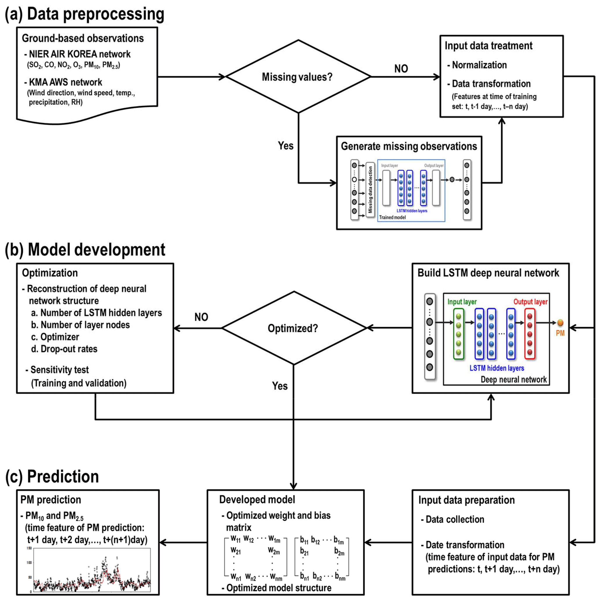
Figure 1Schematic diagram of how the LSTM-based PM10 and PM2.5 prediction system was developed.
However, the accuracy of the 3-D CTM simulations has been reported to be low. Researchers believe that this low accuracy originates from uncertain sources of emission inventory, meteorological fields, initial and boundary conditions, and CTMs themselves (Seaman, 2000; Berge et al., 2001; Liu et al., 2001; Holloway et al., 2008; Tang et al., 2009; Han et al., 2011). Many efforts have been made to enhance the accuracy of the 3-D CTM-based forecasting system. As a part of the efforts, the Korean government decided to develop its own air quality forecasting system mainly based on a new CTM in 2017. This project entailed establishing better bottom-up and top-down emissions, developing improved meteorological fields over East Asia, developing a data assimilation system using satellite-retrieved and ground-based observations, and incorporating new atmospheric chemical and physical processes into the new Korean CTM. Despite all the ongoing efforts, the traditional chemical weather forecasts based on the CTM are still poor at conducting accurate air quality forecasts over South Korea.
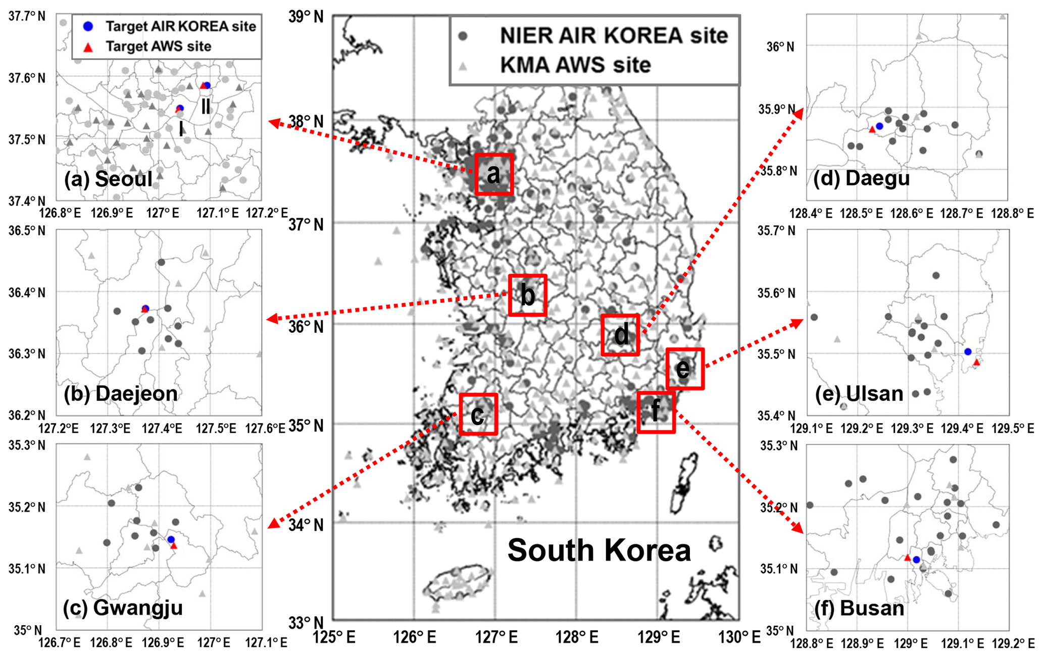
Figure 2Locations of NIER AIR KOREA and KMA AWS sites in South Korea.
In contrast, statistical models based on artificial neural networks (ANNs) have also been applied to air quality predictions. Because these approaches are based on a statistical method instead of sophisticated mathematical model-based computations (i.e., without considerations of advection and convection, photochemistry, or emissions), they are more cost-effective than 3-D CTM simulations. In previous studies, simple ANN models were applied to air quality predictions. The time-series concentrations of ambient pollutants have been predicted by, for example, supported vector machine (SVM) and radial basis function (RBF) neural network models (Lu and Wang, 2005). Furthermore, ambient levels of ozone were predicted by simple feed-forward neural network (FFNN) models (Yi and Rybutok, 1996; Abdul-Wahab and Al-Alawi, 2002). However, such simple models have the limitation of neglecting relationships among data at the different time steps. Recently, more complex ANN models have been developed with recurrent neural networks (RNNs). Although RNNs have typically been used for natural language recognition, they have the special advantage of remembering the experiences of past events because they maintain the activated vectors at each time step (Cho et al., 2014). Because of this advantage, RNNs also make accurate time-series predictions (Che et al., 2018). Several investigators used a shallow (single hidden layer) RNN model to predict the peak mixing ratios of ambient pollutants such as NO2, SO2, O3, CO, and PM10 (Brunelli et al., 2007), and others used a deep RNN model to predict ambient levels of PM2.5 (Ong et al., 2016). However, RNN models have generally shown serious exploding and/or vanishing gradient problems (Bengio et al., 1994; Hochreiter, 1998). To resolve these problems, researchers developed the long short-term memory (LSTM) cell (Hochreiter and Schmidhuber, 1997). Unlike traditional RNNs, LSTM is known to be free from exploding or vanishing gradient problems, and it is better suited for long time-series predictions than are traditional RNNs. Recently, researchers used a deep LSTM neural network to conduct a number of air quality studies (Li et al., 2017; Freeman et al., 2018).
Although ANN-based predictions are not based on mathematics, deep learning has demonstrated a strong potential in the areas of weather and air quality forecasts; for example, the Weather Channel in the United States uses IBM Watson for its operational weather predictions (Mourdoukoutas, 2015). Another example is bias corrections based on several machine-learning techniques. Authors of one study reported that the biases (or errors) between the operational CTM-based air quality predictions and observations can be reduced by utilizing machine-learning algorithms (Reid et al., 2015). There must be many creative ways to improve the accuracy of air quality forecasts by combining 3-D CTM-based predictions with artificial intelligence (AI)-based techniques. These combined approaches have now begun, and this article intends to present one of these efforts in the area of air quality predictions.
For this study, we developed a deep LSTM model to more accurately predict ambient PM concentrations. We evaluated the model performance by comparing the CTM-predicted and observed PM10 and PM2.5 with the LSTM-predicted PM10 and PM2.5. The details of the system development and prediction procedures are presented in Sects. 2 and 3, and limitations of the model are discussed in Sect. 4.
Figure 1 shows the schematic procedures for the deep LSTM-model-based PM predictions. There were two main processes in developing this prediction system: (i) data preprocessing and (ii) structure design and optimization of the deep neural network. It is essential to prepare time-series sequential data sets for both model training and predictions. In this study, we collected ambient pollutant concentrations and meteorological data from ground-based observations. To construct the system, we first screened several AI-based methods including LSTM, such as SVM, relevance vector machine (RVM), and a technique from convolutional neural network (CNN). Based on the results from the screening, we chose a multilayered deep LSTM neural network and conducted iterative model training to optimize the weights and biases of models at seven individual sites. We present the details on developing the system in the following sections.
2.1 Data preprocessing
We collected the observation data from both the NIER AIR KOREA measurement network and the Korea Metrological Administration (KMA) automatic weather station (AWS) network to prepare the input variables. Figure 2 presents the locations of the AIR KOREA and KMA AWS observation sites throughout South Korea; the networks consist of 323 and 494 ground-based monitoring stations, respectively. They provide hourly mixing ratios of the ambient pollutants such as SO2, CO, NO2, O3, PM10, and PM2.5 and the metrological parameters such as temperature, wind direction, wind speed, hourly precipitation, and relative humidity. PM10 and PM2.5 were measured by β-ray absorption and a gravimetric method, respectively (Shin et al., 2011). The ambient mixing ratios of SO2, CO, NO2, and O3 were measured by pulse ultraviolet fluorescence, a nondispersive infrared sensor, chemiluminescence, and ultraviolet methods, respectively.
Among the observation sites, we chose seven monitoring sites located in the major cities in South Korea (Seoul (two sites), Daejeon, Gwangju, Daegu, Ulsan, and Busan) for PM10 and PM2.5 predictions (refer to Fig. 2a–f for the locations). There were two main criteria for selecting the seven sites: (i) the distances between air quality and meteorological monitoring stations should be the shortest (i.e., collocation) and (ii) the number of missing observation data should be minimal. Because there are sometimes too many missing values in the monitoring data prior to 2013, we used observations from January 2014 to April 2016 for training. After the model training, actual predictions of PM10 and PM2.5 were conducted for the period of the Korea-United States Air Quality (KORUS-AQ) campaign (from 1 May to 11 June 2016). The KORUS-AQ campaign period is now an official model testing window in South Korea.
The high quality of input data is critical for LSTM-based time-series predictions. In the current study, the missing values in ground-based air quality monitoring data were produced by using the pretrained deep LSTM model. The percentages of missing observations at the seven AIR KOREA sites are summarized in Table S1 in the Supplement. The percentage ranged between 0.7 % and 13.9 %. The schematic diagram of missing value generation is presented in Fig. S1 in the Supplement. As shown in Fig. S1, when the missing data were detected, the corresponding values were generated from a pretrained model. For example, the accuracy of the missing values generated for the Seoul-1 site is summarized in Fig. S2. It is shown from Fig. S2 that the pollutant concentrations generated by the pretrained model correlated well with the observed concentrations. The correlation coefficients for the model training and validation ranged from 0.60 to 0.91 and from 0.52 to 0.93, respectively. The accuracy of the generated missing values from the seven selected monitoring stations is summarized in Table S2. For the meteorological parameters, we determined the missing variables by interpolating the observed data; in the meteorological data, fewer than 0.01 % of values were missing.
In particular, information on various pollutants is important in the LSTM-based predictions of PM10 and PM2.5. Because H2SO4 and HNO3 are main precursors of inorganic sulfate () and nitrate (), respectively, correct information on the levels of their precursors (SO2 and NO2) is important. Although CO is not directly related to producing particulate matter, we included the mixing ratios in the input data because these are somehow related to the mixing ratios of ozone and hydroxyl radicals (OH).
Meteorological conditions also play an important role in particulate matter concentrations. Both wind direction and speed can represent the origin of air pollutants and intensity of atmospheric turbulence, and precipitation directly affects PM10 and PM2.5 by wet scavenging. In addition, there is a relationship between relative humidity and the levels of hydroxyl radicals because H2O is a main precursor of OH. Water vapor can also influence the amounts of particulate water and nucleation rates in the atmosphere. Therefore, all meteorological parameters measured in the AWS monitoring data set can possibly affect PM concentrations, and thus we used them in the LSTM-based prediction system.
Table 1Summary of model training and validation results.
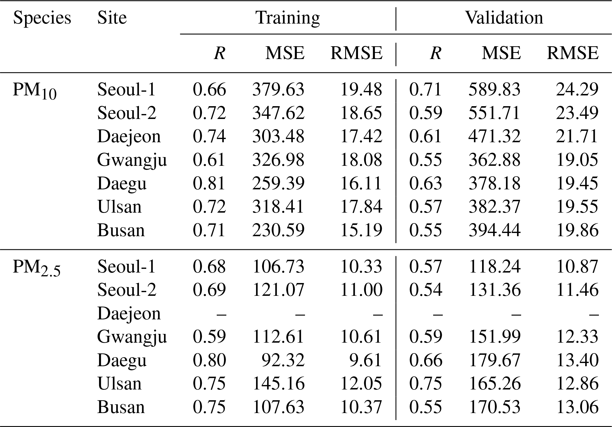
Note: the units for MSE and RMSE are in micrograms per cubic meter (µg m−3).
Before feeding the input variables into the LSTM system, one important step is data normalization. All the input parameters were rescaled between 0 and 1:
where xnormal,i is the normalized values of species i; xi is the observed value; and and are the maximum and minimum values of species i, respectively. Because the LSTM system was designed for daily prediction of PM10 and PM2.5, the normalized observations of the previous day were mapped with the PM concentrations of the next day (i.e., there is a 24 h time lag between independent and dependent variables). Thus, the shapes of one unit of training data are 24×11 and/or 24×12. This structured data set was then re-shaped as a three-dimensional vector matrix to feed them into the hidden LSTM layers. In addition, we excluded the observation data during the dust event periods in the model training; because these episodes are infrequent, including data on them could have interfered with establishing an accurate PM prediction system (i.e., they can be noisy signals).
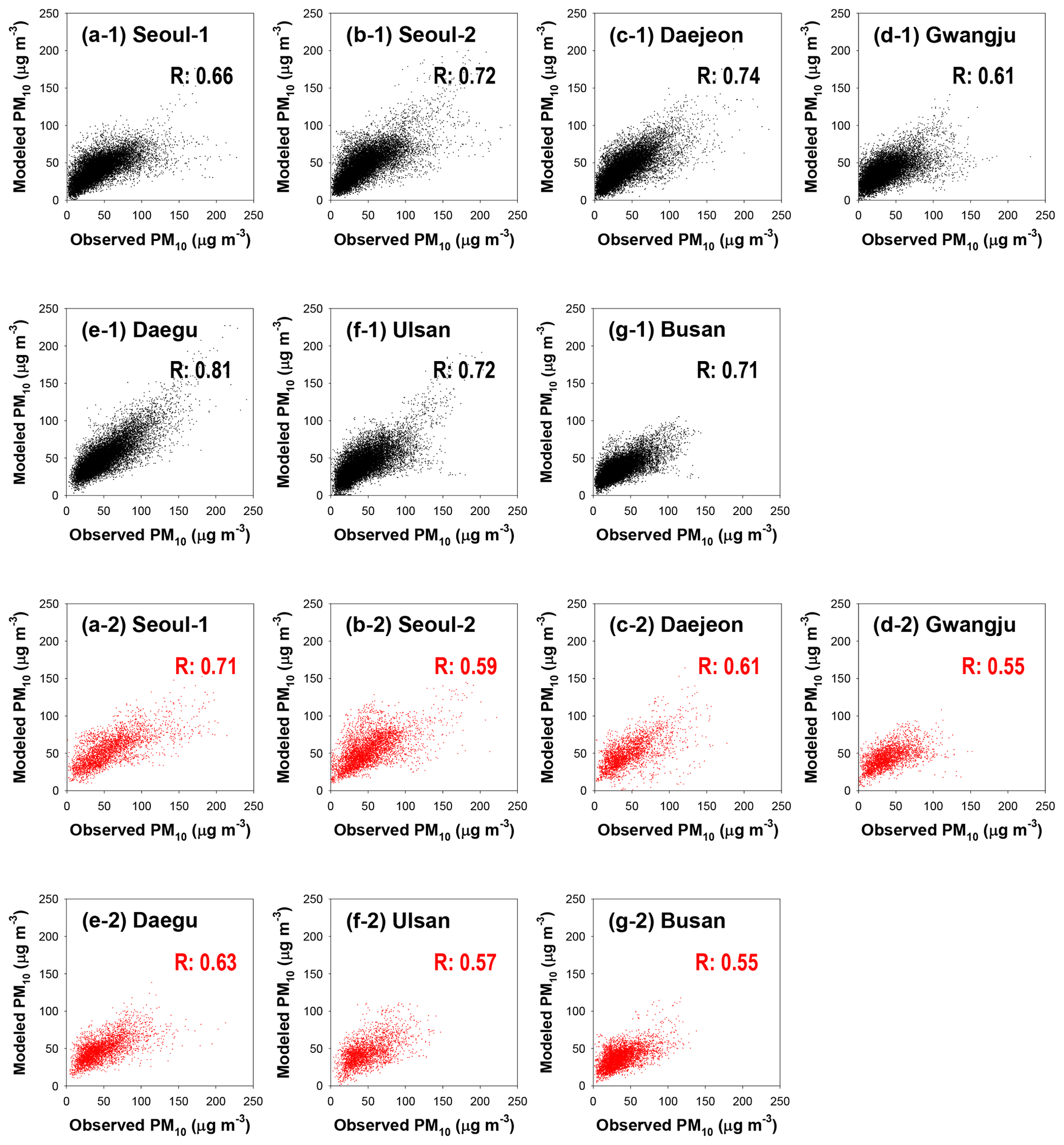
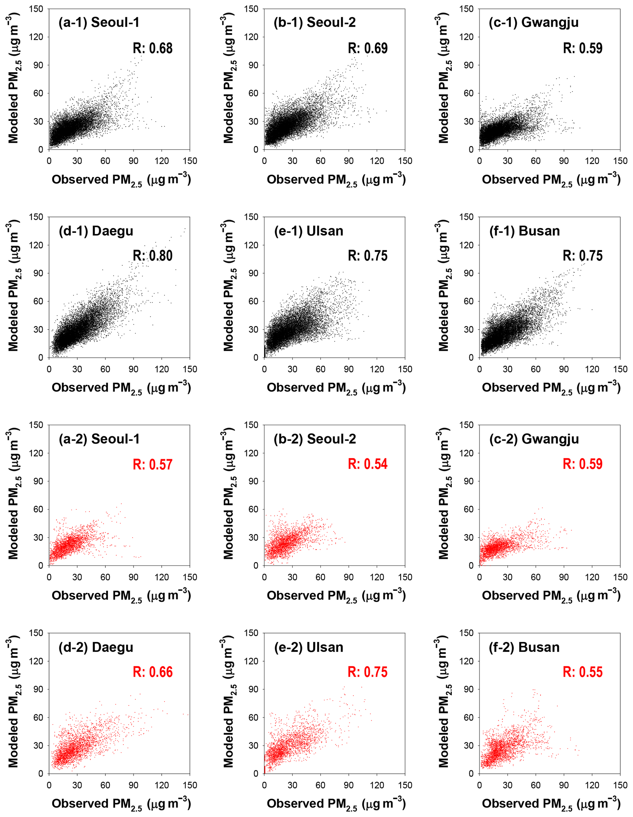
Figure 3Training and validating the daily PM10 prediction model: (a) Seoul-1; (b) Seoul-2; (c) Daejeon; (d) Gwangju; (e) Daegu; (f) Ulsan; (g) Busan. Black and red dots represent the training and validation results, respectively.
2.2 System construction
As mentioned previously, the LSTM has the special advantage of remembering the past experiences. Because of this advantage, the LSTM has a strong capability for identifying highly complex relationship in the sequential data (i.e., the LSTM-based deep neural network has the strong potential in the time-series predictions). In general, the accuracy of the time-series prediction with the deep LSTM model is relatively higher than those with other deep neural networks (Ma et al., 2015; Amarasinghe et al., 2017). Several previous studies have proposed the use of the LSTM for more accurate time-series predictions (e.g., Connor et al., 1994; Saad et al., 1998). Based on this, in this study we used the LSTM cells in the construction of the deep hidden layers of daily PM10 and PM2.5 prediction model.
The developed system has two schemes: PM10 prediction and PM2.5 prediction; the prediction model is designed to have three to five hidden LSTM layers; one layer consists of 100 hidden nodes, and the layers capture sequential temporal information. The last LSTM hidden layer is connected to the output layer, which performs feature mapping between the output vectors from deep hidden layers and the actual PM10 and/or PM2.5.
In order to learn complicated and nonlinear mappings between the layers, activation functions are applied to get the output of a layer, which is then fed into the next layer as an input. There are several activation functions that can be used in neural networks; among them, a sigmoid function has been typically used because it has characteristics of being bounded and being differentiable; however, this function has a vanishing gradient problem due to continuous multiplication of gradients. In this study, therefore, we used the rectified linear unit (ReLU) to activate output layer (Nair and Hinton, 2010). The ReLU is expressed by
As shown in Eq. (2), the ReLU ranges from 0 to ∞. Because the derivative of the ReLU is 0 or 1, the vanishing gradient does not occur during the back propagations. In the Supplement, we give a detailed description of the LSTM architecture used in this study.
In traditional statistics, the close relationship among the input variables (i.e., multicollinearity) can lead to instability of regression coefficients and can distort the effect of the regressive variables on dependent variables. For the deep learning, the multicollinearity requires a relatively long computation time because it is slow to converge. We evaluated the multicollinearity of the independent variables by estimating the Pearson correlation coefficient (R) between the observed atmospheric pollutants at the different time steps because the purpose of recurrent neural network is to identify the relationships in sequential data. The correlation coefficients are summarized in Table S3; as shown in Table S3, there are relatively low correlations among the concentrations of atmospheric pollutants. In addition, the LSTM-based deep neural network is effective for analyzing the relationships between highly correlated time-series sequential data (Fan et al., 2014). Furthermore, the problem of the multicollinearity can be resolved by adopting ReLU as an activation function (Ayinde et al., 2019).
2.3 Model training
The model training is a process for optimizing the structural and learnable parameters of the deep LSTM system; we determined the PM10 and PM2.5 prediction system's structure from the iterative training, and the structure was described in Sect. 2.2. In addition to the activation functions described in Sect. 2.2, there are two more main components in the deep neural network training: (i) cost function and (ii) optimization algorithm. The cost function usually measures how well the neural network works with respect to given training samples and corresponding predicted outputs. In other words, it is used for evaluating the accuracy of predicted values. When the prediction accuracy is poor, the cost is high, whereas as the model's predictions are more accurate, the cost decreases.
There are several cost functions commonly used in deep learning, and the cost function can be classified by its application purpose. In this study, the purpose of the cost function was to minimize the regression cost, and we thus used mean squared error (MSE) as a cost function, expressed as
where xi is the input vector for ith training; yi is the target value (or true value) for the ith training; and hθ(xi) is the predicted vector corresponding to yi for a given deep neural network model θ. It should be noted here that θ means the LSTM network with different parameters (see Eqs. S1–S6 in the Supplement). In Eq. (3), JMSE(θ) represents the MSE between the target vector, yi, and its predicted vector, hθ(xi), when the number of training vectors is N.
The role of an optimization algorithm is to find an efficient and stable pathway for minimizing the gradient descent of a cost function. In this study, we utilized adaptive moment estimation (ADAM) to train the neural networks (Kingma and Ba, 2015). The ADAM is one of the extended algorithms for stochastic gradient descent, and its detailed explanation is also given in the Supplement.
In order to train the LSTM system for the PM10 and PM2.5 predictions, the observations from January 2014 to April 2016 (2.3-year data) were used, as mentioned previously. Because Asian dust is regarded as containing noisy atmospheric signals, we removed the observations during dust events in the course of the model training. We divided the training data set into two groups with ratios of 0.85 to 0.15 for the model training and validation (Guyon, 1997).
First, we measured the variations in training and validation costs (i.e., the outcome of MSE cost) during the model training. In the early stages of the model training, updating the weights and biases decreases the training and validation costs. Because the training data set is only considered for updating weights and biases, the training cost is smaller than the validation cost. With the same reason, the training cost continues to decrease during the model training. In contrast, the validation cost decreases until a certain number of iterations, and then it starts to increase. Optimization of the deep neural network model is to update the weight and bias vectors until the validation cost reaches such an inflection point (Mahsereci et al., 2017). In addition, the model training can also be verified by comparing two statistical parameters, MSE and root mean squared error (RMSE); these values at the inflection point are summarized in Table 1. For properly trained models, the training cost should be slightly smaller than the validation cost. If the validation cost is much higher than training cost and the slope of validation cost is positive, it is called “over-fitting”, which means that both the weight and bias vectors of the model have been overturned. Based on the above two essential requirements of the model training, we concluded that our LSTM PM prediction model was well trained via general rules of the model training (refer to Table 1).
Second, the accuracy of the deep LSTM model training for PM10 and PM2.5 predictions is summarized in Figs. 3 and 4, respectively; in the figures, the black and red dots denote the comparison results between the predicted and observed PM concentrations in the model training and validation, respectively. As shown in Fig. 3, there was reasonable agreement in the PM10 predictions. The R for PM10 training and validation ranged from 0.61 to 0.81 and from 0.55 to 0.71, respectively. The training results for the PM2.5 model also showed reasonable correlations (0.59≤R for training ≤0.80; 0.54≤R for validation ≤0.75).
2.4 3-D CTM simulations
In order to assess the accuracy of the LSTM-based predictions in this study, we compared them with 3-D CTM-based predictions with and without data assimilation (DA). We employed the Community Multiscale Air Quality (CMAQ) model v5.1 for the 3-D CTM simulations. We acquired the metrological fields from Weather Research and Forecasting v3.8.1 model simulations. The domain of the CMAQ model simulations is presented in Fig. 5; the model domain covers northeast Asia with a horizontal resolution of 15 km×15 km and with 27 sigma vertical levels. We used the KORUS v1.0 emission inventory for anthropogenic emissions; this inventory was made for the KORUS-AQ campaign based on three emission inventories: (i) CREATE (Comprehensive Regional Emission inventory for Atmospheric Transport Experiment); (ii) MICS-Asia (Model Inter-Comparison Study for Asia); and (iii) SEAC4RS (Studies of Emissions and Atmospheric Composition, Clouds, and Climate Coupling by Regional Surveys) (Woo et al., 2017). We estimated biogenic emissions from MEGAN v2.1 (Model of Emissions of Gases and Aerosols from Nature) simulations (Guenther et al., 2006). We obtained biomass burning emissions from FINN (Fire INventory from NCAR, http://bai.acom.ucar.edu/Data/fire/, last access: 13 October 2019) (Wiedinmyer et al., 2011). We obtained lateral boundary conditions from the MOZART-4 model simulations (https://www.acom.ucar.edu/wrf-chem/mozart.shtml, last access: 13 October 2019) (Emmons et al., 2010).
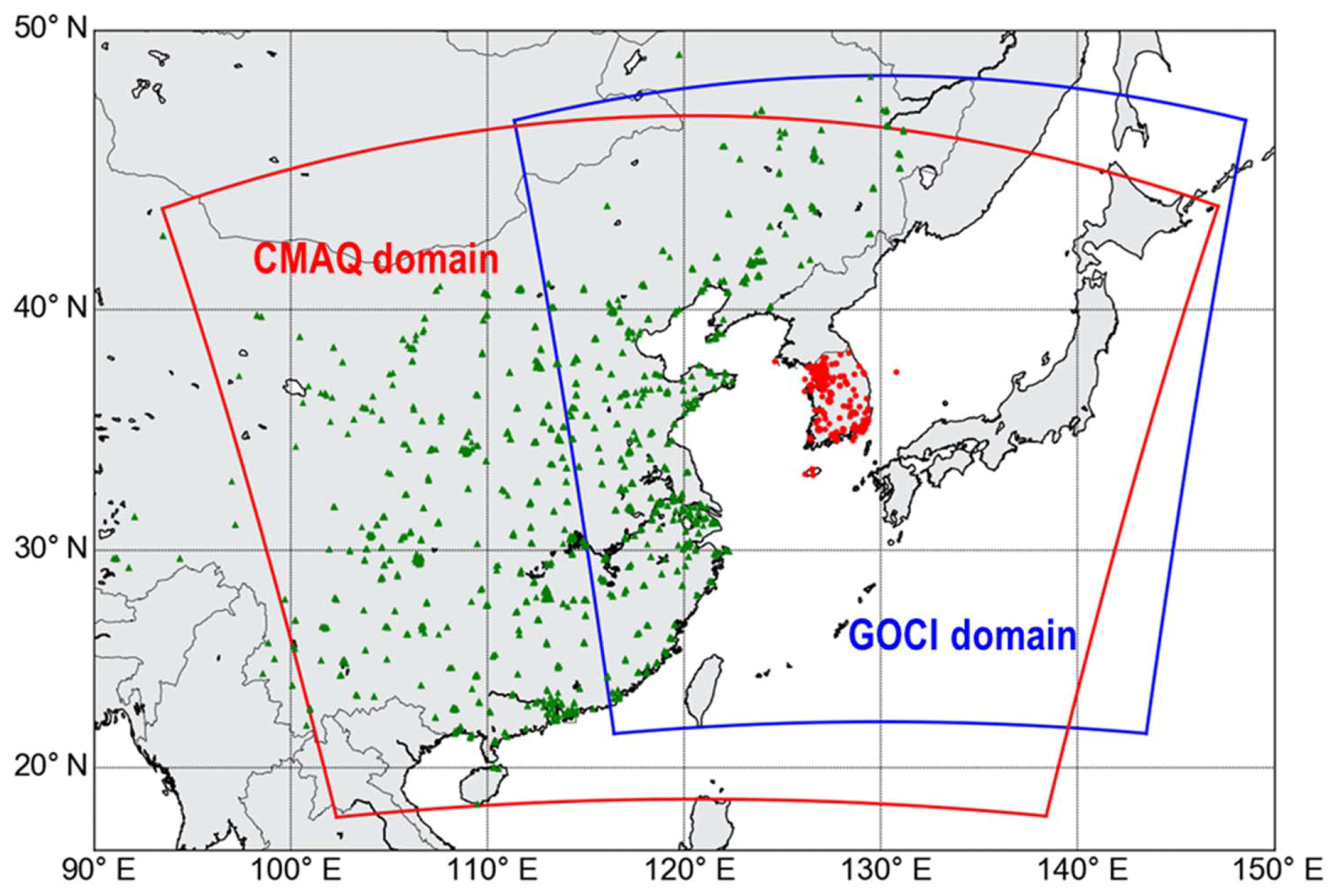
Figure 5Domains of the CMAQ model simulations (red line) and Geostationary Ocean Color Imager (GOCI) sensor (blue line). Green triangles and red dots represent the locations of ground-based monitoring sites in China and South Korea, respectively.
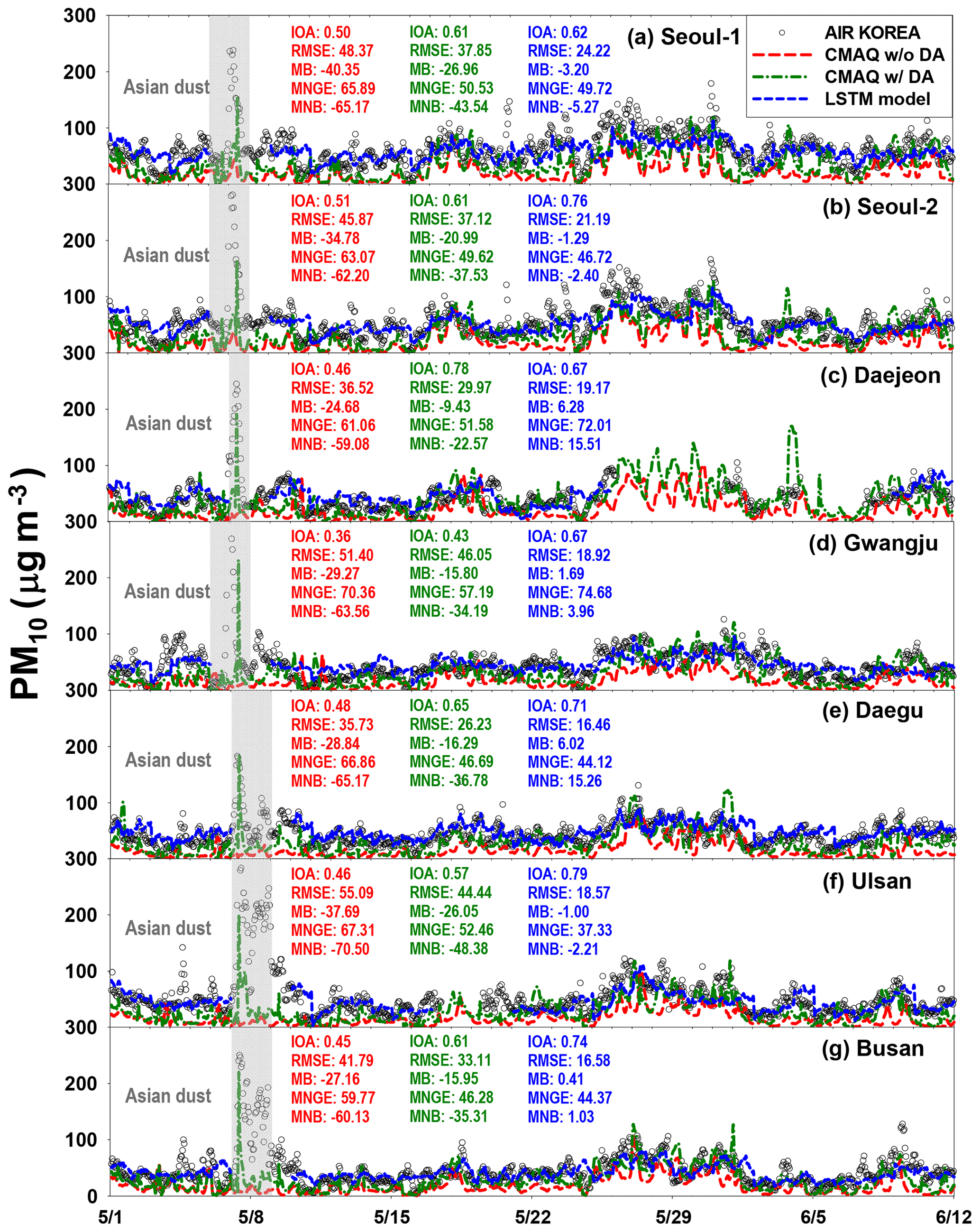
Figure 6Comparisons between the CMAQ-calculated, LSTM-predicted, and the observed PM10. Black open circles show observed PM10 at seven sites. Dashed green and dashed red lines represent CMAQ-predicted PM10 with and without data assimilation, respectively. Dashed blue lines represent LSTM-predicted PM10. From 26 May to 7 June, the LSTM-based PM10 predictions at the Daejeon site were not performed due to the continuous missing observations.
To prepare the initial conditions (ICs) for the CMAQ model simulations, we used the optimal interpolation with Kalman filter method (OI with Kalman). The DA with the OI technique has been used in several previous studies (Carmichael et al., 2009; Chung et al., 2010). The assimilation system is defined as follows:
where τm′ represents the assimilated product; τo and τm denote the observed and modeled values, respectively; H represents the observation and/or forward operator; K represents the Kalman gain matrix; and B and O are the covariance of modeled and observed fields, respectively. B and O can be defined with several free parameters.
where fm, εm, dx, dz, lmx, and lmz represent the fractional error coefficient, minimum error coefficient, horizontal resolution, vertical resolution, horizontal correlation length for errors in modeled values, and vertical correlation length for errors in modeled values, respectively, and fo, εo, and I denote the fractional error coefficient, minimum error coefficient in the observed values, and unit matrix, respectively. The six parameters in Eq. (6) are called the free parameters, which we used to calculate the observation and model error covariance matrix. In this study, we determined these parameters by finding the minimum of χ2:
Here xobs and xassim represent the observed and data-assimilated values, respectively. More detailed explanations regarding the data assimilation can be found elsewhere (Collins et al., 2001; Yu et al., 2003; Park et al., 2011).
For the DA runs, we integrated the CMAQ model simulations with three observation data sets: (i) the Communication, Ocean and Meteorological Satellite (COMS) Geostationary Ocean Color Imager (GOCI) aerosol optical depth (AOD); (ii) ground-based observations in China; and (iii) AIR KOREA observations in South Korea. The locations of the observation stations are presented in Fig. 5. Because the GOCI sensor is geostationary, it can provide hourly spectral images with spatial resolution of 500 m×500 m from 00:00 to 07:00 UTC. Detailed procedures can also be found in previous publications (Park et al., 2014a, b).
PM10 and PM2.5 were predicted for the period of the KORUS-AQ campaign. To evaluate the performance of the LSTM system, we compared the LSTM-based predictions with the observations and two CMAQ-based predictions.
3.1 System evaluation
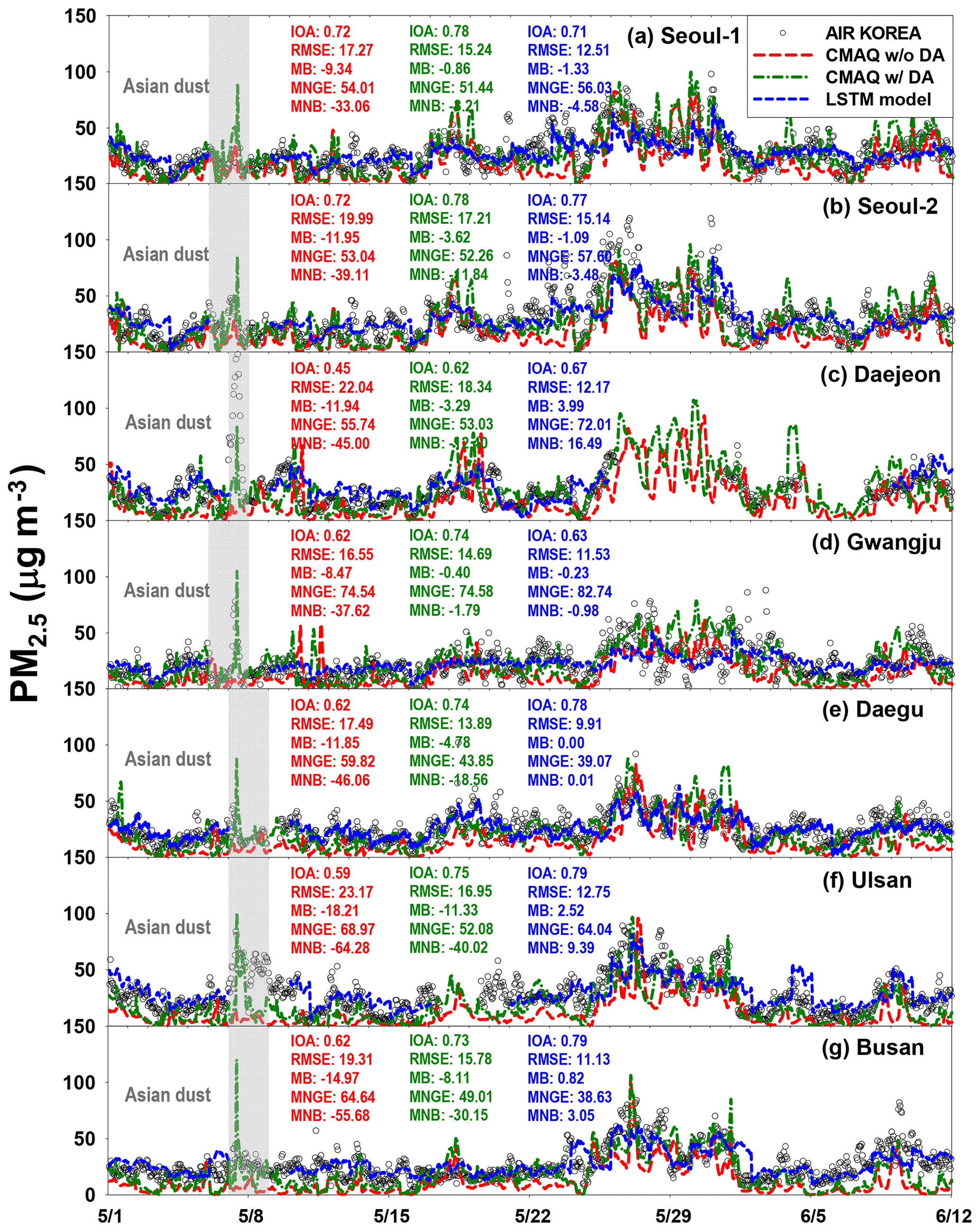
We evaluated the accuracy of the LSTM-based PM predictions by comparing them with the observed PM10 and PM2.5. We also compared PM10 and PM2.5 predicted from two sets of CMAQ model simulations with the PM10 and PM2.5 predicted from the deep LSTM; these results are presented in Figs. 6 and 7. In Figs. 6 and 7, the black circles and dashed blue lines represent the observed and LSTM-predicted PM10 and PM2.5, respectively. The dashed green and dashed red lines denote CMAQ-predicted PM10 and PM2.5 with and without DA, respectively. The CMAQ model simulations with DA showed better agreement with the observations than did those without DA (see Figs. 6 and 7). The LSTM-predicted PM10 also showed good agreement with the observed PM10.
Table 2Statistical analysis with modeled and observed PM10 and PM2.5.
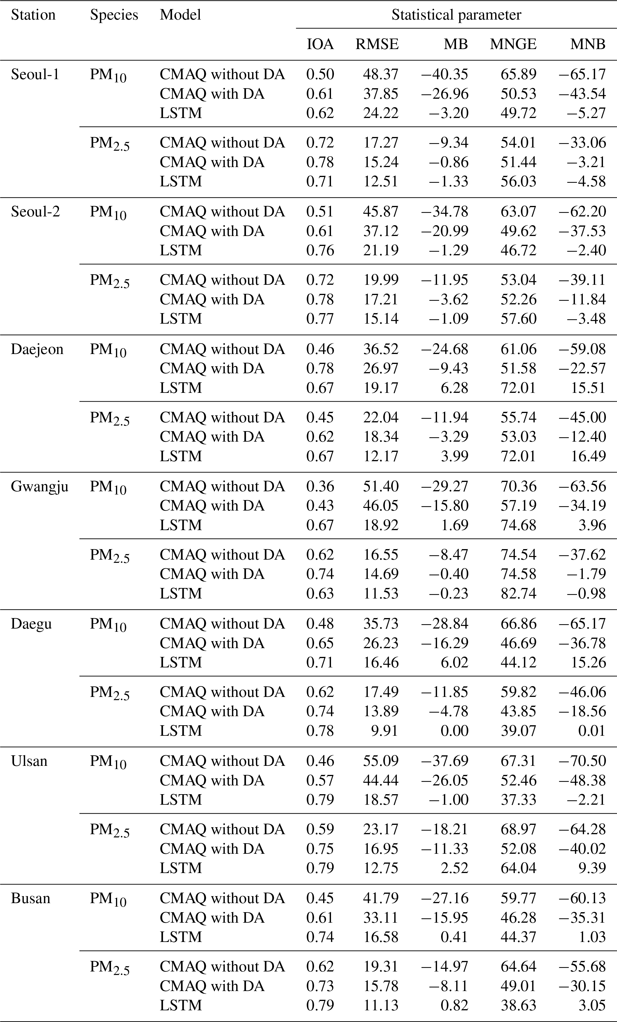
Note: the units for RMSE and MB are micrograms per cubic meter (µg m−3) and those for MNGE and MNB are in percent (%).
However, the results from the CMAQ model simulations were not intended to be directly compared with those from the LSTM predictions. In general, Eulerian CTMs calculate average concentrations of air pollutants in a grid box, but in the real world the concentrations of air pollutants inside a gird box can be (highly) variable with proximity to the local sources (in other words, the air pollutant concentrations in a gird box cannot be uniform). This is well-known problem called “sub-grid variability”. In this sense, both the CMAQ-model results and LSTM predictions were not directly compared. Instead, in this comparison the CMAQ model simulations provide reference values to give a sense of the accuracy of LSTM predictions. One intension to develop the LSTM prediction system is to establish a prediction system at the observation sites (i.e., point site), and we eventually plan to integrate the CTM-LSTM prediction (gird-based prediction and point-based prediction) system for more comprehensive PM forecasting in South Korea. This will be discussed further in Sect. 4.
For further statistical evaluations, we introduced the following five statistical parameters: (i) IOA (index of agreement); (ii) RMSE; (iii) MB (mean bias); (iv) MNGE (mean normalized gross error); and (v) MNB (mean normalized bias).
Here, Ci,Model and Ci,Obs represent the modeled and observed concentrations of species i; is the averaged Ci,Obs. The results from the statistical analysis are summarized in Table 2 and are also shown in Figs. 6 and 7.
For the daily PM10 predictions, the LSTM-based predictions (0.62≤ IOA ≤0.79) were always more accurate than two CMAQ-based PM10 predictions (0.36≤ IOA ≤0.78). RMSE and MB between the CMAQ-based and observed PM10 ranged between 33.11 and 51.40 µg m−3 and between −40.35 and −15.95 µg m−3, respectively. These negative MBs indicate that the CMAQ model simulations underestimated PM10. RMSE and MB between the LSTM-based predictions and observations ranged from 18.57 to 24.23 µg m−3 and from −3.20 to 6.28 µg m−3, respectively. The RMSEs for the LSTM-based predictions are 1.90 times smaller than those for the CMAQ-based predictions. Among the seven sites chosen, the PM10 predictions at the Daegu, Ulsan, and Busan sites showed the best agreement (0.71≤ IOA ≤0.79) and the lowest errors and biases (16.46≤ RMSE ≤18.57; MB ≤6.02) compared with the two CMAQ-based PM10 predictions (0.45≤ IOA ≤0.65; 26.23≤ RMSE ≤55.09; MB ).
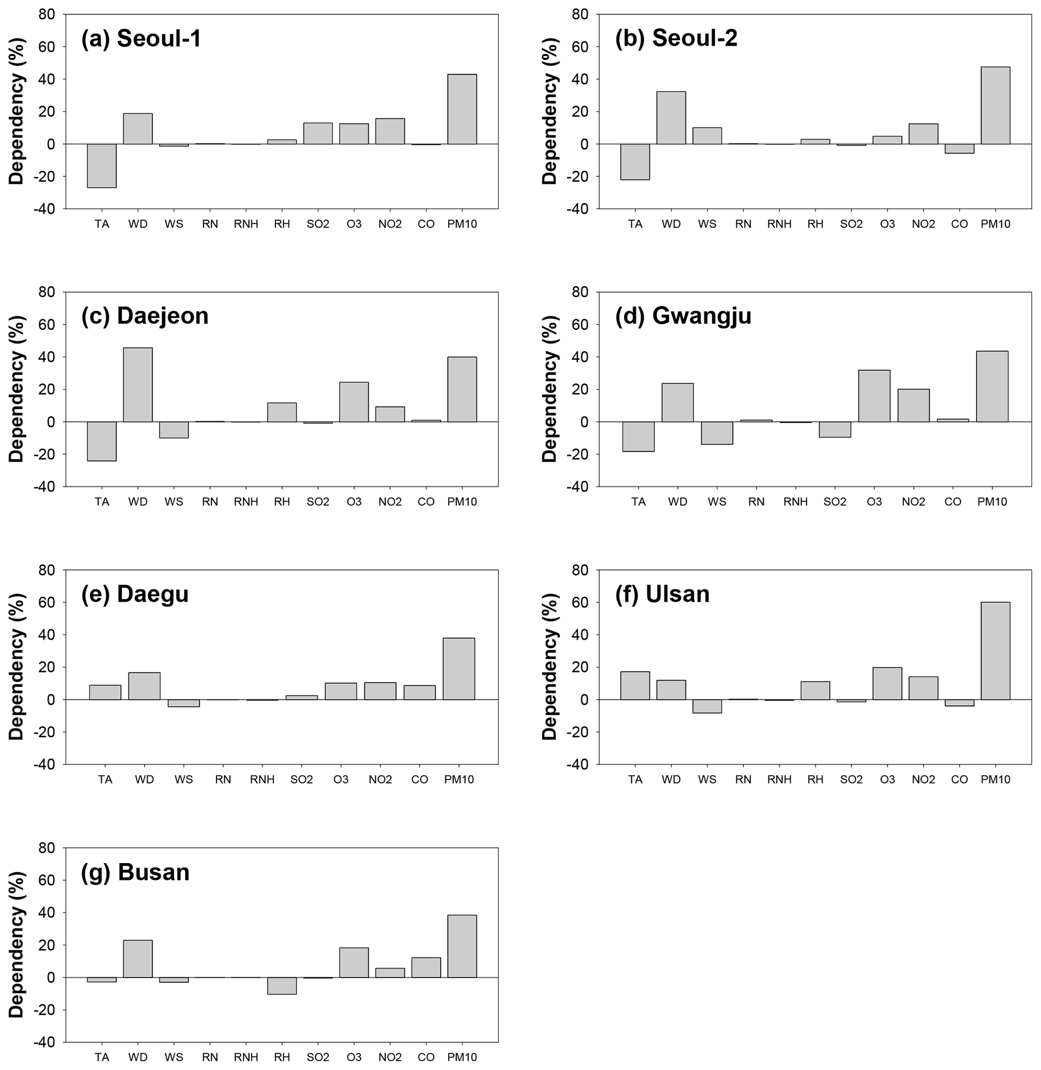
Figure 9Dependencies of input variables on the daily PM10 predictions. TA, WD, WS, RN, RNH, and RH represent temperature, wind direction, wind speed, daily cumulative precipitation, hourly precipitation, and relative humidity, respectively. SO2, O3, NO2, CO, and PM10 refer to the levels of the previous day for these atmospheric pollutants.
Figure 7 presents the comparisons for PM2.5. During the KORUS-AQ campaign, there were no ground PM2.5 observations at the Daejeon site between 1 May and 11 June because of instrument malfunction. The LSTM-predicted PM2.5 again showed good agreement with the observations (0.63≤ IOA ≤0.79); however, the deep LSTM system was not always able to more accurately predict PM2.5. As with PM10, the LSTM PM2.5 predictions at the Daegu, Ulsan, and Busan sites showed better performance (0.78≤ IOA ≤0.79) than the CMAQ-based predictions (0.59≤ IOA ≤0.75), but at the two Seoul sites (Seoul-1 and Seoul-2) the LSTM PM2.5 predictions were inferior to those from the CMAQ model simulations with DA (dashed green lines in Fig. 7). This could have been because the AIR KOREA observation sites are densely located in and around Seoul Metropolitan Area (refer to Fig. 2). Therefore, data assimilation appears to more strongly influence the accuracy of the CMAQ predictions.
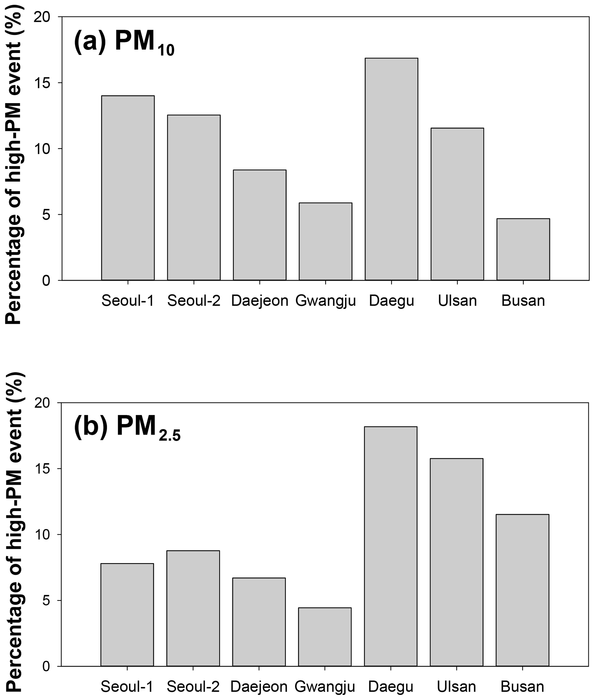
As shown in Figs. 6 and 7, there were nationwide high-PM episodes from 25 to 28 May 2016; these high-PM events were caused by the long-distance transport of atmospheric pollutants from China due to westerlies, and the relatively high errors and biases in the LSTM-based predictions occurred during these high-PM events. Because the model's weights and biases were optimized based on previous memories, frequent high-PM episodes can affect the accuracy of the predictions. The frequencies of the high-PM10 (daily average of PM10 ≥70 µg m−3) and high-PM2.5 (daily average of PM2.5 ≥40 µg m−3) episodes in the training data set are summarized in Fig. 8. The fractions of the high-PM2.5 episodes at the Seoul and Gwangju sites were between 0.04 and 0.09, clearly smaller than those at Daegu, Ulsan, and Busan (0.12≤ high-PM2.5 episode ≤0.18). At Gwangju, the effectiveness of DA and frequency of high-PM episodes were the lowest. As mentioned previously, the LSTM-based PM10 and PM2.5 prediction system was trained using the observation data for only 2.3 years because these were the only available data. The optimized weights and biases are governed by the variety of input features in the training. If more PM2.5 data are available in the future, the prediction accuracy of deep LSTM systems will improve; and in fact, continuous data accumulation with more recent PM data is now underway.
Imbalance of the training data set has deteriorated the performances of the deep neural network model. As shown in Fig. 8, the frequency of high-PM10 and high-PM2.5 events is very low. There are a number of ways to balance the data, such as minority oversampling and majority subsampling. The prerequisite for the data balancing is that the amounts of available data should be very large. As mentioned previously, the AIR KOREA network has monitored ground PM2.5 only since 2015. Therefore, the amount of available data is relatively small, and compulsory data balancing is highly likely to hinder the generalization of the PM prediction model. Therefore, we did not perform the data balancing in this study.
To test the effectiveness of the data balancing, we did balance the data for the observations of the Seoul-1 site; at this site, the CMAQ-based PM2.5 predictions were better than the LSTM-based PM2.5 predictions. Because of the data availability, it was impossible to balance the training data set with the subsampling method, and thus we oversampled atmospheric conditions during the high-PM2.5 events. To balance the numbers of high-PM and non-high-PM events, we replicated the ground observations during the high PM2.5 events; then we generated ±5 % Gaussian random noise on these oversampled data to reflect the observational errors. The PM2.5 predictions with and without the data balancing are represented in Fig. S4. As shown in Fig. S4, the data balancing did not improve the prediction performances of the LSTM model. This is because we could not sample the various types of high-PM2.5 events, and similar patterns of atmospheric conditions were consistently considered in the model training. Therefore, to improve the performances of the LSTM-based PM prediction model, it is necessary to collect various atmospheric conditions through continuous ground-based observations.
3.2 Dependence on input parameters
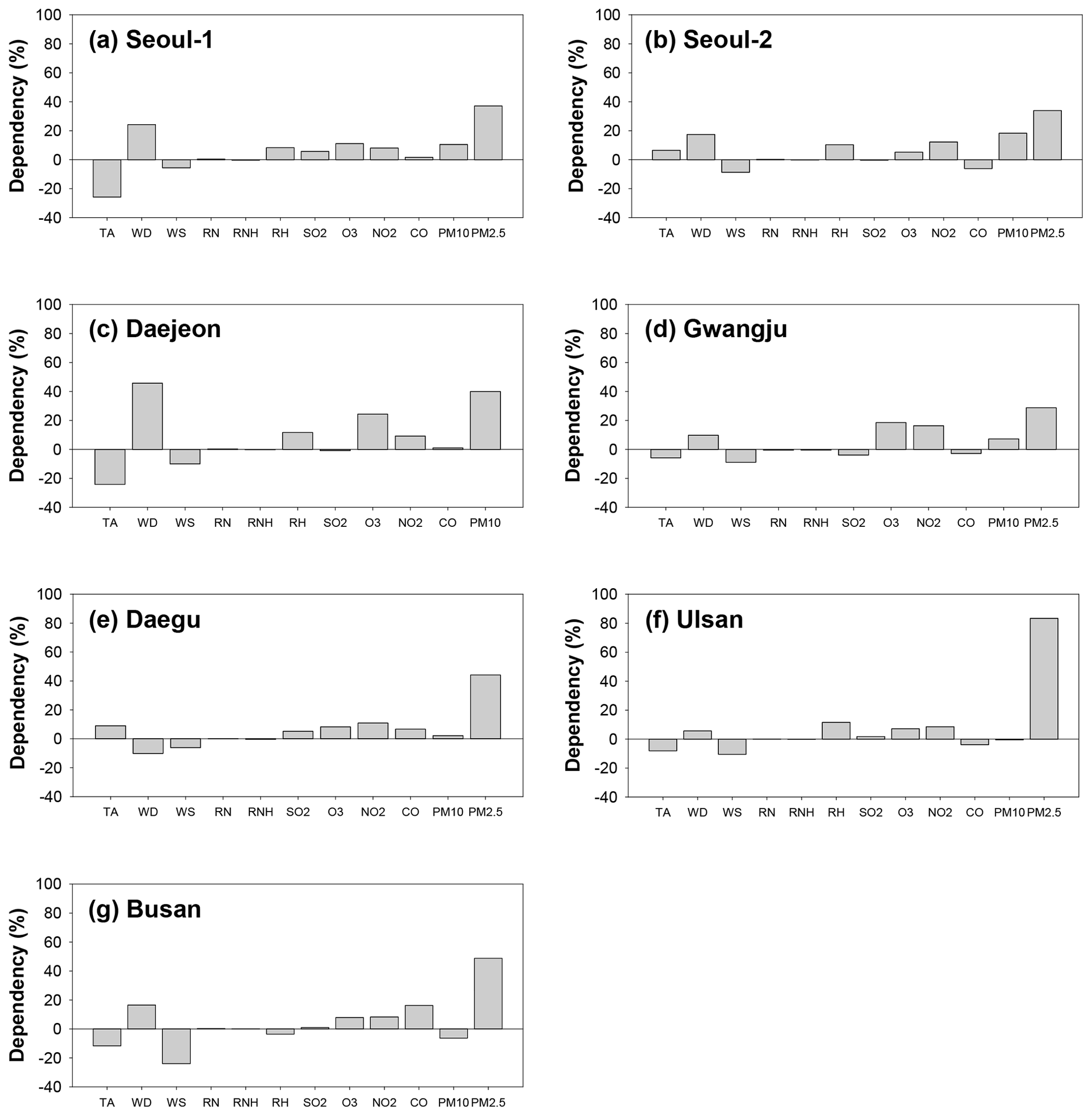
In deep learning, the relationships between input variables and predictions cannot be identified directly because of the high nonlinearity in the hidden layers. In the present study, we indirectly investigated the influences of the input parameters on the PM10 and PM2.5 predictions with and without considering each variable in the model operations. The influences on the input parameters are summarized in Figs. 9 and 10; in the figures, TA, WD, WS, RN, RNH, and RH represent temperature, wind direction, wind speed, daily cumulative precipitation, hourly precipitation, and relative humidity on the previous day, respectively. SO2, O3, NO2, CO, PM10, and PM2.5 are the concentrations of the respective air pollutants on the previous day. The positive and negative values in each figure represent the directionality of the influences on the PM10 and PM2.5 predictions; that is, for instance, the variables with positive dependence indicate increasing influence on the predicted PM10 and PM2.5. The figures show that among the meteorological variables, temperature and wind direction generally had great influence on the PM10 and PM2.5 predictions; among the pollutant variables, previous day PM10 and PM2.5 mainly affected the predictions for the next day. In particular, the dependencies of PM10 and PM2.5 ranged from 38.48 % to 60.12 % and from 28.80 % to 83.38 %, respectively. In most cases, the influence of the pollutant variables (PM10 and PM2.5) was greater than that of the meteorological parameters. However, at Daejeon, the most influential parameter on the PM10 predictions was wind direction (45.67 %), while the contributions of other parameters were relatively small. The difference in the contributions is mainly due to the persistence of each variable. In other words, the variables with low dependence on the PM10 and PM2.5 predictions were those that change rapidly in the atmosphere, and thus their effects are scarcely incorporated into the trained model.
In this study, we established a deep RNN system for daily PM10 and PM2.5 predictions and evaluated the newly developed system's performance by comparing its PM10 and PM2.5 predictions with the observed and CMAQ-predicted levels. In the comparisons, the LSTM-based PM predictions were, in general, superior to the CMAQ-based PM predictions. In terms of IOA, the accuracies of the LSTM predictions were 1.01–1.72 times higher than those for the CMAQ-based predictions. Based on this, we concluded that the LSTM-based system could be applied to daily “operational” PM10 and PM2.5 forecasts. The LSTM-based predictions at the observation sites can provide useful and complementary information for air quality forecasters, synthesizing all the information available such as CTM air quality predictions, AI predictions, weather predictions, and satellite-derived information.
In the future, Korea's air quality forecasting system will be improved by continuous development of the CTM-based prediction system including the use of more advanced DA techniques, together with continuous sophistication of the AI-based prediction system. If the AI-based predictions at the observation sites are consistently better than the CTM-based predictions, the two elements will be more systematically combined within a prognostic mode, which will be our final research goal. In addition, a similar LSTM-based prediction system can also be applied to the daily forecasts of gas-phase air pollutants such as NO2, SO2, CO, and O3. These works are also now in progress.
Although the current LSTM-based system can accurately predict PM10 and PM2.5, it also has some limitations. For better prediction accuracy, we need more air quality data for model optimization. Because PM2.5 has only been monitored in South Korea since 2015, there are too few observations to optimize the PM2.5 predictions, which require continuous accumulation of PM2.5 observations. In addition, the limited number of input variables is another obstacle to optimal model performance. The current LSTM-based PM10 and PM2.5 prediction system contains 10–12 input parameters. If more useful parameters such as mixing layer height (MLH) and barometric distribution are available, its performance would improve further (Hooyberghs et al., 2005; Liu et al., 2007). Therefore, future efforts should be made with more PM2.5 data and more input variables such as mixing layer heights entered into our system.
The source code is available upon personal request to the corresponding author.
The supplement related to this article is available online at: https://doi.org/10.5194/acp-19-12935-2019-supplement.
HSK and IP contributed equally to the paper. HSK and IP led the manuscript writing and contributed to the research design and system development. CHS supervised this study, contributed to the research design and manuscript writing, and served as the corresponding author. KL and KMH contributed to the CMAQ simulations. JWY, HKK, MJ, and JL contributed to the optimization of the deep LSTM model.
The authors declare that they have no conflict of interest.
This work was supported by the National Research Foundation (NRF) of Korea grant funded by the Korean Ministry of Science and ICT (MSIT) (NRF-2016R1C1B1012979) and by the National Strategic Project – Fine particle of the NRF funded by the MSIT, the Ministry of Environment (ME), and the Ministry of Health and Welfare (MOHW) (NRF-2017M3D8A1092022). We obtained NIER AIR KOREA and KMA AWS monitoring data from the official data archives at https://www.airkorea.or.kr/ (last access: 13 October 2019) and https://data.kma.go.kr/ (last access: 13 October 2019), respectively.
This work was supported by NRF of Korea grant funded by the Korean MSIT (NRF-2016R1C1B1012979) and by the National Strategic Project – Fine particle of the NRF funded by the MSIT, the ME, and the MOHW (NRF-2017M3D8A1092022).
This paper was edited by David Topping and reviewed by two anonymous referees.
Abdul-Wahab, S. A. and Al-Alawi, S. M.: Assessment and prediction of tropospheric ozone concentration levels using artificial neural networks, Environ. Modell. Softw., 17, 219–228, 2002.
Amarasinghe, K., Marino, D. L., and Manic, M: Deep neural networks for energy load forecasting, Proceedings of the 26th IEEE International Symposium on Industrial Electronics, 19–21 June, Scotland, UK, 1483–1488, 2017.
Ayinde, B. O., Inanc, T., and Zurada, J. M.: On Correlation of Features Extracted by Deep Neural Networks, arXiv:1901.10900v1, 2019.
Bengio, Y., Simard, P., and Frasconi, P.: Learning long-term dependencies with gradient descent is difficult, IEEE Trans. Neural Networ., 5, 157–166, 1994.
Berge, E., Huang, H.-C., Chang, J., and Liu, T.-H.: A study of importance of initial conditions for photochemical oxidant modeling, J. Geophys. Res.-Atmos., 106, 1347–1363, 2001.
Brunelli, U., Piazza, V., Pignato, L., Sorbello, F., and Vitabile, S.: Two-days ahead prediction of daily maximum concentrations of SO2, O3, PM10, NO2, CO in the urban area of Palermo, Italy, Atmos. Environ., 41, 2967–2995, 2007.
Carmichael, G. R., Adhikary, B., Kulkarni, S., D'Allura, A., Tang, Y., Streets, D., Zhang, Q., Bond, T. C., Ramanathan, V., Jamroensan, A., and Marrapu, P.: Asian aerosols: Current and year 2030 distributions and implications to human health and regional climate change, Environ. Sci. Technol., 43, 5811–5817, 2009.
Che, Z., Purushotham, S., Cho, K., Sontag, D., and Liu, Y.: Recurrent neural networks for multivariate time series with missing values, Sci. Rep., 8, 6085, https://doi.org/10.1038/s41598-018-24271-9, 2018.
Cho, K., van Merrienboer, B., Gulcehre, C., Bougares, F., Schwenk, H., Bahdanau, D., and Bengio, Y.: Learning phrase representations using rnn encoder-decoder for statistical machine translation, Proceedings of the 19th Conference on Empirical Methods in Natural Language Processing, 25–29 October, Doha, Qatar, 1724–1734, 2014.
Chung, C. E., Ramanathan, V., Carmichael, G., Kulkarni, S., Tang, Y., Adhikary, B., Leung, L. R., and Qian, Y.: Anthropogenic aerosol radiative forcing in Asia derived from regional models with atmospheric and aerosol data assimilation, Atmos. Chem. Phys., 10, 6007–6024, https://doi.org/10.5194/acp-10-6007-2010, 2010.
Collins, W. D., Rasch, P. J., Eaton, B. E., Khattatov, B. V., Lamarque, J.-F., and Zender, C. S.: Simulating aerosols using a chemical transport model with assimilation of satellite aerosol retrievals: Methodology for INDOEX, J. Geophys. Res., 106, 7313–7336, 2001.
Connor, J. T., Martin, D., and Atlas, L. E.: Recurrent neural networks and robust time series prediction, IEEE Trans. Neural Networ., 5, 240–253, 1994.
Davidson, C. I., Phalen, R. F., and Solomon, P. A.: Airborne particulate matter and human health: A review, Aerosol Sci. Tech., 39, 737–749, 2005.
Dockery, D. W., Schwartz, J., and Spengler, J. D.: Air pollution and daily mortality: associations with particulates and acid aerosols, Environ. Res., 59, 362–373, 1992.
Emmons, L. K., Walters, S., Hess, P. G., Lamarque, J.-F., Pfister, G. G., Fillmore, D., Granier, C., Guenther, A., Kinnison, D., Laepple, T., Orlando, J., Tie, X., Tyndall, G., Wiedinmyer, C., Baughcum, S. L., and Kloster, S.: Description and evaluation of the Model for Ozone and Related chemical Tracers, version 4 (MOZART-4), Geosci. Model Dev., 3, 43–67, https://doi.org/10.5194/gmd-3-43-2010, 2010.
Fan, Y., Qian, Y., Xie, F.-L., and Soong, F. K.: TTS synthesis with bidirectional LSTM based recurrent neural networks, Proceedings of the 15th Annual Conference of the International Speech Communication Association, 14–18 September, Singapore, Singapore, 1964–1968, 2014.
Forster, P., Ramaswamy, V., Artaxo, P., Berntsen, T., Betts, R., Fahey, D. W., Haywood, J., Lean, J., Lowe, D. C., Myhre, G., Nganga, J., Prinn, R., Raga, G., Schulz, M., and Van Dorland, R.: Changes in atmospheric constituents and in radiative forcing, in: Climate change 2007: The physical science basis. Contribution of working group i to the fourth assessment report of the intergovernmental panel on climate change, edited by: Solomon, S., Qin, D., Manning, M., Chen, Z., Marquis, M., Averyt, K. B., Tignor, M., and Miller, H. L., Cambridge University Press, Cambridge, UK and New York, 2007.
Freeman, B. S., Taylor, G., Gharabaghi, B., and Thé, J.: Forecasting air quality time series using deep learning, J. Air Waste Manage., 68, 866–886, 2018.
Guenther, A., Karl, T., Harley, P., Wiedinmyer, C., Palmer, P. I., and Geron, C.: Estimates of global terrestrial isoprene emissions using MEGAN (Model of Emissions of Gases and Aerosols from Nature), Atmos. Chem. Phys., 6, 3181–3210, https://doi.org/10.5194/acp-6-3181-2006, 2006.
Guyon, I.: A scaling law for the validation-set traning-set size ratio, AT&T Bell Laboratories, https://citeseerx.ist.psu.edu/viewdoc/summary?doi=10.1.1.33.1337 (last access: 16 October 2019), 1997.
Han, K. M., Lee, C. K., Lee, J., Kim, J., and Song, C. H.: A comparison study between model-predicted and OMI-retrieved tropospheric NO2 columns over the Korean peninsula, Atmos. Environ., 45, 2962–2971, 2011.
Hochreiter, S.: The vanishing gradient problem during learning recurrent neural nets and problem solutions, Int. J. Uncertain. Fuzz., 6, 107–116, 1998.
Hochreiter, S. and Schmidhuber, J.: Long short-term memory, Neural Comput., 9, 1735–1780, 1997.
Holloway, T., Spak, S. N., Barker, D., Bretl, M., Moberg, C., Hayhoe, K., Van Dorn, J., and Wuebbles, D.: Change in ozone air pollution over Chicago associated with global climate change, J. Geophys. Res.-Atmos., 113 D22306, https://doi.org/10.1029/2007JD009775, 2008.
Hooyberghs, J., Mensink, C., Dumont, G., Fierens, F., and Brasseur, O.: A neural network forecast for daily average PM10 concentrations in Belgium, Atmos. Environ., 39, 3279–3289, 2005.
Hope III, C. A. and Dockery, D. W.: Health effects of fine particulate air pollution: lines that connect, J. Air Waste Manage., 56, 709–742, 2006.
Kingma, D. and Ba, J.: Adam: A method for stochastic optimization, Proceedings of the 3rd International Conference on Learning Representations, 3–8 May, San Diego, USA, arXiv:1412.6980v9, 2015.
Li, X., Peng, L., Yao, X., Cui, S., Hu, Y., You, C., and Chi, T.: Long short-term memory neural network for air pollutant concentration predictions: Method development and evaluation, Environ. Pollut., 231, 997–1004, 2017.
Liu, T.-H., Jeng, F.-T., Huang, H.-C., Berger, E., and Chang, J. S.: Influences of initial condition and boundary conditions on regional and urban scale Eulerian air quality transport model simulations, Chemosphere-Global Change Science, 3, 175–183, 2001.
Liu, Y., Franklin, M., Kahn, R., and Koutrakis, P.: Using aerosol optical thickness to predict ground-level PM2.5 concentrations in the St. Louis area: A comparison between MISR and MODIS, Remote Sens. Environ., 107, 33–44, 2007.
Lu, W.-Z. and Wang, W.-J.: Potential assessment of the “support vector machine” method in forecasting ambient air pollutant trends, Chemosphere, 59, 693–701, 2005.
Ma, X., Tao, Z., Wang, Y., Yu, H., and Wang, Y.: Long short-term memory neural network for traffic speed prediction using remote microwave sensor data, Transport Res. C Emer., 54, 187–197, 2015.
Mahsereci, M., Ballers, L., Lassner, C., and Henning, P.: Early stopping without a validation set, arXiv:1703.09580, 2017.
Mourdoukoutas, P.: IBM To Buy The Weather Company, Forbes, available at: https://www.forbes.com/ (last access: 13 October 2019), 2015.
Nair, V. and Hinton, G. E.: Rectified linear units improve restricted Boltzmann machines, Proceedings of the 27th International Conference on Machine Learning, 21–24 June, Haifa, Israel, 432, 2010.
Ong, B. T., Sugiura, K., and Zettsu, K.: Dynamically pre-trained deep recurrent neural networks using environmental monitoring data for predicting PM2.5, Neural Comput. Appl., 26, 1553–1566, 2016.
Park, R. S., Song, C. H., Han, K. M., Park, M. E., Lee, S.-S., Kim, S.-B., and Shimizu, A.: A study on the aerosol optical properties over East Asia using a combination of CMAQ-simulated aerosol optical properties and remote-sensing data via a data assimilation technique, Atmos. Chem. Phys., 11, 12275–12296, https://doi.org/10.5194/acp-11-12275-2011, 2011.
Park, R. S., Lee, S., Shin, S.-K., and Song, C. H.: Contribution of ammonium nitrate to aerosol optical depth and direct radiative forcing by aerosols over East Asia, Atmos. Chem. Phys., 14, 2185–2201, https://doi.org/10.5194/acp-14-2185-2014, 2014a.
Park, M. E., Song, C. H., Park, R. S., Lee, J., Kim, J., Lee, S., Woo, J.-H., Carmichael, G. R., Eck, T. F., Holben, B. N., Lee, S.-S., Song, C. K., and Hong, Y. D.: New approach to monitor transboundary particulate pollution over Northeast Asia, Atmos. Chem. Phys., 14, 659–674, https://doi.org/10.5194/acp-14-659-2014, 2014b.
Reid, C. E., Jerrett, M., Petersen, M. L., Pfister, G. G., Morefield, P. E., Tager, I. B., Raffuse, S. M., and Balmes, J. R.: Spatiotemporal prediction of fine particulate matter during the 2008 Northern California wildfires using machine learning, Environ. Sci. Technol., 49, 3887–3896, 2015.
Saad, E. W., Prokhorov, D. V., and Wunsch, D. C.: Comparative study of stock trend prediction using time delay, recurrent and probabilistic neural networks, IEEE Trans. Neural Networ., 9, 1456–1470, 1998.
Seaman, N. L.: Meteorological modeling for air-quality assessments, Atmos. Environ., 34, 2231–2259, 2000.
Shin, S. E., Jung, C. H., and Kim, Y. P.: Analysis of the measurement difference for the PM10 concentrations between Beta-ray absorption and gravimetric methods at Gosan, Aerosol Air Qual. Res., 11, 846–853, 2011.
Tang, Y., Lee, P., Tsidulko, M., Huang, H.-C., McQueen, J. T., DiMego, G. J., Emmons, L. K., Pierce, R. B., Thompson, A. M., Lin, H.-M., Kang, D., Tong, D., Yu, S., Mathur, R., Pleim, J. E., Otte, T. L., Pouliot, G., Young, J. O., Schere, K. L., Davidson, P. M., and Stajner, I.: The impact of chemical lateral boundary conditions on CMAQ predictions of tropospheric ozone over the continental United States, Environ. Fluid Mech., 9, 43–58, 2009.
Wang, S. X., Zhao, B., Cai, S. Y., Klimont, Z., Nielsen, C. P., Morikawa, T., Woo, J. H., Kim, Y., Fu, X., Xu, J. Y., Hao, J. M., and He, K. B.: Emission trends and mitigation options for air pollutants in East Asia, Atmos. Chem. Phys., 14, 6571–6603, https://doi.org/10.5194/acp-14-6571-2014, 2014.
Wiedinmyer, C., Akagi, S. K., Yokelson, R. J., Emmons, L. K., Al-Saadi, J. A., Orlando, J. J., and Soja, A. J.: The Fire INventory from NCAR (FINN): a high resolution global model to estimate the emissions from open burning, Geosci. Model Dev., 4, 625–641, https://doi.org/10.5194/gmd-4-625-2011, 2011.
Woo, J.-H., Kim, Y., Park, R., Choi, Y., Simpson, I. J., Emmons, L. K., and Streets, D. G.: Understanding emissions in East Asia – The KORUS 2015 emissions inventory, Proceedings of the American Geophysical Union Fall Meeting, 11–15 December, New Oreleans, USA, A11Q-04, 2017.
Yi, J. and Prybutok, R.: A neural network model forecasting for prediction of daily maximum ozone concentration in an industrialized urban area, Environ. Pollut., 92 , 349–357, 1996.
Yu, H., Dickinson, R. E., Chin, M., Kaufman, Y. J., Holben, B. N., Geogdzhayev, I. V., and Mishchenko, M. I.: Annual cycle of global distributions of aerosol optical depth from integration of MODIS retrievals and GOCART model simulations, J. Geophys. Res., 108, 4128, https://doi.org/10.1029/2002JD002717, 2003.