the Creative Commons Attribution 4.0 License.
the Creative Commons Attribution 4.0 License.
 | 31 Jan 2019
Analyzing the turbulent planetary boundary layer by remote sensing systems: the Doppler wind lidar, aerosol elastic lidar and microwave radiometer
Gregori de Arruda Moreira
Juan Luis Guerrero-Rascado
Jose A. Benavent-Oltra
Pablo Ortiz-Amezcua
Roberto Román
Andrés E. Bedoya-Velásquez
Juan Antonio Bravo-Aranda
Francisco Jose Olmo Reyes
Eduardo Landulfo
Lucas Alados-Arboledas
The planetary boundary layer (PBL) is the lowermost region of troposphere and is endowed with turbulent characteristics, which can have mechanical and/or thermodynamic origins. This behavior gives this layer great importance, mainly in studies about pollutant dispersion and weather forecasting. However, the instruments usually applied in studies of turbulence in the PBL have limitations in spatial resolution (anemometer towers) or temporal resolution (instrumentation aboard an aircraft). Ground-based remote sensing, both active and passive, offers an alternative for studying the PBL. In this study we show the capabilities of combining different remote sensing systems (microwave radiometer – MWR, Doppler lidar – DL – and elastic lidar – EL) for retrieving a detailed picture on the PBL turbulent features. The statistical moments of the high frequency distributions of the vertical wind velocity, derived from DL, and of the backscattered coefficient, derived from EL, are corrected by two methodologies, namely first lag correction and law correction. The corrected profiles, obtained from DL data, present small differences when compared with the uncorrected profiles, showing the low influence of noise and the viability of the proposed methodology. Concerning EL, in addition to analyzing the influence of noise, we explore the use of different wavelengths that usually include EL systems operated in extended networks, like the European Aerosol Research Lidar Network (EARLINET), Latin American Lidar Network (LALINET), NASA Micro-Pulse Lidar Network (MPLNET) or Skyradiometer Network (SKYNET). In this way we want to show the feasibility of extending the capability of existing monitoring networks without strong investments or changes in their measurements protocols. Two case studies were analyzed in detail, one corresponding to a well-defined PBL and another corresponding to a situation with presence of a Saharan dust lofted aerosol layer and clouds. In both cases we discuss results provided by the different instruments showing their complementarity and the precautions to be applied in the data interpretation. Our study shows that the use of EL at 532 nm requires a careful correction of the signal using the first lag time correction in order to get reliable turbulence information on the PBL.
- Article
(13847 KB) -
Supplement
(880 KB) - BibTeX
- EndNote


The planetary boundary layer (PBL) is the atmospheric layer directly influenced by the Earth's surface that responds to its changes within timescales of around an hour (Stull, 1988). This layer is located at the lowermost region of troposphere and is mainly characterized by turbulent processes and a daily evolution cycle. In an ideal situation, some moments after sunrise, the ground surface temperature increases due to the positive net radiative flux (Rn). This process intensifies the convection, where there is an ascension of warm air masses, causing the downward displacement of colder air masses and consequently causing the convective boundary layer (CBL) or mixing layer (ML). This layer has this name due to the mixing process generated by the ascending air parcels. Slightly before sunset, the gradual reduction of incoming solar irradiance at the Earth's surface causes the decrease of the positive Rn and, consequently, its sign change. In this situation, there is a reduction of the convective processes and a weakening of the turbulence. In this process the CBL leads to the development of two layers, namely a stably stratified boundary layer called the stable boundary layer (SBL) close to the surface and the residual layer (RL) that contains features from the previous day's ML and is just above the SBL.
Knowledge of the turbulent processes in the CBL is important in diverse studies, mainly for atmospheric modeling and pollutant dispersion, since turbulent mixing can be considered the primary process by which aerosol particles and other scalars are transported vertically in the atmosphere. Because turbulent processes are treated as nondeterministic, they are characterized and described by their statistical properties (high-order statistical moments). When applied to atmospheric studies, such an analysis provides information about the field of turbulent fluctuation as well as a description of the mixing process in the PBL (Pal et al., 2010).
Anemometer towers have been widely applied in studies about turbulence (e.g., Kaimal and Gaynor, 1983; van Ulden and Wieringa, 1996), however the limited vertical range of this equipment restricts the analysis to regions close to surface. Aircrafts have also been used in atmospheric turbulence studies (e.g., Lenschow et al., 1980, 1994; Williams and Hacker, 1992; Albrecht et al., 1995; Stull et al., 1997; Andrews et al., 2004; Vogelmann et al., 2012), nevertheless their short time window limits the analysis. In this scenario, systems with high spatial and temporal resolution and an adequate range are necessary in order to provide more detailed results along the day throughout the whole thickness of the PBL.
In the last decades, lidar systems have been increasingly applied in this kind of study due to their large vertical range; high data acquisition rate; and capability to detect several observed quantities such as vertical wind velocity (Doppler lidar; e.g., Lenschow et al., 2000; Lothon et al., 2006; O'Connor et al., 2010), water vapor (Raman lidar and differential absorption lidar – DIAL; e.g., Wulfmeyer, 1999; Kiemle et al., 2007; Wulfmeyer et al., 2010; Turner et al., 2014; Muppa et al., 2016), temperature (rotational Raman lidar; e.g., Behrendt et al., 2015) and aerosol (elastic lidar; e.g., Pal et al., 2010; McNicholas and Turner, 2014). This allows for the observation of a wide range of atmospheric processes. For example, Pal et al. (2010) demonstrated how the statistical analyses obtained from high-order moments of elastic lidar can provide information about aerosol plume dynamics in the PBL region. In addition, when different lidar systems operate synergistically, as in Engelmann et al. (2008), for example, who combined elastic and Doppler lidar data, it is possible to identify very complex variables such as vertical particle flux.
Different works (Ansmann et al., 2010; O'Connor et al., 2010) have evidenced the feasibility of characterizing the PBL turbulence by DL. Pal et al. (2010) have shown the feasibility of retrieving information on the PBL turbulence from high-order moments of elastic lidar operating at 1064 nm. These approaches are even more attractive when considering facilities of networks, e.g., the European Aerosol Research Lidar Network (EARLINET; Pappalardo et al., 2014), microwave radiometer network (MWRNET; Rose et al., 2005; Caumont et al., 2016) and European Research Infrastructure for the observation of Aerosol, Clouds and Trace gases (ACTRIS) CLOUDNET (Illingworth et al., 2007). For these reasons, and keeping in mind the wide spread of elastic lidar systems operated at other wavelengths like 532 or 355 nm, it would be a worthy test of the feasibility of these other wavelengths in the characterization of the turbulent PBL behavior.
The use of simple techniques, applied to the aforementioned remote systems, provides robust and similar information on the PBL height (PBLH) during the convective period (see, for example, Moreira et al., 2018) or complementary information when the CBL is substituted by the presence of the SBL and the RL (Moreira et al., 2019). Thus, the combination of information obtained from the active remote sensing systems, Doppler lidar (DL) and elastic lidar (EL), acquired with a temporal resolution close to 1 s, and that provided by the microwave radiometer (MWR) can provide a detailed understanding about different features of the PBL, like its structure (CBL versus SBL and RL), the height of the layers, and the rate of growth of the PBLH and turbulence.
In this study we show the feasibility of obtaining clear insight into the PBL behavior using a combination of active and passive remote sensing systems (EL, DL and MWR) acquired during the Sierra Nevada Lidar AerOsol Profiling Experiment (SLOPE-I) campaign, held at IISTA-CEAMA (Andalusian Institute for Earth System Research, Granada, Spain) from May to August 2016. One of the goals is to show the feasibility of using EL at 532 nm, considering the widespread use of lidar systems based on laser emission at this wavelength in different coordinated networks, like EARLINET (Pappalardo et al., 2014) and LALINET (Latin American Lidar Network; Guerrero-Rascado et al., 2016). In addition, this study shows the variety of applications that can be done with EARLINET data, applying some simple changes to the data acquisition procedures.
This paper is organized as follows. Descriptions of the experimental site and the equipment setup are presented in Sect. 2. The methodologies applied are introduced in Sect. 3. Section 4 presents the results of the analyses using the different methodologies. Finally, conclusions are summarized in Sect. 5.
The SLOPE-I campaign was performed from May to September 2016 in southeastern Spain in the framework of the ACTRIS. The main objective of this campaign was to perform a closure study by comparing remote sensing system retrievals of atmospheric aerosol properties, using remote systems operating at the IISTA-CEAMA and in situ measurements operating at different altitudes in the northern slope of the Sierra Nevada, around 20 km away from IISTA-CEAMA (Bedoya-Velásquez et al., 2018; Román et al., 2018). The IISTA-CEAMA station is part of the EARLINET (Pappalardo et al., 2014) since 2005 and, at present, is an ACTRIS station (https://www.actris.eu/DataServices/ObservationalFacilities/AccesstoObservationalFacilities.aspx, last access: 21 January 2019). The research facilities are located at Granada, a medium-sized city in southeastern Spain (Granada; 37.16∘ N, 3.61∘ W; 680 m a.s.l.), surrounded by mountains and with Mediterranean continental climate conditions that are responsible for cool winters and hot summers. Rain is scarce, especially from late spring to early autumn. Granada is affected by a different kind of aerosol particles the originated locally and is affected by medium–long-range particles transported from Europe, Africa and North America (Lyamani et al., 2006; Guerrero-Rascado et al., 2008, 2009; Titos et al., 2012; Navas-Guzmán et al., 2013; Valenzuela et al., 2014; Ortiz-Amezcua et al., 2014, 2017).
MULHACÉN is a biaxial ground-based Raman lidar system operated at IISTA-CEAMA in the frame of the EARLINET. This system operates with a pulsed Nd:YAG laser, with its frequency doubled and tripled by potassium dideuterium phosphate crystals, emitting at wavelengths of 355, 532 and 1064 nm and with output energies per pulse of 60, 65 and 110 mJ, respectively. MULHACÉN operates with three elastic channels, 355, 532 (parallel and perpendicular polarization) and 1064 nm, and three Raman-shifted channels, 387 (from N2), 408 (from H2O) and 607 nm (from N2). MULHACÉN's overlap is complete at 90 % between 520 and 820 m a.g.l. for all the wavelengths, reaching full overlap around 1220 m a.g.l. (Navas-Guzmán et al., 2011; Guerrero-Rascado et al., 2010). Calibration of the depolarization capabilities is done following Bravo-Aranda et al. (2013). This system was operated with a temporal and spatial resolution of 2 s and 7.5 m, respectively. More details can be found in Guerrero-Rascado et al. (2008, 2009).
The Doppler lidar (Halo Photonics, model Stream Line XR) is also operated at IISTA-CEAMA. Since May 2016, this system works in a continuous and automatic mode. It operates at 1.5 µm, with pulse energy and repetition rate of 100 µJ and 15 KHz, respectively. This system records the backscattered signal with a range resolution of 30 m in 300 range gates, with the first range gate starting at 60 m from the instrument. The telescope focus is set to approximately 800 m. The instrument was operated in vertical stare mode with a temporal resolution of 2 s.
Furthermore, we operated the ground-based passive microwave radiometer (RPG-HATPRO G2, Radiometer Physics GmbH), which is member of the MWRNET (http://cetemps.aquila.infn.it/mwrnet/, last access: 21 January 2019). Since November 2011, this system operates in an automatic and continuous mode at IISTA-CEAMA. The microwave radiometer (MWR) measures the sky brightness temperature with a radiometric resolution between 0.3 and 0.4 K root-mean-square error at 1 s integration time, using direct detection receivers within two bands: the K band (water vapor; frequencies of 22.24, 23.04, 23.84, 25.44, 26.24, 27.84 and 31.4 GHz) and V band (oxygen; frequencies of 51.26, 52.28, 53.86, 54.94, 56.66, 57.3 and 58.0 GHz). From these bands, it is possible to obtain profiles of water vapor and temperature with the inversion algorithms described in Rose et al. (2005). The range resolution of these profiles vary between 10 and 200 m in the first 2 km and between 200 and 1000 m in the layer between 2 and 10 km (Navas-Guzmán et al., 2014).
The meteorological sensor (HMP60, Vaisala) is used to register the air surface temperature and surface relative humidity with a temporal resolution of 1 min. Relative humidity is monitored with an accuracy of ±3 %, and air surface temperature is acquired with an accuracy and precision of 0.6 and 0.01 ∘C, respectively.
A CM-11 pyranometer manufactured by Kipp & Zonen (Delft, The Netherlands) is also installed in the ground-based station. This equipment measures the shortwave (SW) solar global horizontal irradiance data (305–2800 nm). The CM-11 pyranometer complies with the specifications for the first-class WMO (World Meteorological Organization) classification of this instrument (resolution better than ±5 W m−2), and the calibration factor of stability has been periodically checked against a reference CM-11 pyranometer (Antón et al., 2012).
3.1 MWR data analysis
The MWR data are analyzed combining two algorithms, the parcel method (PM; Holzworth, 1964) and the temperature gradient method (TGM; Coen et al., 2014), in order to estimate the PBL height (PBLHMWR) in convective and stable situations, respectively. The different situations are differentiated by comparing the surface potential temperature (θ(z0)) with the corresponding vertical profile of θ(z) up to 5 km. The cases in which all the points in the vertical profile have values larger than θ(z0) are labeled as stable, and the TGM is applied. Otherwise the situation is labeled as unstable, and the PM is applied. The vertical profile of θ(z) is obtained from the vertical profile of T(z) using the following equation (Stull, 2011):
where T(z) is the temperature profile provided by MWR, z is the height above sea level, and 0.0098 K m−1 is the dry adiabatic temperature gradient. A meteorological station co-located with the MWR is used to detect the surface temperature (T(z0)). In order to reduce the noise, θ(z) profiles were averaged providing a PBLHMWR value at 30 min intervals. This methodology of PBLH detection was selected as the reference due to the results obtained during a performed intercomparison campaign between MWR and radiosonde data, where 23 radiosondes were launched. High correlations were found between PBLH retrievals provided by both instruments in stable and unstable cases. Further details are given by Moreira et al. (2018).
3.2 Lidar retrieval of the PBLH
The simple processing of DL and EL data allows for the estimation of the CBL height. Moreira et al. (2018) have discussed this issue in depth, while Moreira et al. (2019) have used the complementarity of the data obtained from distinct remote sensing systems in order to distinguish the sub-layers during the period when the SBL and RL substitute for the CBL as well as during complex situations, like the presence of dust layers.
The PBLH obtained from DL data (PBLHDoppler) is estimated from the variance threshold method. In this method the PBLHDoppler is attributed to the height where the variance of vertical wind speed () is lower than a determinate threshold, which was adopted as 0.16 m2 s−2 (Moreira et al., 2018). For the PBLHDoppler, calculations were selected from a time interval of 30 min. Concerning the PBLH obtained from EL (PBLHElastic), the variance method is applied. This method assumes the maximum of the variance of range corrected signal () as PBLHElastic (Moreira et al., 2015). The is obtained from a time interval of 30 min.
3.3 Lidar turbulence analysis
Both lidar systems, DL and EL, gathered data (q(z,t)) with a temporal resolution of 2 s. Then, the data are averaged in 1 h packages from which the mean value is extracted (). This mean value is subtracted from each q(z,t) profile in order to estimate the vertical profile of the fluctuation for the measured variable (; i.e., vertical velocity for the DL):
Then, from , it is possible to obtain the high-order moments (variance – σ2, skewness – S – and kurtosis – K) as well as the integral timescale (τ, which is the time over which the turbulent process are highly correlated to itself) as shown in Table 1. These variables can also be obtained from the following autocovariance function, Mij:
where tf is the final time, and i and j indicate the order of autocovariance function.
However, it is necessary to consider that the acquired real data contain instrumental noise, ε(z). Therefore, Eq. (3) can be rewritten as
The autocovariance function of a time series with zero lag results in the sum of the variances of the atmospheric variable and its ε(z). Nevertheless, atmospheric fluctuations are correlated in time, but the ε(z) is random and uncorrelated with the atmospheric signal. Consequently, the noise is only associated with lag 0 (Fig. 1). Based on this concept Lenschow et al. (2000) made the suggestion of obtaining the corrected autocovariance function, M11(→0), from two methods, namely first lag correction or law correction. In the first method, M11(→0) is obtained directly by the subtraction of lag 0, ΔM11(0), from the autocovariance function, M11(0). In the second method, M11(→0) is generated by the extrapolation of M11(0) at the first nonzero lags back to lag zero ( law correction). The extrapolation can be performed using the inertial subrange hypothesis, which is described by the following equation (Monin and Yaglom, 1979):
where C represents a parameter of the turbulent eddy dissipation rate. The high-order moments and τ corrections and errors are shown in Table 1 (columns 2 and 3, respectively).
Table 1Variables applied to statistical analysis (Lenschow et al., 2000).
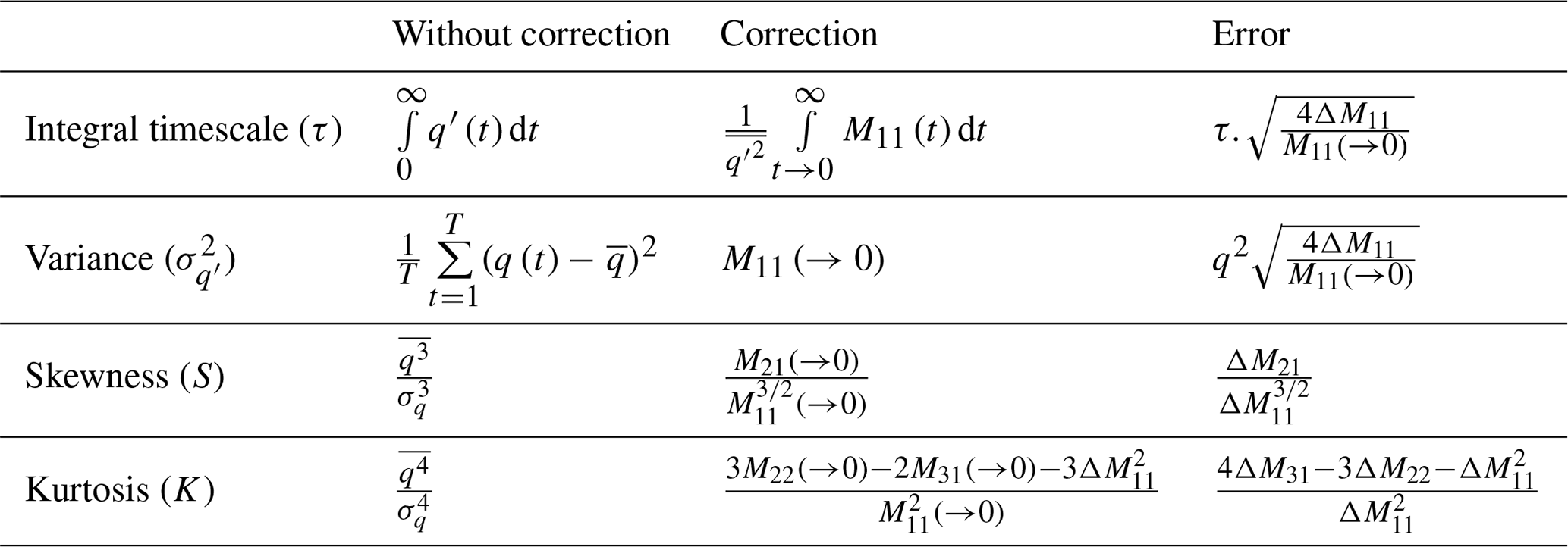
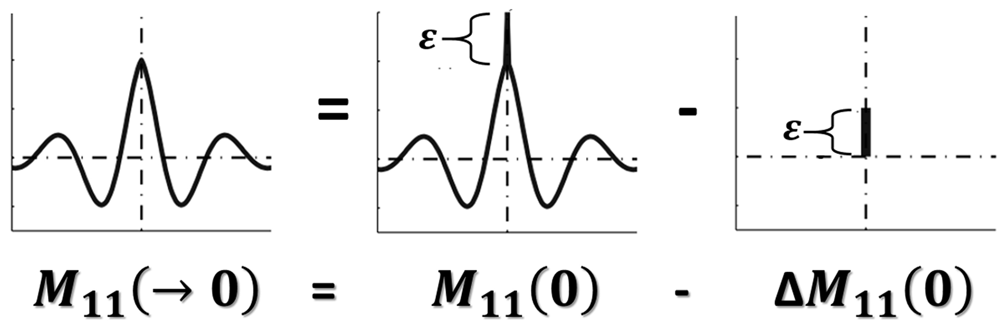
Figure 1Procedure to remove the errors of autocovariance functions. M11(→0) is corrected autocovariance function errors, M11(0) is autocovariance function without correction and ΔM11(0) is error of autocovariance function.
The same procedure of analysis is applied in studies with DL and EL, with the main difference being the tracer used by each system, which is the fluctuation of vertical wind speed (w′) for DL and aerosol number density (N′) for EL. DL provides w(z,t) directly, and therefore the procedure described in Fig. 2 can be directly applied. Thus, the two corrections described above are applied separately, and τ and high-order moments with and without corrections can finally be estimated.
On the other hand, the EL does not provide N(z,t) directly. Under some restrictions, it is possible to ignore the particle hygroscopic growth and to assume that the vertical distribution of aerosol type does not changes with time, therefore adopting the following relation (Pal et al., 2010):
where βpar and represent the particle backscatter coefficient and its fluctuation, respectively, and Y(z) does not depend on time.
Considering the lidar equation,
where Pλ(z) is the signal returned from distance z at time t, z is the distance (m) from the lidar of the volume investigated in the atmosphere, P0 is the power of the emitted laser pulse, c is the light speed (m s−1), td is the duration of laser pulse (ns), A is the area (m2) of telescope cross section, O(z) is the overlap function, αλ(z) is the total extinction coefficient (due to atmospheric particles and molecules; (km)−1) at distance z, βλ(z) is the total backscatter coefficient (due to atmospheric particles and molecules; (km sr)−1) at distance z and the subscript λ represents the wavelength. The two-path transmittance term related to α(z) is considered nearly negligible at 1064 nm (Pal et al., 2010). Thus, it is possible to affirm that
and, consequently, that
where RCS1064 and RCS are the range corrected signal and its fluctuation, respectively, G is a constant, and the subscripts represent the wavelength.
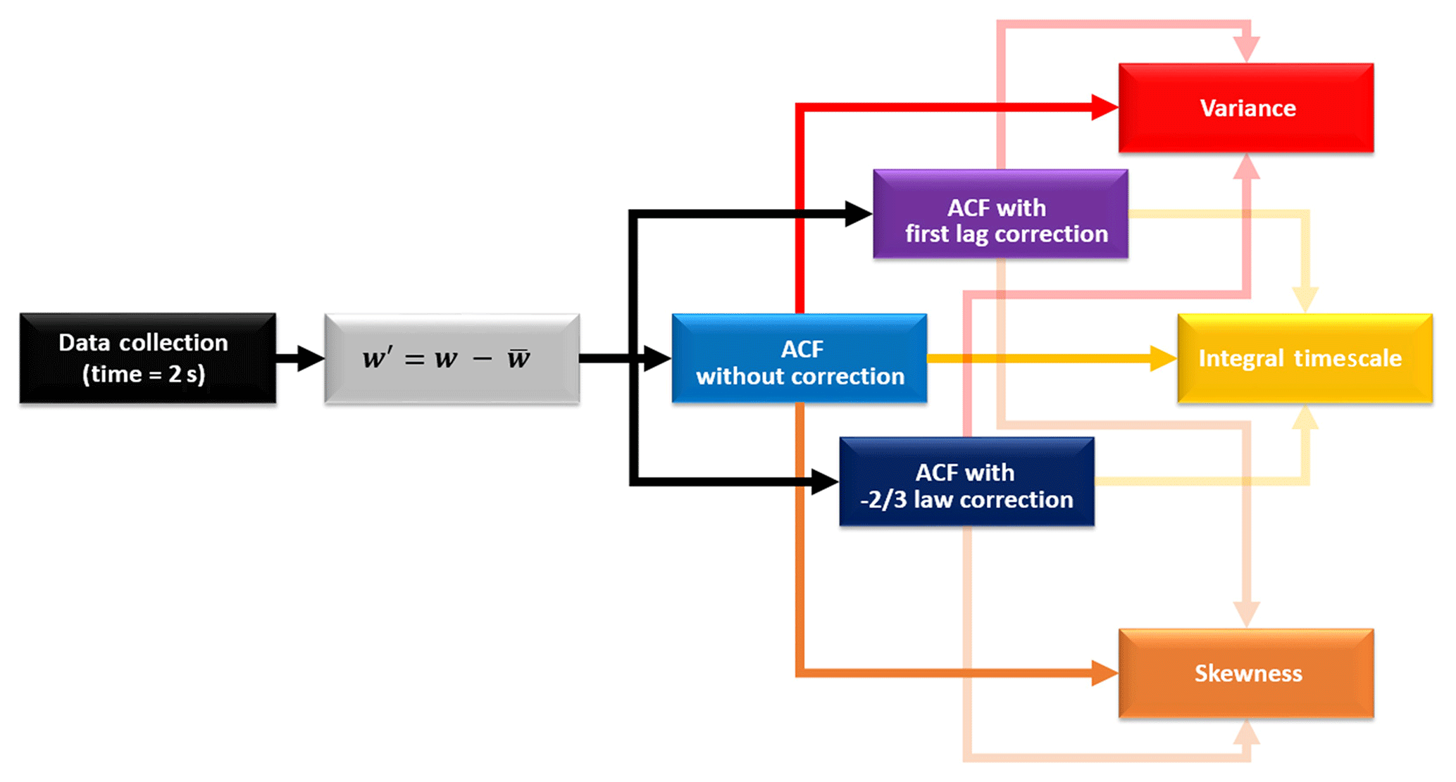
Figure 2Flowchart of data analysis methodology applied to the study of turbulence with Doppler lidar.
In this way, Pal et al. (2010) have shown the feasibility of using EL operating at 1064 nm for describing the atmospheric turbulence. However, keeping in mind the more extended use of lidar systems based on laser emission at 532 nm in different coordinated networks, e.g., in EARLINET and LALINET, around 76 % and 45 % of the systems include the wavelength of 1064 nm, while 95 % of the EARLINET systems and 73 % of the LALINET systems operate systems that include the wavelength 532 nm (Guerrero-Rascado et al., 2016); in this study we use RCS532 fluctuations to determine turbulence, following the procedure described in Fig. 3. This EL methodology is very similar to that described earlier for DL.
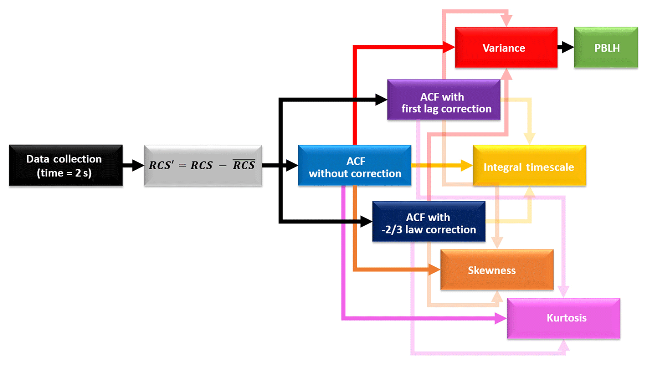
Figure 3Flowchart of data analysis methodology applied to the study of turbulence with elastic lidar.
We perform the validation of the RCS532 in analyses about turbulence using EL, following the procedure described in Fig. 3, which is basically the same methodology described earlier for DL.
4.1 Error analysis
The influence of random error in noisy observations rapidly grows for higher-order moments (i.e., the influence of random noise is much larger for the fourth-order moment than for the third-order moment). Therefore, for the first step, in order to ascertain the applied methodology and our data quality, we performed the error treatment of DL data, as described in Fig. 2. For the DL analysis we selected the period 08:00–09:00 UTC on 19 May, the same day that will be presented in Case Study 1. This day is characterized by a well-defined PBL.
Figure 4 illustrates the autocovariance function, generated from w′, at three different heights. As mentioned before, the lag 0 is contaminated by noise (ε), and thus the impact of the ε increases together with height, mainly above PBLHMWR (1100 m a.g.l. in our example).
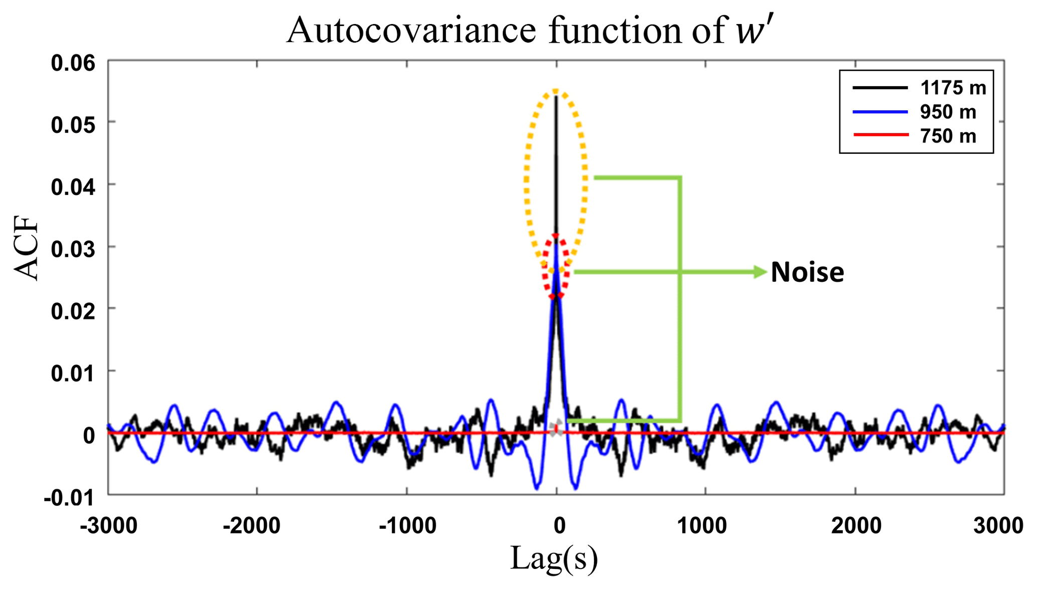
Figure 4Autocovariance function (ACF) of w′, obtained from Doppler lidar at three different heights on 19 May 2016 from 08:00–09:00 UTC in Granada.
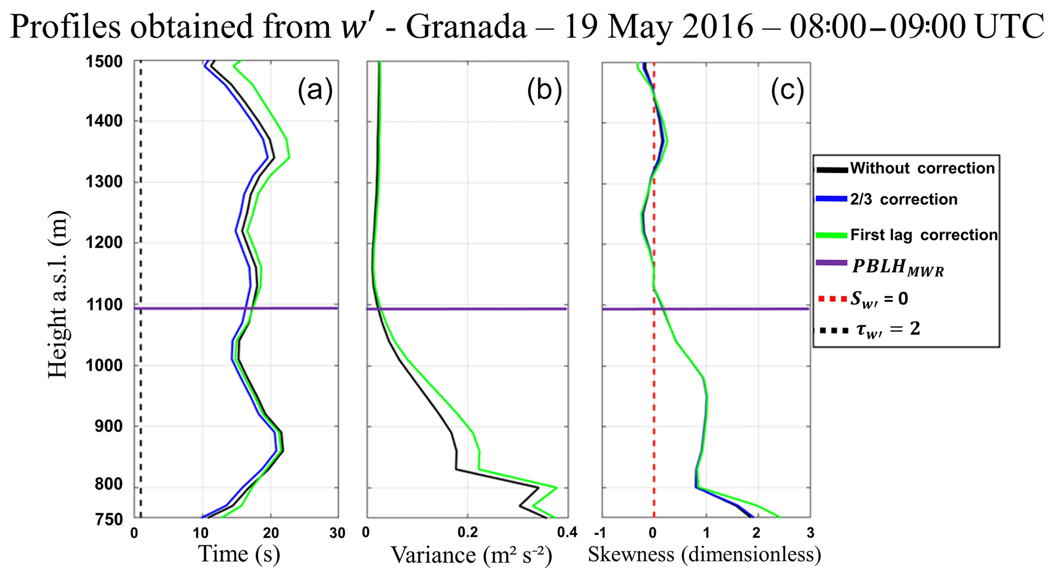
Figure 5(a) Vertical profile of integral timescale (). (b) Vertical profile of variance (). (c) Vertical profile of skewness (). All profiles were obtained from Doppler lidar data on 19 May 2016 from 08:00–09:00 UTC in Granada.
Figure 5a illustrates the comparison between the integral timescale () without correction and the two corrections cited in Sect. 3.2. Except for the first height bins, below the PBLHMWR, the profiles have little differences as well as small error bars. Above the PBLHMWR the first lag correction presents higher differences in relation to the other profiles at around 1350 m.
Figure 5b and c show the comparison of variance () and skewness (), respectively, with and without corrections. The profiles corrected by law correction do not present significant differences in comparison to uncorrected profiles. On the other hand, the profiles corrected by the first lag correction have slight differences below the PBLHMWR, mainly the ( only in the first 50 m). Therefore, considering high signal-to-noise ratio (SNR) conditions, although the presence of ε can slightly change the value of high-order moments, it is not enough to distort the observed phenomena, as shown by the impact of the corrections applied.
For EL we use the same procedure for the correction and error analysis that we apply to the DL data. The same day was chosen (19 May), however the period selected is between 12:00 and 13:00 UTC, due to the incomplete overlap of MULHACÉN.
In this sense, we studied the influence of noise at two wavelengths: 1064 nm, which has been previously analyzed by Pal et al. (2010), as presented in the Sect. 2 and adopted as a reference (considering the rather low impact of molecular signal and the two-way transmittance shown in Eq. 9), and 532 nm was only used in order to check the feasibility of this wavelength for turbulence studies considering its widespread use in observation networks (Pappalardo et al., 2014; Guerrero-Rascado et al., 2016). Figures 6 and 7 show the autocovariance function, obtained from and , respectively, at three distinct heights. As expected, ε increases with the range, principally above the PBLHMWR. However, the wavelength 532 nm is more influenced by the noise, which can be verified by the higher peak at lag 0 in Fig. 7, in comparison with peaks at same lag in Fig. 6.
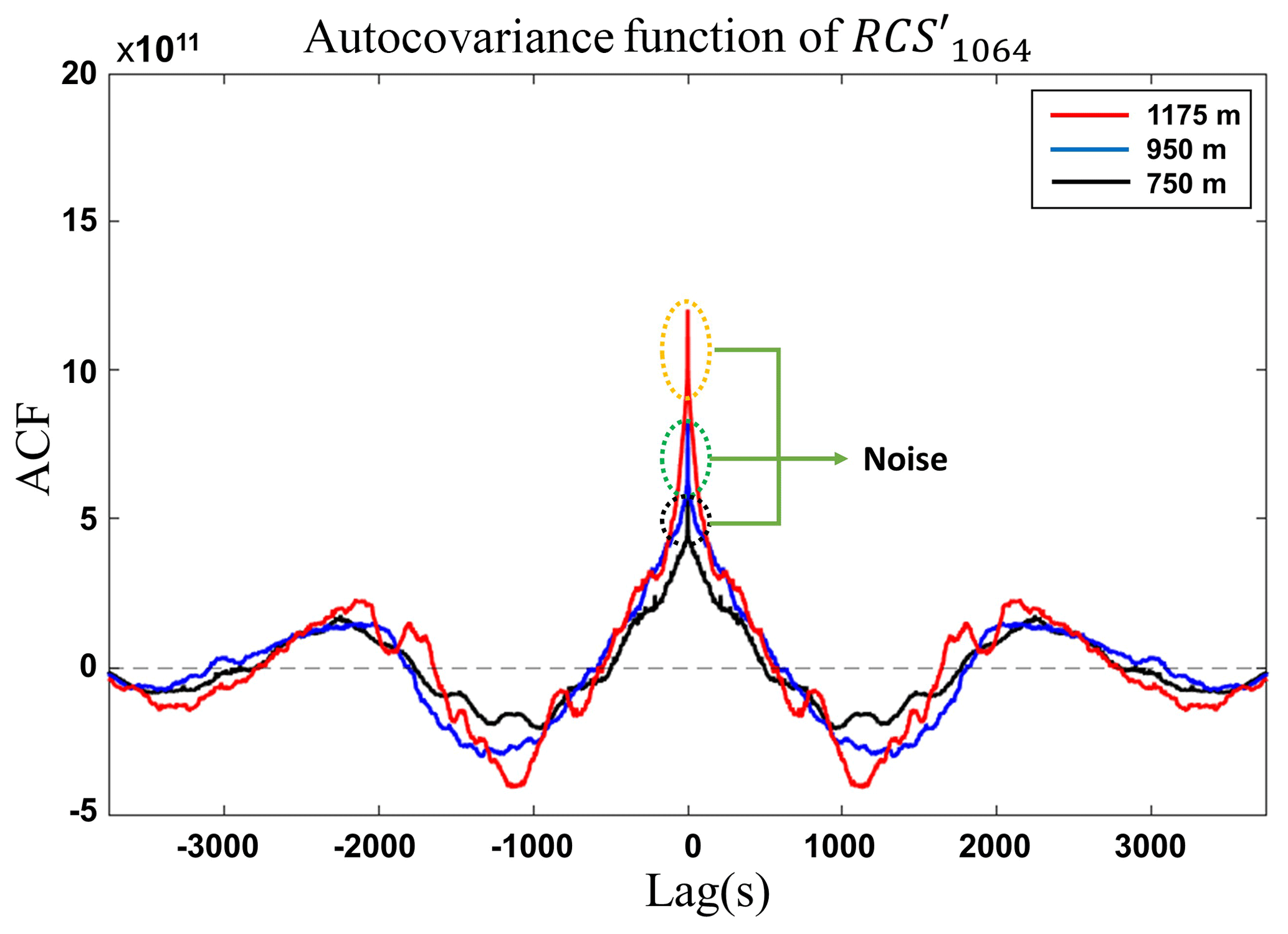
Figure 6Autocovariance of RCS′1064 obtained from MULHACÉN elastic lidar data for three different heights on 19 May 2016 from 12:00–13:00 UTC in Granada.
Although the level of influence of ε in each wavelength depends on the SNR of them (which is associated to technical factors such as laser output power, filters and the type of detectors), considering the proposed methodology, evaluating the composition of each wavelength is also important. The large contribution of to the total β at 532 nm, in comparison with the behavior at 1064 nm, can influence the results obtained from this wavelength, because our methodology is based on the use of . In addition, the larger extinction (due to both aerosol particles and molecules) at 532 nm produces a lower two-way transmittance, resulting in the reduction of the SNR values at this wavelength. Since we used the elastic lidar technique, we could not calculate aerosol extinction profiles, but an estimation of these transmittances was done on the basis of the Klett method (Klett, 1985). With this method, a constant lidar ratio value was constrained for each profile using the aerosol optical depth (AOD) derived from a collocated AERONET sunphotometer (Guerrero-Rascado et al., 2008). Using these constrained lidar ratios, the transmittances were calculated together with aerosol backscatter profiles, integrated up to 2.5 km. The estimated two-way transmittance was 0.85 for the case analyzed in this subsection (19 May).
Figure 8a, b, c and d show the vertical profiles of (a.u. – arbitrary units), , and kurtosis (), respectively, obtained at 1064 nm, with and without the corrections described in Sect. 3.2. In general, the corrections do not affect the profiles generated from 1064 nm data in a significant way, so the higher influence of corrections is observed in the profile, which is underestimated in some regions. In the Fig. 9a, b, c and d we show same high-order moments calculated from 532 nm data. As the complexity of moments increases, it is possible to observe the larger influence of the corrections, due to propagation of noise. Nonetheless, the application of the corrections, mainly the first lag correction, make these profiles very similar to those generated from the wavelength 1064 nm, so the same phenomena can be observed in both.
Therefore, in spite of the larger attenuation expected at 532 nm wavelength, which reduces the SNR of the profiles in comparison with 1064 nm, the application of the proposed corrections, mainly the first lag, reduces this influence significantly and enable the observation of the same phenomena detected in the high-order moments obtained from 1064 nm. Consequently, the wavelength 532 nm will be applied in the analysis presented in Sect. 4.2. The first lag correction was adopted as default due to it generates more relevant results in comparison with the law correction, providing a more careful analysis.
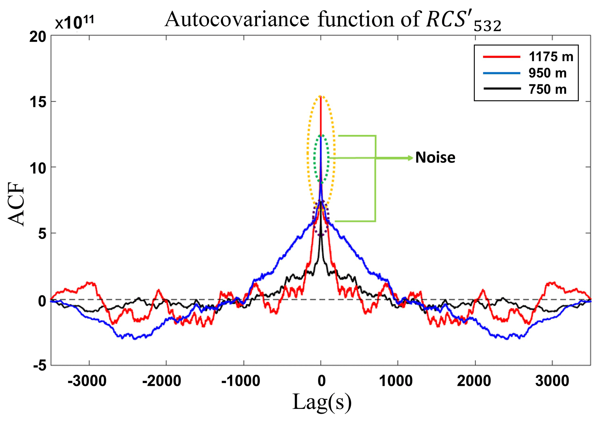
Figure 7Autocovariance of RCS′532 obtained from MULHACÉN elastic lidar data for three different heights on 19 May 2016 from 12:00–13:00 UTC in Granada.
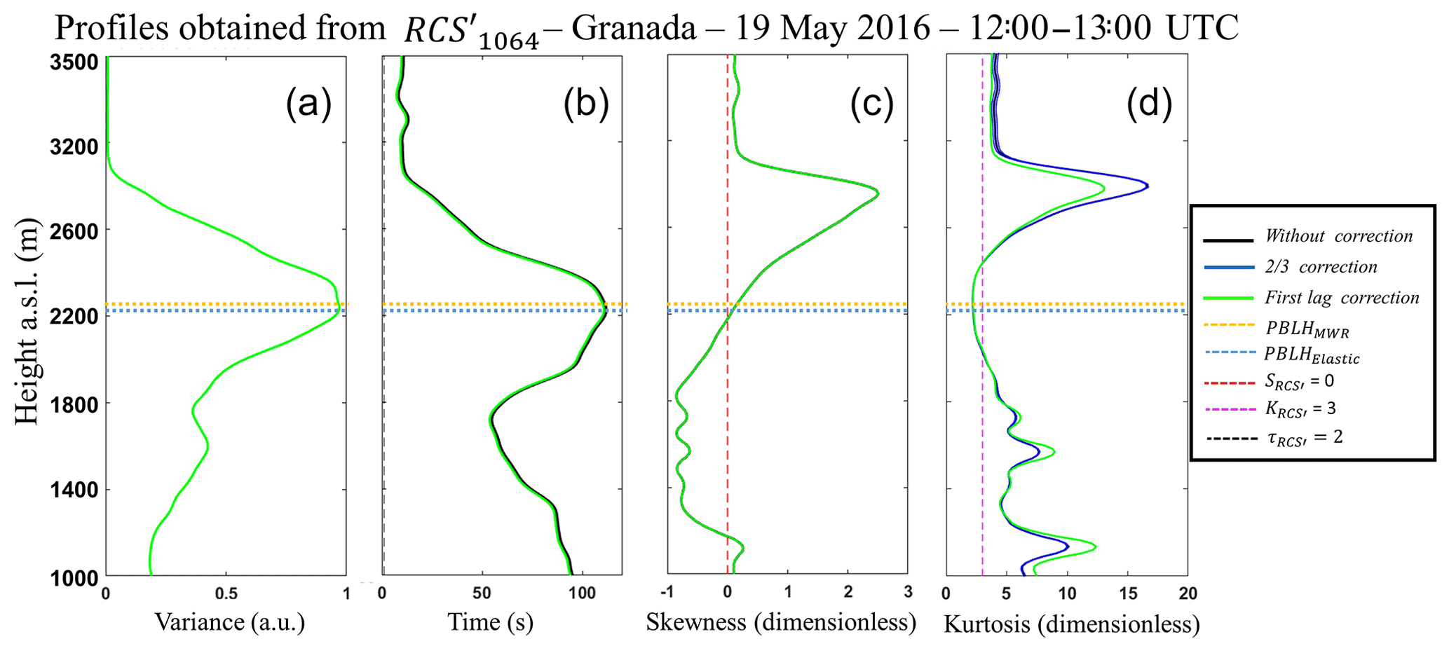
Figure 8(a) Vertical profile of variance (). (b) Vertical profile of integral timescale (). (c) Vertical profile of skewness (). (d) Vertical profile of kurtosis (). All profiles were obtained from MULHACÉN elastic lidar data on 19 May 2016 in Granada from 12:00–13:00 UTC.
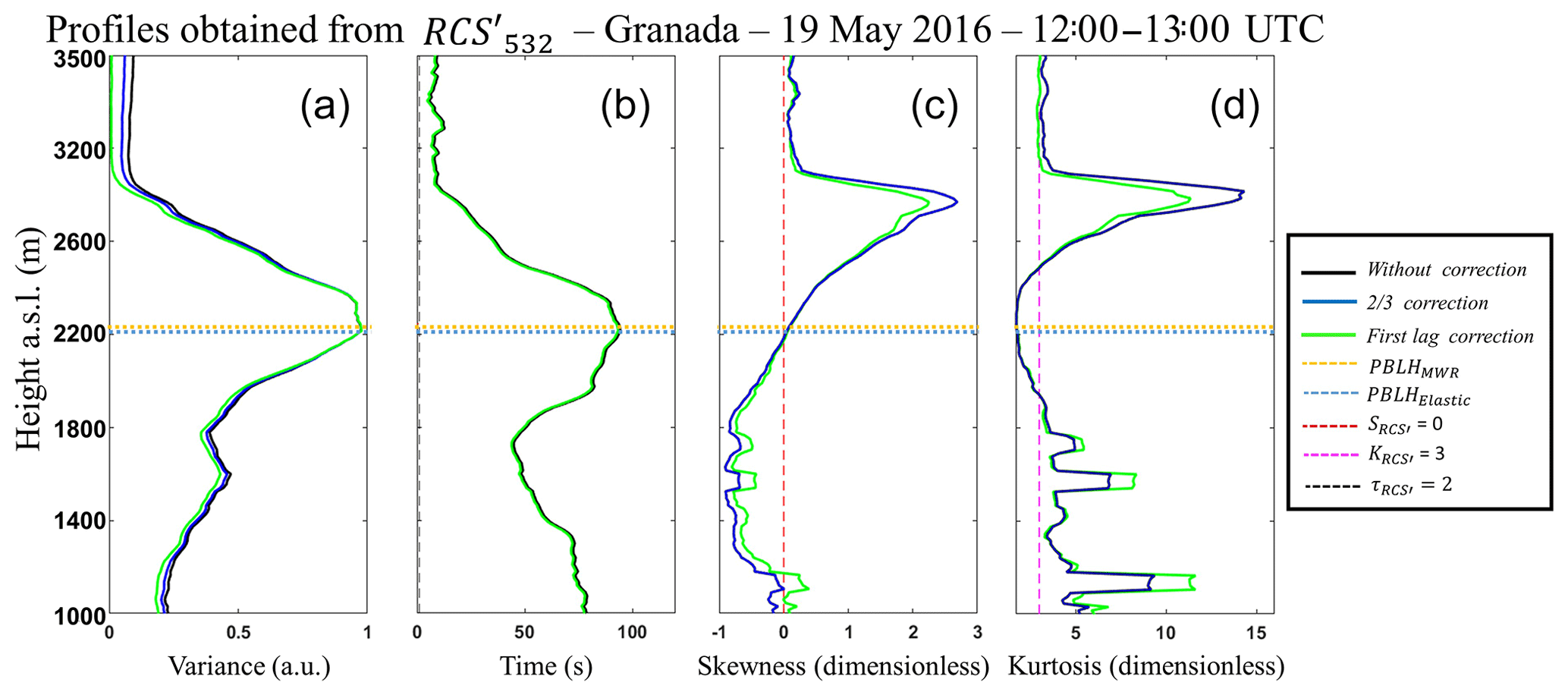
Figure 9(a) Vertical profile of variance (). (b) Vertical profile of integral timescale (). (c) Vertical profile of skewness (). (d) Vertical profile of kurtosis (). All profiles were obtained from MULHACÉN elastic lidar data on 19 May 2016 in Granada from 12:00–13:00 UTC.
4.2 Case studies
In this section we present two study cases in order to show how the products indicated in Table 2 can provide a detailed description about the turbulence in the PBL. The first case represents a typical day with a clear sky situation. The second case corresponds to a more complex situation, where there is presence of clouds and Saharan mineral dust layers.
Table 2Products and their respective meaning, provided by each system.

4.2.1 Case study I: clear sky situation
In this case study we use measurements gathered with DL, the MWR and the pyranometer over 24 h. The EL was operated under an operator-supervised mode between 08:20 to 18:00 UTC.
Figure 10a shows the integral timescale obtained from DL data (). The gray area represents the region where it is not possible to analyze the turbulent process from our DL data, either because of the low SNR values, which result in null values of the , or due to regions where the is not null but is lower than the acquisition time of the DL. However, the gray area is located almost entirely above the PBLHMWR (white stars).
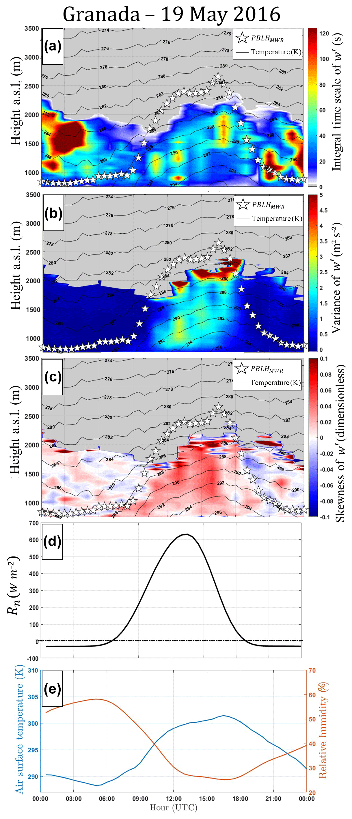
Figure 10(a) Integral timescale obtained from Doppler lidar data (), (b) variance obtained from Doppler lidar data (), (c) skewness obtained from Doppler lidar data (), (d) net radiation obtained from pyranometer data (Rn), and (e) air surface temperature (blue line) and surface relative humidity (RH – orange line) were both obtained from surface sensors. All profiles were acquired on 19 May 2016 in Granada. In (a), (b) and (c), black lines and white stars represent air temperature and PBLHMWR, respectively.
The has low values during the entire period when the SBL is present (Fig. 10b). Nevertheless, as air temperature begins to increase (around 07:00 UTC), the increases along with the PBLHMWR. The reaches its maximum values in the middle of the day, when we also observe the maximum values of air temperature and PBLHMWR. The combination of the and PBLHMWR provides us with better comprehension about the PBLH growth speed, so in the moments where high values of are observed, it means higher values of turbulent kinetic energy (TKE), which favor the fast ascension of PBLH.
The skewness of w′ () is shown in Fig. 11c. The describes the distribution of the turbulent velocities. Thus a positive implies strong but narrow updrafts surrounded by weaker but more widespread downdrafts, and vice versa for negative . Consequently, positive values (red regions) correspond with a surface-heating-driven boundary layer, while negative (blue regions) ones are associated to cloud-top longwave radiative cooling. During the stable period, there is predominance of low absolute values of . Nevertheless, as air temperature increases (transition from stable to unstable period), values begin to become larger. Air temperature begins to decrease around 18:00 UTC, and there is a reduction of , so the generation rate of convective turbulence decreases. Therefore, if the turbulence cannot be maintained against dissipation, then the CBL becomes an SBL covered by the RL. Thus, the reduction observed in the PBLHMWR is due to the detection of SBL height.
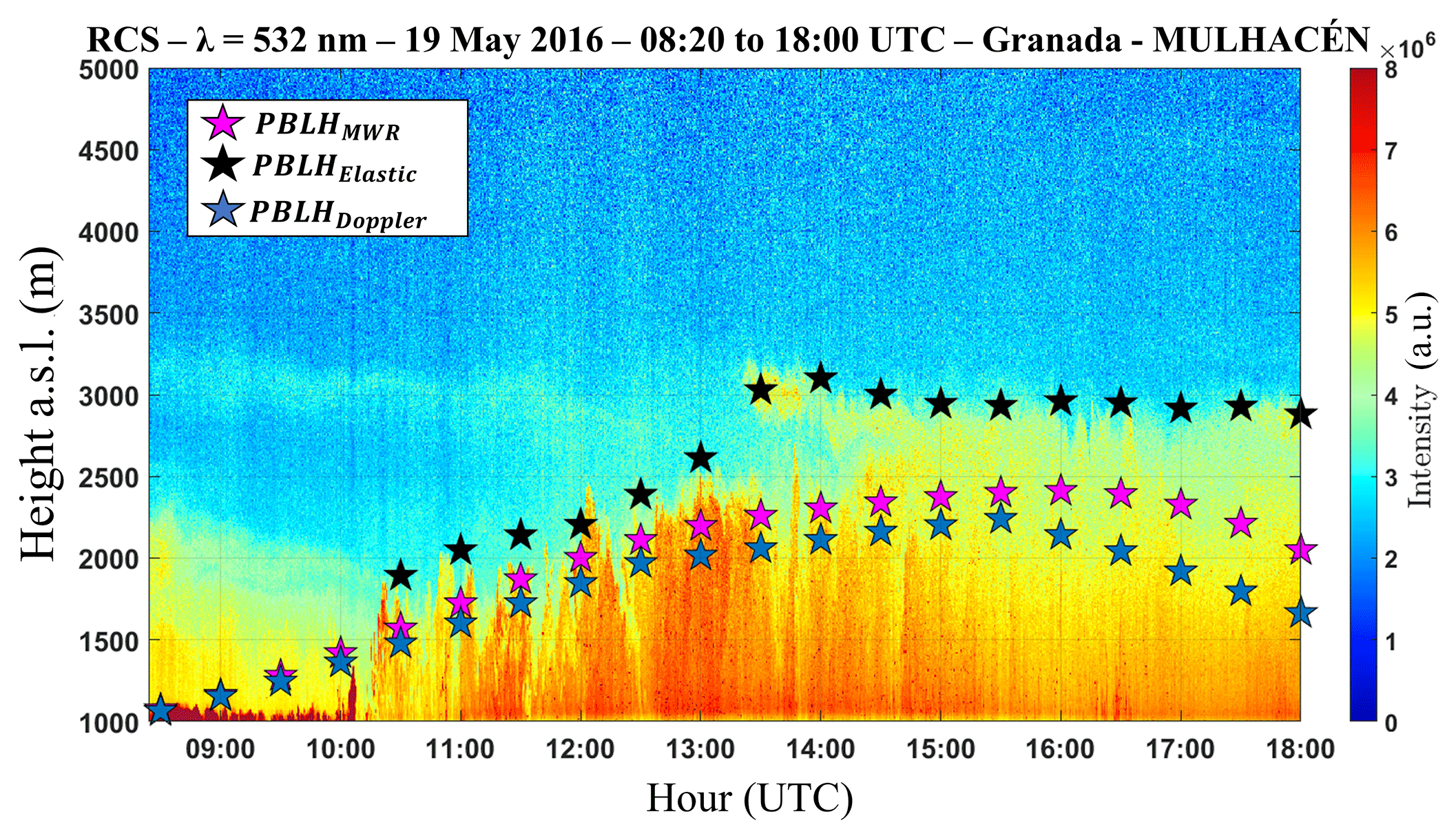
Figure 11Time–height plot of RCS obtained on 19 May 2016 in Granada. Pink stars represent the PBLHMWR, black stars represent the PBLHElastic and blue stars represent the PBLHDoppler.
Figure 10d shows the values of net surface radiation (Rn) that are estimated from solar global irradiance values using the seasonal model described in Alados et al. (2003). The negative values of Rn are concentrated in the stable region. The Rn begins to increase around 06:00 UTC and reaches its maximum in the middle of the day. Comparing Fig. 8c and d, we can observe similarity among the behavior of and Rn, so the joint analysis of these variables reinforce the characterization of this PBL as a surface-heating-driven CBL.
Figure 10e presents the values of surface air temperature and surface relative humidity (RH). Air surface temperature has a pattern of increase and decrease similar to that observed in Rn and . On the other hand, the RH is inversely correlated with temperature.
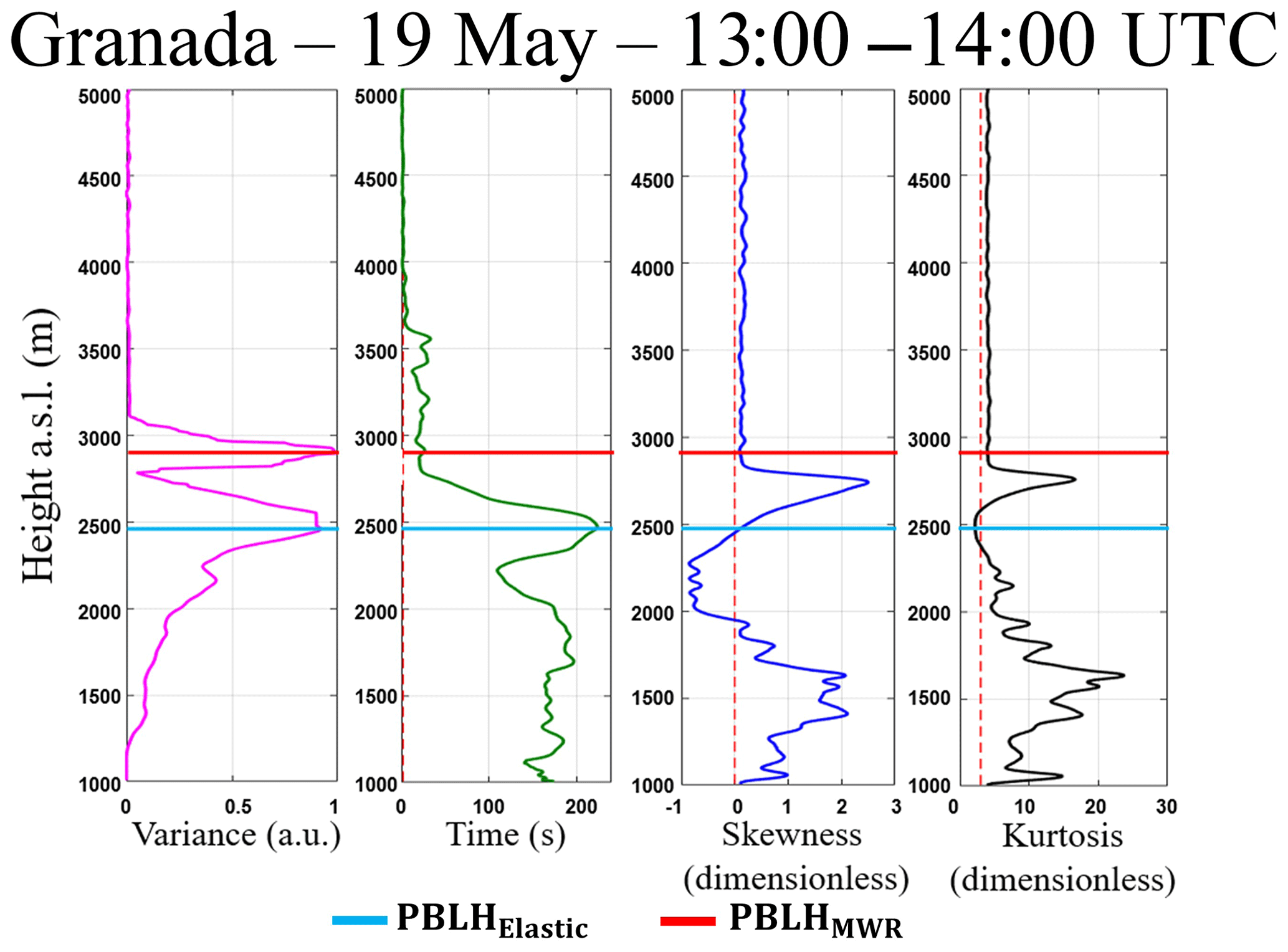
Figure 12Statistical moments obtained from 532 nm wavelength data of elastic lidar (MULHACÉN) in Granada from 13:00 to 14:00 UTC on 19 May 2016. From left to right is the variance (), integral timescale (]), skewness () and kurtosis ().
Figure 11 shows the RCS532 profile obtained from 08:00 to 18:00 UTC. At the beginning of the measurement period (08:20 to 10:00 UTC), observing the presence of a thin residual layer (around 2000 m a.s.l.) is possible, and later from 13:00 to 18:00 UTC, a lofted aerosol layer is evident. In this plot there are the PBLHMWR values (pink stars), the PBLHDoppler values (blue stars), obtained from the maximum of (Moreira et al., 2018), and the PBLHElastic values (black stars), obtained from the maximum of (Moreira et al., 2015). In the initial part of measurement, all profiles have similar behavior. However due to the distinct PBLH definition and tracer applied by each profile, the differences increase as CBL becomes more complex, e.g., with the presence of the lofted aerosol layer at 14:00 UTC. The joint observation of the results provided by these three methods can provide us information about the sub-layers in the PBL, both in convective and stable situations. Due to low variability of PBLH, the period between 13:00 and 14:00 UTC has been selected from the high-order moments to be analyzed.
Figure 12 presents the statistical moments generated from the RCS′ of wavelength 532 nm which were obtained between 13:00 and 14:00 UTC. The red line in all graphics represents the PBLHElastic (2200 m a.s.l.), and the blue one represents the average value of PBLHMWR (2250 m a.s.l.), both obtained between 13:00 and 14:00 UTC.
Due to the presence of a decoupled aerosol layer at 13:30 UTC, the average values of PBLHElastic and PBLHMWR have a difference of around 500 m. The has small and practically constant values between 1000 and 1400 m, evidencing the homogeneity of aerosol distribution in this region. From 1400 m the value of begins to increase, reaching a positive peak at PBLHMWR, which represents the entrainment zone (region characterized by an intense mixing between air parcels coming from the CBL and free troposphere – FT, causing a high variation in aerosol concentration). The PBLHElastic values observed at approximately 2900 m demonstrate an inherent difficulty of the variance method for detecting the PBLH in the presence of several aerosol layers (Kovalev and Eichinger, 2004). Above the PBLHElastic the values of decrease slowly due to location of the lofted aerosol around 2500 m. However, above this aerosol layer the value of is reduced to zero, indicating a large homogeneity in aerosol distribution at this region, which is expected, because the aerosol concentration at the FT is negligible in this case. The integral timescale obtained from RCS′ () has values higher than EL time acquisition throughout the CBL, evidencing the feasibility of studying turbulence using this elastic lidar configuration. The skewness values obtained from RCS′ () give us information about aerosol motion. The positive values of observed in the lowest part of profile and above the PBLHElastic represent the updrafts of aerosol layers. The negative values of indicate the region with low aerosol concentration due to clean air coming from the FT. This movement of the ascension of aerosol layers and the descent of clean air with a zero value of at PBLH (characteristic of the CBL growing) was also detected by Pal et al. (2010) and McNicholas and Turner (2014). The kurtosis of RCS′ () determines the level of mixing at different heights. There are values of larger than 3 in the lowest part of profile and around 2500 m, showing a peaked distribution in this region. On the other hand, values of lower than 3 are observed close to the PBLHElastic, therefore this region has a well-mixed CBL regime. Pal et al. (2010) and McNicholas and Turner (2014) also detected this feature in the region near the PBLH. In Fig. 13 the high-order moments obtained at the same period described above are shown, however they are shown from the 1064 nm data (our reference wavelength). It is possible to observe a similarity between the profiles obtained from each wavelength, so the same phenomena observed in the profiles generated from 532 nm and described above are also detected in the profiles obtained from the reference wavelength.
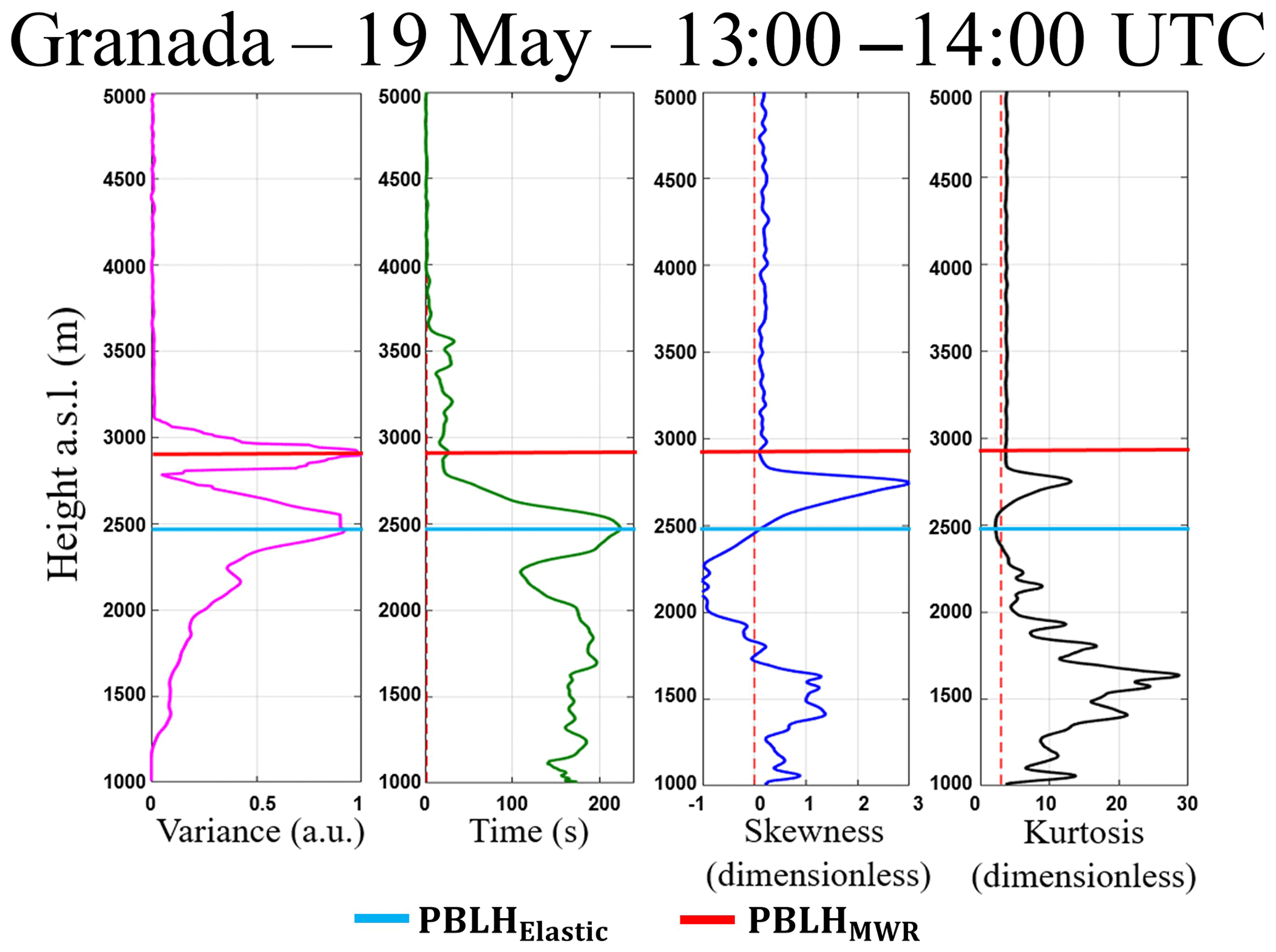
Figure 13Statistical moments obtained from 1064 nm wavelength data of elastic lidar (MULHACÉN) in Granada from 13:00–14:00 UTC on 19 May 2016. From left to right is the variance (), integral timescale (), skewness () and kurtosis ().
The results provided by DL, pyranometer and MWR data agree with the results observed in Figs. 12 and 13. In the same way, the analysis of high-order moments of RCS′ fully agree with the information in Fig. 10. Thus, the large values of and detected around 2500 m a.s.l, where we can see a lofted aerosol layer, suggest the ascent of an aerosol layer and the presence of a peaked distribution, respectively.
4.2.2 Case study: dusty and cloudy scenario
In case study measurements with DL, the MWR and pyranometer expand over 24 h, while EL data are collected from 09:00 to 16:00 UTC.
Figure 14a shows . Outside of the period from 13:00 to 17:00 UTC, the greatest part of gray area is situated above the PBLHMWR (white stars), thus DL time acquisition is enough to perform studies about turbulence in this case.
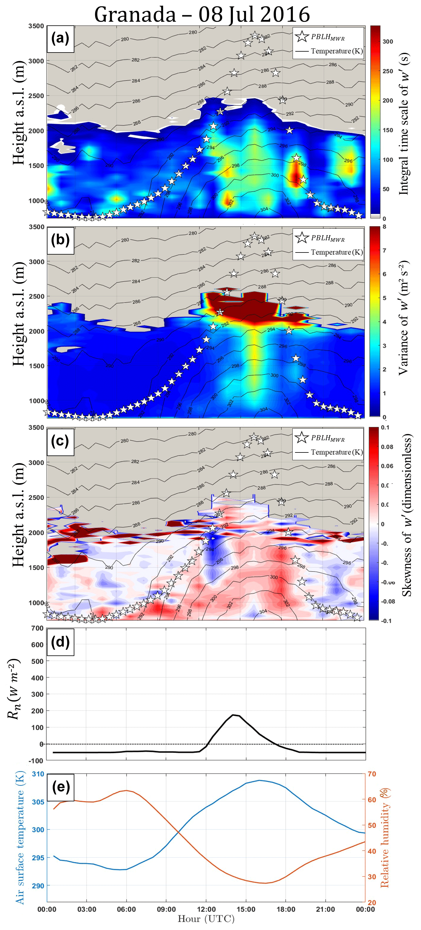
Figure 14(a) Integral timescale from Doppler lidar data (), (b) variance from Doppler lidar data (), (c) skewness from Doppler lidar data (), (d) net radiation from pyranometer data (Rn), and (e) air surface temperature (blue line) and surface relative humidity (RH – orange line) from surface sensor data. All profiles were obtained in Granada on 8 July 2016. In (a), (b) and (c), black lines and white stars represent air temperature and PBLHMWR, respectively.
has values close to zero during the entire stable period (Fig. 14b). However, when air temperature begins to increase (around 06:00 UTC), the also increases and reaches its maximum in the middle of the day. The higher values of PBL growth speed are observed in the moments where reaches its maximum values. In the late afternoon, as air temperature decreases, the values of (and consequently the TKE) decrease gradually until they reach the minimum value associated with the SBL. Figure 14c shows the profiles of . The main features of this case are the low values of , the slow increase and ascension of positive values, and the predominance of negative values from 12:00 to 13:00 UTC. The first two features are likely due to the presence of the intense Saharan dust layer (Fig. 15), which reduces the transmission of solar irradiance and consequently the absorption of solar irradiance at the surface, generating a weak convective process. From Fig. 16 we can observe the presence of both middle-altitude clouds and very intense dust layers from 12:00 to 15:00 UTC. This combination contributes to the intense negative values of the observed in this period until around 2 km, because, as mentioned previously, the is directly associated with the direction of turbulent movements, which can be characterized as cloud-top longwave radiative cooling during this period (Ansmann et al., 2010).
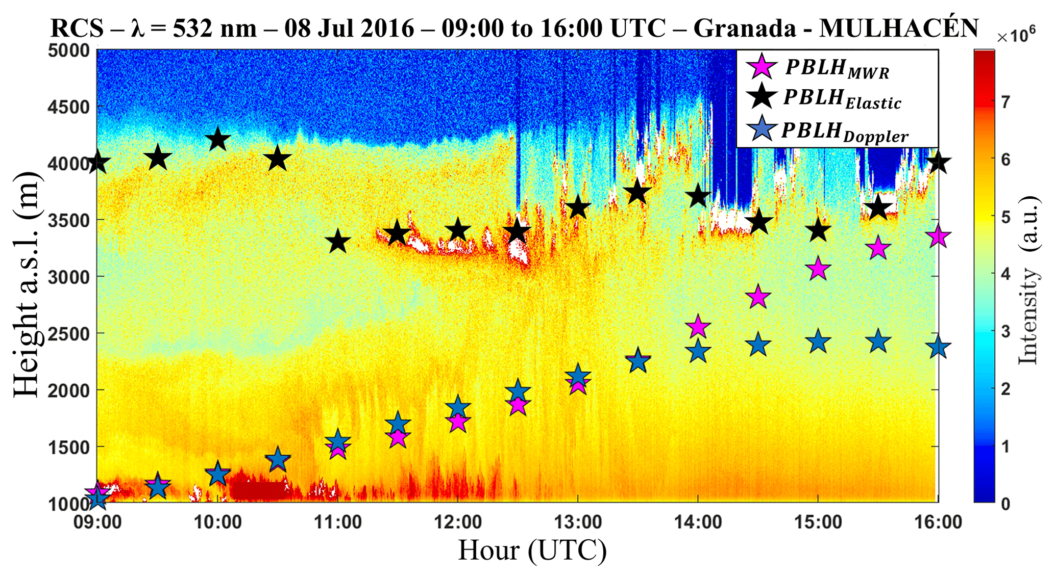
Figure 15Time–height plot of RCS obtained from MULHACÉN elastic lidar data on 8 July 2016 in Granada. Pink stars represent the PBLHMWR, black stars represent the PBLHElastic and blues stars represent the PBLHDoppler.
The influence of the Saharan dust layer can also be evidenced by the Rn pattern (Fig. 14d), which maintains negative values until 12:00 UTC and reaches a low maximum value (around 200 W m−2). The observation of and Rn between 12:00 and 14:00, as well as the presence of clouds and geometrically thick dust layers during this same period, reinforces the hypothesis of a case of the cloud-top longwave radiative cooling in the CBL. The air surface temperature and the RH (Fig. 14e) present the same correlation and anti-correlation (respectively) observed in the earlier case study, where the maximum of air surface temperature and the minimum of RH are detected in coincidence with the maximum daily value of PBLHMWR.
As mentioned before, Fig. 15 shows the RCS profile obtained from 09:00 to 16:00 UTC in a complex situation, with presence of the decoupled dust layer (around 3800 m a.s.l.) from 09:00 to 12:00 UTC and the presence of both middle-altitude clouds and very intense dust layers (around 3500 m a.s.l.) from 11:30 to 16:00 UTC. The pink, black and blue stars represent the PBLHMWR, PBLHDoppler and PBLHElastic, respectively. Due to the presence of dusty layers and clouds, the difference between the methods is more evident, mainly in the PBLHElastic, which uses aerosol as tracers. This method only produces results close to the others at 15:00 UTC, when the dust layer is mixed with the CBL.
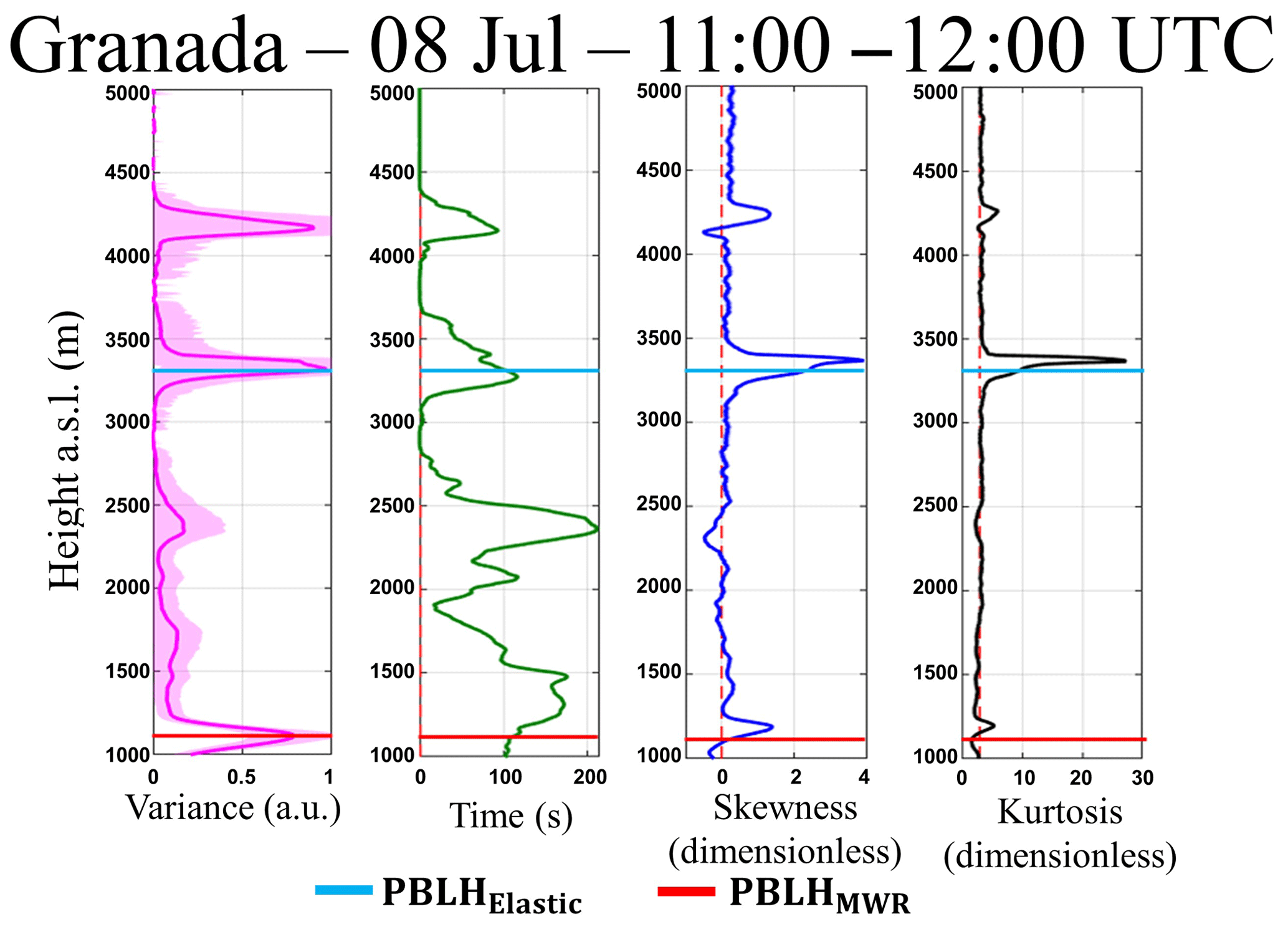
Figure 16Statistical moments obtained from 532 nm wavelength data of elastic lidar (MULHACÉN) in Granada from 11:00–12:00 UTC on 8 July 2016. From left to right is the variance (), integral timescale (), skewness () and kurtosis ().
Figure 16 illustrates the statistical moments of RCS′ of 532 nm wavelength obtained from 11:00 to 12:00 UTC. The profile presents several peaks due to the presence of distinct aerosol sub-layers. The first peak is coincident with the value of PBLHMWR. The value of PBLHelastic is coincident with the base of the dust layer. This difficulty of detecting the PBLH in presence of several aerosol layers is inherent in the variance method (Kovalev and Eichinger, 2004). However, the joint observation of PBLHMWR and PBLHelastic enables us to characterize and distinguish the several sub-layers. The values of are higher than EL acquisition time all along the PBL, evidencing the feasibility of EL time acquisition for studying the turbulence of PBL in this case. The profile has several positive values, due to the large number of aerosol sub-layers that are present. The characteristic inflection point of is observed to be coincident with the PBLHMWR, which confirms the agreement between this point and the PBLH. From the analysis of and , it is possible to justify these phenomena from the mixing process demonstrated in the earlier case study. The predominately has values lower than 3 below 2500 m, thus showing how this region is well mixed, as can be seen in Fig. 16. Values of larger than 3 are observed in the highest part of profile, where the dust layer is located.
In order to show the feasibility of 532 nm wavelength, in the Fig. 17 are presented the high-order moments obtained between 11:00–12:00 UTC from 1064 nm wavelength data. Although the error of obtained from 532 nm (pink shadow) is considerably higher than the error of same variable obtained from 1064 nm, all profiles are very similar, so that, the same phenomena can be observed in both graphics (Figs. 16 and 17).
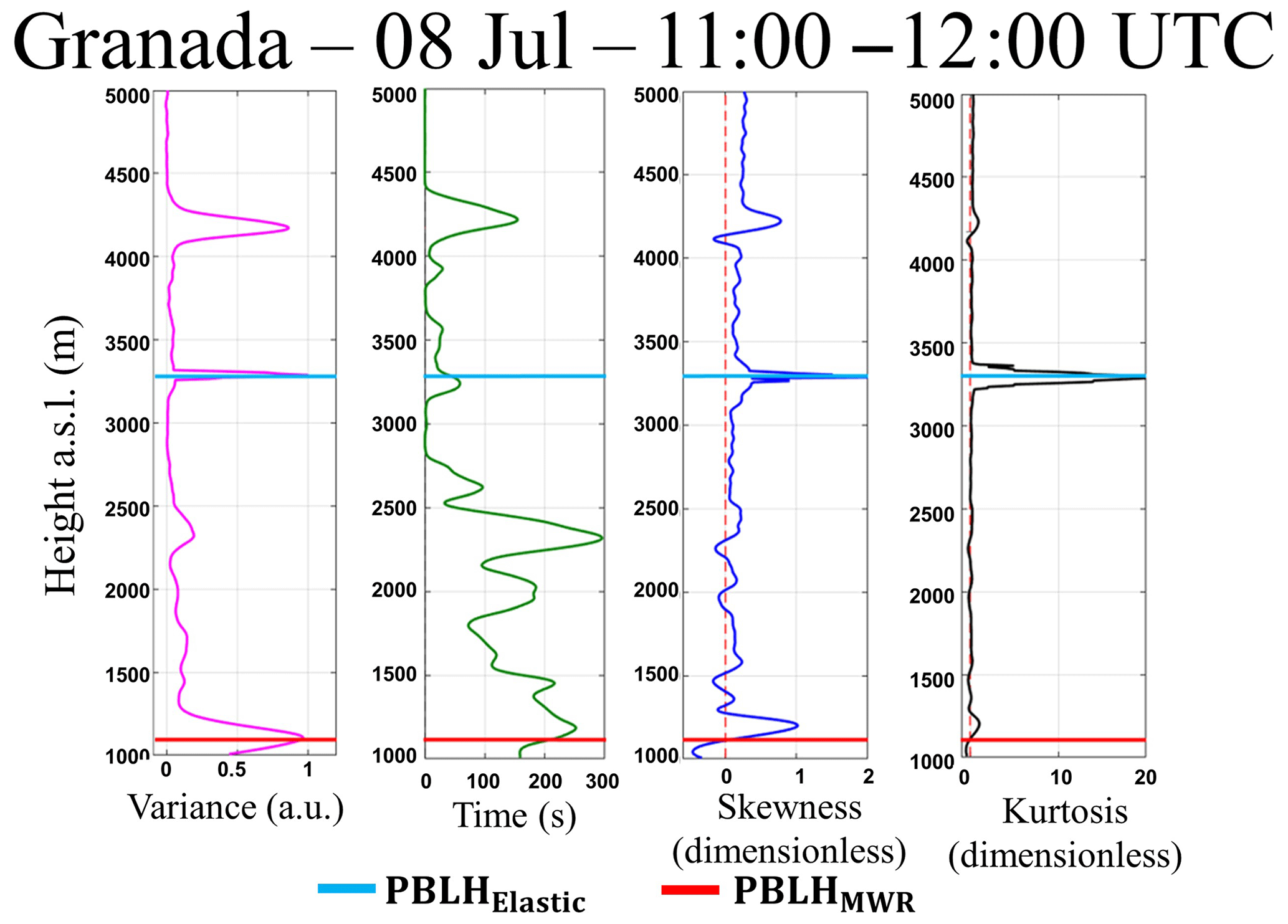
Figure 17Statistical moments obtained from 1064 nm wavelength data of elastic lidar (MULHACÉN) in Granada from 11:00–12:00 UTC on 8 July 2016. From left to right is the variance (), integral timescale (), skewness () and kurtosis ().
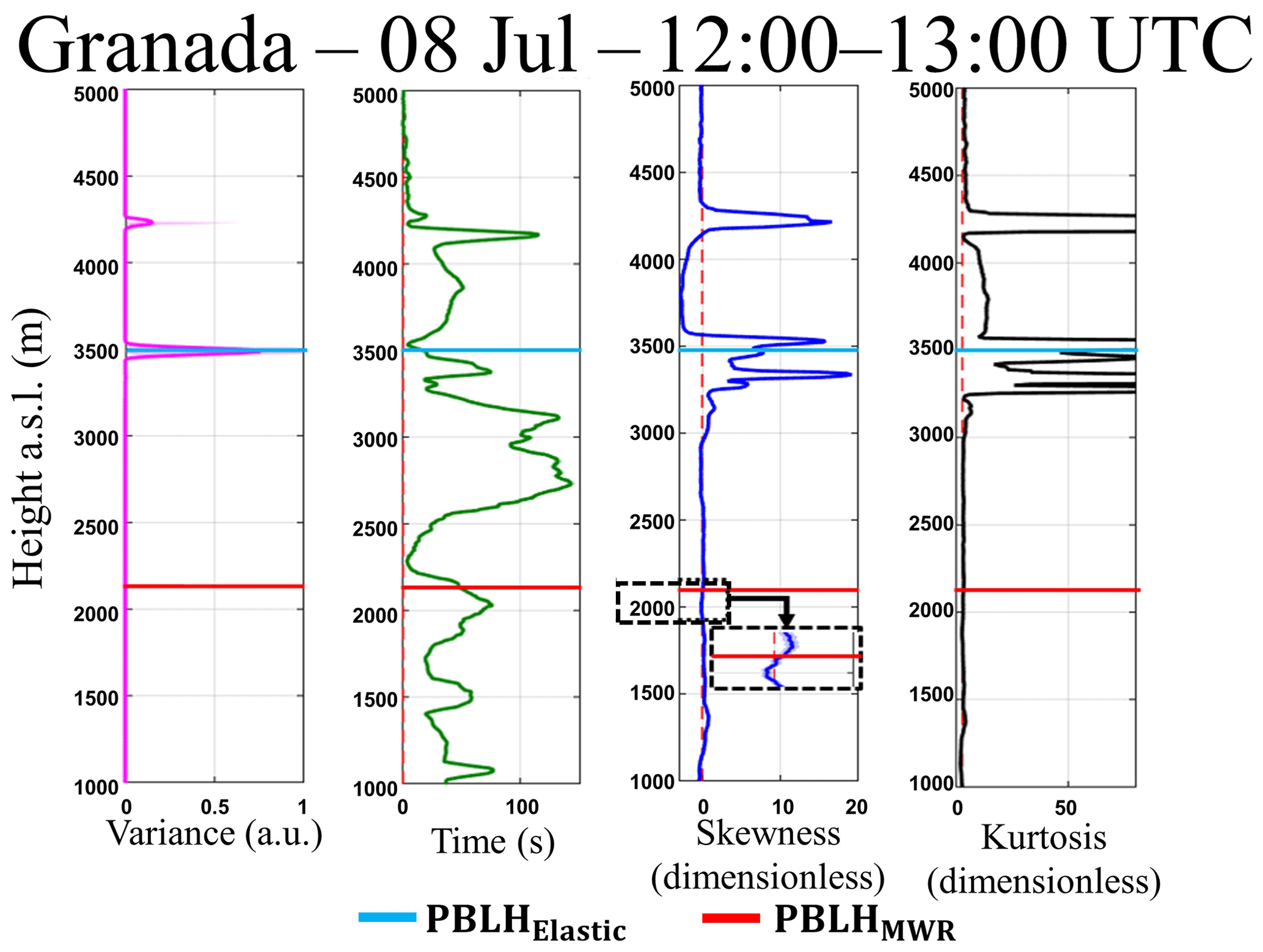
Figure 18Statistical moments obtained from 532 nm wavelength data of elastic lidar (MULHACÉN) in Granada from 12:00–13:00 UTC on 8 July 2016. From left to right is the variance (), integral timescale (), skewness () and kurtosis ().
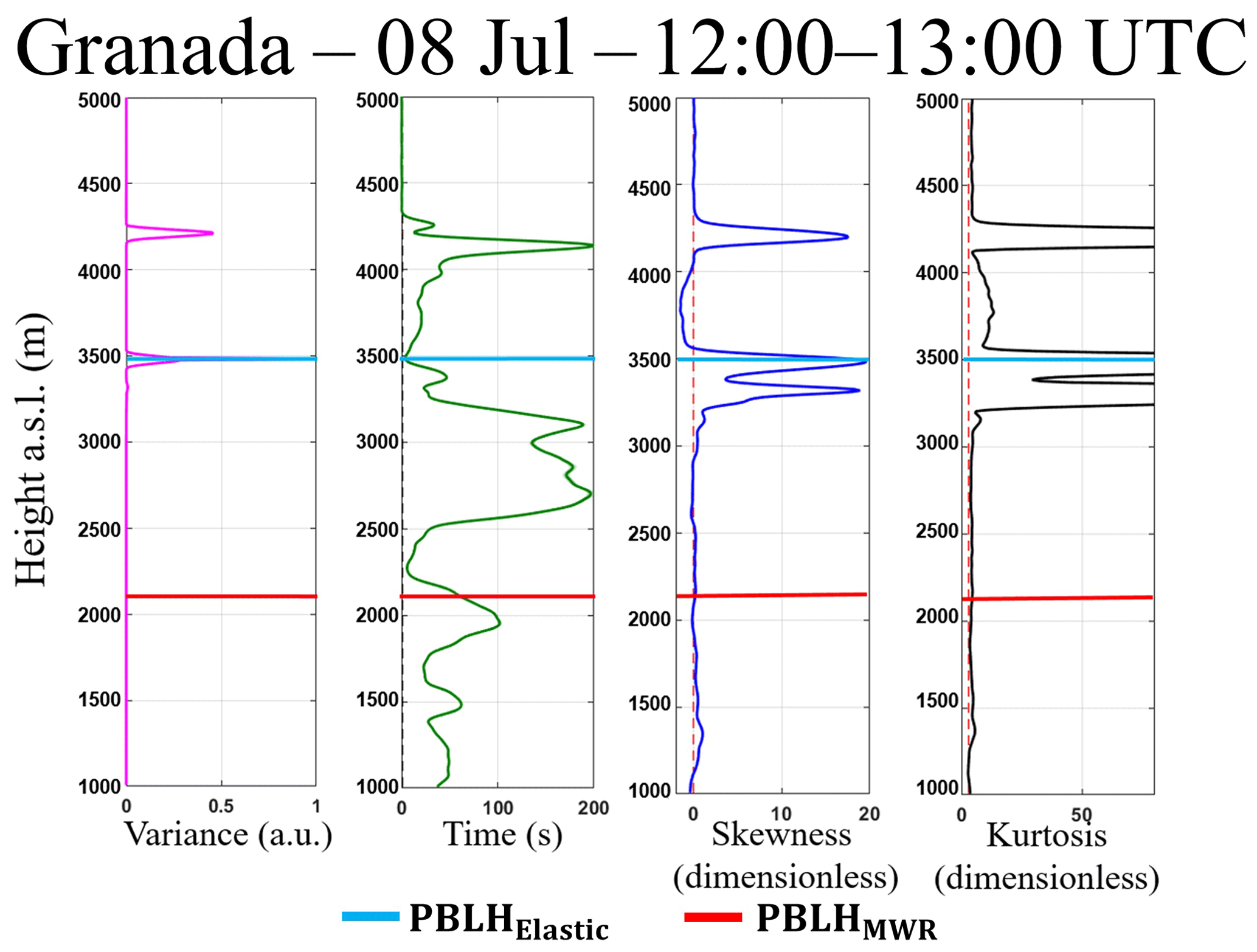
Figure 19Statistical moments obtained from 1064 nm wavelength data of elastic lidar (MULHACÉN) in Granada from 12:00–13:00 UTC on 8 July 2016. From left to right is the variance (), integral timescale (), skewness () and kurtosis ().
Figure 18 shows the RCS′ 532 nm wavelength high-order moments obtained from 12:00 and 13:00 in presence of cloud cover. The method based on the maximum of locates the PBLHElastic at the cloud base, due to the high variance of RCS′ generated by the clouds. The presents values larger than EL time acquisition, therefore this configuration enables us to study turbulence by EL analyses. The has few peaks, due to the mixing between CBL and dust layer that generates a more homogenous layer. The highest values of are observed in regions where there are clouds, and the negative values (between 3500 and 4000 m) occur due to presence of air from the FT between the two aerosol layers (Fig. 15). The inflection point of the profile is observed in the PBLHMWR region. The profile has low values in most of the PBL, demonstrating the high level of mixing during this period, where the dust layer and PBL are combined. The higher values of are observed in the region of clouds. In the same way as the previous analysis, the high-order moments of the period mentioned above were calculated for the wavelength of 1064 nm (Fig. 19). Although there are some differences in the absolute values of some profiles, the high-order moments generated using 1064 and 532 nm have similar profiles, so the same phenomena can be observed, demonstrating the viability of the 532 nm wavelength in the proposed methodology.
In this paper we perform an analysis of the PBL turbulent features from three different types of remote sensing systems (DL, EL and MWR) and surface sensors during the SLOPE-I campaign. We applied two kind of corrections to the lidar data: the first lag correction and law correction. The corrected DL statistical moments showed little variation with respect to the uncorrected profiles, denoting a rather low influence of the noise on high SNR conditions. The EL high-order moments were obtained from two wavelengths: 1064 nm, adopted as reference, and 532 nm, adopted in order to verify the viability to use the last one in turbulence analysis. From this comparison, it was possible to observe that the wavelength 532 nm is more affected by noise, in comparison with 1064 nm, due to the large contribution of the molecular component and the reduced two-way transmittance at that wavelength. However, the application of proposed corrections, mainly the first lag, can reduce this influence, so the same phenomena can be observed in the high-order moments provided from both wavelengths.
The case studies present two kind of situations: a well-defined PBL and a more complex situation with the presence of Saharan dust layer and some clouds. In both cases, it was possible to identify the events describe in Table 2. The combined use of remote sensing systems shows how the results provided by the different instruments can compliment each other, providing a detailed observation of some phenomena, mainly in complex situations.
Therefore, this study shows the feasibility of the described methodology based on the combination of remote sensing systems to retrieve a detailed picture on the PBL turbulent features. In addition, the feasibility of using the analyses of high-order moments of the RCS collected at 532 nm at a temporal resolution of 2 s offers the possibility of using the proposed methodology in networks such as EARLINET or LALINET with a reasonable additional effort.
Data used in this paper are available upon request from corresponding author (gregori.moreira@usp.br).
The supplement related to this article is available online at: https://doi.org/10.5194/acp-19-1263-2019-supplement.
The conceptualization was done by GdAM, JLGR and LAA. The methodology was done by GdAM and LAA. The software of analysis was developed by GdAM. The experiments were designed by GdAM, JLGR and LAA. The data acquisition was performed by GdAM, JLGR, JABO, POA, RR, AEBV and JABA. The formal analysis, investigation, writing of the original draft, preparation, review of the writing, and editing were performed by GdAM, JLGR, LAA, POA, FJOR and EL. The supervision, project administration and funding acquisition were done by LAA.
The authors declare that they have no conflict of interest.
This article is part of the special issue “EARLINET aerosol profiling: contributions to atmospheric and climate research”. It is not associated with a conference.
This work was supported by the Andalusia Regional Government through project
P12-RNM-2409 and by the Spanish Agencia Estatal de Investigación (AEI)
through projects CGL2016-81092-R and CGL2017-90884-REDT. We acknowledge the
financial support by the European Union's Horizon 2020 research and
innovation program through project ACTRIS-2 (grant agreement no. 654109). The
authors thankfully acknowledge the FEDER program for the instrumentation used
in this work and the University of Granada, which supported this study through
the Excellence Units Program and “Plan Propio. Programa 9 Convocatoria
2013”.
Edited by: Albert Ansmann
Reviewed by: two anonymous referees
Alados, I., Foyo-Moreno, I., Olmo, F. J., and Alados-Arboledas, L.: Relationship between net radiation and solar radiation for semi-arid shrub-land, Agr. Forest Meteorol., 116, 221–227, 2003.
Albrecht, B. A., Bretherton, C. S., Johnson, D., Scubert, W. H., and Frisch, A. S.: The Atlantic stratocumulus transition experiment – ASTEX, B. Am. Meteorol. Soc., 76, 889–904, 1995.
Andrews, E., Sheridan, P. J., Ogren, J. A., and Ferrare, R.: In situ aerosol profiles over the Southern Great Plains cloud and radiation test bed site: 1. Aerosol optical properties, J. Geophys. Res., 109, D06208, https://doi.org/10.1029/2003JD004025, 2004.
Ansmann, A., Fruntke, J., and Engelmann, R.: Updraft and downdraft characterization with Doppler lidar: cloud-free versus cumuli-topped mixed layer, Atmos. Chem. Phys., 10, 7845–7858, https://doi.org/10.5194/acp-10-7845-2010, 2010.
Antón, M., Valenzuela, A., Cazorla, A., Gil, J. E., Gálvez-Fernández, J., Lyamani, H., Foyo-Moreno, I., Olmo, F. J., and Alados-Arboledas, L.: Global and diffuse shortwave irradiance during a strong desert dust episode at Granada (Spain), Atmos. Res., 118, 232–239, 2012.
Bedoya-Velásquez, A. E., Navas-Guzmán, F., Granados-Muñoz, M. J., Titos, G., Román, R., Casquero-Vera, J. A., Ortiz-Amezcua, P., Benavent-Oltra, J. A., de Arruda Moreira, G., Montilla-Rosero, E., Hoyos, C. D., Artiñano, B., Coz, E., Olmo-Reyes, F. J., Alados-Arboledas, L., and Guerrero-Rascado, J. L.: Hygroscopic growth study in the framework of EARLINET during the SLOPE I campaign: synergy of remote sensing and in situ instrumentation, Atmos. Chem. Phys., 18, 7001–7017, https://doi.org/10.5194/acp-18-7001-2018, 2018.
Behrendt, A., Wulfmeyer, V., Hammann, E., Muppa, S. K., and Pal, S.: Profiles of second- to fourth-order moments of turbulent temperature fluctuations in the convective boundary layer: first measurements with rotational Raman lidar, Atmos. Chem. Phys., 15, 5485–5500, https://doi.org/10.5194/acp-15-5485-2015, 2015.
Bravo-Aranda, J. A., Navas-Guzmán, F., Guerrero-Rascado, J. L., Pérez-Ramírez, D., Granados-Muñoz, M. J., and Alados-Arboledas, L.: Analysis of lidar depolarization calibration procedure and application to the atmospheric aerosol characterization, Int. J. Remote Sens., 34, 3543–3560, 2013.
Caumont, O., Cimini, D., Löhnert, U., Alados-Arboledas, L., Bleisch, R., Buffa, F., Ferrario, M. E., Haefele, A., Huet, T., Madonna, F., and Pace, G.: Assimilation of humidity and temperature observations retrieved from ground-based microwave radiometers into a convective-scale NWP model, Q. J. Roy. Meteor. Soc., 142, 2692–2704, 2016.
Coen, M. C., Praz, C. Haefele, A., Ruffieux, D., Kaufmann, P., and Calpini, B.: Determination and climatology of the planetary boundary layer height above the Swiss plateau by in situ and remote sensing measurements as well as by the COSMO-2 model, Atmos. Chem. Phys., 14, 13205–13221, https://doi.org/10.5194/acp-14-13205-2014, 2014.
Engelmann, R., Wandinger, U., Ansmann, A., Müller, D., Žeromskis, E., Althausen, D., and Wehner, B.: Lidar Observations of the Vertical Aerosol Flux in the Planetary Boundary Layer, J. Atmos. Ocean. Tech., 25, 1296–1306, 2008.
Guerrero-Rascado, J. L., Ruiz, B., and Alados-Arboledas, L.: Multi-spectral lidar characterization of the vertical structure of Saharan dust aerosol over Southern Spain, Atmos. Environ., 42, 2668–2681, 2008.
Guerrero-Rascado, J. L., Olmo, F. J., Avilés-Rodríguez, I., Navas-Guzmán, F., Pérez-Ramírez, D., Lyamani, H., and Alados Arboledas, L.: Extreme Saharan dust event over the southern Iberian Peninsula in september 2007: active and passive remote sensing from surface and satellite, Atmos. Chem. Phys., 9, 8453–8469, https://doi.org/10.5194/acp-9-8453-2009, 2009.
Guerrero-Rascado, J. L., Costa, M. J., Bortoli, D., Silva, A. M., Lyamani, H., and Alados-Arboledas, L.: Infrared lidar overlap function: an experimental determination, Opt. Express, 18, 20350–20359, 2010.
Guerrero-Rascado, J. L., Landulfo, E., Antuña, J. C., Barbosa, H. M. J., Barja, B., Bastidas, A. E., Bedoya, A. E., da Costa, R. F., Estevan, R., Forno, R. N., Gouveia, D. A., Jimenez, C., Larroza, E. G., Lopes, F. J. S., Montilla-Rosero, E., Moreira, G. A., Nakaema, W. M., Nisperuza, D., Alegria, D., Múnera, M., Otero, L., Papandrea, S., Pawelko, E., Quel, E. J., Ristori, P., Rodrigues, P. F., Salvador, J., Sánchez, M. F., and Silva, A.: Latin American Lidar Network (LALINET) for aerosol research: diagnosis on network instrumentation, J. Atmos. Sol.-Terr. Phy., 138–139, 112–120, 2016.
Holzworth, G. C.: Estimates of mean maximum mixing depths in the contiguous United States, Mon. Weather Rev., 92, 235–242, https://doi.org/10.1175/1520-0493(1964)092<0235:EOMMMD>2.3.CO;2, 1964.
Illingworth, A. J., Hogan, R. J., O'Connor, E. J., Bouniol, D., Brooks, M. E., Delanoe, J., Donovan, D. P., Eastment, J. D., Gaussiat, N., Goddard, J. W. F., Haeffelin, M., Klein Baltink, H., Krasnov, O. A., Pelon, J., Piriou, J.-M., Protat, A., Russchenberg, H. W. J., Seifert, A., Tompkins, A. M., Van Zadelhoff, G.-J., Vinit, F., Willen, U., Wilson, D. R., and Wrench, C. L.: CLOUDNET: Continuous Evaluation of Cloud Profiles in Seven Operational Models using Ground-Based Observations, B. Am. Meteorol. Soc., 88, 883–898, https://doi.org/10.1175/BAMS-88-6-883, 2007.
Kaimal, J. C. and Gaynor, J. E.: The Boulder Atmospheric Observatory, J. Clim. Appl. Meteorol., 22, 863–880, 1983.
Kiemle, C., Brewer, W. A., Ehret, G., Hardesty, R. M., Fix, A., Senff, C., Wirth, M., Poberaj, G., and LeMone, M. A.: Latent heat flux profiles from collocated airborne water vapor and wind lidars during IHOP 2002, J. Atmos. Ocean. Tech., 24, 627–639, 2007.
Klett, J. D.: Lidar inversion with variable backscatter/extinction ratios, Appl. Optics, 24, 1638–1643, https://doi.org/10.1364/AO.24.001638, 1985.
Kovalev, V. A. and Eichinger, W. E.: Elastic Lidar, Wiley, 2004.
Lenschow, D. H., Wyngaard, J. C., and Pennell, W. T.: Mean-field and second-moment budgets in a baroclinic convective boundary layer, J. Atmos. Sci., 37, 1313–1326, 1980.
Lenschow, D. H., Mann, J., and Kristensen, L.: How long is long enough when measuring fluxes and other turbulence statistics?, J. Atmos. Ocean. Tech., 11, 661–673, 1994.
Lenschow, D. H., Wulfmeyer, V., and Senff, C.: Measuring second- through fourth-order moments in noisy data, J. Atmos. Ocean. Tech., 17, 1330–1347, 2000.
Lothon, M., Lenschow, D. H., and Mayor, S. D.: Coherence and scale of vertical velocity in the convective boundary layer from a Doppler lidar, Bound.-Lay. Meteorol., 121, 521–536, 2006.
Lyamani, H., Olmo, F. J., Alcántara, A., and Alados-Arboledas, L.: Atmospheric aerosols during the 2003 heat wave in southeastern Spain I: Spectral optical depth, Atmos. Environ., 40, 6453–6464, 2006.
McNicholas, C. and Turner, D. D.: Characterizing the convective boundary layer turbulence with a High Spectral Resolution Lidar, J. Geophys. Res.-Atmos., 119, 910–927, https://doi.org/10.1002/2014JD021867, 2014.
Monin, A. S. and Yaglom, A. M.: Statistical Fluid Mechanics, Vol. 2, MIT Press, 874 pp., 1979.
Moreira, G. de A., Marques, M. T. A., Nakaema, W., Moreira, A. C. d. C. A., and Landulfo, E.: Planetary boundary height estimations from Doppler wind lidar measurements, radiosonde and hysplit model comparisom, Óptica Pura y Aplicada, 48, 179–183, 2015.
Moreira, G. de A., Guerrero-Rascado, J. L., Bravo-Aranda, J. A., Benavent-Oltra, Ortiz-Amezcua, P., Róman, R., BedoyaVelásquez, A., Landulfo, E., and Alados-Arboledas, L.: Study of the planetary boundary layer by microwaveradiometer, elastic lidar and Doppler lidar estimations in Southern Iberian Peninsula, Atmos. Res., 213, 185–195, 2018.
Moreira, G. de A., Lopes, F. J. S., Guerrero-Rascado, J. L., Landulfo, E., and Alados-Arboledas, L.: Analyzing turbulence in Planetary Boundary Layer from multiwavelenght lidar system: impact of wavelength choice, Atmos. Meas. Tech. Discuss., in preparation, 2019.
Muppa, K. S., Behrendt, A., Späth, F., Wulfmeyer, V., Metzendorf, S., and Riede, A.: Turbulent humidity fluctuations in the convective boundary layer: Cases studies using water vapour differential absorption lidar measurements, Bound-Lay. Meteorol., 158, 43–66, https://doi.org/10.1007/s10546-015-0078-9, 2016.
Navas Guzmán, F., Guerrero Rascado, J. L., and Alados Arboledas, L.: Retrieval of the lidar overlap function using Raman signals, Óptica Pura y Aplicada, 44, 71–75, 2011.
Navas-Guzmán, F., Bravo-Aranda, J. A., Guerrero-Rascado, J. L., Granados-Muñoz, M. J., and Alados-Arboledas, L.: Statistical analysis of aerosol optical properties retrieved by Raman lidar over Southeastern Spain, Tellus B, 65, 21234, https://doi.org/10.3402/tellusb.v65i, 2013.
Navas-Guzmén, F., Fernández-Gálvez, J., Granados-Muñoz, M. J., Guerrero-Rascado, J. L., Bravo-Aranda, J. A., and Alados-Arboledas, L.: Tropospheric water vapour and relative humidity profiles from lidar and microwave radiometry, Atmos. Meas. Tech., 7, 1201–1211, https://doi.org/10.5194/amt-7-1201-2014, 2014.
O'Connor, E. J., Illingworth, A. J., Brooks, I. M., Westbrook, C. D., Hogan, R. J., Davies, F., and Brooks, B. J.: A method for estimating the turbulent kinetic energy dissipation rate from a vertically-pointing Doppler lidar, and independent evaluation from balloon-borne in-situ measurements, J. Atmos. Ocean. Tech., 27, 1652–1664, 2010.
Ortiz-Amezcua, P., Guerrero-Rascado, J. L., Granados-Muñoz, M. J., Bravo-Aranda, J. A., and Alados-Arboledas, L.: Characterization of atmospheric aerosols for a long range transport of biomass burning particles from canadian forest fires over the southern iberian peninsula in july 2013, Optica Pura y Aplicada, 47, 43–49, 2014.
Ortiz-Amezcua, P., Guerrero-Rascado, J. L., Granados-Muñoz, M. J., Benavent-Oltra, J. A., Böckmann, C., Samaras, S., Stachlewska, I. S., Janicka, L., Baars, H., Bohlmann, S., and Alados-Arboledas, L.: Microphysical characterization of long-range transported biomass burning particles from North America at three EARLINET stations, Atmos. Chem. Phys., 17, 5931–5946, https://doi.org/10.5194/acp-17-5931-2017, 2017.
Pal, S., Behrendt, A., and Wulfmeyer, V.: Elastic-backscatter-lidar-based characterization of the convective boundary layer and investigation of related statistics, Ann. Geophys., 28, 825–847, https://doi.org/10.5194/angeo-28-825-2010, 2010.
Pappalardo, G., Amodeo, A., Apituley, A., Comeron, A., Freudenthaler, V., Linné, H., Ansmann, A., Bösenberg, J., D'Amico, G., Mattis, I., Mona, L., Wandinger, U., Amiridis, V., Alados-Arboledas, L., Nicolae, D., and Wiegner, M.: EARLINET: towards an advanced sustainable European aerosol lidar network, Atmos. Meas. Tech., 7, 2389–2409, https://doi.org/10.5194/amt-7-2389-2014, 2014.
Román, R., Benavent-Oltra, J. A., Casquero-Vera, J. A., Lopatin, A., Cazorla, A., Lyamani, H., Denjean, C., Fuertes, D., Pérez-Ramirez, D., Torres, B., Toledano, C., Dubovik, O., Cachorro, V. E., Frutos, A. M., Olmo, F. J., and Alados-Arboledas, L.: Retrieval of aerosol profiles combining sunphotometer and ceilometer measurements in GRASP code, Atmos. Res., 204, 161–177, 2018.
Rose, T., Creewll, S., Löhnert, U., and Simmer, C.: A network suitable microwave radiometer for operational monitoring of cloudy atmosphere. Atmos. Res., 75, 183–200, 2005.
Stull, R. B.: An Introduction to Boundary Layer Meteorology, vol. 13, Kluwer Academic Publishers, the Netherlands, Dordrecht/Boston/London, 1988.
Stull, R. B.: Meteorology for Scientists and Engineers, 3rd Edn., Uni. Of British Columbia, 2011.
Stull, R. B., Santoso, E., Berg, L., and Hacker, J.: Boundary layer experiment 1996 (BLX96), B. Am. Meteorol. Soc., 78, 1149–1158, 1997.
Titos, G., Foyo-Moreno, I., Lyamani, H., Querol, X., Alastuey, A., and Alados-Arboledas, L.: Optical properties and chemical composition of aerosol particles at an urban location: An estimation of the aerosol mass scattering and absorption efficiencies, J. Geophys. Res.-Atmos., 117, D04206, https://doi.org/10.1029/2011JD016671, 2012.
Turner, D. D., Ferrare, R. A., Wulfmeyer, V., and Scarino, A. J.: Aircraft evaluation of ground-based Raman lidar water vapor turbulence profiles in convective mixed layers, J. Atmos. Ocean. Tech., 31, 1078–1088, https://doi.org/10.1175/JTECHD-13-00075.1, 2014.
Valenzuela, A., Olmo, F. J., Lyamani, H., Granados-Muñoz, M. J., Antón, M., Guerrero-Rascado, J. L., Quirantes, A., Toledano, C., Perez-Ramírez, D., and Alados-Arboledas, L.: Aerosol transport over the western mediterranean basin: Evidence of the contribution of fine particles to desert dust plumes over alborán island, J. Geophys Res., 119, 14028–14044, 2014.
van Ulden, A. P. and Wieringa, J.: Atmospheric boundary layer research at Cabauw, Bound.-Lay. Meteorol., 78, 39–69, 1996.
Vogelmann, A. M., McFarquhar, G. M., Ogren, J. A., Turner, D. D., Comstock, J. M., Feingold, G., Long, C. N., Jonsson, H. H., Bucholtz, A., Collins, D. R., Diskin, G. S., Gerber, H., Lawson, R. P., Woods, R. K., Andrews, E., Yang, H., Chiu, J. C., Hartsock, D., Hubbe, J. M., Lo, C., Marshak, A., Monroe, J. W., Mcfarlane, S. A., Jason, M., and Toto, T.: RACORO extended-term aircraft observations of boundary layer clouds, B. Am. Meteorol. Soc., 93, 861–878, https://doi.org/10.1175/BAMS-D-11-00189.1, 2012.
Williams, A. G. and Hacker, J. M.: The composite shape and structure of coherent eddies in the convective boundary layer, Bound.-Lay. Meteorol., 61, 213–245, 1992.
Wulfmeyer, V.: Investigation of turbulent processes in the lower troposphere with water vapor DIAL and radar-RASS, J. Appl. Sci., 56, 1055–1076, 1999.
Wulfmeyer, V., Pal., S., Turner, D. D., and Wagner, E.: Can water vapour Raman lidar resolve profiles of turbulent variables in the convective boundary layer?, Bound.-Lay. Meteorol., 136, 253–284, https://doi.org/10.1007/s10546-010-9494-z, 2010.