the Creative Commons Attribution 4.0 License.
the Creative Commons Attribution 4.0 License.
 | 09 Oct 2019
Evidence of small-scale quasi-isentropic mixing in ridges of extratropical baroclinic waves
Peter Hoor
Thorsten Kaluza
Jörn Ungermann
Björn Kluschat
Andreas Giez
Hans-Christoph Lachnitt
Martin Kaufmann
Martin Riese
Stratosphere–troposphere exchange within extratropical cyclones provides the potential for anthropogenic and natural surface emissions to rapidly reach the stratosphere as well as for ozone from the stratosphere to penetrate deep into the troposphere, even down into the boundary layer. The efficiency of this process directly influences the surface climate, the chemistry in the stratosphere, the chemical composition of the extratropical transition layer, and surface pollution levels. Here, we present evidence for a mixing process within extratropical cyclones which has gained only a small amount of attention so far and which fosters the transport of tropospheric air masses into the stratosphere in ridges of baroclinic waves. We analyzed airborne measurement data from a research flight of the WISE (Wave-driven ISentropic Exchange) campaign over the North Atlantic in autumn 2017, supported by forecasts from a numerical weather prediction model and trajectory calculations. Further detailed process understanding is obtained from experiments of idealized baroclinic life cycles. The major outcome of this analysis is that air masses mix in the region of the tropopause and potentially enter the stratosphere in ridges of baroclinic waves at the anticyclonic side of the jet without changing their potential temperature drastically. This quasi-isentropic exchange occurs above the outflow of warm conveyor belts, in regions which exhibit enhanced static stability in the lower stratosphere and a Kelvin–Helmholtz instability across the tropopause. The enhanced static stability is related to radiative cooling below the tropopause and the presence of small-scale waves. The Kelvin–Helmholtz instability is related to vertical shear of the horizontal wind associated with small-scale waves at the upper edge of the jet stream. The instability leads to the occurrence of turbulence and consequent mixing of trace gases in the tropopause region. While the overall relevance of this process has yet to be assessed, it has the potential to significantly modify the chemical composition of the extratropical transition layer in the lowermost stratosphere in regions which have previously gained a small amount of attention in terms of mixing in baroclinic waves.
- Article
(11159 KB) - Companion paper
- BibTeX
- EndNote


The extratropical transition layer (ExTL) as a unique feature of the extratropical upper troposphere and lower stratosphere (UTLS) is a direct consequence of the exchange and consequent mixing between air masses from the stratosphere and troposphere (e.g., Danielsen, 1968; Gettelman et al., 2011). The depth of this transition layer is commonly diagnosed from vertical distributions of trace species such as CO, O3, H2O, or N2O with either distinct tropospheric or stratospheric sources and from tracer–tracer correlations (e.g., Hoor et al., 2002; Pan et al., 2004). In the northern summer the ExTL extends up to 30 K in potential temperature above the local dynamic tropopause and between 20 and 25 K in all other seasons (Hoor et al., 2004). In the Southern Hemisphere, the ExTL seems to be more shallow (Hegglin et al., 2009).
The vertical distribution of trace species in the extratropical UTLS crucially depends on the large-scale stratospheric circulation (e.g., Butchart, 2014) and on stratosphere–troposphere exchange (STE) across the tropopause (e.g., Holton et al., 1995; Stohl et al., 2003; Sprenger et al., 2003). Overall, there are three prominent pathways for air into the ExTL. The stratospheric circulation contributes with two distinct branches distinguished based on the transit time between the major entry point of air into the stratosphere, i.e., the tropical tropopause, and the extratropics. The so-called deep branch, i.e., that associated with long transit times affects the ExTL through the descent of old stratospheric ozone-rich air into the UTLS. In contrast, the shallow branch with significantly shorter transit times introduces relatively young air from the tropical and subtropical UTLS into the extratropical UTLS (Birner and Bönisch, 2011). A recent study based on airborne measurements showed the effect of these two transport pathways on the changing abundance of carbon monoxide (CO) over the course of the Arctic winter in the ExTL (Krause et al., 2018). A third pathway into the ExTL is direct injection of extratropical tropospheric air into the stratosphere by troposphere-to-stratosphere transport (TST). These pathways all shape the vertical profiles of the trace species across the extratropical tropopause and thus can have an impact on the surface climate through a radiative feedback mechanism. Changes in the vertical abundance of radiatively active trace species in the UTLS, for instance for water vapor and ozone, have the relatively largest impact on the surface temperature (Riese et al., 2012).
Climatological studies revealed that in the Northern Hemisphere midlatitudes STE occurs predominantly in regions of enhanced cyclone activity, the storm tracks, over the North Atlantic and Pacific as well as over the Mediterranean Sea (Sprenger et al., 2003). Generally, in the extratropics STE occurs more frequently during winter and more mass is transported from the stratosphere into the troposphere, i.e., stratosphere-to-troposphere transport (STT) than vice versa, i.e., TST. This has recently been reported by Škerlak et al. (2014), who analyzed STE based on a 33-year-long time period of ERA-Interim reanalysis data and trajectory calculations. This analysis further confirmed earlier studies with respect to the spatial and temporal occurrence of STE (e.g., Chen, 1995; Morgenstern and Carver, 1999; Dethof et al., 2000). Also in a climatological sense the occurrence of STE in the extratropics is independent of the definition of the tropopause as shown by Boothe and Homeyer (2017) who used four different modern reanalysis data sets to analyze STE as well as first lapse rate (lrt1) and dynamic tropopause definitions.
Within the storm tracks Rossby waves are crucial for STE. During their life cycle, Rossby waves can lead to the formation of so-called stratospheric streamers and cut-off lows, both being regions of strong STE activity (Sprenger et al., 2007). STE also occurs in tropopause folds along jet streams due to the cross-frontal secondary circulation. Sprenger et al. (2003) demonstrated that exchange between subtropical and extratropical air masses across the subtropical jet predominantly occurs in these folds, but tropopause folds also exist at higher latitudes (Škerlak et al., 2015). Idealized simulations of baroclinic life cycles and analyses of reanalysis data showed that dynamic instabilities with low Richardson numbers, and thus large vertical shear of the horizontal wind, lead to mixing around tropopause folds (Bush and Peltier, 1994; Jaeger and Sprenger, 2007). Using similar data and methods to Škerlak et al. (2014), Reutter et al. (2015) studied the relevance of extratropical cyclones for STE over the North Atlantic. They found that the STT mass flux is generally larger than the TST mass flux and that the region of the exchange varies slightly during the life cycle of the cyclone. This study also confirmed earlier findings which suggested that STE occurs close to the cyclone center, or rather in regions with a relatively low tropopause height, and thus more on the cyclonic side of the jet in the region of the trough (e.g., Wernli and Davies, 1997).
An air parcel crossing the tropopause has to be affected by non-conservative processes which can modify its potential vorticity (Hoskins et al., 1985). Only then the air parcel can enter from a region with generally low potential vorticity (PV), i.e., the troposphere, into a region of high PV, i.e., the stratosphere, or vice versa. Lamarque and Hess (1994) differentiated between diabatic, i.e., potential temperature changing, and diffusive, i.e., related to friction, processes and showed that diabatic processes play a more vital role for STE than diffusive processes. Analyzing cross-tropopause transport in the UKMO model, Gray (2006) found similar results, with cloud and radiative processes being more important for STE than processes related to turbulence. In contrast, a recent study by Spreitzer et al. (2019) shows that turbulent processes are mainly responsible for changing the PV around the tropopause in a ridge of an extratropical baroclinic wave. They used high-resolution ECMWF forecast data and conclude that turbulence is evident around the jet stream. This turbulence is mainly related to the vertical shear of the jet stream but can also be caused by gravity waves (F. Zhang et al., 2015). Radiative effects may play an important role in anticyclones where radiation lowers the tropopause and thus leads to a mass flux from the troposphere into the stratosphere (Zierl and Wirth, 1997). Radiation is also a key process to dissolve stratospheric cut-off lows in the troposphere (Forster and Wirth, 2000). Clouds and related diabatic heating may also have an impact on STE. For instance warm conveyor belts, i.e., airstreams ahead of cold fronts associated with extratropical cyclones in which strong diabatic heating by latent heat release occurs (e.g., Wernli and Davies, 1997), can reach the upper troposphere and modify the PV, consequently allowing for exchange between tropospheric and stratospheric air (Wirth, 1995; Wernli and Bourqui, 2002). According to Spreitzer et al. (2019) clouds are more likely to change PV in regions with lower tropopause altitudes, e.g., in the trough. Similarly, rapid transfer from the boundary layer into the UTLS is evident in convective systems, which sometimes have the potential to overshoot into the stratosphere (e.g., Poulida et al., 1996; Stenchikov et al., 1996; Homeyer et al., 2014; Homeyer, 2015; Tang et al., 2011). Convection can also trigger gravity waves which occasionally break or dissipate and thus lead to small-scale mixing between tropospheric and stratospheric air masses (e.g., Whiteway et al., 2003). Jet-induced gravity waves might play a vital role for STE on small scales, inducing turbulence and consequently allowing for mixing between adjacent atmospheric layers (e.g., Langford et al., 1996; Lamarque et al., 1996). Strong shear zones are often apparent at the edges of the jet streams, which lead to filamentation of tropospheric or stratospheric air masses (Appenzeller et al., 1996). In these shear zones Kelvin–Helmholtz instabilities (KHIs) can emerge and lead to intense turbulence (e.g., Pepler et al., 1998; Whiteway et al., 2004). In turn this can lead to mixing of air masses around the jet streams. However, this mixing is thought to be more relevant at the lower edge (e.g., Danielsen, 1968; Shapiro, 1980) and on the cyclonic side of the jet and thus in the trough rather than in the ridge of baroclinic waves (e.g., Pan et al., 2007; Konopka and Pan, 2012).
Only a few studies focused on mixing and STE on the anticyclonic side of the jet in the ridges of baroclinic waves. Early suggestions were based on individual airborne observations with small-scale waves being responsible for cross-tropopause transport in these regions (Shapiro, 1980; Danielsen et al., 1991). Model simulations by Lamarque and Hess (1994) showed that PV is not conserved in the ridge of the studied baroclinic wave and that cloud-related processes lead to STE. Forster and Wirth (2000) showed how radiative effects can affect the tropopause altitude in anticyclones and thus lead to mass exchange from the troposphere into the stratosphere over the course of several days. Recently, Kunkel et al. (2016) showed that turbulent motions can occur on top of warm conveyor belt outflows at the altitude of the tropopause. This coincidence of turbulence in a region of the so-called tropopause inversion layer (TIL; Birner et al., 2002) addresses an open question with regard to the extratropical UTLS which is particularly relevant for the ExTL: does STE occur and does it affect the formation of the ExTL in the ridge of baroclinic waves where the static stability is usually strong in the extratropical lowermost stratosphere?
This study picks up the idea of turbulent mixing in regions of enhanced lower stratospheric static stability, which initially resulted from experiments of baroclinic life cycles (Kunkel et al., 2016) and which has recently been described by Kaluza et al. (2019) in composites of baroclinic waves over the North Atlantic. Birner et al. (2002) and Grise et al. (2010) both discussed that enhanced values of static stability and shear zones emerge close to each other at the tropopause level. Y. Zhang et al. (2015) addressed this further by linking the enhanced wind shear to propagating inertia-gravity waves with the potential to induce mixing without, however, addressing the larger scale meteorological conditions explicitly.
In this study we aim to analyze whether those turbulent signatures lead to mixing and potential exchange of tropospheric and stratospheric air masses in the ridge of baroclinic waves. For this we use complementary data of airborne measurements, numerical weather forecast data, trajectory calculations, and idealized baroclinic life cycle experiments which are introduced in Sect. 2. We will first focus on a research flight from the Wave-driven ISentropic Exchange campaign (Sect. 3), which aimed to measure chemical constituents and state parameters across the tropopause in a baroclinic wave over the North Atlantic. We then extend a set of well known idealized simulations of baroclinic life cycles to analyze STE and to obtain a comprehensive understanding of the processes which lead to mixing and potential STE in the ridge (Sect. 4). We finalize our study with a summary and a conclusion in Sect. 5.
2.1 Measurements during the WISE campaign 2017
In autumn 2017 the airborne research mission Wave-driven ISentropic Exchange (WISE) took place from Oberpfaffenhofen, Germany, and Shannon, Ireland, with the German HALO (High Altitude LOng Range) research aircraft. The main goals of the mission were to examine mixing processes in the UTLS in association with Rossby wave breaking and to study the impact of the Asian Summer Monsoon circulation on the budget of radiatively active species in the lower stratosphere. One specific target was to study the relation between the lower stratospheric static stability and cross-tropopause exchange in the extratropics.
During WISE, HALO was equipped with a unique set of instruments for in situ and remote sensing measurements. In this study we use in situ measurements of CO and N2O, and potential temperature Θ. CO and N2O have been measured with the University of Mainz Airborne Quantum Cascade Laser Spectrometer (UMAQS). The instrument is based on direct absorption spectroscopy using a continuous-wave quantum cascade laser with a sweep rate of 2 kHz (Müller et al., 2015). For the WISE campaign the total drift-corrected uncertainty was determined to be 0.94 ppbv for CO and 0.18 ppbv for N2O. Basic state parameters such as temperature, pressure, the three-dimensional wind vector, and others were measured with Basic HALO Measurement and Sensor System (BAHAMAS). The system is part of the basic aircraft and consists of a data acquisition system and a suite of sensors for basic meteorological and aerodynamic measurements. The system also contains interfaces into several aircraft systems like the inertial reference unit or the air data computer in order to monitor aircraft state parameters (Krautstrunk and Giez, 2012). The nose boom of HALO is part of this system and carries the air data probe for pressure and air flow measurements which are needed for determination of the wind vector. Additional BAHAMAS installations are six total air temperature (TAT) housings on the aircraft nose which can be used for temperature measurements and as inlets for sensors inside the nose. Two of these housings contain an open wire PT100 resistance thermometer for atmospheric temperature measurements, thus providing redundancy for this important parameter. The basic frequency for all atmospheric units is 100 Hz; data are usually processed on a 10 Hz basis. The accuracy of the pressure measurement is 0.3 hPa while the accuracy of the static temperature measurement is 0.5 K. We also use remote sensing measurements from the Gimballed Limb Observer for Radiance Imaging of the Atmosphere (GLORIA), which provides profile information of temperature and static stability, in addition to numerous trace gases (not used in this study). GLORIA is an airborne infrared limb imager combining a two-dimensional infrared detector with a Fourier transform spectrometer (Friedl-Vallon et al., 2014; Riese et al., 2014). The viewing direction is to the right of flight direction and depending on flight altitude and flight direction GLORIA observes the atmosphere between about 5 km and flight altitude with a vertical sampling of about 150 m at a tangent altitude of 10 km. The vertical resolution of retrieved temperature profiles and static stability is of the order of 300 m. The horizontal sampling along the flight track is up to 2 km (Kaufmann et al., 2015; Ungermann et al., 2015).
In total the WISE campaign comprised more than 140 flight hours during 15 research flights between 12 September 2017 and 21 October 2017. All flights except the first two started in Shannon, Ireland, and covered the North Atlantic between Greenland, Newfoundland, the Azores, and Europe as well as continental western and northern Europe. HALO was mostly flying in the UTLS up to ceiling altitudes of about 15 km, which corresponds to maximum potential temperature values of about 405 K and minimum pressure values of 130 hPa. The goal of research flight 07 (RF07) on 28 September 2017 was to study the abundance of trace species in the extratropical tropopause region. In particular, in accordance with the major goals of the WISE mission, the focus of this flight was on whether the trace species show specific signs of recent STE in regions of enhanced values of static stability in the lower stratosphere. Furthermore, the design of this flight was chosen such that the predictions of the idealized simulations of Kunkel et al. (2016) could be supported by observations. Thus, the flight was planned in the ridge of a synoptic-scale baroclinic wave which evolved during the previous days over the North Atlantic at the edge of a larger scale trough. A detailed description of the synoptic situation and the flight path will be given in Sect. 3.1.
2.2 ECMWF forecast data
We use forecast data from the European Centre for Medium-Range Weather Forecasts (ECMWF) to support the analysis of the airborne measurements and to provide more background information about the synoptic situation. We choose to use forecast data from ECMWF because they are available hourly at a very fine horizontal resolution. The forecast starts at 28 September 2017 00:00 UTC and we use the first 36 hourly steps until 29 September 2017 12:00 UTC. These data are used for analysis along the flight path where the full resolution is used corresponding to regular longitude–latitude grid spacing of about 0.07∘. Moreover, we use a slightly degraded data set with a horizontal grid spacing of 0.125∘ in the horizontal for a trajectory analysis. The forecast data have 137 vertical hybrid pressure-sigma levels up to 0.01 hPa with a vertical spacing of roughly 300 m in the UTLS.
2.3 Idealized baroclinic life cycle experiments
We complement our analysis of the airborne measurements using results from idealized baroclinic life cycle experiments. We continue the work of Kunkel et al. (2016) using the same setup of the COSMO (COnsortium for Small-scale MOdelling; Steppeler et al., 2003) model but extend the analysis with a more specific focus to analyze STE. For this we included additional artificial tracers to mark air masses which are initially located either in the troposphere or in the stratosphere, separated by the dynamic tropopause for which we use the isosurface of 2 pvu (1 pvu K m2 kg−1 s−1). Moreover, we included a tracer which is passively advected and which carries the information of the initial value of potential vorticity. With this tracer it is possible to determine how much PV in each model box has changed by diabatic processes since model start (Kunkel et al., 2014). Evaluating the difference between the current PV and the advected initial PV at the dynamic tropopause therefore allows regions of TST and STT to be detected.
We then repeated simulations from Kunkel et al. (2016) which included parameterizations for large-scale and convective clouds, radiation, and turbulence which have been labeled with BRTC (bulk microphysics, radiation, turbulence, and convection) by these authors. The model grid has a regular horizontal grid spacing of 0.4∘ in longitude and latitude and a vertical grid spacing of 110 m in the UTLS. Since the meteorological situation during RF07 was dominated by a wave-breaking event strongly resembling life cycle 1 (LC1), we will focus our discussion in Sect. 4 to results from LC1 experiments (Thorncroft et al., 1993), but we note that we also conducted simulations of life cycle 2 (LC2). Moreover, the LC2 experiments qualitatively gave the same results as the LC1 experiments. More information about the model setup and physics is given in Appendix A.
2.4 Trajectory calculations with LAGRANTO
The Lagrangian analysis tool (LAGRANTO; Sprenger and Wernli, 2015) allows calculating trajectories using the kinematic wind from four-dimensional meteorological data. It is possible to use both ECMWF and COSMO data as input for the trajectory calculations. The first trajectory analysis is based on ECMWF forecast data, which provides wind fields every hour. Trajectories have been initialized along the flight path with the goal of obtaining a more comprehensive picture of the temporal evolution of the meteorological parameters of the measured air masses. We will give more details on the trajectory start points and the analysis in Sect. 3.3.
For the second trajectory analysis we use COSMO wind fields. COSMO output is available every hour on a horizontal grid with spacing of 0.4∘ and a vertical spacing of about 110 m in the UTLS, thus providing a high-resolution input grid for the trajectory calculations. Based on the COSMO model output the goal of the trajectory calculations is to identify regions of cross-tropopause transport in the baroclinic life cycle experiments and whether exchange trajectories are evident in the ridge of the baroclinic wave. More details will be given in Sect. 4.
In general, we identify the exchange of air masses between the stratosphere and troposphere by the evolution of PV along a trajectory. If the PV of an air parcel increases from values below 2 pvu to values above this threshold, we mark this trajectory as a TST trajectory and vice versa for STT.
Finally, note that in this study discussion around static stability is usually associated with the first lapse rate tropopause, while discussion about STE is linked to the dynamic tropopause. Thus, both definitions will be considered in the analysis; however, if only the term tropopause is used, then we refer to the dynamic tropopause with a value of 2 pvu throughout the paper.
3.1 Synoptic situation and flight plan of WISE RF07
WISE RF07 targeted a fast-evolving baroclinic wave which emerged at the southern tip of a large-scale trough in the central North Atlantic in the early hours of 27 September 2017. While the large-scale trough traveled relatively slowly over the North Atlantic, the small-scale wave evolved rather fast, with the formation of a warm sector and well defined upper tropospheric fronts within 24 h as indicated by the PV at 330 K at 15:00 UTC on 28 September 2017 (Fig. 1a).
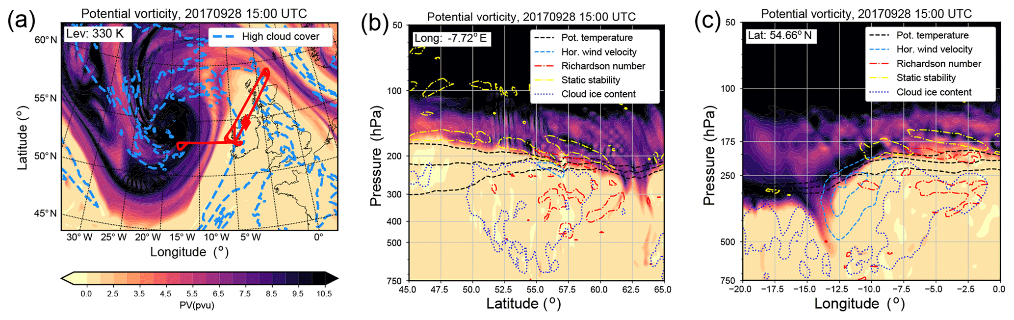
Figure 1Synoptic situation during WISE RF7 over the western North Atlantic at 15:00 UTC on 28 September 2017. (a) Potential vorticity on the isentropic surface of 330 K with high cloud cover (isoline showing a value of 0.9). (b) Meridional cross section of potential vorticity along −7.72∘ E longitude and (c) zonal cross section along 54.66∘ N latitude. The cross sections also show isolines of potential temperature (black dashed; 330, 335, 340 K), of horizontal wind velocity (light blue dashed; 45, 55 m s−1), the Richardson number (red dashed–dotted; 1), static stability (yellow dashed–dotted; s−2), and cloud ice content (blue dotted; kg kg−1). The cross sections are along the meridian and the circle of latitude of the red diamond shown in panel (a). This point also marks the location where the picture in Fig. 2b is taken.
The flight focused on the rapidly evolving ridge, which was expected to be strongly affected by diabatic processes and the vertical transport of boundary layer air in the region of the warm conveyor belt (WCB) ahead of the surface cold front. This system was expected to be situated close to Ireland in the afternoon hours of 28 September 2017. Take-off of WISE RF07 was at 13:15 UTC with a total flight time of 7 h 47 min. The flight strategy was twofold: first, staggered flight levels at FL400 (northeastward), FL380 (southwestward), FL360 (northeastward), FL340 (southwestward), FL420 (northeastward), and FL450 (southwestward) through the ridge of the baroclinic wave and second a survey of the stratospheric air with large PV values above the occlusion of the baroclinic wave west of Ireland (see also flight path in Figs. 1a and 2a). The intention of the first part in the northernmost part of the ridge of the baroclinic wave was to conduct co-located measurements of atmospheric state parameters and trace species across the local tropopause. The staggered flight level allowed these quantities to be measured in situ at different altitudes below, at, and above the level of the tropopause. From the highest flight levels (FL420 and FL450) in cloud-free conditions, two-dimensional distributions of temperature and trace species along the flight track were remotely measured with GLORIA. Our analysis focuses on the first part of the RF07, in particular on the first flight leg in the southwestward direction at FL380 (see Fig. 2a).
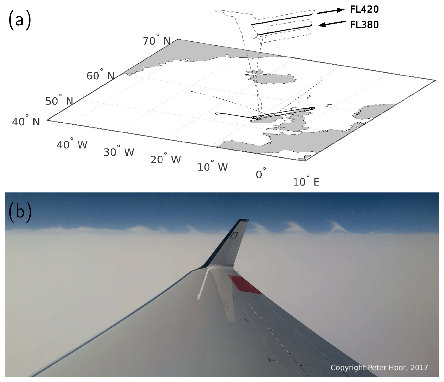
Figure 2(a) Three-dimensional flight track of WISE RF07, highlighting the flight legs important for this study. The arrows point in the direction of the flight on the respective levels. The dashed lines on the surface map show the angle of view of the photo shown in panel (b). (b) Photo taken on board HALO at 15:03 UTC during WISE RF07 showing Kelvin–Helmholtz cloud billows on top of a cirrus cloud deck.
A large part of the first leg of FL380 in the southwesterly direction was just above a widespread cirrus cloud deck associated with the upper tropospheric outflow of the WCB of the low pressure system. The high cloud cover in Fig. 1a shows the location of this cloud deck. The WCB also manifests itself in the low values of PV in the upper troposphere in the region where the ice clouds reach up to the tropopause (Fig. 1b, c). PV values are close to 0 pvu or even slightly below, which is common in such a situation due to a decreasing heating rate above the level of maximum heating (e.g., Chagnon et al., 2013; Joos and Wernli, 2012).
In the lower stratosphere the PV shows enhanced variability above the WCB outflow region (Fig. 1b, c). There are also high values of static stability evident, with values reaching as high as s−2. However, these high values emerge rather as wave-like patches and not as a layer. In between the high values the static stability has rather tropospheric background values (see also Fig. 3). More so, this region also exhibits low values of the Richardson number, indicative of Kelvin–Helmholtz instability and thus turbulence. Such a co-located enhancement of static stability and presence of turbulence was also evident in the life cycle experiments of Kunkel et al. (2016) and has recently been reported by Kaluza et al. (2019) based on a composite analysis of baroclinic waves over the North Atlantic.
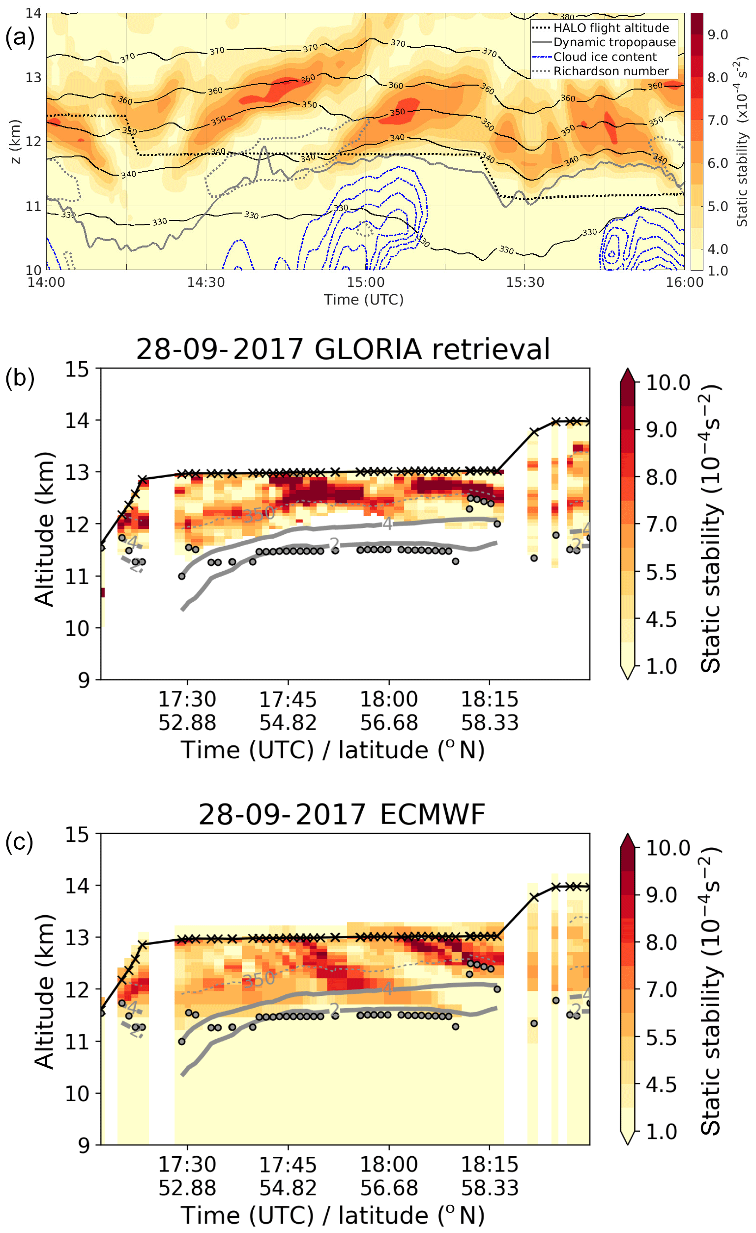
Figure 3(a) Static stability along the flight path between 14:00 and 16:00 UTC (color-shaded) along with potential temperature (black solid), cloud ice water content (blue dashed), the altitude of the dynamic tropopause (gray solid), and the Richardson number smaller than 1 (gray dotted) based on ECMWF forecast data. Black dotted line shows the altitude of HALO. (b) Static stability at GLORIA tangent points between 17:20 and 18:20 UTC. Black line shows the flight altitude with black crosses marking points of measurement. Thick gray lines show 2 and 4 pvu, thin gray line the 350 K isentrope based on ECMWF forecast data. Gray dotted points mark the location of the first lapse rate tropopause. (c) ECMWF forecast data sampled at GLORIA tangent points.
Another indication of turbulence in the region above the cloud deck stems directly from observations of Kelvin–Helmholtz cloud billows close to the flight path (Fig. 2b). A photo was taken at 15:03 UTC in a northwestern direction (Fig. 2a, diamond in Fig. 1a, b). The billows are indicative of a KHI which is thought to favor mixing of adjacent atmospheric layers and thus affects the vertical gradient of trace species. Notably, since the KHI emerges in the vicinity of the tropopause, it could potentially lead to STE. Commonly, a critical Richardson number of 0.25 identifies a KHI. However, in a non-convective situation such small Richardson numbers rely on large vertical shear of the horizontal wind. In turn, models based on a discretized grid with a grid spacing of a few hundred meters or more in the vertical can often not resolve the vertical shear sufficiently. In the region of the observed cloud billows we find Richardson numbers in the ECMWF model of about 1. We therefore use a Richardson number equal to 1 as a proxy for KHI in the UTLS for our analysis.
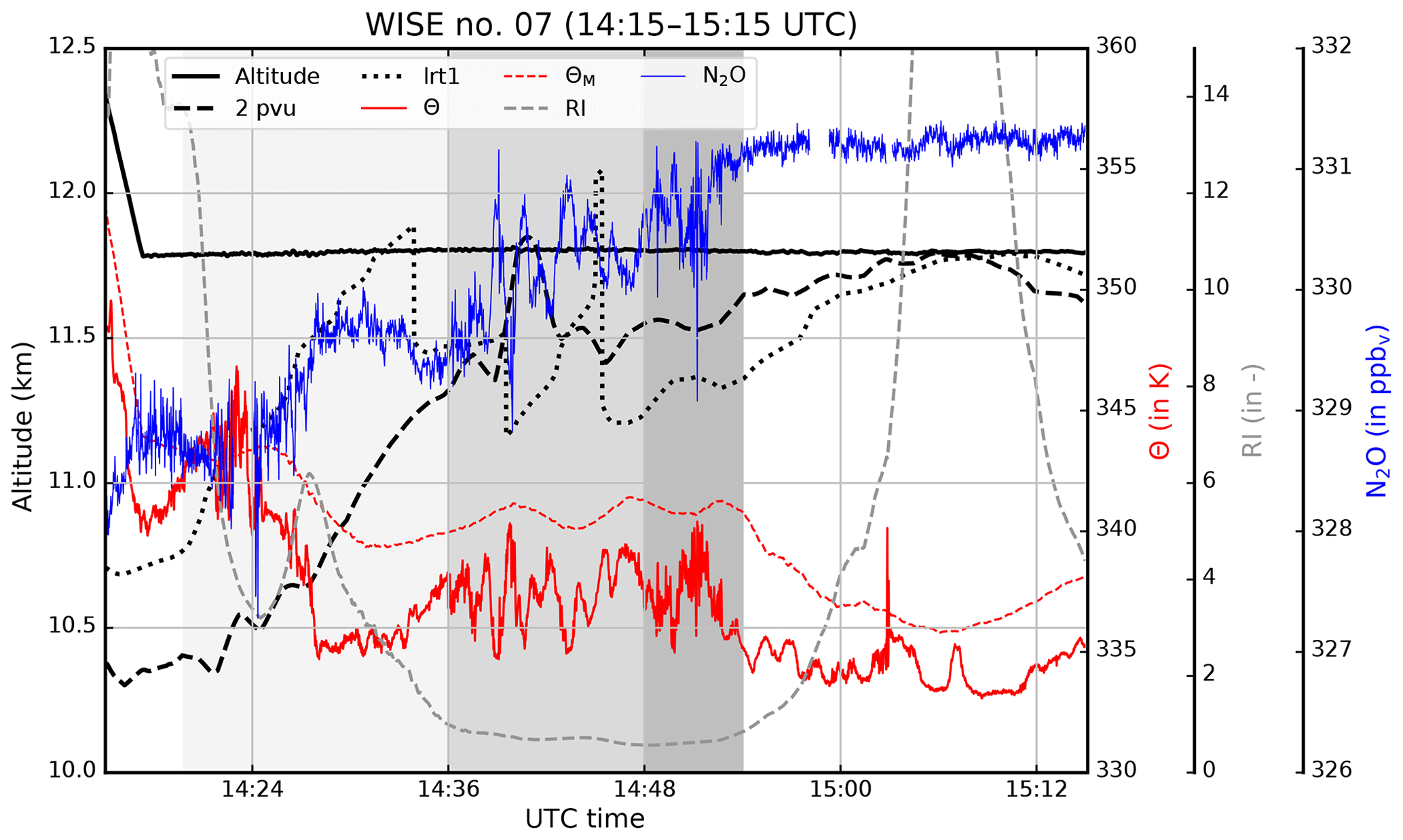
Figure 4Time series of measured N2O (blue) and potential temperature Θ (red solid) as well as modeled potential temperature ΘM (red dashed), Richardson number Ri (gray dashed), and altitudes of the dynamic (2 pvu, black dashed) and the first lapse rate (lrt1, black dotted) tropopause between 14:15 and 15:15 UTC during WISE RF07. Black solid line shows the altitude of the aircraft, the gray areas indicate the time periods discussed in the text.
Now we focus on the flight leg from northeast to southwest at FL380 between 14:20 and 15:20 UTC. HALO came from FL400 which was then deeper in the stratosphere with potential temperatures above 350 K. At FL380 HALO was initially flying in the lowermost stratosphere, then gradually approaching and finally crossing the dynamic tropopause, which was slightly tilted according to the ECMWF analysis (Fig. 3a). This is in remarkable agreement with measurements of N2O, which increases to tropospheric values at FL380 (Fig. 4), as is discussed further below. On this leg the aircraft crossed the lower part of the structures with alternating large and low values of static stability. This structure is potentially linked to a propagating inertia-gravity wave which commonly emerges during baroclinic wave developments (e.g., O'Sullivan and Dunkerton, 1995). Furthermore, in the region with low values of static stability an area with low Richardson numbers is evident which extends into the region of the maximum of static stability at around 15:00 UTC.
Before we analyze the time period between 14:00 and 15:00 UTC more specifically in Sect. 3.2, we want to point out one model deficiency. Although the ECMWF forecast predicted the atmospheric state very well, there is evidence that extreme values of state parameters are missed or at least underestimated, with potential consequences for the representation of mixing in the UTLS. We already mentioned that we think that the Richardson numbers from the ECMWF forecast might have values that are too large in regions around the tropopause where the vertical shear of the horizontal wind is large. However, this is difficult to verify from airborne measurements, since all two-dimensional information on the temperature and wind is missing along the flight path. We can overcome this issue at least partly by using temperature retrievals from GLORIA and comparing static stability (the numerator of the Richardson number calculation) from the model and from measurements (Fig. 3b, c). For this we use the last northeastward leg on FL420, i.e., ∼ 13 km and 169 hPa, between 17:20 and 18:20 UTC, when HALO was flying above the maximum values of static stability. Static stability from GLORIA measurements exhibits larger values than that from the ECMWF model as well as a smaller vertical extension of the entire wave structure. Thus, the model forecast underestimates the strength of the inversion, most potentially related to deficiencies in representing the gravity wave in this region due to the still relatively coarse grid spacing in the UTLS. Since the gravity wave also affects the three-dimensional wind, it could be assumed that the vertical shear of the horizontal wind might not be sufficiently represented in the model and thus the gradient Richardson number.
In summary, the synoptic situation during WISE RF07 strongly resembles the situation of the idealized baroclinic wave of Kunkel et al. (2016). Consequently, it is now possible to investigate a prediction from an idealized model study with airborne measurements and seek signs of turbulent motions in the measurement data.
3.2 Airborne in situ measurements and evidence of mixing around the tropopause – WISE RF07
We start our analysis by focusing on the time period between 14:20 and 14:54 UTC (gray areas in Fig. 4) and will first concentrate on the in situ measurements of nitrous oxide N2O and potential temperature Θ along with several parameters from the ECMWF forecast interpolated on the flight track. Based on N2O and Θ we further subdivided the time period of interest into three shorter periods (gray scales in Fig. 4). During the first period from 14:20 to 14:46 UTC, N2O volume mixing ratios below 331.31±0.45 ppbv indicate that HALO was flying in an air mass of stratospheric origin. This value represents the airborne measured tropospheric mean of N2O during the WISE campaign and is calculated following Müller et al. (2015). HALO was flying at a constant pressure level while slowly approaching the dynamic as well as the first lapse rate tropopause. In the second time period between 14:36 and 14:48 UTC the distance between tropopause and flight level decreased to a few hundred meters or less according to the PV analysis. Notably, this part of the flight close to the tropopause in the ExTL shows low Richardson numbers. Around 14:40 UTC the time series of both N2O and Θ show strong wave-like structures with periods of about 2 min. The horizontal wavelength can be roughly estimated to be about 25 km, using a mean ground speed of 210 m s−1 of HALO during this part of the flight and assuming that the wave has been crossed perpendicular to the wave crests. The amplitude of the wave is about 2.5 K and the wave spans the potential temperature range between 335 and 340 K. Interestingly, this wave structure is hardly evident in the modeled ΘM, indicating that the model might have issues representing these scales accurately. The model shows signs of gravity wave activity, however, not directly at the flight altitude but slightly above (not shown). The ECMWF forecast model with a horizontal grid spacing of about 8 km can barely resolve this wave pattern with this fine-scale structure due to the grid spacing of the model. The last period between 14:48 and 14:54 UTC shows strong variability in both N2O and Θ without any clear wave signal but large variability of Θ and N2O. This increase in variability could be regarded as a first indicator of increased atmospheric turbulence.
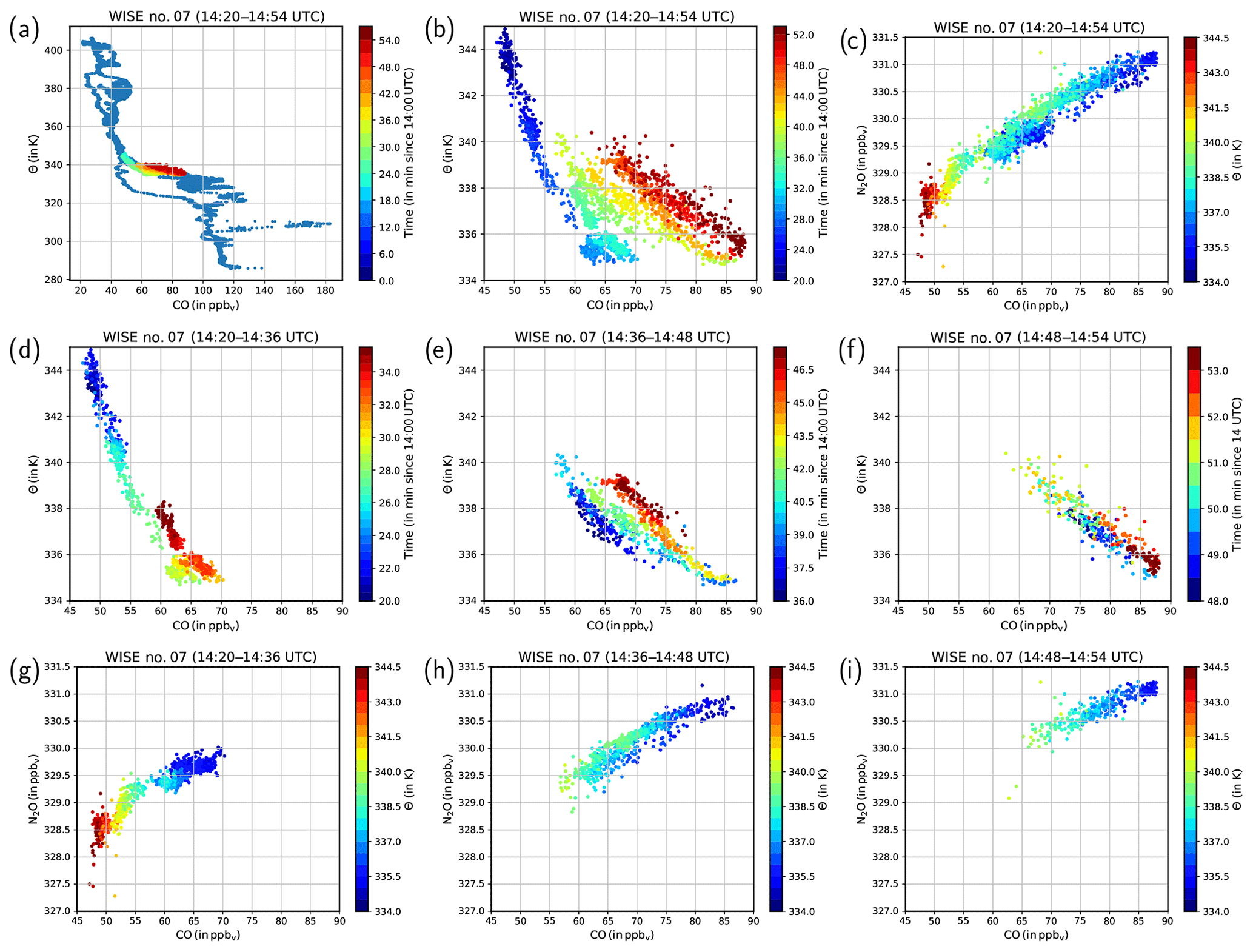
Figure 5Trace gas analysis of the first southwestward leg on FL380, i.e., 205 hPa of WISE RF07. (a) Vertical profile of carbon monoxide for the entire flight (blue dots) and color-coded for the leg on FL380. (b) Vertical profile of CO for the time period 14:20–15:00 UTC, color-coded with time since 14:00 UTC. (c) CO–N2O correlation for the time period 14:20–15:00 UTC, color-coded with potential temperature. (d–f) Vertical profiles of CO for time periods 14:20–14:36, 14:36–14:48, and 14:48–14:54 UTC, color-coded with time. (g–i) CO–N2O correlations for the time periods 14:20–14:36, 14:36–14:48, and 14:48–14:54 UTC, color-coded with potential temperature.
If turbulence occurred in a region of strong tracer gradients at or upwind of where the measurements were taken, it should have affected the composition of trace gases. Both CO and N2O exhibit vertical gradients in the lower stratosphere (Fig. 5a for CO). We first focus on CO since it has a much stronger gradient at the tropopause due to its shorter lifetime compared to N2O. HALO was initially in the stratosphere with low values of CO and at the end of the time period close to the troposphere with larger values of CO (Fig. 5b). The gradual transition between the more stratospheric to more tropospheric CO values occurs at potential temperatures between 335 and 340 K. This Θ interval also shows low Richardson numbers in the ECMWF model (Figs. 4, 3a). Moreover, the color code in Fig. 5b reveals the consecutive alternation between low potential temperature/large CO values and high potential temperature/low CO values, indicating the impact of the small-scale wave on the tracer and potential temperature. To identify mixing of tracers, we analyzed the N2O–CO relationship, which provides information on irreversible tracer exchange similar to CO–O3 (e.g., Fischer et al., 2000). In general, at the tropopause the CO–N2O correlation shows almost tropospheric mixing ratios of CO (∼90 ppbv) and N2O (∼331 ppbv) at potential temperature levels typical for the extratropical tropopause in the current case (∼335 K). Above the tropopause both N2O and CO mixing ratios decrease with increasing potential temperature. However, the CO–N2O correlation of the time period between 14:20 and 14:54 UTC does not show such a clear relationship of decreasing N2O and CO and simultaneously increasing potential temperature (Fig. 5c). If the time period is instead divided into three shorter time periods following the gray shading in Fig. 4, then only the first period shows a relationship between N2O, CO, and potential temperature as one would expect from the large-scale vertical profiles of these quantities (Fig. 5d, g). However, for the other two time periods the tracer–tracer relation with respect to potential temperature changes. For the time between 14:36 and 14:48 UTC the vertical profile of CO shows a wave-like transition (Fig. 5e), while the correlation shows isentropic mixing on different isentropes as indicated by mixing lines connecting tropospheric and stratospheric values between 335 and 340 K (Fig. 5h). In the last time period the relation between N2O, CO, and potential temperature seems to almost entirely break down, reflecting the initial thought of increased variability in the tracer mixing ratio and potential temperature (Fig. 5f, i). Thus, based on the trace gas analysis, we think that turbulence increasingly affected the second and third time periods to a substantial degree in contrast to the first time period. This could ultimately lead to exchange of trace constituents across the tropopause in a narrow range of potential temperature levels.
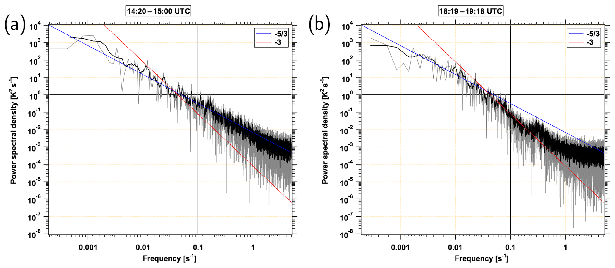
Figure 6Power spectral densities of measured potential temperature from HALO for selected time periods: (a) 14:20–15:00 UTC and (b) 18:19–19:18 UTC. Black solid lines are introduced for better comparability, red solid line shows a line with a slope of , blue solid line shows a line with a slope of .
We further analyze the occurrence of turbulence with the help of power spectral densities of potential temperature. Power spectral densities of trace species or state parameters allows the estimation of how much energy is present at a particular spatial scale (Vallis, 2017). On board HALO the frequency of measurements is about 10 Hz for the state parameters such as temperature and wind, while it is about 2–3 Hz for CO and N2O. Along with an average ground speed of about 210 m s−1 and with the 10 Hz measurements of the state parameters this potentially allows us to identify atmospheric structures down to about 100 m. The shape of these power spectral densities allows the contribution of individual scale ranges to the total energy spectrum to be assessed and indicates the type of turbulence that affects the considered domain (Vallis, 2017). The power spectral density from the flight leg on FL380 (Fig. 6a) reveals a slope close to . This slope often characterizes three-dimensional isotropic turbulence, i.e., dynamic processes on or below the mesoscale affect the flow (e.g., Tung and Orlando, 2003; F. Zhang et al., 2015). At a later leg in the same direction of the flight on flight level FL420 between 17:20 and 18:20 UTC the power spectral density follows a slope of (Fig. 6b). This slope indicates a dominance of geostrophic turbulence and thus larger synoptic scales affecting the flow. To summarize, the slope of close to the tropopause suggests that mesoscale processes, e.g., those related to gravity waves, might be substantial to explain the dynamics in the tropopause region.
3.3 Trajectory-based history of measured air masses during WISE RF07
The analyses of trace gas distributions, tracer–tracer correlations, and power spectral densities suggest that mixing is evident in the region between 335 and 340 K. In particular, the N2O mixing ratios reveal that tropospheric and stratospheric air masses participate in the mixing process. Our next goal is to elucidate the recent history of the measured air masses. For this we calculated kinematic trajectories backward and forward in time which start each second along the flight path for the time period between 14:24 and 14:54 UTC based on ECMWF forecast data available between 28 September 2017 at 00:00 UTC and 29 September 2017 at 12:00 UTC. More specifically, the trajectories start at the horizontal location of the airplane as well as at adjacent locations in longitudinal and latitudinal directions to cover some of the uncertainty due to the gridded representation of the meteorological input variables and to increase the number of trajectories for statistical purposes. Moreover, trajectories start at each full isentropic level between 334 and 341 K and not only at the flight altitude of HALO. This allows us to study the fate of the entire region, which is subject to mixing according to the measurement.
Since we are interested in STE and mixing, we first search for those air masses which cross the tropopause around the time of the measurement and which encounter a KHI. For this we filter all trajectories to find those trajectories which cross the dynamic tropopause and which encounter Richardson numbers smaller than 1 at any point in time during the period of the trajectory calculation. We note, however, that our STE criterion is rather weak, since we only require that the PV of the trajectories is below the PV threshold for the dynamic tropopause at the start of the analysis (28 September 2017 01:00 UTC) and above the threshold at the end (29 September 2017 11:00 UTC). Thus, for further discussion we omit the terminology of TST and STT trajectories as coherent ensembles of trajectories which cross the tropopause only once from the troposphere (stratosphere) to the stratosphere (troposphere) (Stohl et al., 2003; Wernli and Davies, 1997). We think instead of trajectories which show the potential of mixing around the tropopause by encountering low Richardson numbers and having PV values changing between tropospheric and stratospheric values, which nevertheless lead to a subsequent exchange across the tropopause. As mentioned above, we consider low Richardson numbers of the order of 1 as good proxies for KHI. We further study the three time periods of interest from the earlier analysis separately (Fig. 4).
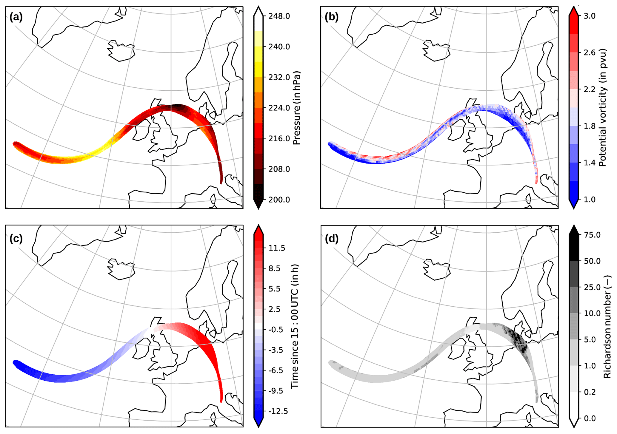
Figure 7Trajectories crossing the 2 pvu isosurface and encountering a dynamic instability which cross the flight track between 14:36 and 14:48 UTC while HALO was flying on FL380. Trajectories start on 28 September 2017 at 01:00 UTC and end on 29 September 2017 at 11:00 UTC. The four panels show the following quantities along the trajectories: (a) pressure (in hPa), (b) potential vorticity (in pvu), (c) time since 15:00 UTC (in h), and (d) Richardson number. In total each panel shows 12 375 individual trajectories.
Interestingly, we find trajectories indicating upward transport which show the same behavior in dynamic and thermodynamic quantities in each of the three time periods between 14:20 and 14:54 UTC. These trajectories always follow a wave-like flow from the North Atlantic towards the British Isles before they turn anticyclonically towards central Europe (Fig. 7). Minimum pressure is evident over the North Atlantic when the trajectories pass through the large-scale trough. Over Ireland and the British Islands the trajectories rise again while encountering the region of the KHI with minimum Richardson numbers. Starting from this region the trajectories strongly decelerate (see Fig. 7c) in a region of alternating horizontal divergence (not shown explicitly).
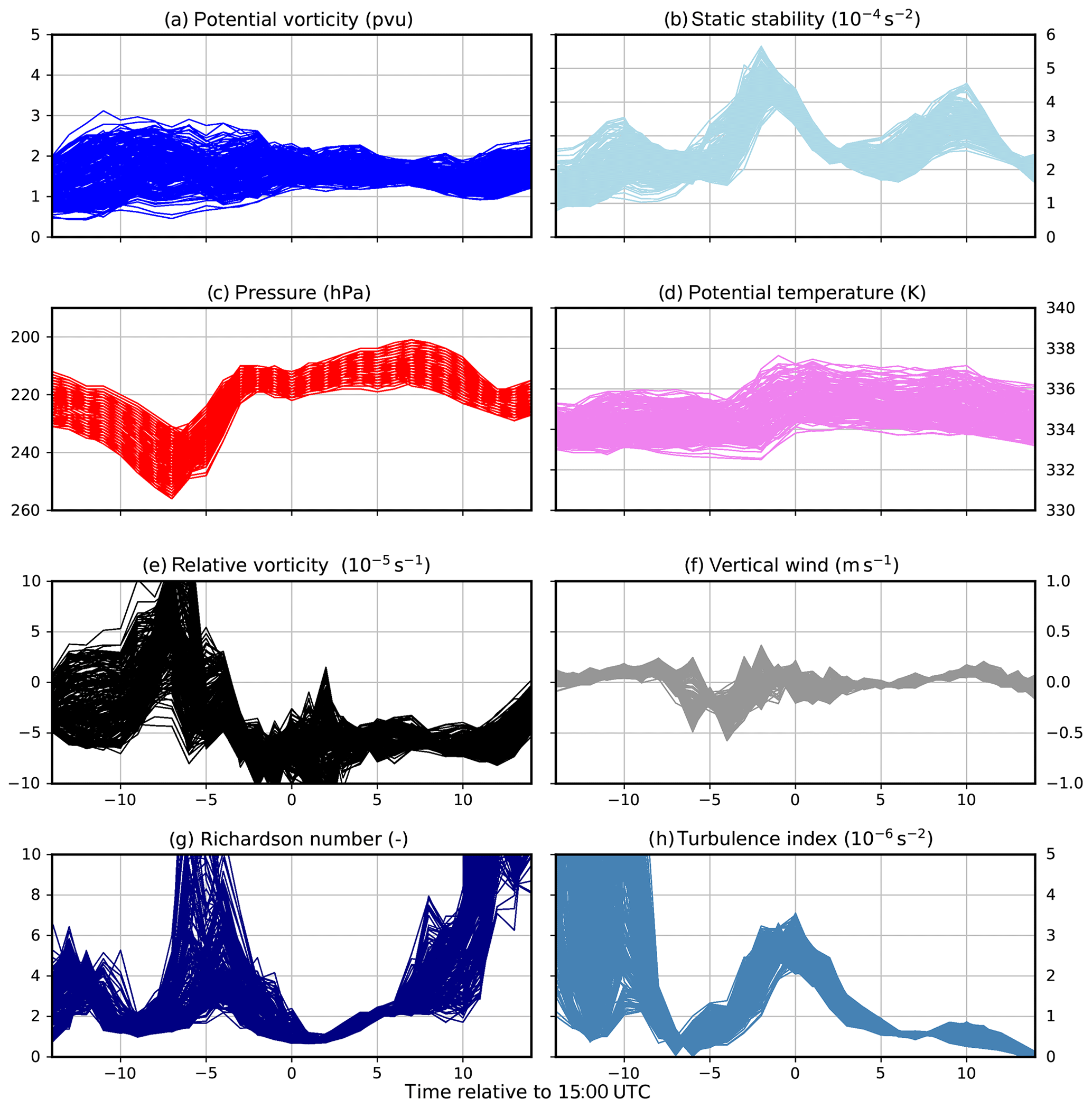
Figure 8Time series of dynamic and thermodynamic quantities of mixing trajectories crossing the dynamic tropopause and experiencing a KHI. The time axis is relative to 28 September 2017 at 15:00 UTC. The eight panels show the following variables along the trajectories: (a) potential vorticity (in pvu), (b) static stability (in 10−4 s−2), (c) pressure (in hPa), (d) potential temperature (in K), (e) relative vorticity (in 10−5 s−1), (f) vertical wind (in m s−1), (g) Richardson number, and (h) turbulence index after Ellrod et al. (1992) (in 10−6 s−1). Note that the time period shown here is shorter than the total time period used for the trajectory analysis.
The analysis of the PV along the potential TST trajectories shows that these trajectories oscillate around the dynamic tropopause rather than cross the tropopause as a coherent ensemble once and then reside in the lower stratosphere. This is somewhat evident in Fig. 8a, where only those trajectories are shown which at the physical start time of the trajectories have PV values initially smaller and at the last physical time step have PV values larger than the respective dynamic tropopause PV value (here 2 pvu). The trajectories show no straight traverse from the troposphere into the stratosphere. However, several points shall be noted for the time close to the measurement briefly before 15:00 UTC. The static stability shows a maximum which is not evident in PV but is accompanied by a strong decrease in relative vorticity towards anticyclonic flow (Fig. 8b, e). The maximum in static stability follows a period where the trajectories encounter alternating vertical wind, which is a sign of flow through small-scale waves. At the end of this time period signs of turbulent motions increase. Initially, the turbulence index increases due to vertical wind shear as well as stretching and shearing deformation (Ellrod et al., 1992). Later low values of the Richardson number emerge which are indicative for KHI. The appearance of turbulence is further associated with a slight increase in potential temperature which is on the order of 1–2 K, thus the process can be regarded as quasi-isentropic.
The major difference between the three time periods between 14:20 and 14:54 UTC is the number of occurrences of these characteristic mixing trajectories, relative to the dynamic tropopause. During the first part between 14:20 and 14:36 UTC, we find only about 1.7 % out of 69 048 trajectories crossing the tropopause and having low Richardson numbers. This number increases to 23.9 % out of 51 768 in the second part and to 21.9 % out of 25 920 in the last part from 14:48 to 14:54 UTC. Notably, this result does not depend on the choice of our PV value for the dynamic tropopause. This indicates that a rather thick layer around the tropopause up to 3.5 pvu is affected by this mixing process, in particular between 14:36 and 14:48 UTC according to the trajectory analysis. Moreover, there is also a tendency of air masses from above to be mixed downward. For this we select trajectories which initially have a PV value above and finally below the desired dynamic tropopause value. Although they are most evident in the second and third part, such trajectories are in general much less common than those with an increasing PV value over the considered time period. In line with this is that the stratospheric influence on the measured air masses substantially decreases from the first to the third time period. While about two-thirds of the trajectories originate in regions above 5 pvu in the first part, only about a quarter does in the second part and less than 0.5 % in the third part.
Consequently, the trajectory analysis shows that different air masses of tropospheric and stratospheric origin come together in the second and third part of the considered time period. This is in line with the measured trace gas concentrations of N2O and CO. However, based on the trajectory analysis it is difficult to estimate whether STE and in particular TST occurs in a way that air parcels cross the dynamic tropopause only once from the troposphere into the stratosphere and stay there afterwards. We also performed longer trajectory calculations which, however, also provide no further evidence of TST trajectories which then reside in the stratosphere over a longer time period. We instead find trajectories which, based on PV, alternate back and forth between troposphere and stratosphere and which encounter low Richardson numbers along their paths. One potential reason for why no TST trajectories which stay in the stratosphere are found is that the model fails to correctly resolve the process. In contrast, assuming that the model performed well, it could simply mean that in this specific case the mixing occurred only across the tropopause with no substantial STE taking place. Independently of which is the case, this process changes the gradients of the trace gases in this region which in turn is of importance for radiative transfer calculations (e.g., Riese et al., 2012).
After the analysis of airborne measurements, the first question to arise is how generic such a mixing process may be in ridges of baroclinic waves. We can answer this question at least partly when searching for this process in idealized baroclinic life cycle experiments which are generic counterparts of atmospheric baroclinic waves. If the process is evident in the experiments, it might occur frequently in the real atmosphere and thus be of significance. Furthermore, the idealized experiments allow us to further analyze the physical processes which lead to mixing and potentially to STE. For this we use model results based on the idealized simulations already used in Kunkel et al. (2016). The simulations include non-conservative processes (in terms of PV) such as large-scale and convective cloud microphysics, radiative effects from trace species and clouds, and vertical turbulence. These simulations were labeled with BRTC (bulk microphysics, radiation, turbulence, and convection) in Kunkel et al. (2016). We further conducted simulations for life cycles 1 and 2 (Thorncroft et al., 1993); however, we focus our discussion here on results for life cycle 1. We extended the BRTC simulations by including tracers to mark the air which was initially in the stratosphere or troposphere as well as to trace the initial PV distribution. Furthermore, we calculated kinematic trajectories to analyze STE.
We first show that STE occurs in the model simulation. For this we calculated backward trajectories starting every 6 h between 24 and 192 h of model integration. The start points of these trajectories were distributed around the dynamic tropopause, i.e., the 2 pvu isosurface. They were initialized at each grid point in the horizontal and between 1.5 km below and 1.5 km above the local dynamic tropopause in the vertical. Each time, more than 240 000 trajectories are then traced back for 6 h and consequently filtered based on whether they cross the tropopause. Furthermore, we searched for those STE trajectories which change their potential vorticity within the 6 h by a given PV value to circumvent a residence time criterion suggested by Wernli and Bourqui (2002). For instance, we assume that trajectories which have an initial potential vorticity smaller than 1.5 pvu and a final one of larger than 2.5 pvu have a larger probability of staying in the stratosphere than if the only criterion is to cross the 2 pvu isosurface.

Figure 9Temporal evolution of maximum static stability (black, in 10−4 s−2), minimum surface pressure (red, in hPa) as well as the number of TST and STT trajectories per 6 h interval over the course of the idealized baroclinic life cycle experiment BRTC LC1. The maximum static stability is derived by first averaging the static stability in the vertical between the altitudes of the local lapse rate tropopause and 1 km above. The maximum value is then determined from the resulting two-dimensional field over the horizontal model domain.
The number of TST and STT trajectories based on these 6 h long back trajectories reveal that STE starts to occur slightly after the time of the first enhancement of N2 during the growing stage of the surface cyclone (Fig. 9). Kunkel et al. (2016) attributed the increase in lower stratospheric static stability to updrafts in the troposphere. This can be regarded as the first time step when the tropopause is affected significantly by the tropospheric dynamics related to the baroclinic wave. Note that the initial state of the baroclinic life cycle experiments is designed such that the tropospheric background value is s−2 and that the stratospheric value is s−2. Peak values for STE are evident after 160 h of model integration, in the final stage of the life cycle (Reutter et al., 2015).
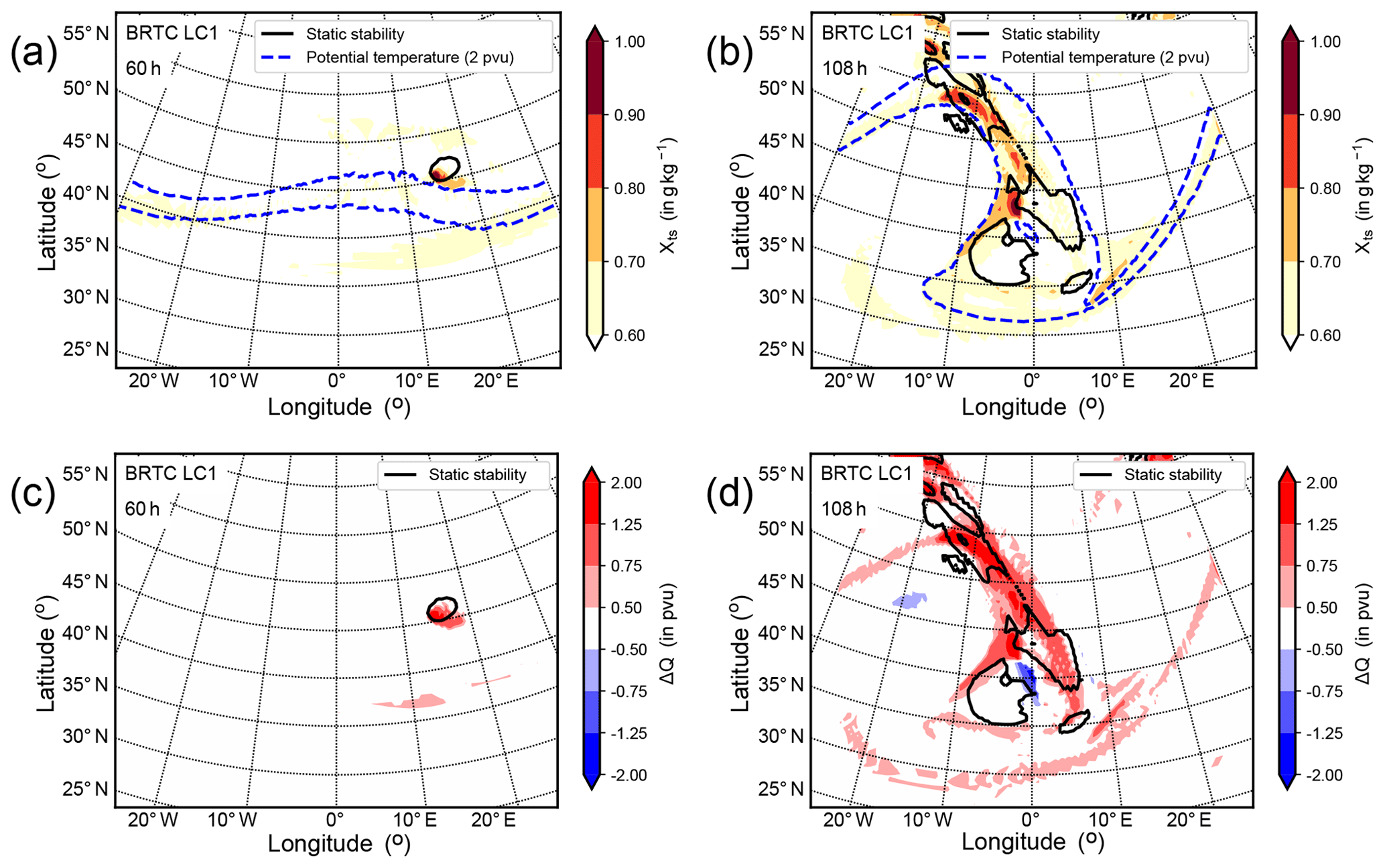
Figure 10The tropospheric tracer Xts on first full stratospheric level, i.e., the first full level with PV values larger than 2 pvu for (a) 60 h and (b) 108 h after model start. Diabatic change of PV, , at the level of the dynamic tropopause with Q0,adv being the advected initial PV and Q being the full PV for (c) 60 h and (d) 108 h after model start. The black isoline shows static stability, s−2. The blue dashed lines show isolines of potential temperature for 315 and 325 K.
We also find a spatial coincidence in the horizontal plane between the enhancement of N2 above the thermal tropopause and TST across the dynamic tropopause by analyzing passive tracers in our idealized simulations (Fig. 10). The tropospheric tracer, initialized with a constant non-zero mixing ratio in the troposphere and zero in the stratosphere, shows enhanced values at the first model layer in the stratosphere, exactly in the region where static stability is also enhanced. We define the first model level in the stratosphere as the first full model level above the dynamic tropopause. This region also marks the region where the tropospheric tracer enters the stratosphere. This is first evident after about 60 h (Fig. 10a), but also at later time steps (Fig. 10b). We can further confirm these findings based on our diabatic PV tracer. This tracer carries the information about the difference between the current and the initial value of PV in each grid box (Kunkel et al., 2014). Evaluating this difference in the dynamic tropopause allows us to diagnose whether an air mass at the dynamic tropopause gained or lost PV, and thus whether this air mass initially resided in the troposphere or in the stratosphere. Positive values of this difference indicate a gain of PV, i.e., TST, and negative values a loss of PV, i.e., STT, of the respective air mass at the dynamic tropopause since model start (Fig. 10c, d). In contrast to TST and although a temporal coincidence is also evident for N2 enhancement and occurrence of STT, no spatial co-occurrence is evident for STT in regions of enhanced N2 (Fig. 10c, d; and also based on the analysis of the stratospheric tracer which is not shown explicitly here). Thus, from the distribution of these passive tracers, we can conclude that there is also a spatial coincidence between TST and enhancement of static stability.
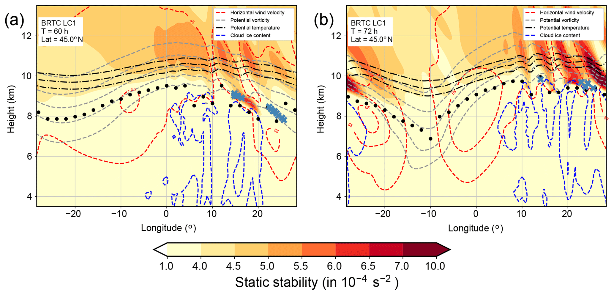
Figure 11Zonal cross sections along the center of the model domain at 45∘ N show static stability (contour filled), potential temperature (330, 335, 340 K, black lines), cloud ice water content ( kg kg−1, blue lines), potential vorticity (2–6 pvu, gray lines), and the altitude of the thermal tropopause (black dots). Red lines show isolines of the horizontal wind speed (45–65 m s−1) and blue crosses show points of trajectories at the respective longitude which cross the tropopause from the troposphere to the stratosphere over the course of the last 6 h for (a) 60 h and (b) 72 h after model start.
Furthermore, the exchange occurs in the ridge of the baroclinic wave, just above a region of ice cloud occurrence (Fig. 11). This region is also strongly affected by a small-scale wave pattern related to a propagating inertia gravity wave which is evident in the isolines of potential temperature and PV. This wave is one source of the enhanced values of static stability. The other source is radiative cooling below and at the tropopause related to ice clouds in the upper troposphere. The first time TST occurs in this region is after about 60 h, while it is evidently more frequent during later stages of the life cycle. We thus find a pathway from the troposphere into the stratosphere in the ridge of baroclinic waves in our idealized simulations. The situation is as initially expected from the results of Kunkel et al. (2016) and resembles the situation of the mixing and potential TST in the ridge during WISE RF07.

Figure 12Trajectories starting 66 h and ending 72 h after model start which increase their PV from values smaller than 1.5 pvu to values larger than 2.5 pvu within the 6 h interval. Panels show (a) static stability (in 10−4 s−2), (b) potential temperature (in K), (c) relative vorticity (in 10−5 s−1), and turbulent kinetic energy (in m2 s−2) along the trajectories for each hour.
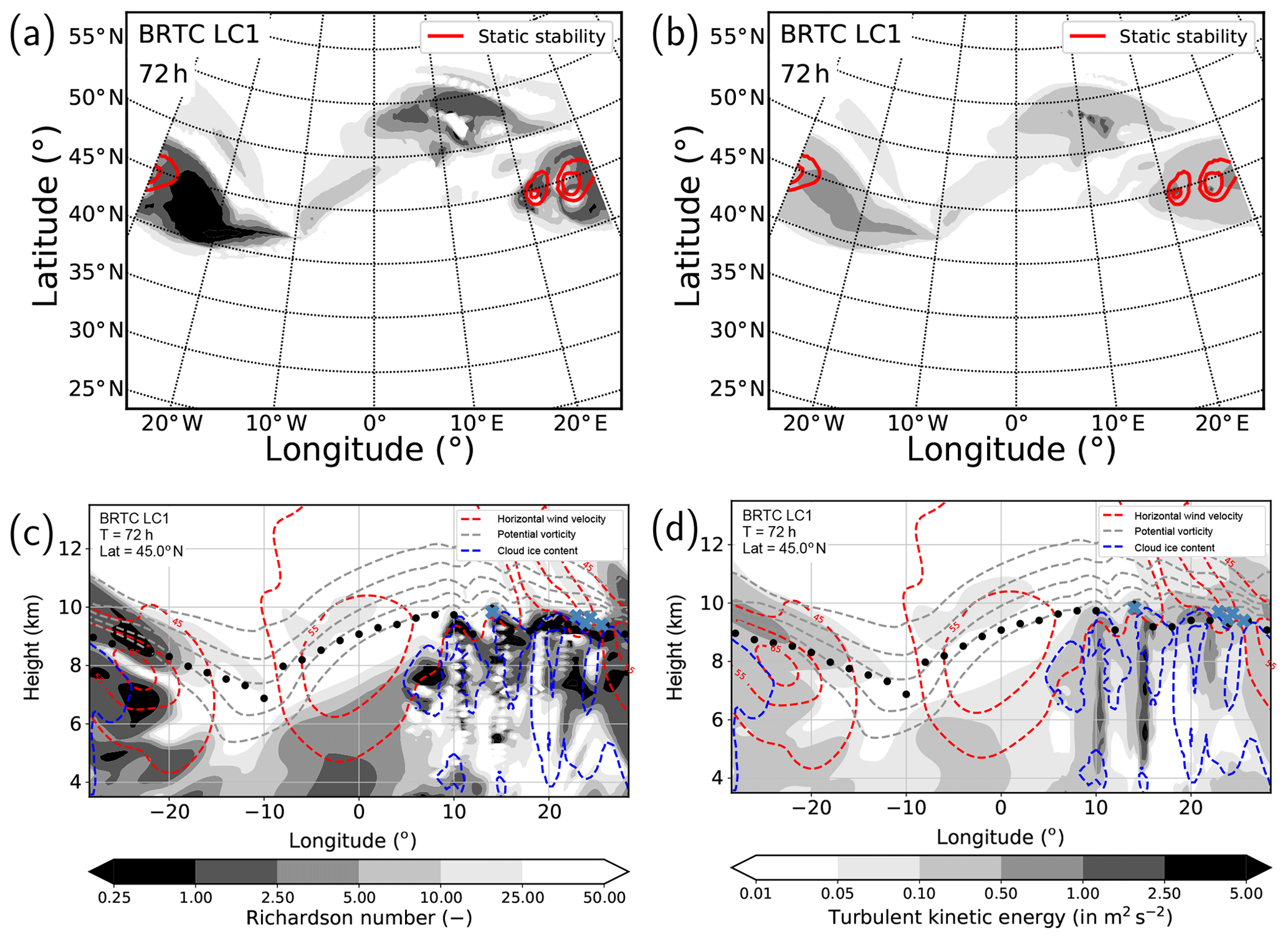
Figure 13Panels (a) and (c) show gradient Richardson number, Ri, panels (b) and (d) TKE after 72 h of model integration. Panels (a) and (b) show a horizontal cross section at the dynamic tropopause along with isolines of static stability with values of s−2 and s−2; panels (c) and (d) show zonal cross sections at 45∘ N in the center of the model domain, including isolines of various variables (see detailed description in Fig. 11).
Before we end our discussion by studying the processes leading to mixing, we want to highlight the fact that in our idealized simulations two types of TST trajectories are apparent (Fig. 12). One set of TST trajectories exhibits low values of static stability, low potential temperatures, positive relative vorticity, and moderate turbulent kinetic energy (TKE). In contrast, the other set of TST trajectories shows large values of static stability, higher potential temperatures, negative relative vorticity, and larger values of TKE. Thus, while the first set of trajectories crosses the tropopause at the cyclonic side of the jet at rather low altitudes, the other set of trajectories crosses the tropopause at the anticyclonic side of the jet at rather high altitudes. Such trajectories are found over a large part of the life cycle and also in the case where we apply different criteria for a change of PV, e.g., from 1.5 to 3.0 pvu. A common feature of the two sets of trajectories is that in both cases the potential temperature values hardly change in the 6 h; thus, the TST occurs quasi-isentropically. We also note that the trajectories crossing the tropopause in the ridge of the wave experience large values of static stability, thus passing through the TIL. Thus, what initially might seem counter-intuitive, i.e., the exchange in the vicinity of large values of static stability inhibiting vertical motions, is nevertheless possible in the ridge of the baroclinic waves.
The last point that we want to address is the processes causing the mixing and exchange across the tropopause in the ridge of the baroclinic wave. The occurrence of turbulence becomes apparent from low values of the gradient Richardson number and enhanced values of TKE (Fig. 13). The Richardson number is the ratio between static stability and vertical shear of the horizontal wind. Since static stability shows rather large values above the tropopause, the source of low Richardson numbers results from large vertical shear of the horizontal wind (Fig. 14a). The shear is largest in the ridge where a gravity wave is evident at the edges of the jet stream. The shear also contributes to enhanced values of TKE and might thus explain its enhancement. However, TKE further depends on the vertical gradient of the total moisture, which can consequently lead to a buoyant heat flux (Doms, 2011). This buoyant heat flux shows positive and negative values at the tropopause, most probably related to the propagating and potentially dissipating gravity wave (Fig. 14b). In particular, in the region of the TST trajectories negative values are dominant which could indicate upward motions in an otherwise stable environment. The stability is further increased by a radiative feedback of the ice clouds (Fig. 14c). Cooling is evident at the top of the clouds which in turn enhances the static stability above the tropopause in the region of the mixing (e.g., Fusina and Spichtinger, 2010; Kunkel et al., 2016). Thus, we identified the processes which allow for mixing induced by shear in a region which is stably stratified.

A recent study by Kunkel et al. (2016) showed the concurrent occurrence of enhanced static stability in the lower stratosphere and increased turbulent motions across the extratropical tropopause in the ridge of idealized baroclinic life cycles. Here, we present evidence that such a situation corresponds with mixing of trace gases at the level of or slightly above the tropopause and eventually with transport of tropospheric air into the stratosphere. To the authors' knowledge this process has gained only a small amount attention so far, in particular in terms of the formation of the extratropical transition layer. We derive our conclusions from airborne measurements along with high resolution ECMWF model data to identify the occurrence of mixing and potential TST in the ridge of a baroclinic wave. We further extended experiments of idealized baroclinic life cycles from Kunkel et al. (2016) to elucidate the driving mechanisms and to obtain a more general picture of the mixing process.
During WISE RF07 signs of turbulent mixing are evident between 335 and 340 K potential temperature in the lowermost stratosphere just above the tropopause. The region of interest was situated above an extended cloud deck associated with a warm conveyor belt outflow and was substantially affected by small-scale waves in the lowermost stratosphere. Vertical profiles of tracers with a sufficient long lifetime in the UTLS such as CO and N2O and their correlations are used to identify quasi-isentropic mixing between air masses of different origin. In particular, the N2O tracer mixing ratios suggest that tropospheric and stratospheric air masses mix in this region. Power spectral densities of potential temperature support the analysis suggesting that mesoscale rather than synoptic-scale processes affect the power spectrum in the region of mixing.
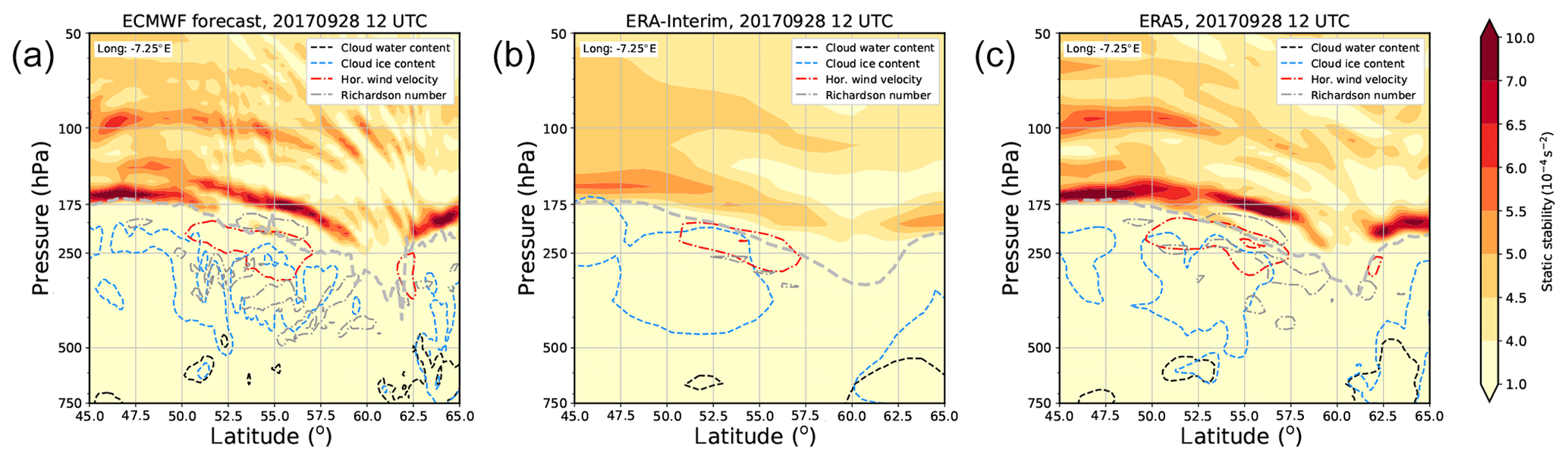
Figure 15Zonal cross sections along −7.25∘ E on 28 September 2017 at 12:00 UTC show static stability (color shaded), the altitude of the 2 pvu isosurface (light gray), cloud water content (black), cloud ice content (blue), horizontal wind speed (red), and Richardson number (dark gray). The three panels show (a) the ECMWF forecast (with 0.07∘ horizontal grid spacing and ∼300 m vertical grid point spacing in the UTLS), (b) the ERA-Interim reanalysis (with 0.75∘ horizontal grid spacing and ∼1000 m vertical grid spacing), and (c) the ERA5 reanalysis (with 0.25∘ horizontal grid spacing and ∼300 m vertical grid spacing).
Furthermore, ECMWF forecast data with the highest available resolution are used to obtain a broader view on the synoptic situation. Although the model performs well in representing the overall situation, some deviations have been found between model and measurements. In particular, these deviations occur at small scales which seem to be substantial in the representation of the mixing process. Nevertheless, trajectory calculations based on the model data show that mixing occurs around the tropopause and affects the lower part of the extratropical transition layer. The mixing occurs in regions of enhanced lower stratospheric static stability, relatively high potential temperature, anticyclonic flow, and during a time when the flow is affected by vertical shear, deformation, and moderate alternating vertical motions.
Moreover, numerical experiments of idealized baroclinic life cycles support the observational findings. In the model simulations it is evident that mixing occurs in the ridge of baroclinic waves, just above the top of ice clouds. Using special tracers and kinematic trajectories, we showed that even TST occurs in regions of enhanced static stability, thus in the region of the TIL. To a large degree the mixing is the result of a Kelvin–Helmholtz instability which has its source in enhanced vertical shear, as has recently been demonstrated by Kaluza et al. (2019). This shear is strongly related to inertia-gravity wave dynamics at the upper edge of the jet stream. Moreover, buoyant heat fluxes caused by the upper-tropospheric clouds may also enhance the turbulence across the tropopause.
The overall relevance of this process still needs to be analyzed. This is beyond the scope of the current study. However, on the one hand this process occurs on small scales, and is related to cirrus clouds at the tropopause and a strong wind shear which in turn seems to be related to small-scale waves in the lower stratosphere. Thus, the impact on the trace gases in the upper troposphere and lower stratosphere might be not particularly large due to the limited geographical extent of the combinations of these processes. On the other hand all this occurs within baroclinic life cycles which are relatively frequent features of the extratropical UTLS. Thus, there is potentially a non-negligible contribution of this mixing process to the composition of the extratropical transition layer. In particular, since this mixing occurs at relatively high potential temperatures, it can affect regions which have previously not been considered to be strongly affected by STE in baroclinic waves. Previous studies showed that the main exchange in the extratropics occurs at lower potential temperature levels at the lower edge of the jet stream.
One reason why the process described in this study has not gained much attention is that numerical weather prediction models and in particular reanalysis products as well as climate models do not resolve the UTLS sufficiently, thus potentially missing or misrepresenting the relevant processes. However, reanalysis data sets in particular build the basis for almost all recent climatological studies of STE (e.g., Škerlak et al., 2014; Boothe and Homeyer, 2017). Figure 15 shows the same cross section for different ECMWF products. While the forecast shows many fine-scale features, e.g., in the cloud structure and the location of the tropopause, these features are almost entirely missing in ERA-Interim. This is to a large degree caused by the poorer vertical resolution of ERA-Interim, which is similar to the resolution in current climate models. In contrast, the new ERA5 reanalysis data which use the same vertical grid spacing as the current forecast model show more similarity to the forecast and might thus allow for a better representation of STE in the extratropics than ERA-Interim. However, potentially even the forecast data still have problems capturing all features fully and correctly, because the vertical grid spacing of that data is still relatively coarse compared to our idealized simulations with a vertical grid spacing of 110 m and a horizontal grid spacing of 0.4∘, which captured the TST relatively well. Thus, an increase in vertical model resolution seems to be necessary to further address this process and its potential consequences, on smaller as well as larger scales.
ECMWF (forecast, ERA-Interim, and ERA5) data have been retrieved from the MARS server. The airborne measurement data from the WISE campaign are available through the HALO database (https://halo-db.pa.op.dlr.de/, last access: 1 October 2019). The code of the COSMO model is available on request from the COSMO consortium (http://www.cosmo-model.org/, last access: 1 October 2019). LAGRANTO is available from http://iacweb.ethz.ch/staff//sprenger/lagranto/ (last access: 1 October 2019). Output from the idealized COSMO simulations is available upon request (dkunkel@uni-mainz.de).
The model setup described here has also been used in Kunkel et al. (2016). Additionally, more information can be found in Kunkel et al. (2014), where only a version without parameterized physics has been used.
We use the non-hydrostatic regional model COSMO in an idealized, spherical, midlatitude channel configuration (COSMO: COnsortium for Small-scale MOdelling; Steppeler et al., 2003). The dynamical core of the model solves the hydro-thermodynamical equations. A fourth-order horizontal hyper-diffusion has to be applied to guarantee numerical stability. Time integration is performed with a third-order Runge–Kutta scheme. Passive tracer advection is done with a fourth-order Bott scheme with Strang splitting.
Physical parameterizations have been included in our simulations for turbulence, radiation, large-scale, and convective clouds. These processes are included in the acronym of the simulation BRTC (B: bulk microphysics, R: radiation, T: turbulence, and C: convection).
Turbulence is calculated for the three-dimensional wind, the liquid water potential temperature, and the total water. Budget equations for the second-order moments are reduced under application of a closure of level 2.5 (in the notation of Mellor and Yamada, 1982); i.e., local equilibrium is assumed for all moments except for turbulent kinetic energy (TKE), for which advection and turbulent transport is retained. Only vertical turbulent fluxes are parameterized under consideration of the Boussinesq approximation. Moreover, the TKE budget equation depends significantly on the vertical shear of the horizontal wind components and the vertical change in liquid water potential temperature and total water.
Radiation is parameterized by the δ-2 stream approximation, i.e., separate treatment of solar and terrestrial wavelengths. In total, eight spectral bands are considered, five in the solar range and three infrared bands. Absorbing and scattering gases are water vapor with a variable content as well as CO2, O3, CH4, N2O, and O2 with fixed amounts. Aerosols have been totally neglected whereas a cloud radiative feedback can be calculated in all spectral bands.
Large-scale cloud microphysics follow a bulk approach using a single-moment scheme with five types of water categories being treated prognostically: specific humidity, cloud water and ice, as well as rain and snow. These five water types can interact within various processes such as cloud condensation and evaporation, depositional growth and sublimation of snow, evaporation of snow and rain, melting of snow and cloud ice, homogeneous and heterogeneous nucleation of cloud ice, autoconversion, collection, and freezing. The scheme of Tiedtke (1989) is used to parameterize subgrid-scale convective clouds and their effects on the large-scale environment. This approach uses moisture convergence in the boundary layer to estimate the cloud base mass flux. The convection scheme then affects the large-scale budgets of the environmental dry static energy, the specific humidity, and the potential energy.
The baroclinic waves have a wavenumber of 6. The model domain spans over 60∘ longitude and 70∘ latitude with a grid spacing of 0.4∘ in the horizontal and 110 m in the vertical from the surface up to 25 km. In the uppermost 7 km of the model domain, Rayleigh damping is applied to avoid reflection of upward-propagating signals; the surface of the model domain is flat. In the meridional direction the boundary conditions are relaxed towards the initial values to avoid reflection of outgoing signals, while periodic boundary conditions are specified in the zonal direction.
The initial conditions consist of a background state and of a superimposed anomaly of potential vorticity. The background state for temperature, pressure, and horizontal wind is by construction baroclinically unstable. The anomaly of potential vorticity is introduced at the altitude of the tropopause. This anomaly can be inverted to obtain perturbations fields for p, T, u, and v. Slight changes in these initial conditions allow us to study various types of baroclinic waves. In our study we focus on life cycles of type 1 (LC1, Thorncroft et al., 1993). If an additional barotropic shear is considered during construction of the background state, life cycles of type 2 (LC2) can be created. More information on the initial conditions and the model setup in general can be found in Kunkel et al. (2014, 2016, and references therein).
DK and PH designed the study. MR, MK, PH, and DK organized the WISE campaign and were part of the scientific flight planning team. DK, PH, and BK analyzed the in situ data from WISE; JU provided GLORIA and AG BAHAMAS data. HCL performed the spectral analysis of the BAHAMAS data. DK and TK analyzed ECMWF model data. DK ran the idealized simulations and analyzed the data with input from PH. DK wrote the paper with input from PH and TK; all authors contributed to editing the paper.
The authors declare that they have no conflict of interest.
Special thanks to the entire WISE team for the successful campaign. Logistics were handled by DLR-FX – many thanks for the great support and organization before, during, and after the campaign. Also, a special thanks is due to the pilots for the realization of the specific flight patterns. More information about the WISE campaign can be found at https://www.wise2017.de/ (last access: 1 October 2019). We further thank all members of the GLORIA instrument team for their large efforts in developing the first airborne IR limb imager. The GLORIA hardware was mainly funded by the Helmholtz Association of German Research Centres through several large investment funds. The authors also thank Heini Wernli and Michael Sprenger for the opportunity to use LAGRANTO for this study. The authors are grateful to ECMWF for providing operational analysis and forecast as well as reanalysis data through the MARS server. The authors acknowledge funding from the German Science Foundation, as this study was carried out as part of the preparation phase for the WISE campaign under funding from the HALO SPP 1294. Parts of this research were conducted using the supercomputer Mogon and advisory services offered by Johannes Gutenberg University Mainz (http://hpc.uni-mainz.de, last access: 1 October 2019), which is a member of the AHRP (Alliance for High Performance Computing in Rhineland Palatinate, http://www.ahrp.info, last access: 1 October 2019) and the Gauss Alliance e.V. The authors gratefully acknowledge the computing time granted on the supercomputer Mogon at Johannes Gutenberg University Mainz (http://hpc.uni-mainz.de, last access: 1 October 2019). The authors thank two anonymous reviewers for their valuable comments which further improved the paper.
This research has been supported by the Deutsche Forschungsgemeinschaft (grant nos. KU 3524/1-1, HO 4225/7-1, and HO 4225/8-1).
This paper was edited by Peter Haynes and reviewed by two anonymous referees.
Appenzeller, C., Davies, H. C., and Norton, W. A.: Fragmentation of stratospheric intrusions, J. Geophys. Res.-Atmos., 101, 1435–1456, https://doi.org/10.1029/95JD02674, 1996. a
Birner, T. and Bönisch, H.: Residual circulation trajectories and transit times into the extratropical lowermost stratosphere, Atmos. Chem. Phys., 11, 817–827, https://doi.org/10.5194/acp-11-817-2011, 2011. a
Birner, T., Dörnbrack, A., and Schumann, U.: How sharp is the tropopause at midlatitudes?, Geophys. Res. Lett., 29, 1–4, https://doi.org/10.1029/2002GL015142, 2002. a, b
Boothe, A. C. and Homeyer, C. R.: Global large-scale stratosphere–troposphere exchange in modern reanalyses, Atmos. Chem. Phys., 17, 5537–5559, https://doi.org/10.5194/acp-17-5537-2017, 2017. a, b
Bush, A. B. G. and Peltier, W. R.: Tropopause Folds and Synoptic-Scale Baroclinic Wave Life Cycles, J. Atmos. Sci., 51, 1581–1604, https://doi.org/10.1175/1520-0469(1994)051<1581:TFASSB>2.0.CO;2, 1994. a
Butchart, N.: The Brewer-Dobson circulation, Rev. Geophys., 52, 157–184, https://doi.org/10.1002/2013RG000448, 2014. a
Chagnon, J. M., Gray, S. L., and Methven, J.: Diabatic processes modifying potential vorticity in a North Atlantic cyclone, Q. J. Roy. Meteor. Soc., 139, 1270–1282, https://doi.org/10.1002/qj.2037, 2013. a
Chen, P.: Isentropic cross-tropopause mass exchange in the extratropics, J. Geophys. Res., 100, 16661–16673, 1995. a
Danielsen, E. F.: Stratospheric-Tropospheric Exchange Based on Radioactivity, Ozone and Potential Vorticity, J. Atmos. Sci., 25, 502–518, https://doi.org/10.1175/1520-0469(1968)025<0502:STEBOR>2.0.CO;2, 1968. a, b
Danielsen, E. F., Hipskind, R. S., Starr, W. L., Vedder, J. F., Gaines, S. E., Kley, D., and Kelly, K. K.: Irreversible transport in the stratosphere by internal waves of short vertical wavelength, J. Geophys. Res., 96, 17433, https://doi.org/10.1029/91JD01362, 1991. a
Dethof, A., O'Neill, A., and Slingo, J.: Quantification of the isentropic mass transport across the dynamical tropopause, J. Geophys. Res.-Atmos., 105, 12279–12293, https://doi.org/10.1029/2000JD900127, 2000. a
Doms, G.: A Description of the Nonhydrostatic Regional COSMO-Model, Part I: Dynamics and Numerics, Tech. rep., Deutscher Wetterdienst, Offenbach, Germany, 2011. a
Ellrod, G. P., Knapp, D. I., Ellrod, G. P., and Knapp, D. I.: An Objective Clear-Air Turbulence Forecasting Technique: Verification and Operational Use, Weather Forecast., 7, 150–165, https://doi.org/10.1175/1520-0434(1992)007<0150:AOCATF>2.0.CO;2, 1992. a, b
Fischer, H., Wienhold, F. G., Hoor, P., Bujok, O., Schiller, C., Siegmund, P., Ambaum, M., Scheeren, H. A., and Lelieveld, J.: Tracer correlations in the northern high latitude lowermost stratosphere: Influence of cross-tropopause mass exchange, Geophys. Res. Lett., 27, 97–100, https://doi.org/10.1029/1999GL010879, 2000. a
Forster, C. and Wirth, V.: Radiative decay of idealized stratospheric filaments in the troposphere, J. Geophys. Res.-Atmos., 105, 10169–10184, https://doi.org/10.1029/2000JD900052, 2000. a, b
Friedl-Vallon, F., Gulde, T., Hase, F., Kleinert, A., Kulessa, T., Maucher, G., Neubert, T., Olschewski, F., Piesch, C., Preusse, P., Rongen, H., Sartorius, C., Schneider, H., Schönfeld, A., Tan, V., Bayer, N., Blank, J., Dapp, R., Ebersoldt, A., Fischer, H., Graf, F., Guggenmoser, T., Höpfner, M., Kaufmann, M., Kretschmer, E., Latzko, T., Nordmeyer, H., Oelhaf, H., Orphal, J., Riese, M., Schardt, G., Schillings, J., Sha, M. K., Suminska-Ebersoldt, O., and Ungermann, J.: Instrument concept of the imaging Fourier transform spectrometer GLORIA, Atmos. Meas. Tech., 7, 3565–3577, https://doi.org/10.5194/amt-7-3565-2014, 2014. a
Fusina, F. and Spichtinger, P.: Cirrus clouds triggered by radiation, a multiscale phenomenon, Atmos. Chem. Phys., 10, 5179–5190, https://doi.org/10.5194/acp-10-5179-2010, 2010. a
Gettelman, A., Hoor, P., Pan, L. L., Randel, W. J., Hegglin, M. I., and Birner, T.: The extratropical upper troposphere and lower stratosphere, Rev. Geophys., 49, RG3003, https://doi.org/10.1029/2011RG000355, 2011. a
Gray, S. L.: Mechanisms of midlatitude cross-tropopause transport using a potential vorticity budget approach, J. Geophys. Res.-Atmos., 111, D17113, https://doi.org/10.1029/2005JD006259, 2006. a
Grise, K. M., Thompson, D. W. J., and Birner, T.: A Global Survey of Static Stability in the Stratosphere and Upper Troposphere, J. Climate, 23, 2275–2292, https://doi.org/10.1175/2009JCLI3369.1, 2010. a
Hegglin, M. I., Boone, C. D., Manney, G. L., and Walker, K. a.: A global view of the extratropical tropopause transition layer from Atmospheric Chemistry Experiment Fourier Transform Spectrometer O3, H2O, and CO, J. Geophys. Res., 114, D00B11, https://doi.org/10.1029/2008JD009984, 2009. a
Holton, J. R., Haynes, P. H., McIntyre, M. E., Douglass, A. R., Rood, R. B., and Pfister, L.: Stratosphere-troposphere exchange, Rev. Geophys., 33, 403–439, https://doi.org/10.1029/95RG02097, 1995. a
Homeyer, C. R.: Numerical simulations of extratropical tropopause penetrating convection: Sensitivities to grid resolution, J. Geophys. Res., 120, 7174–7188, https://doi.org/10.1002/2015JD023356, 2015. a
Homeyer, C. R., Pan, L. L., Dorsi, S. W., Avallone, L. M., Weinheimer, A. J., O'Brien, A. S., DiGangi, J. P., Zondlo, M. A., Ryerson, T. B., Diskin, G. S., and Campos, T. L.: Convective transport of water vapor into the lower stratosphere observed during double tropopause events, J. Geophys. Res.-Atmos., 119, 10941–10958, https://doi.org/10.1002/2014JD021485, 2014. a
Hoor, P., Fischer, H., Lange, L., Lelieveld, J., and Brunner, D.: Seasonal variations of a mixing layer in the lowermost stratosphere as identified by the CO-O3 correlation from in situ measurements, J. Geophys. Res.-Atmos., 107, ACL 1-1–ACL 1-11, https://doi.org/10.1029/2000JD000289, 2002. a
Hoor, P., Gurk, C., Brunner, D., Hegglin, M. I., Wernli, H., and Fischer, H.: Seasonality and extent of extratropical TST derived from in-situ CO measurements during SPURT, Atmos. Chem. Phys., 4, 1427–1442, https://doi.org/10.5194/acp-4-1427-2004, 2004. a
Hoskins, B. J., McIntyre, M. E., and Robertson, A. W.: On the use and significance of isentropic potential vorticity maps, Q. J. Roy. Meteor. Soc., 111, 877–946, https://doi.org/10.1002/qj.49711147002, 1985. a
Jaeger, E. B. and Sprenger, M.: A Northern Hemispheric climatology of indices for clear air turbulence in the tropopause region derived from ERA40 reanalysis data, J. Geophys. Res., 112, D20106, https://doi.org/10.1029/2006JD008189, 2007. a
Joos, H. and Wernli, H.: Influence of microphysical processes on the potential vorticity development in a warm conveyor belt: a case-study with the limited-area model COSMO, Q. J. Roy. Meteor. Soc., 138, 407–418, https://doi.org/10.1002/qj.934, 2012. a
Kaluza, T., Kunkel, D., and Hoor, P.: Composite analysis of the tropopause inversion layer in extratropical baroclinic waves, Atmos. Chem. Phys., 19, 6621–6636, https://doi.org/10.5194/acp-19-6621-2019, 2019. a, b, c
Kaufmann, M., Blank, J., Guggenmoser, T., Ungermann, J., Engel, A., Ern, M., Friedl-Vallon, F., Gerber, D., Grooß, J. U., Guenther, G., Höpfner, M., Kleinert, A., Kretschmer, E., Latzko, Th., Maucher, G., Neubert, T., Nordmeyer, H., Oelhaf, H., Olschewski, F., Orphal, J., Preusse, P., Schlager, H., Schneider, H., Schuettemeyer, D., Stroh, F., Suminska-Ebersoldt, O., Vogel, B., M. Volk, C., Woiwode, W., and Riese, M.: Retrieval of three-dimensional small-scale structures in upper-tropospheric/lower-stratospheric composition as measured by GLORIA, Atmos. Meas. Tech., 8, 81–95, https://doi.org/10.5194/amt-8-81-2015, 2015. a
Konopka, P. and Pan, L. L.: On the mixing-driven formation of the Extratropical Transition Layer (ExTL), J. Geophys. Res., 117, D18301, https://doi.org/10.1029/2012JD017876, 2012. a
Krause, J., Hoor, P., Engel, A., Plöger, F., Grooß, J.-U., Bönisch, H., Keber, T., Sinnhuber, B.-M., Woiwode, W., and Oelhaf, H.: Mixing and ageing in the polar lower stratosphere in winter 2015–2016, Atmos. Chem. Phys., 18, 6057–6073, https://doi.org/10.5194/acp-18-6057-2018, 2018. a
Krautstrunk, M. and Giez, A.: The Transition From FALCON to HALO Era Airborne Atmospheric Research, Springer, Berlin, Heidelberg, 609–624, https://doi.org/10.1007/978-3-642-30183-4_37, 2012. a
Kunkel, D., Hoor, P., and Wirth, V.: Can inertia-gravity waves persistently alter the tropopause inversion layer?, Geophys. Res. Lett., 41, 7822–7829, https://doi.org/10.1002/2014GL061970, 2014. a, b, c, d
Kunkel, D., Hoor, P., and Wirth, V.: The tropopause inversion layer in baroclinic life-cycle experiments: the role of diabatic processes, Atmos. Chem. Phys., 16, 541–560, https://doi.org/10.5194/acp-16-541-2016, 2016. a, b, c, d, e, f, g, h, i, j, k, l, m, n, o, p
Lamarque, J.-F. and Hess, P. G.: Cross-Tropopause Mass Exchange and Potential Vorticity Budget in a Simulated Tropopause Folding, J. Atmos. Sci., 51, 2246–2269, https://doi.org/10.1175/1520-0469(1994)051<2246:CTMEAP>2.0.CO;2, 1994. a, b
Lamarque, J.-F., Langford, A. O., and Proffitt, M. H.: Cross-tropopause mixing of ozone through gravity wave breaking: Observation and modeling, J. Geophys. Res.-Atmos., 101, 22969–22976, https://doi.org/10.1029/96JD02442, 1996. a
Langford, A. O., Proffitt, M. H., and Vanzandt, T. E.: Modulation of tropospheric ozone by a propagating gravity wave, J. Geophys. Res.-Atmos., 101, 26605–26613, https://doi.org/10.1029/96JD02424, 1996. a
Mellor, G. L. and Yamada, T.: Development of a turbulence closure model for geophysical fluid problems, Rev. Geophys., 20, 851–875, https://doi.org/10.1029/RG020i004p00851, 1982. a
Morgenstern, O. and Carver, G. D.: Quantification of filaments penetrating the subtropical barrier, J. Geophys. Res.-Atmos., 104, 31275–31286, https://doi.org/10.1029/1999JD900792, 1999. a
Müller, S., Hoor, P., Berkes, F., Bozem, H., Klingebiel, M., Reutter, P., Smit, H. G. J., Wendisch, M., Spichtinger, P., and Borrmann, S.: In situ detection of stratosphere-troposphere exchange of cirrus particles in the midlatitudes, Geophys. Res. Lett., 42, 949–955, https://doi.org/10.1002/2014GL062556, 2015. a, b
O'Sullivan, D. and Dunkerton, T. J.: Generation of Inertia–Gravity Waves in a Simulated Life Cycle of Baroclinic Instability, J. Atmos. Sci., 52, 3695–3716, https://doi.org/10.1175/1520-0469(1995)052<3695:GOIWIA>2.0.CO;2, 1995. a
Pan, L. L., Randel, W. J., Gary, B. L., Mahoney, M. J., and Hintsa, E. J.: Definitions and sharpness of the extratropical tropopause: A trace gas perspective, J. Geophys. Res., 109, D23103, https://doi.org/10.1029/2004JD004982, 2004. a
Pan, L. L., Wei, J. C., Kinnison, D. E., Garcia, R. R., Wuebbles, D. J., and Brasseur, G. P.: A set of diagnostics for evaluating chemistry-climate models in the extratropical tropopause region, J. Geophys. Res., 112, 1–12, https://doi.org/10.1029/2006JD007792, 2007. a
Pepler, S. J., Vaughan, G., and Hooper, D. A.: Detection of turbulence around jet streams using a VHF radar, Q. J. Roy. Meteor. Soc., 124, 447–462, https://doi.org/10.1002/qj.49712454605, 1998. a
Poulida, O., Dickerson, R. R., and Heymsfield, A.: Stratosphere-troposphere exchange in a midlatitude mesoscale convective complex 1. Observations, J. Geophys. Res., 101, 6823–6836, https://doi.org/10.1029/95JD03523, 1996. a
Reutter, P., Škerlak, B., Sprenger, M., and Wernli, H.: Stratosphere–troposphere exchange (STE) in the vicinity of North Atlantic cyclones, Atmos. Chem. Phys., 15, 10939–10953, https://doi.org/10.5194/acp-15-10939-2015, 2015. a, b
Riese, M., Ploeger, F., Rap, A., Vogel, B., Konopka, P., Dameris, M., and Forster, P.: Impact of uncertainties in atmospheric mixing on simulated UTLS composition and related radiative effects, J. Geophys. Res., 117, D16305, https://doi.org/10.1029/2012JD017751, 2012. a, b
Riese, M., Oelhaf, H., Preusse, P., Blank, J., Ern, M., Friedl-Vallon, F., Fischer, H., Guggenmoser, T., Höpfner, M., Hoor, P., Kaufmann, M., Orphal, J., Plöger, F., Spang, R., Suminska-Ebersoldt, O., Ungermann, J., Vogel, B., and Woiwode, W.: Gimballed Limb Observer for Radiance Imaging of the Atmosphere (GLORIA) scientific objectives, Atmos. Meas. Tech., 7, 1915–1928, https://doi.org/10.5194/amt-7-1915-2014, 2014. a
Shapiro, M. A.: Turbulent Mixing within Tropopause Folds as a Mechanism for the Exchange of Chemical Constituents between the Stratosphere and Troposphere, J. Atmos. Sci., 37, 994–1004, https://doi.org/10.1175/1520-0469(1980)037<0994:TMWTFA>2.0.CO;2, 1980. a, b
Škerlak, B., Sprenger, M., and Wernli, H.: A global climatology of stratosphere–troposphere exchange using the ERA-Interim data set from 1979 to 2011, Atmos. Chem. Phys., 14, 913–937, https://doi.org/10.5194/acp-14-913-2014, 2014. a, b, c
Škerlak, B., Sprenger, M., Pfahl, S., Tyrlis, E., and Wernli, H.: Tropopause Folds in ERA-Interim: Global Climatology and Relation to Extreme Weather Events, J. Geophys. Res.-Atmos., 120, 4860–4877, https://doi.org/10.1002/2014JD022787, 2015. a
Spreitzer, E., Attinger, R., Boettcher, M., Forbes, R., Wernli, H., and Joos, H.: Modification of Potential Vorticity near the Tropopause by Nonconservative Processes in the ECMWF Model, J. Atmos. Sci., 76, 1709–1726, https://doi.org/10.1175/JAS-D-18-0295.1, 2019. a, b
Sprenger, M. and Wernli, H.: The LAGRANTO Lagrangian analysis tool – version 2.0, Geosci. Model Dev., 8, 2569–2586, https://doi.org/10.5194/gmd-8-2569-2015, 2015. a
Sprenger, M., Maspoli, M. C., and Wernli, H.: Tropopause folds and cross-tropopause exchange: A global investigation based upon ECMWF analyses for the time period March 2000 to February 2001, J. Geophys. Res., 108, 8518, https://doi.org/10.1029/2002JD002587, 2003. a, b, c
Sprenger, M., Wernli, H., and Bourqui, M.: Stratosphere–Troposphere Exchange and Its Relation to Potential Vorticity Streamers and Cutoffs near the Extratropical Tropopause, J. Atmos. Sci., 64, 1587–1602, https://doi.org/10.1175/JAS3911.1, 2007. a
Stenchikov, G., Dickerson, R., Pickering, K., Ellis Jr., W., Doddridge, B., Kondragunta, S., and Poulida, O.: Stratosphere-troposphere exchange in a midlatitude mesoscale convective complex 2. Numerical simulations, J. Geophys. Res., 101, 6837–6851, https://doi.org/10.1029/95JD02468, 1996. a
Steppeler, J., Doms, G., Schättler, U., Bitzer, H. W., Gassmann, A., Damrath, U., and Gregoric, G.: Meso-gamma scale forecasts using the nonhydrostatic model LM, Meteorol. Atmos. Phys., 82, 75–96, https://doi.org/10.1007/s00703-001-0592-9, 2003. a, b
Stohl, A., Bonasoni, P., Cristofanelli, P., Collins, W., Feichter, J., Frank, A., Forster, C., Gerasopoulos, E., Gäggeler, H., James, P., Kentarchos, T., Kromp-Kolb, H., Krüger, B., Land, C., Meloen, J., Papayannis, A., Priller, A., Seibert, P., Sprenger, M., Roelofs, G. J., Scheel, H. E., Schnabel, C., Siegmund, P., Tobler, L., Trickl, T., Wernli, H., Wirth, V., Zanis, P., and Zerefos, C.: Stratosphere-troposphere exchange: A review, and what we have learned from STACCATO, J. Geophys. Res.-Atmos., 108, 8516, https://doi.org/10.1029/2002JD002490, 2003. a, b
Tang, Q., Prather, M. J., and Hsu, J.: Stratosphere-troposphere exchange ozone flux related to deep convection, Geophys. Res. Lett., 38, 1–5, https://doi.org/10.1029/2010GL046039, 2011. a
Thorncroft, C. D., Hoskins, B. J., and McIntyre, M. E.: Two paradigms of baroclinic-wave life-cycle behaviour, Q. J. Roy. Meteor. Soc., 119, 17–55, https://doi.org/10.1002/qj.49711950903, 1993. a, b, c
Tiedtke, M.: A Comprehensive Mass Flux Scheme for Cumulus Parameterization in Large-Scale Models, Mon. Weather Rev., 117, 1779–1800, https://doi.org/10.1175/1520-0493(1989)117<1779:ACMFSF>2.0.CO;2, 1989. a
Tung, K. K. and Orlando, W. W.: The k−3 and Energy Spectrum of Atmospheric Turbulence: Quasigeostrophic Two-Level Model Simulation, J. Atmos. Sci., 60, 824–835, https://doi.org/10.1175/1520-0469(2003)060<0824:TKAKES>2.0.CO;2, 2003. a
Ungermann, J., Blank, J., Dick, M., Ebersoldt, A., Friedl-Vallon, F., Giez, A., Guggenmoser, T., Höpfner, M., Jurkat, T., Kaufmann, M., Kaufmann, S., Kleinert, A., Krämer, M., Latzko, T., Oelhaf, H., Olchewski, F., Preusse, P., Rolf, C., Schillings, J., Suminska-Ebersoldt, O., Tan, V., Thomas, N., Voigt, C., Zahn, A., Zöger, M., and Riese, M.: Level 2 processing for the imaging Fourier transform spectrometer GLORIA: derivation and validation of temperature and trace gas volume mixing ratios from calibrated dynamics mode spectra, Atmos. Meas. Tech., 8, 2473–2489, https://doi.org/10.5194/amt-8-2473-2015, 2015. a
Vallis, G. K.: Atmospheric and Oceanic Fluid Dynamics, Cambridge University Press, Cambridge, p. 964, https://doi.org/10.1017/9781107588417, 2017. a, b
Wernli, H. and Bourqui, M.: A Lagrangian ”1-year climatology” of (deep) cross-tropopause exchange in the extratropical Northern Hemisphere, J. Geophys. Res., 107, 4021, https://doi.org/10.1029/2001JD000812, 2002. a, b
Wernli, H. and Davies, H. C.: A lagrangian-based analysis of extratropical cyclones. I: The method and some applications, Q. J. Roy. Meteor. Soc., 123, 467–489, https://doi.org/10.1002/qj.49712353811, 1997. a, b, c
Whiteway, J. A., Pavelin, E. G., Busen, R., Hacker, J., and Vosper, S.: Airborne measurements of gravity wave breaking at the tropopause, Geophys. Res. Lett., 30, ASC11-1–ASC11-5, https://doi.org/10.1029/2003GL018207, 2003. a
Whiteway, J. A., Klaassen, G. P., Bradshaw, N. G., and Hacker, J.: Transition to turbulence in shear above the tropopause, Geophys. Res. Lett., 31, 2–5, https://doi.org/10.1029/2003GL018509, 2004. a
Wirth, V.: Diabatic heating in an axisymmetric cut-off cyclone and related stratosphere-troposphere exchange, Q. J. Roy. Meteor. Soc., 121, 127–147, https://doi.org/10.1002/qj.49712152107, 1995. a
Zhang, F., Wei, J., Zhang, M., Bowman, K. P., Pan, L. L., Atlas, E., and Wofsy, S. C.: Aircraft measurements of gravity waves in the upper troposphere and lower stratosphere during the START08 field experiment, Atmos. Chem. Phys., 15, 7667–7684, https://doi.org/10.5194/acp-15-7667-2015, 2015. a, b
Zhang, Y., Zhang, S., Huang, C., Huang, K., Gong, Y., and Gan, Q.: The Interaction between the Tropopause Inversion Layer and the Inertial Gravity Wave activities revealed by radiosonde observations at a midlatitude station, J. Geophys. Res.-Atmos., 120, 8099–8111, https://doi.org/10.1002/2015JD023115, 2015. a
Zierl, B. and Wirth, V.: The influence of radiation on tropopause behavior and stratosphere-troposphere exchange in an upper tropospheric anticyclone, J. Geophys. Res., 102, 23883, https://doi.org/10.1029/97JD01667, 1997. a
- Abstract
- Introduction
- Data and methods
- Quasi-isentropic mixing in a ridge of a baroclinic wave during WISE
- Mechanisms for mixing in ridges of baroclinic waves
- Summary and conclusions
- Code and data availability
- Appendix A: Idealized model setup
- Author contributions
- Competing interests
- Acknowledgements
- Financial support
- Review statement
- References