the Creative Commons Attribution 4.0 License.
the Creative Commons Attribution 4.0 License.
 | 09 Oct 2019
Estimating background contributions and US anthropogenic enhancements to maximum ozone concentrations in the northern US
David D. Parrish
Christine A. Ennis
US ambient ozone concentrations have two components: US background ozone and enhancements produced from the country's anthropogenic precursor emissions. Only the enhancements effectively respond to national emission controls. We investigate the temporal evolution and spatial variability in the largest ozone concentrations, i.e., those that define the ozone design value (ODV) upon which the National Ambient Air Quality Standard (NAAQS) is based, within the northern tier of US states. We focus on two regions: rural western states, with only small anthropogenic precursor emissions, and the urbanized northeastern states, which include the New York City urban area, the nation's most populated. The US background ODV (i.e., the ODV remaining if US anthropogenic precursor emissions were reduced to zero) is estimated to vary from 54 to 63 ppb in the rural western states and to be smaller and nearly constant (45.8±3.0 ppb) throughout the northeastern states. These US background ODVs correspond to 65 % to 90 % of the 2015 NAAQS of 70 ppb. Over the past 2 to 3 decades US emission control efforts have decreased the US anthropogenic ODV enhancements at an approximately exponential rate, with an e-folding time constant of ∼22 years. These ODV enhancements are relatively large in the northeastern US, with state maximum ODV enhancements of ∼35–64 ppb in 2000, but are not discernible in the rural western states. The US background ODV contribution is significantly larger than the present-day ODV enhancements due to photochemical production from US anthropogenic precursor emissions in the urban as well as the rural regions investigated. Forward projections of past trends suggest that average maximum ODVs in northeastern US will drop below the NAAQS of 70 ppb by about 2021, assuming that the exponential decrease in the ODV enhancements can be maintained and the US background ODV remains constant. This estimate is much more optimistic than in the Los Angeles urban area, where a similar approach estimates the maximum ODV to reach 70 ppb in ∼2050 (Parrish et al., 2017a). The primary reason for this large difference is the significantly higher US ODV background (62.0±2.0 ppb) estimated for the Los Angeles urban area. The approach used in this work has some unquantified uncertainties that are discussed. Models can also estimate US background ODVs; some of those results are shown to correlate with the observationally based estimates derived here (r2 values for different models are ∼0.31 to 0.90), but they are on average systematically lower by 4 to 13 ppb. Further model improvement is required until their output can accurately reproduce the time series and spatial variability in observed ODVs. Ideally, the uncertainties in the model and observationally based approaches can then be reduced through additional comparisons.
- Article
(9753 KB) -
Supplement
(10747 KB) - BibTeX
- EndNote


The US has a long-standing air quality problem associated with elevated ozone concentrations (e.g., NRC, 1991). Fortunately, this problem has been greatly improved over the past 3 to 5 decades, particularly in urban areas. For example, through the 1960s and 1970s the Los Angeles urban area (i.e., California's South Coast Air Basin – SoCAB) endured maximum 1 h average and maximum daily 8 h average (MDA8) ozone mixing ratios that exceeded 500 and 300 ppb, respectively (Parrish and Stockwell, 2015). The mixing ratio of ozone is given as parts per billion (ppb), which is nanomoles of ozone per mole air. The National Ambient Air Quality Standard (NAAQS) is based on the ozone design value (ODV), which is defined as the 3-year average of the annual fourth-highest daily maximum 8 h average MDA8 ozone concentration; in 2015 the NAAQS was lowered, now requiring that ODVs not exceed 70 ppb. A fit to the long-term trend of the maximum ODVs recorded in the SoCAB indicates that these highest ozone concentrations decreased from 289 to 102 ppb over the 36-year period (1980 to 2015; Parrish et al., 2017a). This decrease demonstrates that controls on US ozone precursor emissions have been remarkably effective in reducing maximum ambient ozone concentrations. However, much additional emission reduction effort is required to reach the NAAQS of 70 ppb. A critical question has relevance to policy development for managing US ozone concentrations: what is the limit to which ODVs can be reduced by controlling US anthropogenic emissions? One goal of this work is to provide an observation-based estimate of this limit.
Both natural and anthropogenic processes interact to determine the temporal and spatial distribution of surface ozone concentrations in both urban and rural areas. Thus, even if US anthropogenic emissions of ozone precursors were completely eliminated, ambient ozone concentrations throughout the US would still be well above zero due to contributions from natural sources of ozone, enhanced by anthropogenic contributions from other countries. Parrish et al. (2017a) estimate that this remaining ODV (denoted as US background ODV) would be 62.0±1.9 ppb in the Los Angeles urban area. This contribution is the limit to which the ODVs can be reduced by US emission controls alone; it is so large that there is little margin for enhancement of ambient ozone concentrations by photochemical production from US anthropogenic precursor emissions before the NAAQS of 70 ppb is exceeded.

Figure 1Topographical map of the three rural western states, with symbols indicating the locations of the monitoring sites. The two colored symbols indicate two long-term sites in national parks that are discussed in detail. Note that Yellowstone National Park is located in Wyoming but is nevertheless considered here.
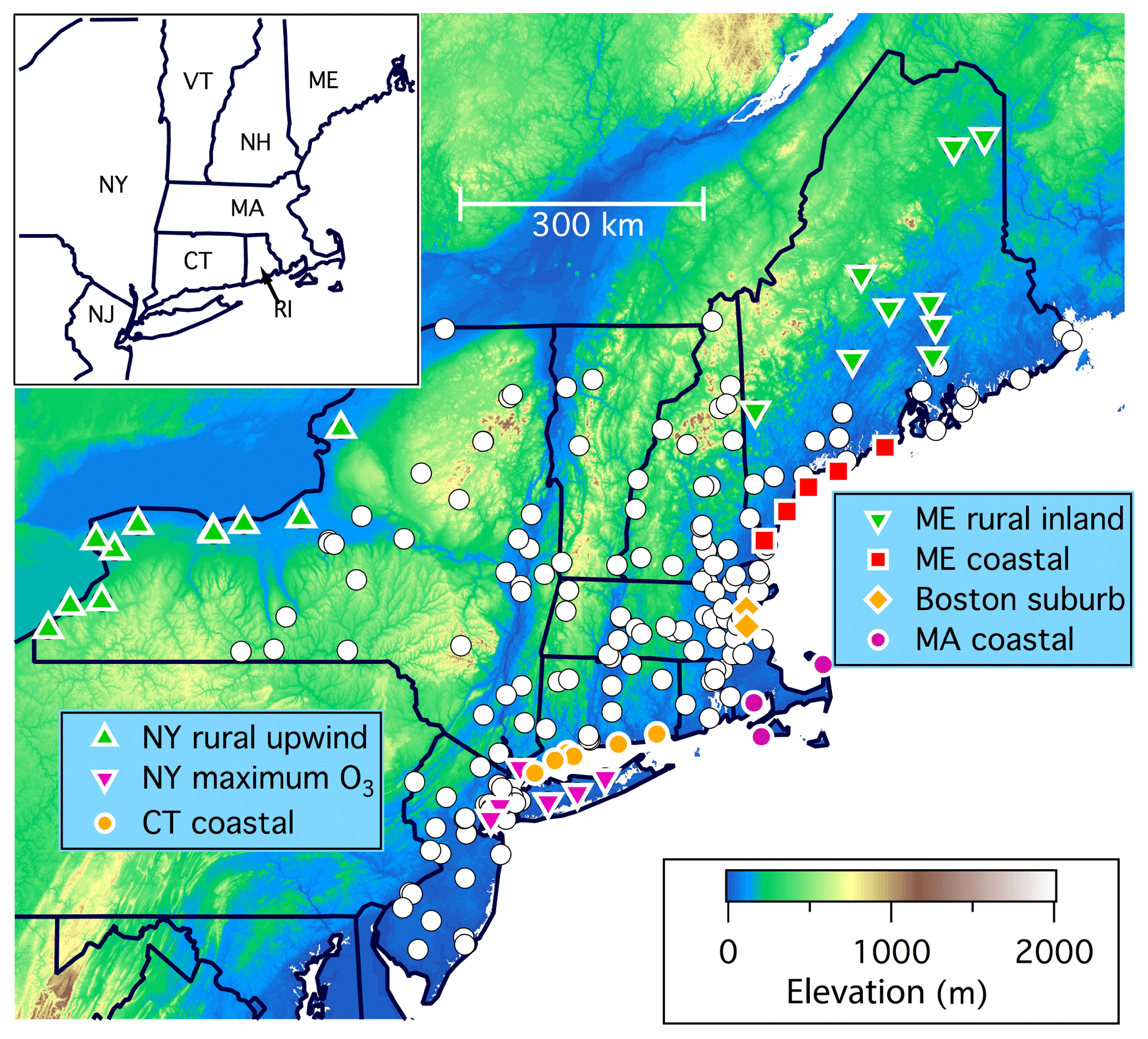
Figure 2Topographical map of the eight northeastern states, with symbols indicating the locations of the ozone monitoring sites. Seven groups of colored symbols indicate groups of sites that are discussed in detail. The inset gives the abbreviations for each of the eight states.
Two northern US regions (maps in Figs. 1, 2, and S1 in the Supplement) are the focus of this work: eight northeastern states, which include the most populated US urban area (New York City metropolitan area), and three sparsely populated rural western states (Montana, North Dakota, and South Dakota), containing no cities with > 260 000 population. The temporal histories of ODVs measured in these two regions (Fig. 3) correlate with the degree of urbanization – in the rural western states they remained approximately constant at relatively small values over the 39 years of measurements, while the largest ODVs with temporally decreasing values have been in the northeastern states. The northern tier of US states also includes three Pacific Northwest states and three midwestern states (map in Fig. S1) with intermediate ODV behavior (Fig. S2); these regions are not examined in detail but are included here for comparison. Notably, none of the ODVs in these regions have approached the maximum ODVs recorded in the SoCAB (indicated by blue lines in Figs. 3 and S2). There are three designated ozone nonattainment areas in the northern US states (based on the 2015 ozone NAAQS – US Environmental Protection Agency (EPA) Green Book: https://www.epa.gov/green-book, last access: 8 July 2019), which include 38 counties in three of the northeastern states – Connecticut, New Jersey, and New York.
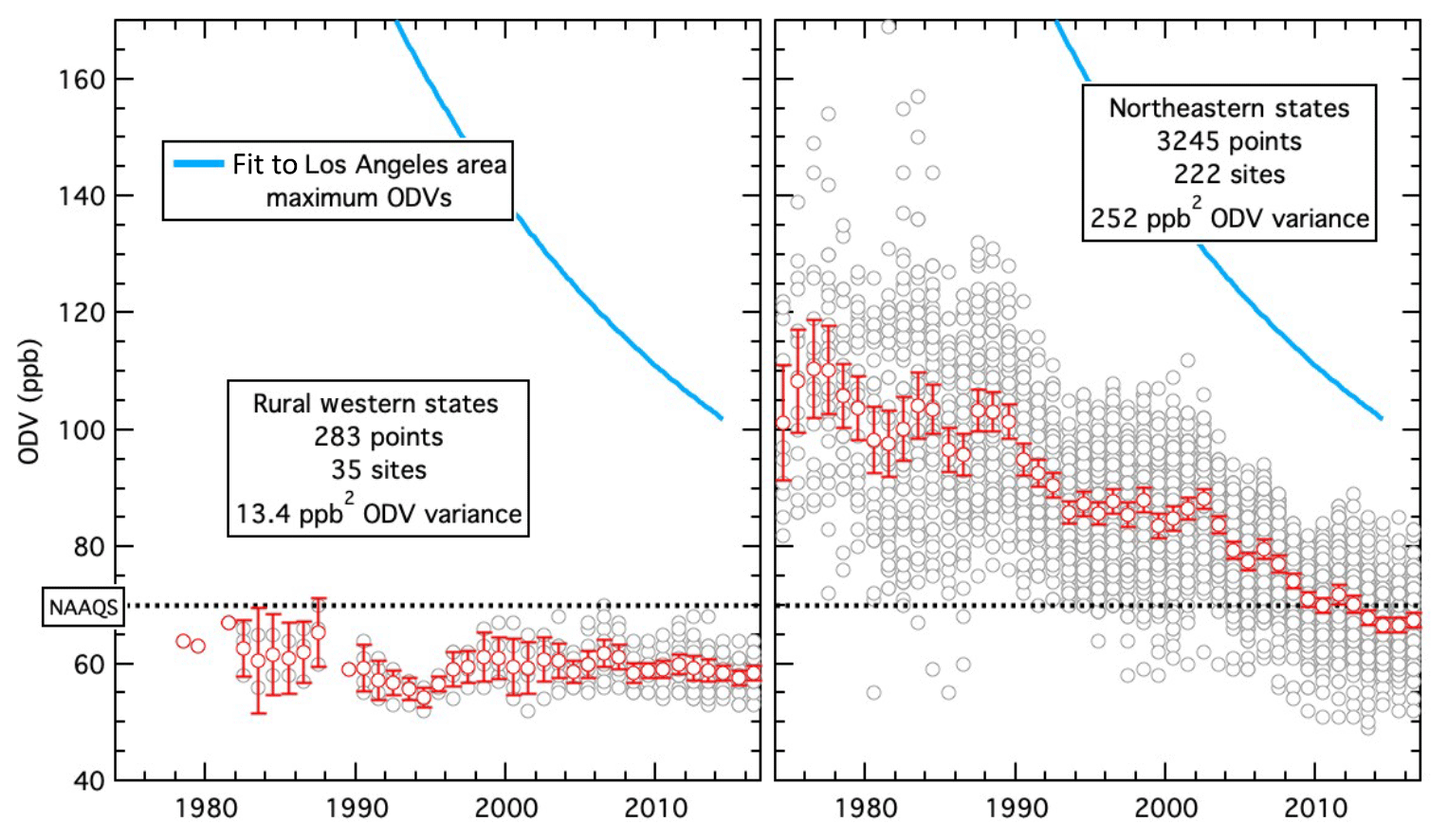
Figure 3Time series of all ODVs (grey symbols) reported from all monitoring sites in the two northern US regions shown in Figs. 1 and 2. The numbers of monitoring sites and reported ODVs and the ODV variance are annotated for each region. The red symbols give the averages and 2σ confidence limits for all ODVs reported in each year. For comparison, the blue curve in each panel indicates a fit to the maximum ODVs recorded in the Los Angeles urban area (Parrish et al., 2017a). The dotted line indicates the 2015 NAAQS of 70 ppb.
In this paper we apply the approach of Parrish et al. (2017a) to examine the temporal and spatial variability in the highest ozone concentrations (i.e., the ODVs) observed over the past 3 to 4 decades in the two contrasting regions of the northern US representing extremes in anthropogenic influence. We separately estimate the US background ODVs and the enhancements of the ODVs above that background contribution due to photochemical production from US anthropogenic precursor emissions. The US background ODV estimates quantify the maximum ozone concentrations that would exist in these regions in the absence of US anthropogenic precursor emissions. We also aim to quantify the temporal evolution and spatial variability in the US anthropogenic ODV enhancements and, based on past trends, project the expected time required for the maximum ozone concentrations to decrease to the 70 ppb NAAQS in the northeastern US.
Photochemical modeling systems are generally utilized for quantifications and projections of ODVs (e.g., Dolwick et al., 2015; Emery et al., 2012; Fiore et al., 2014). However, present model quantifications of US ozone concentrations have large uncertainties (Jaffe et al., 2018; Guo et al., 2018). An observationally based approach such as that presented here provides useful comparisons for the results of modeling efforts, and differences between the two approaches identify needs for further research.
The analysis approach in this paper relies on differences in the temporal behavior of the US background ODV (demonstrated in this work to be approximately constant) and ODV enhancements resulting from US anthropogenic precursor emissions; these enhancements have greatly decreased over recent decades in response to US emission controls. Previously published studies have identified a multitude of additional processes that can potentially make systematic contributions on a variety of timescales to the variability in ozone concentrations at US surface sites; however there has been little in the way of systematic, quantitative analysis of their effects on ozone concentrations across the US. In this work, we first quantify the US background ODVs and the temporal decrease in US anthropogenic ODV enhancements and then discuss the influence of other processes through examination of the fraction of the ODV variance not accounted for by decreasing US anthropogenic ODV enhancements.
Papers investigating US surface ozone trends (see Lin et al., 2017, and references therein) have treated a variety of statistics (medians, means, and various percentiles) to characterize ozone concentrations. In this work all trends are based on ODVs. The reason for this choice is that the NAAQS is based on this statistic, and thus it is most relevant for policy considerations. The ODV corresponds to approximately the 98th percentile of the MDA8 concentrations during the ozone season. As a consequence, the US background ODVs that we discuss are significantly larger than average or median background ozone concentrations examined in other studies. Given these different choices, care must be taken in comparing trends derived in this work with those from other analyses.
The sources of data and the analysis methods are discussed in the next section, followed by the applications of those methods to quantify the US background ODVs and the US anthropogenic enhancements in the rural western region (Sect. 3.1) and the northeastern US (Sect. 3.2). The larger temporal ODV trends and the greater spatial variation in those trends in the northeastern US provide the basis for the elucidation of several features of regional ozone concentrations. Section 3.3 examines the uncertainty of the analysis approach used in Sect. 3.2. Section 4 gives a summary of the approach and the results, discusses implications of those results, and identifies needs for further research.
2.1 Ozone design values analyzed
This work considers ODVs reported from the beginning of US ozone monitoring in the mid-1970s through 2017 in 17 northern US states. An ODV, the statistic upon which the US NAAQS is based, is calculated every year for each ozone monitoring station in the US if the measurements achieve the specified completeness criteria. Each year all recorded ODVs are added to EPA's Air Quality System data archive (https://www.epa.gov/aqs, last access: 23 June 2019). All ODVs reported for the northern states were downloaded from this archive; only the ODVs marked as valid were retained for analysis. Exceptional events that have concurrence from the US EPA were excluded. Table S1 summarizes these archived ODVs for each state, including the number of monitoring sites, the years spanned by the reported ODVs, and their maximum and minimum values. The reported ODVs span the range from 169 to 41 ppb. Yellowstone National Park (NP) in another state (Wyoming) is also included because its measurement record has been examined in previous analyses of long-term trends of US background ozone concentrations (e.g., Lin et al., 2017). It should be noted that very few sites have continuous measurements over the indicated time spans and that many sites operated for only short periods. All reported ODVs are included in this analysis even if only a single ODV was reported for a particular site. It is implicitly assumed that the temporal discontinuities associated with initiation or termination of individual sites do not prevent an accurate quantification of temporal trends of ODVs within the regions selected for analysis.
2.2 Exponential ODV trend analysis
A well-established conceptual model (e.g., Parrish et al., 1986) guides our analysis. Ambient ozone concentrations at US surface sites are composed of two contributions: (1) background ozone and (2) enhancements resulting from ozone produced from photochemical processing of US anthropogenic emissions of ozone precursors. The first contribution is the ozone that would be present in the absence of US emissions of ozone precursors from anthropogenic sources; this ozone is transported into the US or produced over the US from naturally emitted precursors. The US EPA has defined this contribution as US background ozone (e.g., Dolwick et al., 2015). The first contribution has remained relatively constant, while the second contribution has greatly decreased over the past 2 to 4 decades in response to reductions in anthropogenic emissions of ozone precursors.
In this work we focus on the time period of decreasing ODVs. Fitting observational data to a simple functional form is a common tool utilized for quantitative observational analysis; linear trend analysis (i.e., fitting observational data to a linear function) is one example. Here we choose to fit observed ODVs to Eq. (1),
with three undetermined parameters. This equation is the simplest possible functional form consistent with the guiding conceptual model of a background contribution and a consistently decreasing anthropogenic contribution. (A linear fit with only two undetermined parameters – slope and intercept – is simpler but cannot fit a positive background contribution, as a decreasing linear fit will eventually go negative.) We identify the first term of Eq. (1), y0, as an estimate of the ODV that would result from US background ozone alone (i.e., consistently called US background ODV) and the second term as an estimate of the enhancement of observed ODVs above y0 (i.e., consistently called US anthropogenic ODV enhancement) due to contributions from photochemical processing of US anthropogenic precursor emissions. This second term decreases exponentially with a time constant of τ and equals A in the reference year, which we choose as 2000.
A simple intuitive argument suggests that an exponential decrease in the anthropogenic ozone contribution is expected to be a reasonable approximation for the response of maximum ozone concentrations to implementation of emission controls. When controls are initiated, early progress can be rapid, since large existing emission sources evolved without planning for their control. With time, reducing emissions will become progressively more difficult, since the most easily controlled emissions will likely be addressed first, and the smaller, remaining emissions will be more difficult and/or expensive to control. This expected increasing difficulty in reducing emissions may well lead to an approximately constant fractional decrease in anthropogenic ozone enhancements, which corresponds to an approximately exponential decrease in these enhancements.
A previous analysis (Parrish et al., 2017a) quantified the temporal evolution of the maximum ODVs in seven southern-California air basins over the 1980–2015 period (shorter periods beginning later and ending in 2015 in two basins). That work utilized fits to Eq. (1) (with the reference year 1980 instead of 2000) and showed that a single value of years, a single value of ppb, and a different value of A in each air basin provided an excellent fit (r2=0.984) to the ODVs in all of those air basins.
As we will see in the following analysis, in the northeastern states the period of consistently decreasing ODVs (generally 2000 and later, hence the choice of 2000 as the reference year in Eq. 1) is too short to allow precise determinations of all three parameters of Eq. (1) from fits to individual ODV time series. In the face of this difficulty, our primary analysis approach is to assume that the τ value (21.9 years) derived for southern California is also appropriate for the northeastern states. Uncertainty in the value of τ is then the greatest source of uncertainty in the analysis results; the impact of this uncertainty will be addressed in Sect. 3.3.2.
Equation (1) assumes that decreasing US anthropogenic ODV enhancements is the only cause of ODV variability at a particular location. Other factors (e.g., rising anthropogenic emissions in Asia, variable occurrences of wild fires, interannual meteorological and climate variability, etc.) can also potentially affect observed ODVs. The approach taken here is to interpret the observed ODVs initially on the basis of Eq. (1) and to examine the fraction of the ODV variance captured by that interpretation. The remaining fraction of the variance is then attributed to other factors, including those listed above. We use three statistics to quantify the variance in the total data set and the fraction not captured by Eq. (1). The total variance in a data set is the square of the standard deviation of those data (in units of ppb2). The root-mean-square deviation (RMSD) between the derived fit and the observed ODVs gives an absolute measure (in ppb) of the ODV variability about the fit; the square of the RMSD (in units of ppb2) gives an estimate of the variance not captured by the fit. The square of the correlation coefficient (r2) between the observed ODVs and the values derived from the fit to Eq. (1) gives a measure of the fraction of the total variance that is captured by that fit; the difference between unity and the r2 value is then a relative measure (as a fraction) of the ODV variance not captured by Eq. (1). In the southern-California air basins (Parrish et al., 2017a), the derived r2=0.984 and RMSD ≈4 ppb indicate that all factors not included in Eq. (1) account for no more than 1.6 % of the total variance in the basin maximum ODVs analyzed in that work and contribute a RMSD to those ODVs of no more than ∼4 ppb.
A potential complication in the interpretation of the two terms of Eq. (1) arises if there is a significant fraction of US anthropogenic ozone precursor emissions that have not been reduced by emission controls. Ozone produced from such emissions will not have decreased in the same manner as that produced from most US anthropogenic emissions, which could raise the derived value of y0 above the actual US background ODV. Parrish et al. (2017a) have discussed this issue with regard to the emissions associated with the intense agricultural activity in the Imperial Valley of the Salton Sea air basin, where the derived y0 is higher than in other southern-California air basins. The final section of this paper briefly considers the possible impact of this complication in the northeastern US states. One difference between the application here and that of Parrish et al. (2017a) should be noted. The former work chose 1980 as the reference year, while here we choose the year 2000. The curves derived from the fits to Eq. (1) and the values derived for the y0 parameter do not depend on the choice of reference year, while the values derived for the A parameter do. Consequently, comparing the A parameters derived here with those given for California by Parrish et al. (2017a) requires adjustments for this difference, which can be provided through the second term of Eq. (1).
2.3 Additional observation-based analyses of ODV time series
Acknowledging the uncertainty introduced by the assumptions required to implement the exponential analysis described in Sect. 2.2, we derive y0 through three additional, somewhat different approaches that also provide two estimates of τ appropriate for the northeastern states.
An independent analysis approach discussed in Sect. 2.3 of Parrish et al. (2017a) can estimate US background ODVs without assuming any specific functional form for the time dependence of the ODV enhancements. Different assumptions underlie this analysis – namely that all of the ODV time series under consideration follow the same functional form, but not necessarily an exponential decrease, and that all time series are approaching a common US background ODV (i.e., y0 value). These assumptions imply that all of the time series will converge to a common ODV as anthropogenic precursor emissions are reduced to zero; this common ODV is necessarily the regional US background ODV. In practice this analysis uses correlations between time series of ODVs with US anthropogenic ODV enhancements that differ as much as possible. One time series is selected as a reference; in the examples discussed here the time series with the largest US anthropogenic ODV enhancements is selected. Other time series are then linearly correlated with this reference. The intercept of each linear correlation with the 1:1 line then provides an estimate of the US background ODV; at that point the ODVs from the two time series are equal. Parrish et al. (2017a) show that the results of this approach for seven southern-California air basins are nearly identical to the results from fits to Eq. (1). We apply this approach to estimate US background ODV in the northeastern US and compare the results to those from the exponential analysis.
Two additional approaches can approximately quantify the value of τ in the northeastern states; both of these approaches assume that constant values of y0 and τ are appropriate for all ODV time series included in each analysis. First, a linear fit to the initial period of decreasing ODVs provides direct information regarding the magnitude of τ and y0. The absolute value and the time derivative of Eq. (1) when evaluated at year 2000 are y0+A and , respectively. Fits to two ODV time series provide four parameters (, and A2) if the τ and y0 values are the same for the two time series. Algebraic manipulation gives , where Δ indicates the difference in the subscripted parameter between the two linear fits, and y0= (, where Σ indicates the sum of the subscripted parameter from the two fits. A complication with this approach is that the linear fits to time periods of significant length give biased measures of the derivative and year-2000 value of Eq. (1); however, this bias can be corrected to first order through numerical comparison of a linear fit to the selected period of the exponential fit. The second approach is described in Sect. 2.4 of Parrish et al. (2017a) and is adapted here to the northeastern-US ODV time series. It uses an iterative, nonlinear regression analysis that simultaneously derives values for τ and y0, plus the A parameter for each ODV time series included in the analysis. This analysis will be adapted to the northeastern-US ODV time series. These two additional approaches help to constrain the uncertainty of the assumed value of τ (21.9 years).
2.4 Confidence limits and uncertainties
In this work we consistently give 95 % confidence limits for derived parameters, unless indicated otherwise. Most of the analysis in this work is based on nonlinear, least-squares regression fits of the archived ODVs to Eq. (1), and interpretation of the derived values for y0 and A. In this interpretation it is important to properly consider the uncertainty of these values. We begin with the 95 % confidence limits given by the least-squares fitting routines, which are then adjusted to account for the known covariance between the recorded ODVs. Each ODV is a 3-year running mean; therefore only every third ODV is independent of the others determined at a given site. Consequently, the number of independent ODVs in each fit is smaller than the number of reported ODVs by approximately a factor of 3. Thus, all confidence limits derived from the fitting routines have been increased by a factor of 31∕2 to account for this covariance. Note that the confidence limits are typically one to a few parts per billion; thus results and their confidence limits are often given to 0.1 ppb precision even though the last significant figure is likely not justified.
There are additional sources of covariance between the ODVs included in any particular fit. The ODVs from different sites within a region can covary due to regionally coherent interannual variability, and interannual variability may lead to covariance between ozone concentrations measured in successive years. We are not able to account for the effect of this additional covariance; the derived confidence limits are thus lower limits for the true confidence limits of the derived parameters. However, as discussed in the next section, we can find no indication that additional regional or temporal covariance of the ODVs makes significant contributions to the uncertainties of the results. The influence of often-cited major drivers of temporal variation in ozone, which could possibly cause such covariance, is discussed in Sect. 4 and found to be small.
Here we examine the time series of ODVs from the western rural states (Sect. 3.1), fit the time series of ODVs from the northeastern states to Eq. (1) (Sect. 3.2), and discuss the results in the context of the conceptual model introduced above. This model considers the recorded ODVs to comprise two contributions: (i) an approximately constant US background ODV identified with y0 in Eq. (1) and (ii) US anthropogenic ODV enhancements, which are approximated by the second term in Eq. (1). Sections 3.2 and S1 of the Supplement discuss further details of the spatial and temporal variability in ODVs in the northeastern states. Section 3.3 uses the alternative approaches described in Sect. 2.3 to examine the uncertainty inherent in the parameter determinations from the exponential analysis using Eq. (1).
3.1 ODVs in rural western states
The sparsely populated, three-state, rural western region generally lies on the northern US Great Plains downwind of more mountainous terrain to the west. Figure 1 shows a topographical map of the region, with the locations of the ozone monitoring sites indicated. This area gradually slopes to the east and north. All of the monitoring sites lie below 1.55 km elevation, with the exception of Yellowstone NP at 2.43 km.
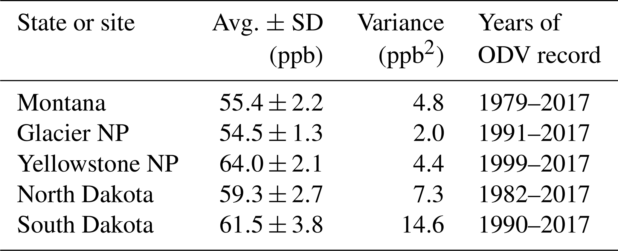
The histories of the ODVs recorded in the region are illustrated in Figs. 3 and 4, and averages with standard deviations and variances are given in Table 1. The gaps in the Montana and South Dakota records were caused by extended periods when no valid ODVs were recorded at any site within the respective states. Throughout the ODV record there is little variability due to any cause. The 283 tabulated ODVs recorded over 39 years at 35 sites in the three states average at 59.3 ppb, with a standard deviation of 3.7 ppb (corresponding to a variance of 13.4 ppb2) – strong evidence that the ODVs correspond to an approximately constant US background ODV within this region with no evidence for significant US anthropogenic ODV enhancements. At the individual sites and within each state the entire measurement records are all well described by averages with small standard deviations (Table 1): < 3 ppb in Montana and North Dakota and < 4 ppb in South Dakota, the state whose sampling sites span the largest elevation range (0.34 to 1.55 km). US background ODVs generally increase with the elevation of the sampling site (e.g., see discussion in Jaffe et al., 2018), so larger variability is expected when the monitoring sites within a state span a larger range of elevations. The state averages in Table 1 lie within a range of ∼6 ppb, but there are some significant differences: a maximum in South Dakota (61.5 ppb) and a minimum in Montana (55.4 ppb), with North Dakota being intermediate (59.3 ppb). Consistent with the site elevation differences, the average ODV at Yellowstone NP is significantly larger than that at Glacier NP: 64.0 ppb at 2.43 km and 54.5 ppb at 0.96 km, respectively. The variances in the data sets vary from 2 to 15 ppb2; these values indicate that only small variance in long-term ODV records can arise from variation in US background ozone alone, at least in this particular region of the country.
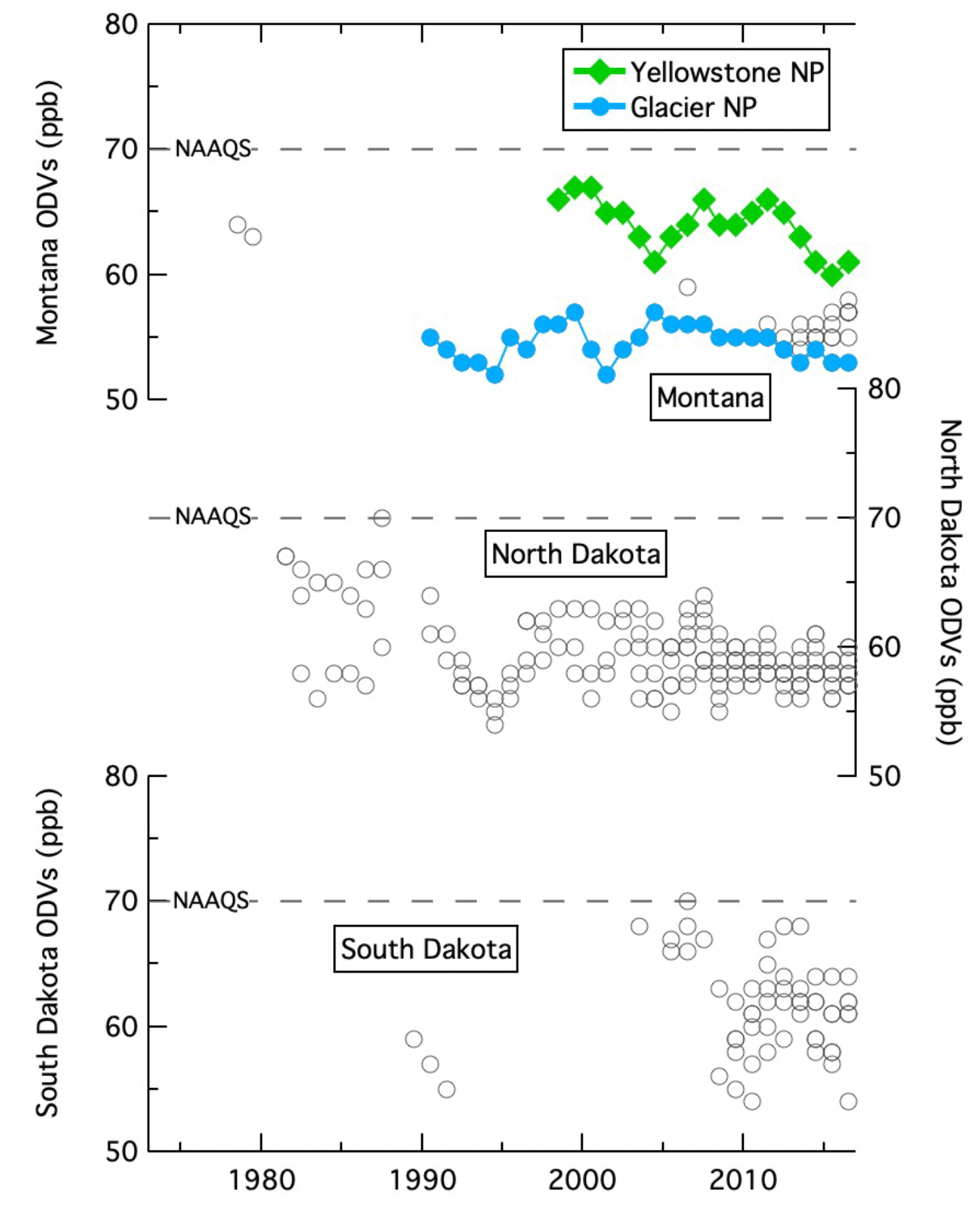
Figure 4Time series of all ODVs (grey symbols) reported from all monitoring sites in three rural western states plus Yellowstone NP, located in Wyoming. The two sets of colored symbols are results from two long-term sites in national parks.
3.2 Exponential fits to ODVs in northeastern states
A topographical map showing the networks of ozone monitoring sites in the eight northeastern US states is given in Fig. 2. All of the ODVs recorded in four of the eight states are plotted in Figs. 5 and 6 along with curves showing fits of Eq. (1) to the ODVs from selected groups of sites over selected time periods. These ODV time series are in striking contrast to those in the rural western states (compare Figs. 5 and 6 with Fig. 4), with much larger concentrations showing strong decreases over the past 2 to 3 decades and much greater variability in ODVs. We attribute this contrast to the much greater influence of US anthropogenic ODV enhancements in the northeastern states. The greater variability is quantitatively reflected in the ODV variance in this region (252 ppb2), which is nearly a factor of 20 larger than that seen in the rural western states; this comparison shows the dominant influence of the US anthropogenic ODV enhancements in the northeastern states.
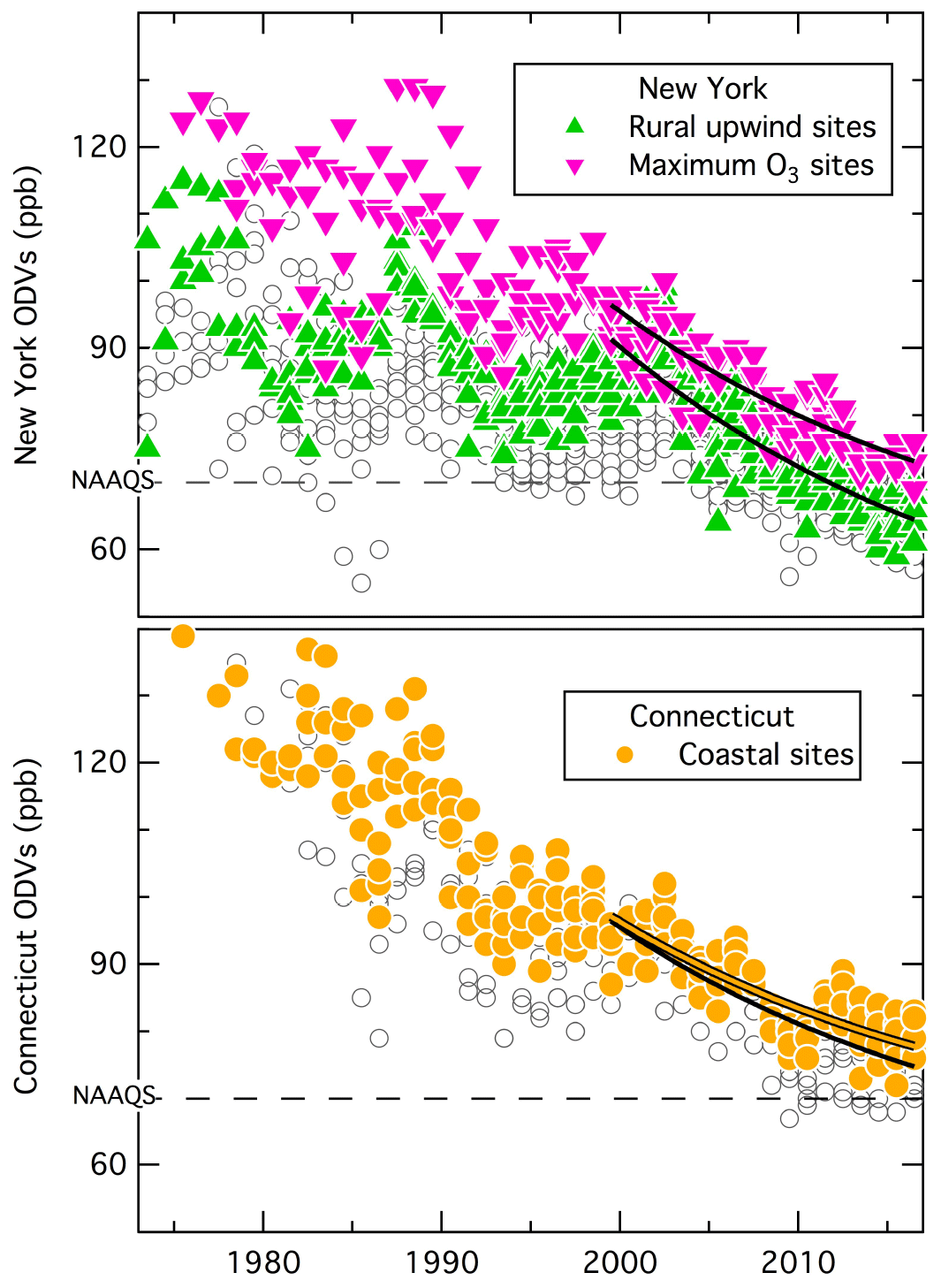
Figure 5Time series of all ODVs (grey symbols) reported from all monitoring sites in New York and Connecticut. The three sets of colored symbols indicate the results from groups of sites that are discussed in detail. The curves are fits of Eq. (1) to respective colored symbols and to all data points for Connecticut.
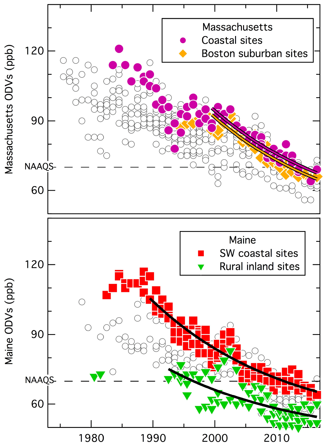
Figure 6Time series of all ODVs (grey symbols) reported from all monitoring sites in Massachusetts and Maine. The four sets of colored symbols indicate the results from groups of sites that are discussed in detail. The curves are fits of Eq. (1) to respective colored symbols.
The four states included in Figs. 5 and 6 are shown for illustrative purposes, with Figs. S3–S10 of the Supplement showing detailed ODV temporal plots and fitted curves to the selected groups of sites in all eight states. These groups of sites were selected to represent different environments within each state, with the expectation that similar temporal ODV trends will be found at all sites within each group. The strategy adopted is to fit the ODVs recorded at all sites within each group over the time period beginning when a clear, consistent decrease in ODVs is first established and continuing through 2017, the most recent year for which ODVs are available. This strategy is required since Eq. (1) is designed to provide fits to ODVs only during such periods of consistent decreases. In all cases these fits begin by 2000, with some beginning earlier – either at the start of measurement record, in 1990, or in 1995, determined by the best, consistent fit to the functional form of Eq. (1). Figures S3–S10 include maps indicating the locations of all selected groups of sites. In all, 17 groups within the eight states were selected; they are listed in Table 2 along with the parameters derived from the fits of Eq. (1).
Table 2Results of least-squares fits to Eq. (1) illustrated in Figs. 5–7 and S3–S10; RMSD indicates the root-mean-square deviation between the observed ODVs and the derived fit.
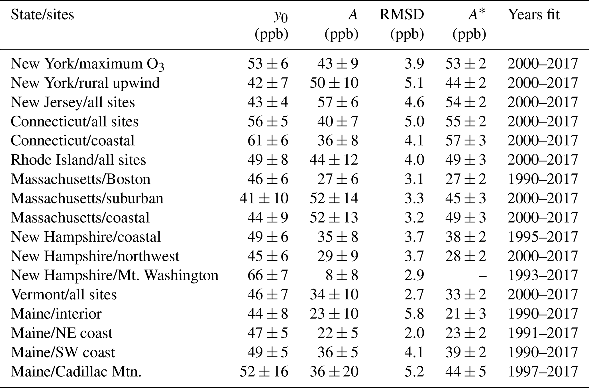
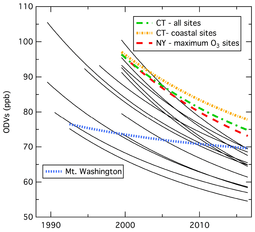
Figure 7Comparison of fits of the ODVs from 17 groups of sites in eight northeastern US states shown in Figs. 5, 6, and S3–S10 to Eq. (1). The parameters of these fits are included in Table 2.
There are some consistent general features of the ODV time series and the corresponding fits that inform the following analysis.
Throughout the measurement record, the largest ODVs are found in the states that contain the New York City metropolitan area (New York, New Jersey, and southwestern Connecticut) or that lie directly downwind (coastal Connecticut and Long Island, New York). Such sites compose two of the selected groups of sites in New York and Connecticut (see highlighted points in that area in the map of Fig. 2), whose ODVs and fits of Eq. (1) are highlighted in Fig. 5.
In several states, the largest ODVs are recorded at coastal sites (i.e., Connecticut, Massachusetts, New Hampshire, and Maine in Figs. 5, 6, S5, S7, S8, and S10). The large ODVs at coastal sites emphasize the important, widely discussed (e.g., Wolff and Lioy, 1980; Wilcox, 1996) role of transport in bringing high ozone concentrations from the major East Coast urban areas far downwind, particularly when that transport occurs over the waters of the Long Island Sound and the coastal Atlantic Ocean. Two relatively isolated Massachusetts coastal sites on the offshore island of Martha's Vineyard and near the tip of Cape Cod record some of the highest ODVs within that state (see Fig. S7). Dukes County, which includes only Martha's Vineyard, with a total population of ∼17 000, was once designated as a marginal non-attainment area for ozone.
In the past, ODVs at rural, generally upwind sites on the western border of New York (green symbols in on the left in Fig. 2) were significantly smaller than in the northeastern US urban areas, although in recent years that difference has diminished (Fig. 5). These upwind rural areas in New York, and similar sites in Vermont (Fig. S9), experienced ozone concentrations exceeding 80 ppb throughout the measurement record until about 2005. These high concentrations caused Chautauqua County, New York, with a population of ∼95 000, to also once be designated as a marginal non-attainment area, again emphasizing the importance of ozone transport in the northeastern US, although in this case the source of the transported ozone is not as clearly established.
Additional systematic features of the ODV time series in the northeastern US are discussed in Sect. S1 of the Supplement.
All of the curves derived from the fits of Eq. (1) to the long-term trends of the ODVs shown in Figs. 5, 6, and S3–S10 are compared in Fig. 7, with the corresponding parameters included in Table 2. Except for the four fits denoted by the colored dotted and dashed curves, all fits are similar in the sense that they exhibit the same relative long-term decrease and are asymptotically approaching approximately the same value of y0. The same relative long-term decrease is necessarily forced by the use of the same value of τ=21.9 years in all fits. However, the derived A and y0 values do provide information regarding the spatial and temporal variation in ODVs over the past 2 to 3 decades. Three of the four curves with noticeably different behavior are from fits to the groups of sites with the highest recently reported ODVs (Connecticut, especially the coastal sites, and the New York sites highlighted in Figs. 2 and 5); these are discussed further in Sect. S1 of the Supplement. The fourth exception is the one high-elevation site (Mt. Washington in New Hampshire at an elevation of 1.9 km), which is also discussed separately in Sect. S1. The parameters in Table 2 provide the basis for quantitatively comparing the fits throughout the northeastern US in the next two sections.
3.2.1 Estimation of US background ODV in northeastern states from exponential fits
All y0 values in Table 2 (excluding the four exceptions indicated in Fig. 7) agree with each other within their indicated confidence limits. The arithmetic mean of these y0 values is 45.9 ppb, with a standard deviation of 3.2 ppb. The average of these y0 values weighted with the inverse square of the respective confidence limits is 45.8±1.7 ppb, where the 95 % confidence limit of this average is indicated. All of the y0 values in Table 2 agree (again excluding the four exceptions noted above) with these average values within their indicated confidence limits. Figure S11 of the Supplement shows the distribution of the y0 determinations; 13 of the 17 derived y0 values approximately define a normal distribution, with a median of 47.7 ppb and a standard deviation of 4.5 ppb. The median is interpreted as representing a common regional y0 value, and the standard deviation is interpreted as reflecting the uncertainty in determining each y0 value. This median is consistent with the above averages. The highest 4 of 17 derived y0 values define a high-value tail; these are the four exceptions indicated in Fig. 7.
Recalling earlier discussion, we identify the average y0=45.8 as the best estimate of the US background ODV throughout the northeastern US; there is no discernable spatial variability within this region. This value is significantly smaller than the value of 62.0±1.9 ppb derived for southern California (Parrish et al., 2017a); however even at this smaller value, the US background ODV in the northeastern US amounts to 65 % of the 70 ppb NAAQS.
3.2.2 Estimation of US anthropogenic ODV enhancements in northeastern states from exponential fits
The fits to Eq. (1) with τ=21.9 years provide estimates of A, the US ODV enhancement in the reference year 2000; Table 2 lists these values for the 17 selected groups of sites from two-parameter fits, i.e., fits with y0 and A as independent parameters determined from the least-squares fits themselves. However, the results above show that a constant value of ppb is characteristic of the entire northeastern US region. Using this result allows fits of Eq. (1) to all groups of sites without the larger uncertainty in the y0 derived from the individual fits. Consequently, results of one-parameter fits of Eq. (1) (i.e., with y0 held constant at the value of 45.8 ppb) are included in Table 1 as the A* values. (Such a fit is not included for the Mt. Washington results, since US background ODV is evidently greater than 45.8 ppb, as discussed in Sect. S1 of the Supplement.) The A* values generally agree with the A values from the two-parameter fits within their confidence limits, which are smaller, since only one parameter needs to be derived. The exceptions to the agreement between A and A* are the fits to the exceptions discussed earlier – the two groups of Connecticut sites and the New York maximum ozone sites, which are the upper three colored curves in Fig. 7. In Table 2 the A values for these three groups of sites are anomalously small compared to the results from neighboring groups of sites (i.e., New Jersey, Rhode Island, and Massachusetts/coastal); the A* values for all of these neighboring groups of sites agree more closely. In the following discussion we take these A* values as the best estimate for the US anthropogenic ODV enhancements in the northeastern states.
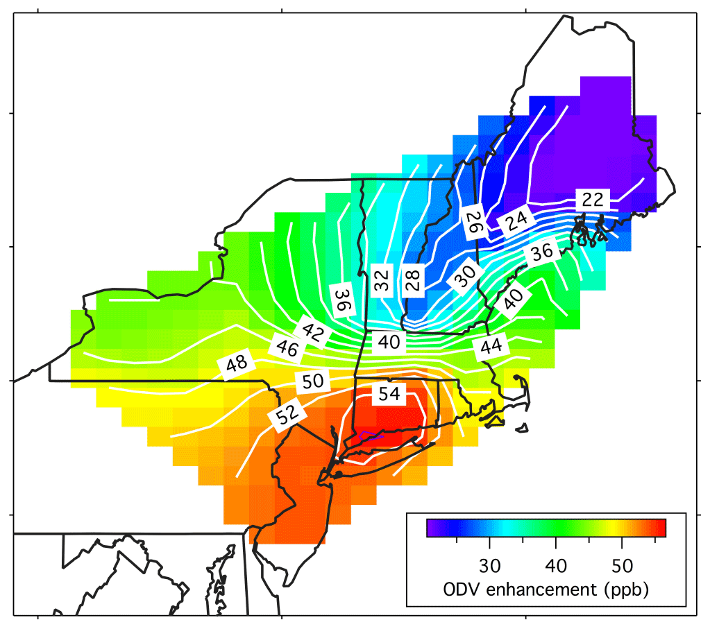
Figure 8Approximate contour plot of the US anthropogenic ODV enhancement due to photochemical production from precursor emissions in the year 2000, estimated from the A* values given in Table 2.
A contour plot (Fig. 8) derived from the A* values in Table 2 provides an overview of the spatial variation in the US anthropogenic ODV enhancements across the northeastern US. The groups of selected sites fit to Eq. (1) give only coarse spatial resolution across the region, so the contour plot has uncertainties not apparent from the smooth spatial variability in this figure. This uncertainty has been mitigated in deriving the contour plot by including duplicate A* values at the site locations in each selected group of sites; these additions ensure that the contouring program reproduces a more nearly constant value over the sometimes-large regions covered by the selected groups of sites. Despite the uncertainties, the contour plot does give a useful, semi-quantitative representation of the magnitude and regional variation in the US anthropogenic ODV enhancements in the region. Note that the contour plot and the A and A* values of Table 2 describe the ODV enhancements in the year 2000. As is apparent from Eq. (1) and the illustrated temporal trends in the figures, the ODVs have decreased throughout the last 2 to 3 decades. The e-folding time of τ=21.9 years implies that between the reference year of 2000 and 2017, the ODV enhancements decreased by a factor of 2.2. Hence, dividing the year-2000 ODVs in the contour plot by that factor gives an approximation of the 2017 US anthropogenic ODV enhancements.
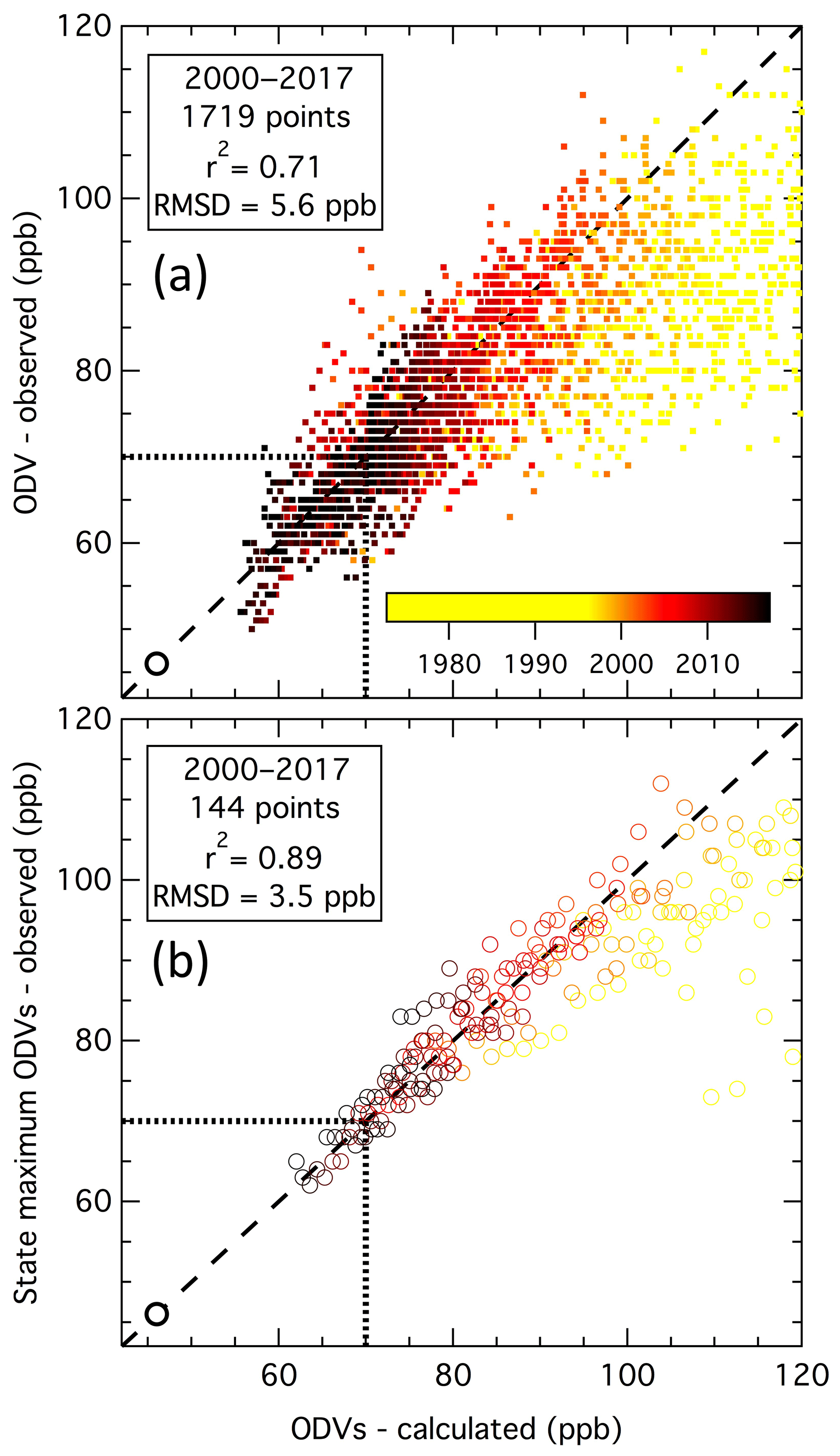
Figure 9Comparison of observed ODVs color-coded by year with those calculated from Eq. (1) for (a) all monitoring sites and (b) for the maximum observed in each state. The dashed lines indicate the 1:1 relationships, with y0 near the origin indicated by the larger circle. The dotted lines indicate the NAAQS. The number of data points, square of the correlation coefficient, and the root-mean-square difference between the observed and calculated ODVs for 2000–2017 are annotated.
The ability of Eq. (1) to accurately reproduce observed ODVs can be judged by comparing the observed ODVs with the values predicted from the fits derived with y0=45.8 ppb and τ=21.9 years. Figure 9a shows this comparison as a correlation plot. The fits for ODVs recorded at all sites in the eight northeastern states over the entire measurement period are calculated from the A* values at each site interpolated from the contour plot of Fig. 8. The correlation is high (r2=0.71) for the 1719 separate ODVs recorded at the 148 sites over the 2000–2017 period but significantly lower for earlier years as expected from the figures, illustrating the derived fits. A general decrease in ODVs throughout the region did not begin until 2000, which is about the time that the US EPA “NOx SIP Call” began reducing power-plant NOx emissions across much of the eastern US (Aleksic et al., 2013). There is significant scatter about the 1:1 line in the comparison in Fig. 9a; the RMSD between observed and calculated ODVs is 5.6 ppb for the 2000–2017 period. Much of this scatter is due to variability in ODVs recorded at different sites within a given region, which arises from differences in local photochemical ozone production and transport patterns. This variability can be reduced by comparing state maximum ODVs (Fig. 9b) rather than individual site ODVs. Figure 10 plots the time series of these state maximum ODVs recorded in each year with respective fits over the 2000–2017 period. The derived A* values (given in Table 3) are somewhat larger than would be expected from the contour plot in Fig. 8, consistent with consideration of only the maximum ODVs recorded in each state. Stronger correlation (r2=0.89) is found for the fits to the state maximum ODVs as expected, since considering only the largest of the state's ODVs in a given year removes much of the regional variability across the state.
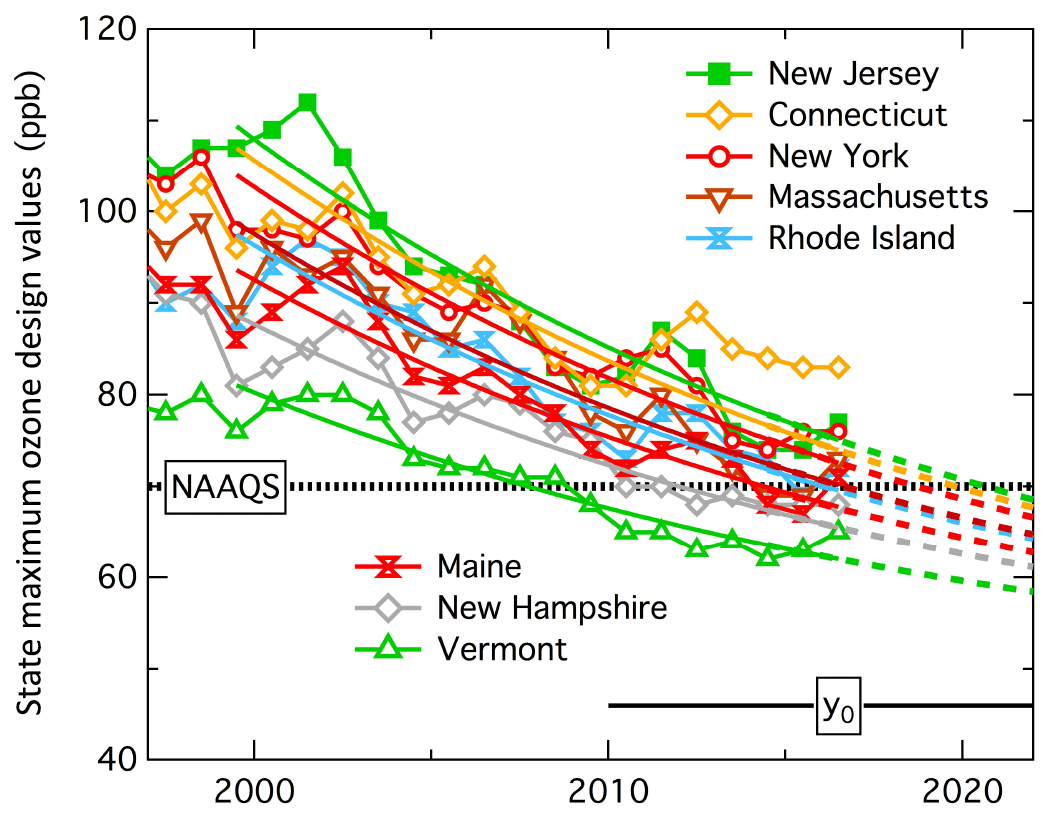
Figure 10Time series of maximum ODVs reported from any site within each of the eight northeastern states. The solid curves are fits of Eq. (1) to the respective colored symbols for the 2000–2017 period. The derived A* values from these fits are given in Table 3. The dashed lines are projections of the solid curves.
Table 3Results of least-squares fits of Eq. (1) to the state maximum ODVs illustrated Fig. 10; y0 and τ were held constant at 45.8 ppb and 21.9 years, respectively. The absolute root-mean-square deviations between the observed ODVs and the derived fits are indicated. YearNAAQS indicates the projected year that the fit to the state maximum ODV drops to the NAAQS of 70 ppb.

3.3 Evaluation of uncertainty of the exponential fits to ODVs in northeastern states
Here the methods described in Sect. 2.3 are applied to investigate the uncertainty of the results from the exponential fits presented in Sect. 3.2. Section 3.3.4 provides an overall assessment of this uncertainty.
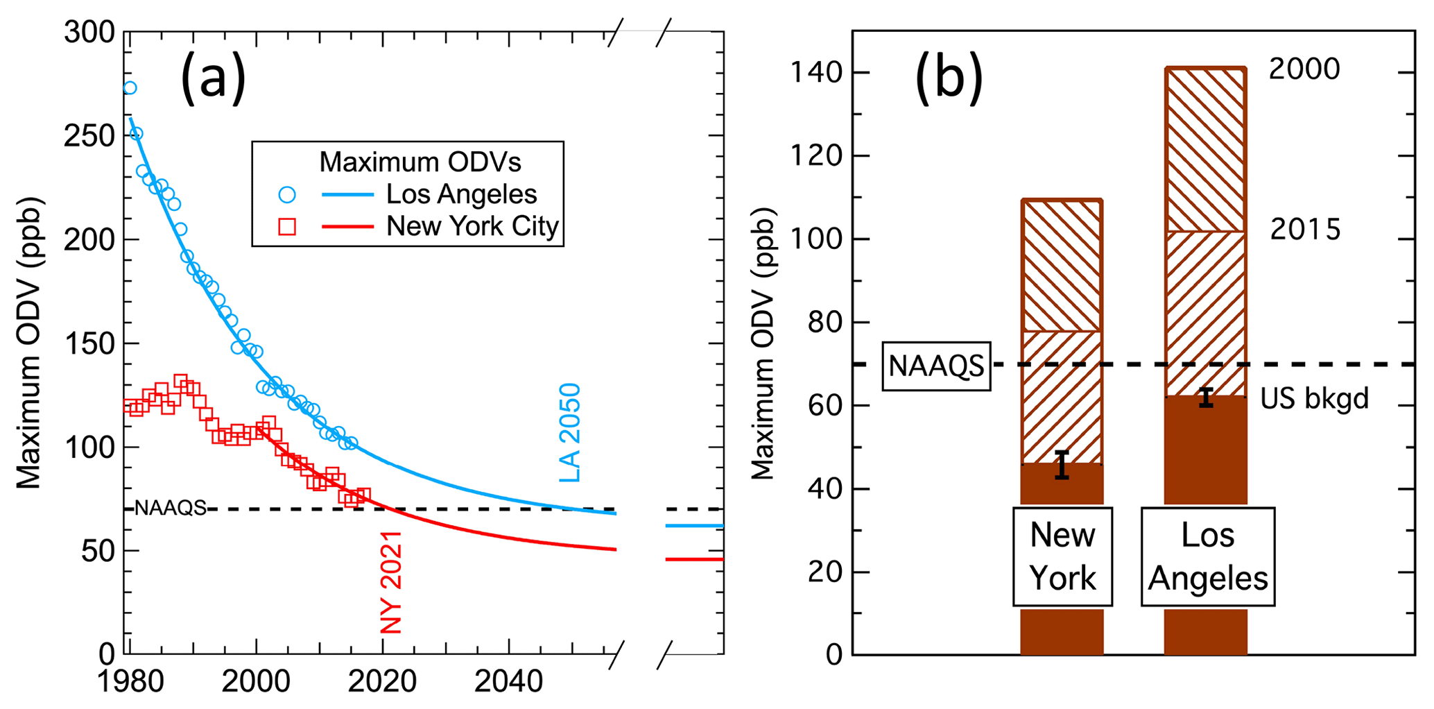
Figure 11Comparison of maximum observed ODVs in the New York City and Los Angeles urban areas. (a) Temporal trend of observations (symbols) and fit to Eq. (1), including extrapolation to infinite time; annotations indicate year that extrapolations decrease to 70 ppb. The New York City results are the maxima from either the states of New York or New Jersey, and the Los Angeles results are those for the South Coast Air Basin (Fig. 8 of Parrish et al., 2017a). (b) Bar graph indicating maximum ODVs in 2000 and 2015 (hatched bars) and the estimated US background (bkgd) ODV (solid bars); the maximum ODVs are derived from the fits to Eq. (1) included in (a).
3.3.1 Alternative approach for estimating US background ODVs in the northeastern US states
The independent analysis approach introduced in Sect. 2.3 can estimate US background ODVs through correlations between separate ODV time series. The ODVs from each of the 13 groups of sites that give the black lines in Fig. 7 are included in this analysis. The reference ODV time series chosen is the maximum observed ODVs in the New York City urban area (NYC urban maximum), which is equated to the maximum ODV observed each year in either New York or New Jersey. These maxima (plotted in Fig. 11a) are all recorded near the New York urban area. This reference is selected because these are among the largest ODVs recorded in the northeastern US, and after 2000 this time series closely follows an exponential decrease with little interannual variability. Figure 12 shows three example linear correlations (the ODVs recorded at the three sets of Massachusetts sites) with that reference. Figs. S12–S18 of the Supplement show all of the linear regressions for the 13 regional data sets, Fig. S19 compares all of the fits, and Table S2 collects the results. These results are quite variable (25 to 62 ppb) due to the relatively short 2000–2017 data records and because the slopes are not widely different from unity, preventing a precise determination of the intercepts of the correlations with the 1:1 line. However, the average of the derived background ODVs (49.2±3.9 ppb for ordinary linear regressions and 42.5±5.7 ppb for reduced major axis regressions, where 95 % confidence limits of the averages are indicated) bracket the result derived from the exponential fits, and neither average is statistically significantly different from that earlier result. The agreement between these two approaches for estimating US background ODVs shows that the assumption of an exponential decrease in the ODV enhancements is not essential for estimating the background ODV (although that approach does give more precise results) and increases our confidence in the results of each approach.
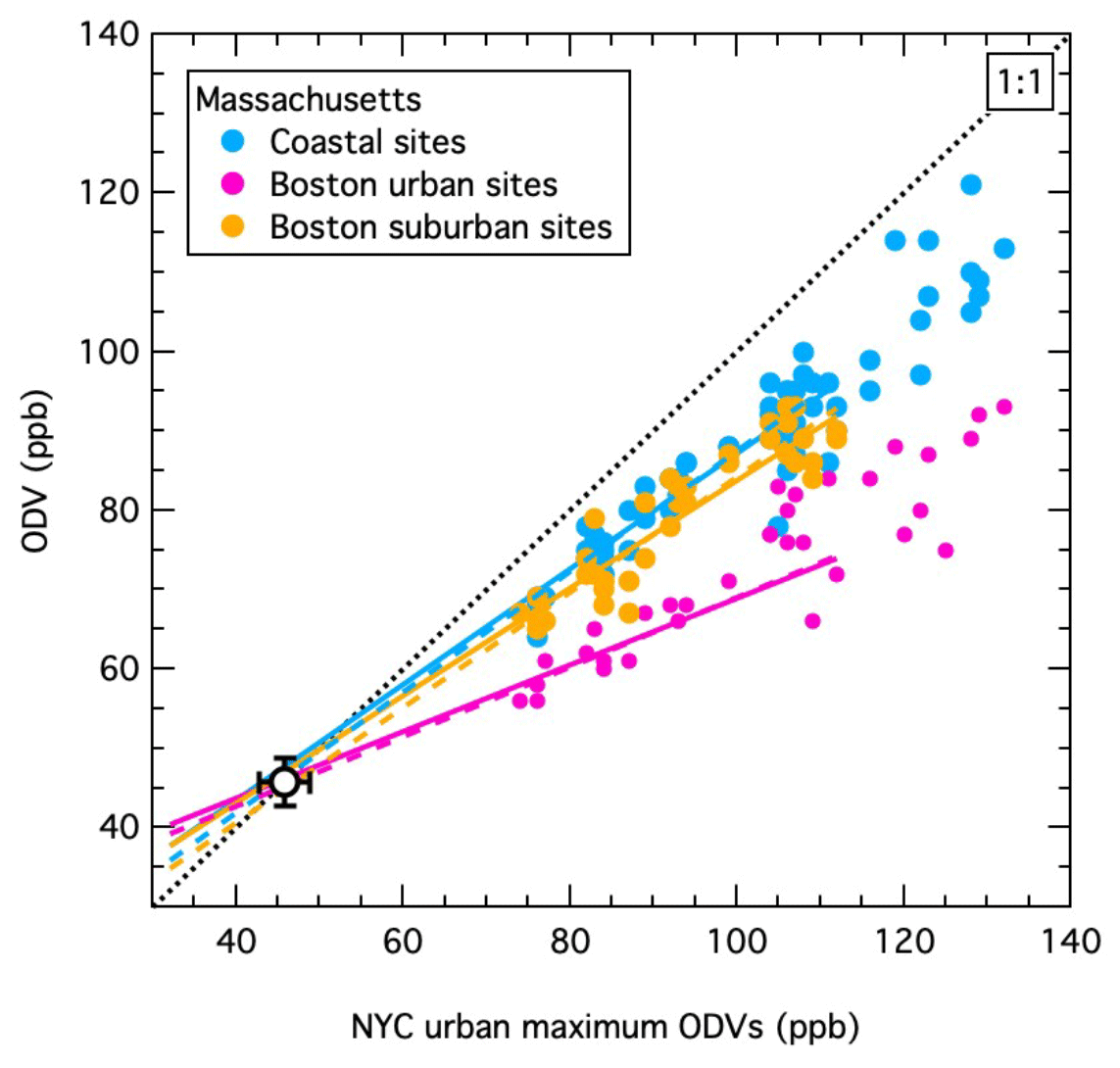
Figure 12Correlation between the ODVs from three sets of Massachusetts sites and the maximum ODVs recorded in the New York city urban area. Lines of corresponding color show ordinary linear regression (solid) and reduced major axis regression with equal weighting (dashed) fits of the correlated data sets for the ODVs recorded in 2000–2017. The black symbol shows the mean US background ODV derived from the exponential fits to the ODV time series, and the dotted line indicates the 1:1 relationship.
3.3.2 Estimate of τ and y0 from linear fits to ODV trends in the northeastern US states
Linear fits to the period of decreasing ODVs for three ODV time series are shown in Fig. 13. These three series were chosen so that one (NYC urban maximum introduced in the previous section) includes the largest ODVs, and two have some of the smaller ODVs in the northeastern US; this choice gives the largest contrast in the absolute year-2000 values and fitted slopes in order to provide the most precise τ and y0 determinations. Table S3 gives the year-2000 values and slopes of those fits, which give zero-order estimates of and y0= (. However, as is apparent in Fig. 13, the year-2000 value and slope derived from each linear fit over the 18-year or 26-year period are biased with respect to the instantaneous value and slope of Eq. (1) in year 2000. This bias can be estimated from linear fits over those same time periods to the exponential curves defined by the zero-order estimates of τ and y0. Table S3 gives year-2000 values and slopes corrected to first order for this bias. These corrected values give and 21.7±5.0 years and y0=48.7 and 47.0 ppb for the fit parameters from the upper and lower Fig. 13 panels, respectively. These τ values compare favorably with the assumed California value (21.9 years), while the y0 values are larger than derived in the analysis using exponential fits to Eq. (1) (45.8±1.7 ppb).
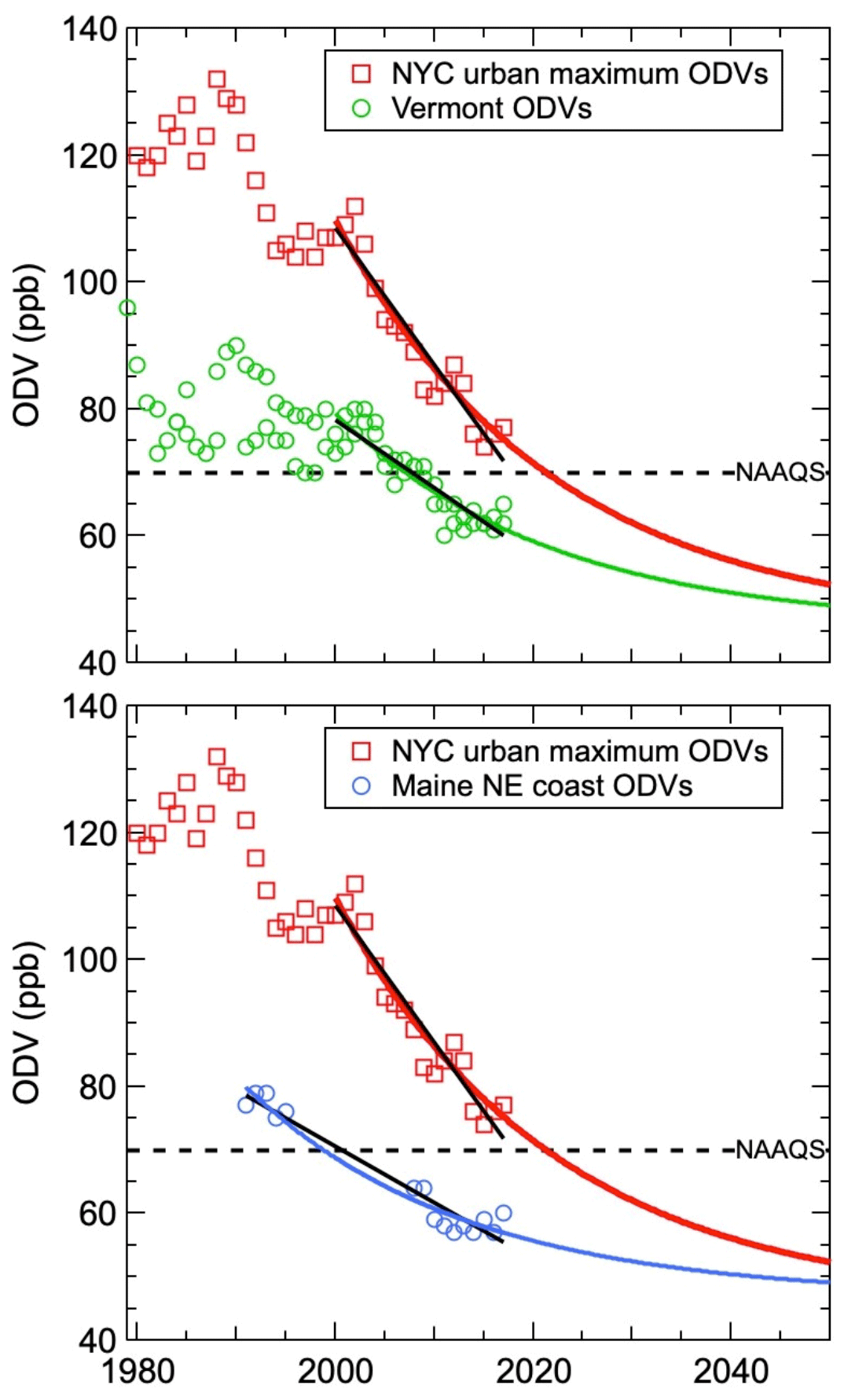
Figure 13Comparison of linear and exponential fits to three ODV data sets. The black line segments are linear fits to 2000–2017 for two data sets and 1991–2017 for one data set. The colored curves are the exponential fits to these time series, also shown in Figs. 11, S9, and S10.
3.3.3 Simultaneous least-squares regression fit to northeastern US state ODV maxima
An iterative, nonlinear regression analysis similar to that described in Sect. 2.4 of Parrish et al. (2017a) and introduced in Sect. 2.3 is applied here to simultaneously fit seven ODV time series to Eq. (1) to determine nine parameter values. The data sets are the 2000–2017 maximum ODVs recorded in seven states plotted in Fig. 10. A simultaneous fit to multiple ODV time series improves the precision of the parameter determinations. Values of τ and y0 (assumed to be the same for all seven states) and values of A for each of seven states are optimized in an iterative process that minimizes the sum of the squares of the deviations between the fit and the original time series. The resulting parameter values are given in Table S4, and Fig. S20 compares the fit results with the original ODVs. The derived τ value (26.0±6.0 years) is larger than the southern-California value of (21.9±1.2 years), although it agrees within the derived 95 % confidence limit. Correspondingly, the derived y0 value (41.8±3.0 ppb) is smaller than that derived earlier (45.8±1.7 ppb), and the A values are larger (compare to Table 3), but again all agree within the derived confidence limits. This fit captures 89.6 % of the variance in the seven ODV time series, comparable to the result shown in Fig. 9b. (Note that since its recent ODV behavior is different from the other states, as discussed in Sect. 3.2, Connecticut is not included in this analysis.)
3.3.4 Assessment of uncertainty of the results
Section 3.2 presents fits of Eq. (1) to ODV time series in the northeastern US derived with an assumed value for τ; all confidence limits given for the derived parameters are lower limits due to this assumption. The above analyses in this Sect. 3.3 investigate alternative approaches to better constrain the overall uncertainty of the results. With regard to the value of τ, the analysis of Sect. 3.3.2 gives two values (21.1±5.9 and 21.7±5.0 years) that agree well with the assumed value (21.9±1.2 years) derived by Parrish et al. (2017a) from analysis of ODVs in southern California, while the analysis of Sect. 3.3.3 gives a larger value (26.0±6.0). Importantly, all of these derived τ estimates agree within their indicated confidence limits, indicating that there is no evidence for a different exponential rate of decrease in US anthropogenic ODV enhancements between southern California and the northeastern states.
With regard to the value of the US background ODV (y0), Sect. 3.2 gave 45.8±1.7 ppb using the assumed fixed τ value. The alternative approach of Sect. 3.3.1 gives two results, 49.2±3.9 ppb and 42.5±5.7 ppb, depending upon the linear fitting approach used, Sect. 3.3.2 gives two estimates of 48.7 and 47.0 ppb (without easily defined confidence limits), and Sect. 3.3.3 gives 41.8±3.0 ppb. The average of these five results is 45.8±3.0 ppb, which agrees well with the Sect. 3.2 result. This average value with the wider confidence limit is taken as the best estimate of y0.
The analysis presented in this paper is applied to ODVs from eight northeastern US states and contrasted with ODVs from three sparsely populated rural western states in the northern US (maps in Figs. 1 and 2); it has two complementary parts. First, time series of the highest ozone concentrations (i.e., the ODVs, the statistic upon which the NAAQS is based) in the northeastern states are fit to Eq. (1). This equation has two terms – one constant and one exponentially decreasing – with two variable parameters: y0, the magnitude of the constant term, and A, the year-2000 magnitude of the decreasing term. The fits are limited to the most recent 2 to 4 decades, when the ODVs are consistently decreasing, and we assume an e-folding time of τ=21.9 years in Eq. (1) in these fits. The success of the fitting process is judged through standard statistical tests that quantify how well the fits capture the variability in the ODV time series and quantify the uncertainty of the derived parameter values. The second part of the analysis is the physical interpretation of the parameters derived from the fits to Eq. (1); y0 is taken as an estimate of the US background ODV (i.e., the ODV that would exist in the absence of US anthropogenic emissions of ozone precursors), and the second term is interpreted as an estimate of the regional US anthropogenic ODV enhancement (i.e., the amount that ODVs are enhanced above the US background ODV by photochemical production of ozone from existing US anthropogenic precursor emissions). Several alternative analyses are presented to compare with the primary analysis of the exponential fits.
The northeastern states contain major urban centers, while the western rural states contain no large cities, leading to marked differences in the ODV time series. In the rural western states the ODVs recorded at 35 sites over a 39-year period show remarkably little variability (Figs. 3 and 4), with an overall standard deviation of 3.7 ppb (variance of 13.4 ppb2). In contrast, the ODVs recorded in the northeastern states vary from > 160 to < 50 ppb (Figs. 3, 5, 6, and S3–S10), with an overall standard deviation of 16 ppb (variance of 252 ppb2). The derived US background ODV has significant spatial variability on a continental scale. Within the rural western states, ODV averages (Table 1) quantify the US background ODV; the values for the three states (55 to 62 ppb) are similar to the value of 62.0±1.9 ppb derived by Parrish et al. (2017a) for large areas of southern California, including the Los Angeles urban area. The US background ODV in the northeastern US states (45.8±3.0 ppb) is significantly smaller than in any of the western US regions but shows no discernible spatial variability within this region. For context, these US background ODVs account for 65 % to 90 % of the 2015 NAAQS of 70 ppb. In contrast, in the northeastern US the A parameter (representing the US anthropogenic ODV enhancement) varies spatially, as shown by the contour plot in Fig. 8, with the largest values (> 54 ppb) immediately downwind of New York City decreasing to < 22 ppb over northeastern Maine. Importantly, these derived A parameters quantify the US anthropogenic ODV enhancements in the year 2000. By 2017 these enhancements had decreased by a factor of 2.2 according to our analysis; thus the largest ODV enhancements immediately downwind of New York City have decreased to ∼25 ppb. No significant anthropogenic ODV enhancements are present in the rural western states.
4.1 Implications of the results for air quality
The analysis presented here and the results of Parrish et al. (2017a) demonstrate that throughout diverse regions of the country (i.e., rural western states, northeastern US, and southern California) the US background ODV contribution is significantly larger than the present-day ODV enhancements due to photochemical production from US anthropogenic precursor emissions. This comparison is true not only in rural areas but also in the two most populous US urban areas, New York City and Los Angeles. Since these ODVs, upon which the NAAQS is based, represent the largest observed ozone concentrations, degraded air quality due to elevated ozone concentrations is attributed primarily to the US background ODV, with local and regional photochemical production from US anthropogenic precursor emissions enhancing that background by a significant but smaller amount.
Forward projections of the fits to the maximum ODVs (shown in Figs. 10 and 11a) allow an estimate of future trends of ODVs in the northeastern US, assuming that the US background ODV (i.e., y0) remains constant at 45.8 ppb throughout the region and that the exponential decrease in the US anthropogenic ODV enhancements can be maintained with an e-folding time, τ, of 21.9 years by means of continued emission reduction efforts. These projections suggest that the maximum ODVs throughout the northeastern US will drop below the 2015 NAAQS of 70 ppb by about 2021. However, these projections do not account for the variability in observed maximum ODVs (i.e., RMSD of 3.9 ppb in the northeastern US) about the fitted curves, so even after 2021 this variability will likely result in the occasional recording of ODVs above 70 ppb.
These forward projections cannot account for any systematic deviations of the ODVs from the behavior given by Eq. (1). The recent temporal evolution of ODVs in Connecticut appears to differ significantly from the general regional behavior (see Figs. 5–7 and 10). In the discussion of the fit to Eq. (1) of the Connecticut ODVs, this difference was noted (see dashed colored curves in Fig. 7), but nevertheless the temporal evolution was forced with y0=45.8 ppb in deriving the A* values given in Table 2 and in deriving the contour plot of Fig. 8. The different behavior and fits for Connecticut are due to the most recent 5 years of ODVs lying above the expected trend, as most clearly shown in Fig. 10. The cause of this difference is not understood. Whether this difference is simply a statistical fluctuation cannot be determined at this time; however, random fluctuations of similar magnitude are only rarely apparent in the temporal records of ODVs in the states discussed. McDonald et al. (2018) have recently discussed a class of ozone precursor emissions, i.e., volatile chemical products – including pesticides, coatings, printing inks, adhesives, cleaning agents, and personal care products – that have not been addressed by emission controls to the same extent as other emission sectors. The impact of this emission sector on ODVs has not been quantified but is expected to be most significant in areas of largest population density, exactly the regions where the significant differences in temporal evolution of ODVs are noted.
The higher US background ODV (y0) in southern California of 62.0±1.9 ppb (Parrish et al., 2017a) compared to the value of 45.8±3.0 ppb derived here for the northeastern US implies much less difficulty in achieving the 2015 ozone NAAQS of 70 ppb in the New York City (NYC) urban area compared to Los Angeles (LA) because the northeastern US has a much larger margin for US anthropogenic enhancement of ODVs while still attaining the NAAQS. Figure 11 compares the US background ODVs and the maximum ODVs in these two urban areas. In 2015 these curves indicated maximum ODVs of 78 and 102 ppb in NYC and LA, respectively. To lower the maximum ODVs to 70 ppb would require respective decreases in total ODVs of 10 % in NYC and 31% in LA. However, only the US anthropogenic ODV enhancements can be addressed by local and regional controls of ozone precursor emissions. In 2015 these enhancements were about 25 % larger in LA than in NYC (40 and 32 ppb, respectively). To reach a maximum ODV of 70 ppb requires ODV enhancement reductions of 25 % in NYC and 80 % (i.e., a reduction by a factor of 5) in LA. The exponential term of Eq. (1) projects that such reductions of the 2015 ODV enhancements will require 5 years in NYC and 35 years in LA, consistent with the projected years of 2021 and 2050 in NYC and LA, respectively. From the perspective of lowering maximum ODVs to the ozone NAAQS, the most important difference between NYC and LA urban areas is the higher US background ODV in LA, although the 25 % larger anthropogenic ODV enhancements in LA play a secondary role. This comparison provides an insightful context for the consideration of relative anthropogenic enhancements of ozone concentrations across the country.
Finally, it is important to note that from a human health perspective, continuing efforts to reduce ambient ozone concentrations are beneficial despite the difficulty of achieving the NAAQS. Recent studies establish human health impacts from long-term ozone exposure over several years (Turner et al., 2016; Di et al., 2017; Berger et al., 2017). Therefore, any reduction in ozone concentrations below present levels will benefit US human health regardless of whether or not ODVs remain above 70 ppb.
4.2 Implications for our understanding of surface ozone concentrations
In this work we have used Eq. (1) to quantify the temporal evolution of ODVs in the northeastern US; this equation incorporates a constant US background ODV and decreasing US anthropogenic ODV enhancements but makes no attempt to account for any other process that affects observed ODVs. Previously published studies have identified a multitude of additional processes that can potentially make time-varying contributions to ozone concentrations at US surface sites, including stratospheric intrusions, which can bring particularly high ozone concentrations to the surface (Langford et al., 2009, 2014; Lin et al., 2012a, 2015), increasing Asian anthropogenic emissions, which are believed to raise ozone concentrations over the US (Jacob et al., 1999; Lin et al., 2012b), increasing frequency of wildfires, which can produce episodic ozone enhancements (McKeen et al., 2002; Jaffe, 2008, 2013; Pfister et al., 2008), variable meteorological conditions, which can lead to changes in transport patterns (Wang et al., 2016) or changes in the conditions conducive to photochemical ozone production (Shen and Mickley, 2017; Shen et al., 2017), increasing methane, which is argued to increase global ozone concentrations (Fiore et al., 2008, and references therein), and a warming climate, which has been argued may partially offset air quality improvement from regional emission controls (Fiore et al., 2015). However, there has been little in the way of systematic, quantitative analysis of the effects of these additional processes on ODVs across the US. Parrish et al. (2017b) show that baseline ozone concentrations transported ashore at the US West Coast have systematically varied over a limited range, presumably due to some of the above-mentioned processes. Also, any systematic departure of average ODV trends from the purely exponential decrease incorporated in Eq. (1) could contribute ODV variability not captured by our analysis. Here we approximately quantify the total influence of all these additional processes and effects by equating that influence to the ODV variance in the rural western states and the ODV variance in the northeastern states not captured by fits of Eq. (1) to the ODVs.
In the rural western states all ODVs reported from 35 sites over 39 years of measurements have a standard deviation of 3.7 ppb, corresponding to a variance of 13.4 ppb2. At the individual sites and within each state, the ODV records are all well described by averages with generally smaller standard deviations (Table 1). For example, Glacier NP is a single site with a 27-year measurement record that is often utilized for characterizing background ozone concentrations (see Lin et al., 2017, and references therein); the ODVs at this site have a standard deviation of only 1.4 ppb. The northeastern US states contrast sharply with the rural western states because here variation in the anthropogenic ODV enhancements dominates the much larger variance (252 ppb2 for the entire 1975–2015 period). Fits of Eq. (1) capture the large majority of this variance in this region; in Fig. 9 the r2 values for 18 years (2000–2017) indicate that Eq. (1) captures more than two-thirds of the variance of the individual site ODVs and 89% of the variance of the maximum ODVs in the eight states. The difference between these percentages is attributed to interannual variability in the spatial distribution of ODVs within the states plus spatial variability in the ODV enhancements not accurately represented by the contour plot of Fig. 8. The RMSD between observed and calculated state maxima ODVs is 3.5 ppb (12 ppb2 variance), which is similar to the standard deviation of 3.7 ppb (13.4 ppb2 variance) of the average ODVs in the rural western states. The analyses in the two regions agree that the total influence of all factors affecting ODVs over the regions accounts for RMSD ≤3.7 ppb, or no more than ∼11 % of the total ODV variance over the 2000–2017 period in the northeastern states. In summary, Eq. (1) is remarkably successful at capturing a large fraction of the ODV variability in the northeastern US states. Guo et al. (2018) discuss a contrasting result; they suggest that monthly regional mean US background MDA8 ozone concentrations vary by up to 15 ppb from year to year and that a 3-year averaging period (as is used to define the ODV) is not long enough to eliminate interannual variability in background ozone on the days of highest observed ozone. This is not a direct comparison, but it suggests that Guo et al. (2018) overestimate the actual variability in the observed ODVs in the two northern US regions examined in this work and in southern California, which was examined by Parrish et al. (2017a).
The estimates derived in this work for the US background ODV can be compared with model results. Fiore et al. (2014) compare calculations of the fourth-highest MDA8 North American background (NAB) ozone (also called policy-relevant background – PRB – ozone) from two global models. The NAB concentration is that which would be present if anthropogenic emissions were reduced to zero throughout North America, not just in the US. NAB ozone concentrations are therefore somewhat smaller than US background ozone concentrations, but for the purposes of this comparison, we can ignore this difference. The color scales in their Figs. 2 and 10 allow estimates of the US background ODV from the GEOS-Chem and AM3 models, respectively. Similarly, the color scale in Fig. 6 of Emery et al. (2012) allows estimates of results from a different version of the GEOS-Chem model for the fourth-highest MDA8 PRB. Figure 14 and Table S5 compare the model results with the observationally based estimates of US background ODV derived in this work. These model results do have some skill in calculating the US background ODVs. For five regions (three western rural states, the northeastern US region, and the South Coast Air Basin) the model–observation correlations give r2 values varying from 0.31 to 0.90, but the model results are on average systematically lower by 4.4 to 13 ppb. Importantly, the model results disagree with each other as well as with the observationally based results.
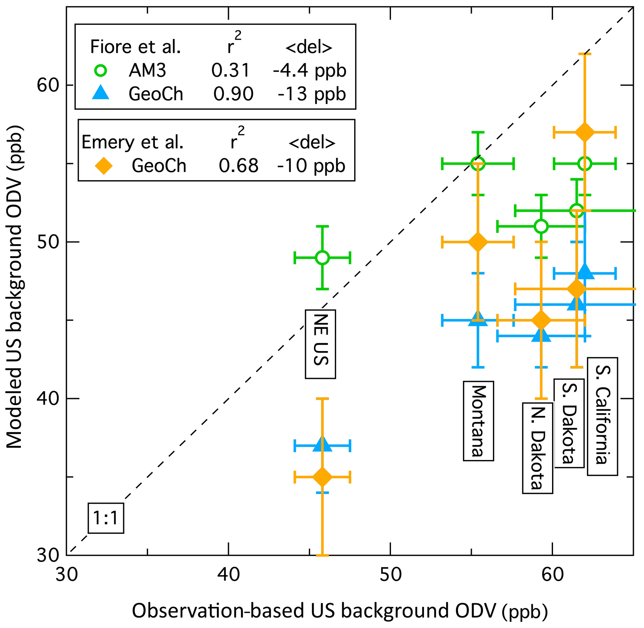
Figure 14Comparison of US background ODV estimates from model calculations with those derived in this work from observations. The r2 values of the correlations and the average differences (< del >) are annotated.
4.3 Possible shortcomings of the analysis
An uncertainty in the fits of the ODV time series to the exponential decay of the ODV enhancement term in Eq. (1) is the determination of the time constant, τ. The clear decrease in ODVs across the entire northeastern US did not begin until about 2000; the 18-year period of consistent decreases is not long enough for fits of Eq. (1) to accurately derive all three parameters. The primary approach we have taken is to use τ=21.9 years, the value determined for southern California (Parrish et al., 2017a) and in the northeastern US as well. It is not clear how the timescales of reductions in US anthropogenic ODV enhancements compare between California and the northeastern US. In California, precursor emission reductions may have been faster because that state may have had more aggressive emission control measures, but they may also have been slower because controls on eastern coal-fired power plants dramatically reduced NOx emissions. This latter reduction would not have occurred in California, where such power plants are located downwind and out of state. On the other hand, emission reduction rates could be roughly the same, as most northeastern US states have adopted the California on-road light-duty motor vehicle emission control program, and this is a large source sector both in California and the northeast. The alternative analysis approaches described in Sect. 2.3 with results discussed in Sect. 3.3 do not show evidence for a different exponential rate of decrease in US anthropogenic ODV enhancements between southern California and the northeastern states, but uncertainty in the value of τ remains a source of uncertainty in all of the results. The y0 and A values derived from the fits are sensitive to the selected τ value, with a larger value of τ attributing a smaller fraction of the ODV time series to y0 and yielding a larger A value.
Finally, Eq. (1) implicitly assumes that all sectors of anthropogenic US ozone precursor emissions have been reduced by emission controls at approximately the same rate. However, in some respects this is a poor approximation in that some emission sectors have received less effort than others. Any emissions that have not been reduced would tend to lead to an overestimate in the US background ODV, since ozone produced from those emissions would not have decreased. For example, Parrish et al. (2017a) note that continuing agricultural emissions in the Salton Sea Air Basin may account for the anomalously high y0 value derived for that region. Here, the possible influence of volatile chemical products (McDonald et al., 2018) in the northeastern US is mentioned above. It is not possible to account for uncertainties in the results that may arise from this issue.
4.4 Needs for further research efforts
Accurately quantifying the US background contribution to ODVs (i.e., the limit to which ODVs can be reduced through US anthropogenic emission reductions alone) is important from the perspective of determining the extent of emission reductions required to attain the ozone NAAQS. In this work we have determined the value of the parameter y0 of Eq. (1) within relatively small uncertainties (estimated 95 % confidence limits of ∼3 ppb). These uncertainties are derived from the scatter in the observed ODVs about the fits to Eq. (1). However, identifying the value of y0 as the US background ODVs brings in additional possible uncertainties (see discussion in the preceding section) that have not been quantified. Traditionally, models have been used to estimate US background ozone (see Jaffe et al., 2018, and references therein), but the models utilized in these efforts have significant shortcomings (e.g., see discussion in Parrish et al., 2017a) that lead to large uncertainties in the results. Jaffe et al. (2018) estimate an uncertainty in modeled seasonal mean US background ozone of about ±10 ppb, with greater uncertainty for individual days (such as those that define the ODV), and Guo et al. (2018) find biases as high as 19 ppb in modeled seasonal mean MDA8 ozone. Thus, modeling and the observationally based approach discussed in this paper are both available for estimating US background ODVs, but each has significant, poorly quantified uncertainties.
In summary, effective air quality management can be usefully informed by quantification of US background ODVs. However, given the relatively small differences between estimated US background ODVs and the 2015 ozone NAAQS of 70 ppb, these quantifications will be of more utility if they are accurate to within a couple of parts per billion (see Fig. 11 and associated discussion). Currently, two general approaches are available for estimating US background ODVs (the observationally based method discussed here and in Parrish et al., 2017a, and a variety of modeling approaches), but the limited comparisons of results from these two approaches and between the different model results indicate differences much larger than ideal. However, the magnitudes of these disagreements are within the uncertainty of the model estimates as discussed by Jaffe et al. (2018) and Guo et al. (2018). Further improvement is required in modeling systems until their output can accurately reproduce the magnitude and variability in the time series of observed ODVs discussed here; these model calculations could then provide accurate determination of the US background ODVs, the ODV enhancements from US anthropogenic emissions, and robust interpretations of the parameters y0 and A derived in this work. Until that model improvement is accomplished, the observationally based approach utilized in this work can provide useful estimates for air quality management guidance as well as for comparison with evolving model calculations.
All data used in this work are available from EPA's Air Quality System (AQS) data archive (https://www.epa.gov/aqs, last access: 23 June 2019).
The supplement related to this article is available online at: https://doi.org/10.5194/acp-19-12587-2019-supplement.
DDP conducted the analysis. CAE and DDP collaborated in writing the paper and responding to reviewers' comments.
The authors declare that they have no conflict of interest. David D. Parrish is the sole proprietor of David.D.Parrish, LLC, which has had contracts funded by several state and federal agencies and private companies. One of those contracts funded some of this work.
Some of the content of this paper was originally developed as a report submitted in fulfillment of the Technical Services Agreement between the Northeast States for Coordinated Air Use Management (NESCAUM) and David.D.Parrish. NYSERDA has not reviewed the information contained herein, and the opinions expressed in this report do not necessarily reflect those of NYSERDA or the state of New York. The authors appreciate the comments and discussion provided by Paul Miller of NESCAUM and Tom Ryerson, Fred Fehsenfeld, Owen Cooper, and Andrew Langford of NOAA/ESRL CSD. This paper has greatly benefited from extensive efforts of six anonymous referees and the editor. The scientific results and conclusions, as well as any views or opinions expressed herein, are those of the authors and do not necessarily reflect the views of NESCAUM, NOAA, or the Department of Commerce.
This research has been supported by the New York State Energy Research and Development Authority (NYSERDA; agreement no. 101132) and the National Oceanic and Atmospheric Administration (Atmospheric Chemistry, Carbon Cycle, and Climate – AC4 – Program).
This paper was edited by Ulrich Pöschl and reviewed by six anonymous referees.
Aleksic, N., Ku, J.-Y., and Sedefian, L.: Effects of the NOx SIP Call program on ozone levels in New York, J. Air Waste Manage., 63, 1335–1342, 2013.
Berger, R. E., Ramaswami, R., Solomon, C. G., and Drazen, J. M.: Air pollution still kills, New. Engl. J. Med., 376, 2591–2592, 2017.
Di, Q., Wang, Y., Zanobetti, A., Wang, Y., Koutrakis, P., Choirat, C., Dominici, F., and Schwartz, J. D.: Air Pollution and Mortality in the Medicare Population, New. Engl. J. Med., 386, 2513–2522, 2017.
Dolwick, P., Akhtar, F., Baker, K. R., Possiel, N., Simon, H., and Tonnesen, G.: Comparison of background ozone estimates over the western United States based on two separate model methodologies, Atmos. Environ., 109, 282–296, https://doi.org/10.1016/j.atmosenv.2015.01.005, 2015.
Emery, C., Jung, J., Downey, N., Johnson, J., Jimenez, M., Yarwood, G., and Morris, R.: Regional and global modeling estimates of policy relevant background ozone over the United States, Atmos. Environ., 47, 206–217, https://doi.org/10.1016/j.atmosenv.2011.11.012, 2012.
Fiore, A. M., West, J. J., Horowitz, L. W., Naik, V., and Schwarzkopf, M. D.: Characterizing the tropospheric ozone response to methane emission controls and the benefits to climate and air quality, J. Geophys. Res., 113, D08307, https://doi.org/10.1029/2007JD009162, 2008.
Fiore, A. M., Oberman, J., Lin, M., Zhang, L., Clifton, O. E., Jacob, D. J., Naik, V., Horowitz, L. M., Pinto, J. P., and Milly, G. P.: Estimating North American background ozone in U.S. surface air with two independent global models: Variability, uncertainties, and recommendations, Atmos. Environ., 96, 284–300, https://doi.org/10.1016/j.atmosenv.2014.07.045, 2014.
Fiore, A. M., Naik, V., and Leibensperger, E. M.: Air Quality and Climate Connections, J. Air Waste Manage., 65, 645–685, https://doi.org/10.1080/10962247.2015.1040526, 2015.
Guo, J. J., Fiore, A. M., Murray, L. T., Jaffe, D. A., Schnell, J. L., Moore, C. T., and Milly, G. P.: Average versus high surface ozone levels over the continental USA: model bias, background influences, and interannual variability, Atmos. Chem. Phys., 18, 12123–12140, https://doi.org/10.5194/acp-18-12123-2018, 2018.
Jacob, D. J., Logan, J. A., and Murti, P. P.: Effect of rising Asian emissions on surface ozone in the United States, Geophys. Res. Lett., 26, 2175–2178, https://doi.org/10.1029/1999gl900450, 1999.
Jaffe, D., Chand, D., Hafner, W., Westerling, A., and Spracklen, D.: Influence of fires on ozone concentrations in the western US, Environ. Sci. Technol., 42, 5885–5891, https://doi.org/10.1021/es800084k, 2008.
Jaffe, D., Wigder, N., Downey, N., Pfister, G., Boynard, A., and Reid, S. B.: Impact of Wildfires on Ozone Exceptional Events in the Western US, Environ. Sci. Technol., 47, 11065–11072, https://doi.org/10.1021/es402164f, 2013.
Jaffe, D. A., Cooper, O. R., Fiore, A. M., Henderson, B. H., Tonneson, G. S., Russell, A. G., Henze, D. K., Langford, A. O., Lin, M., and Moore, T.: Scientific assessment of background ozone over the U.S.: Implications for air quality management, Elem. Sci. Anth., 6, 56, https://doi.org/10.1525/elementa.309, 2018.
Langford, A. O., Aikin, K. C., Eubank, C. S., and Williams, E. J.: Stratospheric contribution to high surface ozone in Colorado during springtime, Geophys. Res. Lett., 36, L12801, https://doi.org/10.1029/2009gl038367, 2009.
Langford, A. O., Senff, C., Alvarez II, R., Brioude, J., Cooper, O., Holloway, J., Lin, M., Marchbanks, R., Pierce, R., Sandberg, S., Weickmann, A., and Williams, E.: An overview of the 2013 Las Vegas Ozone Study (LVOS): Impact of stratospheric intrusions and long-range transport on surface air quality, Atmos. Environ., 109, 305–322, https://doi.org/10.1016/j.atmosenv.2014.08.040, 2014.
Lin, M., Fiore, A. M., Cooper, O. R., Horowitz, L. W., Langford, A. O., Levy, H., Johnson, B. J., Naik, V., Oltmans, S. J., and Senff, C. J.: Springtime high surface ozone events over the western United States: Quantifying the role of stratospheric intrusions, J. Geophys. Res., 117, D00V22, https://doi.org/10.1029/2012jd018151, 2012a.
Lin, M., Fiore, A. M., Horowitz, L. W., Cooper, O. R., Naik, V., Holloway, J., Johnson, B. J., Middlebrook, A. M., Oltmans, S. J., Pollack, I. B., Ryerson, T. B., Warner, J. X., Wiedinmyer, C., Wilson, J., and Wyman, B.: Transport of Asian ozone pollution into surface air over the western United States in spring, J. Geophys. Res., 117, D00V07, https://doi.org/10.1029/2011jd016961, 2012b.
Lin, M., Fiore, A. M., Horowitz, L. W., Langford, A. O., Oltmans, S. J., Tarasick, D., and Rieder, H. E.: Climate variability modulates western US ozone air quality in spring via deep stratospheric intrusions, Nat. Commun., 6, 7105, https://doi.org/10.1038/ncomms8105, 2015.
Lin, M., Horowitz, L. W., Payton, R., Fiore, A. M., and Tonnesen, G.: US surface ozone trends and extremes from 1980 to 2014: quantifying the roles of rising Asian emissions, domestic controls, wildfires, and climate, Atmos. Chem. Phys., 17, 2943–2970, https://doi.org/10.5194/acp-17-2943-2017, 2017.
McDonald, B. C., de Gouw, J. A., Gilman, J. B., Jathar, S. H., Akherati, A., Cappa, C. D., Jimenez, J. L., Lee-Taylor, J., Hayes, P. L., McKeen, S. A., Cui, Y. Y., Kim, S.-W., Gentner, D. R., Isaacman-VanWertz, G., Goldstein, A. H., Harley, R. A., Frost, G. J., Roberts, J. M., Ryerson, T. B., and Trainer, M.: Volatile chemical products emerging as largest petrochemical source of urban organic emissions, Science, 359, 760–764, 2018.
McKeen, S. A., Wotawa, G., Parrish, D. D., Holloway, J. S., Buhr, M. P., Hübler, G., Fehsenfeld, F. C., and Meagher, J. F.: Ozone production from Canadian wildfires during June and July of 1995, J. Geophys. Res., 107, ACH 7-1–ACH 7-25, https://doi.org/10.1029/2001JD000697, 2002.
National Research Council (NRC): Rethinking the Ozone Problem in Urban and Regional Air Pollution, National Academy Press, Washington, DC, 1991.
Parrish, D. D. and Stockwell, W. R.: Urbanization and air pollution: Then and now, Eos: Earth & Space Science News, 96, 10–15, 2015.
Parrish, D. D., Fahey, D. W., Williams, E. J., Liu, S. C., Trainer, M., Murphy, P. C., Albritton, D. L., and Fehsenfeld, F. C.: Background Ozone and Anthropogenic Ozone Enhancement at Niwot Ridge, Colorado, J. Atmos. Chem., 4, 63–80, 1986.
Parrish, D. D., Young, L. M., Newman, M. H., Aikin, K. C., and Ryerson, T. B.: Ozone Design Values in Southern California's Air Basins: Temporal Evolution and U.S. Background Contribution, J. Geophys. Res.-Atmos., 122, 11166–11182, https://doi.org/10.1002/2016JD026329, 2017a.
Parrish, D. D., Petropavlovskikh, I., and Oltmans, S. J.: Reversal of long-term trend in baseline ozone concentrations at the North American West Coast, Geophys. Res. Lett., 44, 10675–10681, https://doi.org/10.1002/2017GL074960, 2017b.
Pfister, G. G., Wiedinmyer, C., and Emmons, L. K.: Impacts of the fall 2007 California wildfires on surface ozone: Integrating local observations with global model simulations, Geophys. Res. Lett., 35, L19814, https://doi.org/10.1029/2008GL034747, 2008.
Shen, L. and Mickley, L. J.: Effects of El Niño on summertime ozone air quality in the eastern United States, Geophys. Res. Lett., 44, 12543–12550, https://doi.org/10.1002/2017GL076150, 2017.
Shen, L., Mickley, L. J., Leibensperger, E. M., and Li, M.: Strong dependence of U.S. summertime air quality on the decadal variability of Atlantic sea surface temperatures, Geophys. Res. Lett., 44, 12527–12535, https://doi.org/10.1002/2017GL075905, 2017.
Turner, M. C., Jerrett, M., Pope III, C. A., Krewski, D., Gapstur, S. M., Diver, W. R., Beckerman, B. S., Marshall, J. D., Su, J., Crouse, D. L., and Burnett, R. T.: Long-Term Ozone Exposure and Mortality in a Large Prospective Study, Am. J. Resp. Crit. Care, 193, 1134–1142, 2016.
Wang, Y., Jia, B., Wang, S.-C., Estes, M., Shen, L., and Xie, Y.: Influence of the Bermuda High on interannual variability of summertime ozone in the Houston–Galveston–Brazoria region, Atmos. Chem. Phys., 16, 15265–15276, https://doi.org/10.5194/acp-16-15265-2016, 2016.
Wilcox, G. L.: New England and the Challenge of Interstate Ozone Pollution Under the Clean Air Act of 1990, B.C. Envtl. Aff. L. Rev., 24, 1–101, http://lawdigitalcommons.bc.edu/ealr/vol24/iss1/2 (last access: 2 October 2019), 1996.
Wolff, G. T. and Lioy, P. J.: Development of an ozone river associated with synoptic scale episodes in the eastern United States, Environ. Sci. Technol., 14, 1257–1260, 1980.