the Creative Commons Attribution 4.0 License.
the Creative Commons Attribution 4.0 License.
 | 08 Oct 2019
Microphysics of summer clouds in central West Antarctica simulated by the Polar Weather Research and Forecasting Model (WRF) and the Antarctic Mesoscale Prediction System (AMPS)
Keith M. Hines
David H. Bromwich
Sheng-Hung Wang
Israel Silber
Johannes Verlinde
Dan Lubin
The Atmospheric Radiation Measurement (ARM) West Antarctic Radiation Experiment (AWARE) provided a highly detailed set of remote-sensing and surface observations to study Antarctic clouds and surface energy balance, which have received much less attention than for the Arctic due to greater logistical challenges. Limited prior Antarctic cloud observations have slowed the progress of numerical weather prediction in this region. The AWARE observations from the West Antarctic Ice Sheet (WAIS) Divide during December 2015 and January 2016 are used to evaluate the operational forecasts of the Antarctic Mesoscale Prediction System (AMPS) and new simulations with the Polar Weather Research and Forecasting Model (WRF) 3.9.1. The Polar WRF 3.9.1 simulations are conducted with the WRF single-moment 5-class microphysics (WSM5C) used by the AMPS and with newer generation microphysics schemes. The AMPS simulates few liquid clouds during summer at the WAIS Divide, which is inconsistent with observations of frequent low-level liquid clouds. Polar WRF 3.9.1 simulations show that this result is a consequence of WSM5C. More advanced microphysics schemes simulate more cloud liquid water and produce stronger cloud radiative forcing, resulting in downward longwave and shortwave radiation at the surface more in agreement with observations. Similarly, increased cloud fraction is simulated with the more advanced microphysics schemes. All of the simulations, however, produce smaller net cloud fractions than observed. Ice water paths vary less between the simulations than liquid water paths. The colder and drier atmosphere driven by the Global Forecast System (GFS) initial and boundary conditions for AMPS forecasts produces lesser cloud amounts than the Polar WRF 3.9.1 simulations driven by ERA-Interim.


West Antarctica is among the most rapidly warming locations on Earth, and its warming is closely linked with global sea level rise (Rignot, 2008: Turner et al., 2006; Steig et al., 2009; Bromwich et al., 2013a, 2014). Recent paleoclimate work links temperature increases of a few degrees with past sea level increases of several meters due to disintegration of parts of the Antarctic Ice Sheet (DeConto and Pollard, 2016). Additional rise in Antarctic summer temperatures could lead to more frequent and extensive surface melting of the West Antarctic Ice Sheet (WAIS) (e.g., Nicolas and Bromwich, 2014). Conversely, increased temperatures can result in greater evaporation over the oceans and increased snowfall over Antarctica (Nicolas and Bromwich, 2014). The observational evidence shows West Antarctic warming since the 1950s (Bromwich et al., 2013a). Unlike the elevated ice mass of East Antarctica, West Antarctica is highly prone to intrusions of moist air from the Southern Ocean (Nicolas and Bromwich, 2011; Scott et al., 2017). Thus, the West Antarctic climate is much more ocean dominated than that of the colder and drier East Antarctica.
Moisture flux over West Antarctica leads to cloud formation. Clouds alter the net surface radiative flux and can thus impact the onset, extent, intensity, and duration of surface melting, refreezing, and ultimately meltwater control on cryospheric dynamics or runoff into the ocean (van Trincht et al., 2016). Modeling studies have shown that changes in cloud properties over Antarctica may impact regions of the globe well beyond high southern latitudes (Lubin et al., 1998). Moreover, Antarctic clouds have different characteristics than Arctic clouds (Hogan, 1986; Bromwich et al., 2012; Grosvenor et al., 2012; O'Shea et al., 2017). Silber et al. (2018a) show that cloud thickness at McMurdo Station peaks in austral winter, possibly due to cyclone activity, while Arctic cloud thickness peaks in boreal summer (Shupe, 2011). O'Shea et al. (2017) note significantly different types and concentrations of cloud condensation nuclei (CCN), and ice nuclei (IN) are expected between the Arctic and Antarctic due to the minimal anthropogenic sources at high southern latitudes. Aerosols tend to peak in winter and spring in the Arctic with a minimum during summer, while Antarctic aerosols tend to peak in austral summer and fall and are reduced during winter (e.g., Wagenbach et al., 1988; Schmeisser et al., 2018). Consequently, it is uncertain how well the findings of the various Arctic field programs and modeling experiments translate to Antarctica.
Clouds, including liquid water clouds, have a strong modulation on the local climate (Nicolas and Bromwich, 2011; Bromwich et al., 2012; Scott et al., 2017; Silber et al., 2018a). A supercooled liquid cloud is likely to be more optically thick than a fully glaciated ice cloud (Shupe and Intrieri, 2004; Grosvenor et al., 2012; McCoy et al., 2015). Arctic cloud modeling studies find that cloud liquid water is frequently underrepresented in simulations with bulk microphysics schemes, and this can result in too little longwave radiation and too much shortwave radiation reaching the surface (e.g., Morrison and Pinto, 2006).
Unfortunately, there have been few Antarctic field programs to detail cloud microphysical properties (e.g., Bromwich et al., 2012; Lachlan-Cope et al., 2016; Scott and Lubin, 2016). One study in the past decade by the British Antarctic Survey examined clouds over the Antarctic Peninsula (e.g., Grosvenor et al., 2012; Lachlan-Cope et al., 2016). Lachlan-Cope et al. (2016) found large differences in ice crystal concentrations between the clouds on the eastern and western sides of the peninsula, while Grosvenor et al. (2012) found elevated ice crystal concentrations with relatively warm temperature between −0.4 and −6.6 ∘C. They also found that several widely used IN parameterizations poorly represented the observed relationship between ice particle concentration and temperature. Accordingly, clouds are frequently poorly represented in numerical simulations for Antarctica (e.g., Bromwich et al., 2013b; King et al., 2015). The following sections discuss efforts to evaluate and improve the simulation of Antarctic clouds. The recent AWARE project is discussed in Sect. 2, while Sect. 3 describes the Polar WRF simulations for this project, including AMPS numerical weather prediction forecasts for Antarctica. Results are discussed in Sect. 4, and conclusions are given in Sect. 5.
The prime motivation for this work, as noted by Witze (2016), is that there has been little in-place atmospheric science or climatological field work over interior West Antarctica since 1967, when a weather balloon program ended. A few automatic weather stations there have provided direct meteorological information since 1980 (Lazzara et al., 2012). There is a need to quantify the impact of continental and oceanic air masses on the local hydrology and surface energy balance. Furthermore, there is a need for observations that can enable improved numerical simulations, both regional and global, through better representation of Antarctic clouds. The scarcity of cloud observations and well-tested simulations has so far inhibited significant progress. The work presented here may contribute to improvements to the AMPS simulations of clouds being sought by the National Center for Atmospheric Research (NCAR) if computational efficiency can be achieved (Jordan Powers, personal communication, 2018). Furthermore, we seek to evaluate and improve the numerical weather prediction for Antarctica, where the sparse observational network, the physics of the polar atmosphere, and the steep terrain challenge model capabilities (Bromwich et al., 2012). The need for accurate weather forecasting to support logistical and scientific activities has been important since the earliest Antarctic explorations
The Atmospheric Radiation Measurement (ARM) West Antarctic Radiation Experiment (AWARE, Witze, 2016) is a recent field program to study clouds and their impacts on atmospheric radiative transfer over the Antarctic continent. AWARE used the joint capabilities of the United States Antarctic Program, managed by the National Science Foundation, and the Department of Energy's second ARM Mobile Facility (AMF2) to provide quantitative data about energy components, changing air masses, and cloud microphysical data to improve model simulations of the ice sheet as influenced by Earth system processes. The AMF2 consists of a collection of lidars, radars, and radiometers taking remote-sensing observations of the Antarctic clouds combined with in situ instruments documenting the atmospheric state, but more comprehensive observations are needed.
Beginning late November 2015, AMF2 was deployed to Antarctica to make the most extensive suite of measurements in more than 40 years (Witze, 2016). The primary AWARE site was McMurdo Station (77.85∘ S, 166.72∘ E) at the southern tip of Antarctica's Ross Island, where observations took place between November 2015 and January 2017. A smaller suite of instruments was also deployed to the WAIS Divide (79.468∘ S, 112.086∘ W, 1803 m above sea level (a.s.l.)) for 47 d during the early and middle parts of austral summer (December 2015–January 2016).
The WAIS Divide component of the AWARE field campaign ran from 4 December 2015 through to 18 January 2016. A suite of ARM Mobile Facility instruments (Mather and Voyles, 2013) optimized for surface energy budget observations was moved from McMurdo to the WAIS Divide site during this period. Estimates of upper-air temperature and moisture were obtained from 6-hourly rawinsonde launches and continuous retrievals from a profiling microwave radiometer (MWR, Morris 2006). Liquid water path (LWP) was extracted from a co-location of the MWR with a G-Band Vapor Radiometer Profiler (Cadeddu, 2010). The uncertainty of observed LWP is 10 g m−2 (Cadeddu et al., 2009).
Upwelling shortwave and longwave radiative flux components were measured by a Surface Energy Balance System (SEBS, Cook, 2018). Downwelling flux components were measured by a Sky Radiation System, which consists of a normal incidence pyrheliometer, shaded pyranometers, and pyrgeometers (Dooraghi et al., 1996). The global downwelling shortwave flux was computed as in Nicolas et al. (2017). Surface fluxes for sensible and latent heat are derived according to the algorithm of Andreas et al. (2010). Near-surface measurements of temperature, moisture, and wind speed were measured by the ARM surface meteorological instrumentation (Holdridge and Kyrouac, 1993). Instruments at the WAIS Divide were unable to obtain reliable measurements of the heat flux within the ice pack. As an alternative, estimates of the conductive heat flux from the ice surface and the underlying ice were taken from Nicolas et al. (2017), who calculated the residual of other terms in the surface energy balance.
A cloud mask (derived from detected hydrometeor-bearing air volumes) is used to determine the cloud and liquid occurrence fractions at the WAIS Divide associated with the method of Silber et al. (2018a). In brief, depolarization micropulse lidar (MPL; Flynn et al., 2007) observations are used to generate a linear depolarization ratio (LDR) versus log-scaled particulate backscatter cross-section two-dimensional histogram that can identify the hydrometer categories (Silber et al., 2018b, c).
Hourly time series of total hydrometeor and liquid-cloud fractions were calculated from the processed cloud and liquid masks (with column integration). The occurrence fractions were normalized relative to the hourly MPL data availability, under the assumption that the measured period provided an acceptable representation of the whole hour. It should be noted that the MPL pulse can occasionally be completely attenuated by optically thick cloud layers (for example, as part of a frontal system). Therefore, the real cloud top, geometrical cloud thickness, and potentially the liquid occurrence are underestimated by the MPL in these situations.
The advanced research Weather Research and Forecasting Model (WRF) is an extensively used community numerical weather prediction model for numerous applications world-wide (e.g., Skamarock et al., 2008). Most of the polar optimizations for Polar WRF are added in the Noah land surface model (Barlage et al., 2010) and improve the representation of heat transfer through snow and ice (Hines and Bromwich, 2008; Hines et al., 2015). Fractional sea ice was implemented in Polar WRF by Bromwich et al. (2009), followed by the addition of specified variable sea ice thickness, snow depth on sea ice, and sea ice albedo. These updated options were developed by the Polar Meteorology Group (PMG) at Ohio State University's Byrd Polar and Climate Research Center and were included in the standard release of WRF (NCAR Mesoscale and Microscale Meteorology, 2019) with the help of the Mesoscale and Microscale Meteorology Division at NCAR (Hines et al., 2015). Hines et al. (2011) made comparisons for cloud and radiation quantities between Polar WRF 3.0.1.1 simulations and observations at the north slope of the Alaska ARM site.
Recently, Deb et al. (2016) evaluated Polar WRF 3.5.1 versus near-surface observations from West Antarctica. They found that pressure is simulated with high skill, and wind speed is generally well represented. The timing and amplitude of strong wind events were well captured. There were weaknesses in the diurnal cycle of temperature, especially denoted by a cold summertime minimum temperature bias. This was attributed to a negative bias in downwelling longwave radiation, consistent with clouds over Antarctica being poorly represented by models (e.g., Bromwich et al., 2012, 2013b; King et al., 2015; Listowski and Lachlan-Cope, 2017). Arctic modeling studies, however, suggest reason for optimism as Hines and Bromwich (2017) improved the representation of low-level liquid clouds by Polar WRF 3.7.1 with adjustments to the microphysics for simulations of the Arctic Summer Cloud Ocean Study (ASCOS, Tjernström et al., 2014) near the North Pole during the period August–September 2008.
3.1 AMPS
To improve forecasting support for the United States Antarctic Program, the National Science Foundation's Office of Polar Program initiated the Antarctic Mesoscale Prediction System (AMPS, Powers et al., 2012) in the year 2000. The AMPS is a real-time numerical weather prediction with Polar WRF through a collaboration between the National Center for Atmospheric Research (NCAR) and the PMG. The AMPS supports a variety of scientific and logistical needs for its international user base and has reduced costly flight turn-arounds between Christchurch, New Zealand, and the McMurdo Station (Powers et al., 2012).
For the time of the AWARE WAIS case study, the AMPS grid system consists of a series of nested domains with 60 vertical levels between the surface and the model top at 10 hPa. There are 12 layers in the lowest 1 km, with the levels nearest the surface at 10, 37, 73, and 119 m . The outermost domain had 30 km horizontal resolution and covered Antarctica and much of the Southern Ocean (Fig. 1a). Grid 2 had 10 km resolution and covered the Antarctic continent. Four additional higher-resolution nested domains (3.3 or 1.1 km) covered the Antarctic Peninsula, the South Pole and the region near the McMurdo Station. For the present study, grid 2 fields from the AMPS forecasts are used, and results are bilinearly interpolated to the WAIS Divide from the four nearest grid points. Sea ice fraction is provided by the National Snow and Ice Data Center analyses. The mesoscale representation in the initial fields is enhanced by the assimilation with 3-D variational data assimilation (Barker et al., 2004). Ingested fields include surface data, upper-air soundings, aircraft observations, geostationary and polar-orbiting satellite atmospheric motion vectors (AMVs), Constellation Observing System for Meteorology, Ionosphere, and Climate (COSMIC) GPS radio occultations, and Advanced Microwave Sounding Unit (AMSU) radiances. Twice daily AMPS forecasts are begun from analyses at 00:00 and 12:00 UTC of the Global Forecast System (GFS, NOAA Environmental Modeling Center, 2003), a global forecast system run by the U.S. National Centers for Environmental Prediction. For the current study we use the AMPS output for forecast hours 12–21 at 3 h intervals. Thus, our AMPS fields have a spin-up of a minimum of 12 h, with the possibility of jumps every 12 h due to the change toward a more recent initialization time. AMPS forecast fields in original WRF format are available from NCAR Mesoscale and Microscale Meteorology (2019). Selected AMPS output fields for March 2006–December 2016 for grids 2–6 can be downloaded from the Polar Meteorology Group (2017).
Figure 1Antarctic Mesoscale Prediction System (AMPS) grids (a) and grid for Polar WRF 3.9.1 simulations (b). The locations of McMurdo Station and the WAIS Divide are shown by triangles. Topography (m) is shown by color scales for both panels. Grid 2 in (a) with 10 km horizontal resolution is the same as the grid shown in (b). Grid 1 in (a) has 30 km resolution.
The scarcity of Antarctic meteorological observing stations and satellite blackout periods that can coincide with peak aircraft flight times increase the need for AMPS accuracy. Wille et al. (2017) note that unpredicted fog, low ceilings, and high winds lead to costly flight mission failures over Antarctica, thus accurately predicting acceptable flight windows is essential to prevent delays for science missions and cargo transportation. Unfortunately, the AMPS has been shown to underestimate low clouds over the Antarctica (Wille et al., 2017). According to Pon (2015) the cloud fraction product in the AMPS is so unreliable that most forecasters rely more on the AMPS relative humidity as a proxy for cloud predictions. Therefore, addressing the cloud prediction in the AMPS is a primary concern of this work.
Table 1Simulations for 3 December 2015 to 21 January 2016.
a Antarctic adaptations and data assimilation are included in the AMPS simulation. b The AMPS was upgraded from Polar WRF v. 3.3.1 to v. 3.7.1 on 19 January 2016.
The AMPS simulations used for the period 00:00 UTC 1 December 2015–12:00 UTC 19 January 2016 employ Polar WRF 3.3.1 as described by Wille et al. (2017). Afterward, the AMPS forecast system was upgraded to Polar WRF 3.7.1 (Table 1). The update has no impact on our analyses for the WAIS Divide, where all of the observations concluded prior to the change. Grid 2 at 10 km resolution has 667×628 horizontal grid points. The boundary layer is represented with the Mellor–Yamada–Janjić planetary boundary layer scheme with nonsingular implementation of level 2.5 Mellor–Yamada closure for turbulence in the planetary boundary layer and free atmosphere (Janjić, 1994). Cumulus is parameterized with the Kain–Fritsch scheme. The surface physics are represented with the 4-layer Noah land surface model with polar modifications (Bromwich et al., 2009; Hines et al., 2015). Other physics options include the Goddard shortwave radiation scheme (Chou et al., 2001), and the Rapid Radiative Transfer Model for GCMs (RRTMG, Clough et al., 2005) longwave radiation scheme. The WRF single-moment 5-class scheme (WSM5C, Hong et al., 2004) is employed to represent the cloud microphysics.
3.2 Polar WRF 3.9.1 simulations
Additional numerical simulations during the time of the AWARE field program are conducted with Polar WRF version 3.9.1 (Table 1). These are single-domain simulations with the same grid and topography as the AMPS grid 2 (Fig. 1b). The 60 vertical layers are identical to the AMPS simulations. In addition to the AMPS, prior simulations of Polar WRF guide the selection of physical parameterizations (e.g., Wilson et al., 2011, 2012; Bromwich et al., 2013b; Cassano et al., 2017; Hines and Bromwich, 2017). The Mellor–Yamada–Nakanishi–Niino (MYNN; Nakanishi and Niino, 2006) level-2.5 scheme is used for the atmospheric boundary layer and the corresponding atmospheric surface layer. We use RRTMG for longwave and shortwave radiation. Cloud liquid water, cloud ice, and snow impact the shortwave and longwave radiation, but rain water is not used in the radiation calculations. Cumulus is parameterized with the Kain–Fritsch scheme (Kain, 2004). The polar-optimized Noah land surface model is also used. The Polar WRF 3.9.1 simulations presented here input fractional sea ice concentrations from gridded fields at 12.5 km resolution processed by l'Institut Français de Recherche Pour l'Exploitation de La Mer (ftp://ftp.ifremer.fr/ifremer/, last access: 27 September 2019). The sea ice fraction for 12:00 UTC 10 January 2016 is shown in Fig. 2b. Sea ice albedo is set at 0.80, which is the same as the snow albedo.
Figure 2Plots of (a) simulated 2 m temperature (∘C, color scale), sea level pressure (contours, hPa), and 10 wind barbs (m s−1), and (b) represents sea ice fraction for 12:00 UTC 10 January 2016. Triangles are the locations of McMurdo Station and the WAIS Divide in (b).
One simulation, referred to as WRF GFS, is conducted with initial and boundary conditions taken from the GFS final analysis. The AMPS forecasts use the GFS forecasts by the same model which are available at the time. Thus, the AMPS and WRF GFS are conducted with the same forecast system, although the products used will not be identical. Additional observations are assimilated into the final analysis. Initial and boundary conditions of meteorological fields for the other Polar WRF 3.9.1 simulations are interpolated from ERA-Interim reanalysis (ERA-I; Dee et al., 2011) fields available every 6 h on 61 sigma levels and the surface at T255 resolution. We have made this change to obtain the best available agreement with observed clouds and radiation. Bracegirdle and Marshall (2012) found that, among the reanalyses they evaluated, ERA-I best represented the atmospheric circulation near Antarctica. Bromwich et al. (2013b) found that the boundary layer temperature fields were better represented in WRF simulations driven by ERA-I. Nudging toward analysis fields or observations is not performed on grid 2 during the forecast segment of the AMPS forecasts, and no nudging is included for the Polar WRF 3.9.1 simulations. Besides the microphysics schemes that are of interest to us, some differences between the AMPS and Polar WRF 3.9.1 simulations will occur due to the different base versions of WRF, the source for driving initial and boundary conditions, and the data assimilation used for AMPS initialization. Strict equality between the AMPS and Polar WRF simulations is not required for the goals of this paper, as we are interested in testing the sensitivity to the microphysics parameterization.
As shown in Table 1, four different schemes are employed for the cloud microphysics to see how the schemes impact the atmospheric hydrology and cloud radiative effect. Listowski and Lachlan-Cope (2017) previously tested five schemes with Polar WRF 3.5.1 for simulations over the central Antarctic Peninsula; however, we are interested in two newer schemes that have become available in more recent versions of WRF. Furthermore, the WAIS Divide is more southerly and colder, and the local atmosphere is likely to be more pristine than over the Antarctic Peninsula, where the oceanic influence is strong.
First, we consider WSM5C as it is the microphysics scheme used for the AMPS. This widely used scheme is computationally efficient and considers cloud water, cloud ice, rain, and snow as hydrometer classes. Cloud water and cloud ice are suspended, while rain and snow gradually precipitate out with a fall speed. Supercooled water is allowed to exist, and falling snow gradually melts at temperatures above 0 ∘C. Given that the AMPS simulations and the new Polar WRF 3.9.1 simulations are not conducted with identical model configurations, the simulation referred to as WSM5C (Table 1) is required for comparisons.
Three more recent schemes are also tested. Following Hines and Bromwich (2017), the two-moment Morrison scheme (e.g., Morrison et al., 2005, 2009) is used as it has been extensively tested in the Arctic and is known for its ability to simulate supercooled liquid water (e.g., Morrison et al., 2008; Klein et al., 2009; Solomon et al., 2011, 2014, 2015). It was amongst the best performing schemes in the simulations from Listowski and Lachlan-Cope (2017) . This two-moment bulk microphysics scheme predicts mixing ratios for cloud water, cloud ice, rain, snow, and graupel, and predicts number concentrations for cloud ice, snow, rain, and graupel. Particle size distributions are specified with gamma functions. The IN are parameterized according to the Cooper curve, with greater ice crystal concentrations at lower temperatures (Cooper, 1986). The prediction of two-moments (number concentration and condensate mixing ratio) allows a more robust treatment of the particle size distributions that are important for the microphysical process rates and cloud and precipitation evolution. The liquid water droplet concentration for clouds, however, is specified in the WRF implementation. The standard setting with WRF is 250 cm−3. Hines and Bromwich (2017) found the best results during the pristine ASCOS study in the Atlantic sector of the Arctic when the value was reduced to 20 cm−3 or less. For our AWARE simulations, we have selected 50 cm−3. The observations of Lachlan-Cope et al. (2016) and O'Shea et al. (2017) suggest liquid droplet concentrations are typically above 100 cm−3 for clouds over the Antarctic Peninsula and the Weddell Sea.
Simulations are also performed with the aerosol-aware Thompson microphysics scheme (Thompson and Eidhammer, 2014), which is an advance over the earlier Thompson et al. (2008) bulk microphysics scheme that was one-moment for cloud water and two-moment for cloud ice. This microphysics scheme accounts for cloud nucleating aerosol particles and five water species: cloud water, cloud ice, rain, snow, and graupel. The scheme includes 1st-order aerosol treatment with interactive IN and CCN concentrations. Nucleation or complete evaporation of hydrometeors deplete or add to condensation nuclei. Thus, the CCN process is now more interactive on a local scale. Cloud water, cloud ice, and rain are treated with two-moment predictions but snow with only single moment (mixing ratio) predictions. We refer to this scheme as the Thompson scheme. All cloud ice with diameters exceeding 200 µm are converted to snow, which tends to reduce cloud ice mixing ratios and ice particle diameters in comparison to other schemes (Greg Thompson, personal communication, 2017). Rather than using constant global values for CCN and IN that may be inappropriate for the polar regions, climatological values for CCN and IN are taken from a global dataset with spatial and monthly variability. The dataset is from a 7-year simulation of the Goddard Chemistry Aerosol Radiation and Transport (GOCART) model.
The final microphysics scheme is the Morrison–Milbrandt P3 scheme (Morrison and Milbrandt, 2015), hereafter called the P3 scheme. The use of the WRF 3.9.1 in our simulations is motivated by the addition of the very recent P3 scheme to the microphysics options. The new scheme avoids the previous arbitrary categorization of frozen hydrometers into cloud and precipitation, and thus allows for a continuum of particle properties. Fall speed is now applied across the continuum, rather than being limited to precipitation. There are four ice mixing ratio variables: total mass, rime mass, rime volume, and number, allowing for 4 degrees of freedom. Liquid hydrometers use a standard two-moment approach with cloud and rain categories. The constant liquid droplet number, 400 cm−3, is larger than the standard value for the Morrison scheme.
Both the P3 scheme and the Thompson scheme were unavailable in Polar WRF 3.5.1 when Listowski and Lachlan-Cope (2017) ran simulations for the Antarctic Peninsula. They tested the WSM5C, the WRF double-moment scheme, the Morrison scheme, the older Thompson scheme (Thompson et al., 2008), and the Milbrandt scheme (Milbrandt and Yau, 2005). The older Thompson scheme lacks the aerosol predictive ability of the newer Thompson scheme, and is single moment in cloud water. The last three schemes simulated clouds in best agreement with observations (Listowski and Lachlan-Cope, 2017). All schemes were unsuccessful in representing the supercooled water for some temperature ranges, but the results show that some schemes with more complicated microphysical parameterizations show improvements in representing Antarctic clouds.
The six simulations for this study are shown in Table 1. The AMPS 3 h output was retrieved for 1 December 2015 to 31 January 2016. Five Polar WRF 3.9.1 simulations were then performed. The AMPS has the same microphysics as the WSM5C and WRF GFS simulations. Unlike the AMPS forecasts, we used 24 hourly points of the Polar WRF 3.9.1 run segments. A 12 h spin-up is taken for each segment initialized at 00:00 UTC each day from 3 December 2015 to 19 January 2016. Output each hour for hours 12–35 is combined into fields spanning 12:00 UTC 3 December 2015 to 11:00 UTC January 2016. Polar WRF output is bilinearly interpolated from the four nearest grid points to the location of the WAIS Divide.
The time period of the December 2015–January 2016 field program at the WAIS Divide includes a major melting event over the Ross Ice Shelf and the adjacent Siple Coast of West Antarctica (Nicolas et al., 2017). Temperature over the Ross Ice Shelf and West Antarctica increased after 10 January, and many observing sites there experienced maximum temperatures above freezing for several days during the melting event. Figure 2a shows meteorological fields near the onset of the melting event, including the sea level pressure field, 2 m temperature, and 10 m wind speed from the WSM5C simulation at 12:00 UTC 10 January. Nicolas et al. (2017) discuss the contribution of a blocking high between 90 and 120∘ W to the melting event. Correspondingly, Fig. 2a displays anticyclonic shear for the wind barbs at this location. Northerly winds produce widespread advection of warm air over the Ross and Amundsen seas to the ice shelf and West Antarctica.
Figure 3Time series of (a) 2 m temperature (∘C) and (b) downwelling longwave radiation (W m−2) for the period 7–15 January 2016. The solid black curves show the observed temperature in (a) and the observed longwave radiation from Nicolas et al. (2017) in (b). The AMPS values are shown by dotted blue curves while dotted violet curves show the values from the Polar WRF 3.9.1 simulation with the WRF single-moment 5-class microphysics. The red curve shows the WRF GFS simulation.
4.1 Temperature and radiation
Time series of the 2 m temperature at the WAIS Divide for 7–15 January reveal large warming after 12:00 UTC 10 January (Fig. 3a). The observed temperature increases by 13.6 ∘C over 10 h after the minimum, then increases further to −1.4 ∘C at 18:00 UTC 11 January. Warmer locations at lower elevations over West Antarctica allow melting to occur (Nicolas et al., 2017). After a second peak of −1.8 ∘C late on 12 January, the WAIS Divide temperature gradually cools. The AMPS has a slight negative bias prior to the warming, then a negative bias of several degrees during the warm period that follows (Fig. 3a). Interestingly, the WSM5C simulation with Polar WRF 3.9.1 driven by ERA-I eliminates most of the negative bias prior to 10 January and during the warm period. The minimum temperature, however, drops to −22.4 ∘C at 08:00 UTC on 10 January in WSM5C. The simulation known as WRF GFS is frequently warmer than the AMPS for the time series shown in Fig. 3a but is usually colder than WSM5C during this time.
Table 2Model performance at WAIS for the period 4 December 2015–19 January 2016.a
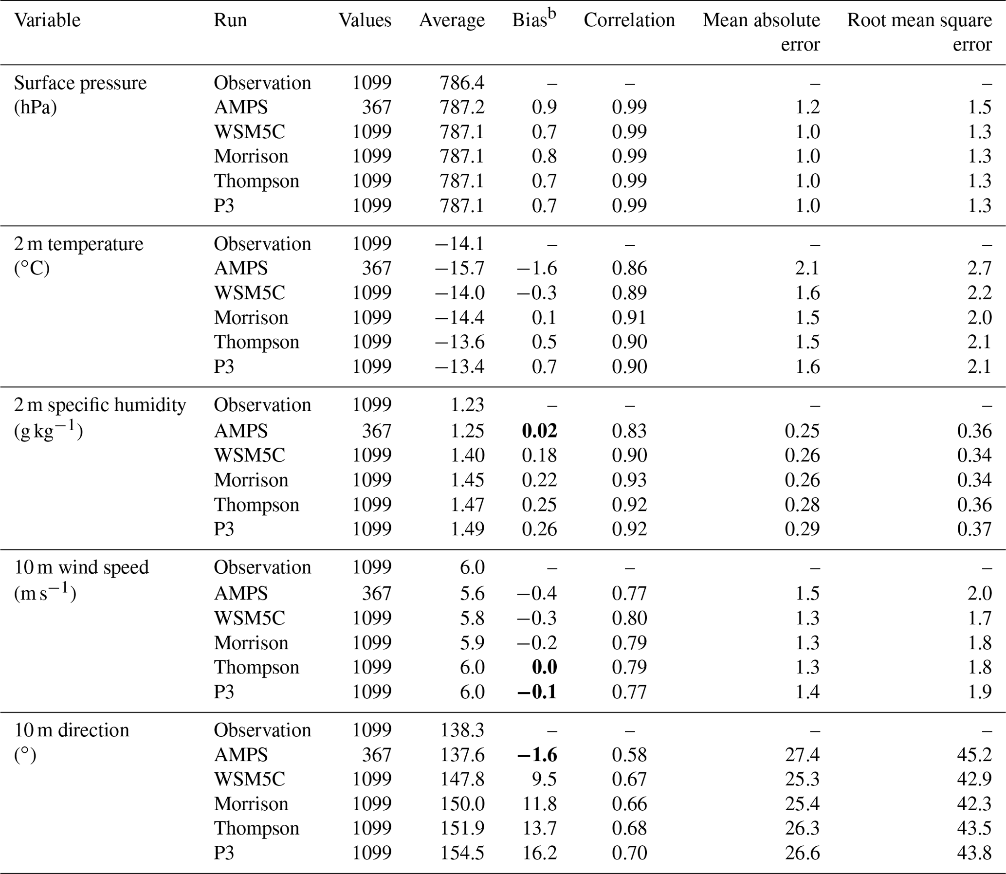
a Statistics are calculated from hourly values during the period 06:00 UTC 4 December
2015–00:00 UTC 19 January 2016 for the observations and the Polar WRF
3.9.1 runs. Values every 3 h are used for the AMPS results. Six values
are shown in each column for each variable. The values are for observations
(average only), the Antarctic Mesoscale Prediction System (AMPS), Polar WRF
3.9.1 simulation with the WRF single-moment 5-class microphysics (WSM5C),
Polar WRF 3.9.1 simulation with the Morrison microphysics (Morrison), Polar
WRF 3.9.1 simulation with the aerosol-aware Thompson microphysics
(Thompson), and Polar WRF 3.9.1 simulation with the Morrison–Milbrandt
microphysics (P3).
b All biases are statistically significant from zero at the 95 %
confidence level according to the Student's t test except for values shown
in bold. Most biases are also significant at the 99 % confidence level.
Table 2 shows statistics of simulations compared to observations. A total of 1099 hourly observations are available for most meteorological variables from 06:00 UTC on 4 December to 00:00 UTC on 19 January. Only values every 3 h are used for AMPS statistics, since output was available at these intervals, and means, biases and other statistics are impacted by the reduced number of values (367). For each variable, Table 2 shows observed averages, and the following rows show the AMPS, WSM5C, Morrison, Thompson, and P3 statistics. The largest magnitude temperature bias is for the AMPS, which has a negative bias of 1.6 ∘C during the observed period, and this appears in the time series shown in Fig. 3a. A negative bias is still present in WSM5C. However, it is reduced to 0.3 ∘C (Table 2). Both biases are statistically significant from zero at the 99 % confidence level according to the Student's t test. The bias for WRF GFS, −1.5 ∘C, is similar to that of the AMPS.
The reduced negative bias for WSM5C can be understood following the sensitivity tests by Bromwich et al. (2013b), with driving by the GFS final analysis (FNL) and ERA-I. They found the sensitivity to the source for initial and boundary conditions varied depending upon season and the choice of physical parameterizations. Their comparison using Polar WRF 3.2.1 with the MYNN planetary boundary layer and the RRTMG radiation scheme has the closest model configuration to that used for the AMPS and the Polar WRF 3.9.1 simulations. They found that the 2 m temperature bias changed from −3.3 to 0.1 ∘C with the switch from driving by FNL to driving by ERA-I (see their Table 5). Furthermore, the 2 m dew point bias increased from 1.2 to 4.0 ∘C.
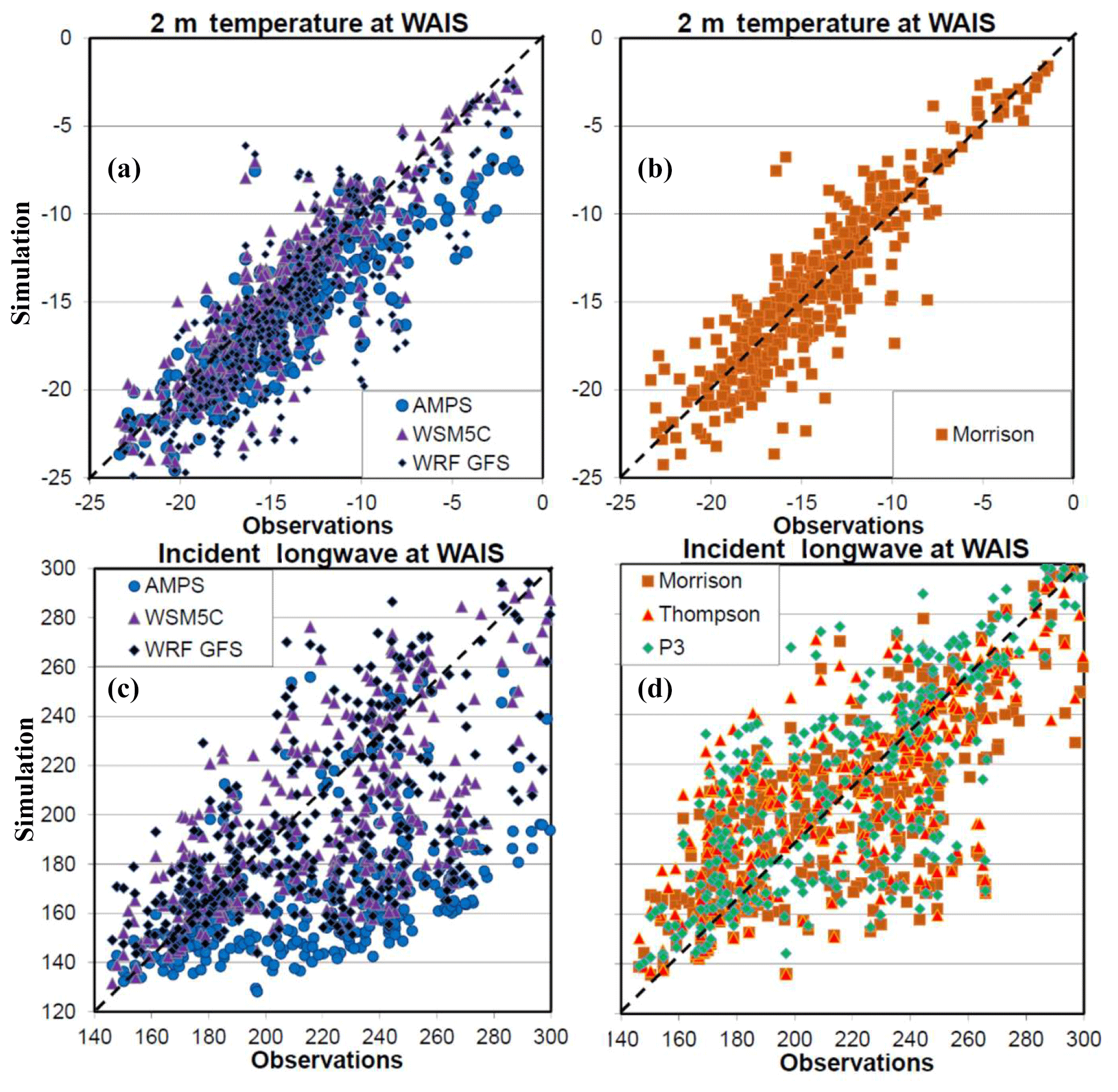
Figure 4Scatter plots of observed values (horizontal axis) and simulated results (vertical axis) of 2 m temperature (∘C) for (a) AMPS, WSM5C, and WRF GFS. (b) Morrison, and downwelling longwave radiation (W m−2) for (c) AMPS, WSM5C, and WRF GFS, and (d) Morrison, Thompson, and P3. The dashed line shows the 1:1 line.
Figure 4 shows scatter plots of the 2 m temperature and downwelling longwave radiation. The AMPS, WSM5C, and WRF GFS are shown in Fig. 4a. Morrison, Thompson, and P3 have similar scatter fields for the 2 m temperature; therefore only Morrison is shown (Fig. 4b). The cold bias for the AMPS is increased for temperature warmer than −8 ∘C. Therefore, the AMPS is unlikely to be able to properly represent West Antarctic melting events. Moreover, relatively warm events at the WAIS Divide are likely to be associated with cloud cover. This is consistent with Fig. 4c, as the error in downwelling longwave radiation is larger when the observed incident radiation at the surface is larger than 200 W m−2. In contrast, the Morrison simulation shows the simulated temperature to cluster around the one to one line over the entire range of observed temperature (Fig. 4b). Also, Morrison, Thompson, and P3 show less longwave error than the AMPS, WSM5C, and WRF GFS when the observed downwelling radiation is greater than 270 W m−2 (Fig. 4c and d).
The warmer and more moist atmosphere in the Polar WRF 3.9.1 simulations is demonstrated by vertical profiles of temperature and specific humidity biases compared to radiosonde observations (Fig. 5). There is a general negative bias except near 1900 m a.s.l., where the positive biases reach up to 0.8 to 0.9 ∘C (Fig. 5a). Thus, there is a weaker near-surface lapse in the simulations than the observations (not shown). The most extreme bias is the near-surface cold bias for the AMPS that reaches 2.3 ∘C. The cold bias for the AMPS is also larger than 1 ∘C between 3500 and 5100 m a.s.l.
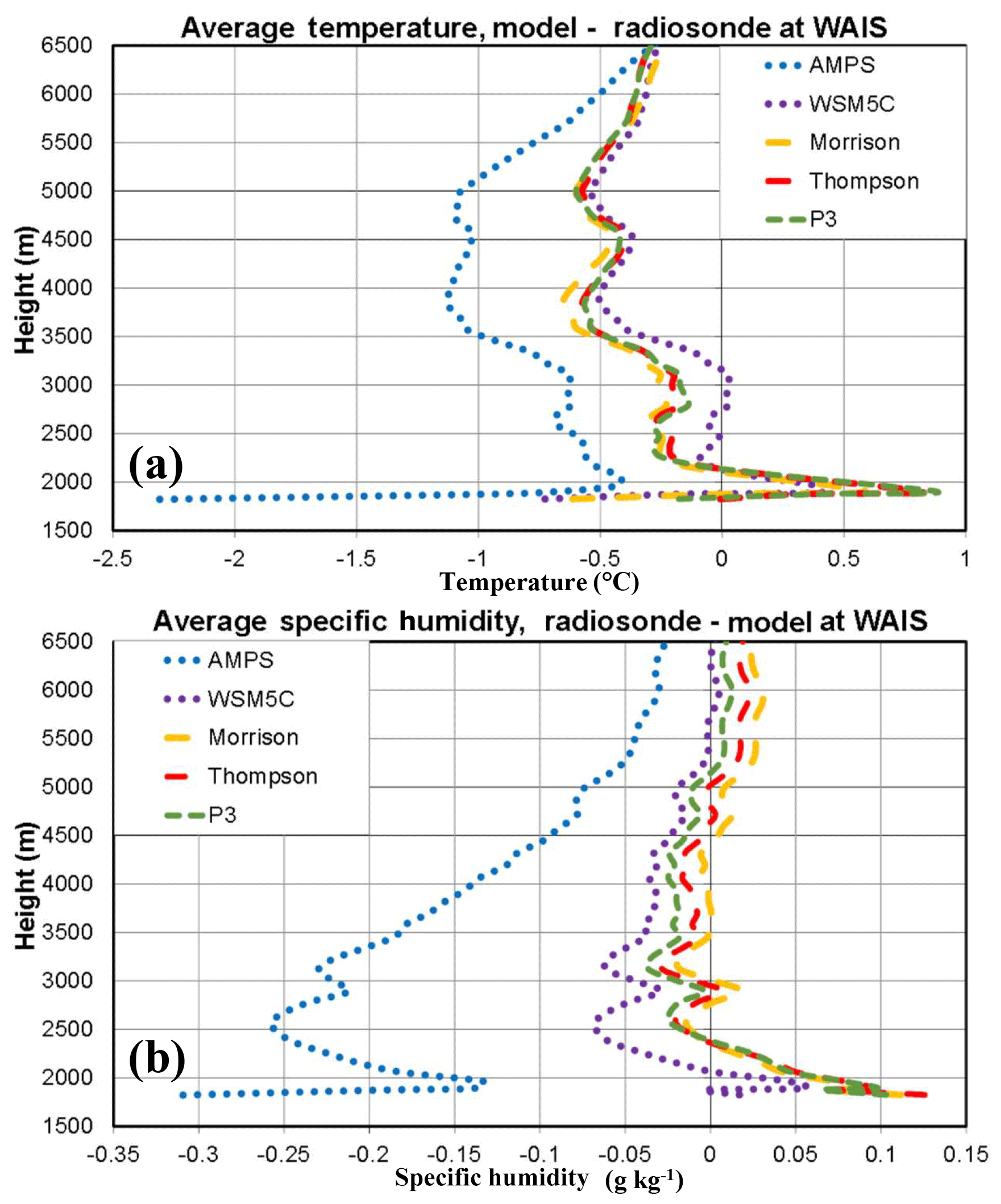
Figure 5Vertical profiles of average (a) temperature (∘C) and (b) specific humidity (g kg−1) differences between simulations and radiosonde observations from 2 to 16 January 2016.
An especially striking difference between the AMPS simulation forced with GFS and the simulations driven with ERA-I is shown in Fig. 5b. The AMPS is dryer than the radiosonde observations at the WAIS Divide at all levels shown, especially in the lowest 3000 m a.s.l. The WSM5C simulation is slightly drier than the other Polar WRF simulations. The simulations with the newer microphysics schemes are more moist than the observations just above the surface with biases as large as 0.13 g kg−1. Above the boundary layer, the specific humidity biases are small, generally below as 0.03 g kg−1, for the simulations with the newer microphysics. From Fig. 5, we can attribute the differences between the AMPS and WSM5C simulations to the colder and drier atmosphere initiated with GFS initial conditions for the AMPS.
Figures 3b and 6b help to explain the near-surface temperature results. Downwelling longwave radiation shows a clear negative bias for both the AMPS and WSM5C, but the magnitude is much larger for the former. Table 3, with contribution from SEBS observations for 7 December to 16 January, shows that the downwelling longwave bias is quite large, −41.5 W m−2 for the AMPS. The bias is reduced to −14.8 W m−2 for WSM5C and −17.0 W m−2 for WRF GFS. The WRF GFS simulation also has a slightly larger downwelling shortwave radiation bias, 22.3 W m−2, than the other Polar WRF 3.9.1 simulations. Since the WRF radiation biases for WRF GFS are not greatly different than those of the WSM5C simulation which has the same microphysics scheme, WRF GFS is not discussed further.

Figure 6Average diurnal cycles over 4 December 2015–19 January 2016 for (a) 2 m temperature (∘C) and (b–d) over 7 December 2015–16 January 2016 for surface radiation (W m−2). (b) Downwelling longwave radiation, (c) downwelling shortwave radiation, and (d) upwelling shortwave radiation. The error bars represent the 95 % confidence level for differences between sample averages according the t test (see text).
Table 3Surface energy balance at WAIS for the period 7 December 2015–16 January 2016.a
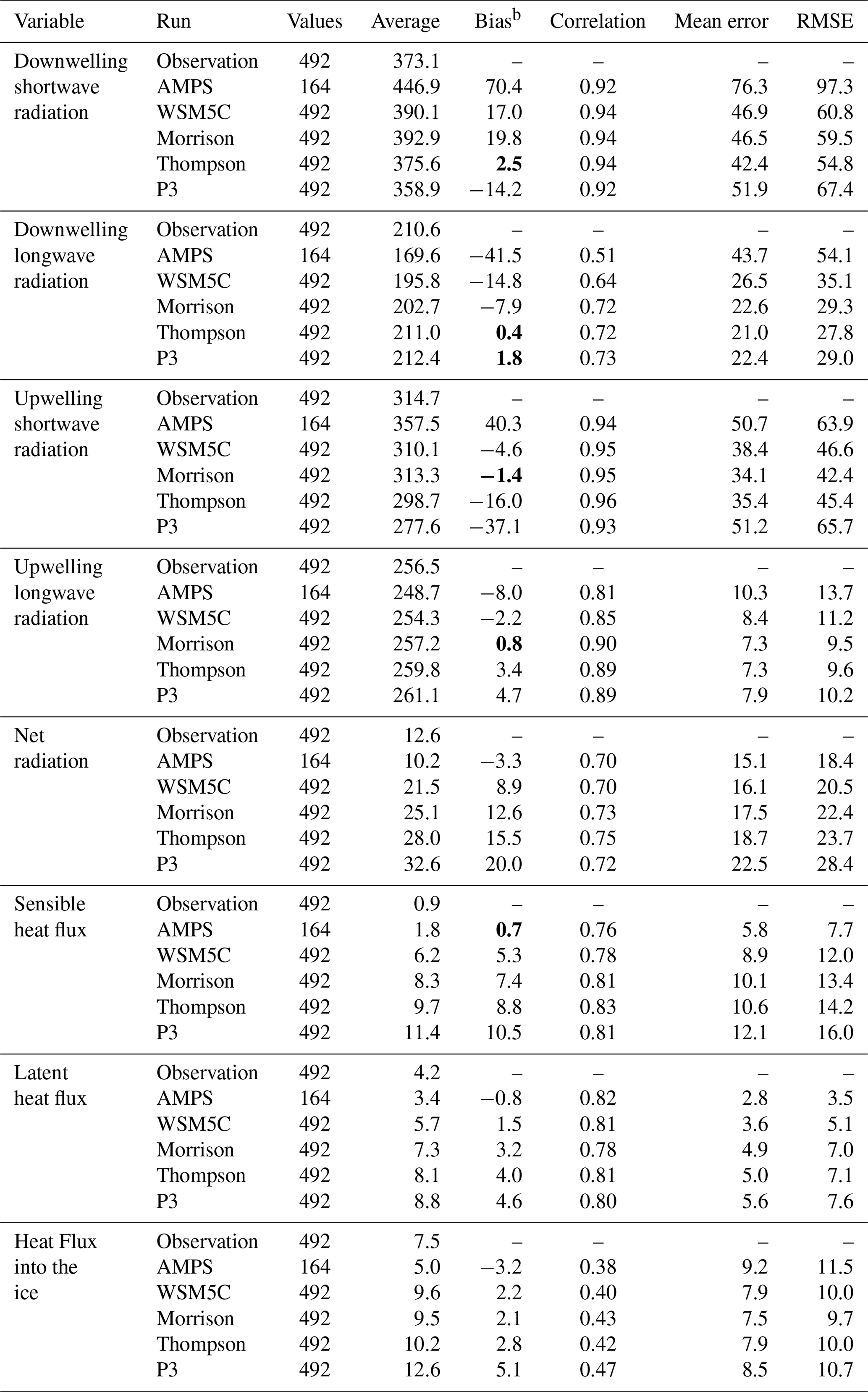
a Statistics are calculated from values every other hour during the period 01:00 UTC
7 December 2015–23:00 UTC 16 January 2016 for the observations and the Polar
WRF 3.9.1 runs. Values at 03:00, 09:00, 15:00, and 21:00 UTC are used for the AMPS
results. Six values are shown in each column for each variable. The values
are for observations (average only), AMPS, WSM5C, Morrison, Thompson, and P3.
b All biases are statistically significant from zero at the 95 %
confidence level according to the Student's t test, except for values shown
in bold. Most biases are also significant at the 99 % confidence level.
The deficit in longwave radiation is contributing to the negative temperature bias. Even though the downwelling shortwave biases are positive for the AMPS and WSM5C (Table 3), most of the solar flux is reflected by the ice surface. Thus, the net radiation flux bias is negative, −3.3 W m−2, for the AMPS. This is consistent with the greater impact of longwave cloud forcing than shortwave cloud forcing over Antarctica (Pavolonis and Key, 2003). Since a negative bias in downwelling longwave radiation and a positive bias for downwelling shortwave radiation are found for both the AMPS and WSM5C, we believe Polar WRF 3.9.1 simulations can be used to explore the cloud radiative biases that impact the AMPS forecasts and aim to seek improvements. Downwelling and upwelling longwave biases for both the AMPS and WSM5C are all statistically significant (Table 3).
Figure 6 shows the diurnal cycles of average fields for 2 m temperature, downwelling longwave radiation, downwelling shortwave radiation, and upwelling shortwave radiation. The time periods for averaging are 4 December 2015–19 January 2016 for the temperature and 7 December 2015–16 January 2016 for the radiation terms. Simulated biases in these fields vary with time of day, with local noon near 19:30 UTC. To provide an idea of the statistical significance of differences in Fig. 6a, we use the Student's t test for the AMPS and the observations. The observed temperature time series was adjusted each hour of the day by a constant value until the statistical significance of the model minus observed difference was at the boundary of the 95 % confidence level. Accounting for autocorrelation in the temperature time series, the degrees of freedom were reduced by a factor of 3. Accordingly, the bias at which the statistical confidence would be 95 % could be established. The error bars every 3 h in Fig. 6a show the range next to the observations for which differences are not statistically significant. Since AMPS values and observations of the surface energy balance are simultaneously available only four times a day, we use the WSM5C simulation and the observations to determine the statistical significance error bars for Fig. 6b–d (every 2 h beginning at 01:00 UTC).
The AMPS mean temperature in the daily cycle is less than the observed value at all AMPS output times. Only 03:00 UTC is not statistically significant. The observations have an earlier minimum of −16.0 ∘C at 07:00 UTC, while the AMPS minimum of −18.5 ∘C occurs at 12:00 UTC. The AMPS negative bias, peaks at 12:00 UTC (3.1 ∘C). For the Polar WRF 3.9.1 runs, WSM5C is close enough to the observations to be within statistical uncertainty for most hours, except near the time of minimum temperature, when there is a negative bias of 1–2 ∘C. The simulations with more advanced microphysics schemes are warmer than the observations during the hours of decreasing temperature. P3 is warmest during these times with statistically significant biases of 1.1 to 1.7 ∘C. The transition between run segments at 12:00 UTC results in a temperature decrease of up to 2 ∘C, but the change is much less for WSM5C. Starting at 15:00 UTC, the Polar WRF 3.9.1 simulations show small temperature biases that are not statistically significant. At, or just after, the time of maximum temperature, the Polar WRF 3.9.1 simulations show positive biases that are statistically significant for Morrison, Thompson, and P3. Obviously, the choice of microphysics scheme impacts the temperature bias at the WAIS Divide by enough to change the sign of the overall bias, and this is shown in Table 2 with positive biases of 0.1, 0.5, and 0.7 ∘C using the Morrison, Thompson, and P3 schemes, respectively.
For downwelling shortwave radiation (Fig. 6c), the AMPS has statistically significant positive biases at all hours, with the bias peaking at 106 W m−2 at 15:00 UTC. The bias is much reduced for the Polar WRF 3.9.1 simulations and not statistically significant at most observation times. The Morrison scheme, however, does show a statistically significant positive bias ahead of solar noon, while P3 shows a negative bias after solar noon. Figure 6d shows P3 to be an outlier for upwelling shortwave radiation near the hours of maximum insolation. Table 3 shows that the overall biases for all times during the observing period are 70.4, 17.0, 19.8, 2.5, and −14.2 W m−2 for AMPS, WSM5C, Morrison, Thompson, and P3, respectively. All these biases are statistically significant at the 99 % confidence level, except for the Thompson scheme for which the bias fails the 95 % confidence test.
The shortwave results are encouraging and suggest that changing the microphysics scheme can greatly alleviate and perhaps even reverse Antarctic radiation biases in numerical simulations. It may appear odd, however, that the upwelling shortwave radiation shows negative biases for all the Polar WRF 3.9.1 simulations that do not coincide with downwelling biases. The difference can be explained by the specified snow albedo in the WRF Noah routine. The specified maximum snow albedo is 0.8 for Noah, and average simulation albedos are slightly below this value. The average observed albedo, however, is 0.843. Therefore, a higher fraction of solar insolation is reflected at the WAIS Divide than in these simulations. This results in a deficit of upwelling shortwave radiation (Table 3, Fig. 6d). The deficit increases the net radiation and contributes to the positive temperature bias for the Morrison, Thompson, and P3. The impact of the albedo can be seen in the slope of the temperature curves after 12:00 UTC in Fig. 6a.
We ran a sensitivity test with segments initialized at 00:00 UTC each day between 6 and 16 January 2016. The active period for analysis is 12:00 UTC on 6 January until 11:00 UTC on 17 January. The settings were equal to the WSM5C; however, the albedo over glacial ice was increased to 0.84, closer to the observed albedo at the WAIS Divide. For the used part of the segments (hours 12–35), the 2 m temperature average was −12.4 ∘C in the sensitivity test. That is, 1.6 ∘C colder than WSM5C during the same period. That is almost twice the magnitude of the spread of the bias in Polar WRF 3.9.1 simulations shown in Table 2. We surmise that a more realistic surface albedo would likely result in a cold bias for the Polar WRF 3.9.1 simulations.
The observed downwelling longwave radiation (see Fig. 6b) has a mean value of 210.6 W m−2 (Table 3). The AMPS shows a strong negative bias at all hours that peaks at −53.0 W m−2 at 15:00 UTC. The magnitude of the bias is much reduced for WSM5C, but the deficit from the observations is statistically significant at the 95 % confidence level except at 03:00 and 05:00 UTC. The overall bias for all times is −14.8 W m−2 and is statistically significant at 99 % confidence (Table 3). While there is a large difference between the AMPS and WSM5C, the microphysics scheme is nevertheless associated with excess incoming shortwave radiation and a deficit in incoming longwave radiation. This is consistent with the WSM5C results over the Antarctic Peninsula reported by Listowski and Lachlan-Cope (2017). They also found that the Morrison scheme can alleviate radiation errors. Similarly, the radiation results were improved here with the Morrison, Thompson, and P3 schemes. While the WSM5C scheme lies outside the error bars at most hours, the other three schemes are within the error bars at most hours in Fig. 6b. Table 3 shows overall downwelling longwave biases of −7.9, 0.4, and 1.8 W m−2 for Morrison, Thompson and P3, respectively. The last two biases are not statistically significant from zero. Correspondingly, Fig. 6b shows that the three advanced schemes do not have statistically significant biases at most hours. The Morrison scheme, however, does show deficits exceeding 14 W m−2 at 13:00 and 15:00 UTC. These longwave and shortwave results suggest strengths and weaknesses in the simulation of Antarctic clouds.
4.2 Clouds
Figure 7 shows the average diurnal cycle over 7 December–17 January of longwave and shortwave cloud forcing at the surface for the simulations. Cloud forcing (CF) is defined following Eq. (1):
where Fall sky is the net all sky flux, and Fclear sky is the net clear-sky flux that is estimated to occur without the presence of clouds. Cloud forcing represents the warming effect of clouds (or cooling in the case of negative values) and can be calculated for the longwave, shortwave, or combined flux. Pavolonis and Key (2003) used 1985–1993 data including Advanced Very-High-Resolution Radiometer on NOAA polar orbiting satellites and the International Satellite Cloud Climatology Project to estimate cloud forcing. They found summertime shortwave cloud forcing of about −10 to −18 W m−2 for the latitude of the WAIS Divide. Longwave cloud forcing was 17–35 W m−2. For more recent estimates, Scott et al. (2017) used the Clouds and the Earth's Radiant Energy System (CERES) CALIPSO–CloudSat–CERES–MODIS dataset (Kato et al., 2011) to obtain monthly surface cloud forcing. From 2007 to 2010 satellite observations for points near the WAIS Divide, they found January values of 57.3, −29.1, and 28.3 W m−2 for longwave, shortwave, and net cloud forcing, respectively.

Figure 7Average diurnal cycles over 7 December 2015–16 January 2016 for (a) longwave cloud forcing (W m−2) and (b) shortwave cloud forcing (W m−2). AMPS values are shown in (a) as clear-sky values are available for longwave radiation; however, they are not available for shortwave radiation. Consequently, shortwave cloud forcing was not calculated for the AMPS.
Polar WRF 3.9.1 produced clear-sky flux values for longwave and shortwave radiation, so cloud forcing could be readily calculated. Clear-sky shortwave fluxes were not available from the AMPS. Figure 7a clearly shows that the longwave cloud forcing for the AMPS is weak, while the longwave cloud forcing for WSM5C is less than that of the more recent schemes. The results for the AMPS and WSM5C are consistent with the negative temperature biases during these simulations. P3 produces the greatest overall longwave cloud forcing, but the impact varies somewhat with time of day. Thompson produces nearly as much longwave cloud forcing as P3. The overall averages are 12.2, 31.9, 37.1, 44.8, and 46.1 W m−2 for AMPS, WSM5C, Morrison, Thompson, and P3, respectively. The simulated cloud forcing tends to be much greater than the climatological values of Pavolonis and Key (2003), yet smaller than the values reported by Scott et al. (2017). Given that clouds contributed to the major melting event during January 2016 (Nicolas et al., 2017), cloud forcing in excess of the climatological mean is possible for this month.
Figure 7b shows shortwave cloud forcing which has a cooling effect on the surface. There are considerable differences between the more recent microphysics schemes. The overall averages are −11.0, −10.1, −13.7, and −18.5 W m−2 for WSM5C, Morrison, Thompson, and P3, respectively. P3 shows a strong diurnal cycle with a minimum magnitude (−13.5 W m−2) at 08:00 UTC and a maximum magnitude (−25.2 W m−2) at 23:00 UTC near the time of maximum insolation and temperature. In contrast, Morrison shows a small diurnal variation. More recent microphysics schemes produce stronger cloud radiative properties than WSM5C. Of the recent schemes, P3 shows the strongest cloud radiative impact, while Morrison shows the least.
The average diurnal cycles of sensible heat flux and the conductive heat flux into the ice at the WAIS Divide are shown in Fig. 8. The conductive flux was not directly measured by Nicolas et al. (2017); however, the flux was estimated from the residual of other terms in the surface energy balance. The diurnal cycle of sensible heat flux was greatly amplified in the simulations compared to the observations (Fig. 8a). The positive sensible heat fluxes into the atmosphere are especially large near the time of maximum temperature, with a maximum of 32.3 W m−2 at 19:00 UTC for P3. The maximum is much smaller for the AMPS (15.3 W m−2), which is colder. The overall average observed value is small, 0.9 W m−2 (Table 3). Modeled overall averages vary from 1.8 W m−2 for the AMPS to 11.4 W m−2 for P3.
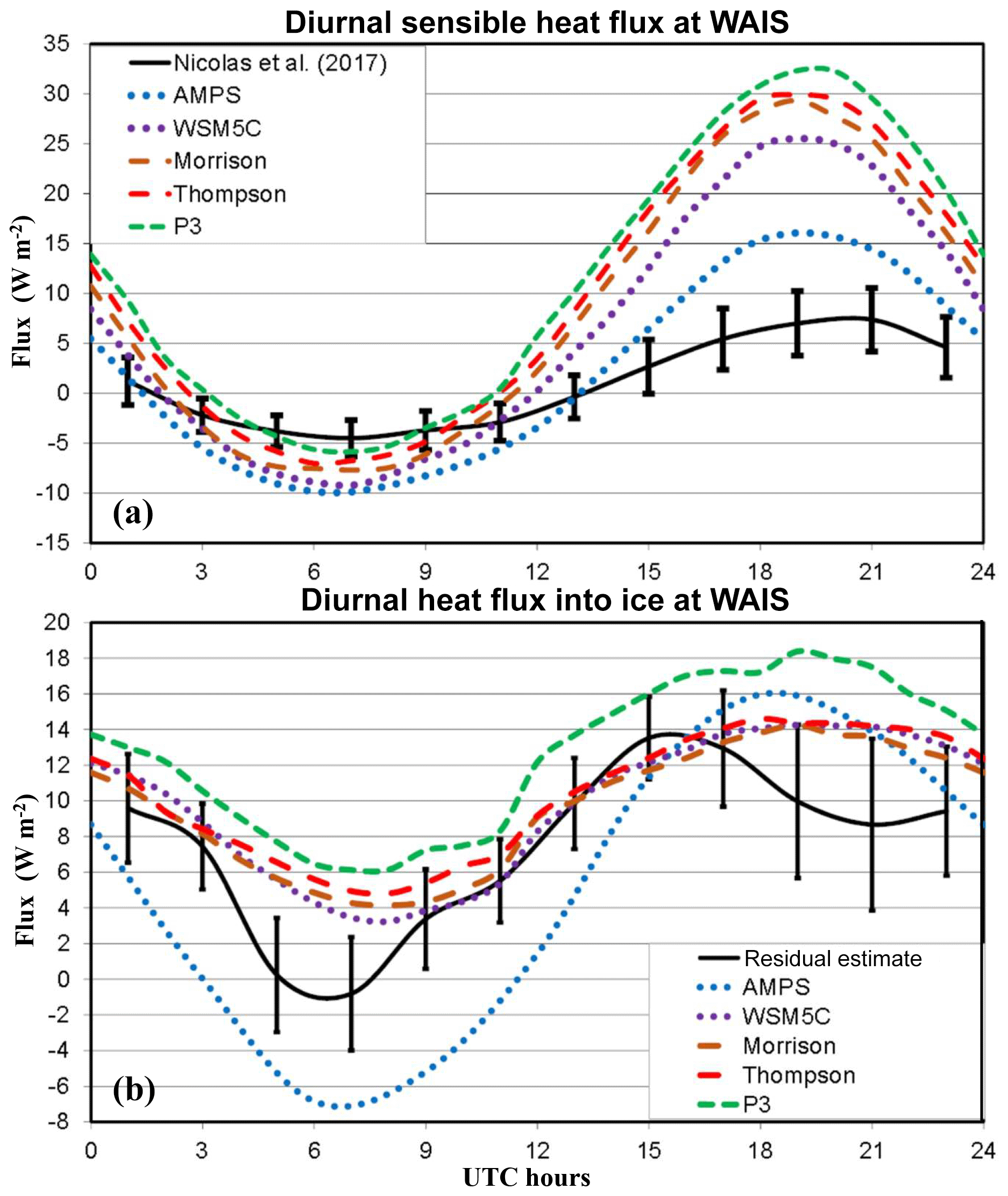
Figure 8Average diurnal cycles over 7 December 2015–16 January 2016 for (a) sensible heat flux (W m−2) and (b) heat flux into the ice pack (W m−2). The WAIS observations are available for (a), while an estimate of the heat flux for (b) is available from the residual of surface energy balance terms.
The conductive flux into the ice is a critical term for mass balance of West Antarctica. Therefore, it is important for modeling studies to be able to well represent this quantity. Positive values are expected during December and January when insolation is large. The overall average for the residual estimate of Nicolas et al. (2017) is 7.5 W m−2 during the observational period (Table 3). The AMPS, which has a negative temperature bias, also has a difference of −3.2 W m−2 compared to the estimated conductive flux of Nicolas et al. (2017). The overall biases are positive for all the Polar WRF 3.9.1 simulations, with values of 2.2, 2.1, 2.8, and 5.1 W m−2 for WSM5C, Morrison, Thompson, and P3, respectively. The large values during the warmer part of the day are key to the positive biases (Fig. 8b).

Figure 9Time series of (a, b) liquid water path (mm) and (c) ice water path (mm) from 00:00 UTC on 2 January to 00:00 UTC on 18 January 2016. Microwave radiometer (MWR) observations are available for liquid water path and are shown by solid curves in (a, b). Values for the AMPS and the WSM5C simulation are shown in (a, c), while values for the three simulations with advanced microphysics schemes are shown in (b, c).
While the previous analysis has concentrated on radiation fields and the surface energy balance, we now more directly examine the observed and simulated clouds. Figure 9 shows the LWP for the period 2–18 January 2016. Modeled LWP includes both suspended liquid cloud droplets and falling rain. LWP values above zero are observed at most times, but the AMPS and WSM5C simulate non-zero values only during the period 11–12 January (Fig. 9a). The results demonstrate the known difficulty of the WSM5C microphysics in simulating liquid water for polar clouds (e.g., Listowski and Lachlan-Cope, 2017). The more advanced microphysics schemes simulate liquid water much more frequently than WSM5C but do not well represent the instantaneous observed liquid water (Fig. 9b). Therefore, we suggest that the simulation of liquid water in polar clouds remains problematic (e.g., King et al., 2015; Hines and Bromwich, 2017; Listowski and Lachlan-Cope, 2017).
Table 4 shows the average condensate from 00:00 UTC on 2 January to 00:00 UTC on 18 January. The average observed LWP, 23 g m−2, is larger than in any of the simulations. The largest simulated value is 15.5 g m−2 for P3, which is consistent with magnitude of cloud forcing for this simulation (Fig. 7). Morrison has a smaller LWP value, 5.1 g m−2, than Thompson or P3, which corresponds to the weaker cloud forcing in Fig. 7. The LWP values are small, 0.43 and 0.88 g m−2 for the AMPS and WSM5C, respectively. The radiative impact of microphysics schemes for the WAIS appears to be strongly linked to the ability to simulate liquid water.
Table 4Mean hydrometers (g m−2) at the WAIS for the period 2–18 January 2016.
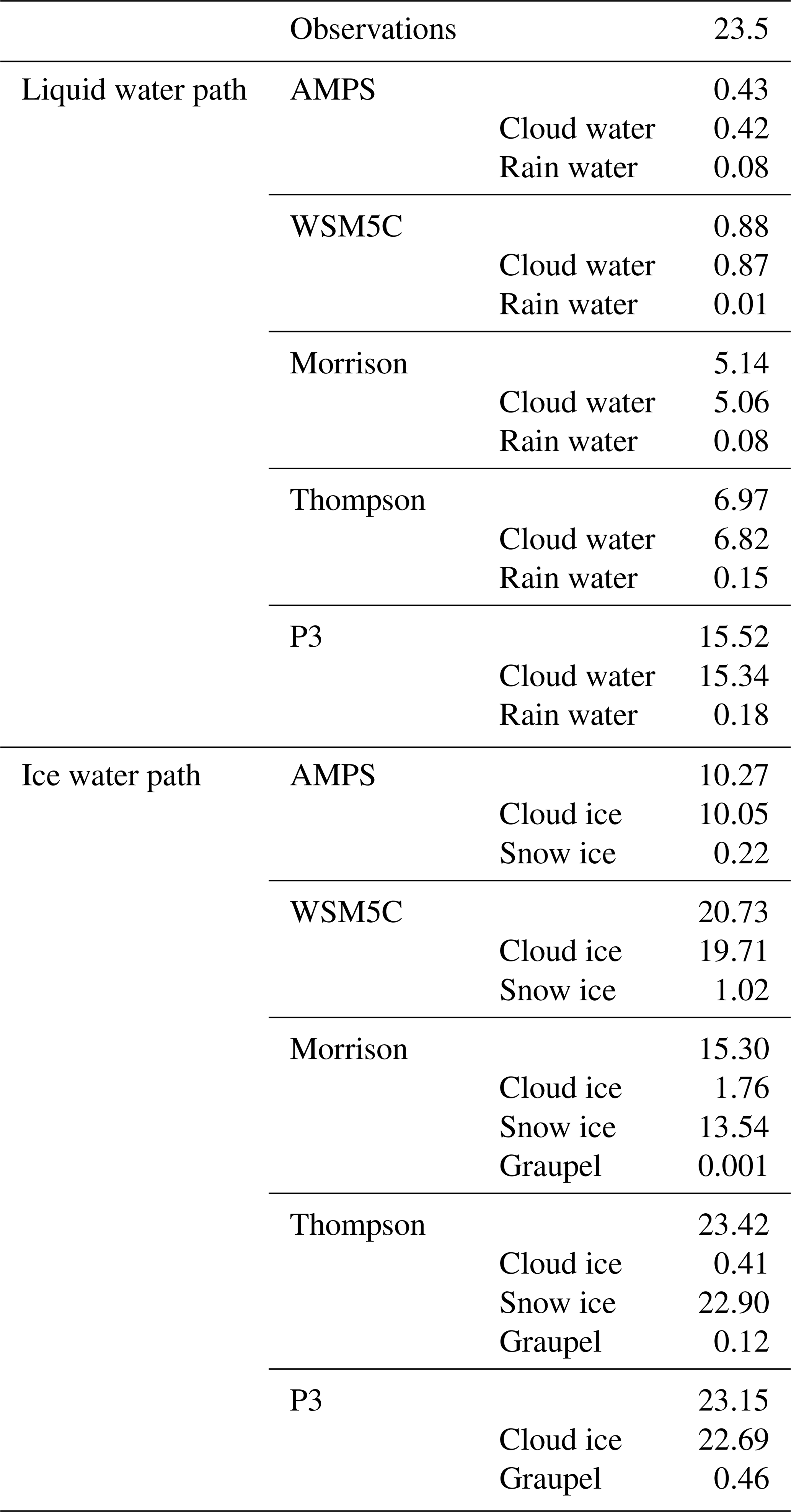
Caution should be applied in comparing the distributions of suspended and precipitation hydrometers between schemes since the definitions of such categories are arbitrary and poorly defined physically (Morrison and Milbrandt, 2015). The distribution of hydrometers can be helpful, however, in understanding the inner workings of a microphysics scheme and comparing the simulated amounts of liquid and ice. Simulated cloud water tends to be 1 or 2 orders of magnitude larger than rain water. Little ice is simulated as graupel or rime. Morrison simulates 1 order of magnitude more snow than cloud ice, while the difference is 2 orders of magnitude for Thompson. In contrast, the simulations with the WSM5C microphysics produced high amounts of cloud ice but little amounts of snow. The total ice condensate in the WSM5C simulation, 21 g m−2, is more than twice the value for the AMPS, 10 g m−2. More cloud ice in WSM5C can explain the greater cloud radiative impact compared to the AMPS given that liquid water is rarely present (Figs. 7a and 9a). For the more advanced microphysics schemes, the ice water path (IWP) varies from 15 g m−2 for Morrison to 23 g m−2 for Thompson and P3. Figure 8c indicates that the time series of IWP often show a rough similarity between schemes. Accordingly, the amount of liquid water appears to be a stronger factor in the difference between simulations' results.
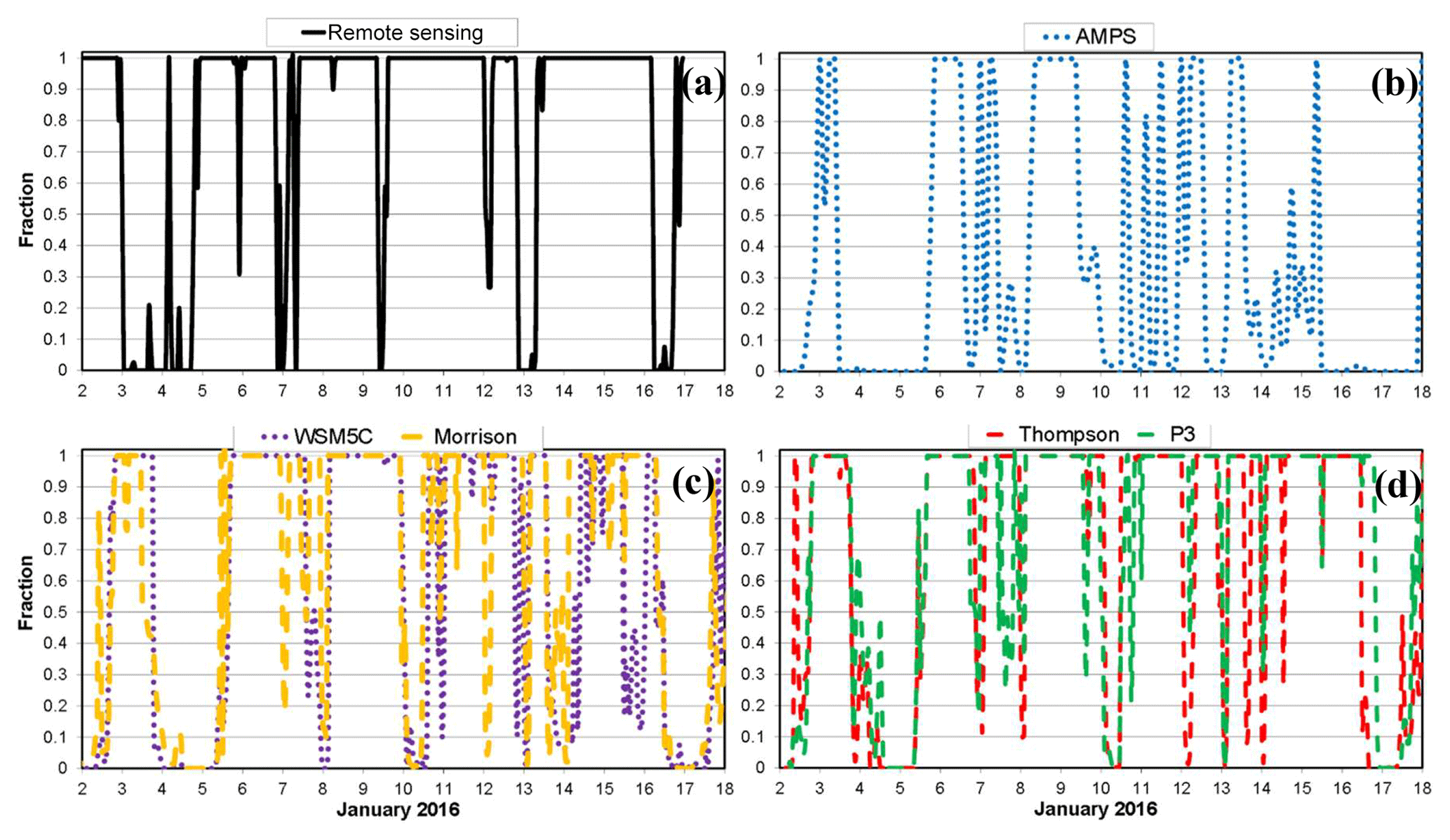
Figure 10Time series of cloud fraction for (a) remote-sensing observations, (b) AMPS, (c) the WSM5C and Morrison simulations, and (d) the Thompson and P3 simulations. Model values of cloud fraction are based upon the Fogt and Bromwich (2008) algorithm using liquid water path and ice water path.
Figure 10 shows times series of cloud occurrence fraction at the WAIS Divide during the MWR availability period. Figure 10a shows values determined from the MPL observations. For the model, however, cloud fraction requires a definition. One earlier method was widely used and defined clouds diagnostically. The cloud fraction was determined based upon factors such as relative humidity, statistic stability, and vertical velocity (Slingo, 1987). With prognostic cloud schemes, cloud fraction is not necessarily a simple function of the condensate, and thus we must consider what value is used for the comparison with observations. One formula that has been used for comparison between model and observations is the cloud fraction formulation of Fogt and Bromwich (2008) calibrated to manual McMurdo Station cloud fraction observations:
where the total cloud fraction is based upon the LWP and IWP in g m−2. The cloud fraction is limited to the maximum value of 1. Cloud occurrence fraction from the MPL is not identical to standard observer-based cloud fraction observations (e.g., Wagner and Kleiss, 2016). However, the instantaneous model cloud fraction by Eq. (2) is typically 1 or very close to 0, and thus the effective differences between cloud fraction and cloud fraction occurrence is minimized for comparisons between model and observations. Equation (2) is especially useful for time-averaged cloud fraction, although the liquid and ice water paths must be instantaneous values, not time-averaged values.
The observed cloud occurrence fraction is frequently 1, and the average is 0.77 during this time (Fig. 10a). Cloud-free times are more common for the AMPS, and thus the average is 0.32 (Fig. 10b). The Polar WRF 3.9.1 simulations show some similarity in their time series of cloud fraction, with the average varying from 0.59 for WSM6C to 0.71 for P3. Microphysics schemes with stronger cloud radiative forcing have larger average total cloud fraction (Figs. 7 and 10).
Liquid cloud occurrence fraction is shown in Fig. 11. Only the first term on the right-hand side of Eq. (2) is used to define modeled liquid cloud fraction. Liquid clouds are frequently observed but are rarely simulated by the AMPS (Fig. 11a). The Morrison scheme simulates liquid clouds much more frequently than WSM5C but not as frequently as the observations. The Thompson and P3 schemes simulate liquid clouds more frequently than the Morrison scheme. Average liquid cloud fractions are 0.65, 0.01, 0.05, 0.20, 0.26, and 0.34 for the observations, AMPS. WSM5C, Morrison, Thompson, and P3, respectively.

Figure 11Time series of liquid cloud fraction for (a) remote-sensing observations and the AMPS, (b) the WSM5C and Morrison simulations, and (c) the Thompson and P3 simulations. Model values of cloud fraction are based upon the Fogt and Bromwich (2008) algorithm.
Figure 12 shows the vertical distribution of cloud fraction. While the observed cloud fraction is again determined by surface-based MPL observations, Eq. (2) is inappropriate for point values of cloud fraction in a column. We select the mixing ratio 0.001 g kg−1 as the classic WRF minimum hydrometer threshold for cloud in the simulations. Model fraction is either 0 or 1 for total condensate concentrations below or above the threshold. The upper troposphere is not shown as the MPL attenuates through cloud layers.

Figure 12Time–height plots of total cloud fraction (color scale) for (a) remote-sensing observations, (b) AMPS, (c) WSM5C, (d) Morrison, (e) Thompson, and (f) P3. Model values of cloud fraction are based upon a condensate mixing ratio threshold of 10−6.
Remote sensing at the WAIS Divide detects clouds that are frequently present below 650 hPa (Fig. 12a). Detectable clouds can decrease with height due to attenuation of the lidar pulse at lower altitudes. Thus, it is not surprising that simulated clouds are appear deeper (Fig. 12b–f). Furthermore, the minimum threshold of 0.001 g kg−1 allows model clouds with the density of very thin cirrus that may be difficult to observe. We found that simulated cloud tops (not shown) are sensitive to the specification of the threshold.
Figure 13 shows liquid cloud occurrence fraction to be more confined to the lower troposphere than total cloud occurrence fraction (Fig. 12). The simulated liquid clouds, when present, are near the surface for the simulations with the WSM5C microphysics (Fig. 13b, c). The more recent microphysics schemes simulate deeper liquid clouds.
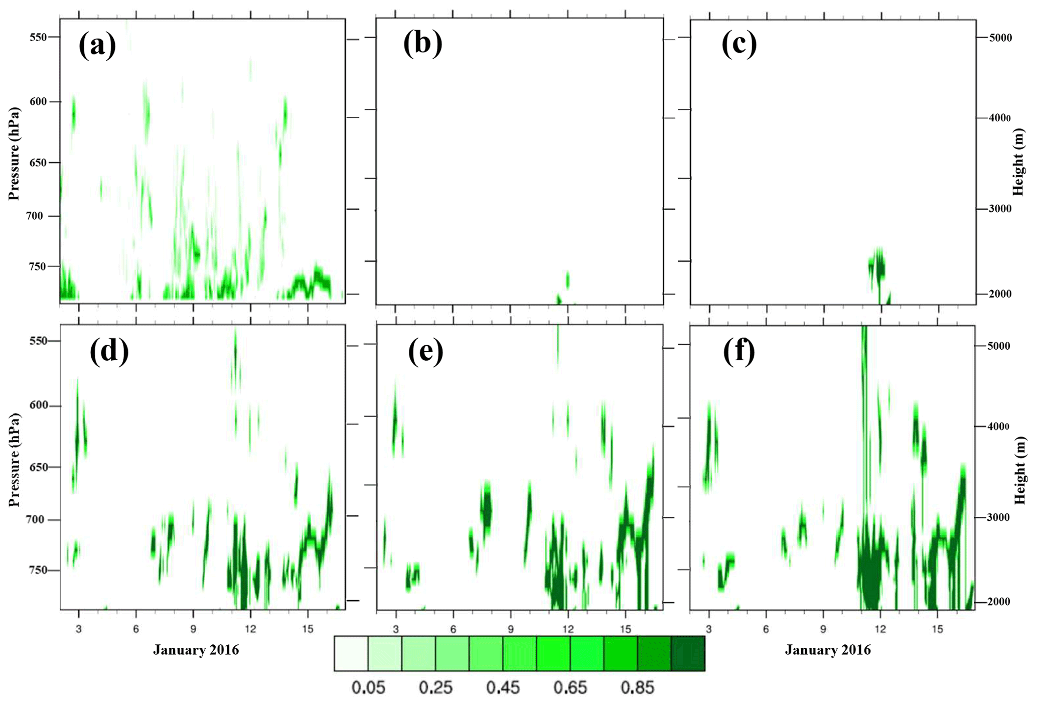
Figure 13Time–height plots of liquid cloud fraction (color scale) for (a) remote-sensing observations, (b) AMPS, (c) WSM5C, (d) Morrison, (e) Thompson, and (f) P3. Model values of cloud fraction are based upon a condensate mixing ratio threshold of 10−6.
Figure 14 shows the mean cloud fraction profiles above sea level (a.s.l.) for the period 2–16 January. As noted earlier, the MPL pulse attenuation likely results in some underestimation of both the total cloud and liquid occurrence fractions at higher elevations. Returning to Fig. 12 that shows shallow clouds with variable vertical structure observed by the MPL, while the simulations have deep, vertically aligned clouds, the means shown in Fig. 14 display this difference in vertical structure. The averaging of frequent deep cloud structures results in high mean values for the simulations, compared to the means of the more variable observations. Therefore, a vertically aligned cloud overlap better represents the simulated clouds than a random overlap. These stacked clouds reduce the modeled cloud fraction shown in Fig. 10, as the middle cloud layer is on of top of the low cloud layer, rather than additive to the cloud fraction. The observed average total cloud fraction peaks at 0.51 at 1985 m a.s.l. (Fig. 14a). The fraction decreases to 0.30 near 2300 m a.s.l. then decreases to 0.10 above 3300 m. The profiles suggest that there could be slightly elevated (liquid-bearing) cloud occurrence at 3935 m a.s.l. The observed liquid cloud fraction is more surface based with a peak of 0.28 at both 1915 and 1985 m a.s.l., and values decreasing to 0.06 at 2210 m (Fig. 14a).

Figure 14Vertical profiles of average cloud fraction over the period 2–16 January 2016 for (a) remote-sensing observations of total cloud fraction and liquid cloud fraction, and (b) observations and simulations of total cloud fraction.
The simulated cloud fraction profile peaks near the surface for the AMPS and WSM5C (Fig. 14b). For the AMPS (WSM5C), the maximum is 0.50 (0.64) at 8 m (84 m) above the surface. The cloud fraction is higher for the recent microphysics schemes, with all having maxima above 0.64 at heights below 2400 m a.s.l. The largest cloud fraction is 0.69 at 2165 m for Thompson.
The mean simulated liquid and ice cloud fractions are shown in Fig. 15. The values are from 2 to 16 January 2016, the same period used for the profiles in Fig. 5. Similar to the profile displayed in Fig. 14, the observations show a more shallow peak in the lower troposphere than in the simulations. (Fig. 15a). The fractions are based upon the total liquid or ice content. P3 has a unique liquid profile that peaks at 0.26 at 2376 m a.s.l.. The Morrison and Thompson simulations have similar liquid cloud fraction profiles with double peaks between 2160 and 2500 m. Figure 15b shows that ice is frequently present in the lowest 1000 m above the surface for the simulations. All the simulations show maxima for ice in the lowest 500 m above the surface, varying from 0.50 at 8 m for the AMPS and 0.49 for P3 at 365 m to 0.64 for 85 m with WSM5C. The Polar WRF 3.9.1 simulations produce more ice cloud fractions than the AMPS.
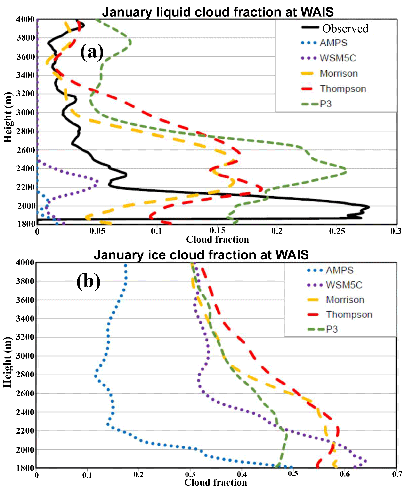
Figure 15Vertical profiles of average cloud fraction over 2–16 January 2016 for (a) liquid cloud fraction and (b) ice cloud fraction.
A sensitivity test referred to as P3-50, was based upon P3 to see if the setting of 400 cm−3 for the liquid droplet number concentration had an important impact on results of that simulation. We set the liquid concentration at 50 cm−3 in the sensitivity test, same as in the simulation with the Morrison microphysics. We use from 12:00 UTC on 6 January to 11:00 UTC on 17 January 2016 as the active period for test results. P3-50 exhibited a reduction of the average LWP from 21 to 16 g m−2, compared to the parent simulation P3. The ice water path is less impacted and reduced by less than 7 %. Figure 16 shows the 2 m temperature and surface downwelling shortwave and longwave radiation. The change in specified liquid concentration has small impact on the 2 m temperature, with the largest impact after 10 January when more noticeable amounts of liquid water were simulated (Figs. 9b and 16a). The average temperature in P3-50 (−9.6 ∘C) is the same as in P3 over the test period. The downwelling shortwave radiation, however, is modified with the local noon on 11, 14, and 15 January showing insolation increases of 50–170 W m−2 (Fig. 16c). P3-50 is an improvement on these days. The impact on the downwelling longwave radiation is much smaller (Fig. 16b). Overall, P3-50 has a net increase (decrease) of 23.9 (2.6) W m−2 in downwelling shortwave (longwave) radiation compared to P3. Since most of the shortwave radiation is reflected off the Antarctic surface, the net impact on the near-surface temperature is small (Fig. 16a).

Figure 16Times series of (a) 2 m temperature (∘C), (b) downwelling longwave radiation (W m−2), and (c) downwelling shortwave radiation (W m−2) during the period 6–17 January 2016 for the observations, the P3 simulation, and P3-50 sensitivity test.
The recent 2015–2017 AWARE field program provides a highly detailed set of remote-sensing and surface observations that can be used to study the simulation Antarctic clouds and the surface energy budget. We focus on the December 2015–January 2016 test period when observations were taken at the WAIS Divide. These observations are used for comparison with the AMPS forecasting system and new simulations with Polar WRF 3.9.1. The AMPS uses the WRF single-moment 5-class microphysics, while the new Polar WRF 3.9.1 simulations are run with WSM5C and three more recent microphysics schemes. These are the Morrison 2-moment microphysics, the Thompson–Eidhammer aerosol-aware microphysics, and the new Morrison–Milbrandt P3 microphysics.
The AMPS simulates few liquid hydrometers during austral summer at the WAIS Divide, even though liquid clouds are frequently observed by the MPL, primarily a consequence of the WSM5C microphysics in the AMPS. Consequently, downwelling shortwave radiation is excessive at the surface, while downwelling longwave radiation is too small. The WSM5C simulation with Polar WRF 3.9.1 has reduced biases of the same sign. The decreased magnitude in WSM5C appears due to GFS forcing of initial and boundary conditions for the AMPS while ERA-I is used for WSM5C. Simulated hydrometers are overwhelmingly composed of ice with WSM5C.
The more advanced microphysics schemes show considerable improvement in the simulation of overall cloud fraction, liquid hydrometers, and cloud radiative effects. The instantaneous simulation of liquid remains somewhat problematic even given the improvements. The Morrison scheme simulates less LWP and weaker cloud radiative forcing than the Thompson and P3 schemes. P3 simulates the greatest LWP and cloud radiative effect. All schemes appear to underestimate total cloud fraction and liquid cloud fraction at the WAIS Divide. The vertical distribution of simulated cloud properties differs from observed profiles, with deeper clouds simulated than observed, although the MPL may not detect the upper regions of clouds due to attenuation.
In the near future, the more extensive AWARE cloud observations at McMurdo Station over the full seasonal cycle will provide a basis for sensitivity tests designed to seek Antarctic optimizations to the advanced microphysics schemes used for the WAIS Divide. In particular, we plan to work with two more advanced implementations of the P3 microphysics (Milbrandt and Morrison, 2016). Sensitivity tests will also vary the background IN concentrations in simulations with the Thompson microphysics, as the limited observational evidence suggests that the contributing aerosol concentrations may vary or are unknown over a range of orders of magnitude.
The standard release of WRF can be downloaded from NCAR Mesoscale and Microscale Meteorology (2019). The polar optimizations can be requested from Polar Meteorology Group (2019).
All the observations from the AWARE field campaign (including the reprocessed MPL dataset) can be downloaded from the ARM Data Discovery website (https://www.archive.arm.gov/discovery/, last access: 27 September 2019). AMPS forecast fields in original WRF format are available from NCAR (2019). Selected AMPS output fields for March 2006–December 2016 for grids 2–6 can be downloaded from Polar Meteorology Group (2017).
KMH was the primary author and coordinated with the other authors. KMH conducted the Polar WRF simulations, downloaded and processed AWARE data, and processed the model data.
DHB coordinated the Ohio State component of AWARE and was the primary co-author. DHB read and provided input on all drafts of the manuscript and helped plan the simulations.
SHW processed the AMPS data for the manuscript.
IS processed the MPL and cloud mask data. IS provided advice on the use of these data.
JV coordinated the Penn State component of AWARE. JV provided advice on Antarctic clouds and the AWARE data.
DL was the overall coordinator of AWARE. DL provided advice on Antarctic clouds and the AWARE project and helped to coordinate the use of CERES data.
The authors declare that they have no conflict of interest.
Any opinions presented here are those of the paper authors alone and are not necessarily those of Atmospheric Chemistry and Physics.
Numerical simulations were performed on the Intel Xeon cluster at the Ohio Supercomputer Center, which is supported by the state of Ohio. We thank Julien Nicolas for providing rawinsonde, surface energy balance and LWP observations for the WAIS Divide and thank Ryan Scott for providing cloud forcing derived from CERES. All the observations from the AWARE field campaign (including the reprocessed MPL dataset) can be downloaded from the ARM Data Discovery website (http://www.archive.arm.gov/discovery/, last access: 9 August 2019). This is Contribution 1584 of the Byrd Polar and Climate Research Center.
This research has been supported by the U.S. Department of Energy, Office of Science (DOE (grant no. DE-SC0017981)) and National Science Foundation (NSF (grant no. PLR 1443443)).
This paper was edited by Timothy J. Dunkerton and reviewed by two anonymous referees.
Andreas, E. L, Horst, T. W., Grachev, A. A., Persson, P. O. G., Fairall, C. W., Guest, P. S., and Jordan, R. E.: Parametrizing turbulent exchange over summer sea ice and the marginal ice zone, Q. J. Roy. Meteor. Soc., 136, 927–943, https://doi.org/10.1002/qj.618, 2010.
Barker, D. M., Huang, W., Guo, Y.-R., Bourgeois, A. J., and Xiao, Q.-N.: A three-dimensional (3DVAR) data assimilation system for use with MM5: Implementation and initial results, Mon. Weather Rev., 132, 897–914, https://doi.org/10.1175/1520-0493(2004)132<0897:ATVDAS>2.0.CO;2, 2004.
Barlage, M., Chen, F., Tewari, M., Ikeda, K., Gochis, D., Dudhia, J., Rasmussen, R., Livneh, B., Ek, M., and Mitchell, K.: Noah land model modifications to improve snowpack prediction in the Colorado Rocky Mountains, J. Geophys. Res., 115, D22101, https://doi.org/10.1029/2009JD013470, 2010.
Bracegirdle, T. J. and Marshal, G. J.: The reliability of Antarctic tropospheric pressure and temperature in the latest global reanalyses, J. Climate, 25, 7138–7146, https://doi.org/10.1175/JCLI-D-11-00685.1, 2012.
Bromwich, D. H., Hines, K. M., and Bai, L. S.: Development and testing of Polar WRF: 2. Arctic Ocean, J. Geophys. Res., 114, D08122, https://doi.org/10.1029/2008JD010300, 2009.
Bromwich, D. H., Nicolas, J. P., Hines, K. M., Kay, J. E., Key, E., Lazzara, M. A., Lubin, D., McFarquhar, G. M., Gorodetskaya, I., Grosvenor, D. P., Lachlan-Cope, T. A., and van Lipzig, N.: Tropospheric clouds in Antarctica, Rev. Geophys., 50, RG1004, https://doi.org/10.1029/2011RG000363, 2012.
Bromwich, D. H., Nicolas, J. P., Monaghan, A. J., Lazzara, M. A., Keller, L. M., Weidner, G. A., and Wilson, A. B.: Central West Antarctica among the most rapidly warming regions on Earth, Nat. Geosci., 6, 139–145, https://doi.org/10.1038/ngeo1671, 2013a.
Bromwich, D. H., Otieno, F. O., Hines, K., Manning, K., and Shilo, E.: Comprehensive evaluation of polar weather research and forecasting performance in the Antarctic, J. Geophys. Res., 118, 274–292, https://doi.org/10.1029/2012JD018139, 2013b.
Bromwich, D. H., Nicolas, J. P., Monaghan, A. J., Lazzara, M. A., Keller, L. M., Weidner, G. A., and Wilson, A. B.: Corrigendum: Central West Antarctica among the most rapidly warming regions on Earth, Nat. Geosci., 7, 76, https://doi.org/10.1038/ngeo2016, 2014.
Cadeddu, M.: G-Band Vapor Radiometer Profiler (GVRP) Handbook, Office of Science, DOE Office of Biological and Environmental Research, USA, DOE/SC-ARM/TR-091, https://doi.org/10.2172/982364, 2010.
Cadeddu, M. P., Turner, D. D., and Liljegren, J. C.: A Neural Network for Real-Time Retrievals of PWV and LWP From Arctic Millimeter-Wave Ground-Based Observations, IEEE T. Geosci. Remote, 47, 1887–1900, https://doi.org/10.1109/TGRS.2009.2013205, 2009.
Cassano, J. J., DuViviera, A., Roberts, A., Hughes, M., Seefeldt, M., Brunke, M., Craig, A., Fisel, B., Gutowski, W., Hamman, J., Higgins, M., Maslowski, W., Nijssen, B., Osinski, R., and Zeng, X.: Development of the Regional Arctic System Model (RASM): Near surface atmospheric climate sensitivity, J. Climate, 30, 5729–5753, https://doi.org/10.1175/JCLI-D-15-0775.1, 2017.
Chou, M. D., Suarez, M. J., Liang, X. Z., and Yan, M. M. H.: A thermal infrared radiation parameterization for atmospheric studies, NASA/TM-2001-104606, 19, 56 pp., 2001.
Clough, S. A., Shephard, M. W., Mlawer, E. J., Delamere, J. S., Iacono, M. J., Cady-Pereira, K., Boukabara, S., and Brown, P. D.: Atmospheric radiative transfer modeling: A summary of the AER codes, J. Quant. Spectrosc. Ra., 91, 233–244, https://doi.org/10.1016/j.jqsrt.2004.05.058, 2005.
Cook, D.: ARM: Surface Energy Balance System (SEBS) Handbook, Atmospheric Radiation Measurement (ARM) Archive, Oak Ridge National Laboratory, Argonne, IL, 2018.
Cooper, W. A.: Ice initiation in natural clouds, Precipitation Enhancement – A Scientific Challenge, Meteorol. Mon., 29–32, 1986.
Deb, P., Orr, A., Hosking, J. S., Phillips, T., Turner, J., Bannister, D., Pope, J. O., and Colwell, S.: An assessment of the Polar Weather Research and Forecasting (WRF) model representation of near-surface meteorological variables over West Antarctica, J. Geophys. Res., 121, 1532–1548, https://doi.org/10.1002/2015jd024037, 2016.
DeConto, R.M., Pollard, D.: Contributions of Antarctica to past and future sea level rise, Nature, 531, 591–597, https://doi.org/10.1038/nature17145, 2016.
Dee, D.P., Uppala, S.M., Simmons, A.J., Berrisford, P., Poli, P., Kobayashi, S., Andrae, U., Balmaseda, M.A., Balsamo, G., Bauer, P., Bechtold, P., Beljaars, A.C.M., van de Berg, L., Bidlot, J., Bormann, N., Delsol, C., Dragani, R., Fuentes, M., Geer, A.J., Haimberger, L., Healy, S.B., Hersbach, H., Holm, E.V., Isaksen, L.,i Kalberg, P., Kohler, M., Matricardi, M., McNally, A.P., Monge-Sanz, B.M., Morcrette, J.-J., Park, B.-K., Peubey, C., de Rosnay, P., Tavolato, C., Thepaut, J.-N., Vitart, F.: The ERA-Interim reanalysis: Configuration and performance of the data assimilation system, Q. J. Roy. Meteor. Soc., 137, 553–597, https://doi.org/10.1002/qj.828, 2011.
Dooraghi, M., Reda, I., Xie, Y., Morris, V., Andreas, A., Kutchenreiter, M., Habte, A., and Sengupta, M.: ARM: Sky Radiation Sensor: 60-Second Downwelling Irradiances (Atmospheric Radiation Measurement (ARM) Archive, Oak Ridge National Laboratory (ORNL), https://doi.org/10.5439/1025281, 1996.
Flynn, C. J., Mendoza, A., Zheng, Y., and Mathurb, S.: Novel polarization-sensitive micropulse lidar measurement technique, Opt. Express, 15, 2785–2790, https://doi.org/10.1364/OE.15.002785, 2007.
Fogt, R. L. and Bromwich, D. H.: Atmospheric moisture and cloud cover characteristics forecast by AMPS, Weather Forecast., 23, 914–930, https://doi.org/10.1175/2008/WAF2006100.1, 2008.
Grosvenor, D. P., Choularton, T. W., Lachlan-Cope, T., Gallagher, M. W., Crosier, J., Bower, K. N., Ladkin, R. S., and Dorsey, J. R.: In-situ aircraft observations of ice concentrations within clouds over the Antarctic Peninsula and Larsen Ice Shelf, Atmos. Chem. Phys., 12, 11275–11294, https://doi.org/10.5194/acp-12-11275-2012, 2012.
Hines, K. M. and Bromwich, D. H.: Development and testing of Polar Weather Research and Forecasting (WRF) model. Part I: Greenland Ice Sheet meteorology, Mon. Weather Rev., 136, 1971–1989, https://doi.org/10.1175/2007MWR2112.1, 2008.
Hines, K. M. and Bromwich, D. H.: Simulation of late summer Arctic clouds during ASCOS with Polar WRF, Mon. Weather Rev., 145, 521–541, https://doi.org/10.1175/MWR-D-16-0079.1, 2017.
Hines, K. M., Bromwich, D. H., Bai, L.-S., Barlage, M., and Slater, A. S.: Development and testing of polar Weather Research and Forecasting Model: Part III. Arctic land, J. Climate, 24, 26–48, https://doi.org/10.1175/2010JCLI3460.1, 2011.
Hines, K. M., Bromwich, D. H., Bai, L., Bitz, C. M., Powers, J. G., and Manning, K. W.: Sea ice enhancements to Polar WRF, Mon. Weather Rev., 143, 2363–2385, https://doi.org/10.1175/MWR-D-14-00344.1, 2015.
Hogan, A. W.: Aerosol exchange in the remote troposphere, Tellus, 38, 197–213, 1986.
Holdridge, D. and Kyrouac, J.: ARM: ARM-Standard Meteorological Instrumentation at Surface (Atmospheric Radiation Measurement (ARM) Archive, Oak Ridge National Laboratory (ORNL), https://doi.org/10.5439/1025220, 1993.
Hong, S.-Y., Dudhia, J., and Chen, S.-H.: A revised approach to ice microphysical processes for the bulk parameterization of clouds and precipitation, Mon. Weather Rev., 132, 103–120, https://doi.org/10.1175/1520-0493(2004)132<0103:ARATIM>2.0.CO;2, 2004.
Janjć, Z. I.: The step-mountain Eta coordinate model: Further developments of the convection, viscous sublayer, and turbulence closure schemes, Mon. Weather Rev., 122, 927–945, https://doi.org/10.1175/1520-0493(1994)122<0927:TSMECM>2.0.CO;2, 1994.
Kain, J. S.: The Kain–Fritsch convective parameterization: An update, J. Appl. Meteorol., 43, 170–181, https://doi.org/10.1175/1520-0450(2004)04360;0170:tkcpau62;2.0.co;2, 2004.
Kato, S., Rose F. G., Sun-Mack S., Miller W. F., Chen Y., Rutan D. A., Stephens G. L., Loeb N. G., Minnis P., Wielicki B. A., Winker D. M., Charlock T. P., Stackhouse P. W., Xu K.-M., and Collins W.: Computation of top-of-atmosphere and surface irradiances with CALIPSO, CloudSat, and MODIS-derived cloud and aerosol properties. J. Geophys. Res., 116, D19209. https://doi.org/10.1029/2011JD016050, 2011.
King J. C., Gadian, A., Kirchgaessner, A., Kuipers, Munneke, P., Lachlan-Cope, T. A., Orr, A., Reijmer, C., van den Broeke, M. R., van Wessem, J. M., and Weeks, M.: Validation of the summertime surface energy budget of Larsen C Ice Shelf (Antarctica) as represented in three high-resolution atmospheric models, J. Geophys. Res., 120, 1335–1347, https://doi.org/10.1002/2014JD022604, 2015.
Klein, S. A., McCoy, R. B., Morrison, H., Ackerman, A. S., Avramov, A., de Boer, G. Chen, M., Cole, J. N. S., Del Genio, A., Falk, M., Foster, M. J., Fridlind, A. M., Golaz, J.-C., Hashino, T., Harrington, J. Y., Hoose, C., Khairoutdinov, M., Larson, V. E., Liu, X., Luo, Y., McFarquhar, G., Menon, S., Neggers, R. A. J., Park, S., Poellot, M., Schmidt, J. M., Sednev, I., Shipway, B. J., Shupe, M. D., Spangenberg, D., Sud, Y. C., Turner, D. D., Veron, D. E., von Salzen, K., Walker, G., Wang, Z., Wolf, A.B., Xie, S., Xu, K., Yang, F., and Zhang G.: Intercomparison of model simulations of mixed-phase clouds observed during the ARM Mixed-Phase Arctic Cloud Experiment. Part I: Single-layer cloud, Q. J. Roy. Meteor. Soc., 135, 979–1002, https://doi.org/10.1002/qj.416, 2009.
Lachlan-Cope, T., Listowski, C., and O'Shea, S.: The microphysics of clouds over the Antarctic Peninsula – Part 1: Observations, Atmos. Chem. Phys., 16, 15605–15617, https://doi.org/10.5194/acp-16-15605-2016, 2016.
Lazzara, M. A., Weidner, G. A., Keller, L. M., Thom, J. E., and Cassano, J. J.: Antarctic Automatic Weather Station Program: 30 years of polar observations, B. Am. Meteorol. Soc., 93, 1519–1537, https://doi.org/10.1175/BAMS-D-11-00015.1, 2012.
Listowski, C. and Lachlan-Cope, T.: The microphysics of clouds over the Antarctic Peninsula – Part 2: modelling aspects within Polar WRF, Atmos. Chem. Phys., 17, 10195–10221, https://doi.org/10.5194/acp-17-10195-2017, 2017.
Lubin, D., Chen, B., Bromwich, D. H., Somerville, R. C. J., Lee, W.-H., and Hines, K. M.: The impact of Antarctic cloud radiative properties on a GCM climate simulation, J. Climate, 11, 447–462, https://doi.org/10.1175/1520-0442(1998)0112.0, 1998.
Mather, J. H. and Voyles, J. W.: The ARM climate research facility: A review of structure and capabilities, B. Am. Meteorol. Soc., 94, 377–392, https://doi.org/10.1175/BAMS-D-11-00218.1, 2013.
McCoy, D. T., Hartmann, D. L., Zelinka, M. D., Ceppi, P., and Grosvenor, D. P.: Mixed-phase cloud physics and Southern Ocean cloud feedback in climate models, J. Geophys. Res., 120, 9539–9554, https://doi.org/10.1002/2015JD023603, 2015.
Milbrandt, J. A. and Morrison, H.: Parameterization of cloud microphysics based on the prediction of bulk ice particle properties. Part III: Introduction of multiple free categories, J. Atmos. Sci., 73, 975–995, https://doi.org/10.1175/JAS-D-15-0204.1, 2016.
Milbrandt, J. A. and Yau, M. K.: A multimoment bulk microphysics parameterization. Part II: A proposed three-moment closure and scheme description, J. Atmos. Sci., 62, 3065–3081, https://doi.org/10.1175/JAS3535.1, 2005.
Morris, V. R.: Microwave radiometer (MWR) handbook, ARM-TR-016, DOE Office of Science, Office of Biological and Environmental Research, 20 pp., https://doi.org/10.2172/1020715, 2006.
Morrison, H. and Milbrandt, J. A.: Parameterization of cloud microphysics based on the prediction of bulk ice particle properties. Part I: Scheme description and idealized tests, J. Atmos. Sci., 72, 287–311, https://doi.org/10.1175/JAS-D-14-0065.1, 2015.
Morrison, H. and Pinto, J. O.: Intercomparison of bulk cloud microphysics schemes in mesoscale simulations of springtime Arctic mixed-phase stratiform clouds, Mon. Weather Rev., 134, 1880–1990, 2006.
Morrison, H., Curry, J. A., and Khvorostyanov, V. I.: A new double-moment microphysics scheme for application in cloud and climate models. Part I: Description, J. Atmos. Sci., 62, 1665–1677, https://doi.org/10.1175/JAS3446.1, 2005.
Morrison, H., Pinto, J. O., Curry, J. A., and McFarquhar, G. M.: Sensitivity of modeled Arctic mixed-phase stratocumulus to cloud condensation and ice nuclei over regionally varying surface conditions, J. Geophys. Res., 113, D05203, https://doi.org/10.1029/2007JD008729, 2008.
Morrison, H., Thompson, G., and Tatarskii, V.: Impact of cloud microphysics on the development of trailing stratiform precipitation in a simulated squall line: Comparison of one- and two-moment schemes, Mon. Weather Rev., 137, 991–1007, https://doi.org/10.1175/2008MWR2556.1, 2009.
Nakanishi, M. and Niino, H.: An improved Mellor-Yamada level-3 model: Its numerical stability and application to a regional prediction of advection fog, Bound.-Lay. Meteorol., 119, 397–407, https://doi.org/10.1007/s10546-005-9030-8, 2006.
NCAR Mesoscale and Microscale Meteorology: The Weather Research and Forecasting model, available at: https://www.mmm.ucar.edu/weather-research-and-forecasting-model, last accessed 7 August 2019.
Nicolas, J. P. and Bromwich, D. H.: Climate of West Antarctica and influence of marine air intrusions, J. Climate, 24, 49–67, https://doi.org/10.1175/2010JCLI3322.1, 2011.
Nicolas, J. P. and Bromwich, D. H.: New reconstruction of Antarctic near-surface temperatures: Multidecadal trends and reliability of global reanalyses, J. Climate, 27, 8070–8093, https://doi.org/10.1175/JCLI-D-13-00733.1, 2014.
Nicolas, J. P, Scott, R. C., Cadeddu, M. P., Bromwich, D. H., Verlinde, J., Lubin, D., Russell, L. M., Jenkinson, C., Powers, H. H., Ryczek, M., Stone, G., and Wille, J.: January 2016 extensive summer melt in West Antarctica favoured by strong El Nino, Nat. Commun., 8, 15799, https://doi.org/10.1038/ncomms15799, 2017.
NOAA Environmental Modeling Center: The GFS Atmospheric Model, NCEP Office Note 442, 14 pp., available at: https://www.emc.ncep.noaa.gov/officenotes/newernotes/on442.pdf (last access: 27 September 2019), 2003.
O'Shea, S. J., Choularton, T. W., Flynn, M., Bower, K. N., Gallagher, M., Crosier, J., Williams, P., Crawford, I., Fleming, Z. L., Listowski, C., Kirchgaessner, A., Ladkin, R. S., and Lachlan-Cope, T.: In situ measurements of cloud microphysics and aerosol over coastal Antarctica during the MAC campaign, Atmos. Chem. Phys., 17, 13049–13070, https://doi.org/10.5194/acp-17-13049-2017, 2017.
Pavolonis, M. and Key, J.: Antarctic cloud radiative forcing at the surface estimated from the AVHRR Polar Pathfinder and ISCCP D1 datasets, 1985–93, J. Appl. Meteorol., 42, 827–840, https://doi.org/10.1175/1520-0450(2003)042<0827:ACRFAT>2.0.CO;2, 2003.
Polar Meteorology Group: AMPS database, available at: http://polarmet.osu.edu/AMPS/, last access: 29 September 2017.
Polar Meteorology Group: The Polar WRF model, available at: http://polarmet.osu.edu/PWRF/registration.php, last access: 7 August 2019.
Pon, K.: The representation of low cloud in the Antarctic Mesoscale Prediction System, MS thesis, Atmospheric Sciences Program, Dept. of Geography, The Ohio State University, 80 pp., 2015.
Powers, J. G., Manning, K. W., Bromwich, D. H., Cassano, J. J., and Cayette, A. M.: A decade of Antarctic science support through AMPS, B. Am. Meteorol. Soc., 93, 1699–1712, https://doi.org/10.1175/BAMS-D-11-00186.1, 2012.
Rignot, E.: Changes in West Antarctic ice stream dynamics observed with ALOS PALSAR data, Geophys. Res. Lett., 35, L12505, https://doi.org/10.1029/2008GL033365, 2008.
Schmeisser, L., Backman, J., Ogren, J. A., Andrews, E., Asmi, E., Starkweather, S., Uttal, T., Fiebig, M., Sharma, S., Eleftheriadis, K., Vratolis, S., Bergin, M., Tunved, P., and Jefferson, A.: Seasonality of aerosol optical properties in the Arctic, Atmos. Chem. Phys., 18, 11599–11622, https://doi.org/10.5194/acp-18-11599-2018, 2018.
Scott, R. C. and Lubin, D.: Unique manifestations of mixed-phase cloud microphysics over Ross Island and the Ross Ice Shelf, Antarctica, Geophys. Res. Lett., 43, 2936–2945, https://doi.org/10.1002/2013JD021132, 2016.
Scott, R. C., Lubin, D., Vogelmann, A. M., and Kato, S.: West Antarctic Ice Sheet cloud cover and surface radiation budget from NASA A-Train satellites, J. Climate, 30, 6151–6170, https://doi.org/10.1175/JCLI-D-16-0644.1, 2017.
Shupe, M. and Intrieri, J.: Cloud radiative forcing of the Arctic surface: The influence of cloud properties, surface albedo, and solar zenith angle, J. Climate, 17, 616–628, https://doi.org/10.1175/1520-0442(2004)017<0616:CRFOTA>2.0.CO;2, 2004.
Shupe, M. D.: Clouds at Arctic atmospheric observatories. Part II: Thermodynamic phase characteristics, J. Appl. Meteorol. Clim., 50, 645–661, https://doi.org/10.1175/2010JAMC2468.1, 2011.
Silber, I., Verlinde, J., Eloranta, E. W., and Cadeddu, M.: Antarctic cloud macrophysical, thermodynamic phase, and atmospheric inversion coupling properties at McMurdo Station: I. Principal data processing and climatology, J. Geophys. Res., 123, 6099–6121, https://doi.org/10.1029/2018JD028279, 2018a.
Silber, I., Verlinde, J., Eloranta, E. W., Flynn, C. J., and Flynn, D. M.: Reprocessed MPL data sets, https://doi.org/10.5439/1468777, 2018b.
Silber, I., Verlinde, J., Eloranta, E. W., Flynn, C. J., and Flynn, D. M.: Polar liquid cloud base detection algorithms for high spectral resolution or micropulse lidar data, J. Geophys. Res.-Atmos., 123, 4310–4322, https://doi.org/10.1029/2017JD027840, 2018c.
Skamarock, W. C., Klemp, J. B., Dudhia, J., Gill, D. O., Barker, D. M., Duda, M. G., Huang, X.-Y., Wang, W., and Powers, J. G: A description of the Advanced Research WRF Version 3, NCAR Tech, Note NCAR/TN-475+STR, 125 pp., 2008.
Slingo, J. M.: The development and verification of a cloud prediction scheme for the ECMWF model, Q. J. Roy. Meteor. Soc., 113, 899–927, https://doi.org/10.1002/qj.49711347710, 1987.
Solomon, A., Shupe, M. D., Persson, P. O. G., and Morrison, H.: Moisture and dynamical interactions maintaining decoupled Arctic mixed-phase stratocumulus in the presence of a humidity inversion, Atmos. Chem. Phys., 11, 10127–10148, https://doi.org/10.5194/acp-11-10127-2011, 2011.
Solomon, A., Shupe, M. D., Persson, O., Morrison, H., Yamaguchi, T., Caldwell, P. M., and de Boer, G.: The sensitivity of springtime Arctic mixed-phase stratocumulus clouds to surface-layer and cloud-top inversion-layer moisture sources, J. Atmos. Sci., 71, 574–595, https://doi.org/10.1175/JAS-D-13-0179, 2014.
Solomon, A., Feingold, G., and Shupe, M. D.: The role of ice nuclei recycling in the maintenance of cloud ice in Arctic mixed-phase stratocumulus, Atmos. Chem. Phys., 15, 10631–10643, https://doi.org/10.5194/acp-15-10631-2015, 2015.
Steig, E. J. Schneider, D. P., Rutherford, S. D., Mann, M. E., Comiso, J. C., and Shindell, D. T.: Warming of the Antarctic ice-sheet surface since the 1957 International Geophysical Year, Nature, 457, 459–462, https://doi.org/10.1038/nature07669, 2009.
Thompson, G., and Eidhammer, T.: A study of aerosol impacts on clouds and precipitation development in a large winter cyclone, J. Atmos. Sci., 71, 3636–3658, https://doi.org/10.1175/JAS-D-13-0305.1, 2014.
Thompson, G., Field, P. R., Rasmussen, R. M., and Hall, W. D.: Explicit forecasts of winter precipitation using an improved bulk microphysics scheme. Part II: Implementation of a new snow parameterization, Mon. Weather Rev., 136, 5095–5115, https://doi.org/10.1175/2008MWR2387.1, 2008.
Tjernström, M., Leck, C., Birch, C. E., Bottenheim, J. W., Brooks, B. J., Brooks, I. M., Bäcklin, L., Chang, R. Y.-W., de Leeuw, G., Di Liberto, L., de la Rosa, S., Granath, E., Graus, M., Hansel, A., Heintzenberg, J., Held, A., Hind, A., Johnston, P., Knulst, J., Martin, M., Matrai, P. A., Mauritsen, T., Müller, M., Norris, S. J., Orellana, M. V., Orsini, D. A., Paatero, J., Persson, P. O. G., Gao, Q., Rauschenberg, C., Ristovski, Z., Sedlar, J., Shupe, M. D., Sierau, B., Sirevaag, A., Sjogren, S., Stetzer, O., Swietlicki, E., Szczodrak, M., Vaattovaara, P., Wahlberg, N., Westberg, M., and Wheeler, C. R.: The Arctic Summer Cloud Ocean Study (ASCOS): overview and experimental design, Atmos. Chem. Phys., 14, 2823–2869, https://doi.org/10.5194/acp-14-2823-2014, 2014.
Turner, J., Lachlan-Cope, T. A., Colwell, S., Marshall, G. J., and Connolley, W. M.: Significant warming of the Antarctic winter troposphere, Science, 311, 1914–1917, https://doi.org/10.1126/science.1121652, 2006.
van Tricht K., Lhermitte, S., Lenaerts, J. T. M., Gorodetskaya, I. V., L'Ecuyer, T. S., Noah, B., van den Broeke, R., Turner D. D., and van Lipzig, N. P. M.: Clouds enhance Greenland ice sheet meltwater runoff, Nat. Commun., 7, 10266, https://doi.org/10.1038/ncomms10266, 2016.
Wagenbach, D., Gorlach, U., Moser, K., and Munnich, K. O.: Coastal Antarctic aerosol: the seasonal pattern of its chemical composition and radionuclide content, Tellus B, 40, 426–436, 1988.
Wagner, T. J. and Kleiss, J. M.; Error characteristics of ceilometer-based observations of cloud amount, J. Atmos. Ocean. Tech., 33, 1557–1567, https://doi.org/10.1175/JTECH-D-15-0258.1, 2016.
Wille, J. D., Bromwich, D. H., Cassano, J. J., Nigro, M. A., Mateling, M. E., and Lazzara, M. A.: Evaluation of the AMPS boundary layer simulations on the Ross Ice Shelf, Antarctica, with unmanned aircraft observations, J. Appl. Meteorol. Clim., 56, 2239–2258, https://doi.org/10.1175/JAMC-D-16-0339.1, 2017.
Wilson, A. B., Bromwich, D. H., and Hines, K. M.: Evaluation of Polar WRF forecasts on the Arctic System Reanalysis domain: Surface and upper air analysis, J. Geophys. Res., 116, D11112, https://doi.org/10.1029/2010JD015013, 2011.
Wilson, A. B., Bromwich, D. H., and Hines, K. M.: Evaluation of Polar WRF forecasts on the Arctic System Reanalysis domain. Part II. Atmospheric hydrologic cycle, J. Geophys. Res., 117, D04107, https://doi.org/10.1029/2011JD016765, 2012.
Witze, A.: Antarctic clouds studied for first time in five decades, Nature, 529, 12–12, https://doi.org/10.1038/529012a, 2016.