the Creative Commons Attribution 4.0 License.
the Creative Commons Attribution 4.0 License.
 | 07 Oct 2019
Wintertime aerosol measurements during the Chilean Coastal Orographic Precipitation Experiment
Sara Lynn Fults
Adam K. Massmann
Aldo Montecinos
Elisabeth Andrews
David E. Kingsmill
Justin R. Minder
René D. Garreaud
The Chilean Coastal Orographic Precipitation Experiment (CCOPE) was a 3-month field campaign (June, July and August 2015) that investigated wintertime coastal rain events. Reported here are analyses of aerosol measurements made at a coastal site during CCOPE. The aerosol monitoring site was located near Arauco, Chile. Aerosol number concentrations and aerosol size distributions were acquired with a condensation particle counter (CPC) and an ultra high sensitivity aerosol spectrometer (UHSAS). Arauco CPC data were compared to values measured at the NOAA observatory Trinidad Head (THD) on the northern Pacific coast of California. The winter-averaged CPC concentration at Arauco is 2971 ± 1802 cm−3; at THD the average is 1059 ± 855 cm−3. Despite the typically more pristine South Pacific region, the Arauco average is larger than at THD (p<0.01). Aerosol size distributions acquired during episodes of onshore flow were analyzed with Köhler theory and used to parameterize cloud condensation nuclei activation spectra. In addition, sea salt aerosol (SSA) concentration was parameterized as a function of sea surface wind speed. It is anticipated these parameterizations will be applied in modeling of wintertime Chilean coastal precipitation.
- Article
(3014 KB) -
Supplement
(1451 KB) - BibTeX
- EndNote


Forecast error due to incomplete understanding of atmospheric aerosols is evident in the predictions of many atmospheric models. As an example, general circulation models (GCMs) are used to forecast the Earth system's response to emissions of both aerosols and greenhouse gases. In spite of several decades of GCM development, the effect of aerosols on the future climate remains uncertain (Boucher et al., 2013), particularly when compared to the greater certainty in climate forcing from anthropogenic greenhouse gases (e.g., Hansen, 2009, his Fig. 10).
Aerosols perturb the abundance of cloud droplets and rain drops within clouds warmer than 0 ∘C (liquid-only clouds). Consequently, upward reflection of solar radiation by liquid-only clouds (Twomey, 1974), and upward reflection attributable to cloud fractional coverage (Albrecht, 1989), increase with increased aerosol abundance. Commonly referred to as aerosol indirect effects on climate, these processes decrease the amount of solar energy absorbed by the Earth system and thus oppose global warming due to greenhouse gases. Other aerosol indirect effects, for example those due to aerosols nucleating ice in mixed-phase clouds (McCoy et al., 2014), augment greenhouse gas warming.
Because of its lower population and lower intensity of anthropogenic aerosol emissions, the Southern Hemisphere has been explored as a region for conducting studies of aerosol indirect effects and for exploring contrasts with the Northern Hemisphere (Schwartz, 1988). This study contributes to previous investigations of Southern Hemispheric aerosols during winter (Gras, 1990, 1995; Yum and Hudson, 2004). We emphasize the following topics: (1) the parameterized relationship between sea salt aerosol (SSA) particles (diameter >0.5 µm) and wind speed, (2) cloud condensation nuclei (CCN), i.e., particles that are both smaller and more numerous than the above-mentioned SSA, (3) the parameterized relationship describing CCN activation spectra (Rogers and Yau, 1989; chap. 6), and (4) the potential application of the SSA and CCN parameterizations in numerical modeling of wintertime Southern Hemispheric clouds and precipitation. Motivating our investigation are modeling studies (Feingold et al., 1999), and analyses of field measurements (Gerber and Frick, 2012), indicating that the reduction of rainfall due to increased CCN can be negated by SSA particles.
Measurements made with a condensation particle counter (CPC), an instrument that reports the concentration of particles with a diameter (D) larger than ∼0.01 µm, have formed the basis of many previous investigations of aerosol abundance (Gras, 1990; Brechtel et al., 1998; Dall'Osto et al., 2010; Andreae, 2009). These studies also evaluated air parcel back trajectories and demonstrated that marine source regions are characterized by distinctly smaller concentrations than continental regions. Measurements of aerosol size distributions (ASDs) can also aid understanding of the contrast between marine and continental conditions (Brechtel et al., 1998; Birmili et al., 2001; Raes et al., 1997). The latter studies investigated accumulation mode particles, centered at ∼0.1 µm, and particles sizing in a mode at a distinctly smaller central diameter (∼0.05 µm). This smaller mode is commonly referred to as the Aitken mode. In marine settings, the coexistence of both modes has been attributed to in-cloud conversion of gas-phase sulfur dioxide (SO2) to aerosol-phase sulfate (Hoppel et al., 1994), to coalescence scavenging occurring within clouds (Hudson et al., 2015), and to new particle formation (Covert et al., 1992; Petters et al., 2006). The latter process occurs in environments with sufficiently enhanced ratios of SO2 relative to aerosol.
The present work is an analysis of CPC and ASD measurements acquired at a coastal site on the central Chilean Pacific coast during the Southern Hemisphere winter (June, July, and August). Aerosol measurements were made during the Chilean Coastal Orographic Precipitation Experiment (CCOPE) in 2015. CCOPE investigated aerosol properties and coastal orographic precipitation and meteorology (Massmann et al., 2017).
This paper is organized into the following sections. Section 2 has descriptions of the aerosol and meteorological instruments used to make surface measurements during CCOPE, and Sect. 3 describes our analysis methods. Section 4 includes four topics: (1) analysis of CPC measurements and comparison to coastal North Pacific measurements, (2) development of a relationship between size-integrated aerosol concentration and size-integrated aerosol volume and comparison to similar relationships derived for summertime stratocumulus regimes, (3) development of a parameterization of CCN activation spectra, and (4) development of a parameterization of SSA number concentration. In Sect. 5, we compare our findings to previous work, and in Sect. 6 we conclude with an outlook for how our parameterizations could be applied in modeling of wintertime central Chilean Pacific coast clouds and precipitation.
2.1 Measurement site
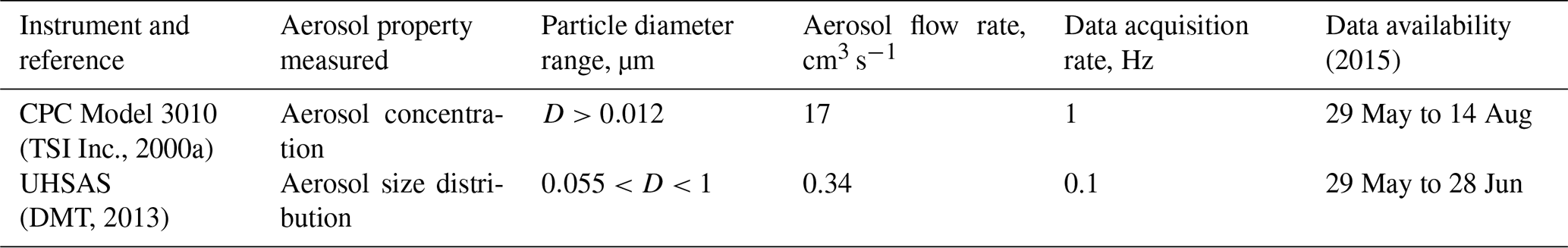
During CCOPE, a CPC (model 3010; TSI Inc., 2000a) and an ultra high sensitivity aerosol spectrometer (UHSAS) (DMT, 2013) were operated at a residence (37.25∘ S, 73.34∘ W, 55 m above mean sea level, m.s.l.) near Arauco, Chile (population 35 000). Arauco is a coastal town on the central Chilean Pacific coast. Our measurement site, hereafter the Arauco site (Fig. 1), was selected because of our aim to characterize aerosols advecting onto South America from the southeastern Pacific. Related to this, our measurements were coordinated with investigations of rainfall inside the domain portrayed in Fig. 1. This study region lies in the South Pacific winter storm track, and rainfall here can be strongly enhanced by the Nahuelbuta Range (Garreaud et al., 2016; Massmann et al., 2017). During CCOPE, several rainfall events were studied using profiling radars and a precipitation disdrometer deployed at Curanilahue (Fig. 1), as well as a network of precipitation gauges. The Arauco site is located on a forested hill; most of the population of Arauco lives east of the Arauco site at an elevation less than 20 m m.s.l.

Figure 1Central Chilean coastal region and the location of the Arauco site, where aerosol measurements were made during CCOPE. Altitude thresholds for the digital elevation map are at 0, 50, 250, 500, 750, and 1000 m m.s.l.
Salient characteristics of the CPC and UHSAS are provided in Table 1. These instruments were operated inside the residence at the Arauco site. In addition, a 3 m meteorological tower was deployed adjacent to the residence. Thermodynamic state (i.e., T, P, and humidity) and horizontal wind speed and direction were measured on the tower. CPC and meteorological measurements (minus wind direction) were acquired from 29 May to 14 August (Table 1), UHSAS measurements were acquired from 29 May to 28 June (Table 1), and wind direction measurements were acquired from 19 June to 14 August.
2.2 Instrumentation
Here we discuss characteristics of the CPC and UHSAS, sampling of the ambient CCOPE aerosol, data acquisition of CPC and UHSAS measurements during CCOPE, and use of the recorded UHSAS histograms to calculate ASDs. Additional information about the UHSAS is provided in Appendix A. In that appendix we discuss how we validated, in a laboratory, the UHSAS's determination of test aerosol concentration and particle size. During those validation studies we intentionally dried the test aerosols to a relative humidity (RH) ≤15 %. Consequently, the effect of aerosol-bound water on either the physical size or the refractive index of the test particles was negligible. UHSAS sizing of partially dried haze droplets (RH ≤ 60 %), sampled from the ambient atmosphere during CCOPE, and an associated particle size overestimate, is also discussed in Appendix A. In Appendix A, we estimate the particle size overestimate to be ∼20 %.
During CCOPE, the CPC and UHSAS sampled ambient aerosol through a section of copper tube (length = 3 m; inner diameter = 0.003 m; volumetric flow rate = 34 cm3 s−1). The inlet end of the tube (hereafter, the sample tube) was secured below an eave on the west side of the residence at the Arauco site. The Reynolds number (Re) of the flow within the sample tube was 960 and thus well below the value (Re=2300) where laminar flow changes to turbulent flow. Particle transmission efficiencies were evaluated using Eq. (7.29) in Hinds (1999). These are 78 % for D=0.01 µm particles and ≥99 % for D=0.1 µm and D=1 µm particles.
The CPC counts particles larger than D=0.012 µm (Table 1) 1 up to a maximum concentration of 10 000 cm−3. CPC data were recorded once per second (Table 1). The UHSAS measures scattering produced when aerosol particles are drawn through light emitted by a solid-state laser (λ=1.05 µm). By reference to a calibration table (Cai et al., 2008, 2013), the UHSAS microprocessor converts scattered light intensity to particle size and accumulates the derived sizes in a 99-channel histogram. Channel widths are logarithmically uniform (Δlog 10D=0.013) over the instrument's full range ( µm).
Equation (1) was used to calculate the ASD.
Here Δni is the “ith” component of the count histogram and is the aerosol flow rate. During CCOPE, the UHSAS aerosol flow rate and the particle count histogram were recorded once every 10 s (Table 1), and hence the sample interval (Δt in Eq. 1) is 10 s.
3.1 Air mass classification and air parcel trajectories
Locations close to the Arauco site are shown in Fig. 1. A significant pollution source in the region is the Arauco paper mill, which releases 600 t yr−1 of SO2 (Arauco Woodpulp, 2010). When winds had an easterly component, the paper mill may have affected air quality at the Arauco site. Other pollution sources are Concepción (population 950 000), Coronel (population 110 000), Curanilahue (population 32 000), Lebu (population 24 000), and Cañete (population 32 000). In addition, many residences in the region, including the residence where we operated the CPC and UHSAS, burn wood for residential heating.
In a subsequent section, we compare CPC data from the Arauco site to values measured at NOAA's Trinidad Head (THD) observatory in northern California (41.05∘ N, 124.2∘ W, 107 m m.s.l.). The THD dataset includes contamination from local sources (e.g., campfires lit by day visitors at the Trinidad State Beach Picnic Ground). Additionally, McKinleyville, CA (population 15 000), and Arcata, CA (population 18 000), are the two coastal population centers reasonably close to THD. Both are southeast of THD, at distances between 15 and 25 km. Northern California's large population centers (the San Francisco Bay Area and Sacramento) are ∼300 km southeast of THD. An important distinction between the sampling at THD and Arauco is the above ground level (a.g.l.) height of the aerosol inlets. This is 10 and 2 m a.g.l. at THD and Arauco, respectively. We cannot state with any certainty if the lower-height sampling at Arauco made those measurements unrepresentative.
Wind measurements made at the Arauco site (Sect. 2.1) and THD were used to conditionally sample the CPC measurements. At Arauco, wind directions from 180 to 330∘ were chosen as the clean sector. At THD, the clean sector was chosen from 210 to 360∘. The clean sectors at Arauco and THD are shown in Fig. 2. Three factors contributed to our selection of the clean sectors: (1) inclusion of winds from either true south (Arauco site) or true north (THD), (2) the same range of angles (150∘) at both sites, and (3) exclusion of wind from the directions of regional population centers.
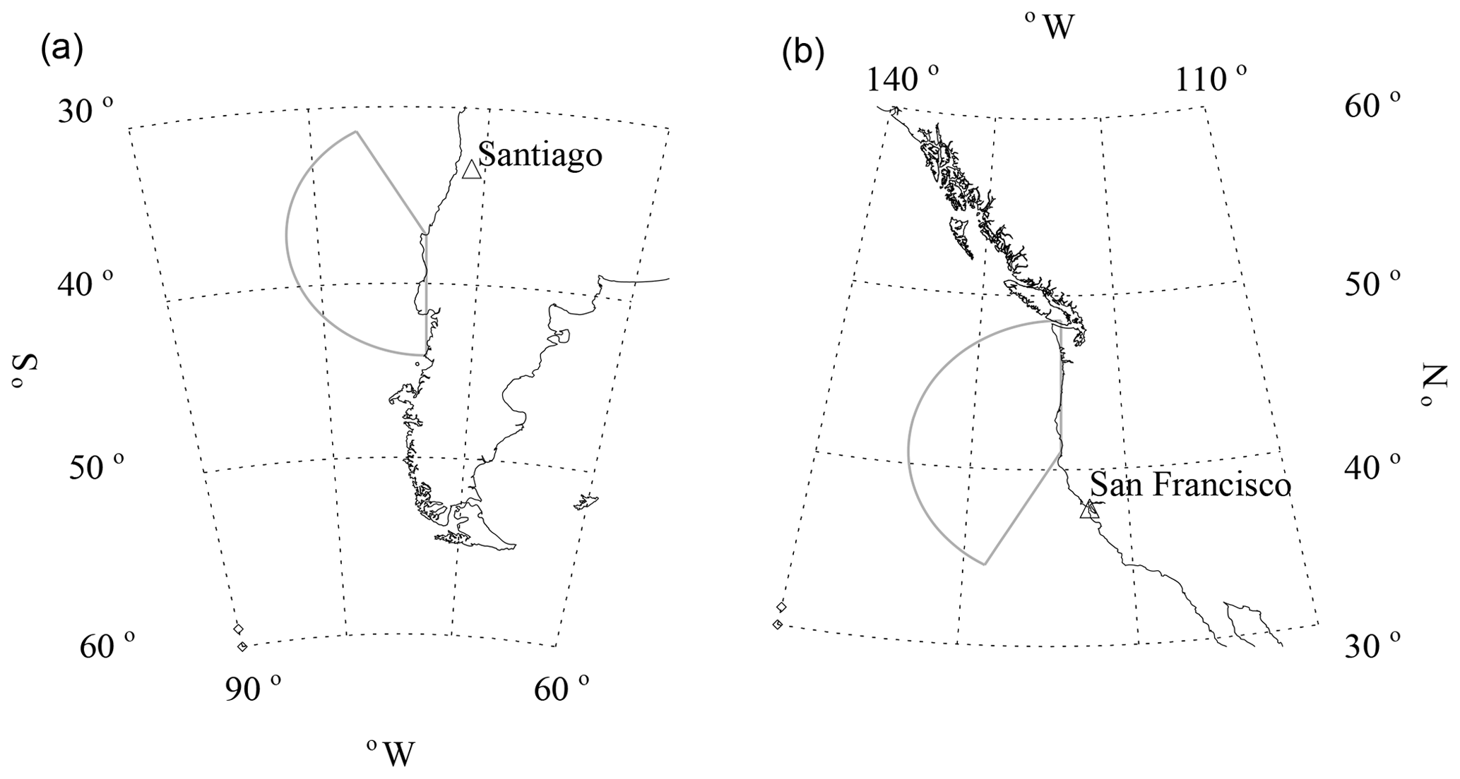
Figure 2Clean sector chosen for Arauco (a, 180 to 330∘) and the clean sector chosen for THD (b, 210 to 360∘).
Additionally, we used HYSPLIT back trajectories (NOAA, 2016) to conditionally sample Arauco site aerosol measurements associated with onshore-moving air. The back trajectories were initialized at 00:00, 06:00, 12:00, and 18:00 UTC. In addition to these static arrival times, trajectories were calculated with the coordinates of the Arauco site2 and with wind fields from the Global Data Assimilation System. The spatial resolution of the wind data is 0.5∘. Position along a trajectory was evaluated hourly. Trajectories that were over the ocean continuously for 3 d before landfall, and had a direction within the clean sector 1 h before arriving at Arauco, were classified as “onshore” trajectories. There are 20 onshore trajectories that overlap with the availability of CCOPE UHSAS measurements.
In subsequent sections, a set of twenty 2 h data segments, centered on the onshore trajectory arrival times, are further analyzed. Appendix B describes the numerical filter we used to derive the aerosol properties analyzed in Sect. 4.2, 4.3, 4.4, and 4.5. The filter attenuates aerosol property variability occurring on timescales shorter than 100 s. We developed the filter to remove narrow “spikes” in the concentration sequences (CPC and UHSAS), which seem to have originated from local sources of aerosol pollution. The Supplement has plots of filtered aerosol properties corresponding to each of the twenty 2 h segments. Four of these were impacted aerosol variability at scales larger than 100 s. In general, these features were not attenuated by the numerical filter. In these instances we discarded (subjectively) portions of the 2 h segment and retained a subset for the analyses conducted in Sect. 4.3, 4.4 and 4.5.
Trajectory altitude is important for determining the presence of SSA particles. Onshore trajectories originating from relatively close to the sea surface, and thus classified as onshore “sea surface” trajectories, were required to have pressures >980 hPa over their 3 d advection to the Arauco site. A total of 18 of the 20 onshore trajectories were also sea surface trajectories. An example of a sea surface trajectory is shown in Fig. 3a–b. The sea surface wind speed (U), analyzed in Sect. 4.5, is the average of the 6-hourly trajectory speeds in the 6 h window ending 6 h before the trajectory arrived at the Arauco site. The averaging interval is shown in Fig. 3b. Two onshore trajectories, classified as “aloft”, had pressures substantially smaller than 980 hPa over their 3 d advection to the Arauco site.

Figure 3(a) One of the 18 sea surface trajectories that arrived at the Arauco site between 29 May to 28 June; this trajectory arrival occurred at 00:00 UTC 9 June. Black dots are hourly output of the HYSPLIT model; however, for clarity, only every other 1 h point is plotted. (b) Hourly parcel mean sea level (MSL) altitude vs. time; however, for clarity, only every other 1 h point is plotted. The averaged sea surface wind speed (U) was evaluated over the 12:00 to 18:00 UTC interval shown in gray. The MSL altitude was calculated using the pressure output by HYSPLIT (parcel barometric pressure) and the ICAO equation for the Standard Atmosphere (ICAO, 1993). The MSL altitude increases if a larger sea-level is pressure applied in the ICAO equation. This sensitivity is ∼8 m hPa−1.
3.2 Sea salt aerosol
Correlated values of SSA concentration and sea surface wind speed are reported in many publications. In a review of the topic, Lewis and Schwartz (2004; hereafter LS04) used a particle's deliquesced wet size, evaluated at 80 % relative humidity, to group SSA particles into three size classes. In field studies conducted at a coastal site, Clarke et al. (2003) demonstrated that particles sizing in the middle of LS04's small particle size class – those with a dry diameter larger than 0.5 µm or a RH = 80 % wet diameter larger than 1 µm – had a composition that was dominated by sea salt (NaCl).
By restricting our focus to segments of the CCOPE data associated with sea surface trajectories (Sect. 3.1), we will analyze UHSAS measurements of particles with D>0.5 µm (N>0.5) and will assume that this subset of the ASD corresponds to SSA particles. This lower-limit size is a factor of 2 smaller than the RH = 80 % diameter corresponding to the middle of LS04's small SSA class. This is because we assumed that particle size decreased as the aerosol stream warmed from its ambient temperature to the temperature of the UHSAS measurement. Support for this assumption is provided in Appendix A.
3.3 Moments of the aerosol size distribution
In our analysis, we calculated three moments of the UHSAS-measured ASDs. These are the aerosol concentration (NUHSAS), aerosol surface area (SUHSAS), and aerosol volume (VUHSAS). We symbolize these moments as integrals (Eqs. 2–4).
In these formulae the group represents the concentration of aerosol particles with a diameter between log 10D and log 10D+dlog 10D. Hence, when plotted versus the logarithm of particle diameter, the area under the dN∕dlog 10D curve is proportional to the size-integrated concentration. This is demonstrated in Fig. 4a–b, where the size-integrated concentration is ∼300 cm−3 in onshore-moving air (Fig. 4a), and the concentration is approximately 4 times larger (∼1100 cm−3) in air thought to be contaminated by continental sources (Fig. 4b). Also apparent is the right tail of an Aitken mode, at ∼0.06 µm in Fig. 4a (onshore-moving air), the absence of an Aitken mode in Fig. 4b (continental air), at least at diameters detectable by the UHSAS (D>0.055 µm; Table 1), and the presence of an accumulation mode at ∼0.1 µm in both air masses (Fig. 4a–b). Two aspects of these results, i.e., the absence of an Aitken mode plus the dominance of an accumulation mode in polluted coastal air is consistent with ASDs reported in Raes et al. (1997) and in Dall'Osto et al. (2010).
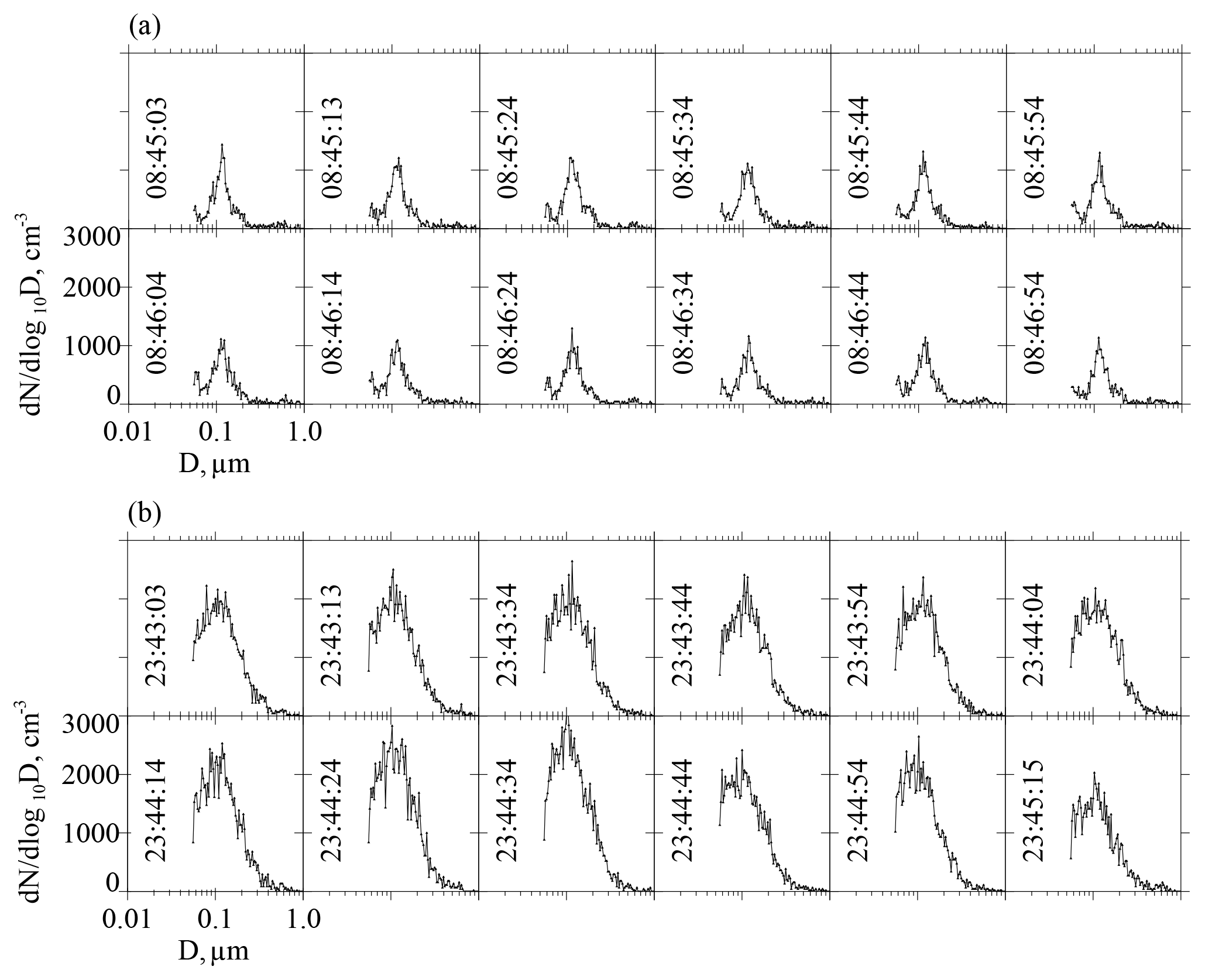
Figure 4Consecutive ASDs recorded by the UHSAS at the Arauco site. (a) ASDs with a relatively small concentration (∼300 cm−3), a right tail of an Aitken mode (at ∼0.06 µm), and an accumulation mode (at ∼0.1 µm), in onshore-moving air on 5 June 2015. (b) ASDs with a proportionately larger concentration (∼1100 cm−3), an accumulation mode (at ∼0.1 µm), and no evidence of an Aitken mode, in air thought to be contaminated by continental sources (4 June 2015). Time is written in UTC in each panel.
4.1 Comparison of CPC data from the Arauco site and THD
In this section, CPC-measured concentrations from the Arauco site and from NOAA's THD observatory are compared. At THD, CPC measurements were made using a TSI 3760 condensation particle counter. The minimum particle diameter detected by the TSI 3760 (D=0.015 µm; Wiedensohler et al., 1997) is slightly larger than that in the TSI 3010 (D=0.012 µm; Table 1). We ignored this distinction.
The THD dataset spans the years 2002 to 2014. Because CCOPE was a wintertime field study, only December, January, and February THD data are used in the comparison. There are 24 346 data points (hourly averaged) from THD and 5541 classify as clean sector. In comparison, there are 745 data points from the Arauco site (hourly averaged) and 194 classify as clean sector. For both sites, we required a clean sector wind speed >1.5 m s−1 in addition to the clean sector directional criteria (Fig. 2). Because the numerical filter (Sect. 3.1) requires 1 Hz CPC measurements and since 1 Hz measurements are unavailable in the THD data archive, the filter was not applied to either of the data sets analyzed in this section.
Table 2Classification of air mass type.
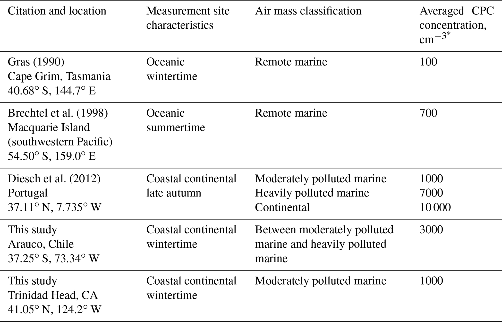
* Values rounded to one significant digit.
In the following paragraph we compare hourly averaged CPC-measured concentrations from the Arauco site and THD. Because the number of data points in these data sets is different, a particular statistical comparison methodology was applied. The approach followed here compares the Arauco and THD average concentrations by applying the Student's t distribution method (t test), explained in Havlicek and Crain (1988; their Eqs. 10.6 and 10.7). The statistical hypotheses are (A) null hypothesis, averages are equal, and (B) alternate hypothesis, averages are different. We also applied the nonparametric Wilcoxon rank-sum test (rs_test; Interactive Data Language, Harris Geospatial Solutions, Inc.). Statistical inferences that we derive based on the Wilcoxon rank-sum test (not shown) are consistent with what we describe below using the t test.
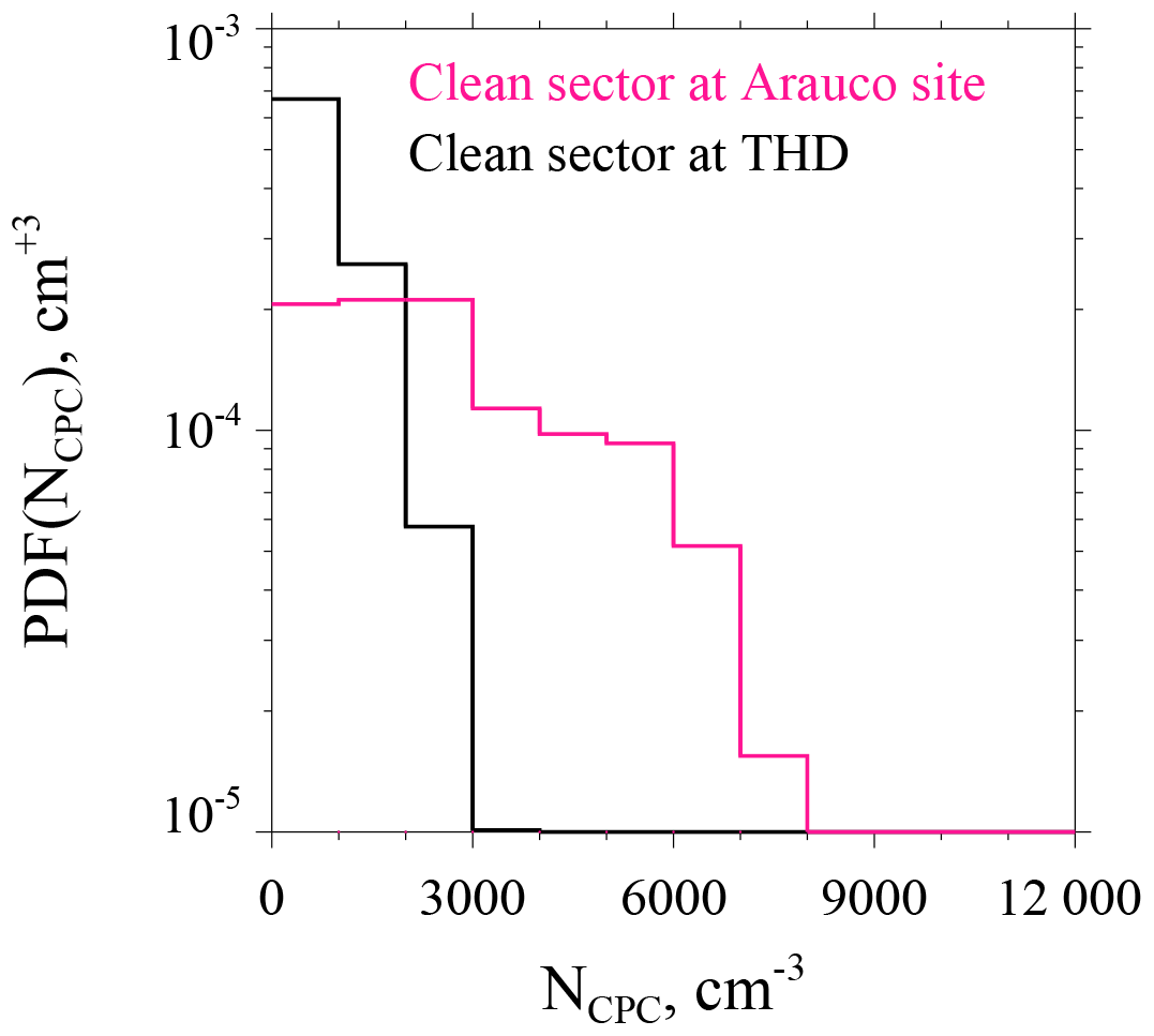
Two aspects of the Arauco–THD comparison are presented here; more detail is available in Fults (2016). First, clean sector measurements are compared. The mean NCPC at Arauco is 2759 cm−3 (standard deviation σ=1827 cm−3). The mean and σ at THD are 858±729 cm−3. Figure 5 shows the Arauco and THD NCPC probability distribution functions. Of note is the larger mode concentration and broader distribution at Arauco. Based on our t test comparison, the Arauco average is larger than the THD average (p<0.01). Second, Arauco and THD concentrations are compared without regard to wind direction. The average at the Arauco site is 2971 ± 1802 cm−3, while at THD the average is 1059 ± 855 cm−3. These averages are also statistically different (p<0.01), and, again, the Arauco average is larger than that at THD. Based on averages presented in this section and information provided in Table 2, two summary statements are warranted: (1) during wintertime, THD is classified as a moderately polluted marine site, and the Arauco site classifies between moderately polluted marine and heavily polluted marine. (2) These sites are not representative of conditions well removed from anthropogenic influence.
4.2 Continental contamination
In this section we probe why aerosol properties varied strongly during 4 of the 20 onshore trajectories. Among these, the example presented in Fig. 6a–c exhibits the largest degree of CPC and UHSAS variability. During this 2 h data segment, centered on 00:00 UTC 9 June (21:00 local time), winds were light at Arauco and Curanilahue (≤1 m s−1) and the wind direction was variable at Curanilahue (Arauco site wind direction measurements are only available after 19 June 2015; Sect. 2.1).
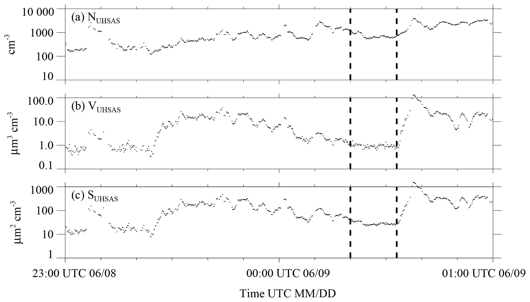
Figure 6Aerosol properties centered on 1 of the 20 onshore trajectories that arrived at the Arauco site between 29 May to 28 June. This trajectory arrival occurred at 00:00 UTC on 9 June. (a) UHSAS concentration; (b) UHSAS aerosol volume; (c) UHSAS aerosol surface area. Aerosol properties shown here were filtered using the procedure described in Appendix B. Vertical dashed lines mark the subset of the 2 h segment we picked (subjectively) as being representative of onshore-moving air that was relatively unaffected by continental aerosols compared to adjacent portions of the 2 h segment.
Over the ocean, 12 to 6 h prior to 00:00 UTC 9 June, the HYSPLIT wind speed was 8.3 m s−1 and the HYSPLIT direction was westerly (Fig. 3a). In terms of UHSAS measurements (Fig. 6a–c), an obvious feature is the variability in the sequences of NUHSAS, VUHSAS, and SUHSAS. The SUHSAS is largest during an enhancement at ∼ 00:37 UTC. The question arises of whether winds over the ocean and the resultant SSA production can cause this variability or if continental aerosol sources have to be evoked to explain this phenomenon. This was addressed by calculating aerosol surface areas as a function of wind speeds that bracket the HYSPLIT-derived wind speed (8.3 m s−1). The basis for this calculation is the S-on-U parameterization described in LS04 (their Fig. 22). The calculation indicates that S can range between 6 µm2 cm−3 (U=6.3 m s−1) and 15 µm2 cm−3 (U=10.3 m s−1). Since the upper-limit of the predicted variation is small compared to SUHSAS at ∼ 00:37 UTC (Fig. 6c) and at other times in Fig. 6c and because the wind speed variation applied in the calculation is an order of magnitude larger than the variation in the HYSPLIT-derived wind speed (±0.1 m s−1), it is concluded that the aerosol enhancements seen in Fig. 6a–c are not due to a wind speed increase over the ocean. Rather, we surmise that aerosols emitted by continental Chilean sources were sampled during portions of the segment in Fig. 6. Vertical dashed lines indicate the subset of the 2 h segment we picked (subjectively) as being representative of onshore-moving air that was not affected, or only moderately affected, by emissions from continental Chilean sources. However, we do not expect our conditional sampling (based on HYSPLIT) and subjective picking (e.g., Fig. 6) to select aerosol properties representative of pristine marine air. Rather, we view these strategies as way to isolate aerosol properties associated with onshore-moving air that was less affected by continental sources compared to the other portions of the CCOPE data set.
Portions of three other 2 h segments were also discriminated into a period of onshore-moving air that was less affected by continental aerosols compared to an adjacent portion (or portions) of the 2 h data segment. This is shown in the Supplement. Only measurements seen plotted between the vertical dashed lines in the Supplement are analyzed in Sect. 4.3, 4.4, and 4.5.
4.3 Using N∕V ratios to parameterize cloud droplet concentration
In this section we analyze two ASD moments (Sect. 3.3). The ratio of NUHSAS (aerosol concentration) and VUHSAS (aerosol volume) – generically the N∕V ratio – is of interest for several reasons. First, for both operational and theoretical reasons the N∕V ratio is evaluated for particle diameters larger than ∼0.1 µm (van Dingenen et al., 2000, hereafter VD00; Hegg and Kaufman, 1998, hereafter HK98), and, importantly, the model developed to evaluate aerosol exchange between an overlying free troposphere (FT) and the marine boundary layer (MBL) successfully predicts the N∕V ratio in the MBL (VD00). Second, a value of the ratio can be derived by fitting measurements of N and V (HK98). Third, aerosol mass loading and thus an aerosol volume corresponding to an assumed particle density3 are relatively easy to evaluate. A method routinely used to evaluate aerosol mass loading involves pulling aerosol-laden air through a filter and evaluating the accumulated mass gravimetrically. Fourth, the product of an N∕V ratio and an ambient aerosol volume (aerosol mass) has been proposed as a scheme for estimating cloud droplet concentration in marine stratocumulus clouds (HK98 and VD00).
HK98 used a passive cavity aerosol spectrometer probe (PCASP) to evaluate N, V, and the N∕V ratio. Since the UHSAS counts down to a smaller diameter (0.055 µm) than the PCASP (0.12 µm), it is expected that the N∕V ratios we derive using the UHSAS will be larger than those in HK98. The main reason for this is that decreasing the lower-limit diameter increases N more than V (VD00).
As in HK98, linear least-squares regression analysis with an equation of the form was used to derive N∕V ratios. Values of NUHSAS and VUHSAS entered into the regressions were derived with the lower-limit diameter set at 0.055 µm (Table 3) and 0.12 µm (Table 4). The latter allows comparison to N∕V ratios in HK98. Tables 3 and 4 show the ratios and the fact that all of the Pearson correlation coefficients (r) are positive. With the exception of trajectories arriving at 12:00 UTC, 5 June, 06:00 UTC, 8 June (Table 3), and 00:00 UTC, 9 June (Table 4), all of the N∕V correlations are statistically significant at p<0.01.
Table 3Statistics for onshore trajectories (particle diameter integration in Eqs. 2, 4, and 5 is from 0.055 to 1 µm).

a DDHHMM indicates the start and end times (day in June 2015, hour, minute) of the data segment. b Pearson product moment for the NUHSAS(D=0.055 µm) on VUHSAS(D=0.055 µm) correlation. c Data recording ended at DDHHMM = 080646, i.e., 14 min before the stated end time.
Table 4Statistics for onshore trajectories (D integration in Eqs. 2, 4, and 5 is from 0.120 to 1 µm).
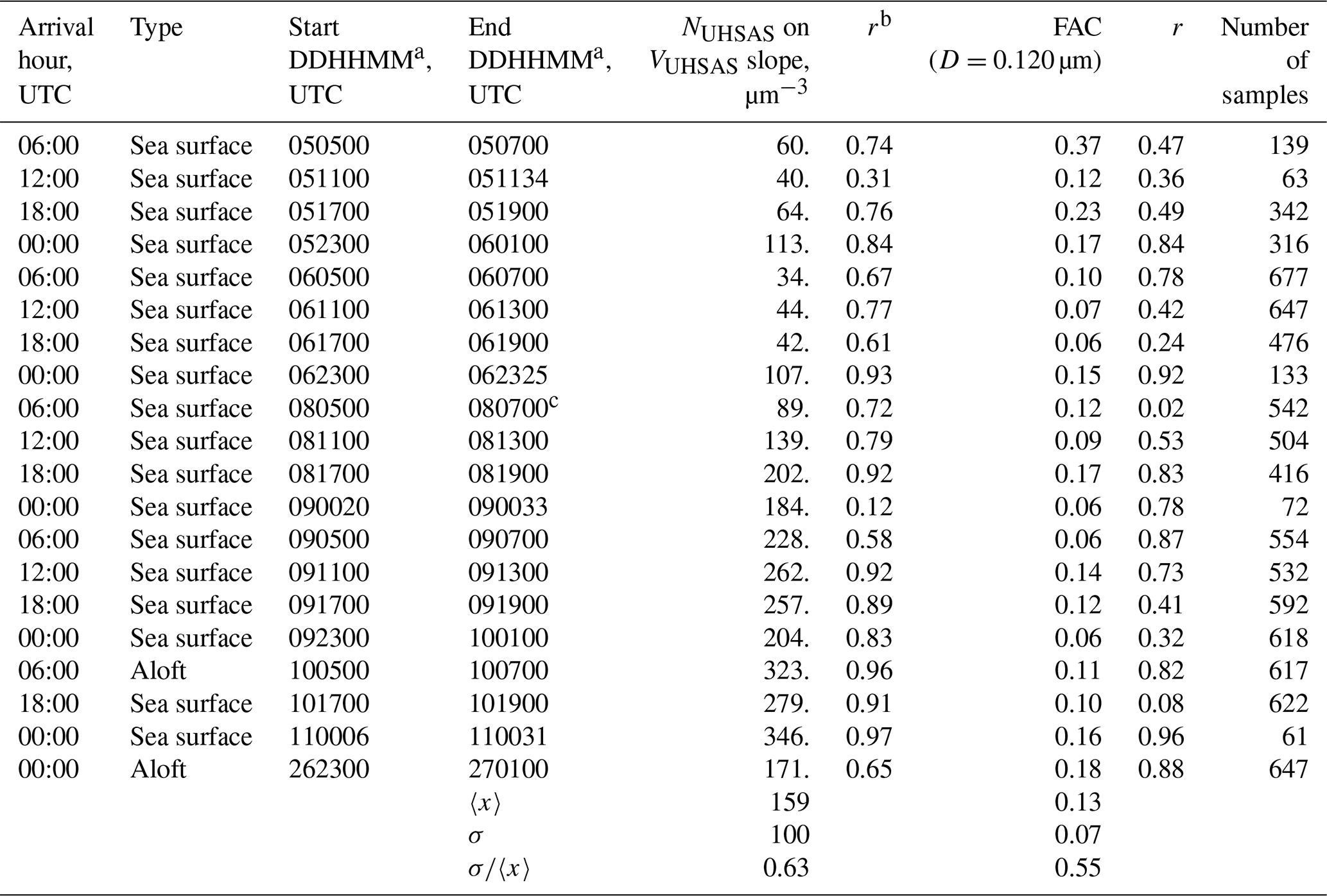
a DDHHMM indicates the start and end times (day in June 2015, hour, minute) of the data segment. b Pearson product moment for the NUHSAS(D=0.120 µm) on VUHSAS(D=0.120 µm) correlation. c Data recording ended at DDHHMM = 080646, i.e., 14 min before the stated end time.
As expected, the average N∕V ratio in the fifth column of Table 3 (417±297 µm−3) is larger than that in HK98 (223±76 µm−3). These averages are different at p=0.01. Table 4 has results based on the larger lower-limit diameter (0.12 µm). In that comparison, the Arauco N∕V ratio (159±100 µm−3) does not differ significantly from HK98's (i.e., p>0.01).
Application of the N∕V ratio to cloud–aerosol–precipitation modeling requires knowledge of the aerosol volume, or alternatively, knowledge of the aerosol mass loading and the aerosol particle density. The aerosol volume is then multiplied by an average N∕V ratio (e.g., the average at the bottom of the fifth column of Table 4), and their product is taken to be the modeled cloud droplet concentration (HK98 and VD00). This is straightforward, at least from the perspective of incorporating an aerosol-induced cloud feedback into a simulation, but it suffers from requiring additional information about the aerosol (aerosol volume). Because the UHSAS was unavailable for much of CCOPE (Table 1), aerosol volume is also unavailable. Another drawback is the implicit assumption that only aerosol particles larger than the lower-limit diameter (e.g., 0.12 µm in Table 4) form cloud droplets.
4.4 Using size distribution and NCPC to parameterize CCN activation spectra
Andreae (2009) analyzed a set of aerosol concentration measurements obtained from colocated CPC and CCN instruments. Andreae's CPC measurements represent the concentration of particles no smaller than a particular diameter (∼0.01 µm; Sect. 2.2), and his CCN measurements represent the concentration of particles that activate cloud droplets at a water vapor supersaturation (SS) no larger than a particular value (Rogers and Yau, 1989; chap. 6). The latter is SS = 0.4 % in Andreae (2009).
Similar to the relationship between CCN concentration at SS = 0.4 % and CPC concentration (Andreae, 2009; his Fig. 2), we now describe how CPC and UHSAS data from CCOPE can be used to develop a function that describes CCN activation spectra. In the parameterization we develop, the independent variable is a CPC-measured aerosol concentration. While only estimates, the activation spectra we obtain represent an important step toward evaluating how CCN affected cloud and precipitation during CCOPE. We envision this assessment will be advanced when our activation spectra are used to initialize numerical models.
Our first step is to select a particle diameter, apply this as a lower-limit diameter in an integration of the UHSAS size distribution, and divide the integral by the coincident CPC-measured concentration. The result is referred to as the fractional aerosol concentration (FAC).
Figure 7a–b have graphical representations of FAC(D=0.055 µm) and FAC(D=0.120 µm).
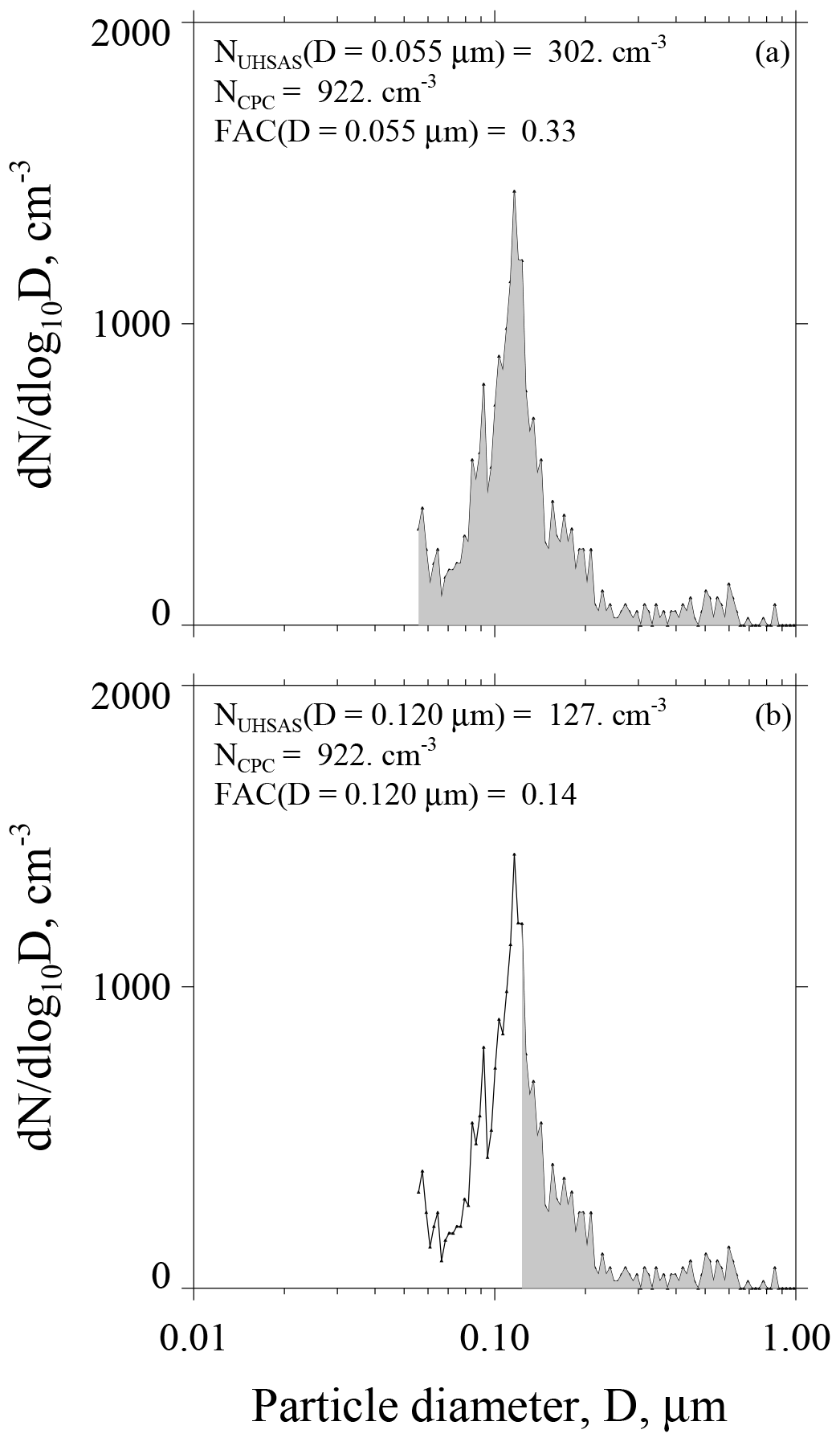
Figure 7Two portrayals of the ASD recorded during CCOPE at 08:45:03 UTC 5 June 2015. This ASD is also plotted in Fig. 4a. Gray area in both panels represents the aerosol concentration integrated from the indicated lower-limit D to 1 µm. (a) Figure legend has the size-integrated UHSAS concentration, calculated with lower-limit D set at 0.055 µm, the CPC concentration, and the fractional aerosol concentration (FAC). (b) Figure legend has the size-integrated UHSAS concentration, calculated with lower-limit D in Eq. (2) set at 0.120 µm, the CPC concentration, and the fractional aerosol concentration (FAC).
In a second step we interpret a FAC's lower-limit diameter as an upper-limit SS. We do this by applying a value for the kappa hygroscopicity parameter, which we set at κ=0.5, and by applying the kappa–Köhler formula of Petters and Kreidenweis (2007, their Eq. 6). This transformation from lower-limit D to upper-limit SS converts the FAC in Fig. 7a to FAC(SS = 0.41 %) and the FAC in Fig. 7b to FAC(SS = 0.13 %). We also evaluated how a range of the kappa parameter () translates to a range of SS. Our upper-limit κ comes from airborne measurements made over the southeastern Pacific Ocean during summer (Snider et al., 2017), and our lower-limit κ is the value recommended by Andreae and Rosenfeld (2008) for simulating aerosol indirect effects over continents.
The FACs in Fig. 7a–b are two of the many available from CCOPE. One way to aggregate these is to calculate a FAC for each of the 20 onshore trajectories. For example, if we select the lower-limit diameter at D=0.055 µm, plot numerator values (Eq. 5) vs. denominator values (Eq. 5), and fit with the equation , the “a” we derive is the FAC(D=0.055 µm) for a particular trajectory. FACs calculated in this way and with lower-limit D selected = 0.120 µm are presented in the seventh columns of Tables 3 and 4. Correlation coefficients presented in the eighth columns of these tables mostly exceed 0.5. By averaging over the 20 onshore trajectories, we calculated the overall averages presented at the bottom of the two tables. These overall averages are FAC(D=0.055 µm) = 0.35±0.13 (Table 3) and FAC(D=0.120 µm) = 0.13±0.07 (Table 4). This decrease in the FAC results because a larger lower-limit D (Eq. 5), implies a smaller numerator (Eq. 5) and thus a smaller FAC(D).
What we refer to as ensemble-averaged FACs were derived by selecting the numerator and denominator values represented in Eq. (5) from all 20 onshore trajectories. The selected data pairs were fitted in the manner discussed previously. In addition, upper and lower quartile values of the fitted slopes were calculated by applying the technique of Wolfe and Snider (2012; their Fig. 4d). We evaluated four ensemble-averaged FACs corresponding to four selected diameters (D=0.070, 0.095, 0.120, and 0.200 µm). The FAC at D=0.055 µm was eliminated from this analysis because Kupc et al. (2018) showed that UHSAS measurements, at D≤0.070 µm, are negatively biased. Results are presented as circles in Fig. 8 and vertical error bars represent the quartile range. Values plotted on the abscissa correspond to the four diameters, each transformed to an SS using the kappa–Köhler formula with κ=0.5, and horizontal error bars extend from most hygroscopic (κ=0.7), at the left-most limit, to least hygroscopic (κ=0.3), at the right-most limit.
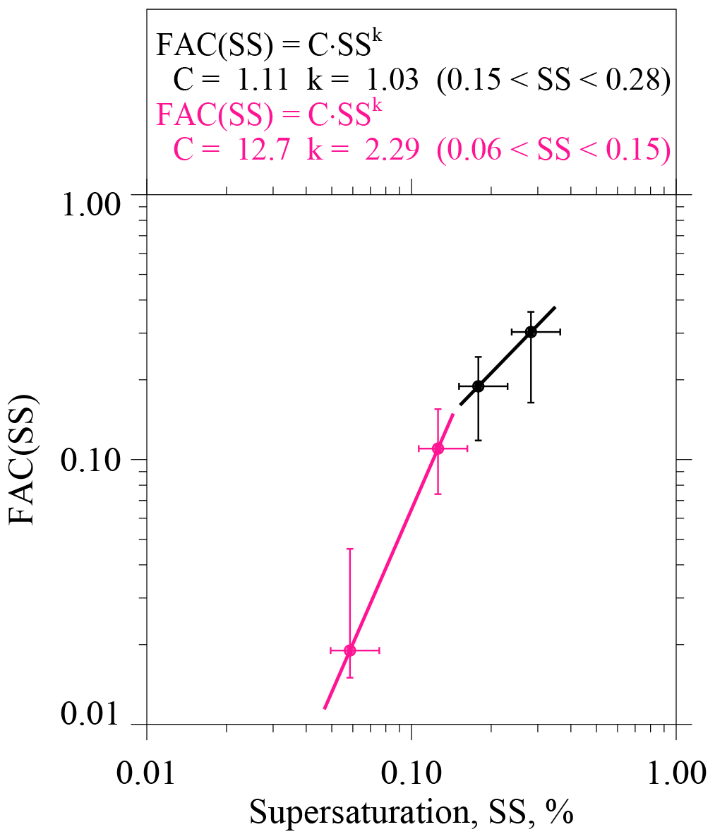
Figure 8Parameterized CCN activity spectrum derived using CPC and UHSAS measurements from the 20 onshore trajectories that arrived at the Arauco site between 29 May and 28 June 2015. Pink circles and the pink fit line are for lower-limit diameters set at 0.200 and 0.120 µm. Black circles and the black fit line are for lower-limit diameters set at 0.095 and 0.070 µm. Figure legend has power-law coefficients describing the parameterization; i.e., how FAC varies with SS.
In Fig. 8 we used power laws of the form FAC(SS) = C⋅SSk (i.e., the form commonly used to parameterize CCN activation spectra; Twomey, 1959) to fit the points. The change in the slope of the fit function, seen here at SS = 0.15 %, seems consistent with analyses, demonstrating that in polluted marine cloud conditions, albeit during summertime, the exponent “k” in the Twomey power fit function is ≥1 and ≤1 at SS < 0.1 % and SS > 0.1 %, respectively (Hudson and Nobel, 2014; data from the MASE project in their Fig. 1).
Our parameterized CCN activation spectrum (Fig. 8) is relevant to cloud–aerosol–precipitation modeling for several reasons. First, some numerical models treat SS as a prognostic variable and thus require initialization with a CCN activation spectrum (e.g., Khairoutdinov and Kogan, 2000). Similarly, some models initialize with a particle-size-dependent ASD function and use Köhler theory to derive a model-initializing CCN activation spectrum (e.g., Lebo et al., 2012). As described in these two references, these models initialize with a nonspecific CCN activation spectrum. If those models were used to investigate wintertime clouds and precipitation on the central Chilean Coast, our parameterization could be applied as a CCOPE-specific initialization. Second, since we have measurements of NCPC for the totality of CCOPE (Table 1), and we have shown how an ensemble-averaged CCN activation spectrum can be developed with NCPC as the input parameter – i.e., as – our parameterization can be used to estimate activation spectra for the complete CCOPE campaign. Third, model initiation with a specific CCN activation spectrum, as opposed to initialization with a regime-dependent droplet concentration (e.g., Thompson et al., 2004), is justified by sensitivities to cloud droplet activation reported in several publications (Cooper et al., 1997; Hudson and Yum, 1997; Snider et al., 2017).
An assumption implicit in our development is that particles were internally mixed within each of the four particle size classes. This seems justified by our use of HYSPLIT to conditionally sample (Sect. 3.1) and the fact that the sampled air masses were resident in the marine boundary layer for hours to days while subject to a variety of processes (Brownian coagulation and reactive uptake of SO2, among others) that produce aerosols consistent with the internal mixture assumption (Fierce et al., 2017). An aspect of our measurements also supports the internal mixture assumption. Figure 7b shows that number concentration corresponding to the 0.120 to 1 µm class is dominated by particles with diameters at the lower end of that class. Hence, the contribution of freshly emitted SSA particles, generally thought to size at dry diameters larger than 0.5 µm (Clarke et al., 2003; LS04), and with a κ=1.2 (Berg et al., 1998), is typically small. A different bias would result if particles with κ values smaller than the lower-limit value (κ=0.3) contributed significantly to the size-integrated concentration in Eq. (5). Burning biomass is an important source for such low-hygroscopicity particles (Carrico et al., 2005). Our conditional sampling (Sect. 3.1), combined with our filtering of the CPC and UHSAS measurements (Sect. 3.1 and Appendix B), reduces this concern.
4.5 Regression of N>0.5 and sea surface wind speed
As discussed in Sect. 3.2, N>0.5 represents the concentration of particles larger than 0.5 µm. We now support our conjecture that particles grouped into the N>0.5 subset are indeed SSA. We do this by analyzing the correlation between N>0.5 and sea surface wind speed (U). Section 3.1 explains how we used HYSPLIT to derive U.
Values of N>0.5, corresponding to the 18 sea surface trajectories (Sect. 3.1), are plotted against U in Fig. 9. Linear least-squares regression analysis with a model equation of the form was used to derive the coefficients No and aN (O'Dowd and Smith 1993; LS04). The fitted coefficients are No=0.15 cm−3 and aN=0.38 s m−1 and the derived function (black curve) is shown in Fig. 9. The dashed black curves represent the 95 % confidence interval (Romano, 1977; his Eq. 4.2.3.f). Also plotted (pink line) is the function derived by O'Dowd and Smith (1993) for dried SSA particles with a diameter between 0.38 and 0.84 µm. Given that the O'Dowd and Smith (1993) function (their Fig. 7a) is associated with statistical uncertainty comparable to what we estimate for our data set, we are only moderately confident that the function we derived is a consequence of wind-generated SSA. Two caveats require mentioning. First, a fraction of our data points (∼25 %) lie either above or below our confidence interval (Fig. 9). Meteorology can contribute to this variability, as when sea surface winds establish a SSA population, and the wind subsequently slacks or speeds up prior to advection onto the continent. This is expected because the atmospheric residence time of D∼0.5 µm particles, in the absence of precipitation, is several days (LS04, p. 76). Also, our unintentional sampling of particles generated over the continent is a concern. We have taken steps to eliminate those sources of contamination (Sect. 3.1 and Appendix B), but our methods are not foolproof.

Figure 9Averaged values of N>0.5 (±1 standard deviation) vs. HYSPLIT-derived averaged Us for the 18 sea surface trajectories that arrived at the Arauco site between 29 May and 28 June 2015. The black curve is the fit of the CCOPE data; dashed curves above and below the black curves are 95 % confidence intervals (Romano, 1977; his Eq. 4.2.3.f). The pink curve is the fit reported by O'Dowd and Smith (1993) for 0.38 µm < D<0.84 µm.
The measurements analyzed here are, to the best of our knowledge, the first to characterize aerosol microphysical properties on the central Chilean Pacific coast during winter. Since the measurement site was relatively close to a population center (Arauco, Chile), and an SO2-emitting paper mill, and because wood burning is an important source of residential heat in this region, we suspect that our measurements are influenced by these land sources. We mitigated against this by focusing on data collected during periods of onshore flow. Additional steps were taken to minimize contamination from land-based aerosol sources. These procedures are explained in Sects. 3.1, 4.2, Appendix B, and in the Supplement.
A point of comparison is the summertime measurements reported in HK98. Their data were collected during airborne sampling over the western Atlantic in air that had advected from the United States. HK98's averaged aerosol surface area (131±93 µm2 cm−3; their Table 2) is clearly larger than that for our 20 onshore trajectories (42±27 µm2 cm−3; results not shown). However, a more relevant comparison would be with low-altitude measurements made off the central Chilean Pacific coast during winter. As far as we know, the desired data set is not available. Values of aerosol surface area in the FT over the North and South Pacific are generally <10 µm2 cm−3 (Clarke, 1992), suggesting that even during onshore flow the Arauco site is affected by anthropogenic sources. We have assumed these sources are Chilean; however, a contribution from long range transport cannot be ruled out.
The larger winter-averaged CPC concentration at Arauco, compared to THD, is evidence for stronger continental contamination at the former. Since NCPC is a parameter in our parameterization of CCN activation spectra (Sect. 4.4), we conclude that cloud droplet concentrations in low-level marine clouds (stratocumulus) formed in the vicinity of Arauco are larger than in similar clouds near THD. If true, this conclusion would be the opposite of the general situation in southern Pacific boundary layer clouds, where cloud droplet concentrations are statistically lower than in their Northern Hemispheric counterparts (Bennartz, 2007). Relevant to this, Bennartz (2007) comments on a coast-normal droplet concentration gradient that is stronger on the central Chilean coast compared to the California and Oregon coast. We presume that the gradient exists because of the larger concentration of aerosols over continents (Andreae and Rosenfeld, 2008), and because of aerosol removal that occurs within and below marine stratocumulus clouds. In addition, Bennartz (2007) demonstrates that the coast-normal droplet concentration gradient is larger off the central Chilean coast, compared to the California and Oregon coast, in part because oceanic concentrations, ∼2000 km offshore, are generally smaller in the South Pacific compared to the North Pacific. Whether the Southern Hemispheric gradient is also enhanced by larger aerosol concentrations over coastal central Chile, compared to coastal California and Oregon, is an open question. Further analysis of the satellite retrievals analyzed by Bennartz (2007), with segregation into wintertime and summertime categories, as well as measurements conducted at an offshore island location or acquired using aircraft or ships, are needed to address this question.
Analyses presented here are based on condensation particle counter (CPC) measurements made during one winter season (June, July and August 2015) on the central Chilean Pacific coast (38∘ S). Also analyzed are aerosol size distribution measurements made with an ultra high sensitivity aerosol spectrometer (UHSAS). UHSAS measurements are available from 29 May to 28 June (Table 1). Limitations of this study are the proximity of the measurement site to a population center (Arauco, Chile) and an SO2-emitting paper mill, sampling of particles emitted from residences close to where our instruments were operated, and the incomplete drying of the sampled aerosol particles. This first attempt to make CPC and ASD measurements on the central Chilean Pacific coast during winter was exploratory, and our results should be considered preliminary.
We compared CPC-measured concentrations from the Arauco site to values acquired at the NOAA observatory Trinidad Head (THD) on the northern Pacific coast of California. The averaged CPC concentration is larger at the Arauco site and that difference is evident in an Arauco–THD comparison based on air arriving from all wind directions and from clean sector directions. In addition, we conditionally sampled UHSAS-measured size distributions and derived parameterized descriptions of sea salt aerosol (SSA) and cloud condensation nuclei (CCN) for periods of onshore flow. In these parameterizations the input parameters are, respectively, sea surface wind speed and CPC-measured concentration.
In the context of CCOPE, there are two precipitation regimes that impact the central Chilean Coast and the Nahuelbuta Range during winter (Massmann et al., 2017). The first of these have radar-derived echo tops at ∼2 km m.s.l. and produce rain by direct conversion of cloud droplets to rain drops. The second have higher echo tops, extending to temperatures colder than 0 ∘C and produce rain that is, at least in part, initiated by ice-phase processes. Investigation of the rain produced in the shallow regimes is an active area of research; it is thought that SSA and the CCN play important roles (Feingold et al., 1999; Gerber and Frick, 2012). The deep regimes form precipitating hydrometeors (ice particles) at cloud temperatures <0 ∘C. Again, aerosols play a role, but there are many facets to this, and first-order effects are not yet agreed on. Perhaps foremost is the role played by aerosol acting as ice nuclei. Measurement of an ice nuclei activation spectrum, development of an ice particle parameterization, and incorporation of the parameterization into a numerical model are needed to explore this dimension of the problem. Because they modulate cloud droplet size and the development of graupel and influence latent heating (e.g., Tao et al., 2012), the CCN and SSA likely also play a role in the deep regimes. Thus, we anticipate that modeling of both precipitation regimes will benefit from the CCN and SSA parameterizations presented here.
CCOPE CPC and UHSAS data and a data reader (Interactive Data Language, Harris Geospatial Solutions, Inc.) are available at http://www-das.uwyo.edu/~jsnider/CCOPE/ (last access: 27 September 2019).
Because the RH at the Arauco site was often in excess of 80 % (Fig. A1c), particles entering the sample tube (Sect. 2.2) were haze droplets (Rogers and Yau, 1989). As these haze droplets transit the sample tube they experience an increase in temperature, an RH decrease, and thus a decreased D. The lowest RH experienced by a haze droplet is at the point of detection where the aerosol temperature is presumed to be the internal “box temperature” measured by the UHSAS. The RH at this point is
where TU is the internal UHSAS temperature, es is saturation vapor pressure (temperature dependent), and RHA and TA are the ambient RH and temperature, respectively. In nearly all of the UHSAS sampling during CCOPE, the RHU was less than 60 % (Fig. A1d). This suggests that the haze droplets detected by the UHSAS were partially dried. Partial drying of the haze droplets is supported by calculations (Lewis and Schwartz, 2004; their Fig. 8) showing that a D=4 µm NaCl haze droplet reaches its equilibrium size (D=2 µm) in 0.1 s subsequent to a step-change of RH from 98 % to 80 %. Because 0.1 s is small relative to the average residence time of haze droplets within the sample tube (0.8 s), we ignored the possibility of a kinetic limitation to drying and we assumed that the haze droplets relaxed to their equilibrium size at RHU prior to the time they were detected. Since we do not know the chemical composition of the haze droplets, their equilibrium size is uncertain, but calculations corresponding to RHU=60 % and a haze droplet composed of sodium sulfate indicate that the equilibrium size is 30 % larger than the corresponding dry particle size (Snider et al., 2017; their Fig. A2b). Three factors interact to partially compensate for a size overestimate due to incomplete particle drying: (1) particle sizing performed by the UHSAS was calibrated using polystyrene latex particles (refractive index n=1.57 at λ=1.05 µm; Marx and Mulholland, 1983), (2) liquid water (n=1.32 at λ=1.05 µm; Irvine and Pollack, 1968) makes a significant contribution to the mass of a haze droplet at RH=60 % (here again we are assuming the above-mentioned sodium sulfate composition for the completely dried particle), and (3) assuming the same scattering intensity, an n=1.6 particle is 10 % smaller than an n=1.4 particle (Cai et al., 2008; their Fig. 1). Accepting the 10 % as an underestimate and the above-mentioned 30 % as an overestimate, we conclude that particle sizes reported by the UHSAS were overestimated by 20 %. We did not correct for this sizing bias.
Laboratory testing of the UHSAS and CPC is documented in Figs. A2a–b and in A3a–b. We evaluated consistency among measurements made with the UHSAS, the CPC, and a scanning mobility particle scanner (SMPS; TSI Inc., 2000b). In all of these tests, the RH of the test aerosols was <15 %. An example ASD derived using the UHSAS (pink) and the SMPS (black) is shown in Fig. A2a. In this test the three instruments (UHSAS, CPC and SMPS) were sampling mobility-selected ammonium sulfate particles with D=0.075 µm. The refractive index of this material at λ=1.05 µm is n=1.51 (Toon, 1976). It is evident that the mode diameter measured by the UHSAS is smaller than that reported by the SMPS (D=0.075 µm). This difference is qualitatively consistent with the smaller refractive index of the test material (ammonium sulfate), compared to the larger refractive index of the polystyrene latex particles used by the factory to calibrate the UHSAS (DMT, 2013). Figure A2b shows a test with D=0.71 µm polystyrene latex particles. As expected, the mode diameter in the UHSAS size distribution is in agreement with the mode size in the SMPS size distribution.
An additional feature of our laboratory testing is the multimodal structure in the SMPS size distribution at D<0.5 µm (Fig. A2b). This structure results because the particle diameter inferred by the SMPS depends on the physical diameter of the test particles and also on the test particle's charge state. The multimodal structure at D<0.5 µm corresponds to particles carrying five, four, three, and two fundamental charges but each with a physical diameter equal 0.71 µm. As stated in the previous paragraph, the latter is the diameter of the polystyrene test particles.
Figure A3a–b summarize all of the lab testing we conducted in support of CCOPE. In Fig. A3a, NUHSAS is plotted vs. NCPC for tests with D<0.2 µm and Fig. A3b has tests with D>0.2 µm. On average, concentrations differ by ±6 % in Fig. A3a (D<0.2 µm) and by ±10 % in Fig. A3b (D>0.2 µm).

Figure A1UHSAS internal temperature and ambient meteorological parameters at the Arauco site over a 4 d period. (a) Temperature inside the UHSAS. (b) Temperature measured on the meteorological tower. (c) RH measured on the meteorological tower. (d) Derived RH inside UHSAS.
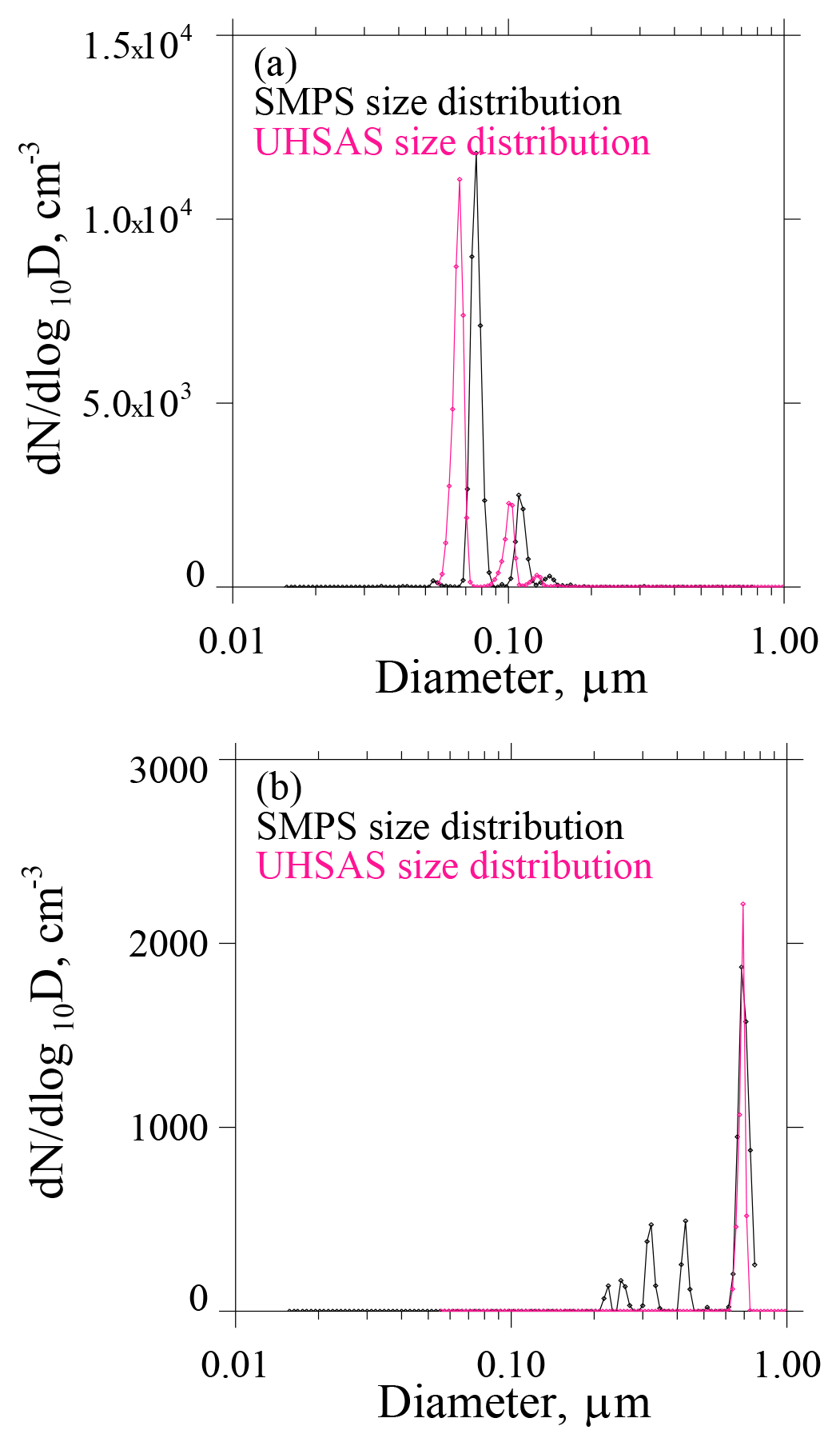
Figure A2(a) ASDs corresponding to mobility-selected D=0.075 µm ammonium sulfate test particles. (b) ASDs corresponding to mobility-selected D=0.71 µm polystyrene test particles.
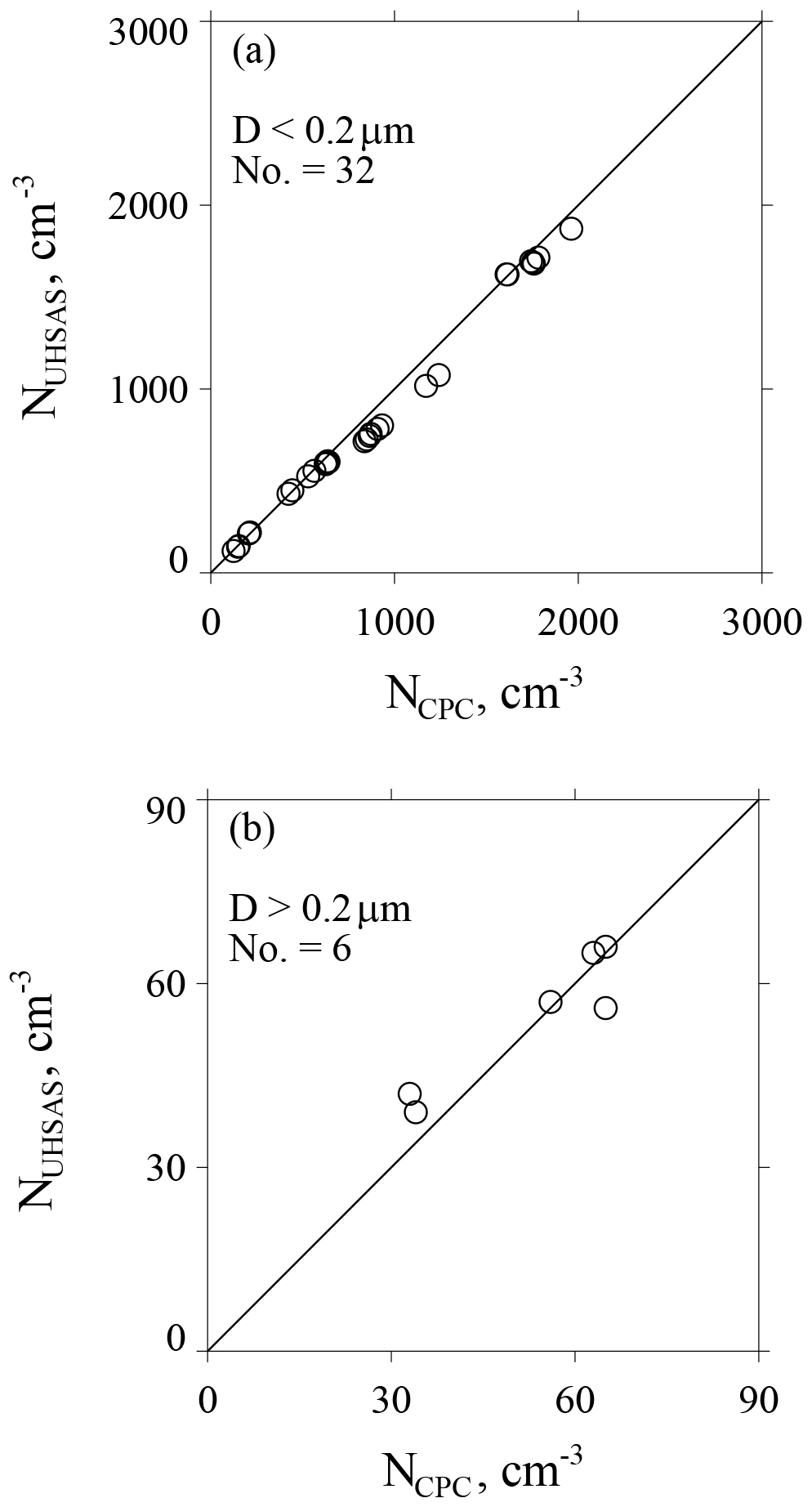
Figure A3(a) Size-integrated concentration from the UHSAS versus concurrent laboratory measurements of concentration from the CPC. Results are for mobility-selected ammonium sulfate test particles with D<0.2 µm. (b) As in (a) but for mobility-selected ammonium sulfate test particles with D>0.2 µm and for mobility-selected polystyrene latex test particles with D>0.2 µm.
For each of the onshore trajectories (Sect. 3.1), a 2 h segment, centered on the trajectory arrival time was analyzed. An example is in Fig. B1a–e. Figure B1a shows the sequence of CPC values sampled every second (i.e., 1 s samples referred to as fast NCPC), and Fig. B1b shows CPC values sampled every 10 s (i.e., 10 s samples referred to as slow NCPC). The following procedure was used to attenuate the narrow perturbations that were likely the result of local aerosol emissions (e.g., within the time interval indicated by vertical dashed lines in Fig. B1a, b, and d).
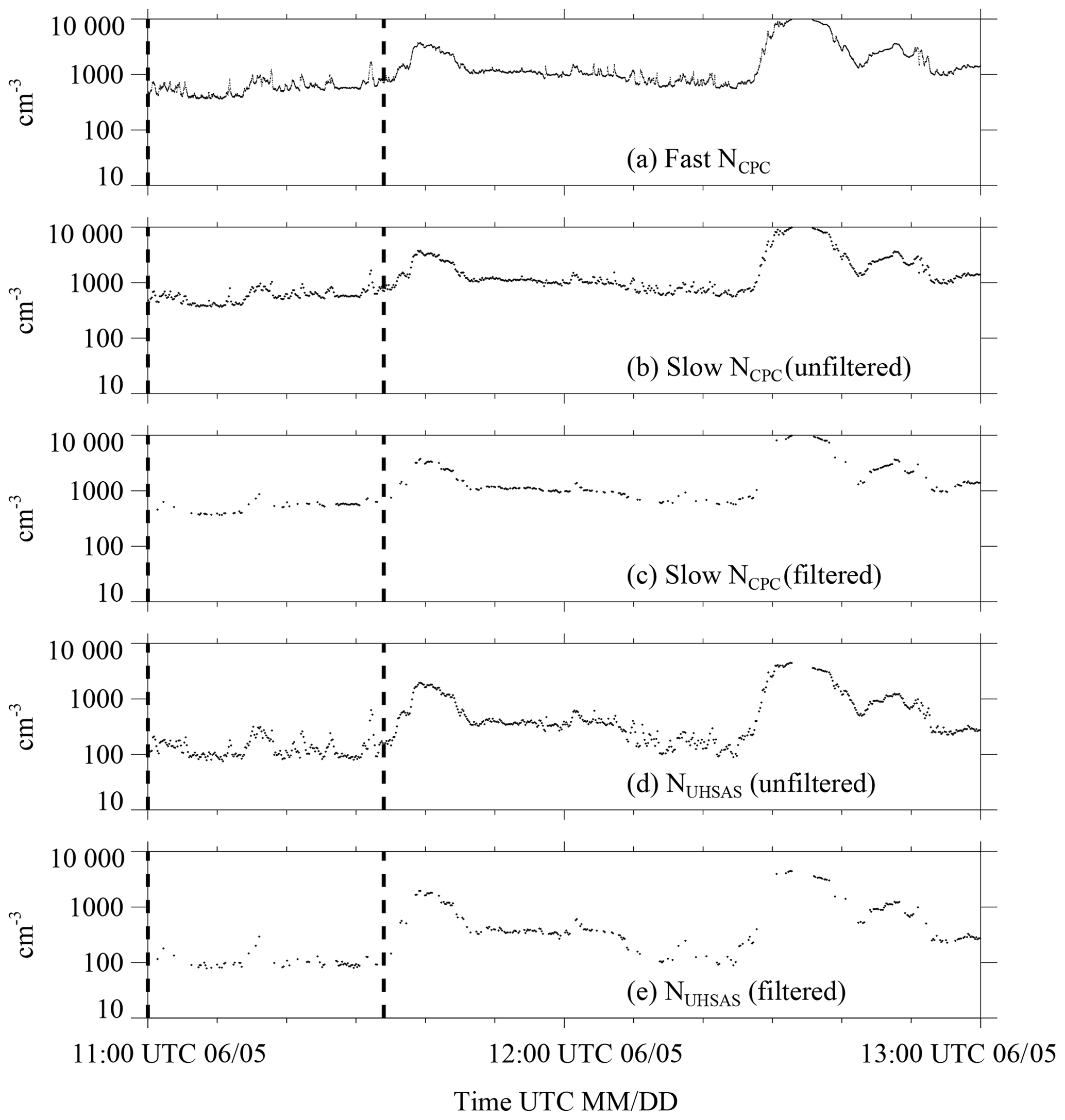
Figure B1Demonstration of the numerical filter. Measurements from one of the 20 onshore trajectories that arrived at the Arauco site between 29 May and 28 June. This trajectory arrival occurred at 12:00 UTC 5 June: (a) 1 s sampled CPC measurements, (b) 10 s sampled CPC measurements; (c) filtered 10 s CPC measurements, (d) 10 s UHSAS measurements of size-integrated concentration, and (e) filtered 10 s UHSAS measurements of size-integrated concentration.
First, the fast NCPC values were used to determine, for each 10 s of the sequence, a concentration relative standard deviation (σ∕〈x〉). Second, if the relative standard deviation was greater than 0.02, both the slow NCPC measurement (sampled once every 10 s) and the ASD measurement (also sampled once every 10 s; Table 1) were discarded. Figure B1c and e show the NCPC and NUHSAS sequences after application of the filter. These two filtered sequences (NCPC(filtered) and NUHSAS(filtered)) and the filtered values of aerosol surface area (SUHSAS), aerosol volume (VUHSAS), and D>0.5 µm concentration (N>0.5) are the focus of the bulk of our analysis.
The supplement related to this article is available online at: https://doi.org/10.5194/acp-19-12377-2019-supplement.
JRS, JRM, and DEK wrote successful proposals that funded this research. SLF, AKM, AM, and DEK performed the field measurements. RDG and AM provided logistical support during the field phase of the project. EA provided data from THD. SLF wrote her MS dissertation and this was adapted for this paper by JRS. All authors contributed to the editing of this paper.
The authors declare that they have no conflict of interest.
We thank Freddy Echeverría-Cabezas, for his assistance during CCOPE; Matthew Burkhart, for building the aerosol data acquisition system; Zhien Wang, for providing a graduate assistantship; Nicholas Mahon, for shipping logistics; and the Departamento de Geofísica at the Universidad de Concepción. This work was supported by the United States National Science Foundation Physical and Dynamic Meteorology Division under awards AGS-1522277 and AGS-1522939.
This research has been supported by the US National Science Foundation (grant nos. AGS-1522277, AGS-1522939).
This paper was edited by Veli-Matti Kerminen and reviewed by two anonymous referees.
Albrecht, B. A.: Aerosols, cloud microphysics, and fractional cloudiness, Science, 245, 1227–1230, 1989.
Andreae, M. O.: Correlation between cloud condensation nuclei concentration and aerosol optical thickness in remote and polluted regions, Atmos. Chem. Phys., 9, 543–556, https://doi.org/10.5194/acp-9-543-2009, 2009.
Andreae, M. O. and Rosenfeld, D.: Aerosol-cloud-precipitation interactions. Part 1. The nature and sources of cloud-active aerosols, Earth-Sci. Rev., 89, 13–41, 2008.
Arauco Woodpulp: available at: http://web.arauco.cl/_file/file_3382_pulp catalog.pdf (last access: 16 December 2018), 2010.
Bennartz, R.: Global assessment of marine boundary layer cloud droplet number concentration from satellite, J. Geophys. Res., 112, D02201, https://doi.org/10.1029/2006JD007547, 2007.
Berg, O. H., Swietlicki, E., and Krejci, R.: Hygroscopic growth of aerosol particles in the marine boundary layer over the Pacific and Southern Oceans during the First Aerosol Characterization Experiment (ACE 1), J. Geophys. Res., 103, 16535–16545, 1998.
Birmili, W., Wiedensohler, A., Heintzenberg, J., and Lehmann, K.: Atmospheric particle number size distribution in central Europe: Statistical relations to air masses and meteorology, J. Geophys. Res.-Atmos., 106, 32005–32018, 2001.
Boucher, O., Randall, D., Artaxo, P., Bretherton, C., Feingold, G., Forster, P., Kerminen, V.-M., Kondo, Y., Liao, H., Lohmann, U., Rasch, P., Satheesh, S. K., Sherwood, S., Stevens, B., and Zhang, X. Y.: Clouds and Aerosols, in: Climate Change 2013: The Physical Science Basis. Contribution of Working Group I to the Fifth Assessment Report of the Intergovernmental Panel on Climate Change, edited by: Stocker, T. F., Qin, D., Plattner, G.-K., Tignor, M., Allen, S. K., Boschung, J., Nauels, A., Xia, Y., Bex, V., and Midgley, P. M., Cambridge University Press, Cambridge, UK, 2013.
Brechtel, F. J., Kreidenweis, S. M., and Swan, H. B.: Air mass characteristics, aerosol particle number concentrations, and number size distributions at Macquarie Island during the First Aerosol Characterization Experiment (ACE 1), J. Geophys. Res.-Atmos., 103, 16351–16367, 1998.
Cai, Y., Montague, D. C., Mooiweer-Bryan, W., and Deshler, T.: Performance characteristics of the ultra high sensitivity aerosol spectrometer for particles between 55 and 800 nm: Laboratory and field Studies, J. Aerosol Sci., 39, 759–769, 2008.
Cai, Y., Snider, J. R., and Wechsler, P.: Calibration of the passive cavity aerosol spectrometer probe for airborne determination of the size distribution, Atmos. Meas. Tech., 6, 2349–2358, https://doi.org/10.5194/amt-6-2349-2013, 2013.
Carrico, C. M., Kreidenweis, S. M., Malm, W. C., Day, D. E., Lee, T., Carrillo, J., McMeeking, G. R., and Collett, J. L.: Hygroscopic growth behavior of a carbon-dominated aerosol in Yosemite National Park, Atmos. Environ., 39, 1393–1404, 2005.
Clarke, A.: Atmospheric Nuclei in the Remote Free-Troposphere, J. Atmos. Chem., 14, 479–488, 1992.
Clarke, A., Kapustin, V., Howell, S., Moore, K., Lienert, B., Masonis, S., Anderson, T., and Covert, D.: Sea-salt size distribution from breaking waves: Implications for marine aerosol production and optical extinction measurements during SEAS, J. Atmos. Ocean. Technol., 20, 1362–1374, 2003.
Cooper, W. A., Bruintjes, R. T., and Mather, G. K.: Calculations pertaining to hygroscopic seeding with flares, J. Appl. Meteorol., 36, 1449–1469, 1997.
Covert, D. S., Kapustin, V. N., Quinn, P. K., and Bates, T. S.: New particle formation in the marine boundary layer, J. Geophys. Res., 97, 20581–20589, https://doi.org/10.1029/92JD02074, 1992.
Dall'Osto, M., Ceburnis, D., Martucci, G., Bialek, J., Dupuy, R., Jennings, S. G., Berresheim, H., Wenger, J., Healy, R., Facchini, M. C., Rinaldi, M., Giulianelli, L., Finessi, E., Worsnop, D., Ehn, M., Mikkilä, J., Kulmala, M., and O'Dowd, C. D.: Aerosol properties associated with air masses arriving into the North East Atlantic during the 2008 Mace Head EUCAARI intensive observing period: an overview, Atmos. Chem. Phys., 10, 8413–8435, https://doi.org/10.5194/acp-10-8413-2010, 2010.
Diesch, J.-M., Drewnick, F., Zorn, S. R., von der Weiden-Reinmüller, S.-L., Martinez, M., and Borrmann, S.: Variability of aerosol, gaseous pollutants and meteorological characteristics associated with changes in air mass origin at the SW Atlantic coast of Iberia, Atmos. Chem. Phys., 12, 3761–3782, https://doi.org/10.5194/acp-12-3761-2012, 2012.
DMT: Ultra High Sensitivity Aerosol Spectrometer (UHSAS) Operator Manual, Boulder, CO, 2013.
Feingold, G., Cotton, W. R., Kreidenweis, S. M., and Davis, J. T.: The Impact of Giant Cloud Condensation Nuclei on Drizzle Formation in Stratocumulus: Implications for Cloud Radiative Properties, J. Atmos. Sci., 56, 4100–4117, 1999.
Fierce, L., Riemer, N., and Bond, T. C.: Toward Reduced Representation of Mixing State for Simulating Aerosol Effects on Climate, B. Am. Meteorol. Soc., 98, 971–980, https://doi.org/10.1175/BAMS-D-16-0028.1, 2017.
Fults, S.: Aerosol measurements during the Central Chilean Orographic Precipitation Experiment, MSc Thesis, Department of Atmospheric Science, University of Wyoming, 2016.
Garreaud, R., Falvey, M., and Montecinos, A.: Orographic precipitation in coastal southern Chile: Mean distribution, temporal variability, and linear contribution, J. Hydrometeorol., 17, 1185–1202, https://doi.org/10.1175/JHM-D-15-0170.1, 2016.
Gerber, H. and Frick, G.: Drizzle rates and large sea-salt nuclei in small cumulus, J. Geophys. Res., 117, D01205, https://doi.org/10.1029/2011JD016249, 2012.
Gras, J. L.: Baseline atmospheric condensation nuclei at Cape Grim 1977–1987, J. Atmos. Chem., 11, 89–106, 1990.
Gras, J. L.: CN, CCN and particle size in Southern Ocean air at Cape Grim, J. Atmos. Res., 35, 233–251, 1995.
Hansen, J.: The Faustian Bargain: Humanity's Own Trap, Storms of My Grandchildren, Bloomsbury, New York, NY, 320 pp., 2009.
Havlicek, L. L. and Crain, R. D.: Practical Statistics for the Physical Sciences, American Chemical Society, Washington, DC, 512 pp., 1988.
Hegg, D. A. and Kaufman, Y. J.: Measurements of the relationship between submicron aerosol number and volume concentration, J. Geophys. Res., 103, 5671–5678, 1998.
Hinds, W. C.: Aerosol Technology: Properties, Behavior and Measurement of Airborne Particles, John Wiley & Sons, INC, New York, NY, 483 pp., 1999.
Hoppel, W. A., Frick, G. M., Fitzgerald, J. W., and Larson, R. E.: Marine boundary layer measurements of new particle formation and the effects nonprecipitating clouds have, J. Geophys. Res., 99, 14443–14459, 1994.
Hudson, J. G. and Nobel, S.: CCN and vertical velocity influences on droplet concentrations and supersaturations in clean and polluted stratus clouds, J. Atmos. Sci., 71, 312–331, https://doi.org/10.1175/JAS-D-13-086.1, 2014.
Hudson, J. G. and Yum, S.: Droplet spectral broadening in marine stratus, J. Atmos. Sci., 54, 2642–2654, 1997.
Hudson, J. G., Noble, S., and Tabor, S.: Cloud supersaturations from CCN spectra Hoppel minima, J. Geophys. Res.-Atmos., 120, 3436–3452, https://doi.org/10.1002/2014JD022669, 2015.
International Civil Aviation Organization (ICAO): Manual of the ICAO Standard Atmosphere: extended to 80 kilometres (262 500 feet), 3rd Edn., ISBN 92-9194-004-6, 1993.
Irvine, W. M. and Pollack, J. B.: Infrared optical properties of water and ice spheres, Icarus, 8, 324–360, 1968.
Khairoutdinov, M. and Kogan, Y.: A new cloud physics parameterization in a large-eddy simulation model of marine stratocumulus, Mon. Weather Rev., 128, 229–243, 2000.
Kupc, A., Williamson, C., Wagner, N. L., Richardson, M., and Brock, C. A.: Modification, calibration, and performance of the Ultra-High Sensitivity Aerosol Spectrometer for particle size distribution and volatility measurements during the Atmospheric Tomography Mission (ATom) airborne campaign, Atmos. Meas. Tech., 11, 369–383, https://doi.org/10.5194/amt-11-369-2018, 2018.
Lebo, Z. J., Morrison, H., and Seinfeld, J. H.: Are simulated aerosol-induced effects on deep convective clouds strongly dependent on saturation adjustment?, Atmos. Chem. Phys., 12, 9941–9964, https://doi.org/10.5194/acp-12-9941-2012, 2012.
Lewis, E. R. and Schwartz, S. E.: Sea Salt Aerosol Production: Mechanisms, Methods, Measurements, and Models, American Geophysical Union, 413 pp., Washington, DC, 2004.
Marx, E. and Mulholland, G. W.: Size and refractive index determination of single polystyrene spheres, J. Res. Na. Bur. Stand., 88, 321–338, 1983.
Massmann, A. K., Minder, J. R., Garreaud, R. D., Kingsmill, D. E., Valenzuela, R. A., Montecinos, A., Fults, S. L., and Snider, J. R.: The Chilean Coastal Orographic Precipitation Experiment: Observing the Influence of Microphysical Rain Regimes on Coastal Orographic Precipitation, J. Hydrometeorol., 18, 2723–2743, https://doi.org/10.1175/JHM-D-17-0005.1, 2017.
McCoy, D. T., Hartmann, D. L., and Grosvenor, D. P.: Observed Southern Ocean Cloud Properties and Shortwave Reflection. Part I: Calculation of SW Flux from Observed Cloud Properties, J. Climate, 27, 8836–8857, https://doi.org/10.1175/JCLI-D-14-00287.1, 2014.
McMurry, P. H., Wang, X., Park, K., and Ehara, K.: The relationship between mass and mobility for atmospheric particles: A new Technique for measuring particle density, Aerosol Sci. Tech., 36, 227–238, 2002.
NOAA: HYSPLIT Trajectory Model, NOAA Air Resources Laboratory, Silver Spring, MD, available at: https://ready.arl.noaa.gov/HYSPLIT.php, last access: 1 August 2016.
O'Dowd, C. D. and Smith, M. H.: Physicochemical properties of aerosols over the Northeast Atlantic: evidence for wind-speed-related submicron sea-salt aerosol production, J. Geophys. Res., 98, 1137–1149, 1993.
Petters, M. D. and Kreidenweis, S. M.: A single parameter representation of hygroscopic growth and cloud condensation nucleus activity, Atmos. Chem. Phys., 7, 1961–1971, https://doi.org/10.5194/acp-7-1961-2007, 2007.
Petters, M. D., Snider, J. R., Stevens, B., Vali, G., Faloona, I., and Russell, L. M.: Accumulation mode aerosol, pockets of open cells, and particle nucleation in the remote subtropical Pacific marine boundary layer, J. Geophys. Res.-Atmos., 111, 1–15, 2006.
Raes, F., Van Dingenen, R., Cuevas, E., Van Velthoven, P. F. J., and Prospero, J. M.: Observations of aerosols in the free troposphere and marine boundary layer of the subtropical Northeast Atlantic: Discussion of processes determining their size distribution, J. Geophys. Res., 102, 21315, https://doi.org/10.1029/97JD01122, 1997.
Rogers, R. R. and Yau, M. K.: A Short Course in Cloud Physics, 3rd Edn., Permagon Press, Oxford, UK, 304 pp., 1989.
Romano, A.: Applied Statistics for Science and Industry, Allyn and Bacon Inc., Boston, MA, 385 pp., 1977.
Schwartz, S. E.: Are global cloud albedo and climate controlled by marine phytoplankton?, Nature, 336, 441–445, 1988.
Snider, J. R., Leon, D., and Wang, Z.: Droplet Concentration and Spectral Broadening in Southeast Pacific Stratocumulus, J. Atmos. Sci., 74, 719–749, 2017.
Tao, W. K., Chen, J. P., Li, Z., Wang, C., and Zhang, C.: Impact of aerosols on convective clouds and precipitation, Rev. Geophys., 50, RG2001, https://doi.org/10.1029/2011RG000369, 2012.
Thompson, G., Rasmussen, R. M., and Manning, K.: Explicit forecasts of winter precipitation using an improved bulk microphysics scheme. Part I: Description and sensitivity analysis, Mon. Weather Rev., 132, 519–542, 2004.
Toon, O. B.: The optical constants of several atmospheric aerosol species: Ammonium sulfate, aluminum oxide, and sodium chloride, J. Geophys. Res., 81, 5733–5748, 1976.
TSI Inc.: Condensation Particle Counter Instruction Manual, St. Paul, Minnesota, 2000a.
TSI Inc.: Model 3080 Electrostatic Classifier Instruction Manual, St. Paul, Minnesota, 2000b.
Twomey, S.: The nuclei of natural cloud formation part II: The supersaturation in natural clouds and the variation of cloud droplet concentration, Geofis. Pura Appl., 43, 243–249, 1959.
Twomey, S.: Pollution and the Planetary Albedo, Atmos. Environ., 8, 1251–56, 1974.
van Dingenen, R., Virkkula, A. O., Raes, F., Bates, T. S., and Wiedensohler, A.: A simple non linear analytical relationship between aerosol accumulation number and sub-micron volume, explaining their observed ratio in the clean and polluted marine boundary layer, Tellus B, 52, 439–451, 2000.
Wiedensohler, A., Orsini, D., Covert, D. S., Coffmann, D., Cantrell, W., Havlicek, M., Brechtel, F. J., Russell, L. M., Weber, R. J., Gras, J., Hudson, J. G., and Litchy, M.: Intercomparison Study of the Size-Dependent Counting Efficiency of 26 Condensation Particle Counters, Aerosol Sci. Tech., 27, 224–242, https://doi.org/10.1080/02786829708965469, 1997.
Wolfe, J. P. and Snider, J. R.: A relationship between reflectivity and snow rate for a high-altitude S-band radar, J. Appl. Meteorol. Clim., 51, 1111–1128, 2012.
Yum, S. S. and Hudson, J. G.: Wintertime/summertime contrasts of cloud condensation nuclei and cloud microphysics over the Southern Ocean, J. Geophys. Res., 109, 1–14, 2004.
The CPC minimum detectable diameters we report are in fact diameters at which a CPC detects particles with efficiency = 50 %. The CPC detection efficiency is a steep function of particle diameter (Wiedensohler et al., 1997).
Trajectory starting altitude was set at 60 m m.s.l. (5 m above the Arauco site).
In the case of ambient particles containing hygroscopic materials, density values range between 1.5 and 1.8 g cm−3 (McMurry et al., 2002).