NH<sub>3</sub> emissions from large point sources derived from CrIS and IASI satellite observations

Dammers, Enrico; McLinden, Chris A.; Griffin, Debora; Shephard, Mark W.; Van Der Graaf, Shelley; Lutsch, Erik; Schaap, Martijn; Gainairu-Matz, Yonatan; Fioletov, Vitali; Van Damme, Martin; Whitburn, Simon; Clarisse, Lieven; Cady-Pereira, Karen; Clerbaux, Cathy; Coheur, Pierre Francois; Erisman, Jan Willem

doi:https://doi.org/10.5194/acp-19-12261-2019

Articles | Volume 19, issue 19

https://doi.org/10.5194/acp-19-12261-2019

Articles | Volume 19, issue 19

Research article

02 Oct 2019

Research article |

| 02 Oct 2019

NH₃ emissions from large point sources derived from CrIS and IASI satellite observations

Enrico Dammers, Chris A. McLinden, Debora Griffin, Mark W. Shephard, Shelley Van Der Graaf, Erik Lutsch, Martijn Schaap, Yonatan Gainairu-Matz, Vitali Fioletov, Martin Van Damme, Simon Whitburn, Lieven Clarisse, Karen Cady-Pereira, Cathy Clerbaux, Pierre Francois Coheur, and Jan Willem Erisman

Abstract

Ammonia (NH₃) is an essential reactive nitrogen species in the biosphere and through its use in agriculture in the form of fertilizer (important for sustaining humankind). The current emission levels, however, are up to 4 times higher than in the previous century and continue to grow with uncertain consequences to human health and the environment. While NH₃ at its current levels is a hazard to environmental and human health, the atmospheric budget is still highly uncertain, which is a product of an overall lack of measurements. The capability to measure NH₃ with satellites has opened up new ways to study the atmospheric NH₃ budget. In this study, we present the first estimates of NH₃ emissions, lifetimes and plume widths from large ( $> \sim 5$ kt yr⁻¹) agricultural and industrial point sources from Cross-track Infrared Sounder (CrIS) satellite observations across the globe with a consistent methodology. The same methodology is also applied to the Infrared Atmospheric Sounding Interferometer (IASI) (A and B) satellite observations, and we show that the satellites typically provide comparable results that are within the uncertainty of the estimates. The computed NH₃ lifetime for large point sources is on average 2.35±1.16 h. For the 249 sources with emission levels detectable by the CrIS satellite, there are currently 55 locations missing (or underestimated by more than an order of magnitude) from the current Hemispheric Transport Atmospheric Pollution version 2 (HTAPv2) emission inventory and only 72 locations with emissions within a factor of 2 compared to the inventories. The CrIS emission estimates give a total of 5622 kt yr⁻¹, for the sources analyzed in this study, which is around a factor of ∼2.5 higher than the emissions reported in HTAPv2. Furthermore, the study shows that it is possible to accurately detect short- and long-term changes in emissions, demonstrating the possibility of using satellite-observed NH₃ to constrain emission inventories.

Download & links

Article (PDF, 7751 KB)

Supplement (163 KB)

Download & links

Article (7751 KB)
Supplement (163 KB)
BibTeX
EndNote

How to cite

How to cite.

Dammers, E., McLinden, C. A., Griffin, D., Shephard, M. W., Van Der Graaf, S., Lutsch, E., Schaap, M., Gainairu-Matz, Y., Fioletov, V., Van Damme, M., Whitburn, S., Clarisse, L., Cady-Pereira, K., Clerbaux, C., Coheur, P. F., and Erisman, J. W.: NH₃ emissions from large point sources derived from CrIS and IASI satellite observations, Atmos. Chem. Phys., 19, 12261–12293, https://doi.org/10.5194/acp-19-12261-2019, 2019.

Dates

Received: 13 May 2019 – Discussion started: 05 Jun 2019 – Revised: 19 Aug 2019 – Accepted: 21 Aug 2019 – Published: 02 Oct 2019

1 Introduction

Ammonia (NH₃) is one of the most important reactive nitrogen species in the biosphere and essential for sustaining humankind through its use in agriculture in the form of fertilizer. However, at the current emission levels, which are up to 4 times higher than in the previous century and which continue to grow with uncertain consequences (Holland et al., 1999; Fowler et al., 2013; Battye et al., 2017), which raises major environmental and health challenges (Sutton et al., 2009; Rockstrom et al., 2009). Through deposition, NH₃ can cause eutrophication and acidification (Erisman et al., 2007; EEA-European Environment Agency, 2014), which can lead to a reduction of biodiversity in vulnerable ecosystems (Bobbink et al., 2010). On the other hand, through fertilization of ecosystems, deposited NH₃ and other reactive nitrogen species play an important role in the sequestration of carbon dioxide (Oren et al., 2001; de Vries et al., 2014). NH₃ reacts rapidly with acidic gases, forming ammonium nitrate and ammonium sulfate, which combined add up to 50 % of the mass of fine particulate matter (Schaap et al., 2004; Seinfeld and Pandis, 2012). Particulate matter is shown to have impact on human health, shortening human life expectancy and affecting pregnancy outcomes (Pope III et al., 2002, 2009; Stieb et al., 2012; Lelieveld et al., 2015; Giannakis et al., 2019). Furthermore, particulate matter impacts global climate change directly through the change in radiative forcing and indirectly through its effects on cloud formation (Adams et al., 2001; Myhre et al., 2013).

While measures to reduce NO_x and SO₂ emissions have had a significant and measurable effect (Krotkov et al., 2016; Lamsal et al., 2015), emission control measures for NH₃ have not sufficiently been implemented, and the efficiency of the proposed measures is uncertain. Several studies (Erisman and Schaap, 2004; Xu et al., 2017) have shown the importance of similar emission controls for NH₃. Recently, though, there has been significant debate on the quality of both modeled emissions and observed concentrations, as modeled long-term trends do not match observed trends. Over the last decade, several studies have focused on solving this discrepancy but have been unsuccessful to date (Yao and Zhang, 2016; Van Zanten et al., 2017; Wichink Kruit et al., 2017). One of the problems is the lack of dense and precise measurement networks. NH₃ concentrations are highly variable in time and space, as shown by in situ and aircraft observations. With estimated lifetimes of a few hours up to a few days, a wide distribution of measurements, both spatially and temporally, is needed to understand the processes and infer a representative atmospheric budget. Globally, there are only a few measurement networks, with few consisting of more than a small number (>5) of locations (e.g., the MAN network; Lolkema et al., 2015) and even fewer with a consistent measurement record or providing vertical profiles (Erisman et al., 1988; Dammers et al., 2017 a; Tevlin et al., 2017; Y. Zhang et al., 2018). This makes it hard to study and resolve the discrepancy in the trends. Furthermore, most measurements are performed at a coarse temporal resolution (up to monthly averages), while most of the atmospheric processes, such as emissions, deposition and chemical conversion to particulate matter (PM_2.5), take place on timescales of minutes to hours.

The availability of satellite observations in recent years has provided global coverage of NH₃, opening up new ways to study the atmospheric NH₃ budget. Instruments such as the Tropospheric Emission Spectrometer (TES; Beer et al., 2008; Shephard et al., 2011), the Atmospheric Infrared Sounder (AIRS; Warner et al., 2016), the Infrared Atmospheric Sounding Interferometer (IASI; Clarisse et al., 2009; Coheur et al., 2009; Van Damme et al., 2014 a) and the Cross-track Infrared Sounder (CrIS; Shephard and Cady-Pereira, 2015) have shown that it is possible to retrieve NH₃ from spectra obtained by satellites. These satellite NH₃ observations have greatly improved our understanding of its distribution. Studies showed the global distribution of NH₃ measured one or two times per day (Van Damme et al., 2014 a; Shephard and Cady-Pereira, 2015) can reveal seasonal cycles and distributions for regions where measurements are commonly sparse or unavailable (Warner et al., 2017; Van Damme et al., 2015; Whitburn et al., 2015, 2016 b). Several studies have compared satellite measured to modeled NH₃ concentrations showing an overall underestimation of the modeled concentrations in North America (Heald et al., 2012; Nowak et al., 2012; Zhu et al., 2013; Schiferl et al., 2014, 2016; Lonsdale et al., 2017), Europe (Van Damme et al., 2014 b; Wichink Kruit et al., 2017) and China (L. Zhang et al., 2018), potentially due to an underestimation of the emissions. The atmospheric lifetime of NH₃ is highly uncertain as most of the commonly used ground-based instruments have a temporal resolution that is too coarse to resolve it. There are only a few estimates reported in literature, ranging from several hours up to 2 d, obtained either by analyzing short- or long-range transport of fire plumes (Yokelson et al., 2009; R'Honi et al., 2013; Whitburn et al., 2015; Lutsch et al., 2016; Adams et al., 2019) or through model estimates, such as by Dentener and Crutzen (1994).

Satellite observations have been successfully used for direct estimates of emissions and lifetimes of several species (e.g., SO₂, NO_x, CO₂, CO and NH₃) for single anthropogenic point sources (Martin, 2008; Streets et al., 2013; Fioletov et al., 2015; Nassar et al., 2017) and biomass burning (Mebust et al., 2011; Castellanos et al., 2015; Whitburn et al., 2015; Adams et al., 2019), as well as for estimating emissions for multiple sources at the same time (Fioletov et al., 2017). A multitude of approaches exist: simple box models (Jacob, 1999; Hickman et al., 2018; Van Damme et al., 2018), methods that take the wind direction into account (Beirle et al., 2011; Pommier et al., 2013) and more complete methods that account for diffusion and plume shape (Fioletov et al., 2011; de Foy et al., 2014; McLinden et al., 2016; Nassar et al., 2017). In the case of NH₃, there are several studies that report emission estimates based on satellite observations (R'Honi et al., 2013; Whitburn et al., 2015, 2016 b; Van Damme et al., 2018; Hickman et al., 2018; Adams et al., 2019). However, due to the low signal-to-noise ratio of single observations and the relatively coarse spatial resolution, only a few studies have used direct emission estimates from satellite observations (e.g., Van Damme et al., 2018; Hickman et al., 2018; Adams et al., 2019). Other studies have commonly used model inversions in various forms (Zhu et al., 2013; L. Zhang et al., 2018). Independent of the methods used, most studies indicate a regional and national underestimation of up to several orders of magnitude for both anthropogenic and natural emissions in most current inventories.

Here, we derive and compare NH₃ emissions and, for the first time, lifetimes of globally distributed industrial and agricultural emission sources based on the independent observations of NH₃ by CrIS and IASI. We use the complete datasets of IASI-A, IASI-B and CrIS to give estimates for both the 2008–2017 (IASI-A) and 2013–2017 (CrIS, IASI-A and -B) intervals. We show that all instruments provide comparable emission estimates and similar interannual variability. In Sect. 2, we describe the datasets and the methods, and estimate the uncertainty of the method used in this study. In Sect. 3, we describe the results, starting with the fitted lifetime and the plume spread (σ), which will be used to constrain the final emission fits given in Sect. 3.2. Furthermore, Sect. 3.3 describes the temporal variations in the emission estimates. Finally, in Sect. 4, we summarize and discuss the results.

2 Datasets and method

2.1 Satellite products

2.1.1 CrIS

The CrIS instrument is aboard the Suomi-NPP platform launched in October 2011. It orbits the Earth in a Sun-synchronous orbit, with twice daily global coverage, crossing the Equator at 13:30 and 01:30 local solar time (LST). The instrument covers a wide swath of up to 2200 km width with circular pixels that have a diameter of 14 km at nadir. In this study, we use version 1.5 data of the CrIS – fast physical retrieval (FPR)-NH₃ product (see Shephard and Cady-Pereira, 2015 and Shephard et al., 2019 for more details). The CrIS-FPR retrieval is a physical retrieval based on the optimal estimation method (Rodgers, 2000) that uses the fast optimal spectral sampling (OSS)-CrIS (Moncet et al., 2008) forward model to minimize the residual between the measured and simulated spectra. The previous version of the CrIS-NH₃ product (version 1.3) has been compared with ground-based Fourier transform infrared spectroscopy (FTIR) observations and showed good performance (Dammers et al., 2017 b) with correlations of r∼0.8 and a slope of 1.02. The validation study indicated that for total columns greater than 10×10¹⁵ molecules cm⁻², CrIS-FPR values have a small ∼ 0 %–5 % difference with a standard deviation (SD) of 25 % up to 50 %, which is within the FTIR- and CrIS-estimated retrieval uncertainties. For the total columns smaller than 10×10¹⁵ molecules cm⁻², the difference is larger, with a positive bias of 2.4×10¹⁵ ( $\pm 5.5 \times 10^{15}$ ) molecules cm⁻², equivalent to a relative difference of around 50 % (±100 %). This larger relative bias can occur for observations close to the detection limit of the CrIS instrument, which conservatively is about 0.9 ppb, as reported by Shephard and Cady-Pereira (2015), but under ideal conditions reaches down to ∼0.3 ppb (Kharol et al., 2018) (assuming that 1 ppb is equal to a total column of $2 \pm 1 \times 10^{15}$ molecules cm⁻², this leads to a detection limit of $1.8 \pm 0.9 \times 10^{15}$ molecules cm⁻²). Note, version 1.5 of the CrIS NH₃ retrievals only contains values that have a detectable NH₃ spectral signal; thus, in regions where there is a significant fraction of the values below the detection limit, the mean values can be biased towards values at or above the detection limit (see Shephard et al., 2019 for more details). For this study, only daytime observations between January 2013 and December 2018 are used. Furthermore, only observations with a quality flag of 5 are used (Shephard et al., 2019); the dataset was further filtered by only allowing observations that have a signal-to-noise ratio >2 (which in practice means that all observations with the unpolluted a priori are filtered out), degrees of freedom >0.8 and a thermal contrast $> - 2$ K to filter out anomalous values due to thin clouds, very cold surfaces and observations with low information content. Figure 1 shows a 5-year mean (2013–2017) of CrIS total column concentrations on a 0.05^∘ × 0.05^∘ grid. The original CrIS total column data have been smoothed by the pixel-averaging technique (Fioletov et al., 2011, 2015) with a 0.15^∘ radius which is comparable in size to the pixel footprints. The black circles indicate the source locations used in this study with successful emission estimates.

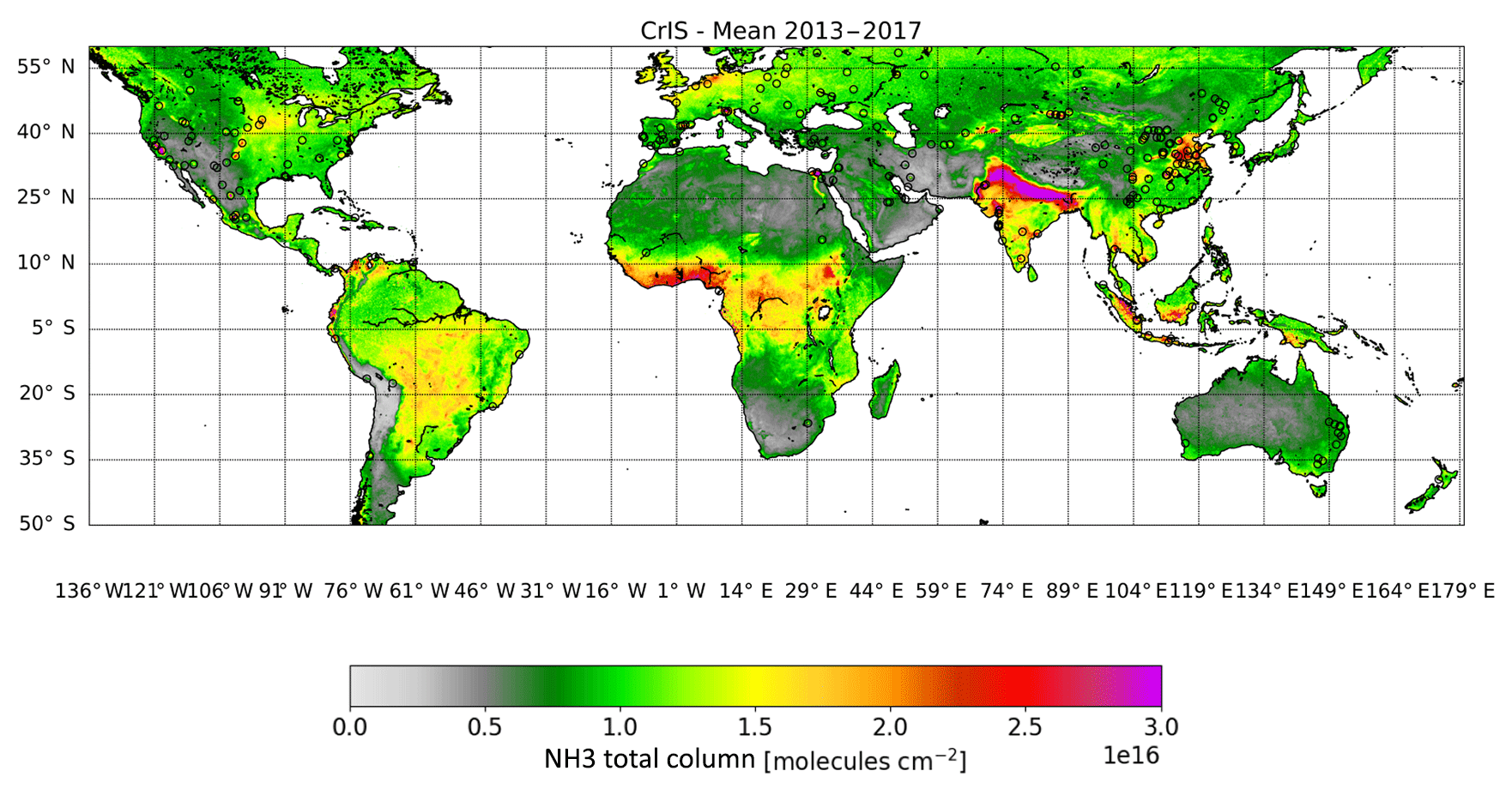
https://www.atmos-chem-phys.net/19/12261/2019/acp-19-12261-2019-f01

Figure 1CrIS NH₃ 5-year mean (2013–2017) total column (molecules cm⁻²) distribution at 0.05^∘ × 0.05^∘ (long, lat) resolution, with the source locations of successful estimates shown by black circles centered around the source locations.

2.1.2 IASI

The IASI instruments aboard the MetOp-A and -B satellites are also in Sun-synchronous orbits and pass locations twice daily with Equator crossing times at 09:30 and 21:30 LST with a difference of about 45 min (Clerbaux et al., 2009). Both IASI instruments have an observational swath width of over 2000 km and have a pixel footprint of around 12 km diameter at nadir viewing angles. The footprints are larger towards the edges of the swaths, with the outermost pixels having a footprint of 20 × 39 km². The Artificial Neural Network for IASI (ANNI) NH₃ v2.2 retrieval product (here called IASI-NNv2.2, unless otherwise noted) (Van Damme et al., 2017) was released in mid-2018. This product is the most recent iteration of the IASI-NH₃ products and an improvement over the previous datasets (Van Damme et al., 2014 a; Whitburn et al., 2016 a). The IASI-NNv2.2 product uses a neural network to link the hyperspectral range index (HRI) with a set of parameters, representing the atmospheric state, to derive the total columns NH₃. The near-real-time IASI-NN data products have small discontinuities in the dataset following updates on the meteorological parameters provided by EUMETSAT. The IASI-NNv2.2 product improved this by providing a reanalysis dataset (ANNI-NH₃-v2.2R-I, here called IASI-NNv2.2(R)) that allows us here to evaluate the emission estimates from year to year. Unless otherwise noted, we use the reanalysis dataset, which is available until the end of 2016. For 2017, we rely on the near-real-time dataset. As of yet, there is no validation study focused specifically on the newest data product. However, the previous data products of IASI have been validated by Dammers et al. (2016, 2017 b) and were found to have a low bias of around 35 % for the older IASI-LUT product (Van Damme et al., 2014 a) depending on the local concentrations, with better performance for regions with high concentrations. The IASI-NNv1.0 product (Whitburn et al., 2016 a) showed better performance, reducing the underestimation to ∼ 25 %–40 % depending on the concentration range. The IASI instrument has a NH₃ detection limit of around 2.4 ppb, as reported by Van Damme et al. (2014 a); assuming that 1 ppb is equal to a total column of $2 \pm 1 \times 10^{15}$ molecules cm⁻², we find a detection limit of $4.8 \pm 2.4 \times 10^{15}$ . In this study, we use the Fast Optimal Retrievals on Layers for IASI (FORLI-CO) product (Hurtmans et al., 2012) to detect and remove the influence of overpassing biomass burning plumes in the region surrounding the emission sources of interest. The IASI-CO product has been validated with Measurement of Ozone on Airbus In-Service Aircraft – In-Service Aircraft for a Global Observing System (MOZAIC-IAGOS) aircraft observations and intercompared with Measurement of Pollution in the Troposphere (MOPITT) observations by George et al. (2015) with the results showing overall good performance. In this study, only daytime IASI-A observations between January 2008 and December 2017 are used, and only daytime observations between March 2013 and December 2017 are used for IASI-B. The NH₃ and CO products are matched on a per observation basis (using the time stamp and the longitude and latitude of the observations) and filtered for conditions with cloud cover over 25 %. A 5-year mean (2013–2017) of IASI-A total column concentrations can be found in Appendix A, Fig. A1.

2.2 NH₃ emission inventories and source locations

A list of potentially observable emission sources was created through a combination of an analysis of global yearly averaged concentration fields and emission inventories. Inspection of the concentration fields revealed that a large number of these locations correlated with known industrial locations. Van Damme et al. (2014 b) showed that there are discrepancies between modeled NH₃ and IASI NH₃ observations for a few of these locations. Fertilizer production and gasification plants were common in this initial search; therefore, we compiled a list of worldwide plant locations based on internet sources (https://globalsyngas.org/resources/world-gasification-database/, last access: 6 December 2018) and used Google Earth to determine the exact locations. To this initial set, we added locations from commonly used and readily available point-source emission inventories. For Europe, the European Pollutant Release and Transfer Register (E-PRTR; http://prtr.ec.europa.eu/, last access: 30 May 2018) is used; for Australia, the National Pollutant Inventory (NPI; http://www.npi.gov.au/, last access: 11 February 2019); for Canada, the National Pollutant Release Inventory (NPRI; https://www.canada.ca/en/services/environment/pollution-waste-management/national-pollutant-release-inventory.html, last access: 11 February 2019); and for the United States, the National Emissions Inventory (NEI; https://www.epa.gov/air-emissions-inventories/national-emissions-inventory-nei, last access: 23 July 2018). From the point-source databases, any locations with NH₃ emissions over 0.3 kt yr⁻¹ were selected. While this would be of an order lower than the expected lower limit of what IASI and CrIS can detect (see Table 2 in Sect. 2.5.2), many of the point-source emissions are not measured but rather based on engineering estimates that can have errors of an order of magnitude (Kuenen et al., 2014; Van Damme et al., 2018). Finally, any locations from the set reported by Van Damme et al. (2018) that were missing from our set have been appended to the final location list.

For a complete list of final locations, see the Supplement. The method used in this study requires a point-source-like emission source. Therefore, the focus of this study is on emission sources that behave as a point source and not regionally sized agricultural emissions or large regions with a considerable number of point sources near one another. Emission estimates will still be attempted for sources that fail to meet the criteria, such as a large number of locations in, for example, the Netherlands, China and India, where extended regions with high NH₃ concentrations exist. Several locations found in the point-source emission databases are within 15 km of one another. In such instances, the locations are merged under a single location name with the location representing multiple sources.

The satellite emission estimates will also be compared to the commonly used Hemispheric Transport Atmospheric Pollution version 2 emission inventory (HTAPv2; http://edgar.jrc.ec.europa.eu/htap_v2/, last access: 10 December 2017; Janssens-Maenhout et al., 2015) and the individual point-source emission databases where available (e.g., the 2014 NPRI, NEI, E-PRTR and the NPI inventories). The HTAPv2 database covers the year 2010 and provides emissions with a high spatial resolution of 0.1^∘ × 0.1^∘. The database consists of a combination of gridded regional emission inventories such as the Model Inter-Comparison Study (MICS) for Asia, Environmental Protection Agency (EPA) for the US and Canada, and the Netherlands Organisation for Applied Scientific Research – Monitoring Atmospheric Composition and Climate (TNO-MACC) II database for Europe. These high-spatial-resolution inventories were complemented by the Emissions Database for Global Atmospheric Research (EDGAR) v4.3 (Crippa et al., 2016) to gap fill missing emissions for countries not covered by the high-resolution databases.

2.3 Meteorology

In this study, a wind rotation approach is used (Pommier et al., 2013; Fioletov et al., 2015; Clarisse et al., 2019), which requires the wind fields for each satellite observation, in order to align the observations in an upwind–downwind coordinate system and thus map out the emission plume. Here, we use the wind fields (U,V) from the European Centre for Medium-Range Weather Forecasts (ECMWF) ERA-Interim dataset (https://apps.ecmwf.int/datasets/data/interim-full-daily/levtype=sfc/, last access: February 2018; Dee et al., 2011) at a resolution of 0.75^∘ × 0.75^∘ (∼ 60 × 80 km² at 45^∘ N) with a 6 h temporal resolution. Most of the observed NH₃ is located in the lower boundary layer (Dammers et al., 2017 a; Y. Zhang et al., 2018; Tevlin et al., 2017). To represent the transport of NH₃ as well as possible, we choose to use an average of the wind fields for the first kilometer of the lower troposphere (∼ 1000–900 hPa). We use the 1000–900 hPa layers for locations at sea level altitude. For locations at higher altitudes, we select layers that cover pressures from the surface pressure up to 100 hPa less above the surface (for example, 800–700 hPa, for a location with a surface pressure of 800 hPa). The first kilometer represents the intermediate case between the potentially lower boundary layers in the morning (IASI overpass, 09:30 LST) and the higher boundary layer heights in the late afternoon (CrIS overpass, 13:30 LST). The wind fields are then interpolated to the position of each individual observation in both space and time. The higher-resolution ERA5 (Copernicus Climate Change Service (C3S), 2017) U,V fields were also tested for this application; however, we found highly variable winds near terrain features, such as hills and coastlines, that were therefore not representative of larger-scale transport.

2.4 Data criteria

The satellite observations measure in the infrared portion of the radiation source, which is emitted from the Earth. Thus, under colder conditions, the thermal signal is decreased, while the instrument noise remains the same, which reduces the overall signal-to-noise ratio (SNR) and sensitivity. Therefore, in this study, we used only observations during warmer conditions between 1 April and 30 September in order to optimize conditions to which the satellites are more sensitive for the Northern Hemisphere. Similarly, only observations made between 1 October and 31 March are used for the Southern Hemisphere. Besides the individual satellite product quality filters, we also correct for the influence of local events with anomalous concentrations, such as manure spreading and fire emissions, by applying a combination of two standard deviation filters. For each of the individual NH₃ emission sources, a subregion is defined that spans 4^∘ × 6^∘ using the complete 10-year dataset of the IASI-A instrument. Each set is then analyzed for NH₃ and CO anomalies, defined as the mean of all observations ±5 and ±3 standard deviations. The corresponding days with unusual NH₃ and CO concentrations and ±1 d are filtered from the dataset. Figure 2 shows an example of the data selection for the location of Togliatti in Russia. The total column time series clearly shows the anomalously high total column concentrations during the Russian fires in 2010 (R'Honi et al., 2013), which are omitted from our dataset using the previously explained steps. Finally, the list of omitted days found in for IASI-A is used to filter the same observation days from both the IASI-B and CrIS datasets to create consistency between the datasets. Note that there is currently no global CrIS-CO dataset available to independently apply the same steps to CrIS-NH₃.

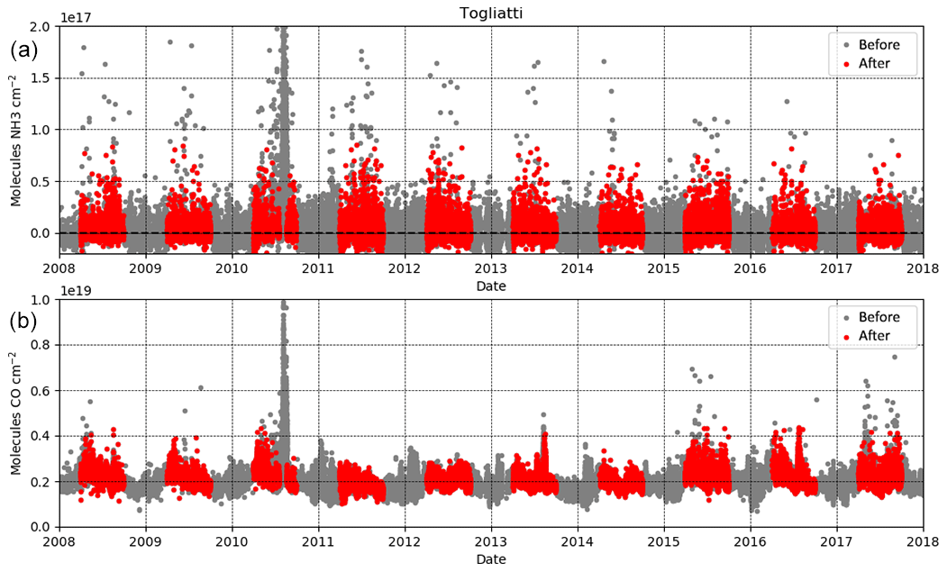
https://www.atmos-chem-phys.net/19/12261/2019/acp-19-12261-2019-f02

Figure 2Data selection example for Togliatti, Russia. Panel (a) shows the IASI-A NH₃ dataset “before” observations are filtered out (grey) and the observations kept “after” (red) the selection. Panel (b) shows the corresponding IASI-A CO observations.

Download

2.5 Method and uncertainties

2.5.1 Wind rotation and fitting algorithm

Previous NH₃ emission studies used a simple mass balance in a predefined box with a specified lifetime (Jacob, 1999; Van Damme et al., 2018; Hickman et al., 2018). Several other methods have been utilized in the past to retrieve emissions of other molecules from satellite observations (Fioletov et al., 2015, 2011; Beirle et al., 2014; de Foy et al., 2015), adding more complexity over time (such as wind rotation) to account for basic advection and diffusion. Here, we follow the wind rotation approach and apply the exponentially modified Gaussian (EMG) method to estimate the lifetime ( $τ = 1 / λ$ , with λ the decay rate), the plume spread (σ) and the emission of the point source. The EMG method (see Appendix B for a detailed EMG description) has been shown to be accurate by de Foy et al. (2014) and has previously been used to estimate SO₂ emissions (Fioletov et al., 2015). It should be noted that, while accurate, the method is sensitive to wind direction and wind speed uncertainties and works best for locations with unobstructed homogeneous terrain. It tends to (underestimate) overestimate lifetime in cases of plume rotation by (overestimating) underestimating wind speeds, with a compensating (decrease) increase in the fitted width parameter. Therefore, we added the altitude and altitude standard deviation above 300 m for the surrounding 1^∘ × 1^∘ to the location list in the Supplement. For the altitude information, we used the GLOBE product (https://www.ngdc.noaa.gov/mgg/topo/globe.html, last access: 16 January 2014; Hastings and Dunbar, 1999). Keep in mind that for some of these locations it is still possible to perform an estimate; however, the results may be less reliable. Observations with wind speeds below 0.5 and above 44.5 km h⁻¹ are filtered from the set to remove abnormally high concentrations during stagnant and low concentration in highly disturbed conditions. To improve SNR, individual CrIS and IASI observations are binned in space (3 km × 4.5 km; crosswind, downwind) and by wind speed (in steps of 2 km h⁻¹ ranging from 0.5 to 44.5 km h⁻¹). For each grid cell, we take all observations within a radius of 15 km around the center of the grid cell, with each observation weighted by a Gaussian weighting function that takes into account the distance from the observation to the grid cell center. We can then fit an EMG function describing the concentrations near the source to the newly found distribution.

https://www.atmos-chem-phys.net/19/12261/2019/acp-19-12261-2019-f03

Figure 3Fit example for the fertilizer plants in the ZMU fertilizer plant in Kirovo-Chepetsk, Russia. Panel (a) shows the original CrIS NH₃ total columns (2013–2017) gridded at a 0.05^∘ × 0.04^∘ (long, lat) resolution and smoothed using the pixel-averaging technique with a 15 km radius to represent the footprint. Panel (b) shows the same observations after applying the wind rotation algorithm and gridding the observations to a 3 km × 4.5 km grid. Panel (d) shows the fit to the observations and (c) the reconstruction of the initial plot using the parameters found in the fit. The cyan dot indicates the source location.

Download

An example demonstrating the procedure and resulting computed emissions for the ZMU fertilizer plant in Kirovo-Chepetsk, Russia, is shown in Figs. 3 and 4, using CrIS 2013–2017 data. The weighted means of the original dataset and rotated dataset are shown in Fig. 3a and b, respectively. The fitted datasets in the longitude–latitude domain and in the downwind–crosswind domain are shown in Fig. 3c and d, with the location of the Kirovo-Chepetsk point source highlighted as a cyan dot. The dashed black box prescribes the area used to fit the plume. This is an example of a weaker source with a well-known source location for which the rotation still shows a roughly defined plume shape. Figure 4a shows the corresponding mean cross section of the binned observations in the downwind direction. Each of the lines corresponds to the mean of a different wind speed interval. It shows that the peak of the plume moves downwind and decreases in amplitude with increased wind speeds as expected. Equation (B1) is fitted to the cells that fall within the striped black square and we find a lifetime of ( $1 / λ) = 3.43$ h, a σ of 10.03 km, a background of 9.85×10¹⁵ molecules cm⁻² and total emissions of 8.93 kt yr⁻¹. The uncertainty shown in the figure only includes the uncertainty of the fit. More on the uncertainty of this method can be found in Sect. 2.5.2. Figure 4b shows the corresponding fit at different wind speeds, with a relatively good fit to the initial distribution. The retrieved parameters can be used to reconstruct the plume shape and initial distribution (Fig. 3c and d). As the background parameter is a single value, the reconstruction will be missing some of the smaller concentration peaks surrounding the source location seen in the top left and right plots.

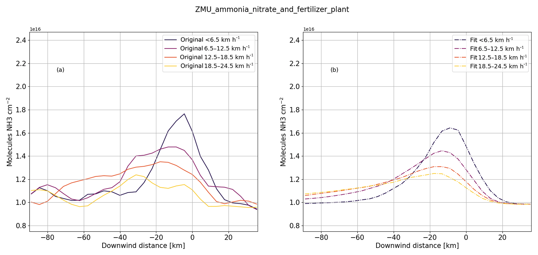
https://www.atmos-chem-phys.net/19/12261/2019/acp-19-12261-2019-f04

Figure 4Mean total column cross sections of the original and reconstructed plume shape for the ZMU fertilizer plant in Kirovo-Chepetsk, Russia. Panel (a) shows the original CrIS NH₃ total column distribution (2013–2017) as a function of wind speed. The cross section is a cross-sectional average of the striped black square shown in Fig. 3. Panel (b) shows the mean cross section of the reconstructed plume.

Download

2.5.2 Method uncertainty and detection limit

In order to estimate the total uncertainty, we describe and add together (in quadrature) the individual sources of error and uncertainty, as listed in Table 1.

Satellite total columns

The dominant cause of uncertainty is the uncertainty in the total column of the satellite product itself. The emission estimates are directly related to the total mass observed by the satellite, and therefore the uncertainty in the total columns can be directly added to the total. Random errors would average out from the large number of observations used in the fit; however, the systematic biases do not. Dammers et al. (2017 b) found a 25 %–40 % negative bias for IASI compared to FTIR observations depending on the total column concentration. Here, we will assume the lower limit of 25 %, as most of the enhancements analyzed in this study have mean total column densities corresponding to the lower range of the bias. Another reason to assume the lower range is that the IASI product used here is an update over the product used in the validation, with much improved performance (Van Damme et al., 2017, Figs. 1, 2, 3). The CrIS-NH₃ observations have a small bias with respect to in situ data (Dammers et al., 2017 b) on the order of 0 %–5 %; however, to account for retrieval errors, we use an uncertainty of 16.5 % following the recent emission study by Adams et al. (2019).

Diurnal and seasonal emission cycles

The observations used here are only representative of the emissions during and before the overpass. A strong diurnal cycle in the emissions is a potential cause of uncertainty. Van Damme et al. (2018) used a model run to estimate the offset between the daily mean total column and the overpass time of IASI-A and found an uncertainty of 4.0±8.0 %. Using simulations for 2014 for the same model, we calculated an uncertainty of 6.3±7.1 % for the IASI-A overpass time and 8.0±10.5 % for the CrIS overpass, with the difference following from the selection of only land-based grid cells and a different simulation year (2014 vs. 2011). The model used in their study attributes a single diurnal emission cycle to all species emitted by the industrial sources emission class. However, for most industrial sources of NH₃, it is highly uncertain what the actual emission cycle is, as in most cases it has not been measured. As for agricultural emissions, the hourly emissions can vary strongly with temperature and soil conditions (Sommer et al., 1991). Furthermore, the emissions will vary a great deal by month, depending again on the temperature and the season in which manure and/or artificial fertilizer is spread over crop and grasslands. As our estimates are only based on satellite measurements done within most of the growing season (Northern Hemisphere), the agricultural estimates can potentially be biased high by 50 % if all emissions take place between 1 April and 30 September. Furthermore, our method weighs towards the months with more observations. Van Damme et al. (2018) found that IASI will get emission estimates that are 4±7 % lower when first binning to monthly averaged grids.

Fitting algorithm

The fitting algorithm is another cause of uncertainty. In this study, we first will do free fits, which include a fit of the lifetime and σ, as well as the emitted amounts and the background (Sect. 3.1). Secondly, using a mean lifetime and σ, calculated from the results of the free fits, we will recalculate the estimates with fixed fits, where the lifetime and the σ are fixed (Sect. 3.2). The uncertainty of the fits is dependent on the amount of information available and the quality of the total column field: in this free-fit case (Fig. 5), we find a mean fitting uncertainty (standard deviation of the fit) of 6.7 %–8.6 %, with the lower range for the IASI instruments. For the fit with fixed parameters, we find a reduced uncertainty of 3.1 %–4.1 %, with the lower range for the IASI instruments. However, any deviations due to the fixed σ and lifetime parameters need to be considered. To calculate the effect, we perturb the parameters by adding a random value taken from a Gaussian random distribution, with a standard deviation found in Table 3, and estimate the emissions. For both the lifetime and σ value (while keeping the other parameter constant), this process is repeated a thousand times for three different locations representing a range of emission enhancements (Donaldsonville, USA; Lethbridge, Canada; and Togliatti, Russia). Taking the standard deviation of the set of estimated emissions for each location and dividing it over the mean, we find a calculated uncertainty for the lifetime and σ of ±29.0 % and ±40.4 % for CrIS and ±40.1 % and ±39.2 % for IASI.

Meteorology

Finally, the uncertainty in the meteorology has a direct effect on our error estimates through Eq. (B3). Assuming an uncertainty of ±1 m s⁻¹ in the wind fields, we calculate the uncertainty by using a similar method as for the lifetime and σ. A random value, taken from a Gaussian random distribution with a standard deviation of ±1 m s⁻¹, is added to both the U and V wind field parameters that were matched to each satellite observation in the set. The emission is then estimated using the perturbed wind fields and a fixed lifetime and σ parameters of 2.5 h and 15 km. This process is then again repeated a thousand times for the three different locations (Donaldsonville, USA; Lethbridge, Canada; and Togliatti, Russia). Taking the standard deviation of the estimated emissions for each location and dividing it over the mean, we find a calculated uncertainty of 2.6 % for IASI and 3.1 % for CrIS.

Table 1Summary of factors of uncertainty in the final satellite emission estimates for IASI-A, -B and CrIS.

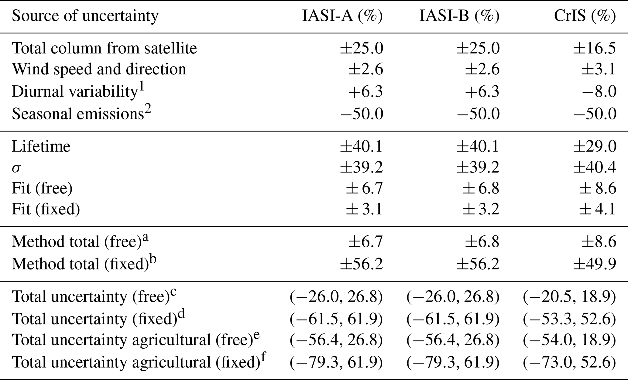
¹ Diurnal cycle via modeling estimate does not include potential effect of biases in diurnal emission profiles. ² For agricultural areas, most emissions are in the spring and summer; hence, these are influenced by the fact that our estimate is for those months only. ^a Sum of the uncertainties from fit (free). ^b Sum of the uncertainties from fit (fixed), lifetime and σ. ^c Sum of the uncertainties from method (free), total column, wind speed and diurnal variability. ^d Sum of the uncertainties from method (fixed), total column, wind speed and diurnal variability. ^e Sum of the uncertainties from method (free), total column, wind speed, diurnal variability and seasonality. ^f Sum of the uncertainties from method (fixed), total column, wind speed, diurnal variability and seasonality.

Download Print Version | Download XLSX

Detection limit

The EMG approach can be used to estimate the emissions for a large range of sources but is limited by a lower detection limit that is directly related to the instrumental detection limit of the satellites. Using Eq. (B1), the limit can be directly estimated over a range of conditions and summarized in Table 2 for the IASI and CrIS instruments. The CrIS instrument has a detector with about 4 times lower spectral noise than IASI, which results in the lower limit of 0.9 ppb under high thermal contrast (TC) atmospheric conditions reported by Shephard and Cady-Pereira (2015) compared to the limit of 2.4 ppb under high TC conditions reported by Van Damme et al. (2014 a). Kharol et al. (2018) reports that CrIS is capable of measuring concentrations down to even 0.2–0.3 ppb under very favorable conditions, but here a more conservative limit of 0.9 ppb is assumed to cover most of the conditions found in the observations. Assuming that 1 ppb is equal to a total column $2 \pm 1 \times 10^{15}$ molecules cm⁻², we find lower limits of $4.8 \pm 2.4 \times 10^{15}$ molecules cm⁻² for IASI and $1.8 \pm 0.9 \times 10^{15}$ molecules cm⁻² for CrIS. The ratio between surface concentration (ppb) and total column density is highly variable and dependent on the shape of the atmospheric profile; therefore, we add a ±50 % range. Furthermore, a σ and lifetime of 15 km and 2.5 h, respectively, and three average wind speeds of 5, 10 and 20 km h⁻¹ are assumed, which are representative values of most of the sources as shown in Sect. 3. The lowest emission detection limits are naturally found for the lowest mean wind speeds, with a detection limit of 9.5±4.7 kt yr⁻¹ for IASI and 3.5±1.8 kt yr⁻¹ for CrIS. These estimates are a conservative lower limit, as plume shapes are not as well defined, making emission estimates less precise. The limits for the 10 and 20 km h⁻¹ cases should be considered as more representative of conditions commonly occurring at most locations.

Van Damme et al. (2014 a)Shephard and Cady-Pereira (2015)

Table 2Estimated emission detection limit.

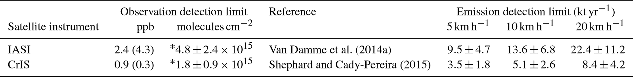
^* Assuming a conversion of 1 ppb $\sim 2 \pm 1 \times 10^{15}$ molecules cm⁻².

Download Print Version | Download XLSX

3 Results

3.1 Lifetime and emission fits

The emission algorithm is applied to each of the source locations obtained as described in Sect. 2.2 and listed in the Supplement for the 5-year interval (2013–2017) of IASI-B and CrIS and the 5- and 10-year (2013 and 2008–2018) intervals of IASI-A data. For quality assurance of the estimated emissions, we filter out low-quality fits with r<0.5 and an upwind–downwind SNR < 2. (McLinden et al., 2016), defined as

\begin{matrix} (1) & SNR = \frac{\overline{C_{d}} - \overline{C_{u}}}{\frac{σ_{d}}{\sqrt{N_{d}}} + \frac{σ_{u}}{\sqrt{N_{u}}}}, \end{matrix}

where $\overline{C_{d}}$ and $\overline{C_{u}}$ are the mean down- and upwind total columns, σ_d and σ_u are the standard deviations, and N_d and N_u are the number of down- and upwind values. Here, we use the SNR filter to remove locations with small enhancements and high regional backgrounds to provide results from single sources with large and sharply defined enhancements (McLinden et al., 2016). Furthermore, fits with lifetimes below 1 h and above 7 h, and σ below 5 km and above 30 km, were filtered out as well. All four values represent the edges of their respective distributions and any value past these edges resulted in bad fits.

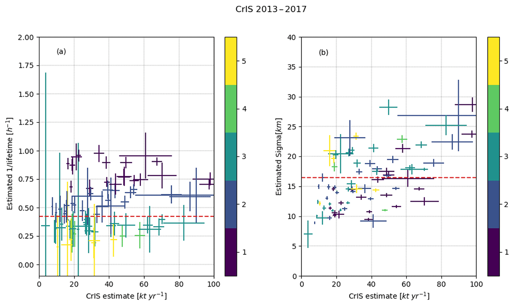
https://www.atmos-chem-phys.net/19/12261/2019/acp-19-12261-2019-f05

Figure 5All successful fits for the 5-year (2013–2017) CrIS dataset with a correlation > 0.5 and a SNR > 2. The left plot (a) shows the fitted emissions vs. the λ parameter and the right plot (b) the fitted emissions vs. the fitted σ with the horizontal and vertical error bars showing the uncertainties of the fit. The color of the bars indicates the fitted lifetime (in hours) rounded to the nearest integer. The horizontal striped red lines show the average of the 1∕λ and σ parameters.

Download

Figure 5 shows the results for all successful fits for CrIS data over the 5-year (2013–2017) interval. The resulting set has a mean lifetime of 2.35±1.16 h and a mean σ of 16.42±5.13 km.

Table 3Mean lifetime and σ for all successful fits with a correlation > 0.5 and a SNR > 2 for the 5-year IASI-A, IASI-B and CrIS and 10-year IASI-A datasets.

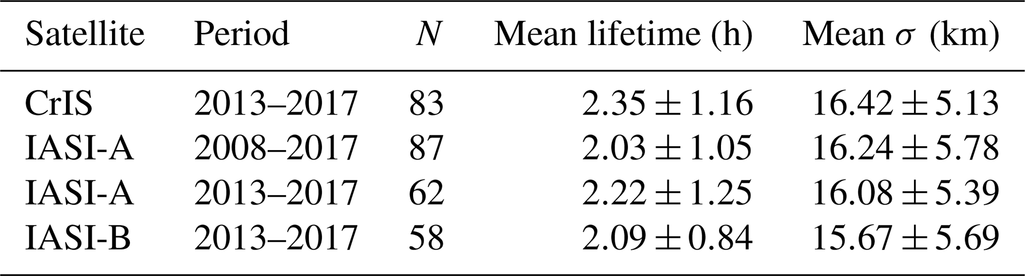
Download Print Version | Download XLSX

Table 3 and Figs. C1, C2 and C3 in Appendix C show the corresponding results for IASI-B and the 5- and 10-year interval IASI-A sets; all show similar results, which might be expected for effective σ given the similar footprint sizes of the instruments. For all sets, we find a lifetime between 2.03 and 2.32 h with a standard deviation ∼1 h. This is shorter than most of the measured and modeled estimates reported in literature, ranging from a few hours up to 2 d. Most of the longer lifetimes were determined by analyzing short- and long-range transport of fire plumes, emitted near the surface or injected at higher altitudes (Yokelson et al., 2009; R'Honi et al., 2013; Whitburn et al., 2015; Lutsch et al., 2016; Adams et al., 2019), which are of limited applicability here, as the high concentrations of other species found in a plume that gets injected into the free troposphere are not very comparable to normal surface conditions. The only other study reporting satellite estimates of NH₃ for agricultural and industrial sources, Van Damme et al. (2018), used a lifetime of 12 h, quoting the limited data available in literature. Van Damme et al. (2018) also calculated emissions for lifetimes of 1 and 48 h as upper and lower estimates which will be of more use for later discussion. Nonetheless, the decay of the NH₃ plume over a distance ∼80 km, as seen in Fig. 4 (which is typical), suggests an effective lifetime on the order of 2–4 h. The mean σ of ∼15 km is in line with earlier estimates for SO₂ (Fioletov et al., 2015), with the σ mostly varying with spatial extent of the source, differences in diffusion for each location and the influence of nearby sources. The slightly larger value for CrIS is consistent with its slightly coarser spatial resolution. The wide distribution around the mean can potentially also follow from underconstrained fits as well as the large spatial extent of some of emission sources. As seen in Fig. 5b (and Figs. C1, C2 and C3 in Appendix C), the σ parameter shows a positive relation with the total estimated emission. The largest emission estimates are for agricultural hotspots, which in some cases are poorly described as single point sources and any result for such examples should be treated with caution.

3.2 Constrained fits and comparison

As indicated by the limited number of points shown in Fig. 5 (and Figs. C1, C2 and C3 in Appendix C), only a few locations have plume shapes with large enough total column enhancements for estimating the lifetime 1∕λ, the spread σ, background B and emissions a, which require a non-linear, and hence less stable, fit. To increase the number of converging fits, the lifetime and σ parameters are fixed to 2.5 h and 15 km, similar to the weighted means found in Table 3, thus requiring only a linear fit. The algorithm was then reapplied to all locations in order to determine emission estimates for those with weaker enhancements in which the original fits failed due to a lack of independent information to fit these additional parameters. The results of those fits are quality controlled as before (see Sect. 3.1) but now with a weaker correlation filter (r<0.30) to adjust for the stricter fit parameters. All results, including the correlations, are merged into the location list and can be found in the Supplement.

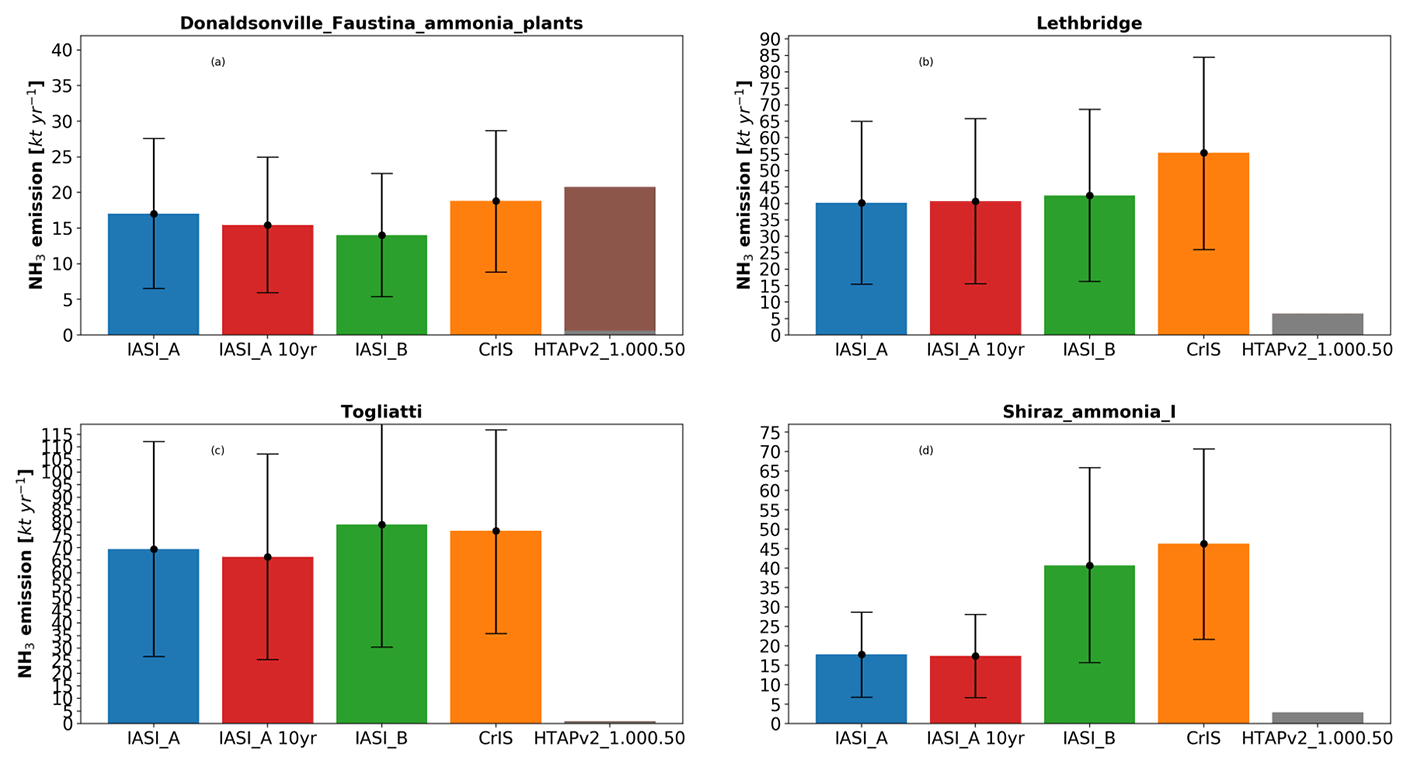
https://www.atmos-chem-phys.net/19/12261/2019/acp-19-12261-2019-f06

Figure 6Comparison of the IASI-A (5 years, blue; 10 years, red), IASI-B (green) and CrIS (orange) emission estimated using fixed parameters for lifetime and σ, and the corresponding total emission found in the HTAPv2 inventory for a square 1.00^∘ × 0.50^∘ (long, lat) surrounding the location. The grey part of the bar indicates the agricultural emission total, while the brown section represents all other sources.

Download

Figure 6 demonstrates a few examples of emissions from the fit results compared to the emissions calculated from the HTAPv2 emission inventory and integrated over 1.00^∘ × 0.50^∘. Figure 6a shows results for the NH₃ production plants in Donaldsonville and Faustina in the United States, with all four satellite estimates showing comparable results. This is one of the few examples that compares well with the current inventory estimates, as can be seen from the other three examples. Figure 6b shows the results for Lethbridge, Canada, where a large number of concentrated animal feeding operations (CAFOs) can be found. The estimates compare poorly with the estimate calculated from HTAPv2. The difference can be explained by a few factors: first, as only the observations between 1 April and 30 September are used, the estimate is only representative of the spring and summertime emissions. Outside of the spring and summer period, emissions of CAFOs are expected to be lower due to slower volatilization rates (Gyldenkærne et al., 2005); second, differences in agricultural practices, with most fertilizer being spread in early spring (Sheppard et al., 2010), which can occur early or late depending on the year. If most emissions occur during the 6 spring and summer months, we would need to halve the satellite estimates, which would bring the estimates closer. Figure 6c and d show the estimates for the NH₃ plants in Togliatti, Russia, and near Shiraz, Iran, respectively. In three of these four cases, the satellite emission estimates do not agree with the HTAPv2 inventory, with the inventory showing much lower total emissions. Most of the industrial emissions are computed using empirical estimates and are not measured (E-PRTR database); therefore, large differences can be expected. The fits for the NH₃ production plants near Shiraz are a good example of the limited applicability of this method in regions with large elevation changes nearby and only a single outflow direction. While the fits may seem reasonable (see Figs. D1, D2 and D3 in the Appendix), the overall wind speed is very low and the plume shape is not well defined. This limitation is more visible for IASI-A than for IASI-B and CrIS, which can be due to small deviations in the concentration field.

https://www.atmos-chem-phys.net/19/12261/2019/acp-19-12261-2019-f07

Figure 7IASI-A vs. IASI-B and IASI-A vs. CrIS for locations with r>0.5 with a fixed σ of 15 km and lifetime of 2.5 h. 2013–2017. R indicates the correlation between the sets, N the number of locations, S and I the resulting slope and intercept of the regression (RMA) and the mean absolute difference (y−x) and the mean relative difference ( $y - x / (0.5 y + 0.5 x)$ ) (MAD and MRD). Triangles indicate locations with agricultural emissions equal to and above the sum of all other classes in the HTAPv2 inventory.

Download

The emission estimates from the fits with fixed lifetime and spread over the locations with r>0.5 from all three satellites are in good agreement (Fig. 7). IASI-A and -B compare very well with a tight distribution around the x:y line and a few higher estimates for IASI-B biasing the fit high. The positive bias between the IASI instruments and CrIS is consistent with the different overpass times. Compared to the IASI 09:30 LST overpass, the top of the boundary layer will be higher at the CrIS 13:30 LST overpass. Especially during days with low thermal contrast in the morning, IASI might not observe the lowest layer of the troposphere and miss a fraction of the atmospheric columns, leading to an underestimation of the emissions. Emissions from agricultural sources are also expected to be higher in the afternoon because of higher temperatures, which increase volatilization rates. Lastly, while there is a bias between the CrIS and IASI-A and -B total columns, an offset between the products does not have too much of an impact on emissions, as this should be caught by the background parameter. Any ratio between the products, however, can create a ratio in the emission estimates. Dammers et al. (2017 b) validated the CrIS and IASI(-A) NH₃ products. Compared to the FTIR-NH₃ product, the IASI product was biased low for lower total columns, while CrIS biases high. For increasing total column densities, the bias in the CrIS columns disappears, while IASI shows a smaller and smaller negative bias. Coarsely transformed to an IASI-to-CrIS ratio, it can be expected that the CrIS estimates will be higher than IASI, as IASI likely underestimates the total columns and thus the emission total. As noted earlier, the validation by Dammers et al. (2017 b) was for the previous versions of both the CrIS and IASI retrievals. The IASI retrieval has evolved, with the new retrieval showing much improved performance (Van Damme et al., 2017).

https://www.atmos-chem-phys.net/19/12261/2019/acp-19-12261-2019-f08

Figure 8IASI-A, IASI-B and CrIS emission estimates vs. the regional point-source emission inventories. Point-source values are the sum of all emissions in a square 0.50^∘ × 0.25^∘ (long, lat) surrounding each source location.

Download

https://www.atmos-chem-phys.net/19/12261/2019/acp-19-12261-2019-f09

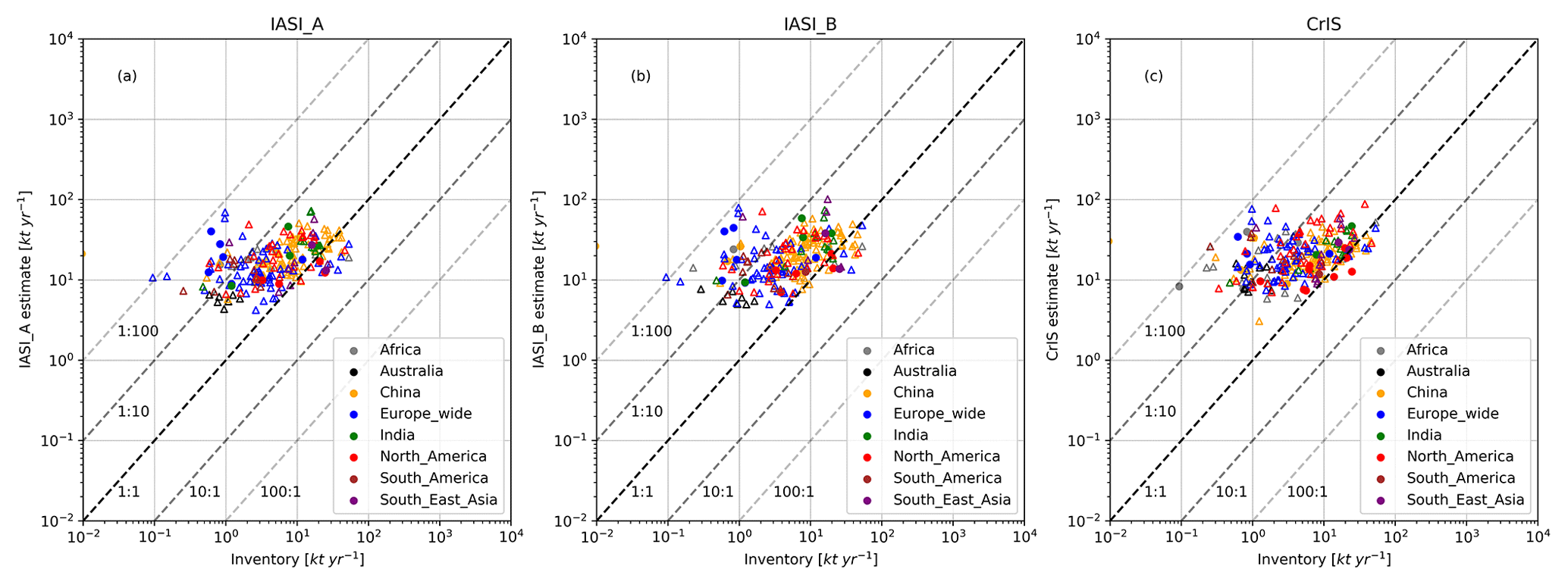
Figure 9HTAPv2 emission database vs. satellite estimates. HTAPv2 emissions are available globally and the sum of all emissions in a square 1.00^∘ × 0.50^∘ (long, lat) surrounding each source location. Open triangles indicate locations with agricultural emissions equal to and above the sum of all other classes in the inventory.

Download

Figure 8 shows a comparison of emissions between (fixed) fits to the satellite data and the point emission databases of the United States (NEI), Canada (NPI), Europe (E-PRTR) and Australia (NPI) for point sources in the emission databases. Overall, the point-source inventories compare poorly to the fitted emissions. Only the E-PRTR inventory has a majority of locations for which the fitted totals are within an order of magnitude of the totals from the inventory. While an uncertainty of 100 %–300 % is to be expected following Kuenen et al. (2014), some estimates are multiple orders larger than reported emissions. The satellite emission fits compare slightly better to the HTAPv2 database (Figs. 9 and 10); here, we summed the satellite emission fits to all HTAPv2 emissions in a 1.00^∘ × 0.50^∘ box surrounding the source location. However, here we also find that in 55 (IASI-A:33, IASI-B:39) cases the inventories emissions are either missing or underestimated by more than an order of magnitude. A total of 72 (IASI-A:71, IASI-B:64) locations are within a factor of 2 of the CrIS emission estimates and in most cases represent agricultural regions (illustrated by the triangles). These results, using a more sophisticated method to estimate the satellite-based emissions, confirm the underestimation of the current emission inventory reported for EDGAR v4.3.1 by Van Damme et al. (2018). A comparison between the results of this study and those obtained using a box model approach is provided in Fig. E1 in Appendix E.

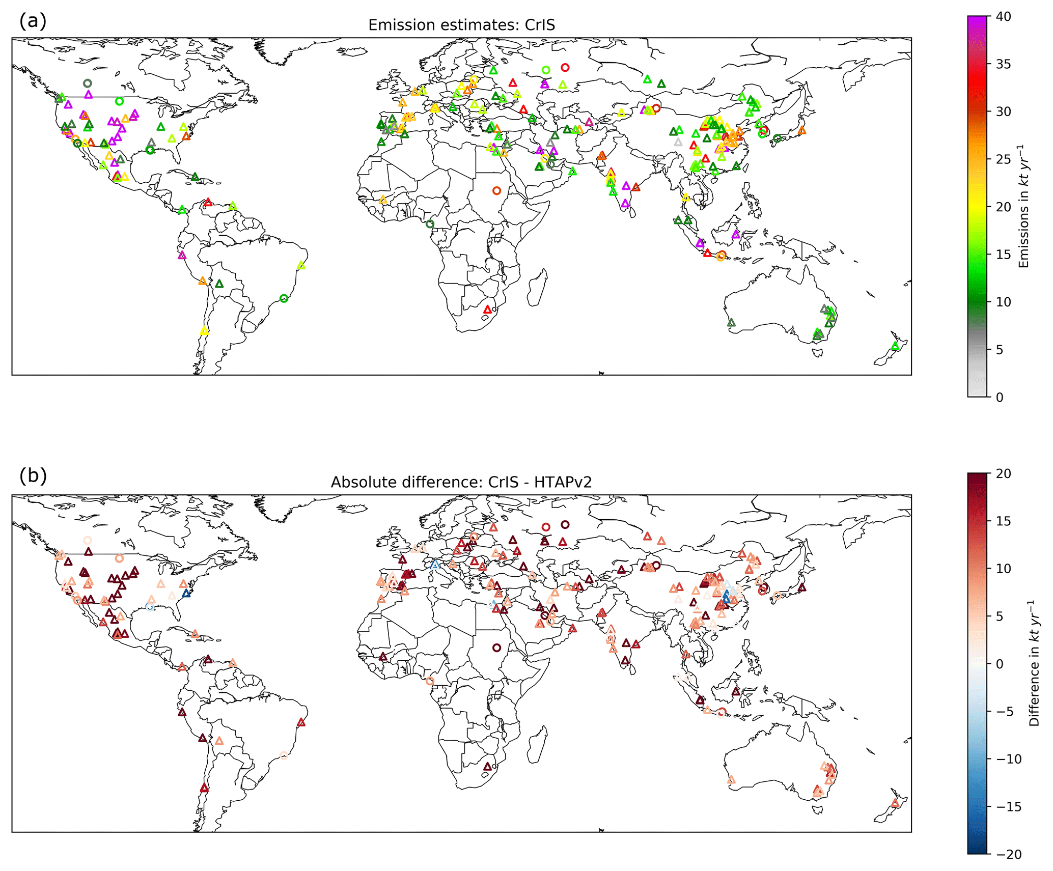
https://www.atmos-chem-phys.net/19/12261/2019/acp-19-12261-2019-f10

Figure 10Global overview of CrIS emission estimates compared to the HTAPv2 inventory for locations with r>0.3, SNR > 2, a fixed σ of 15 km and a lifetime of 2.5 h. Panel (a) shows the CrIS emission estimates and (b) the difference between the CrIS estimates and the corresponding emissions found in the HTAPv2 inventory for a square 1.00^∘ × 0.50^∘ (long, lat) surrounding the locations. Open triangles indicate locations with agricultural emissions equal to and above the sum of all other classes in the inventory.

For the exact dimensions of the individual regions mentioned here, see Table F1 and Fig. F1 in Appendix F. Table 4 shows the total emissions estimated with these studies compared to the total emissions in the HTAPv2 inventory. We find that our method estimates that 3537 kt yr⁻¹ is missing in the inventory for the locations used in this study, which converts to a factor of ∼2.5 between satellite-estimated emissions and the current HTAPv2 emissions. Based upon the total NH₃ emissions in HTAPv2, the locations used in this study account for around 5 % of the total yearly global emissions.

Table 4Summary of the CrIS, IASI-A and IASI-B emission estimates per region vs. HTAPv2 inventory entries for all successful fits with a correlation > 0.3 and a SNR > 2. Each entry represents the CrIS value with the IASI-A and IASI-B values following between the brackets: CrIS (IASI-A, IASI-B).

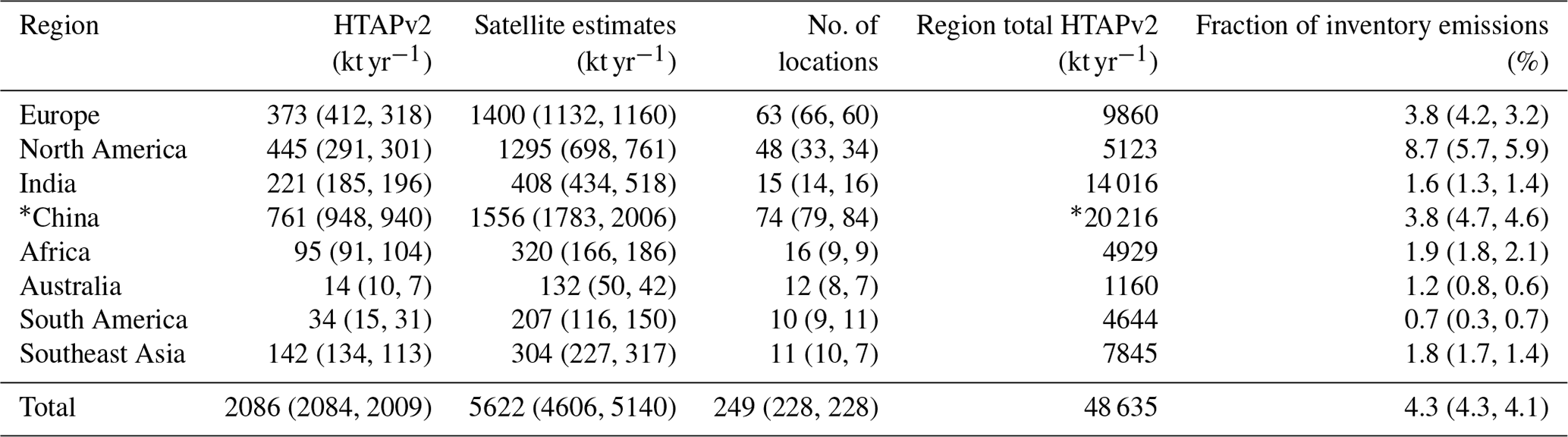
^* The China region includes a large part of northern India; therefore, the emissions may seem higher than expected.

Download Print Version | Download XLSX

3.3 Emission time series

Instead of estimating average emissions over the entire 2008–2017 interval, it is also possible to calculate yearly estimates using a running mean over 3 years of data. Estimates using only a single year of observations were only possible for the strongest sources. Therefore, instead we use a set of 3 years, with the edges of the series consisting of 2 years. By combining a manual search through the results with information on each source location, a number of interesting emission time series were revealed. Figure 11 shows the emission time series for a number of source locations estimated from IASI-A data, which have the longest period of record of the satellite instruments used in this study. Figure 11a shows the emission time series of locations situated in or near conflict zones. Both the Horliwka/Gorlovka and Severodonetsk petrochemical plants are located in the east of Ukraine in or near the front line of the war in the Donbass region. The conflict started around March 2014, which coincides with the rapid decline in emissions from 2013 onward (the 3-year set uses the previous year), following the closure of the fertilizer production plants (Dimitry Firtash, 2014). Another example is the agricultural regions south of Homs and east of Damascus, which have both been impacted by the Syrian civil war. The civil war started around 2011, and the reduced emissions are especially visible for the region south of Homs, which was in the rebel-/opposition-controlled region at the time. Similarly, the agricultural region east of Damascus had reduced emissions for this period, which reflects the state of most agricultural activities throughout Syria during the war (FAO, 2017). Figure 11b shows the examples of the NH₃ factories in Nevinnomyssk, Russia, and Zalantun (Hulunbeir), China, regions, which both show increasing emissions. The increase seen for the NH₃ plant in Nevinnomyssk follows from the increased production as of 2010/2011, after upgrades to the plant between 2008 and 2011 (EuroChem Group, 2008). The Zalantun NH₃ plant was built in 2010 and started production at the end of 2011 (full production at the start of 2012; Fufeng Group, 2012). Figure 11c shows the example of a number of locations where decreasing emissions were found connected to reduced production. The Salavat (Russia) petrochemical complex reduced production to permit upgrades (Gazprom, 2017) and is expected to increase production from 2017 onward. The NH₃ plant in Turnu Măgurele, Romania, decreased production for years before closing down (ICIS, 2011), following cuts to subsidized gas. The same subsidy cuts affected the plant in Bacău, Romania, which was reported by Van Damme et al. (2018). The nickel refinery in Yabulu, Australia, increased production in the early 2010s following new ownership and subsequent investments (Business Review Australia, 2010). However, on several occasions, (potential) tailing pond leaks to the Great Barrier Reef were reported (ABC News/Ben Millington, 2016) and subsequently the refinery has been (temporarily) shut down since 2016 (ABC News, 2016). Finally, there is the case of the NH₃ plant in El Tablazo, Venezuela, where NH₃ emissions have decreased since 2010, which seems to be due to the lack of fuel and mechanical issues since the start of the shortages in Venezuela in 2010 (ChemStrategy, 2018). For comparison with the yearly emission estimates mentioned by Van Damme et al. (2018) (Fig. 4), see Fig. E2 in Appendix E.

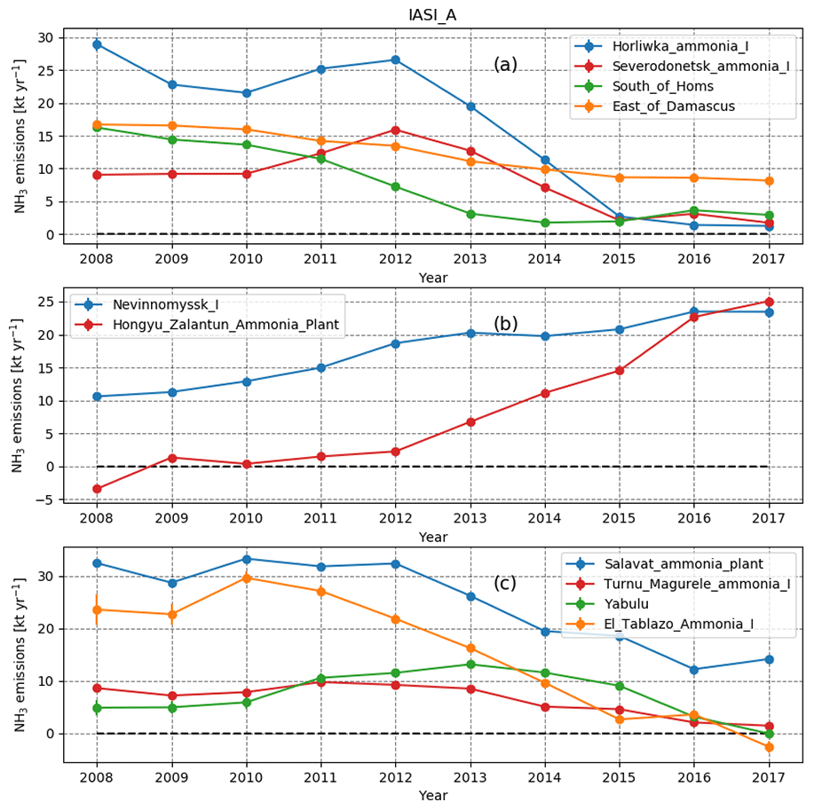
https://www.atmos-chem-phys.net/19/12261/2019/acp-19-12261-2019-f11

Figure 11Annual variations in the IASI-A NH₃ emission estimates for (a) sources in conflict zones, (b) industrial sources that increased production and (c) industrial sources that reduced production.

Download

https://www.atmos-chem-phys.net/19/12261/2019/acp-19-12261-2019-f12

Figure 12Regionally summed annual IASI-A NH₃ emission estimates. The plot in panel (a) shows the total emissions per year for each region, with N the number of sources used for each sum and S the Sen slope estimate of the 10 years of data for all cases with a significant Mann–Kendall trend test. The error bars represent the uncertainty of each of the individual sources added in quadrature. The plot in panel (b) shows the emissions normalized by base year 2010, with N the number of sources used for each sum and S the Sen slope estimate of the 10 years of data for all cases with a significant Mann–Kendall trend test.

Download

Annual emissions over extended regions can also be calculated. Regions are defined in Table F1 in Appendix F. Figure 12 shows the annual emissions estimated from IASI-A in each region and the emissions relative to the HTAPv2 inventories' base year of 2010. Only locations with both successful 5-year IASI-A fits and with successful fits for all the 10 individual years were used. Note that the point sources only constitute around 5 % to 10 % of all emissions in most regions, which in combination with the relatively few points in our set means that at best the increases and decreases should be seen as a tentative estimate of changes in each region and not as a significant trend of all the emissions in region. Figure 12a shows the sum of the annual emissions of the emission sources in each region. Figure 12b shows the same time series but normalized to the emissions of 2010. The year 2010 was chosen as this is the same as the HTAPv2 base year. To each time series, the Mann–Kendall test (Kendall, 1938; Mann, 1945) is applied to calculate if there is a significant trend. In cases with a significant trend, we estimate the slope using Sen's slope estimate (Sen, 1968), which is insensitive to outliers. For three regions, there are significant trends, which are all increasing. The China region (p<0.01) shows the most significant absolute changes, with a change of about 2.6 % yr⁻¹. The multiannual increase mostly follows from an increase in fertilizer production and agricultural emissions. A similar increase is seen in the study by Warner et al. (2017), who attributed it to an increase in fertilizer use in the region. For the European region, we find a very small change of about 0.9 % yr⁻¹ (p<0.05). Finally, the South American region shows the largest relative change, with an increase of about 5.0 % yr⁻¹ (p<0.01). The increase in South America follows mostly from changes in agricultural emissions, which were also reported by Warner et al. (2017) and Van Damme et al. (2018).

4 Summary and conclusions

In this study, we presented the first NH₃ emission estimates based on the CrIS-NH₃ satellite observations, where both the emissions and lifetimes of NH₃ are derived simultaneously for a variety of agricultural and industrial point sources. Results are consistent between the CrIS and IASI satellites, with an average lifetime of 2.4±1.2 h and a σ of 16.4±5.1 km for CrIS, 2.2±1.3 h and 16.1±5.4 km for IASI-A, and 2.1±0.8 and 15.7±5.7 km for IASI-B. Using an average lifetime of 2.5 h and a σ of 15 km, we found comparable emission totals for all three satellites with correlations of r=0.91, r=0.80 and r=0.78 between IASI-A and IASI-B, IASI-A and CrIS, and IASI-B and CrIS, respectively. The CrIS emission estimates are on average higher than the emissions derived from IASI-A and -B observations but are within the uncertainty of the estimates. The differences in the emissions can be due to the bias between the satellite products, as well as the potential influence of the different sampling times of the satellites in combination with the strong diurnal cycles of the emissions. With our method, we found 249 sources with emission levels that are detectable by the CrIS satellite. Comparison with the HTAPv2 inventory shows that there are currently 55 sources missing or underestimated by more than an order of magnitude in the inventory, and only 72 sources have emissions that differ from the HTAPv2 inventory by less than a factor of 2. For IASI-A (and IASI-B), we found similar numbers, with, respectively, 228 (228) total sources detected, with 33 (39) sources missing from the inventory and only 71 (64) sources where the HTAPv2 emissions fall within a factor of 2 of the satellite estimates. All the sources successfully estimated with CrIS combined have a total emission of 5622 kt yr⁻¹, which is about ∼2.5 times more than the current amount in the HTAPv2 inventory (2086 kt yr⁻¹) over the same locations. Applying the same method to the longer 10-year IASI-A dataset for yearly estimates, we are able to observe short- and long-term variations in emissions from both large and small sources, with emissions matching changes to production and other local developments. The temporal variations are consistent with those earlier found by Van Damme et al. (2018). The regional trends in the emissions are similar to earlier findings based on the AIRS satellite (Warner et al., 2017). The results, however, may not necessarily be reflective of the entire region, as only the larger more isolated sources are included in these studies satellite estimates.

The sum of the HTAPv2 emissions from all point sources with successful fits makes up about 5 % of the global total emissions in the HTAPv2 inventory. Future work should focus on reducing the uncertainties and applying similar methods to estimate emissions for regions with a large number of sources in close proximity or with large spatial extent (Fioletov et al., 2017), as well as emissions from fires (Mebust et al., 2011; Adams et al., 2019). The estimates are based on the spring and summertime observations and are representative of those 6 months. The yearly emission total follows from the assumption of constant emission cycle throughout the year, which can lead to an overestimation for sources with a strong seasonal cycle. Seasonal and diurnal emission cycles are currently one of the larger causes of uncertainty in satellite-derived emissions. There is an overall lack of NH₃ emission measurements, with only a few studies reporting flux measurements (Zöll et al., 2016; Schrader et al., 2018). Flux measurements for a larger number of locations and longer periods would be of great value to constrain diurnal emission cycles, which in turn will greatly reduce the uncertainty of satellite-based approaches. The second largest source of uncertainty is the bias in and between the CrIS and IASI products. Both satellite products have seen several improvements and/or upgrades (Van Damme et al., 2017; Shephard et al., 2019) and should be revalidated, both with FTIR-NH₃ (Dammers et al., 2016, 2017 b) and/or ground- and aircraft-based measurements (Van Damme et al., 2015). Furthermore, validation of the nighttime NH₃ observations could enable use of the nighttime observations to constrain nighttime emissions and possibly lifetime of NH₃.

Code and data availability

The near-real-time IASI NH₃ (ANNI-NH₃-v2.1) and CO (FORLI) data used in this study are freely available through the Aeris database http://iasi.aeris-data.fr/nh3/ (last access: 13 June 2018) and http://iasi.aeris-data.fr/CO/ (last access: 17 April 2018). The CrIS data are currently available upon request and will be publicly released at the end of 2019. All Python code used to create any of the figures and/or to create the underlying data is available on request.

Appendix A: IASI-A mean total column map

https://www.atmos-chem-phys.net/19/12261/2019/acp-19-12261-2019-f13

Figure A1IASI-A NH₃ 5-year mean (2013–2017) total column (molecules cm⁻²) distribution at 0.05^∘ × 0.05^∘ (long, lat) resolution, The source locations with successful emission estimates are shown by black circles centered around the source locations.

Appendix B: The EMG fitting function

The function used in this study is a combination of an exponentially modified Gaussian (EMG) g(y,s) and a Gaussian function f(x,y) scaled by factor a as shown in Eq. (B1):

\begin{matrix} (B1) & {Column}_{{NH}_{3}} (x, y, s) = a \cdot f (x, y) \cdot g (y, s) + B \\ (B2) & f (x, y) = \frac{1}{σ_{1} \sqrt{2 π}} \exp (- \frac{x^{2}}{2 σ_{1}^{2}}) \\ (B3) & g (y, s) = \frac{λ_{1}}{2} \exp (\frac{λ_{1} (λ_{1} σ^{2} + 2 y)}{2}) erfc (\frac{λ_{1} σ^{2} + y}{\sqrt{2} σ}) \\ (B4) & σ_{1} = \{\begin{cases} \sqrt{σ^{2} - 1.5 y} & , y < 0 \\ σ & , y \geq 0 \end{cases} \\ (B5) & λ_{1} = \frac{λ}{s}, \end{matrix}

in which x, y describe the crosswind and downwind location of the satellite pixel with respect to the source location (in kilometers), s (in km h⁻¹) the wind speed, σ the parameter describing the width of the Gaussian (in kilometers), λ the decay rate (h⁻¹), B the background total column concentration (molecules cm⁻²), a the emission enhancement (molecules cm⁻²) and $erfc (x) = \frac{2}{\sqrt{π}} \int_{x}^{\infty} e^{- t^{2}} d t$ . Equation (B3), g(y,s), is a convolution of a Gaussian describing the diffusion (with parameter σ the width) that smooths an exponential function, which describes the exponential decay of the selected species in the downwind direction (with lifetime $τ = 1 / λ$ and $t = - y / s$ ; thus, decay is $\sim \exp (λ y / s)$ and $λ_{1} = λ / s$ ; Eq. B5). Equation (B2), f(x,y), describes the diffusion of our species perpendicular to the downwind direction. Similar to Fioletov et al. (2015), we adjusted the shape of the plume downwind to account for the size of the pixel shape and ensure convergence for a larger number of fits. Using a non-linear fitting algorithm, we can fit the equation to the total column distribution and estimate a, σ and λ. The fits are performed in Python using the non-linear curvefit package from the SciPy module (Jones et al., 2001) using the Levenberg–Marquardt algorithm, which minimizes the difference between the given distribution and the fitted values. The fit is performed on a subset of the rotated grid, spanning 25 km in each crosswind direction, and 36 and 90 km in the upwind and downwind directions. For our starting parameters, we use 15 km, 1∕3 h⁻¹, 1×10¹⁹ molecules and 1×10¹⁵ molecules cm⁻² for σ, λ, a and B, respectively, representing an average of the σ parameters found in Fioletov et al. (2015), an initial lifetime estimate of 3 h, the initial enhancement estimate and a low range estimate of the bias found in IASI and CrIS mean distributions. From a combination of a and λ, we then find the emission rate $E = a \cdot λ$ (Fioletov et al., 2015).

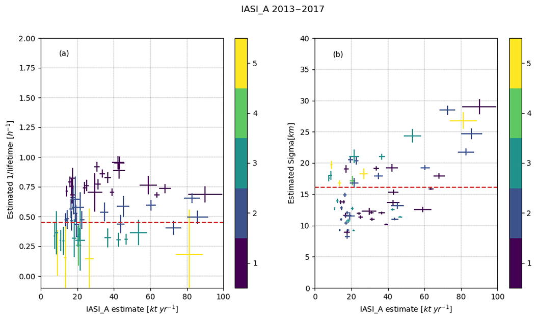
Appendix C: Results for all locations, free σ and lifetime

https://www.atmos-chem-phys.net/19/12261/2019/acp-19-12261-2019-f14

Figure C1All successful fits for the 5-year (2013–2017) IASI-A dataset with a correlation > 0.5 and a SNR > 2. Panel (a) shows the fitted emissions vs. the λ parameter and (b) the fitted emissions vs. the fitted σ with the horizontal and vertical error bars showing the uncertainties of the fit. The color of the bars indicates the fitted lifetime rounded to the nearest integer. The horizontal striped red lines show the weighted average of the λ and σ parameters.

Download

https://www.atmos-chem-phys.net/19/12261/2019/acp-19-12261-2019-f15

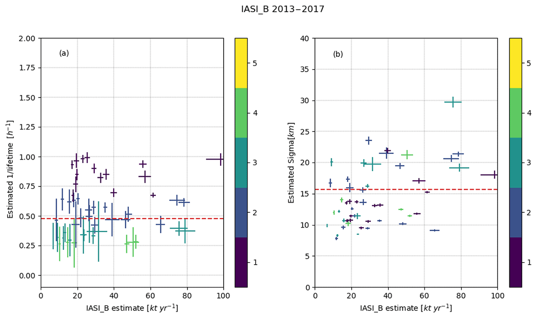
Figure C2All successful fits for the 5-year (2013–2017) IASI-B dataset with a correlation > 0.5 and a SNR > 2. Panel (a) shows the fitted emissions vs. the λ parameter and (b) the fitted emissions vs. the fitted σ with the horizontal and vertical error bars showing the uncertainties of the fit. The color of the bars indicates the fitted lifetime rounded to the nearest integer. The horizontal striped red lines show the weighted average of the λ and σ parameters.

Download

https://www.atmos-chem-phys.net/19/12261/2019/acp-19-12261-2019-f16

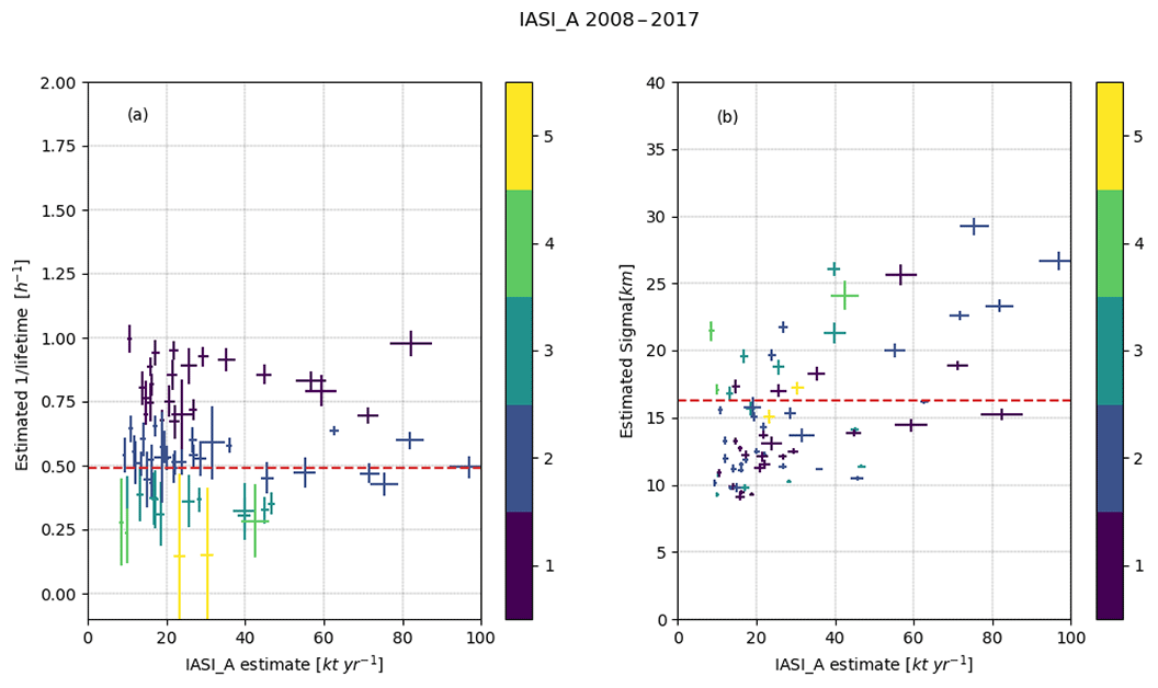
Figure C3All successful fits for the 10-year (2008–2017) IASI-A dataset with a correlation > 0.5 and a SNR > 2. Panel (a) shows the fitted emissions vs. the λ parameter and (b) the fitted emissions vs. the fitted σ with the horizontal and vertical error bars showing the uncertainties of the fit. The color of the bars indicates the fitted lifetime rounded to the nearest integer. The horizontal striped red lines show the weighted average of the λ and σ parameters.

Download

Appendix D: Supporting material: fit results for the NH₃ production plant near Shiraz, Iran

https://www.atmos-chem-phys.net/19/12261/2019/acp-19-12261-2019-f17

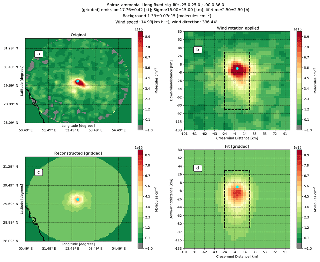
Figure D1Fit example for the fertilizer plants in Shiraz, Iran. Panel (a) shows the original IASI-A NH₃ total columns (2013–2017) gridded at a 0.05^∘ × 0.04^∘ (long, lat) resolution with the pixel-averaging technique with a 15 km radius to represent the footprint. Panel (b) shows the same observations after applying the wind rotation algorithm and gridding the observations to a 3 km × 4.5 km grid. Panel (d) shows the fit to the observations and (c) the reconstruction of the initial plot using the parameters found in the fit.

Download

https://www.atmos-chem-phys.net/19/12261/2019/acp-19-12261-2019-f18

Figure D2Fit example for the fertilizer plants in Shiraz, Iran. Panel (a) shows the original IASI-B NH₃ total columns (2013–2017) gridded at a 0.05^∘ × 0.04^∘ (long, lat) resolution with the pixel-averaging technique with a 15 km radius to represent the footprint. Panel (b) shows the same observations after applying the wind rotation algorithm and gridding the observations to a 3 km × 4.5 km grid. Panel (d) shows the fit to the observations and (c) the reconstruction of the initial plot using the parameters found in the fit.

Download

https://www.atmos-chem-phys.net/19/12261/2019/acp-19-12261-2019-f19

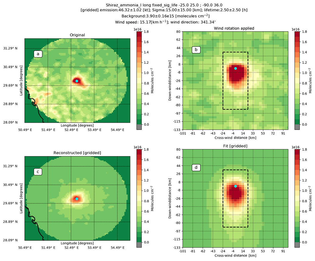
Figure D3Fit example for the fertilizer plants in Shiraz, Iran. Panel (a) shows the original CrIS NH₃ total columns (2013–2017) gridded at a 0.05^∘ × 0.04^∘ (long, lat) resolution with the pixel-averaging technique with a 15 km radius to represent the footprint. Panel (b) shows the same observations after applying the wind rotation algorithm and gridding the observations to a 3 km × 4.5 km grid. Panel (d) shows the fit to the observations and (c) the reconstruction of the initial plot using the parameters found in the fit.

Download

Appendix E: Comparison to Van Damme et al. (2018)

This study's results expand upon earlier work by Van Damme et al. (2018). The method used in this study is more advanced, with the addition of wind rotation and a more complex treatment of the plume shape and transport, which enables the additional estimation of lifetime and plume spread (σ). For well-isolated point sources, the method has been shown to be more sensitive and accurate by McLinden et al. (2016) and de Foy et al. (2014) and has previously been successfully used to more accurately estimate SO₂ emissions (Fioletov et al., 2015). Figure E1 shows the comparison of emission estimates using a box model approach (Van Damme et al., 2018) vs. the results of this study. As Van Damme et al. (2018) used a mean lifetime of 12 for their reported results, we scale the estimates by a factor (12∕2.5) to adjust the lifetime to the lifetime found in this study. In addition, they used only the 9 years of IASI-A observations available at that time, from a previous dataset (ANNI-NH₃ v2.1), and the exact varying radius of the pixel footprints for the pixel averaging. Despite these differences, we find a correlation of r=0.62, with our study overall showing higher emissions with a relative difference of about 31 %.

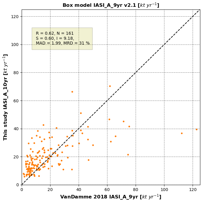
https://www.atmos-chem-phys.net/19/12261/2019/acp-19-12261-2019-f20

Figure E1Comparison of emission estimates using this study's method vs. those obtained using a box model approach of (Van Damme et al., 2018). The individual plots show the comparisons of this study, IASI-A (10-year) emission estimates, using a fixed σ of 15 km and lifetime of 2.5 h vs. the emission estimates obtained using a box model approach on the 9-year (2008–2016) ANNI-NH₃-v2.1 IASI-A dataset. The later emission from Van Damme et al. (2018) have been adjusted to a lifetime of 2.5 h and only locations characterized by a fit with a r>0.3 with the approach used in this study have been kept. R indicates the correlation between the sets, N the number of locations, S and I the resulting slope and intercept of the RMA, MAD and MRD.

Download

https://www.atmos-chem-phys.net/19/12261/2019/acp-19-12261-2019-f21

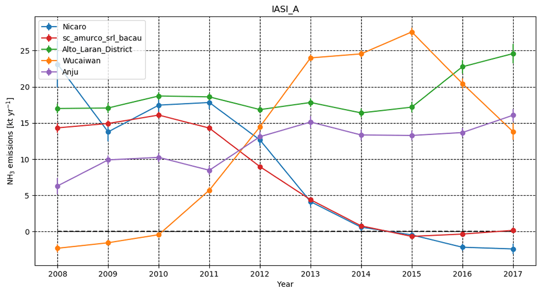
Figure E2Example of IASI-A (2008–2017) 3-year running mean emissions for locations mentioned in Van Damme et al. (2018) using the method used in this study.

Download

Appendix F: Region dimensions

Table F1Summary of regions mentioned in the results.

Download Print Version | Download XLSX

https://www.atmos-chem-phys.net/19/12261/2019/acp-19-12261-2019-f22

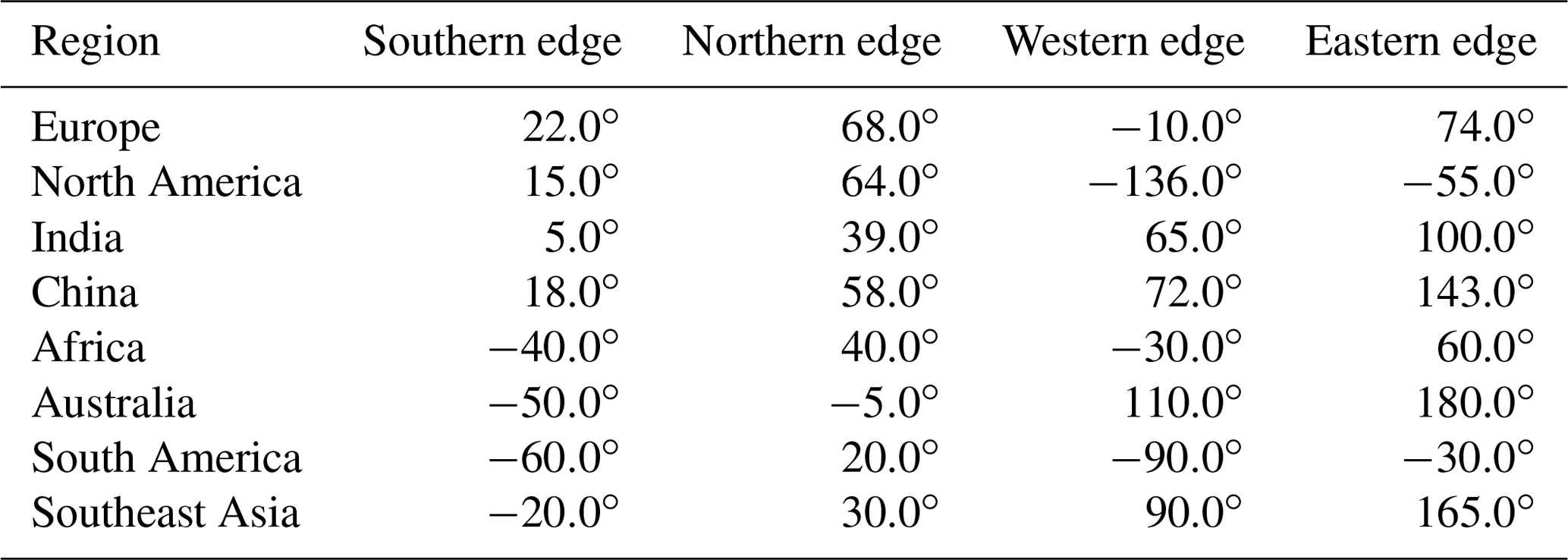
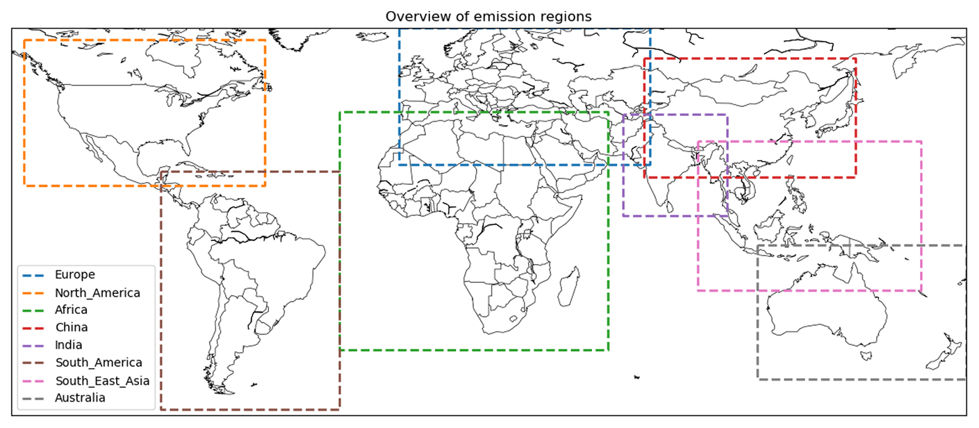
Figure F1Overview of the emission regions.

Supplement

The supplement related to this article is available online at: https://doi.org/10.5194/acp-19-12261-2019-supplement.

Author contributions

ED, DG and CAM worked on the emission methods. MS, KCP, YGM and ED worked on the CrIS retrieval. SvdG worked on the initial set of locations. MVD, SW, LC and PFC produced the IASI-NH₃ dataset. CC produced the IASI-CO dataset. JWE, CAM, MWS, EL, VF and MWS helped interpret the results. The publication was prepared by ED, and all other authors contributed to the discussion of the paper.

Competing interests

The authors declare that they have no conflict of interest.

Acknowledgements

The CrIS input Level1 and Level2 data were obtained from the NOAA Comprehensive Large Array-Data Stewardship System (CLASS) (Liu et al., 2014), with special thanks to Axel Graumann (NOAA). The authors acknowledge the Aeris data infrastructure (https://iasi.aeris-data.fr/nh3/, last access: 13 June 2018) for providing access to the IASI-NH₃ and IASI-CO data used in this study. We thank ECMWF for allowing free use of their meteorological fields. We acknowledge the use of the HTAPv2 dataset http://edgar.jrc.ec.europa.eu/htap_v2/ (last access: 10 December 2017). We thank Jacob Hedelius and Mohit Manocha for the useful discussions.

Review statement

This paper was edited by Qiang Zhang and reviewed by two anonymous referees.

References

ABC News: Clive Palmer's Queensland Nickel goes into voluntary administration, available at: https://www.abc.net.au/news/2016-01-18/qld-nickel-goes-into-voluntary-administration/7094818 (last access: 28 March 2019), 2016. a

ABC News/Ben Millington: Queensland Nickel fined 50K for spills from contaminated tailings dam, available at: https://www.abc.net.au/news/2016-12-14/queensland-nickel-fined-yabulu-nickel-tailings-dam-spills/8121364 (last access: 28 March 2019), 2016. a

Adams, C., McLinden, C. A., Shephard, M. W., Dickson, N., Dammers, E., Chen, J., Makar, P., Cady-Pereira, K. E., Tam, N., Kharol, S. K., Lamsal, L. N., and Krotkov, N. A.: Satellite-derived emissions of carbon monoxide, ammonia, and nitrogen dioxide from the 2016 Horse River wildfire in the Fort McMurray area, Atmos. Chem. Phys., 19, 2577–2599, https://doi.org/10.5194/acp-19-2577-2019, 2019. a, b, c, d, e, f, g

Adams, P. J., Seinfeld, J. H., Koch, D., Mickley, L., and Jacob, D.: General circulation model assessment of direct radiative forcing by the sulfate-nitrate-ammonium-water inorganic aerosol system, J. Geophys. Res.-Atmos., 106, 1097–1111, 2001. a

Battye, W., Aneja, V. P., and Schlesinger, W. H.: Is nitrogen the next carbon?, Earths Future, 5, 894–904, https://doi.org/10.1002/2017EF000592, 2017. a

Beer, R., Shephard, M. W., Kulawik, S. S., Clough, S. A., Eldering, A., Bowman, K. W., Sander, S. P., Fisher, B. M., Payne, V. H., Luo, M., Osterman, G. B., and Worden, J. R.: First satellite observations of lower tropospheric ammonia and methanol, Geophys. Res. Lett., 35, 1–5, https://doi.org/10.1029/2008GL033642, 2008. a

Beirle, S., Boersma, K. F., Platt, U., Lawrence, M. G., and Wagner, T.: Megacity Emissions and Lifetimes of Nitrogen Oxides Probed from Space, Science, 333, 1737–1739, 2011. a

Beirle, S., Hörmann, C., Penning de Vries, M., Dörner, S., Kern, C., and Wagner, T.: Estimating the volcanic emission rate and atmospheric lifetime of SO2 from space: a case study for Kīlauea volcano, Hawai'i, Atmos. Chem. Phys., 14, 8309–8322, https://doi.org/10.5194/acp-14-8309-2014, 2014. a

Bobbink, R., Hicks, K., Galloway, J., Spranger, T., Alkemade, R., Ashmore, M., Bustamante, M., Cinderby, S., Davidson, E., Dentener, F., Emmett, B., Erisman, J. W., Fenn, M., Gilliam, F., Nordin, A., Pardo, L., and De Vries, W.: Global assessment of nitrogen deposition effects on terrestrial plant diversity: A synthesis, Ecol. Appl., 20, 30–59, https://doi.org/10.1890/08-1140.1, 2010. a

Business Review Australia: Queensland Nickel Employees Get Mercedes and Vacations for Christmas, available at: https://web.archive.org/web/20111110040440/http://www.businessreviewaustralia.com/news_archive/tags/clive-palmer/queensland-nickel-employees-get-mercedes-vacations-christmas (last access: 28 March 2019), 2010. a

Castellanos, P., Boersma, K. F., Torres, O., and de Haan, J. F.: OMI tropospheric NO₂ air mass factors over South America: effects of biomass burning aerosols, Atmos. Meas. Tech., 8, 3831–3849, https://doi.org/10.5194/amt-8-3831-2015, 2015. a

ChemStrategy: Venezuela in necessity to produce Urea, available at: https://www.chemstrategy.com.ve/2018/02/urea-production-vzla/ (last access: 28 March 2019), 2018. a

Clarisse, L., Clerbaux, C., Dentener, F., Hurtmans, D., and Coheur, P.-F.: Global ammonia distribution derived from infrared satellite observations, Nat. Geosci., 2, 479–483, https://doi.org/10.1038/ngeo551, 2009. a

Clarisse, L., Van Damme, M., Clerbaux, C., and Coheur, P.-F.: Tracking down global NH₃ point sources with wind-adjusted superresolution, Atmos. Meas. Tech. Discuss., https://doi.org/10.5194/amt-2019-99, in review, 2019. a

Clerbaux, C., Boynard, A., Clarisse, L., George, M., Hadji-Lazaro, J., Herbin, H., Hurtmans, D., Pommier, M., Razavi, A., Turquety, S., Wespes, C., and Coheur, P.-F.: Monitoring of atmospheric composition using the thermal infrared IASI/MetOp sounder, Atmos. Chem. Phys., 9, 6041–6054, https://doi.org/10.5194/acp-9-6041-2009, 2009. a

Coheur, P.-F., Clarisse, L., Turquety, S., Hurtmans, D., and Clerbaux, C.: IASI measurements of reactive trace species in biomass burning plumes, Atmos. Chem. Phys., 9, 5655–5667, https://doi.org/10.5194/acp-9-5655-2009, 2009. a

Copernicus Climate Change Service (C3S): ERA5: Fifth generation of ECMWF atmospheric reanalyses of the global climate, Copernicus Climate Change Service Climate Data Store (CDS), available at: https://cds.climate.copernicus.eu/cdsapp#!/home (last access: 2 March 2018), 2017. a

Crippa, M., Janssens-Maenhout, G., Dentener, F., Guizzardi, D., Sindelarova, K., Muntean, M., Van Dingenen, R., and Granier, C.: Forty years of improvements in European air quality: regional policy-industry interactions with global impacts, Atmos. Chem. Phys., 16, 3825–3841, https://doi.org/10.5194/acp-16-3825-2016, 2016. a

Dammers, E., Palm, M., Van Damme, M., Vigouroux, C., Smale, D., Conway, S., Toon, G. C., Jones, N., Nussbaumer, E., Warneke, T., Petri, C., Clarisse, L., Clerbaux, C., Hermans, C., Lutsch, E., Strong, K., Hannigan, J. W., Nakajima, H., Morino, I., Herrera, B., Stremme, W., Grutter, M., Schaap, M., Wichink Kruit, R. J., Notholt, J., Coheur, P.-F., and Erisman, J. W.: An evaluation of IASI-NH₃ with ground-based Fourier transform infrared spectroscopy measurements, Atmos. Chem. Phys., 16, 10351–10368, https://doi.org/10.5194/acp-16-10351-2016, 2016. a, b

Dammers, E., Schaap, M., Haaima, M., Palm, M., Kruit, R. W., Volten, H., Hensen, A., Swart, D., and Erisman, J.: Measuring atmospheric ammonia with remote sensing campaign: Part 1 – Characterisation of vertical ammonia concentration profile in the centre of The Netherlands, Atmos. Environ., 169, 97–112, https://doi.org/10.1016/j.atmosenv.2017.08.067, 2017a. a, b

Dammers, E., Shephard, M. W., Palm, M., Cady-Pereira, K., Capps, S., Lutsch, E., Strong, K., Hannigan, J. W., Ortega, I., Toon, G. C., Stremme, W., Grutter, M., Jones, N., Smale, D., Siemons, J., Hrpcek, K., Tremblay, D., Schaap, M., Notholt, J., and Erisman, J. W.: Validation of the CrIS fast physical NH₃ retrieval with ground-based FTIR, Atmos. Meas. Tech., 10, 2645–2667, https://doi.org/10.5194/amt-10-2645-2017, 2017b. a, b, c, d, e, f, g

Dee, D. P., Uppala, S. M., Simmons, A. J., Berrisford, P., Poli, P., Kobayashi, S., Andrae, U., Balmaseda, M. A., Balsamo, G., Bauer, P., Bechtold, P., Beljaars, A. C. M., van de Berg, L., Bidlot, J., Bormann, N., Delsol, C., Dragani, R., Fuentes, M., Geer, A. J., Haimberger, L., Healy, S. B., Hersbach, H., Hólm, E. V., Isaksen, L., Kållberg, P., Köhler, M., Matricardi, M., McNally, A. P., Monge-Sanz, B. M., Morcrette, J.-J., Park, B.-K., Peubey, C., de Rosnay, P., Tavolato, C., Thépaut, J.-N., and Vitart, F.: The ERA-Interim reanalysis: configuration and performance of the data assimilation system, Q. J. Roy. Meteor. Soc., 137, 553–597, https://doi.org/10.1002/qj.828, 2011. a

de Foy, B., Wilkins, J. L., Lu, Z., Streets, D. G., and Duncan, B. N.: Model evaluation of methods for estimating surface emissions and chemical lifetimes from satellite data, Atmos. Environ., 98, 66–77, https://doi.org/10.1016/j.atmosenv.2014.08.051, 2014. a, b, c

de Foy, B., Lu, Z., Streets, D. G., Lamsal, L. N., and Duncan, B. N.: Estimates of power plant NO_x emissions and lifetimes from OMI NO₂ satellite retrievals, Atmos. Environ., 116, 1–11, https://doi.org/10.1016/j.atmosenv.2015.05.056, 2015. a

Dentener, F. J. and Crutzen, P. J.: A three-dimensional model of the global ammonia cycle, J. Atmos. Chem., 19, 331–369, https://doi.org/10.1007/BF00694492, 1994. a

de Vries, W., Du, E., and Butterbach-Bahl, K.: Short and long-term impacts of nitrogen deposition on carbon sequestration by forest ecosystems, Curr. Opin. Env. Sust., 9, 90–104, 2014. a

Dimitry Firtash: Gorlovka-based STIROL Concern and Severodonetsk AZOT Halted For Security Reasons, available at: http://en.dmitryfirtash.com/event/gorlovkabased_stirol_concern_and_severodonetsk_azot_halted_for_security_reasons (last access: 28 March 2019), 2014. a

EEA-European Environment Agency: Effects of air pollution on European ecosystems: Past and future exposure of European freshwater and terrestrial habitats to acidifying and eutrophying air pollutants, available at: http://www.eea.europa.eu/data-and-maps/indicators/eea-32-ammonia-nh3-emissions-1/assessment-2 (last access: May 2016), 2014. a

Erisman, J. W. and Schaap, M.: The need for ammonia abatement with respect to secondary PM reductions in Europe, Environ. Pollut., 129, 159–163, https://doi.org/10.1016/j.envpol.2003.08.042, 2004. a

Erisman, J.-W., Vermetten, A. W. M., Asman, W. A. H., Waijers-Ijpelaan, A., and Slanina, J.: Vertical distribution of gases and aerosols: The behaviour of ammonia and related components in the lower atmosphere, Atmos. Environ., 22, 1153–1160, https://doi.org/10.1016/0004-6981(88)90345-9, 1988. a

Erisman, J. W., Bleeker, A., Galloway, J., and Sutton, M. S.: Reduced nitrogen in ecology and the environment, Environ. Pollut., 150, 140–149, https://doi.org/10.1016/j.envpol.2007.06.033, 2007. a

EuroChem Group: Social Responsibility Atlas 2008, available at: http://www.eurochem.ru/wp-content/uploads/2013/02/SR2008.pdf (last access: 28 March 2019), 2008. a

FAO: Survey of Syrian farmers reveals agriculture should be kick-started now despite huge destruction, available at: http://www.fao.org/news/story/en/item/878210/icode/ (last access: 28 March 2019), 2017. a

Fioletov, V., McLinden, C., Krotkov, N., Moran, M., and Yang, K.: Estimation of SO₂ emissions using OMI retrievals, Geophys. Res. Lett., 38, L21811, https://doi.org/10.1029/2011GL049402, 2011. a, b, c

Fioletov, V., McLinden, C., Krotkov, N., and Li, C.: Lifetimes and emissions of SO₂ from point sources estimated from OMI, Geophys. Res. Lett., 42, 1969–1976, 2015. a, b, c, d, e, f, g, h, i, j

Fioletov, V., McLinden, C. A., Kharol, S. K., Krotkov, N. A., Li, C., Joiner, J., Moran, M. D., Vet, R., Visschedijk, A. J. H., and Denier van der Gon, H. A. C.: Multi-source SO₂ emission retrievals and consistency of satellite and surface measurements with reported emissions, Atmos. Chem. Phys., 17, 12597–12616, https://doi.org/10.5194/acp-17-12597-2017, 2017. a, b

Fowler, D., Coyle, M., Skiba, U., Sutton, M. A., Cape, J. N., Reis, S., Sheppard, L. J., Jenkins, A., Grizzetti, B., Galloway, J. N., Vitousek, P., Leach, A., Bouwman, A. F., Butterbach-Bahl, K., Dentener, F., Stevenson, D., Amann, M., and Voss, M.: The global nitrogen cycle in the twenty-first century, Philos. T. R. Soc. B, 368, 20130164, https://doi.org/10.1098/rstb.2013.0164, 2013. a

Fufeng Group: Fufeng Group Limited annual report, available at: http://en.fufeng-group.cn/investor/PdfDetails-40_1.html (last access: 28 March 2019), 2012. a

Gazprom: Company boosts reliability of ammonia production, available at: http://salavat-neftekhim.gazprom.com/press/news/2017/09/44/, (last access: 28 March 2019), 2017. a

George, M., Clerbaux, C., Bouarar, I., Coheur, P.-F., Deeter, M. N., Edwards, D. P., Francis, G., Gille, J. C., Hadji-Lazaro, J., Hurtmans, D., Inness, A., Mao, D., and Worden, H. M.: An examination of the long-term CO records from MOPITT and IASI: comparison of retrieval methodology, Atmos. Meas. Tech., 8, 4313–4328, https://doi.org/10.5194/amt-8-4313-2015, 2015. a

Giannakis, E., Kushta, J., Giannadaki, D., Georgiou, G. K., Bruggeman, A., and Lelieveld, J.: Exploring the economy-wide effects of agriculture on air quality and health: Evidence from Europe, Sci. Total Environ., 663, 889–900, https://doi.org/10.1016/j.scitotenv.2019.01.410, 2019. a

Gyldenkærne, S., Ambelas Skjøth, C., Hertel, O., and Ellermann, T.: A dynamical ammonia emission parameterization for use in air pollution models, J. Geophys. Res.-Atmos., 110, D07108, https://doi.org/10.1029/2004JD005459, 2005. a

Hastings, D. and Dunbar, P.: Global Land One-kilometer Base Elevation (GLOBE) Digital Elevation Model, Documentation, Volume 1.0. Key to Geophysical Records Documentation (KGRD) 34. National Oceanic and Atmospheric Administration, National Geophysical Data Center, 325 Broadway, Boulder, Colorado 80303, USA, 1999. a

Heald, C. L., Collett Jr., J. L., Lee, T., Benedict, K. B., Schwandner, F. M., Li, Y., Clarisse, L., Hurtmans, D. R., Van Damme, M., Clerbaux, C., Coheur, P.-F., Philip, S., Martin, R. V., and Pye, H. O. T.: Atmospheric ammonia and particulate inorganic nitrogen over the United States, Atmos. Chem. Phys., 12, 10295–10312, https://doi.org/10.5194/acp-12-10295-2012, 2012. a

Hickman, J. E., Dammers, E., Galy-Lacaux, C., and van der Werf, G. R.: Satellite evidence of substantial rain-induced soil emissions of ammonia across the Sahel, Atmos. Chem. Phys., 18, 16713–16727, https://doi.org/10.5194/acp-18-16713-2018, 2018. a, b, c, d

Holland, E. A., Dentener, F. J., Braswell, B. H., and Sulzman, J. M.: Contemporary and pre-industrial global reactive nitrogen budgets, Biogeochemistry, 46, 7–43, https://doi.org/10.1007/BF01007572, 1999. a

Hurtmans, D., Coheur, P. F., Wespes, C., Clarisse, L., Scharf, O., Clerbaux, C., Hadji-Lazaro, J., George, M., and Turquety, S.: FORLI radiative transfer and retrieval code for IASI, J. Quant. Spectrosc. Ra., 113, 1391–1408, https://doi.org/10.1016/j.jqsrt.2012.02.036, 2012. a

ICIS: Romania's InterAgro closes last of six fertilizer units, available at: https://www.icis.com/explore/resources/news/2011/05/12/9459467/Articles/2011/04/12/9451925/Romanias-InterAgro-closes-last-of-six-fertilizer-units.html, (last access: 28 March 2019), 2011. a

Jacob, D.: Introduction to atmospheric chemistry, Princeton University Press, Princeton, New Jersey, 1999. a, b

Janssens-Maenhout, G., Crippa, M., Guizzardi, D., Dentener, F., Muntean, M., Pouliot, G., Keating, T., Zhang, Q., Kurokawa, J., Wankmüller, R., Denier van der Gon, H., Kuenen, J. J. P., Klimont, Z., Frost, G., Darras, S., Koffi, B., and Li, M.: HTAP_v2.2: a mosaic of regional and global emission grid maps for 2008 and 2010 to study hemispheric transport of air pollution, Atmos. Chem. Phys., 15, 11411–11432, https://doi.org/10.5194/acp-15-11411-2015, 2015. a

Jones, E., Oliphant, T., Peterson, P., et al.: SciPy: Open source scientific tools for Python, available at: http://www.scipy.org/ (last access: 15 February 2019), 2001. a

Kendall, M. G.: A new measure of rank correlation, Biometrika, 30, 81–93, 1938. a

Kharol, S. K., Shephard, M. W., McLinden, C. A., Zhang, L., Sioris, C. E., O'Brien, J. M., Vet, R., Cady-Pereira, K. E., Hare, E., Siemons, J., and Krotkov, N. A.: Dry Deposition of Reactive Nitrogen From Satellite Observations of Ammonia and Nitrogen Dioxide Over North America, Geophys. Res. Lett., 45, 1157–1166, https://doi.org/10.1002/2017GL075832, 2018. a, b

Krotkov, N. A., McLinden, C. A., Li, C., Lamsal, L. N., Celarier, E. A., Marchenko, S. V., Swartz, W. H., Bucsela, E. J., Joiner, J., Duncan, B. N., Boersma, K. F., Veefkind, J. P., Levelt, P. F., Fioletov, V. E., Dickerson, R. R., He, H., Lu, Z., and Streets, D. G.: Aura OMI observations of regional SO₂ and NO₂ pollution changes from 2005 to 2015, Atmos. Chem. Phys., 16, 4605–4629, https://doi.org/10.5194/acp-16-4605-2016, 2016. a

Kuenen, J. J. P., Visschedijk, A. J. H., Jozwicka, M., and Denier van der Gon, H. A. C.: TNO-MACC_II emission inventory; a multi-year (2003–2009) consistent high-resolution European emission inventory for air quality modelling, Atmos. Chem. Phys., 14, 10963–10976, https://doi.org/10.5194/acp-14-10963-2014, 2014. a, b

Lamsal, L. N., Duncan, B. N., Yoshida, Y., Krotkov, N. A., Pickering, K. E., Streets, D. G., and Lu, Z.: US NO₂ trends (2005–2013): EPA Air Quality System (AQS) data versus improved observations from the Ozone Monitoring Instrument (OMI), Atmos. Environ., 110, 130–143, 2015. a

Lelieveld, J., Evans, J. S., Fnais, M., Giannadaki, D., and Pozzer, A.: The contribution of outdoor air pollution sources to premature mortality on a global scale, Nature, 525, 367, https://doi.org/10.1038/nature15371, 2015. a

Liu, M., Wolf, W., Reale, T., Sharma, A., and Office, N. J. P.: NESDIS-Unique CrIS-ATMS Product System (NUCAPS) Environmental Data Record (EDR) Products, NOAA, https://doi.org/10.7289/v52f7kg5, 2014. a

Lolkema, D. E., Noordijk, H., Stolk, A. P., Hoogerbrugge, R., van Zanten, M. C., and van Pul, W. A. J.: The Measuring Ammonia in Nature (MAN) network in the Netherlands, Biogeosciences, 12, 5133–5142, https://doi.org/10.5194/bg-12-5133-2015, 2015. a

Lonsdale, C. R., Hegarty, J. D., Cady-Pereira, K. E., Alvarado, M. J., Henze, D. K., Turner, M. D., Capps, S. L., Nowak, J. B., Neuman, J. A., Middlebrook, A. M., Bahreini, R., Murphy, J. G., Markovic, M. Z., VandenBoer, T. C., Russell, L. M., and Scarino, A. J.: Modeling the diurnal variability of agricultural ammonia in Bakersfield, California, during the CalNex campaign, Atmos. Chem. Phys., 17, 2721–2739, https://doi.org/10.5194/acp-17-2721-2017, 2017. a

Lutsch, E., Dammers, E., Conway, S., and Strong, K.: Long-range transport of NH₃, CO, HCN, and C₂H₆ from the 2014 Canadian Wildfires, Geophys. Res. Lett., 43, 8286–8297, https://doi.org/10.1002/2016GL070114, 2016. a, b

Mann, H. B.: Nonparametric tests against trend, Econometrica, Journal of the Econometric Society, 245–259, 1945. a

Martin, R. V.: Satellite remote sensing of surface air quality, Atmos. Environ., 42, 7823–7843, https://doi.org/10.1016/j.atmosenv.2008.07.018, 2008. a

McLinden, C. A., Fioletov, V., Shephard, M. W., Krotkov, N., Li, C., Martin, R. V., Moran, M. D., and Joiner, J.: Space-based detection of missing sulfur dioxide sources of global air pollution, Nat. Geosci., 9, 496, https://doi.org/10.1038/ngeo2724, 2016. a, b, c, d

Mebust, A. K., Russell, A. R., Hudman, R. C., Valin, L. C., and Cohen, R. C.: Characterization of wildfire NO_x emissions using MODIS fire radiative power and OMI tropospheric NO₂ columns, Atmos. Chem. Phys., 11, 5839–5851, https://doi.org/10.5194/acp-11-5839-2011, 2011. a, b

Moncet, J.-L., Uymin, G., Lipton, A. E., and Snell, H. E.: Infrared radiance modeling by optimal spectral sampling, J. Atmos. Sci., 65, 3917–3934, 2008. a

Myhre, G., Shindell, D., Bréon, F.-M., Collins, W., Fuglestvedt, J., Huang, J., Koch, D., Lamarque, J.-F., Lee, D., Mendoza, B., and Nakajima, T.: Anthropogenic and natural radiative forcing, Climate Change, 423, 658–740, 2013. a

Nassar, R., Hill, T. G., McLinden, C. A., Wunch, D., Jones, D. B., and Crisp, D.: Quantifying CO₂ emissions from individual power plants from space, Geophys. Res. Lett., 44, 10–045, 2017. a, b

Nowak, J., Neuman, J., Bahreini, R., Middlebrook, A., Holloway, J., McKeen, S., Parrish, D., Ryerson, T., and Trainer, M.: Ammonia sources in the California South Coast Air Basin and their impact on ammonium nitrate formation, Geophys. Res. Lett., 39, L07804, https://doi.org/10.1029/2012GL051197, 2012. a

Oren, R., Ellsworth, D. S., Johnsen, K. H., Phillips, N., Ewers, B. E., Maier, C., Schäfer, K. V., McCarthy, H., Hendrey, G., McNulty, S. G., and Katul, G. G.: Soil fertility limits carbon sequestration by forest ecosystems in a CO 2-enriched atmosphere, Nature, 411, 469–472, https://doi.org/10.1038/35078064, 2001. a

Pommier, M., McLinden, C. A., and Deeter, M.: Relative changes in CO emissions over megacities based on observations from space, Geophys. Res. Lett., 40, 3766–3771, https://doi.org/10.1002/grl.50704, 2013. a, b

Pope III, C. A., Burnett, R. T., Thun, M. J., Calle, E. E., Krewski, D., Ito, K., and Thurston, G. D.: Lung cancer, cardiopulmonary mortality, and long-term exposure to fine particulate air pollution, JAMA, 287, 1132–1141, 2002. a

Pope III, C. A., Ezzati, M., and Dockery, D. W.: Fine-particulate air pollution and life expectancy in the United States, New Engl. J. Med., 360, 376–386, 2009. a

R'Honi, Y., Clarisse, L., Clerbaux, C., Hurtmans, D., Duflot, V., Turquety, S., Ngadi, Y., and Coheur, P.-F.: Exceptional emissions of NH₃ and HCOOH in the 2010 Russian wildfires, Atmos. Chem. Phys., 13, 4171–4181, https://doi.org/10.5194/acp-13-4171-2013, 2013. a, b, c, d

Rockstrom, J., Steffen, W., Noone, K., Persson, A., Chapin, F. S., Lambin, E. F., Lenton, T. M., Scheffer, M., Folke, C., Schellnhuber, H. J., Nykvist, B., de Wit, C. A., Hughes, T., van der Leeuw, S., Rodhe, H., Sorlin, S., Snyder, P. K., Costanza, R., Svedin, U., Falkenmark, M., Karlberg, L., Corell, R. W., Fabry, V. J., Hansen, J., Walker, B., Liverman, D., Richardson, K., Crutzen, P., and Foley, J. A.: A safe operating space for humanity, Nature, 461, 472–475, https://doi.org/10.1038/461472a, 2009. a

Rodgers, C. D.: Inverse Methods for Atmospheric Sounding – Theory and Practice, 2, 256, https://doi.org/10.1142/9789812813718, 2000. a

Schaap, M., van Loon, M., ten Brink, H. M., Dentener, F. J., and Builtjes, P. J. H.: Secondary inorganic aerosol simulations for Europe with special attention to nitrate, Atmos. Chem. Phys., 4, 857–874, https://doi.org/10.5194/acp-4-857-2004, 2004. a

Schiferl, L. D., Heald, C. L., Nowak, J. B., Holloway, J. S., Neuman, J. A., Bahreini, R., Pollack, I. B., Ryerson, T. B., Wiedinmyer, C., and Murphy, J. G.: An investigation of ammonia and inorganic particulate matter in California during the CalNex campaign, J. Geophys. Res.-Atmos., 119, 1883–1902, https://doi.org/10.1002/2013JD020765, 2014. a

Schiferl, L. D., Heald, C. L., Van Damme, M., Clarisse, L., Clerbaux, C., Coheur, P.-F., Nowak, J. B., Neuman, J. A., Herndon, S. C., Roscioli, J. R., and Eilerman, S. J.: Interannual variability of ammonia concentrations over the United States: sources and implications, Atmos. Chem. Phys., 16, 12305–12328, https://doi.org/10.5194/acp-16-12305-2016, 2016. a

Schrader, F., Schaap, M., Zöll, U., Kranenburg, R., and Brümmer, C.: The hidden cost of using low-resolution concentration data in the estimation of NH₃ dry deposition fluxes, Sci. Rep.-IK, 8, 969, https://doi.org/10.1038/s41598-017-18021-6, 2018. a

Seinfeld, J. H. and Pandis, S. N.: Atmospheric chemistry and physics: from air pollution to climate change, John Wiley & Sons, New York, 2012. a

Sen, P. K.: Estimates of the regression coefficient based on Kendall's tau, J. Am. Stat. Assoc., 63, 1379–1389, 1968. a

Shephard, M. W. and Cady-Pereira, K. E.: Cross-track Infrared Sounder (CrIS) satellite observations of tropospheric ammonia, Atmos. Meas. Tech., 8, 1323–1336, https://doi.org/10.5194/amt-8-1323-2015, 2015. a, b, c, d, e, f

Shephard, M. W., Cady-Pereira, K. E., Luo, M., Henze, D. K., Pinder, R. W., Walker, J. T., Rinsland, C. P., Bash, J. O., Zhu, L., Payne, V. H., and Clarisse, L.: TES ammonia retrieval strategy and global observations of the spatial and seasonal variability of ammonia, Atmos. Chem. Phys., 11, 10743–10763, https://doi.org/10.5194/acp-11-10743-2011, 2011. a

Shephard, M., Dammers, E., Cady-Pereira, K. E., Kharol, S. K., Thompson, J., Gainariu-Matz, Y., Zhang, J., McLinden, C. A., Kovachik, A., Moran, M., Bittman, S., Sioris, C., Griffin, D., Alvarado, M. J., Lonsdale, C., Savic-Jovcic, V., and Zheng, Q.: Ammonia measurements from space with the Cross-track Infrared Sounder (CrIS): characteristics and applications, Atmos. Chem. Phys. Discuss., https://doi.org/10.5194/acp-2019-705, in review, 2019. a, b, c, d

Sheppard, S. C., Bittman, S., and Bruulsema, T. W.: Monthly ammonia emissions from fertilizers in 12 Canadian Ecoregions, Can. J. Soil Sci., 90, 113–127, https://doi.org/10.4141/CJSS09006, 2010. a

Sommer, S. G., Olesen, J. E., and Christensen, B. T.: Effects of temperature, wind speed and air humidity on ammonia volatilization from surface applied cattle slurry, J. Agr. Sci., 117, 91–100, 1991. a

Stieb, D. M., Chen, L., Eshoul, M., and Judek, S.: Ambient air pollution, birth weight and preterm birth: A systematic review and meta-analysis, Environ. Res., 117, 100–111, https://doi.org/10.1016/j.envres.2012.05.007, 2012. a

Streets, D. G., Canty, T., Carmichael, G. R., de Foy, B., Dickerson, R. R., Duncan, B. N., Edwards, D. P., Haynes, J. A., Henze, D. K., Houyoux, M. R., and Jacob, D. J.: Emissions estimation from satellite retrievals: A review of current capability, Atmos. Environ., 77, 1011–1042, 2013. a

Sutton, M. A., Reis, S., and Baker, S. M.: Atmospheric ammonia, Detecting Emission Changes and Environmental Impacts, 494, New York, ISBN 978-1-4020-9120-9, 2009. a

Tevlin, A. G., Li, Y., Collett, J. L., McDuffie, E. E., Fischer, E. V., and Murphy, J. G.: Tall Tower Vertical Profiles and Diurnal Trends of Ammonia in the Colorado Front Range, J. Geophys. Res.-Atmos., 122, 12468–12487, https://doi.org/10.1002/2017JD026534, 2017. a, b

Van Damme, M., Clarisse, L., Heald, C. L., Hurtmans, D., Ngadi, Y., Clerbaux, C., Dolman, A. J., Erisman, J. W., and Coheur, P. F.: Global distributions, time series and error characterization of atmospheric ammonia (NH₃) from IASI satellite observations, Atmos. Chem. Phys., 14, 2905–2922, https://doi.org/10.5194/acp-14-2905-2014, 2014a. a, b, c, d, e, f, g

Van Damme, M., Wichink Kruit, R. J., Schaap, M., Clarisse, L., Clerbaux, C., and Coheur, P. F.: Evaluating 4 years of atmospheric ammonia (NH₃) over Europe using IASI satellite observations and LOTOS-EUROS model results, J. Geophys. Res.-Atmos., 119, 1–18, https://doi.org/10.1002/2014JD021911, 2014b. a, b

Van Damme, M., Clarisse, L., Dammers, E., Liu, X., Nowak, J. B., Clerbaux, C., Flechard, C. R., Galy-Lacaux, C., Xu, W., Neuman, J. A., Tang, Y. S., Sutton, M. A., Erisman, J. W., and Coheur, P. F.: Towards validation of ammonia (NH₃) measurements from the IASI satellite, Atmos. Meas. Tech., 8, 1575–1591, https://doi.org/10.5194/amt-8-1575-2015, 2015. a, b

Van Damme, M., Whitburn, S., Clarisse, L., Clerbaux, C., Hurtmans, D., and Coheur, P.-F.: Version 2 of the IASI NH₃ neural network retrieval algorithm: near-real-time and reanalysed datasets, Atmos. Meas. Tech., 10, 4905–4914, https://doi.org/10.5194/amt-10-4905-2017, 2017. a, b, c, d

Van Damme, M., Clarisse, L., Whitburn, S., Hadji-Lazaro, J., Hurtmans, D., Clerbaux, C., and Coheur, P.-F.: Industrial and agricultural ammonia point sources exposed, Nature, 564, 99–103, https://doi.org/10.1038/s41586-018-0747-1, 2018. a, b, c, d, e, f, g, h, i, j, k, l, m, n, o, p, q, r, s, t, u

Van Zanten, M., Kruit, R. W., Hoogerbrugge, R., Van der Swaluw, E., and Van Pul, W.: Trends in ammonia measurements in the Netherlands over the period 1993–2014, Atmos. Environ., 148, 352–360, 2017. a

Warner, J. X., Wei, Z., Strow, L. L., Dickerson, R. R., and Nowak, J. B.: The global tropospheric ammonia distribution as seen in the 13-year AIRS measurement record, Atmos. Chem. Phys., 16, 5467–5479, https://doi.org/10.5194/acp-16-5467-2016, 2016. a

Warner, J. X., Dickerson, R. R., Wei, Z., Strow, L. L., Wang, Y., and Liang, Q.: Increased atmospheric ammonia over the world's major agricultural areas detected from space, Geophys. Res. Lett., 44, 2875–2884, https://doi.org/10.1002/2016GL072305, 2017. a, b, c, d

Whitburn, S., Van Damme, M., Kaiser, J., van der Werf, G., Turquety, S., Hurtmans, D., Clarisse, L., Clerbaux, C., and Coheur, P.-F.: Ammonia emissions in tropical biomass burning regions: Comparison between satellite-derived emissions and bottom-up fire inventories, Atmos. Environ., 121, 42–54, https://doi.org/10.1016/j.atmosenv.2015.03.015, 2015. a, b, c, d, e

Whitburn, S., Van Damme, M., Clarisse, L., Bauduin, S., Heald, C., Hadji-Lazaro, J., Hurtmans, D., Zondlo, M., Clerbaux, C., and Coheur, P.-F.: A flexible and robust neural network IASI-NH₃ retrieval algorithm, J. Geophys. Res.-Atmos., 121, 6581–6599, https://doi.org/10.1002/2016JD024828, 2016a. a, b

Whitburn, S., Van Damme, M., Clarisse, L., Turquety, S., Clerbaux, C., and Coheur, P.-F.: Doubling of annual ammonia emissions from the peat fires in Indonesia during the 2015 El Niño, Geophys. Res. Lett., 43, 11007–11014, https://doi.org/10.1002/2016GL070620, 2016b. a, b

Wichink Kruit, R., Aben, J., de Vries, W., Sauter, F., van der Swaluw, E., van Zanten, M., and van Pul, W.: Modelling trends in ammonia in the Netherlands over the period 1990–2014, Atmos. Environ., 154, 20–30, https://doi.org/10.1016/j.atmosenv.2017.01.031, 2017. a, b

Xu, W., Song, W., Zhang, Y., Liu, X., Zhang, L., Zhao, Y., Liu, D., Tang, A., Yang, D., Wang, D., Wen, Z., Pan, Y., Fowler, D., Collett Jr., J. L., Erisman, J. W., Goulding, K., Li, Y., and Zhang, F.: Air quality improvement in a megacity: implications from 2015 Beijing Parade Blue pollution control actions, Atmos. Chem. Phys., 17, 31–46, https://doi.org/10.5194/acp-17-31-2017, 2017. a

Yao, X. and Zhang, L.: Trends in atmospheric ammonia at urban, rural, and remote sites across North America, Atmos. Chem. Phys., 16, 11465–11475, https://doi.org/10.5194/acp-16-11465-2016, 2016. a

Yokelson, R. J., Crounse, J. D., DeCarlo, P. F., Karl, T., Urbanski, S., Atlas, E., Campos, T., Shinozuka, Y., Kapustin, V., Clarke, A. D., Weinheimer, A., Knapp, D. J., Montzka, D. D., Holloway, J., Weibring, P., Flocke, F., Zheng, W., Toohey, D., Wennberg, P. O., Wiedinmyer, C., Mauldin, L., Fried, A., Richter, D., Walega, J., Jimenez, J. L., Adachi, K., Buseck, P. R., Hall, S. R., and Shetter, R.: Emissions from biomass burning in the Yucatan, Atmos. Chem. Phys., 9, 5785–5812, https://doi.org/10.5194/acp-9-5785-2009, 2009. a, b

Zhang, L., Chen, Y., Zhao, Y., Henze, D. K., Zhu, L., Song, Y., Paulot, F., Liu, X., Pan, Y., Lin, Y., and Huang, B.: Agricultural ammonia emissions in China: reconciling bottom-up and top-down estimates, Atmos. Chem. Phys., 18, 339–355, https://doi.org/10.5194/acp-18-339-2018, 2018. a, b

Zhang, Y., Tang, A., Wang, D., Wang, Q., Benedict, K., Zhang, L., Liu, D., Li, Y., Collett Jr., J. L., Sun, Y., and Liu, X.: The vertical variability of ammonia in urban Beijing, China, Atmos. Chem. Phys., 18, 16385–16398, https://doi.org/10.5194/acp-18-16385-2018, 2018. a, b

Zhu, L., Henze, D. K., Cady-Pereira, K. E., Shephard, M. W., Luo, M., Pinder, R. W., Bash, J. O., and Jeong, G. R.: Constraining U.S. ammonia emissions using TES remote sensing observations and the GEOS-Chem adjoint model, J. Geophys. Res.-Atmos., 118, 3355–3368, https://doi.org/10.1002/jgrd.50166, 2013. a, b

Zöll, U., Brümmer, C., Schrader, F., Ammann, C., Ibrom, A., Flechard, C. R., Nelson, D. D., Zahniser, M., and Kutsch, W. L.: Surface–atmosphere exchange of ammonia over peatland using QCL-based eddy-covariance measurements and inferential modeling, Atmos. Chem. Phys., 16, 11283–11299, https://doi.org/10.5194/acp-16-11283-2016, 2016. a

NH3 emissions from large point sources derived from CrIS and IASI satellite observations

2.1 Satellite products

2.1.1 CrIS

2.1.2 IASI

2.2 NH3 emission inventories and source locations

2.3 Meteorology

2.4 Data criteria

2.5 Method and uncertainties

2.5.1 Wind rotation and fitting algorithm

2.5.2 Method uncertainty and detection limit

Satellite total columns

Diurnal and seasonal emission cycles

Fitting algorithm

Meteorology

Detection limit

3.1 Lifetime and emission fits

3.2 Constrained fits and comparison

3.3 Emission time series

NH₃ emissions from large point sources derived from CrIS and IASI satellite observations

2.2 NH₃ emission inventories and source locations