the Creative Commons Attribution 4.0 License.
the Creative Commons Attribution 4.0 License.
 | 02 Oct 2019
Controls on the water vapor isotopic composition near the surface of tropical oceans and role of boundary layer mixing processes
Joseph Galewsky
Gilles Reverdin
Florent Brient
Understanding what controls the water vapor isotopic composition of the sub-cloud layer (SCL) over tropical oceans (δD0) is a first step towards understanding the water vapor isotopic composition everywhere in the troposphere. We propose an analytical model to predict δD0 motivated by the hypothesis that the altitude from which the free tropospheric air originates (zorig) is an important factor: when the air mixing into the SCL is lower in altitude, it is generally moister, and thus it depletes the SCL more efficiently. We extend previous simple box models of the SCL by prescribing the shape of δD vertical profiles as a function of humidity profiles and by accounting for rain evaporation and horizontal advection effects. The model relies on the assumption that δD profiles are steeper than mixing lines, and that the SCL is at steady state, restricting its applications to timescales longer than daily. In the model, δD0 is expressed as a function of zorig, humidity and temperature profiles, surface conditions, a parameter describing the steepness of the δD vertical gradient, and a few parameters describing rain evaporation and horizontal advection effects. We show that δD0 does not depend on the intensity of entrainment, in contrast to several previous studies that had hoped that δD0 measurements could help estimate this quantity.
Based on an isotope-enabled general circulation model simulation, we show that δD0 variations are mainly controlled by mid-tropospheric depletion and rain evaporation in ascending regions and by sea surface temperature and zorig in subsiding regions. In turn, could δD0 measurements help estimate zorig and thus discriminate between different mixing processes? For such isotope-based estimates of zorig to be useful, we would need a precision of a few hundred meters in deep convective regions and smaller than 20 m in stratocumulus regions. To reach this target, we would need daily measurements of δD in the mid-troposphere and accurate measurements of δD0 (accuracy down to 0.1 ‰ in the case of stratocumulus clouds, which is currently difficult to obtain). We would also need information on the horizontal distribution of δD to account for horizontal advection effects, and full δD profiles to quantify the uncertainty associated with the assumed shape for δD profiles. Finally, rain evaporation is an issue in all regimes, even in stratocumulus clouds. Innovative techniques would need to be developed to quantify this effect from observations.


1.1 What controls the water vapor isotopic composition?
The water vapor isotopic composition (e.g., expressed in per mill, where R is the D∕H ratio and SMOW is the Standard Mean Ocean Water reference), has been shown to be sensitive to a wide range of atmospheric processes (Galewsky et al., 2016), such as continental recycling (Salati et al., 1979; Risi et al., 2013); unsaturated downdrafts (Risi et al., 2008, 2010a); rain evaporation (Worden et al., 2007; Field et al., 2010); the degree of organization of convection (Lawrence et al., 2004; Tremoy et al., 2014); the convective depth (Lacour et al., 2017b); the proportion of precipitation that occurs as convective or large-scale precipitation (Lee et al., 2009; Kurita, 2013; Aggarwal et al., 2016); vertical mixing in the lower troposphere (Benetti et al., 2015; Galewsky, 2018a, b), mid-troposphere (Risi et al., 2012b) or upper-troposphere (Galewsky and Samuels-Crow, 2014); convective detrainment (Moyer et al., 1996; Webster and Heymsfield, 2003); and ice microphysics (Bolot et al., 2013). It is therefore very challenging to quantitatively understand what controls the isotopic composition of water vapor.
A first step towards this goal is to understand what controls the water vapor isotopic composition in the sub-cloud layer (SCL) of tropical (30∘ S–30∘ N) oceans. Indeed, this water vapor is an important source moistening air masses traveling to land regions (Gimeno et al., 2010; Ent and Savenije, 2013) and towards higher latitudes (Ciais et al., 1995; Delaygue et al., 2000). It is also ultimately the only source of water vapor in the tropical free troposphere since water vapor in the free troposphere ultimately originates from convective detrainment (Sherwood, 1996), and convection ultimately feeds from the SCL air (Bony et al., 2008). Therefore, the water vapor isotopic composition in the SCL of tropical oceans serves as initial conditions to understand the isotopic composition in land waters and in the tropospheric water vapor everywhere on Earth. We focus here on the SCL because, by definition, there is no complication by cloud condensation processes.
The goal of this paper is thus to propose a simple analytical equation that allows us to understand and quantify the factors controlling the δD in the water vapor in the SCL of tropical oceans. So far, the most famous analytical equation for this purpose has been the closure equation developed by Merlivat and Jouzel (1979) (MJ79). This closure equation can be derived by assuming that all the water vapor in the SCL air originates from surface evaporation. The water balance of the SCL can be closed by assuming a mass export at the SCL top (e.g., by convective mass fluxes) and a totally dry entrainment into the SCL to compensate for this mass export. The MJ79 equation has proven very useful to capture the sensitivity of δD and second-order parameter d-excess to sea surface conditions (Merlivat and Jouzel, 1979; Ciais et al., 1995; Risi et al., 2010d). However, the δD calculated from this equation suffers from a high bias in tropical regions (Jouzel and Koster, 1996). This bias can be explained by the neglect of vertical mixing between the SCL and air entrained from the free troposphere (FT). The MJ79 equation can better reproduce surface water vapor observation when extended to take into account this mixing (Benetti et al., 2015, hereafter B15). This extension requires us to know the specific humidity (q) and water vapor δD of the entrained air. To get these values, they assume that the air entrained into the boundary layer comes from a constant altitude. However, this does not reflect the complexity of entrainment and mixing processes in marine boundary layers.
1.2 Entrainment and mixing mechanisms
Figure 1 summarizes our knowledge about these entrainment and mixing processes. In stratocumulus regions, clouds are thin and the inversion is just above the lifting condensation level (LCL). Air is entrained from the FT by cloud-top entrainment driven by radiative cooling or wind shear instabilities (Mellado, 2017), possibly amplified by evaporative cooling of droplets (Lozar and Mellado, 2015). Both direct numerical simulations (Mellado, 2017) and observations of tracers (Faloona et al., 2005) and cloud holes (Gerber et al., 2005) show that air is entrained from a thin layer above the inversion, thinner than 80 m and as small as 5 m. The boundary layer itself is animated by updrafts, downdrafts, and associated turbulent shells that bring air from the cloud layer downward (Brient et al., 2019; Davini et al., 2017).
In trade-wind cumulus regions, the cloudy layer is a bit deeper. Observational studies and large-eddy simulations have pointed out the important role of thin subsiding shells around cumulus clouds, driven by cloud-top radiative cooling, mixing, and evaporative cooling of droplets (Jonas, 1990; Rodts et al., 2003; Heus and Jonker, 2008; Heus et al., 2009; Park et al., 2016). This brings air from the cloudy layer to the SCL. Subsiding shells may also cover overshooting plumes of the cumulus clouds, entraining FT air into the cloud layer (Heus and Jonker, 2008).
In deep convective regions, unsaturated downdrafts driven by rain evaporation (Zipser, 1977) are known to contribute significantly to the energy budget of the SCL (Emanuel et al., 1994). Large-eddy simulations show that subsiding shells, similar to those documented in shallow convection, also exist around deep convective clouds (Glenn and Krueger, 2014). In the clear-sky environment between clouds, turbulent entrainment into the SCL may also play a significant role (Thayer-Calder and Randall, 2015).
Therefore, whatever the cloud regime, air entering the SCL from above may originate from either the cloud layer or the free troposphere, depending on the mixing mechanism. Therefore, in this paper in contrast with B15, we let the altitude from which the air originates, zorig, be variable. We do not call it “entrained” air because entrainment sometimes refers to mixing processes through an interface (e.g., De Rooy et al., 2013; Davini et al., 2017), whereas air in the SCL may also enter through deep, coherent, and penetrative structures such as unsaturated downdrafts. We do not call it FT air either since it may originate from the cloudy layer.
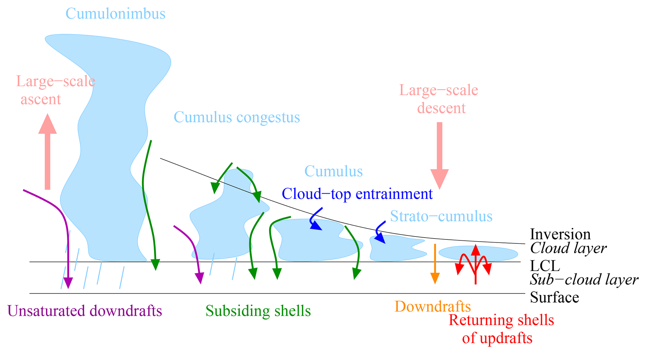
Figure 1Schematics showing the different types of clouds and mixing processes as a function of the large-scale circulation.
1.3 Goal of the article
To acknowledge the diversity and complexity of mixing mechanisms, we extend the B15 framework in several ways. First, we assume that we know the shape of δD profiles as a function of q. Second, we write the specific humidity of the air originating from above the SCL as a function of zorig. Third, we account for rain evaporation and horizontal effects.
While B15 focused on observations during a field campaign, we also apply the extended equation to global outputs of an isotope-enabled general circulation model, with the aim to quantify the different factors controlling the δD variability in the tropics. The variable zorig will emerge as an important factor. Therefore, we discuss the possibility that δD measurements at the near surface and through the lower FT could help estimate zorig and thus the mixing processes between the SCL and the air above.
Note that we focus on δD only. Results for δ18O are similar. We do not aim at capturing the second-order parameter d-excess because our model requires some knowledge about free-tropospheric vertical profiles of isotopic composition. While δD is known to decrease with altitude (Ehhalt, 1974; Ehhalt et al., 2005; Sodemann et al., 2017), vertical profiles of d-excess are more diverse and less well understood (Sodemann et al., 2017). In addition, there is more need for an extension of MJ79 for δD than for d-excess since the effect of convective mixing is larger on δD than on d-excess (Risi et al., 2010d; Benetti et al., 2014).
2.1 Box model and budget equations
Building on Benetti et al. (2014) and B15, we consider a simple box representing the SCL (Fig. 2). We assume that the air comes from above (M) and from the incoming large-scale horizontal advection (Fadv) and is exported through the SCL top (N, e.g., turbulent mixing or convective mass flux) and by outgoing large-scale horizontal advection (Fadv,out). We assume that the SCL is at steady state. For example, its depth is constant. Since the SCL properties may exhibit a diurnal cycle (Duynkerke et al., 2004), this hypothesis restricts the application of this model to timescales longer than daily. The air mass budget of the SCL is thus
These fluxes also transport water vapor and isotopes. In addition, surface evaporation E and rain evaporation Fevap import water vapor and isotopes (Fig. 2).
Hereafter, to simplify equations, we use the isotopic ratio R instead of δD.
The SCL is usually well mixed (Betts and Ridgway, 1989; Stevens, 2006; De Roode et al., 2016). We thus assume that the humidity and isotopic properties are constant vertically and horizontally in the SCL. They are noted (q0, R0). The humidity and isotopic properties of the mass flux export N are thus also (q0, R0). The properties of the flux M are noted (qorig, Rorig). The properties of the incoming air by horizontal advection are noted (qadv, Radv). For simplicity here we neglect the effect of horizontal gradients in humidity (i.e., qadv=q0), assuming that the main effect of horizontal advection on δD0 arises from horizontal gradients in δD. Appendix C explains how Radv can be calculated. At steady state, the water budget of the SCL is written
This model is consistent with SCL water budgets that have already been derived in previous studies (Bretherton et al., 1995), except that we consider steady state. This equation can be solved for q0:
The SCL humidity q0 is thus sensitive to M, justifying that it can be used to estimate the mixing intensity or the “entrainment velocity” (ρ being the air volumic mass) (Bretherton et al., 1995).
At steady state, the water isotope budget of the SCL is written
where RE is the isotopic composition of the surface evaporation. It is assumed to follow the Craig and Gordon (1965) equation:
where Roce is the isotopic ratio in the surface ocean water, αeq is the equilibrium fractionation calculated at the sea surface temperature (SST) (Majoube, 1971), αK is the kinetic fractionation coefficient (MJ79), and h0 is the relative humidity normalized at the SST (, where qs is the saturation-specific humidity at SST and P0 is the surface pressure).
We write the isotopic composition of the rain evaporation, Revap, as
where αevap is an effective fractionation coefficient. For example, if droplets are formed near the cloud base, some of them precipitate and evaporate totally into the SCL (e.g., in non-precipitating shallow cumulus clouds), then αevap=α(Tcloud base). In contrast, if droplets are formed in deep convective updrafts after total condensation of the SCL vapor, and then a very small fraction of the rain is evaporated into a very dry SCL, then (Stewart, 1975).
We note the ratio of water vapor coming from rain evaporation to that of surface evaporation, and the ratio of water vapor coming from horizontal advection to that coming from surface evaporation. We note the ratio of isotopic ratios of horizontal advection to that of the SCL.
Note that in all our equations, we assume that temperature and humidity profiles and all basic surface meteorological variables are known. We do not attempt to express either h0 as a function of q0 as in B15 or the q profile as a function of q0. Our ultimate goal is to assess the added value of δD assuming that meteorological measurements are already routinely performed.
By combining all these equations, we get
where is the proportion of the water vapor in the SCL that originates from above.
An intriguing aspect of this equation is that the sensitivity to M disappears. In contrast to q0, R0 is not sensitive to M. Therefore, it appears illusory to promise that water vapor isotopic measurements could help constrain the entrainment velocity that many studies have striven to estimate (Nicholls and Turton, 1986; Khalsa, 1993; Wang and Albrecht, 1994; Bretherton et al., 1995; Faloona et al., 2005; Gerber et al., 2005, 2013). The lack of sensitivity of R0 to M is explained physically by the fact that for a given q0 and qorig, if M increases, then E+Fevap increases in the same proportion to maintain the water balance. Therefore, the relative proportion of the water vapor originating from surface and rain evaporation to that coming from above, to which R0 is sensitive, remains constant. Rather, since q and R vary with altitude, R0 is sensitive to the altitude from which the air originates.

Figure 2Schematics showing the simple box model on which the theoretical framework is based, and illustrating the main notations.
2.2 Closure if δD profile follows a Rayleigh distillation line
Equation (6) requires knowing qorig and Rorig. B15 take these values from general circulation model (GCM) outputs at 700 hPa. In contrast, here we acknowledge the diversity and complexity of mixing mechanisms by keeping the possibility to take qorig and Rorig at a variable altitude zorig.
If the goal is to predict R0 from zorig, we can apply Eq. (6) if we know the q and δD vertical profiles. Conversely, if the goal is to predict zorig from R0, we can numerically solve Eq. (6) if we know the q and δD vertical profiles. No analytical solution exists in the general case, but a numerical solution can be searched for the zorig based on Eq. (6). However, the existence and unicity of the solution is not warranted for all kinds of profiles (e.g., Appendix A).
In practice, full isotopic profiles are costly to measure. In addition, our goal is to develop an analytical model. Therefore, in the following we simplify the problem by assuming that the vertical profile of R follows a known relationship as a function of q. Measured vertical profiles of δD are usually bounded by two curves when plotted in a (q, δD) diagram (Sodemann et al., 2017): Rayleigh distillation curve and mixing line.
First, we explore the case of a Rayleigh distillation curve (Dansgaard, 1964), as in Galewsky and Rabanus (2016):
where αeff is an effective fractionation coefficient. Typically, q decreases with altitude, so R also decreases with altitude. However, in observations and models, vertical profiles of R can be very diverse (Bony et al., 2008; Sodemann et al., 2017). The water vapor may be more (Worden et al., 2007) or less (Sodemann et al., 2017) depleted than predicted by a Rayleigh curve using a realistic fractionation factor that depends on local temperature. Therefore, here we let αeff be a free parameter larger than 1. Rather than assuming a true Rayleigh curve, we simply assume that R and q are logarithmically related. Effects of horizontal advection and rain evaporation on tropospheric profiles are encapsulated into αeff.
Injecting Eq. (7) into Eq. (6), we get
A simpler form can be found if neglecting horizontal advection and rain evaporation effects ():
As a consistency check, in the limit case where the air coming from above is totally dry (rorig=0), Eq. (9) becomes the MJ79 equation:
Equation (8) tells us that whenever αeff>1, R0 decreases as rorig increases (Fig. 3 red), i.e., as qorig is moister. Therefore, R0 decreases as zorig is lower in altitude. This result may be counterintuitive, but can be physically interpreted as follows. If zorig is high, mixing brings air with very depleted water vapor, but since the air is dry, the depleting effect is small. In contrast, if zorig is low, mixing brings air with water vapor that is not very depleted, but since the air is moist, the depleting effect is large (Fig. 4a).
Figure 3 (red) shows that the range of possible δD values is restricted to −70 ‰ to −85 ‰. This explains why in quiescent conditions near the sea level in tropical ocean locations, the water vapor δD varies little (Benetti et al. (2014), Françoise Vimeux, personal communication, 2018). In the limit case where rorig→1 (i.e., the air comes from the SCL top), (L'Hôpital's rule was used to calculate this limit). This lower bound is not so depleted compared to the more depleted water vapor observed in regions of deep convection (e.g., Lawrence et al., 2002, 2004; Kurita, 2013). This is because when rorig→1, the water vapor coming from above has a composition very close to that of the SCL, so the depleting effect is limited. In addition, surface evaporation strongly damps the depleting effect of mixing. Only rain evaporation or liquid–vapor exchanges (Lawrence et al., 2004; Worden et al., 2007) can further decrease R0 (Appendix B).
Figure 3 (green) shows that the sensitivity to αeff is relatively small but cannot be neglected. Therefore, predicting δD0 requires having some knowledge about the steepness of the isotopic profiles in the FT. Rain evaporation and horizontal advection can have either an enriching or depleting effect, but do not qualitatively change the results (Fig. 3 purple and blue).
Now we consider the case of a mixing line. Detailed calculations in Appendix A show that the sensitivity to rorig is lost. An infinity of FT end members can lead to the same δD0 when mixed with the surface evaporation, as illustrated in Fig. 4b and analytically demonstrated in Appendix A. Our main results (more depleted δD0 as rorig increases, restricted range of δD0 variations, relationship with zorig) hold only for δD profiles that are steeper than a mixing line. This is the case for profiles that are intermediate between a Rayleigh and a mixing line, as is usually the case in nature (Sodemann et al., 2017) or in a general circulation model (Appendix D1).
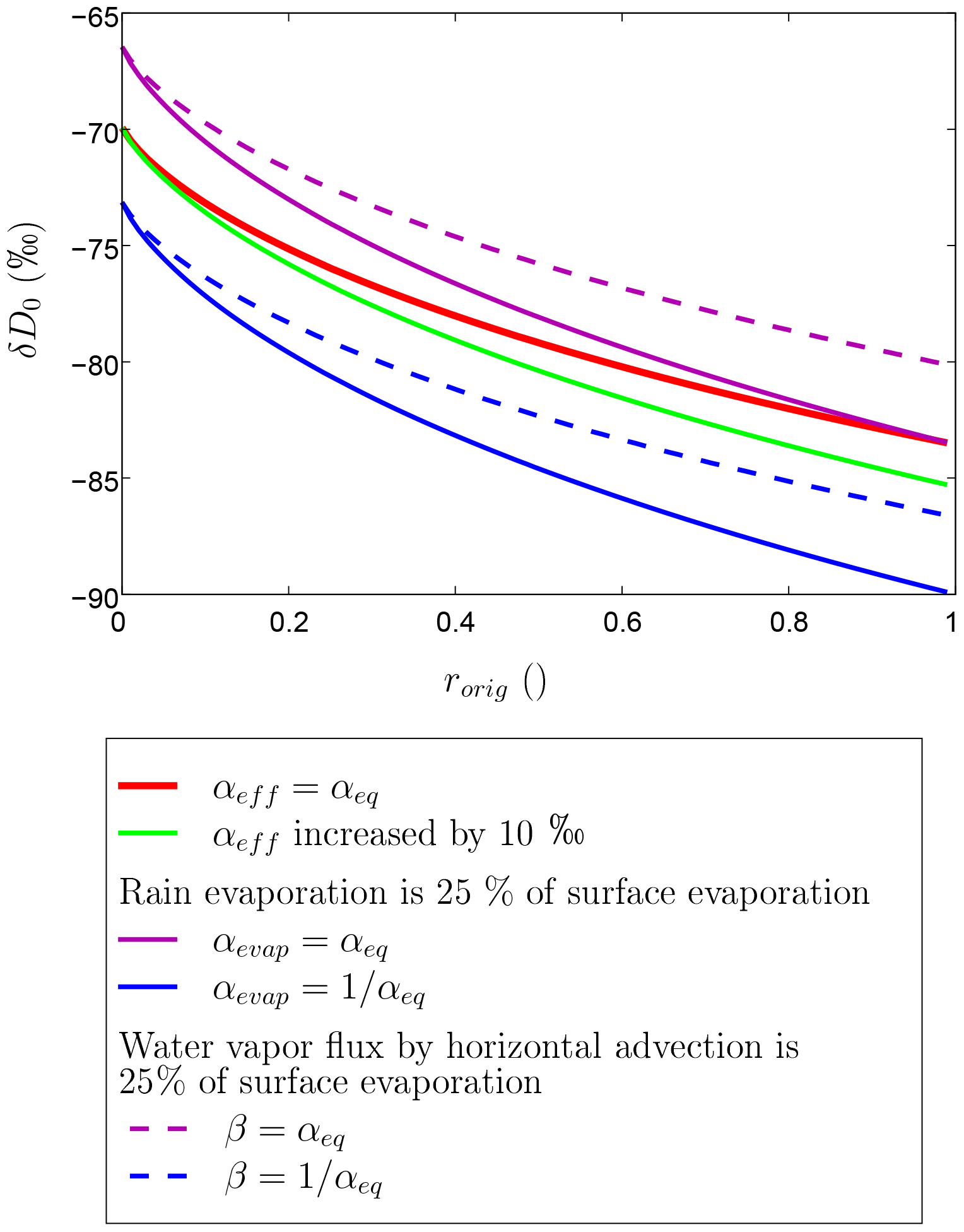
Figure 3δD0 as a function of rorig according to Eq. (9), with αeff=αeq as an example (red). For this illustrative purpose, we assume SST = 30 ∘C, h0=0.8, δDoce=0 ‰, and . The sensitivity to the effective fractionation factor αeff (green) is shown. If rain evaporation is 25 % of surface evaporation (η=0.25), the solid pink and blue curves show the sensitivity to the effective fractionation factor αevap. If the incoming water vapor by horizontal advection is 25 % of surface evaporation (ϕ=0.25), the dashed pink and blue curves show the sensitivity to the isotopic gradient quantified by β.

Figure 4Idealized q−δD diagrams showing how the SCL water vapor δD is set, for the case where the tropospheric δD profile follows Rayleigh distillation (a) or a mixing line (b). For this illustrative purpose, we assume SST = 30 ∘C, h0=0.8, δDoce=0 ‰, and . In (a), the red curve shows the Rayleigh profile starting from the SCL and the purple curve shows the mixing line connecting the air coming from above to the surface evaporation, in the case . The green curve shows the Rayleigh profile starting from the SCL and the blue curve shows the mixing line connecting the air coming from above to the surface evaporation, in the case . One can see that when rorig is lower, the mixing line is more curved, leading to more enriched values. In (b), the purple curve joins the SCL air and the air at all altitudes above the SCL. One can see that different values for rorig can lead to the same value of δD in the SCL.
3.1 LMDZ simulations
We use an isotope-enabled general circulation model (GCM) as a laboratory to test our hypotheses and investigate what controls the isotopic composition. We use the LMDZ5A version of LMDZ (Laboratoire de Météorologie Dynamique Zoom), which is the atmospheric component of the IPSL–CM5A coupled model (Dufresne et al., 2012) that took part in CMIP5 (Coupled Model Intercomparison Project; Taylor et al., 2012). This version is very close to LMDZ4 (Hourdin et al., 2006). Water isotopes are implemented the same way as in the predecessor LMDZ4 (Risi et al., 2010c). We use 4 years (2009–2012) of a simulation of the AMIP (Atmospheric Model Intercomparison Project) (Gates, 1992) that was initialized in 1977. The winds are nudged towards ERA-40 reanalyses (Uppala et al., 2005) to ensure a more realistic simulation. Such a simulation has already been described and extensively validated for isotopic variables in both precipitation and water vapor (Risi et al., 2010c, 2012a). The ocean surface water δDoce is assumed constant and set to 4 ‰. The resolution is 2.5∘ in latitude by 3.75∘ in longitude, with 39 vertical levels. Over the ocean, the first layer extends up to 64 m, and a typical SCL extending up to 600 m is resolved by six layers. Around 2500 m, a typical altitude for the inversion for trade-wind cumulus clouds, the resolution is about 500 m.
For our calculations, we only use tropical grid boxes (30∘ S–30∘ N) over tropical oceans (>80 % ocean fraction in the grid box). In addition, to avoid numerical problems when estimating the effect of horizontal advection and rain evaporation, only grid boxes and days where E>0.5 mm d−1 are considered. This represents 99.7 % of all tropical oceanic grid boxes.
Specific diagnostics for horizontal advection and rain evaporation are detailed in Appendix B and C.
3.2 STRASSE observations
We also apply our theoretical framework to observations during the STRASSE (Sub-Tropical Atlantic Surface Salinity Experiment) cruise that took place in the northern subtropical ocean in August and September 2012 (Benetti et al., 2014). This campaign accumulates several advantages that are important for our analysis: (1) continuous δD0 measurements in the surface water vapor (17 m) at a high temporal frequency during 1 month (Benetti et al., 2014, 2015, 2017b), (2) associated surface meteorological measurements, including SST and h0, (3) 22 radio soundings relatively well distributed over the campaign period and providing vertical profiles of altitude, temperature, relative humidity and pressure, (4) ocean surface water δDoce measurements (Benetti et al., 2017a), (5) a variety of conditions ranging from quiescent weather to convective conditions, (6) on many vertical profiles, a well defined temperature inversion allows to calculate the inversion altitude.
We use δD0 measurements on a 15 min time step. The measurements in ocean water were interpolated on the same time steps using a Gaussian filter with a width of 3 d. The radio-soundings are used together with all water vapor isotopic measurements that are within 30 min of the radio-sounding launch. Only profiles during the ascending phase of the balloon are considered because the descent phase is often located far away from the initial launch point (McGrath et al., 2006; Seidel et al., 2011).
3.3 Estimating the altitude from which the air originates
Here we explain how zorig is estimated based on LMDZ outputs. First, we assume that the q and δD at 500 hPa (qf, δDf) belong to a Rayleigh distillation line starting from the surface with effective fractionation αeff:
In a real field campaign, this assumption means that we do not need to measure the full vertical profile of δD, but only δDf at a given free-tropospheric altitude (e.g., 500 hPa).
We checked that results are similar when defining the end member at 400 hPa rather than 500 hPa. However, the end member should be defined above 500 hPa to ensure that it is well above boundary layer processes. If the end member is defined below 500 hPa (e.g., 600 hPa), there are a few cases where q increases with altitude (qf>q0) due to horizontal advection or convective detrainment from nearby moister regions; meanwhile, δD decreases monotonically, leading to unrealistic values for αeff.
Second, rorig is estimated based on Eq. (9), using αeff, αeq, αK , δDoce, h0, and δD0 simulated by LMDZ.
Third, the altitude zorig is estimated from rorig. Using the q vertical profile, we find zorig so that (Fig. 5, red).
When estimating zorig from observations, we follow the same methodology except that in absence of measurements for qf and δDf we assume a constant αeff=1.07 based on LMDZ simulation and that αeq, αK , δDoce, h0, and δD0 come from surface observations.
Note that rorig and zorig are not direct diagnostics from the simulation, but rather a posteriori estimates to match the simulated δD0. Therefore, if assumptions underlying Eq. (9) are violated, then the estimate of rorig, and subsequently zorig, will be biased. The estimate of rorig encapsulates the effect of mixing processes, but also all other processes that have been neglected in our theoretical framework, such as temporal variations in SCL depth, q0, or δD0 or vertical variations in q0 or δD0 within the SCL.
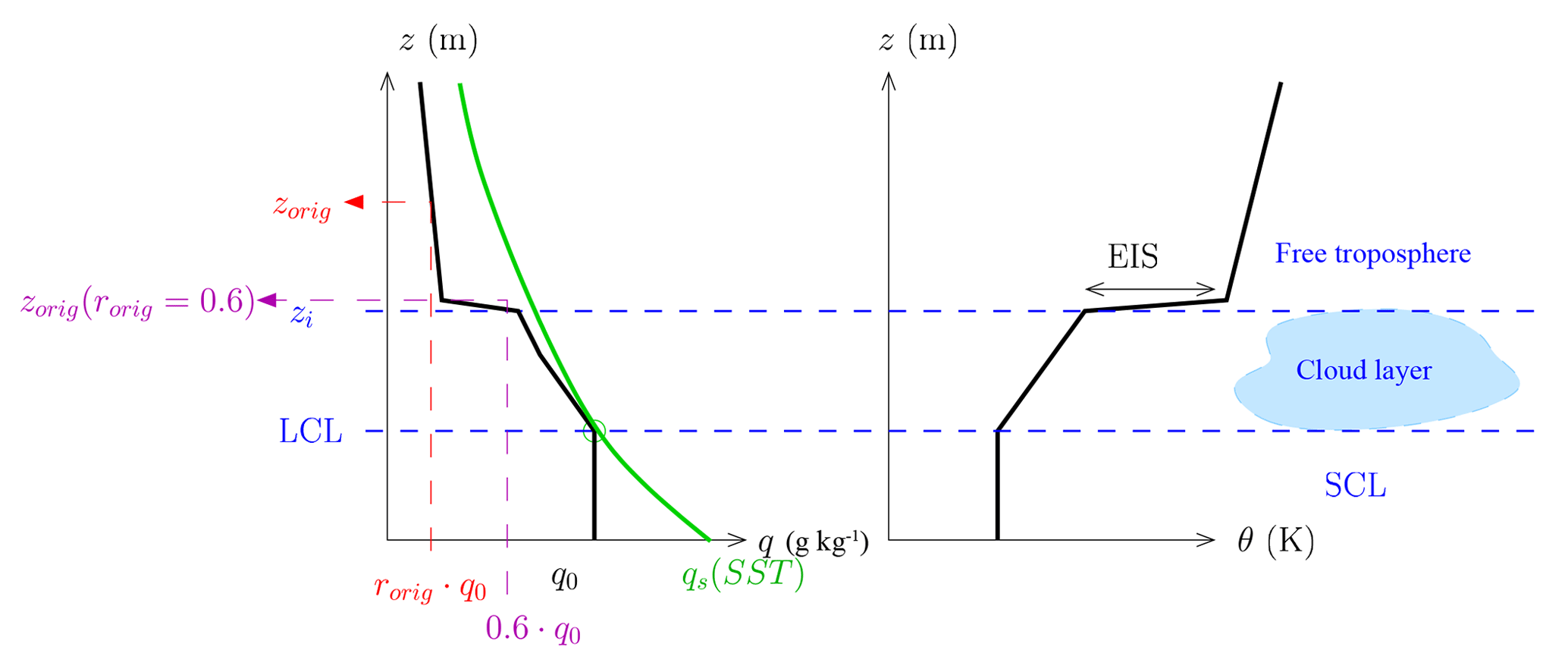
Figure 5Schematics illustrating the typical structure of tropical marine boundary layers. The sub-cloud layer (SCL) extends from the surface to the lifting condensation level (LCL) and the cloud layer extends from the LCL to the inversion (zi). EIS stands for the estimated inversion strength. Left: shape of the vertical profile in q (black) and qs (green). Right: shape of the vertical profile in potential temperature θ, inspired by Wood and Bretherton (2006). The LCL, zorig , , and zi altitudes defined in Sect. 3.4 are indicated.
3.4 Boundary layer structure diagnostics
Figure 5 illustrates the structure of a typical tropical marine boundary layer covered by stratocumulus or cumulus clouds (Betts and Ridgway, 1989; Wood, 2012; Wood and Bretherton, 2004; Neggers et al., 2006; Stevens, 2006). The cloud base corresponds to the lifting condensation level (LCL). Below is the well mixed SCL. Above is the cloud layer, topped by a temperature inversion. Above the inversion is the FT.
The LCL is calculated as the altitude at which the specific humidity near the surface equals the specific humidity at saturation of a parcel that is lifted following a dry adiabat (Fig. 5).
The temperature inversion is an abrupt increase in temperature that caps the boundary layer. Therefore, a method to automatically estimate its altitude zi is to detect a maximum in the vertical gradient of potential temperature (Stull, 1988; Oke, 1988; Sorbjan, 1989; Garratt, 1994; Siebert et al., 2000). This method is sensitive to the resolution of vertical profiles (Siebert et al., 2000; Seidel et al., 2010). Therefore, we adapted this method in order to yield zi values that best agree with what we would estimate from visual inspection of individual temperature profiles. In LMDZ, we calculate zi as the first level at which the vertical potential temperature gradient exceeds 3 times the moist-adiabatic lapse rate. In observations, we calculate zi as the first level at which the vertical potential temperature gradient exceeds 5 times the moist-adiabatic lapse rate because radio-soundings are noisier than simulated profiles.
Finally, we calculate zorig(rorig=0.6), which is the zorig altitude if rorig is set to 0.6. This usually coincides with the altitude of strong humidity decrease near the inversion (Fig. 5).
3.5 Averages and composites
All calculations are performed on daily values for LMDZ and on 15 min values for observations.
For LMDZ, when analyzing spatial and seasonal variability, seasonal averages are calculated at each grid box over tropical oceans by averaging all days of all years that belong to each season. Seasons are defined as boreal winter (December–January–February), spring (March–April–May), summer (June–July–August), and fall (September–October–November). For illustration purpose, all maps are plotted for boreal winter. Standard deviations are also calculated among all days of all years for each season.
The type of clouds and mixing processes depends strongly on the large-scale velocity at 500 hPa (ω500, map shown in Fig. 6a), with shallow clouds in subsiding regions and deeper clouds in ascending regions (Fig. 1). Therefore, it is convenient to plot variables as composites as a function of ω500 (Bony et al., 2004). To make such plots, we divide the ω500 range from −30 to 50 hPa d−1 into intervals of 5 hPa d−1. In each given interval, we average all seasonal-mean values at all locations over tropical oceans for which seasonal-mean ω500 belongs to this interval (e.g., Fig. 8a will be an example). Note that such composites are carried out on seasonal-mean ω500 because cloud processes and their associated diabatic heating are tied to the large-scale circulation through energetic constraints (Yanai et al., 1973; Emanuel et al., 1994) that are best valid at longer timescales, otherwise, the energy storage term may become significant (e.g., Masunaga and Sumi, 2017). This is why ω500 is generally averaged over a month or longer (e.g., Bony et al., 1997; Williams et al., 2003; Bony et al., 2004; Wyant et al., 2006; Bony et al., 2013). In addition, we primarily focus on understanding the seasonal and spatial distribution of δD0.
The cloud cover strongly correlates with the inversion strength, which can be quantified by the estimated inversion strength (EIS; Wood and Bretherton, 2006) (map shown in Fig. 6b) as a measure of inversion strength. We thus also plot variables as composites as a function of EIS. To make such plots, we divide the EIS range from −1 to 9 K into intervals of 0.5 K. In each given interval, we average all seasonal-mean values at all locations over tropical oceans for which seasonal-mean EIS belongs to this interval (e.g., Fig. 8b will be an example). Using seasonal-mean values is consistent with Wood and Bretherton (2006) and with the better link at longer timescales between cloud processes and the large-scale dynamical regime.
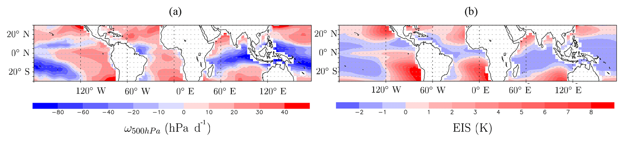
Figure 6Maps of winter-mean ω500 (a) and EIS (b) simulated by LMDZ.
3.6 Decomposition method for δD0
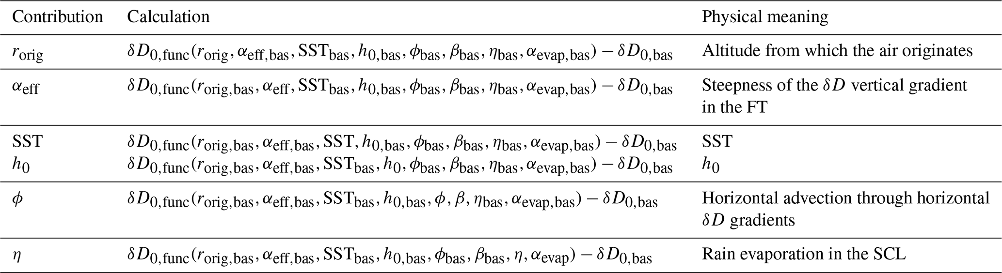
To understand what controls the δD0 spatiotemporal variations, δD0 is decomposed into four contributions based on Eq. (8). First, we define , , SSTbas=25 ∘C, , ϕbas=0, ηbas=0, βbas=1, and as a basic state. We call the function giving δD0 as a function of rorig, αeff, SST, h0, ϕ, β, η, and αevap following Eq. (8), and , αeff,bas, SSTbas, h0,bas, ϕbas, βbas, ηbas, αevap,bas). The relative contribution of rorig to δD0 is estimated as δD0,func (rorig, αeff,bas, SSTbas, h0,bas, ϕbas, βbas, ηbas, . Similarly, the contributions of αeff, SST, h0, ϕ, and η to δD0 are estimated as detailed in Table 1. All the contributions have the same units as δD0 (‰). The sum of these components yields a quantity that is very close to the simulated δD0, which confirms the validity of this linear decomposition. These components and their sum can be plotted as maps: Fig. 7 provides an example.
The relative contributions of each of these components to the δD variability are quantified by performing a linear regression of each of the components as a function of δD0. If the correlation coefficient is significant for a given factor, then the slope quantifies the contribution of this factor to the variability of δD0. The sum of all contributions may not always be 1 due to nonlinearity. Such a method has already been applied in previous studies (e.g., Risi et al., 2010b; Oueslati et al., 2016). The contributions to the seasonal spatial variability of δD0 can be quantified by performing the regression among all locations and seasons. The contributions to the daily variability of δD0 can be quantified by performing the regression among all days of a given season at a given location.
Table 1Equations to calculate the relative contributions of rorig, αeff, SST, h0, ϕ, and η to δD0 and the physical meaning of these contributions.
3.7 Decomposition method for rorig
To understand what controls rorig, a similar method as for the decomposition of δD0 can be applied. We can write rorig as
where is the temperature at altitude zorig, is the tropical-ocean-mean temperature profiles, h(zorig) and P(zorig) are the relative humidity and pressure at zorig, and δT(zorig) is the temperature perturbation compared to . Therefore, the variability of rorig is decomposed into the effect of four factors: q0, zorig, h(zorig), and δT(zorig). In practice, rorig and zorig are calculated following Sect. 3.3, and then Eq. (11) is applied.
4.1 Decomposition of δD0 variability
The spatial variations in δD0 simulated by LMDZ (Fig. 7a) are characterized by depleted values near midlatitudes and in dry subsiding regions (e.g., off the coast of Peru and over other regions of oceanic upwelling) and regions of atmospheric deep convection (e.g., Maritime Continent). Consistently, δD0 values exhibit a maximum for weakly ascending or subsiding regions: δD0 decreases with increasing vertical velocity of both signs (Fig. 8a black); δD0 decreases as EIS increases reflecting more stable, subsiding conditions (Fig. 8b black). This pattern is consistent with previous studies (e.g., Good et al., 2015). For the first time, we propose a theoretical framework to interpret this pattern, decomposing it into six contributions: rorig, αeff, SST, h0, rain evaporation, and horizontal advection effects (Sect. 3.6). We check that the reconstructed δD0 from the sum of its four contributions is very similar to the simulated δD0 (Figs. 7b, 8 dashed black).
In ascending regions, the main contribution explaining the more depleted δD0 in deep convective regions is that of αeff (Figs. 7d, 8a red). αeff is higher in more ascending regions (Fig. D1d). This means that the main factor depleting δD0 in deep convective regions is the fact that the mid-troposphere is more depleted. This leads to a steeper gradient (higher αeff), and thus a more efficient depletion by vertical mixing. This is consistent with deep convection depleting the water vapor most efficiently in the mid-troposphere (Bony et al., 2008). The second main contribution is that associated with rorig (Figs. 7c, 8a green). rorig is larger in deep convective regions (as explained in Sect. 4.2).
In subsidence regions, SST is the main factor controlling δD0 (Figs. 7e, 8a pink): as subsidence is stronger, or as EIS increases, SST is colder, leading to larger αeq and thus more depleted δD0. Another important factor is h0 (Figs. 7f, 8a purple): as subsidence is stronger, h0 is drier, leading to more depleted δD0. The contribution of rorig is also a significant contribution to the depletion of δD0 in the cold upwelling regions, for example off Peru or Namibia (Fig. 7c). The shallower boundary layer there is associated with higher rorig.
The contribution of rain evaporation on δD0 is minor compared to other contributions, except in the deepest convective regions (Fig. 7g). Rain evaporation is a slightly depleting effect in regions of strong deep convection and a slightly enriching effect in regions of moderate deep convection. When the fraction of raindrops that evaporate is small, isotopic fractionation favors evaporation of the lighter isotopologues. Therefore in convective, moist regions, rain evaporation has a depleting effect on the SCL (Worden et al., 2007). In contrast, in drier regions, rain evaporates almost totally. The evaporation flux thus has almost the same composition as the initial rain, which is more enriched than the water vapor.
The contribution of horizontal advection to δD0 is significant only where isotopic gradients are the largest (Fig. C1h). Horizontal advection has slightly enriching in deep convective regions and depleting in coastal regions (e.g., off the coasts of California, Peru, Mauritania, Namibia, India, and Australia). For example, the Saharan layer off the northwestern African coast leads to a strong effect of horizontal advection (Lacour et al., 2017a).
From a quantitative point of view, we can decompose the δD0 seasonal spatial variations into these different effects (Sect. 3.6). In regions of large-scale ascent, αeff is the main factor explaining the δD0 seasonal spatial variations (33 %), followed by rain evaporation (20 %) and rorig (19 %; Table 2). In regions of large-scale descent, SST is the main factor explaining the seasonal spatial variations (54 %), followed by rorig (29 %), h0 (13 %), and αeff (10 %) (Table 2). Note that the contribution of rorig would be similar if we neglect rain evaporation and horizontal advection effects (Table 2).
The decomposition method can also be applied to decompose the δD0 variability at the daily timescale at each location and for each season (Table 3). On average, in ascending regions, rorig is the main factor (52 %), followed by rain evaporation (48 %) and αeff (35 %). In subsiding regions, the effect of SST is muted due to its slow variability, and rorig (82 %) becomes the main factor.
Overall, the results highlight the importance of rorig as one of the main factors controlling the spatiotemporal variability of δD0.
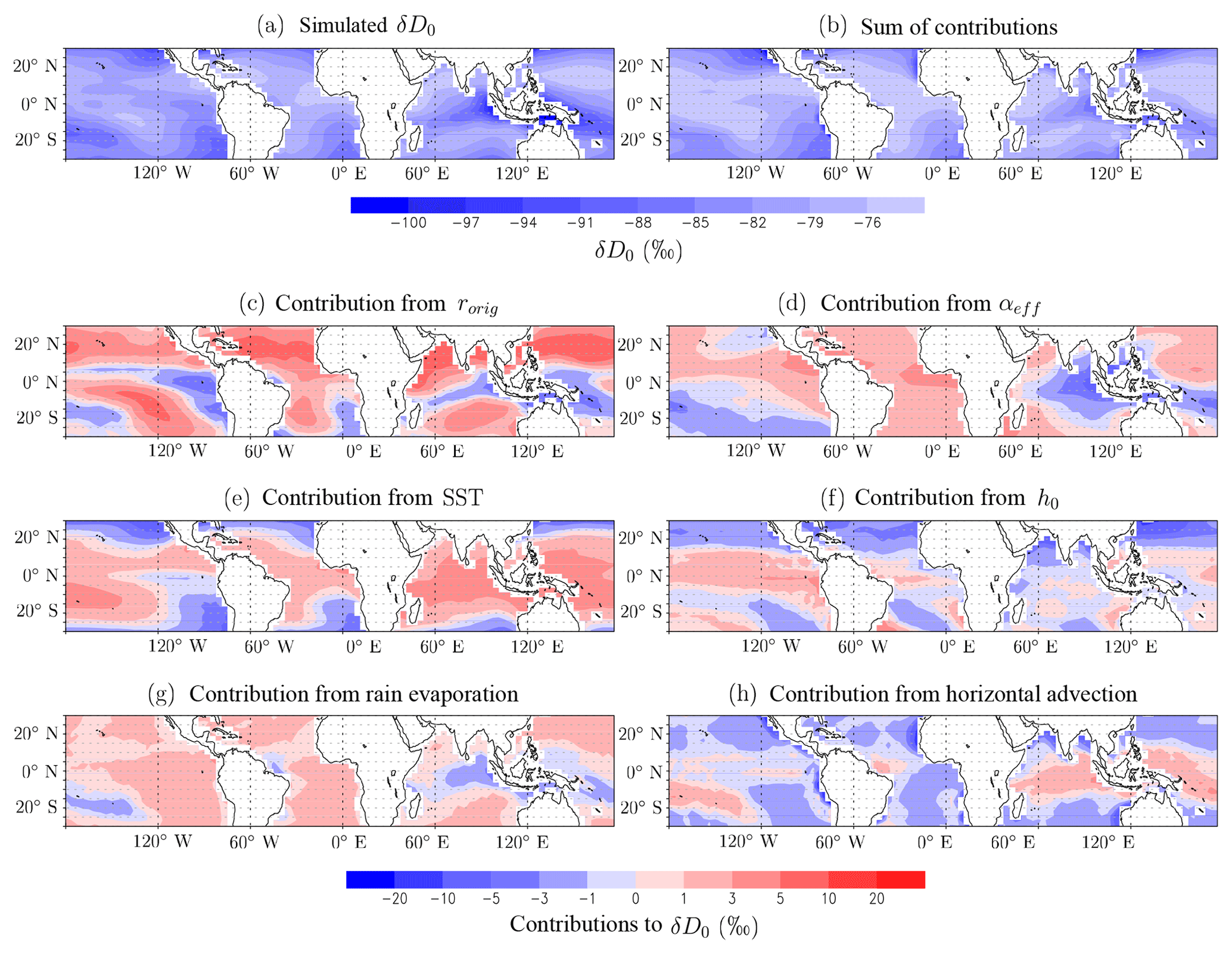
Figure 7(a) Map of winter-mean δD0 simulated by LMDZ. (b) Map of winter-mean δD0 reconstructed as the sum of the four contributions. Tropical-mean δD0 was added to compare with (a) on the same color scale. (c) Map of the contribution of rorig on winter-mean δD0 calculated from Eq. (9) (see Sect. 3.6). (d) Same as (b) but varies for αeff. (e) Same as (b) but for SST. (f) Same as (b) but for h0.
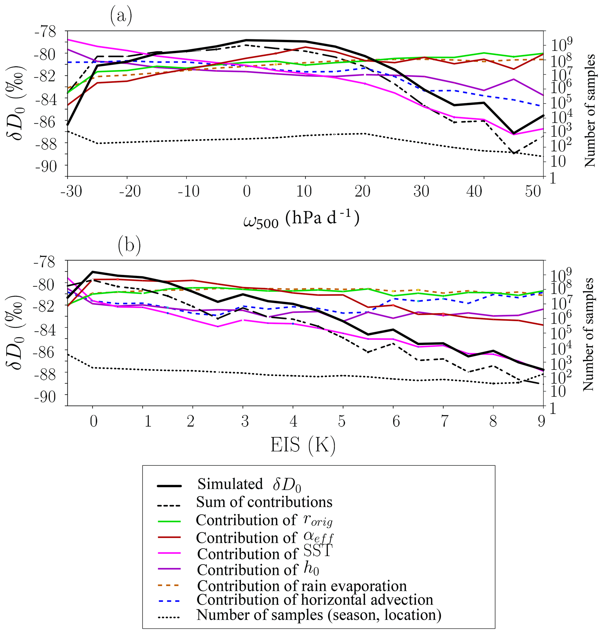
Figure 8Composites as a function of ω500 (a) and of EIS (b) of the seasonal averages of δD0 simulated by LMDZ over all tropical ocean locations (black). Same for the sum of the contributions (black dashed and for each individual contribution to δD0: rorig varies (green), αeff (dark red), SST (pink), h0 (purple), rain evaporation (dashed brown), and horizontal advection (dashed blue). The tropical mean δD0 was added to each contribution to plot on the same scale as simulated δD0. The number of samples in each bin is indicated on a logarithmic scale on the right-hand side (dotted black line).
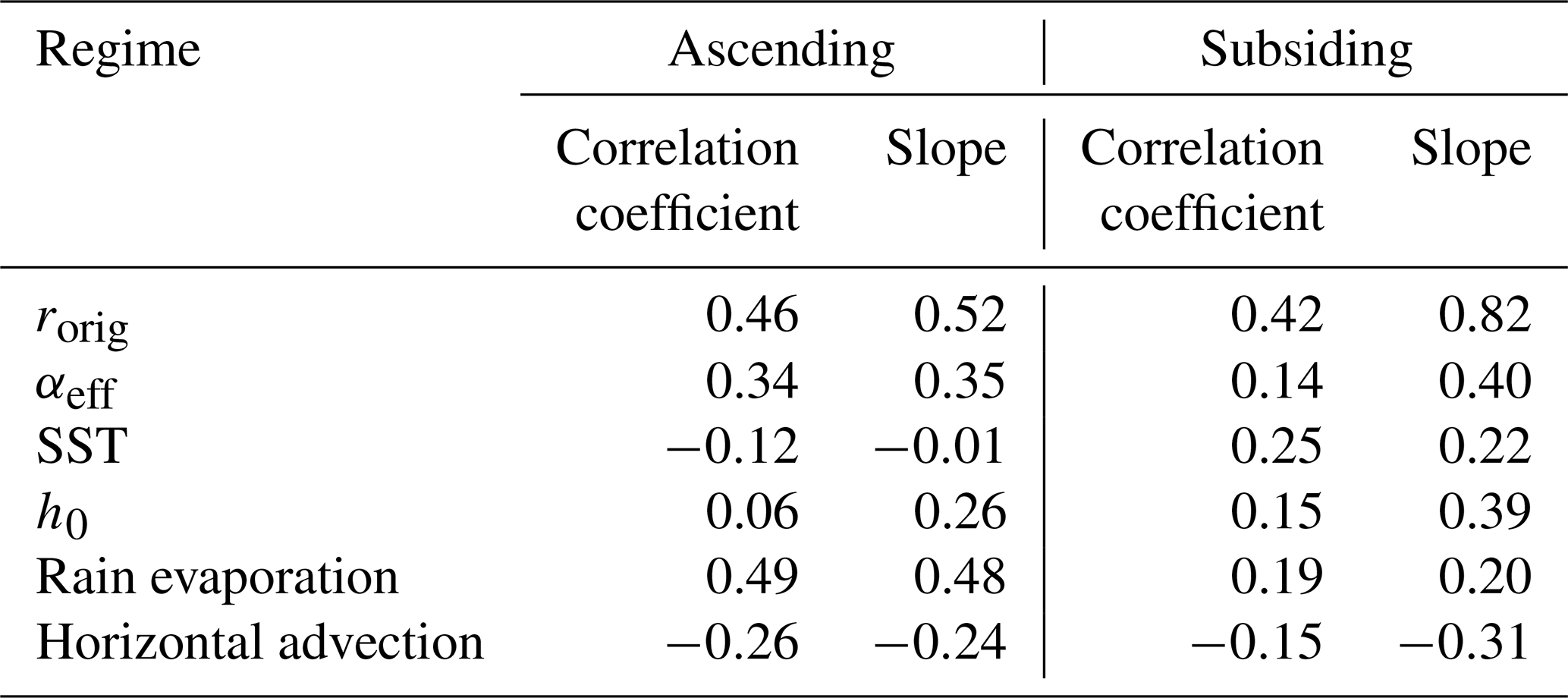
Table 2Decomposition of the spatial and seasonal variation in δD0 into its six contributions: effect of rorig, αeff, SST, h0, rain evaporation, and horizontal advection. For each contribution, we show the correlation coefficient of the linear regression of the contribution as a function of δD0. The analysis is performed separately for ascending and subsiding regimes. All seasons and locations over tropical oceans (30∘ N–30∘ S, ocean fraction >80 %, surface evaporation >0.5 mm d−1) are considered. The threshold for the correlation coefficient to be statistically significant at 99 % is 0.15 or lower in all cases. We write correlation coefficient and slope values between brackets when they are not significant at 99 %.
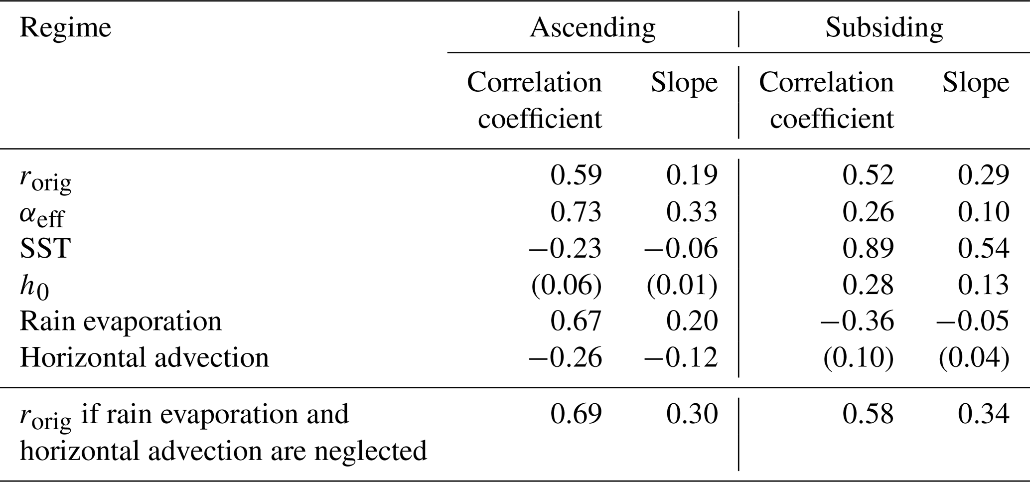
Table 3As in Table 4 but at the daily scale. The correlation coefficients and slopes are averaged over all seasons and locations over tropical oceans (30∘ N–30∘ S, ocean fraction >80 %), separately for ascending and subsiding regimes.
4.2 Decomposition of rorig variability
Given the importance of rorig in controlling the δD0 variations, we now decompose rorig into its four contributions: q0, zorig, horig, and δTorig (Sect. 3.6). Spatially, rorig is maximum in regions of strong large-scale ascent (Fig. 10a) such as the Maritime Continent (Fig. 9a) and in very stable regions (Fig. 10b) such as upwelling regions (Fig. 10a). We check that the reconstructed rorig from the sum of its four contributions is very similar to the simulated rorig (Figs. 9b, 10 dashed black).
In regions of strong large-scale ascent, rorig is larger mainly because horig is larger (Figs. 9e, 10a pink). This is because the moister the FT, the higher the contribution of vapor coming from above to the vapor of the SCL, and thus the higher rorig and the more depleted δD0. This mechanism through which a moister FT leads to a more depleted δD0 is consistent with that argued in B15. zorig damps this effect: when convection is stronger and the FT moister, convection is also deeper, so the air originates from higher altitudes where the air is drier.
In very stable regions, rorig is larger because q0 is larger (Figs. 9c, 10b green), consistent with the drier conditions in these regions of large-scale descent. Note that this effect can be seen only in the most stable regions, but when considering all subsiding regions, the contribution is small (Table 2). rorig is also larger because zorig is lower in altitude (Figs. 9d, 10b red). As EIS increases, the boundary layers are shallower, the air comes from lower in altitude, rorig is higher, and thus δD0 is more depleted. This mechanism was not considered in B15 but our decomposition shows that it is a key mechanism driving rorig and thus δD0 variations in stable regions.
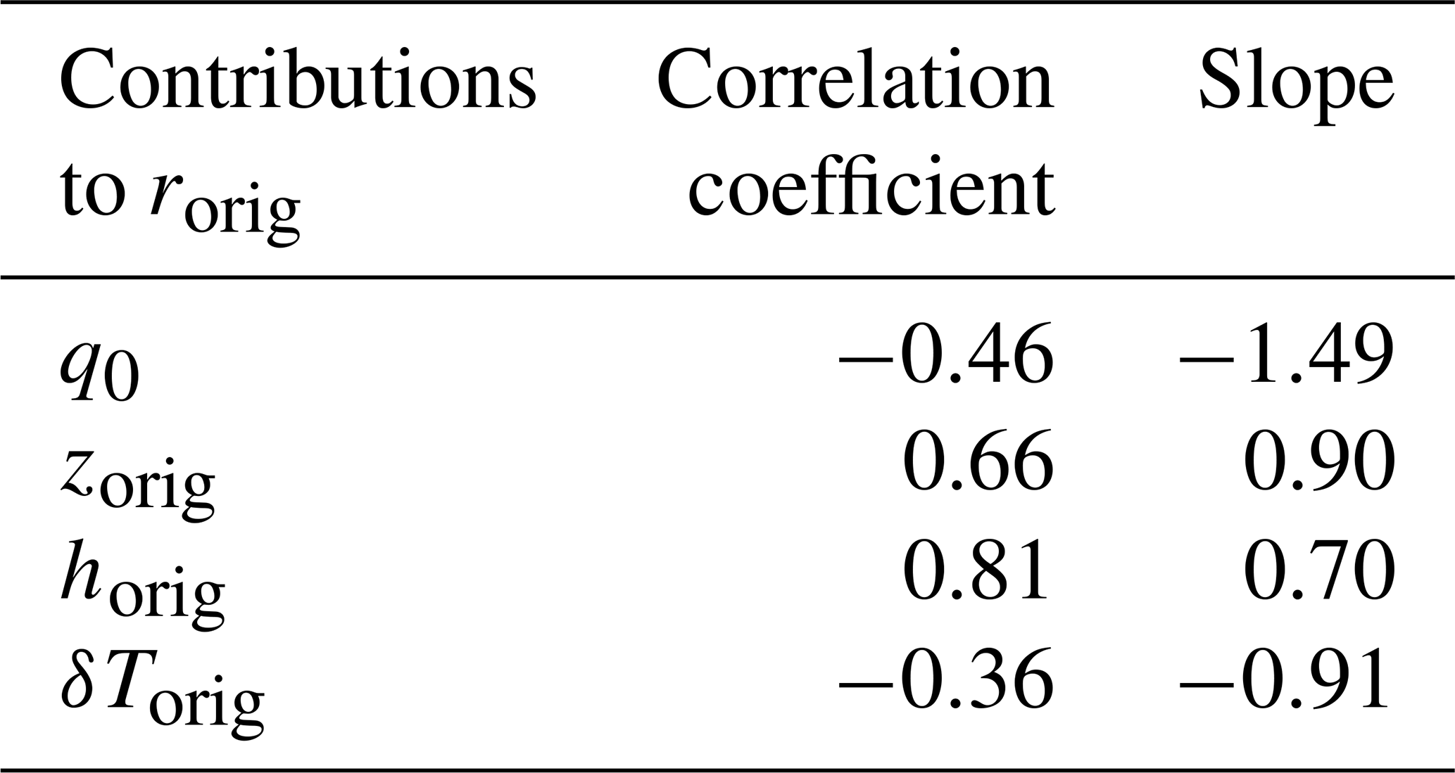
Quantitatively, in ascending regions, the main factor controlling the seasonal spatial variations in rorig is horig (182 %), dampened by zorig (−67 %) (Table 4). In descending regions, the main factor is also horig (96 %), followed by zorig (41 %) (Table 4). At the daily scale, the same two factors dominate the variability of rorig: horig and zorig contribute to 78 % and 39 % of rorig variations on average over ascending regions and to 118 % and 39 % on average over descending regions (Table 5).
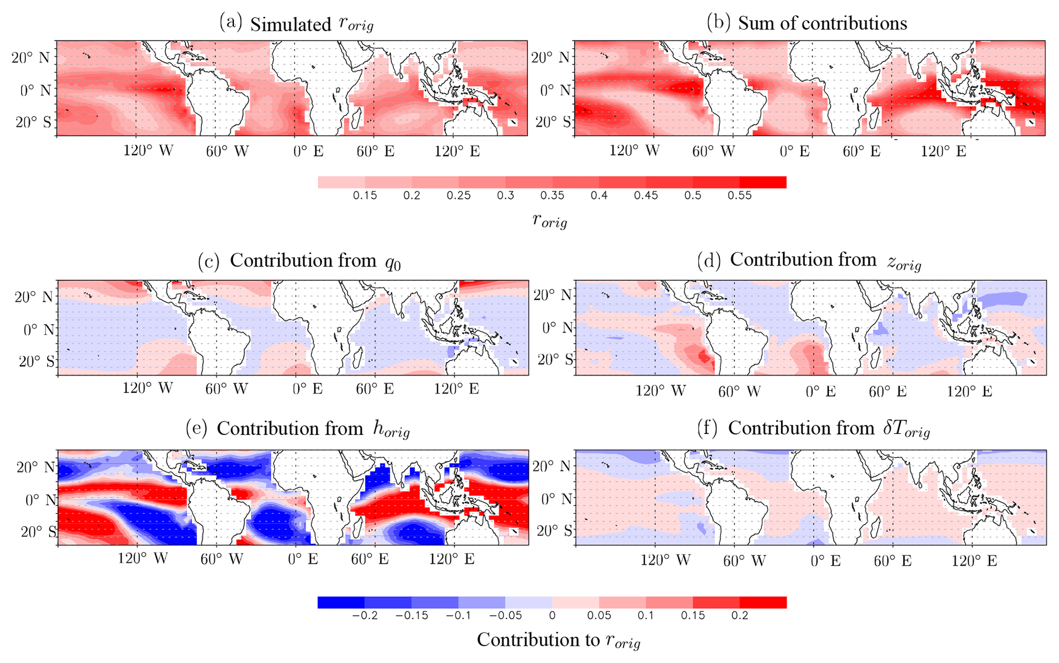
Figure 9(a) Map of winter-mean rorig simulated by LMDZ. (b) Map of winter-mean rorig reconstructed as the sum of the four contributions. Tropical-mean rorig was added to compare with (a) with the same color scale. (c) Map of winter-mean rorig calculated from Eq. (11) if only q0 varies (see Sect. 3.6). (d) Same as (b) but if only zorig varies. (e) Same as (b) but if only h(zorig) varies. (f) Same as (b) but if only δTorig varies.
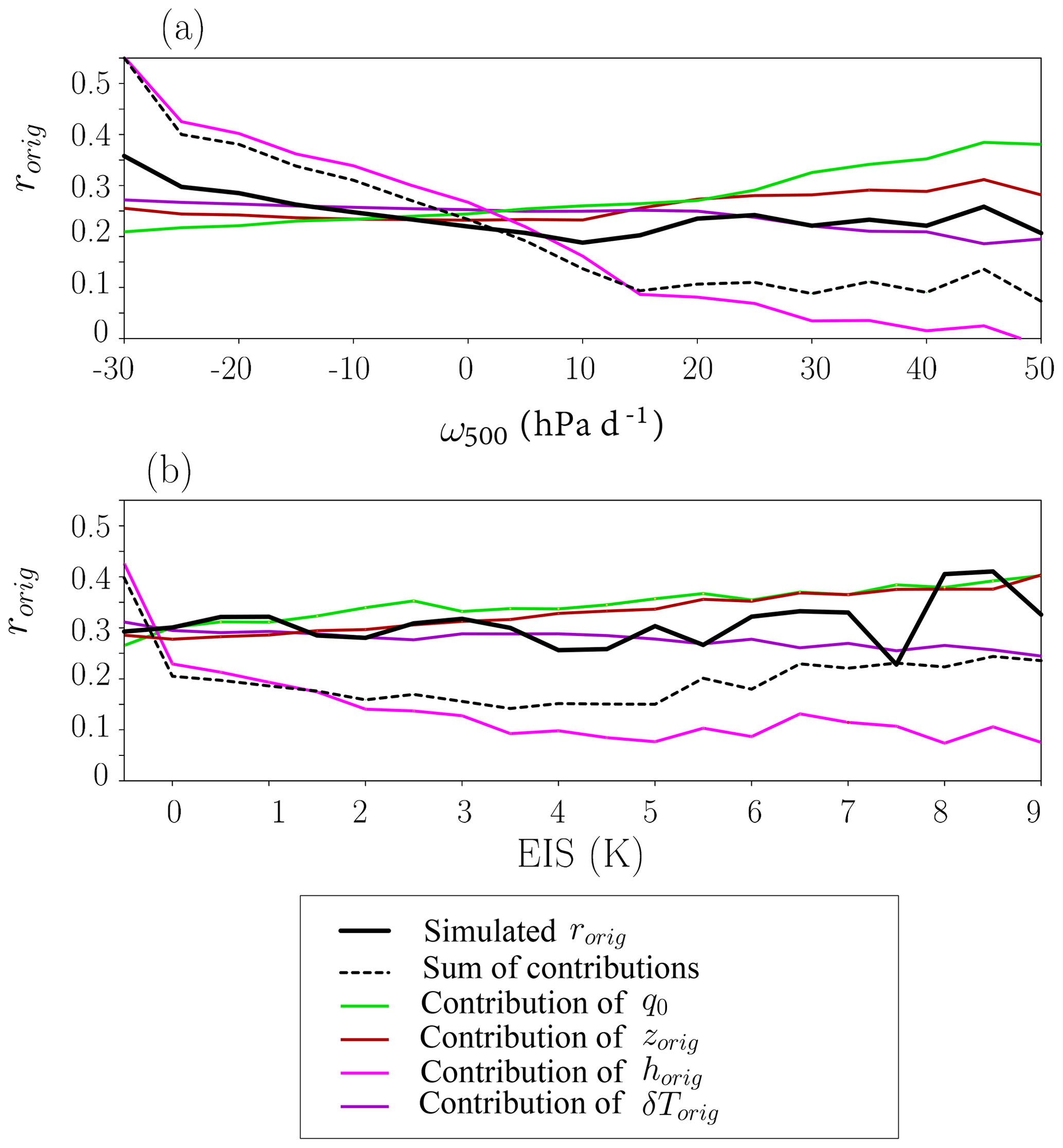
Figure 10Composites as a function of ω500 (a) and of EIS (b) of the seasonal averages of rorig simulated by LMDZ over all tropical ocean locations (black). Same for the sum of the contributions (black dashed) and for each individual contribution to rorig:q0 varies (green), zorig (dark red), h(zorig) (pink), and δTorig (purple). The number of samples in each bin is indicated on a logarithmic scale on the right-hand side as bars.
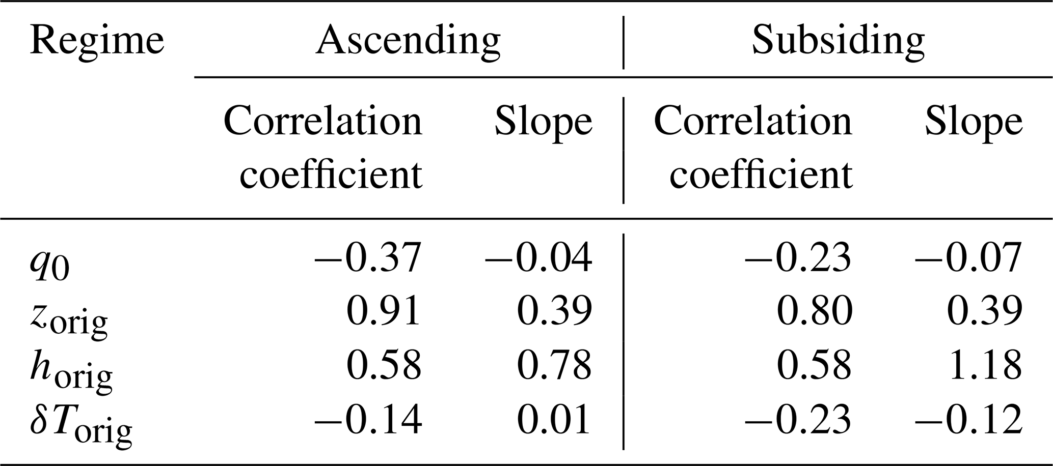
Table 4Decomposition of the spatial-seasonal variation in rorig into its four contributions: effect of q0, zorig, horig, and δTorig variations. For each contribution, we show the correlation coefficient of the linear regression of the contribution as a function of rorig. The analysis is performed separately for ascending and subsiding regimes. All seasons and locations over tropical oceans (30∘ N–30∘ S, ocean fraction >80 %) are considered. The threshold for the correlation coefficient to be statistically significant is 0.15 or lower in all cases. We write correlation coefficient and slope values between brackets when they are not significant at 99 %.
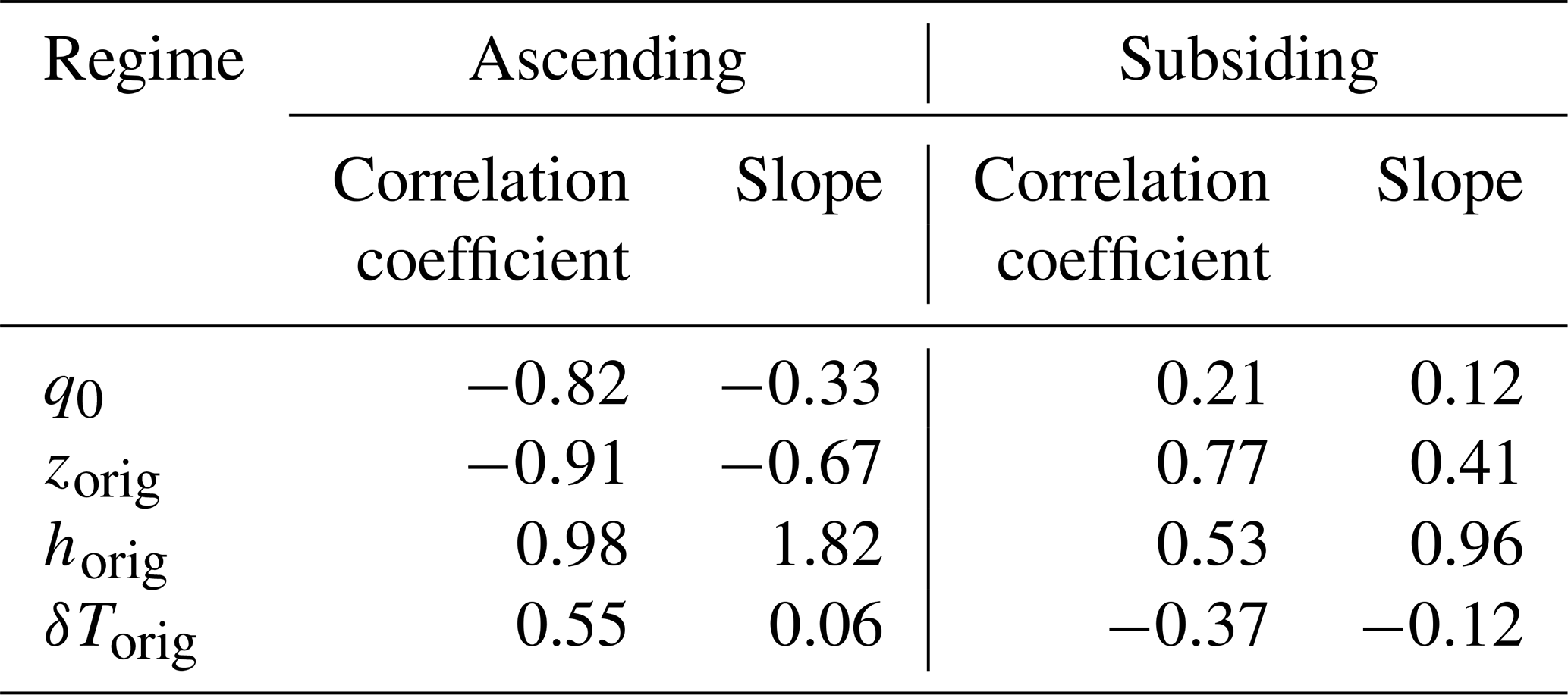
Table 5As in Table 4 but at the daily scale. The correlation coefficients and slopes are averaged over all seasons and locations over tropical oceans (30∘ N–30∘ S, ocean fraction >80 %), separately for ascending and subsiding regimes.
4.3 Estimating altitude zorig
Estimated altitude zorig is at a minimum in dry subsiding regions, especially in upwelling regions (Figs. 11a, and 12), corresponding to regions with the strongest inversion (Fig. 11). This contributes to the depleted δD0 in these regions.
As explained in Sect. 3.3, our estimate of zorig may be artificially biased due to the neglect of some processes in our theoretical framework. Ideally, to check whether zorig really physically represents the altitude from which the air originates, additional model experiments where water vapor from different levels are tagged (Risi et al., 2010b) would be needed. While we leave this for future work, we check whether zorig estimates are consistent with what we expect based on what we know about mixing processes in the marine boundary layers. We expect that in stratocumulus regions, air originates from a very shallow (a few tens of meters) layer above the inversion, whereas the mixing processes may be more diverse, and possibly deeper in the FT, as the boundary layer deepens (Fig. 1).
To check whether estimated zorig is consistent with this picture, we compare zorig to zorig(rorig=0.6) (zorig that we would estimate is rorig was set constant to 0.6) and zi (Sect. 3.4), which are measures of the altitude of the humidity drop and temperature inversion, respectively. As expected from Fig. 1, they are minimum in dry upwelling regions, intermediate in trade-wind regions, and maximum values in convective regions (Figs. 11c–d, 12 green, blue). Therefore, the low zorig in upwelling regions reflects the low zi. Consistently, in subsiding regions, zorig correlates well with (correlation coefficient of 0.52, statistically significant beyond 99 %). If we focus on very stable regions only (EIS >7 K), zorig correlates well with both zorig(rorig=0.6) and zi (correlation coefficient of 0.58 and 0.52, respectively, statistically significant beyond 99 %). The altitude zorig is a few meters above the inversion in stratocumulus regions, and up to 1 km above the inversion in cumulus and deep convective regions (Fig. 12), consistent with our expectations from Fig. 1. This lends support to the fact that at least in subsiding regions, our isotope-based zorig estimate effectively reflects the origin of air coming from above.
In ascending regions, in contrast, zorig does not correlate significantly with zorig(rorig=0.6) or zi. This may indicate either that our zorig estimate is biased by neglected processes such as rain evaporation or that in deep convective regions the origin of FT air into the SCL is very diverse due to the variety of mixing processes (Fig. 1).

Figure 11(a) Map of winter-mean zorig estimated from δD0 simulated by LMDZ. (b) Same as (a) but zorig that we would estimate if rorig were constant set to 0.6, zorig(rorig=0.6). (c) Same as (a) but for zi simulated from LMDZ. Only days when EIS >2 K are considered, otherwise zi is difficult to estimate. (d) Same as (a) but for LCL simulated by LMDZ.
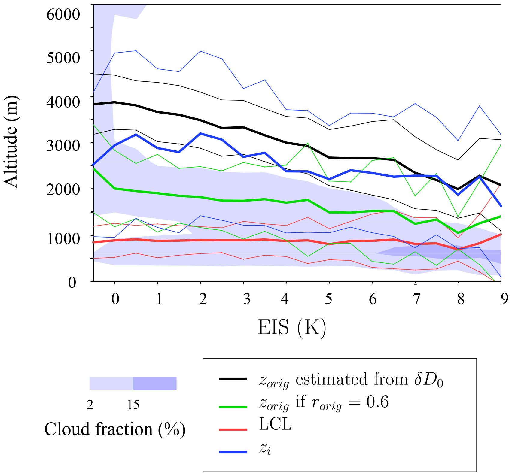
Figure 12Composites as a function of EIS of seasonal mean of zorig (black), zorig(rorig=0.6) (green), zi (blue), and LCL (red). The composite profiles of cloud cover are also shown, showing deep clouds when EIS is close to 0 and the shallowest clouds when EIS is largest.
To check whether our results obtained with LMDZ are realistic, we apply our methods to the measurements gathered during the STRASSE campaign. For simplicity and in absence of all necessary measurements, here we neglect the effects of rain evaporation and horizontal advection.
Throughout the cruise, δD0 shows a large variability, ranging from around −75 ‰ in quiescent conditions to −120 ‰ during the two convective conditions (Benetti et al., 2014) (Fig. 13a red). Variability in rorig is the major factor contributing to this variability (58 %) (Fig. 13a green, Table 6). This crucial importance of mixing processes is consistent with B15.
During the two convective events, the estimated rorig saturates at 1 (Fig. 13b). This proves that rorig estimated in these conditions is biased high because it encapsulates the effect of neglected processes, i.e., depletion by rain evaporation. Equation (9) is not valid in this case. In addition, at the scale of a few hours, the steady-state assumptions may be violated. Rain evaporation may strongly deplete the SCL before surface evaporation has the time to play its dampening role, hence the possibility of reaching very low δD0 that cannot be predicted even when considering rain evaporation (Appendix B).
During the rest of the cruise, the main factors controlling the rorig variability are zorig (90 %) and horig (70 %). The importance of FT humidity in controlling rorig was already highlighted in B15. However, in their paper, the variability in zorig was neglected, whereas it appears here as the main factor.
Through September, the cruise goes from a shallow boundary layer in early September to deeper boundary layers with higher inversions, before reaching the convective conditions (Fig. 13c). Consistently with this deepening boundary layer, the air originates from increasingly higher altitudes. Remarkably, there are 6 d when zorig coincides with zi with a root-mean-square error of 31 ‰ and correlation coefficient of 0.996 (Fig. 13c). This indicates that the air comes exactly from the inversion layer. When recalling that zorig and zi are estimated from completely independent observations, the coincidence is remarkable and lends support to the fact that on these days, our zorig estimate is physical. However, there remain 9 d when zorig is much higher than zi. This may reflect more penetrative downdrafts as we approach deeper convective regimes. But it may also be an artifact of our neglect of horizontal advection. For example, on these days which are characterized by lower h0, neglecting the advection of enriched water vapor from nearby regions with higher h0 could be misinterpreted as lower rorig and thus higher zorig.

Figure 13(a) Time series of δD0 observed during the STRASSE cruise, together with its four contributions. The δD of the surface ocean water is also plotted with the scale on the right. (b) Time series of rorig estimated from observations during the STRASSE campaign, together with its four contributions. (c) Times series of zorig, zorig(rorig=0.6), LCL, and zi estimated from the STRASSE observations.
Table 6Same as Table 2 but for the STRASSE observations. Linear regressions are calculated among 1977 data points.
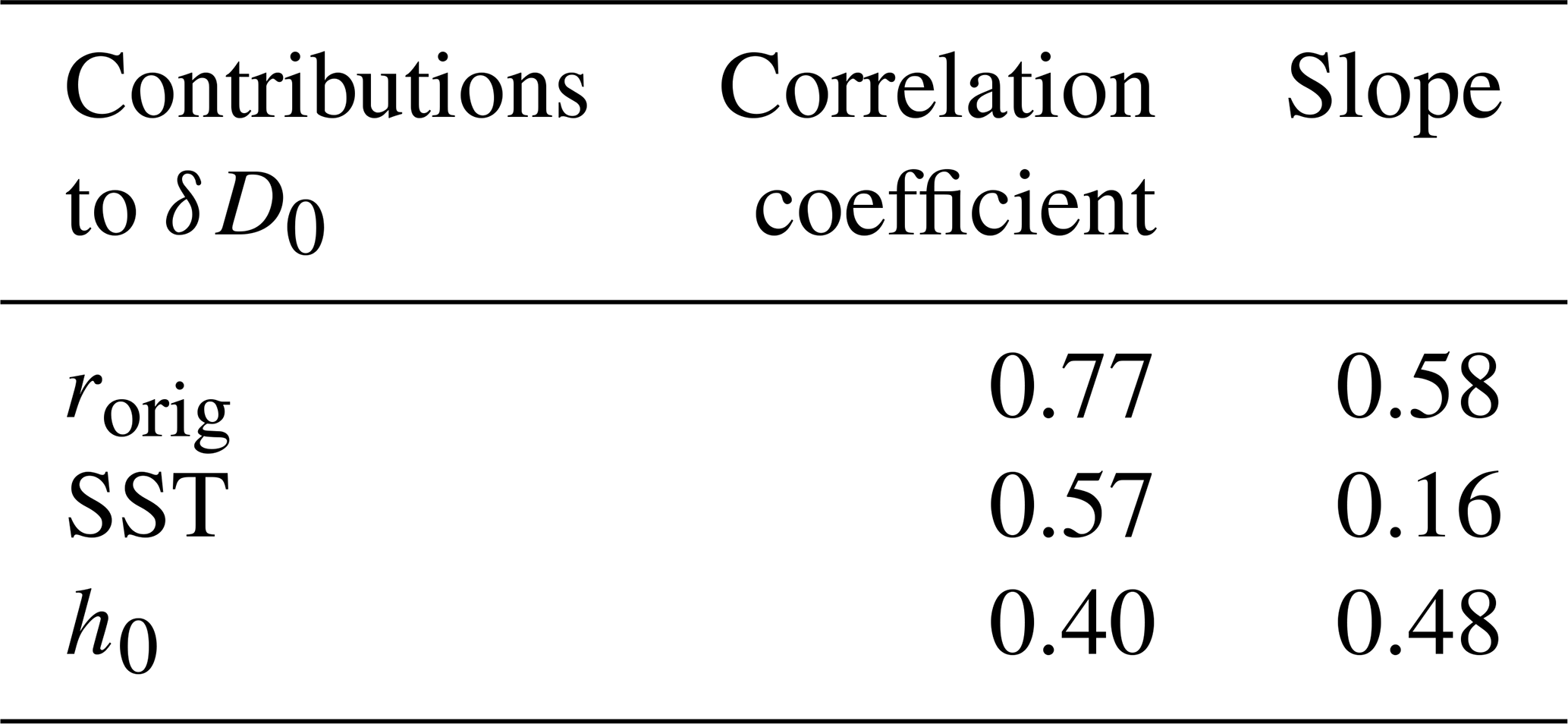
Table 7Same as Table 4 but for the STRASSE observations. Linear regressions are calculated among 55 data points, so that correlation coefficients above 0.35 are statistically significant at 99 %.
We have shown in the previous section that one of the main factors controlling δD0 at the seasonal spatial and daily scales is the proportion of the water vapor in the SCL that originates from above (rorig) and that one of the main factors controlling rorig is the altitude from which the air originates (zorig). In turn, could we use water vapor isotopic measurements to constrain zorig? This would open the door to discriminating between different mixing processes at play (Fig. 1). Since mixing processes are crucial to determine the sensitivity of cloud fraction to SST (Sherwood et al., 2014; Bretherton, 2015; Vial et al., 2016), such a prospect would allow us to improve our knowledge of cloud feedbacks, and hence of climate sensitivity.
With this in mind, we assess the errors associated with zorig estimates from δD0 measurements, and discuss whether they are small enough for zorig estimates to be useful. In stratocumulus clouds where the air is believed to originate from the first few tens of meters above cloud top (Faloona et al., 2005; Mellado, 2017), zorig estimates are not useful if the errors are larger than a few tens of meters, e.g., 20 m. In cumulus clouds where mixing processes are more diverse and possibly deeper (Fig. 1), zorig estimates may be useful if errors are of the order of 80 m.
Let us assume that we have a field campaign where we measure δD0, surface meteorological variables, temperature and humidity profiles (e.g., radio soundings), and a few δD profiles (e.g., by aircraft). This is what we can expect for example from the future EUREC4A (Elucidating the role of clouds-circulation coupling in climate) campaign to study trade-wind cumulus clouds (Bony et al., 2017). Below we quantify the effects of five sources of uncertainty on zorig estimates.
6.1 Measurement errors
The first source of uncertainty is measurement errors. We recalculate zorig assuming an error of 0.4 ‰ on δD0 (typical of what we can measure with in-situ laser instruments; Aemisegger et al., 2012; Benetti et al., 2014) and 1 ‰ on δDf (larger errors due to lower humidity and the increased complexity of measurements in altitude). The averaged errors on zorig and their standard deviations are plotted as a function of EIS in Fig. 14a. Whereas errors on δDf lead to errors on zorig of the order of 20 m (Fig. 14a, green), errors on δD0 lead to errors on zorig of the order of 80 m (Fig. 14a, red). Yet in stratocumulus, no one expects the air to originate from a higher altitude than 80 m above the inversion. Therefore, δD0 measurements would need to be more accurate than usual to be useful in stratocumulus regions, i.e., 0.1 ‰ to yield a 20 m precision on zorig. In trade-wind cumulus regions, the precision of 0.4 ‰ is enough for zorig to be useful.
6.2 Neglecting rain evaporation
The second source of uncertainty is associated with neglecting rain evaporation. This effect can be quantified in a model, but it is very difficult to quantify in nature because it is complicated and uncertain to measure η (Rosenfeld and Mintz, 1988), and it is even more complicated to measure or predict αevap. Rain evaporation can have a depleting or enriching effect depending on microphysical details that are too complex to be addressed here (Graf et al., 2019). Neglecting rain evaporation leads to an error of the order of 500 m in regions of low EIS and 250 m in regions of strong EIS (Fig. 14b, brown). In regions of stratocumulus regions, rain evaporation is a significant source of error in spite of the relatively small amount of precipitation available to evaporate. This is because total evaporation of the rain efficiently enriches the SCL and easily modifies δD0 by more than the 0.1 ‰ targeted precision explained above. However, it is possible that LMDZ overestimates this source of error in trade-wind cumulus and stratocumulus regions. LMDZ is one of the GCMs producing the strongest rain in stratocumulus regions (Zhang et al., 2013), and GCMs are known to trigger convection too often in trade-wind cumulus regions (Nuijens et al., 2015a, b).
6.3 Neglecting horizontal advection
The third source of uncertainty is associated with horizontal advection. In nature, ϕ can be estimated from meteorological analyses and β can be estimated from near-surface isotopic measurements at several locations (e.g., sounding arrays during typical field campaigns). In absence of these additional measurements, neglecting this effect leads to an error of the order of 800 m (Fig. 14b, purple). This limits the usefulness of zorig estimates for all cloud regimes.
6.4 Daily variability in the steepness of δD profiles
The fourth source of uncertainty arises from the daily variability in αeff (Appendix D2). Estimating αeff requires us to measure δDf at 500 hPa. Satellite measurements are available but are affected by random errors that are too large for our application (Worden et al., 2011, 2012; Lacour et al., 2015). Precise in situ measurements of water vapor δD in altitude are costly and difficult (Sodemann et al., 2017).
Let us assume that we have only one δDf value that represents the seasonal average at a given location. To estimate the resulting error on zorig, we re-estimate zorig every day and at each location using and . The error on zorig is calculated as . The averaged error and its standard deviation is plotted as a function of EIS in Fig. 14c (black). It is of the order of 400 m and rarely below 200 m. If we attempt to estimate αeff as the fractionation coefficient as a function of local temperature, errors would be even more dissuasive (Fig. 14c, blue).
Therefore, estimating zorig from daily δD0 measurements cannot be useful unless we measure δDf on a daily basis as well. Practically, we could imagine measuring FT properties (δDf) at the top of a mountain while we measure δD0 at the sea level (e.g., on islands such as Hawaii or Réunion: Galewsky et al., 2007; Bailey et al., 2013; Guilpart et al., 2017).
6.5 Rayleigh assumption for the shape of δD profiles
Finally, as a fifth source of uncertainty comes the assumption that the δD profile follows a Rayleigh distillation line (Sect. 2.2). However, in both LMDZ (Appendix D1) and nature (Sodemann et al., 2017), δD profiles are usually intermediate between Rayleigh and mixing lines. The precision of our zorig estimate is at a maximum in the Rayleigh distillation case.
When trying to find a numerical solution for zorig directly from Eq. (6), a solution can be found only in 0.1 % of cases. This is because simulated δD profiles are often close to a mixing line in the lower troposphere (Appendix D1). Whatever zorig in the lower troposphere, the δD0 calculated from Eq. (6) is nearly constant because the δD profile is close to a mixing line (Appendix A, Fig. 4b). Whatever zorig in the middle troposphere, the δD0 calculated from Eq. (6) is also nearly constant because rorig there is very small. So whatever zorig, the δD calculated from Eq. (6) is nearly constant, and the numerical solution fails.
However, it is possible that δD profiles simulated by LMDZ are closer to mixing lines than real profiles since GCMs are known to overestimate vertical mixing through the troposphere (Risi et al., 2012b) and to mix the lower free troposphere too frequently by deep convection in trade-wind regions (Nuijens et al., 2015a, b). Therefore, the shape of δD profiles simulated by LMDZ is not a sufficient reason to reject the Rayleigh assumption. The uncertainty associated with this assumption is very difficult to quantify in LMDZ. More measurements of full δD profiles are very welcome to help quantify it.
To summarize, δD0 measurements could potentially be useful to estimate zorig with a useful precision, but only if we measure daily δDf in the mid-troposphere, if the shape of δD profiles can be better documented, if we measure δD0 at different places to quantify the effect of horizontal advection, and if we can invent innovative techniques to better quantify the effect of rain evaporation. In addition, in stratocumulus clouds, we need to measure δD0 with an accuracy of 0.1 ‰.
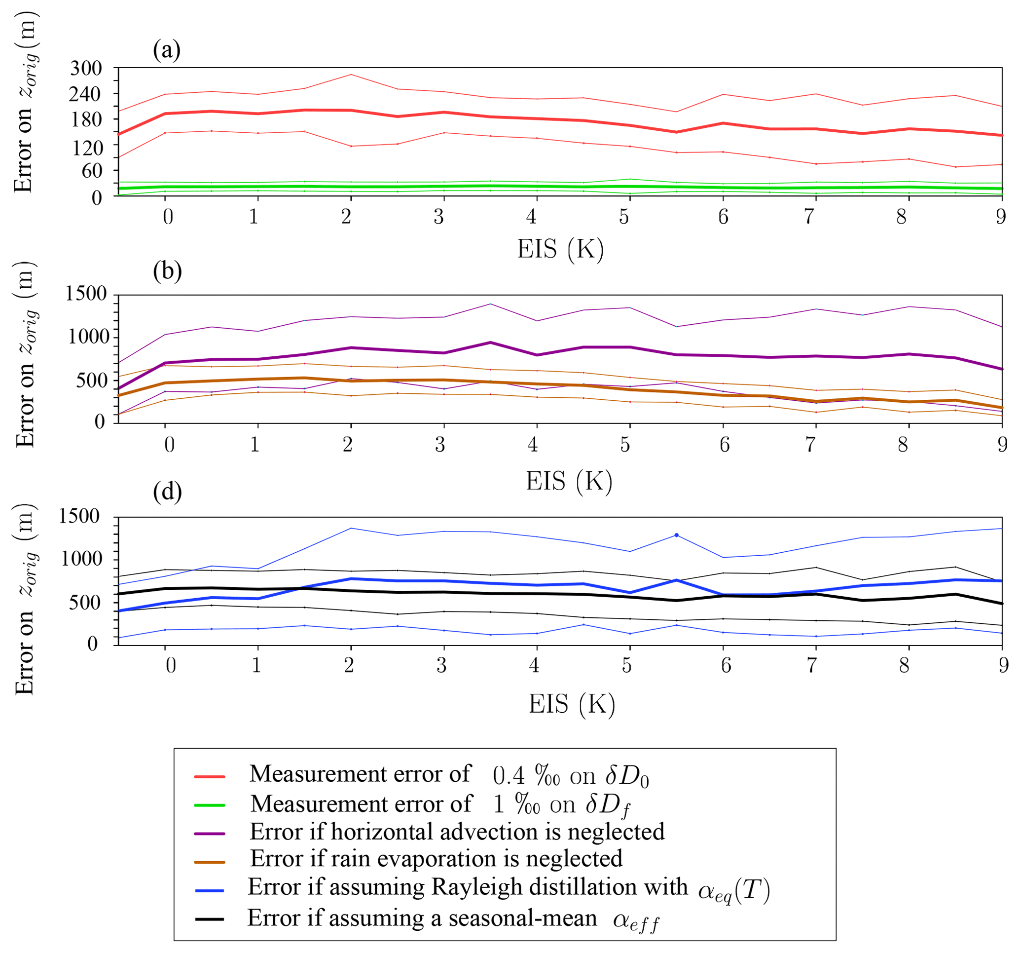
Figure 14Errors when estimating zorig from δD0 observations, as a function of EIS, as predicted by LMDZ. (a) Error we would make if δD0 is measured with a 1 ‰ error (red), and error we would make if δDf is measured with a 1 ‰ error (green). (b) Error we would make if we neglect horizontal advection effects (purple) and rain evaporation effects (brown). (c) Error if one uses αeq as a function of local temperature to estimate αeff (blue), error if one uses the seasonal-mean profile instead of the daily profile to estimate αeff (black). The standard deviations among all daily errors estimated in each bin of EIS are also shown.
We propose an analytical model to predict the water vapor isotopic composition δD0 of the sub-cloud layer (SCL) over tropical oceans. This model relies on the hypothesis that the altitude from which the air originates, zorig, is an important factor. We build on B15, who extended the Merlivat and Jouzel (1979) closure equation to make the explicit link between δD0 and mixing processes. We further extend their equation: we assume a shape for the δD vertical profiles as a function of q, and we account for horizontal advection and rain evaporation effects.
The resulting equation highlights the fact that δD0 is not sensitive to the intensity of mixing processes. Therefore, it is unlikely that water vapor isotopic measurements could help estimate the entrainment velocity that many studies have striven to estimate (Bretherton et al., 1995). In contrast, δD0 is sensitive to the altitude from which the air originates. Based on a simulation with LMDZ and observations during the STRASSE cruise, we show that zorig is an important factor explaining the seasonal spatial and daily variations in δD0, especially in subsidence regions. In turn, could δD0 measurements, combined with vertical profiles of humidity, temperature, and δD, help estimate zorig and thus discriminate between different mixing processes? For such isotope-based estimates of zorig to be useful, we would need a precision of a few hundreds of meters in deep convective regions and smaller than 20 m in stratocumulus regions. To reach this target, we would need daily measurements of δD in the mid-troposphere and very accurate measurements of δD0, which are currently difficult to obtain. We would also need information on the horizontal distribution of δD to account for horizontal advection effects, and full δD profiles to quantify the uncertainty associated with the assumed shape for δD profiles. Finally, rain evaporation is an issue in all regimes, even for stratocumulus clouds. Innovative techniques would need to be developed to quantify this effect from observations.
This study is preliminary in many respects. First, it would be safe to check using water tagging experiments in LMDZ that zorig estimates really represent the altitude from which the air originates and are not biased by our simplifying assumptions. Second, the coarse vertical resolution of LMDZ and the simplicity of mixing parameterizations (e.g., cloud top entrainment is not represented) are a limitation of this study. Ideally, the relationship between δD0, zorig, and the type of mixing processes should be investigated in isotope-enabled large-eddy simulations (LESs) (Blossey et al., 2010; Moore et al., 2014). Artificial tracers and structure detection methods (Park et al., 2016; Brient et al., 2019), combined with conditional sampling methods (Couvreux et al., 2010), could help detect the different kinds of mixing structures, estimate their contributions to vertical transport, and describe their isotopic signature. This would allow us to confirm, or disprove, many of the hypotheses and conclusions in this paper. Finally, if the sensitivity of δD0 to the type of mixing processes is confirmed, paired isotopic simulations of single-column model (SCM) versions of general circulation models (GCMs) and LES, forced by the same forcing, could be very useful to help evaluate and improve the representation of mixing and entrainment processes in GCMs, as is routinely the case for non-isotopic variables (Randall et al., 2003; Hourdin et al., 2013; Zhang et al., 2013).
LMDZ can be downloaded from http://lmdz.lmd.jussieu.fr/ (last access: 26 September 2019). Program codes used for the analysis are available on https://prodn.idris.fr/thredds/catalog/ipsl_public/rlmd698/article_mixing_processes/d_pgmf/catalog.html (last access: 26 September 2019).
Isotopic measurements from STRASSE can be downloaded from http://cds-espri.ipsl.fr/isowvdataatlantic/ (last access: 26 September 2019). All other datasets and processed files are available on https://prodn.idris.fr/thredds/catalog/ipsl_public/rlmd698/article_mixing_processes/catalog.html (last access: 26 September 2019).
For simplicity, we neglect here horizontal advection and rain evaporation effects, but results would be similar otherwise. If we assume that Rorig is uniquely related to qorig through a mixing line between the SCL air and a dry end member (qf, Rf),
and
Reorganizing Eq. (A1), we get with . Since , p≤rorig. Injecting Eq. (A2) into Eq. (6), we get
As a consistency check, in the limit case where the end member is totally dry (p=0), we find the MJ79 equation, i.e., Eq. (10).
It is intriguing to realize that rorig has disappeared from Eq. (A3). This can be understood physically: if the vertical profile follows a mixing line, it does not matter from which altitude the air comes: ultimately, what matters is how much dry air has been mixed directly or indirectly into the SCL (Fig. 4b). Therefore, if Rorig follows a mixing line, we lose the sensitivity to zorig.
Rain evaporation can be accounted for in Eq. (8) if we can quantify η, the ratio of water vapor originating from rain evaporation to that originating from surface evaporation, and αevap, the ratio of isotopic ratio in the rain evaporation flux to R0.
B1 Equations
In LMDZ, two parameterization schemes can produce rain evaporation: the convective scheme and the large-scale condensation scheme. Their respective precipitation evaporation tendencies, and , are given in and are used to calculate Fevap in :
where kLCL is the last layer below the LCL, ΔPk is the depth of layer k in pressure coordinate, and g is gravity.
The isotopic equivalent of this flux, Fevap,iso, is used to calculate .
Only grid boxes and days where Fevap>0.05 mm d−1 are considered to calculate αevap. This represents 94.0 % of all tropical oceanic grid boxes.
B2 Results
Consistent with the larger amount of precipitation available for evaporation, η is at a maximum in regions of deep convection, reaching 30 % around the Maritime Continent (Fig. C1a). It is minimal over the dry descending regions, reaching 5 % off the coasts of Mauritania, Peru, and Namibia. The rain evaporation is more depleted than the SCL in regions of strong deep convection, by as much as 70 ‰ around the Maritime Continent (Fig. C1b). When the fraction of raindrops that evaporate is small, as is the case in such moist regions, isotopic fractionation favors evaporation of the lighter isotopologues. In these regions, rain evaporation has a depleting effect on the SCL, consistent with Worden et al. (2007). In contrast, in other regions, rain evaporation has an enriching effect on the SCL, up to 70 ‰ in dry regions. This is because in dry regions, rain evaporates almost totally, so that the evaporation flux has almost the same composition as the initial rain, which is more enriched than the water vapor.
We can account for horizontal advection in Eq. (8) if we can quantify parameters , the ratio of water vapor coming from horizontal advection to that coming from surface evaporation, and , the ratio of isotopic ratios of horizontal advection to those of the SCL.
C1 Equations
Let us assume that the box representing the SCL has a zonal extent Δy and a meridional extent Δx and is composed of kLCL layers of vertical extent Δzk. The quantity Fadv⋅qadv represents the mass flux of water entering the grid box by horizontal advection per surface area, expressed in . Assuming an upstream advection scheme, it can be expressed as
where uk and vk are the zonal and meridional wind components at layer k, ρk is the volumic mass of air at layer k, and quk and qvk are the humidities of the incoming air from zonal and meridional advection at layer k. When uk>0, quk is the humidity in the grid box to the west. When uk<0, quk is the humidity in the grid box to the east. When vk>0, qvk is the humidity in the grid box to the south. When vk<0, qvk is the humidity in the grid box to the north.
Applying the hydrostatic equation at each layer (, where g is gravity and ΔPk is the vertical extent of the layer k in pressure coordinate), we get
The quantity Fadv represents the incoming air mass flux by horizontal advection, and qadv represents the humidity of the incoming air. We can thus write them as
and
The same budget as in Eq. (C1) can be written for water isotopes:
where Radv represents the isotopic ratio of the incoming water vapor:
Note that the upstream advection scheme assumed here overestimates the effect of advection compared to the Van Leer (1977) advection scheme used in LMDZ. We thus estimate an upper bound for the advection effect here.
In practice, rather than calculating , we calculate , where RSCL is the isotopic ratio on average through the SCL:
This prevents the advected water vapor to be systematically more depleted when the mixed-layer hypothesis is not exactly verified.
C2 Results
Parameter ϕ is at a maximum where winds are maximum, such as near the extra-tropics or in the North Atlantic (Fig. C1a). Horizontal advection has an enriching effect in deep convective regions (probably because water vapor comes from nearby drier regions that have been less depleted by deep convection) and a depleting effect near the coasts (probably because of winds bringing vapor from the nearby land that is depleted by the continental effect) (Fig. C1b).
Note that in this formulation, parameters ϕ and β are resolution-dependent. For example, in a finer resolution, ϕ would be larger and β would be closer to 1, but and thus the contribution of horizontal advection in Eq. (8) would remain the same.
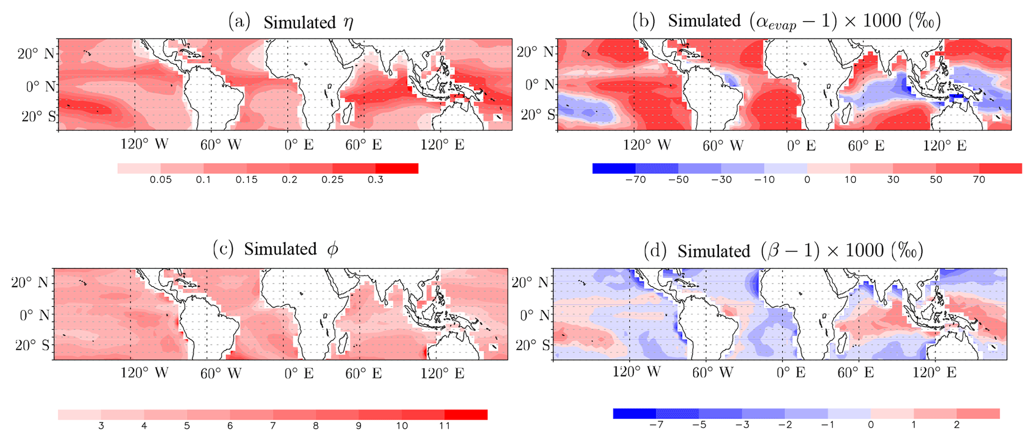
Figure C1(a) Ratio η of water in the SCL coming from rain evaporation to that coming from surface evaporation. (b) Effective fractionation coefficient αevap between the SCL water vapor and the rain evaporation. (c) Ratio ϕ of water in the SCL coming from horizontal advection to that coming from surface evaporation. (d) Effective fractionation coefficient β between the SCL water vapor and the water vapor coming from horizontal advection.
The goal of this appendix is to document the spatiotemporal variability in the shape (Sect. D1) and steepness (Sect. D2) of simulated free-tropospheric δD profiles. Note that a detailed interpretation of these profiles is beyond the scope of this paper. This paper aims at understanding δD0, which is the first step towards understanding full tropospheric profiles. In turn, understanding full tropospheric profiles in future studies will help refine our model for δD0.
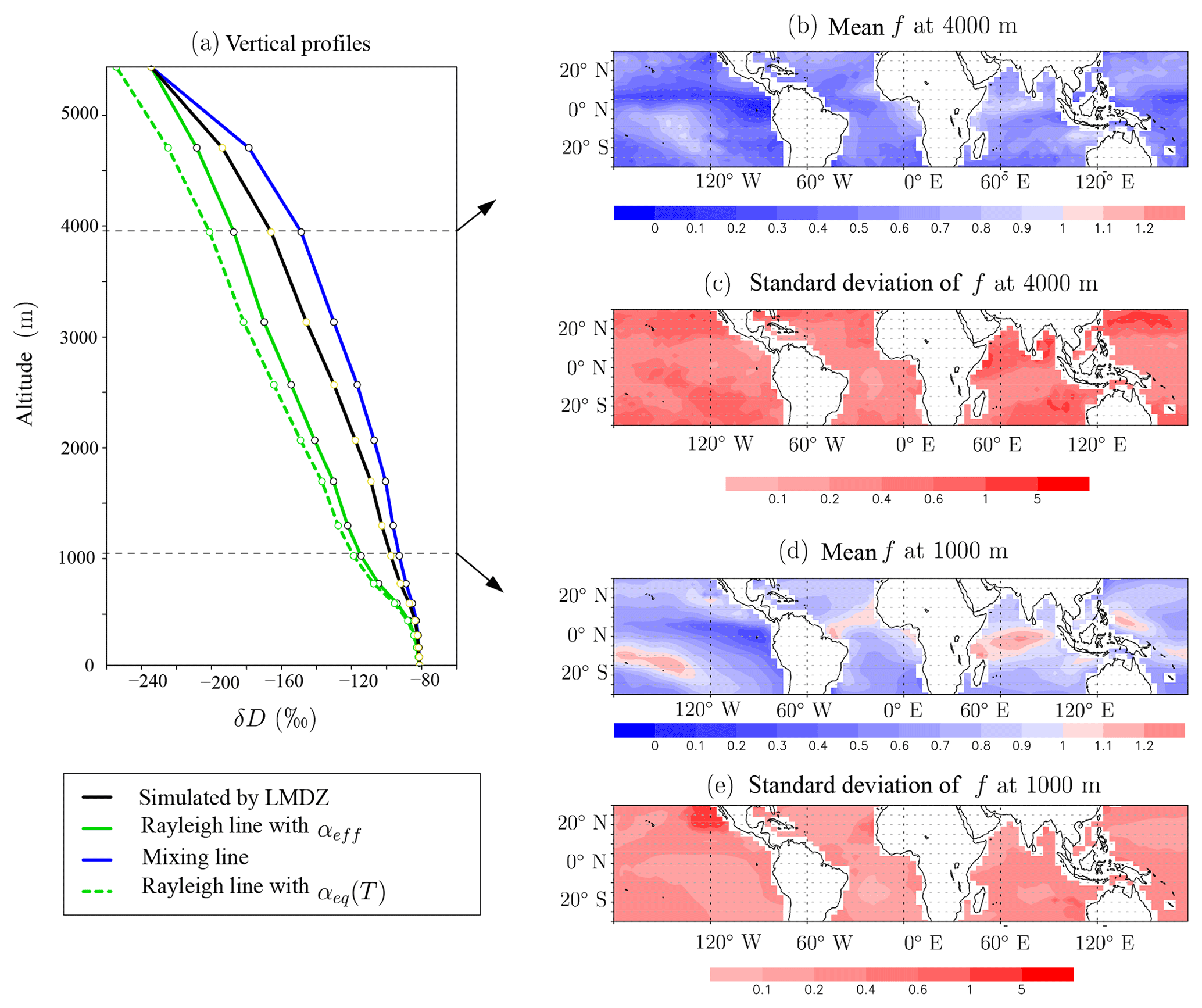
Figure D1(a) Vertical profiles of water vapor δD simulated by LMDZ (black), calculated if assuming a Rayleigh-type curve with αeff estimated from (qf,δDf) at 500 hPa (green), calculated if assuming a Rayleigh-type curve with αeq(T) (dashed green), and calculated if assuming a mixing curve between the first layer and (qf,δDf) at 500 hPa (blue), on average over all tropical oceanic locations and days. (b) Winter-mean map of parameter at 4000 m, i.e., slightly below 500 hPa where qf and δDf are taken. Parameter f describes how close the simulated δD (δDLMDZ) is to the Rayleigh (δDRayleigh) and mixing lines (δDmix): f=0 in case of a Raleigh line, f=1 in case of a mixing line, and f>1 if δD is more enriched than a mixing line. (c) Standard deviation of parameter f among all days in winter of all years, at 4000 m. (d) Same as (b) but at 1000 m, i.e., slightly above the LCL. (e) Same as (c) but at 1000 m. To avoid numerical problems, only days and locations where ‰ are used in the calculations.
D1 Shape of tropospheric profiles
First, we test whether the δD vertical profiles simulated by LMDZ follow a Rayleigh or mixing line as a function of q. For the Rayleigh curve, αeff is estimated as explained in Sect. 3.3. For the mixing line (Appendix A), the end member (qf, Rf) is also taken at 500 hPa.
The tropical-mean vertical δD profiles simulated by LMDZ are bounded by Rayleigh and mixing lines (Fig. D1a). To better document the spatial variability in the shape of δD profiles, we plot parameter , describing how close the simulated δD (δDLMDZ) is to the Rayleigh (δDRayleigh) and mixing (δDmix) lines. We have f=0 in the case of a Raleigh line, f=1 in the case of a mixing line, and f>1 if δD is more enriched than a mixing line. In the lower troposphere, δDLMDZ is close to a mixing line (and sometimes even more enriched) in deep convective regions (Indian Ocean, South Pacific Convergence Zone, Atlantic ITCZ), probably because deep convection efficiently mixes the lower troposphere. Elsewhere, δDLMDZ is intermediate between the two lines (Fig. D1e). In the middle troposphere, δDLMDZ is relatively closer to Rayleigh everywhere (Fig. D1b).
The daily variability of f is large everywhere and at all levels (Fig. D1c, e), with standard deviation of 0.23 and 0.44 on tropical average at 1000 and 4000 m, respectively. A large daily variability in the shape of profiles is also observed in nature (Sodemann et al., 2017).
D2 Steepness of tropospheric profiles
The steepness of the δD gradient from the surface to the middle troposphere is described by the parameter αeff. It is at a maximum in regions of deep convection, for example around the Maritime Continent (Fig. D2a). This is consistent with the maximum depletion simulated in deep convective regions in the mid-troposphere simulated by models (Bony et al., 2008), leading to steeper δD profiles. The pattern of αeff may also reflect horizontal advection effects, where strong isotopic gradients align with winds (e.g., from the eastern to the western Pacific; Dee et al., 2018).
Values of αeff are of the same order of magnitude as real fractionation factors, but the spatial variations do not reflect those predicted if using a fractionation coefficient αeq as a function of temperature T (Fig. D2b).
The daily standard deviation of αeff () for a given season ranges from 5 ‰ in the central Atlantic to 40‰ near the Maritime Continent (Fig. D2c). On average over all seasons and locations, daily αeff−1 at a given location varies within ±25 % of its seasonal-mean mean value.
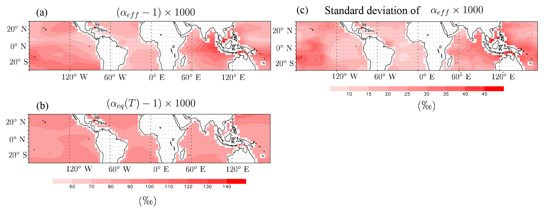
Figure D2(a) αeff−1, where αeff is the effective fractionation coefficient, expressed in per mill. (b) αeq(T)−1 expressed in per mill. All daily values are averaged over all days in winters of all years. (c) Standard deviation of αeff among all days in winter of all years, expressed in per mill.
CR thought about the equations, ran the LMDZ simulations, performed the analysis, and wrote the paper. JG initiated the discussion on the subject and discussed regularly about the results. GR provided the STRASSE radiosoundings. FB provided insight and references about cloud processes. JG, GR, and FB all gave comments on the paper.
The authors declare that they have no conflict of interest.
This work was granted access to the HPC resources of IDRIS under the allocation 2092 made by GENCI. Joseph Galewsky was supported by the LABEX-IPSL visitor program, the Franco-American Fulbright Foundation, and NSF AGS grant 1738075. We thank Marion Benetti and Sandrine Bony for her previous studies on this subject and useful discussions. We thank the two anonymous reviewers for their comments.
This paper was edited by Farahnaz Khosrawi and reviewed by two anonymous referees.
Aemisegger, F., Sturm, P., Graf, P., Sodemann, H., Pfahl, S., Knohl, A., and Wernli, H.: Measuring variations of δ18O and δ2H in atmospheric water vapour using two commercial laser-based spectrometers: an instrument characterisation study, Atmos. Meas. Tech., 5, 1491–1511, https://doi.org/10.5194/amt-5-1491-2012, 2012. a
Aggarwal, P. K., Romatschke, U., Araguas-Araguas, L., Belachew, D., Longstaffe, F. J., Berg, P., Schumacher, C., and Funk, A.: Proportions of convective and stratiform precipitation revealed in water isotope ratios, Nat. Geosci., 9, 624–629, https://doi.org/10.1038/ngeo2739, 2016. a
Bailey, A., Toohey, D., and Noone, D.: Characterizing moisture exchange between the Hawaiian convective boundary layer and free troposphere using stable isotopes in water, J. Geophys. Res.-Atmos., 118, 8208–8221, 2013. a
Benetti, M., Reverdin, G., Pierre, C., Merlivat, L., Risi, C., and Vimeux., F.: Deuterium excess in marine water vapor: Dependency on relative humidity and surface wind speed during evaporation, J. Geophys. Res, 119, 584–593, https://doi.org/10.1002/2013JD020535, 2014. a, b, c, d, e, f, g
Benetti, M., Aloisi, G., Reverdin, G., Risi, C., and Sèze, G.: Importance of boundary layer mixing for the isotopic composition of surface vapor over the subtropical North Atlantic Ocean, J. Geophys. Res.-Atmos., 120, 2190–2209, 2015. a, b, c
Benetti, M., Reverdin, G., Aloisi, G., and Sveinbjörnsdóttir, Á.: Stable isotopes in surface waters of the A tlantic O cean: Indicators of ocean-atmosphere water fluxes and oceanic mixing processes, J. Geophys. Res.-Oceans, 122, 4723–4742, 2017a. a
Benetti, M., Steen-Larsen, H. C., Reverdin, G., Sveinbjörnsdóttir, Á. E., Aloisi, G., Berkelhammer, M. B., Bourlès, B., Bourras, D., De Coetlogon, G., Cosgrove, A., Faber, A.-K., Grelet, J., Hansen, S. B., Johnson, R., Legoff, H., Martin, N., Peters, A. J., Popp, T. J., Reynaud, T., and Winther, M.: Stable isotopes in the atmospheric marine boundary layer water vapour over the Atlantic Ocean, 2012–2015, Sci. Data, 4, 160128, https://doi.org/10.1038/sdata.2016.128, 2017b. a
Betts, A. K. and Ridgway, W.: Climatic equilibrium of the atmospheric convective boundary layer over a tropical ocean, J. Atmos. Sci., 46, 2621–2641, 1989. a, b
Blossey, P. N., Kuang, Z., and Romps, D. M.: Isotopic composition of water in the tropical tropopause layer in cloud-resolving simulations of an idealized tropical circulation, J. Geophys. Res., 115, D24309, https://doi.org/10.1029/2010JD014554, 2010. a
Bolot, M., Legras, B., and Moyer, E. J.: Modelling and interpreting the isotopic composition of water vapour in convective updrafts, Atmos. Chem. Phys., 13, 7903–7935, https://doi.org/10.5194/acp-13-7903-2013, 2013. a
Bony, S., Lau, K., and Sud, Y.: Sea surface temperature and large-scale circulation influences on tropical greenhouse effect and cloud radiative forcing, J. Climate, 10, 2055–2077, 1997. a
Bony, S., Dufresne, J.-L., Le Treut, H., Morcrette, J.-J., and Senior, C.: On dynamic and thermodynamic components of cloud changes, Clim. Dynam., 22, 71–86, https://doi.org/10.1007/s00382-003-0369-6, 2004. a, b
Bony, S., Risi, C., and Vimeux, F.: Influence of convective processes on the isotopic composition (deltaO18 and deltaD) of precipitation and water vapor in the Tropics, Part 1: Radiative-convective equilibrium and TOGA-COARE simulations, J. Geophys. Res., 113, D19305, https://doi.org/10.1029/2008JD009942, 2008. a, b, c, d
Bony, S., Bellon, G., Klocke, D., Sherwood, S., Fermepin, S., and Denvil, S.: Robust direct effect of carbon dioxide on tropical circulation and regional precipitation, Nat. Geosci., 6, 447–451, 2013. a
Bony, S., Stevens, B., Ament, F., Bigorre, S., Chazette, P., Crewell, S., Delanoë, J., Emanuel, K., Farrell, D., Flamant, C., Gross, S., Hirsch, L., Karstensen, J., Mayer, B., Nuijens, L., Ruppert Jr, J. H., Sandu, I., Siebesma, P., Speich, S., Szczap, F., Totems, J., Vogel, R., Wendisch, M., and Wirth, M.: EUREC4A: a field campaign to elucidate the couplings between clouds, convection and circulation, Surv. Geophys., 38, 1529–1568, https://doi.org/10.1007/s10712-017-9428-0, 2017. a
Bretherton, C. S.: Insights into low-latitude cloud feedbacks from high-resolution models, Phil. Trans. R. Soc. A, 373, 20140415, https://doi.org/10.1098/rsta.2014.0415, 2015. a
Bretherton, C. S., Austin, P., and Siems, S. T.: Cloudiness and marine boundary layer dynamics in the ASTEX Lagrangian experiments, Part II: Cloudiness, drizzle, surface fluxes, and entrainment, J. Atmos. Sci., 52, 2724–2735, 1995. a, b, c, d
Brient, F., Couvreux, F., Najda, V., Rio, C., and Honnert, R.: Object-oriented identification of coherent structures in large-eddy simulations: importance of downdrafts in stratocumulus, Geophy. Res. Lett., 46, 2854–2864, https://doi.org/10.1029/2018GL081499, 2019. a, b
Ciais, P., White, W., Jouzel, J., and Petit, J.: The origin of present-day Antarctic precipitation from surface snow deuterium excess data, J. Geophys. Res., 100, 18917–18927, 1995. a, b
Couvreux, F., Hourdin, F., and Rio, C.: Resolved versus parametrized boundary-layer plumes, Part I: A parametrization-oriented conditional sampling in large-eddy simulations, Bound.-Lay. Meteorol., 134, 441–458, 2010. a
Craig, H. and Gordon, L. I.: Deuterium and oxygen-18 variations in the ocean and marine atmosphere, Stable Isotope in Oceanographic Studies and Paleotemperatures, Laboratorio di Geologia Nucleate, Pisa, Italy, 9–130, 1965. a
Dansgaard: Stable isotopes in precipitation, Tellus, 16, 436–468, 1964. a
Davini, P., D'Andrea, F., Park, S.-B., and Gentine, P.: Coherent Structures in Large-Eddy Simulations of a Nonprecipitating Stratocumulus-Topped Boundary Layer, J. Atmos. Sci., 74, 4117–4137, 2017. a, b
De Roode, S. R., Sandu, I., Van Der Dussen, J. J., Ackerman, A. S., Blossey, P., Jarecka, D., Lock, A., Siebesma, A. P., and Stevens, B.: Large-eddy simulations of EUCLIPSE–GASS Lagrangian stratocumulus-to-cumulus transitions: Mean state, turbulence, and decoupling, J. Atmos. Sci., 73, 2485–2508, 2016. a
De Rooy, W. C., Bechtold, P., Fröhlich, K., Hohenegger, C., Jonker, H., Mironov, D., Siebesma, A. P., Teixeira, J., and Yano, J.-I.: Entrainment and detrainment in cumulus convection: An overview, Q. J. Roy. Meteorol. Soc., 139, 1–19, 2013. a
Dee, S. G., Nusbaumer, J., Bailey, A., Russell, J. M., Lee, J.-E., Konecky, B., Buenning, N. H., and Noone, D. C.: Tracking the Strength of the Walker Circulation With Stable Isotopes in Water Vapor, J. Geophys. Res.-Atmos., 123, 7254–7270, 2018. a
Delaygue, G., Masson, V., Jouzel, J., Koster, R. D., and Healy, R. J.: The origin of Antarctic precipitation: A modelling approach, Tellus B, 52, 19–36, 2000. a
Dufresne, J.-L., Foujols, M.-A., Denvil, S., Caubel, A., Marti, O., Aumont, O., alkanski, Y., Bekki, S., Bellenger, H., Benshila, R., Bony, S., Bopp, L., Braconnot, P., Brockmann, P., Cadule, P., Cheruy, F., Codron, F., Cozic, A., Cugnet, D., de Noblet, N., Duvel, J.-P., Ethé, C., Fairhead, L., Fichefet, T., Flavoni, S., Friedlingstein, P., Grandpeix, J.-Y., Guez, L., Guilyardi, E., Hauglustaine, D., Hourdin, F., Idelkadi, A., Ghattas, J., Joussaume, S., Kageyama, M., Krinner, G., Labetoulle, S., Lahellec, A., Lefebvre, M.-P., Lefevre, F., Levy, C., Li, Z. X., Lloyd, J., Lott, F., Madec, G., Mancip, M., Marchand, M., Masson, S., Meurdesoif, Y., Mignot, J., Musat, I., Parouty, S., Polcher, J., Rio, C., Schulz, M., Swingedouw, D., Szopa, S., Talandier, C., Terray, P., and Viovy, N.: Climate change projections using the IPSL-CM5 Earth System Model: from CMIP3 to CMIP5, Clim. Dynam., 40, 1–43, https://doi.org/10.1007/s00382-012-1636-1, 2012. a
Duynkerke, P. G., de Roode, S. R., van Zanten, M. C., Calvo, J., Cuxart, J., Cheinet, S., Chlond, A., Grenier, H., Jonker, P. J., Köhler, M., Lenderink, G., Lewellen, D., Lappen, C., Lock, A. P., Moeng, C., Müller, F., Olmeda, D., Piriou, J.-M., Sánchez, E., and Sednev, I.: Observations and numerical simulations of the diurnal cycle of the EUROCS stratocumulus case, Q. J. Roy. Meteorol. Soc., 130, 3269–3296, 2004. a
Ehhalt, D. H.: Vertical profiles of HTO, HDO, and H2O in the troposphere, NCAR technical note, NCAR-TN-STR-100, 1974. a
Ehhalt, D. H., Rohrer, F., and Fried, A.: Vertical profiles of HDO/H2O in the troposphere, J. Geophy. Res., 110, D13, https://doi.org/10.1029/2004JD005569, 2005. a
Emanuel, K., Neelin, D., and Bretherton, C.: On large-scale circulations in convecting atmospheres, Q. J. Roy. Meteorol. Soc., 120, 1111–1143, 1994. a, b
Ent, R. J. and Savenije, H. H.: Oceanic sources of continental precipitation and the correlation with sea surface temperature, Water Resour. Res., 49, 3993–4004, 2013. a
Faloona, I., Lenschow, D. H., Campos, T., Stevens, B., Van Zanten, M., Blomquist, B., Thornton, D., Bandy, A., and Gerber, H.: Observations of entrainment in eastern Pacific marine stratocumulus using three conserved scalars, J. Atmos. Sci., 62, 3268–3285, 2005. a, b, c
Field, R. D., Jones, D. B. A., and Brown, D. P.: The effects of post-condensation exchange on the isotopic composition of water in the atmosphere, J. Geophy. Res., 115, D24305, https://doi.org/10.1029/2010JD014334, 2010. a
Galewsky, J.: Using Stable Isotopes in Water Vapor to Diagnose Relationships Between Lower-Tropospheric Stability, Mixing, and Low-Cloud Cover Near the Island of Hawaii, Geophys. Res. Lett., 45, 297–305, 2018a. a
Galewsky, J.: Relationships between inversion strength, lower-tropospheric moistening, and low-cloud fraction in the subtropical Southeast Pacific derived from stable isotopologues of water vapor, Geophys. Res. Lett., 45, 7701–7710, 2018b. a
Galewsky, J. and Rabanus, D.: A stochastic model for diagnosing subtropical humidity dynamics with stable isotopologues of water vapor, J. Atmos. Sci., 73, 1741–1753, 2016. a
Galewsky, J. and Samuels-Crow, K.: Water vapor isotopic composition of a stratospheric air intrusion: Measurements from the Chajnantor Plateau, Chile, J. Geophys. Res.-Atmos., 119, 9679–9691, 2014. a
Galewsky, J., Strong, M., and Sharp, Z. D.: Measurements of water vapor D/H ratios from Mauna Kea, Hawaii, and implications for subtropical humidity dynamics, Geophys. Res. Lett., 34, L22808, https://doi.org/10.1029/2007GL031330, 2007. a
Galewsky, J., Steen-Larsen, H. C., Field, R. D., Worden, J., Risi, C., and Schneider, M.: Stable isotopes in atmospheric water vapor and applications to the hydrologic cycle, Rev. Geophys., 54, 809–865, 2016. a
Garratt, J. R.: The atmospheric boundary layer, Earth-Sci. Rev., 37, 89–134, 1994. a
Gates, W. L.: AMIP: The Atmospheric Model Intercomparison Project, B. Am. Meteor. Soc., 73, 1962–1970, 1992. a
Gerber, H., Frick, G., Malinowski, S., Brenguier, J., and Burnet, F.: Holes and entrainment in stratocumulus, J. Atmos. Sci., 62, 443–459, 2005. a, b
Gerber, H., Frick, G., Malinowski, S. P., Jonsson, H., Khelif, D., and Krueger, S. K.: Entrainment rates and microphysics in POST stratocumulus, J. Geophys. Res.-Atmos., 118, 12094–12109, https://doi.org/10.1002/jgrd.50878, 2013. a
Gimeno, L., A., Drumond, R., Nieto, Trigo, R. M., and Stohl, A.: On the origin of continental precipitation, Geophys. Res. Lett., 37, L13804, https://doi.org/10.1029/2010GL043712, 2010. a
Glenn, I. B. and Krueger, S. K.: Downdrafts in the near cloud environment of deep convective updrafts, J. Adv. Model. Earth Syst., 6, 1–8, 2014. a
Good, S. P., Noone, D., Kurita, N., Benetti, M., and Bowen, G. J.: D/H isotope ratios in the global hydrologic cycle, Geophys. Res. Lett., 42, 5042–5050, 2015. a
Graf, P., Wernli, H., Pfahl, S., and Sodemann, H.: A new interpretative framework for below-cloud effects on stable water isotopes in vapour and rain, Atmos. Chem. Phys., 19, 747–765, https://doi.org/10.5194/acp-19-747-2019, 2019. a
Guilpart, E., Vimeux, F., Evan, S., Brioude, J., Metzger, J.-M., Barthe, C., Risi, C., and Cattani, O.: The isotopic composition of near-surface water vapor at the Maïdo observatory (Reunion Island, southwestern Indian Ocean) documents the controls of the humidity of the subtropical troposphere, J. Geophys. Res.-Atmos., 122, 9628–9650, 2017. a
Heus, T. and Jonker, H. J.: Subsiding shells around shallow cumulus clouds, J. Atmos. Sci., 65, 1003–1018, 2008. a, b
Heus, T., Pols, C. F. J., Jonker, H. J., Van den Akker, H. E., and Lenschow, D. H.: Observational validation of the compensating mass flux through the shell around cumulus clouds, Q. J. Roy. Meteorol. Soc., 135, 101–112, 2009. a
Hourdin, F., Musat, I., Bony, S., Braconnot, P., Codron, F., Dufresne, J.-L., Fairhead, L., Filiberti, M.-A., Friedlingstein, P., Grandpeix, J.-Y., Krinner, G., Levan, P., Li, Z.-X., and Lott, F.: The LMDZ4 general circulation model: climate performance and sensitivity to parametrized physics with emphasis on tropical convection, Clim. Dynam., 27, 787–813, https://doi.org/10.1007/s00382-006-0158-0, 2006. a
Hourdin, F., Grandpeix, J.-Y., Rio, C., Bony, S., Jam, A., Cheruy, F., Rochetin, N., Fairhead, L., Idelkadi, A., Musat, I., Dufresne, J.-L., Lahellec, A., Lefebvre, M.-P., and Roehrig, R.: LMDZ5B: the atmospheric component of the IPSL climate model with revisited parameterizations for clouds and convection, Clim. Dynam., 40, 2193–2222, 2013. a
Jonas, P.: Observations of cumulus cloud entrainment, Atmos. Res., 25, 105–127, 1990. a
Jouzel, J. and Koster, R. D.: A reconsideration of the initial conditions used for stable water isotope models, J. Geophys. Res., 101, 22933–22938, https://doi.org/10.1029/96JD02362, 1996. a
Khalsa, S. J. S.: Direct sampling of entrainment events in a marine stratocumulus layer, J. Atmos. Sci., 50, 1734–1750, 1993. a
Kurita, N.: Water isotopic variability in response to mesoscale convective system over the tropical ocean, J. Geophys. Res., 118, 10–376, 2013. a, b
Lacour, J.-L., Clarisse, L., Worden, J., Schneider, M., Barthlott, S., Hase, F., Risi, C., Clerbaux, C., Hurtmans, D., and Coheur, P.-F.: Cross-validation of IASI/MetOp derived tropospheric δD with TES and ground-based FTIR observations, Atmos. Meas. Tech., 8, 1447–1466, https://doi.org/10.5194/amt-8-1447-2015, 2015. a
Lacour, J.-L., Flamant, C., Risi, C., Clerbaux, C., and Coheur, P.-F.: Importance of the Saharan heat low in controlling the North Atlantic free tropospheric humidity budget deduced from IASI δD observations, Atmos. Chem. Phys., 17, 9645–9663, https://doi.org/10.5194/acp-17-9645-2017, 2017a. a
Lacour, J.-L., Risi, C., Worden, J., Clerbaux, C., and Coheur, P.-F.: Isotopic signature of convection's depth in water vapor as seen from IASI and TES D observations, Earth Planet. Sc. Lett., 7, 9645–9663, doi.org/10.5194/acp–17–9645–2017, 2017b. a
Lawrence, J. R., Gedzelman, S. D., Gamache, J., and Black, M.: Stable isotope ratios: Hurricane Olivia, J. Atmos. Chem, 41, 67–82, 2002. a
Lawrence, J. R., Gedzelman, S. D., Dexheimer, D., Cho, H.-K., Carrie, G. D., Gasparini, R., Anderson, C. R., Bowman, K. P., and Biggerstaff, M. I.: Stable isotopic composition of water vapor in the tropics, J. Geophys. Res., 109, D06115, https://doi.org/10.1029/2003JD004046, 2004. a, b, c
Lee, J.-E., Pierrehumbert, R., Swann, A., and Lintner, B. R.: Sensitivity of stable water isotopic values to convective parameterization schemes, Geophys. Res. Lett., 36, L23801, https://doi.org/10.1029/2009GL040880, 2009. a
Lozar, A. and Mellado, J. P.: Evaporative cooling amplification of the entrainment velocity in radiatively driven stratocumulus, Geophys. Res. Lett., 42, 7223–7229, 2015. a
Majoube, M.: Fractionnement en Oxygène 18 et en Deutérium entre l'eau et sa vapeur, Journal de Chimie Physique, 10, 1423–1436, 1971. a
Masunaga, H. and Sumi, Y.: A toy model of tropical convection with a moisture storage closure, J. Adv. Model. Earth Syst., 9, 647–667, 2017. a
McGrath, R., Semmler, T., Sweeney, C., and Wang, S.: Impact of balloon drift errors in radiosonde data on climate statistics, J. Climate, 19, 3430–3442, 2006. a
Mellado, J. P.: Cloud-top entrainment in stratocumulus clouds, Ann. Rev. Fluid Mech., 49, 145–169, 2017. a, b, c
Merlivat, L. and Jouzel, J.: Global climatic interpretation of the Deuterium-Oxygen 18 relationship for precipitation, J. Geophys. Res., 84, 5029–5332, 1979. a, b, c
Moore, M., Kuang, Z., and Blossey, P. N.: A moisture budget perspective of the amount effect, Geophys. Res. Lett., 41, 1329–1335, https://doi.org/10.1002/2013GL058302, 2014. a
Moyer, E. J., Irion, F. W., Yung, Y. L., and Gunson, M. R.: ATMOS stratospheric deuterated water and implications for troposphere-stratosphere transport, Geophys. Res. Lett., 23, 2385–2388, https://doi.org/10.1029/96GL01489, 1996. a
Neggers, R., Stevens, B., and Neelin, J. D.: A simple equilibrium model for shallow-cumulus-topped mixed layers, Theor. Comp. Fluid Dyn., 20, 305–322, 2006. a
Nicholls, S. and Turton, J.: An observational study of the structure of stratiform cloud sheets: Part II, Entrainment, Q. J. Roy. Meteorol. Soc., 112, 461–480, 1986. a
Nuijens, L., Medeiros, B., Sandu, I., and Ahlgrimm, M.: Observed and modeled patterns of covariability between low-level cloudiness and the structure of the trade-wind layer, J. Adv. Model. Earth Syst., 7, 1741–1764, 2015a. a, b
Nuijens, L., Medeiros, B., Sandu, I., and Ahlgrimm, M.: The behavior of trade-wind cloudiness in observations and models: The major cloud components and their variability, J. Adv. Model. Earth Syst., 7, 600–616, 2015b. a, b
Oke, T. R.: Boundary layer climates, Halsted press, New York, 1988. a
Oueslati, B., Bony, S., Risi, C., and Dufresne, J.-L.: Interpreting the inter-model spread in regional precipitation projections in the tropics: role of surface evaporation and cloud radiative effects, Clim. Dynam., 47, 2801–2815, https://doi.org/10.1007/s00382-016-2998-6, 2016. a
Park, S.-B., Gentine, P., Schneider, K., and Farge, M.: Coherent structures in the boundary and cloud layers: Role of updrafts, subsiding shells, and environmental subsidence, J. Atmos. Sci., 73, 1789–1814, 2016. a, b
Randall, D., Krueger, S., Bretherton, C., Curry, J., Duynkerke, P., Moncrieff, M., Ryan, B., Starr, D., Miller, M., Rossow, W., Tselioudis, G. and Wielicki, B.: Confronting models with data: The GEWEX cloud systems study, B. Am. Meteorol. Soc., 84, 455–469, 2003. a
Risi, C., Bony, S., and Vimeux, F.: Influence of convective processes on the isotopic composition (O18 and D) of precipitation and water vapor in the Tropics: Part 2: Physical interpretation of the amount effect, J. Geophys. Res., 113, D19306, https://doi.org/10.1029/2008JD009943, 2008. a
Risi, C., Bony, S., Vimeux, F., Chong, M., and Descroix, L.: Evolution of the water stable isotopic composition of the rain sampled along Sahelian squall lines, Q. J. Roy. Meteor. Soc., 136, 227–242, 2010a. a
Risi, C., Bony, S., Vimeux, F., Frankenberg, C., and Noone, D.: Understanding the Sahelian water budget through the isotopic composition of water vapor and precipitation, J. Geophys. Res, 115, D24110, https://doi.org/10.1029/2010JD014690, 2010b. a, b
Risi, C., Bony, S., Vimeux, F., and Jouzel, J.: Water stable isotopes in the LMDZ4 General Circulation Model: model evaluation for present day and past climates and applications to climatic interpretation of tropical isotopic records, J. Geophys. Res., 115, D12118, https://doi.org/10.1029/2009JD013255, 2010c. a, b
Risi, C., Landais, A., Bony, S., Masson-Delmotte, V., Jouzel, J., and Vimeux, F.: Understanding the 17O-excess glacial-interglacial variations in Vostok precipitation, J. Geophys. Res, 115, D10112, https://doi.org/10.1029/2008JD011535, 2010d. a, b
Risi, C., Noone, D., Worden, J., Frankenberg, C., Stiller, G., Kiefer, M., Funke, B., Walker, K., Bernath, P., Schneider, M., Wunch, D., Sherlock, V., Deutscher, N., Griffith, D., Wernberg, P., Bony, S., Jeonghoon Lee, D. B., Uemura, R., and Sturm, C.: Process-evaluation of tropical and subtropical tropospheric humidity simulated by general circulation models using water vapor isotopic observations, Part 1: model-data intercomparison, J. Geophys. Res., 117, D05303, 2012a. a
Risi, C., Noone, D., Worden, J., Frankenberg, C., Stiller, G., Kiefer, M., Funke, B., Walker, K., Bernath, P., Schneider, M., Wunch, D., Sherlock, V., Deutscher, N., Griffith, D., Wernberg, P., Bony, S., Lee, J., Brown, D., Uemura, R., and Sturm, C.: Process-evaluation of tropical and subtropical tropospheric humidity simulated by general circulation models using water vapor isotopic observations, Part 2: an isotopic diagnostic of the mid and upper tropospheric moist bias, J. Geophys. Res., 117, D05304, 2012b. a, b
Risi, C., Noone, D., Frankenberg, C., and Worden, J.: Role of continental recycling in intraseasonal variations of continental moisture as deduced from model simulations and water vapor isotopic measurements, Water Resour. Res., 49, 4136–4156, https://doi.org/10.1002/wrcr.20312, 2013. a
Rodts, S. M., Duynkerke, P. G., and Jonker, H. J.: Size distributions and dynamical properties of shallow cumulus clouds from aircraft observations and satellite data, J. Atmos. Sci., 60, 1895–1912, 2003. a
Rosenfeld, D. and Mintz, Y.: Evaporation of rain falling from convective clouds as derived from radar measurements, J. Appl. Meteorol., 27, 209–215, 1988. a
Salati, E., Dall'Olio, A., Matsui, E., and Gat, J.: Recycling of water in the Amazon basin: An isotopic study, Water Resour. Res., 15, 1250–1258, 1979. a
Seidel, D. J., Ao, C. O., and Li, K.: Estimating climatological planetary boundary layer hheight from radiosonde observations: comparison of methods and uncertainty analysis, J. Geophys. Res., 115, D16113, https://doi.org/10.1029/2009JD013680, 2010. a
Seidel, D. J., Sun, B., Pettey, M., and Reale, A.: Global radiosonde balloon drift statistics, J. Geophys. Res.-Atmos., 116, https://doi.org/10.1029/2010JD014891, 2011. a
Sherwood, S., Bony, S., and Dufresne, J.-L.: Spread in model climate sensitivity traced to atmospheric convective mixing, Nature, 505, 37–42, https://doi.org/10.1038/nature12829, 2014. a
Sherwood, S. C.: Maintenance of the free tropospheric tropical water vapor distribution, part II: simulation of large-scale advection, J. Climate, 11, 2919–2934, 1996. a
Siebert, P., Beyrich, F., Gryning, S. E., Joffre, S., and Rasmussen, A.: Review and intercomparison of operational methods for the determination of the mixing height, Atmos. Environ., 34, 1001–1027, 2000. a, b
Sodemann, H., Aemisegger, F., Pfahl, S., Bitter, M., Corsmeier, U., Feuerle, T., Graf, P., Hankers, R., Hsiao, G., Schulz, H., Wieser, A., and Wernli, H.: The stable isotopic composition of water vapour above Corsica during the HyMeX SOP1 campaign: insight into vertical mixing processes from lower-tropospheric survey flights, Atmos. Chem. Phys., 17, 6125–6151, https://doi.org/10.5194/acp-17-6125-2017, 2017. a, b, c, d, e, f, g, h, i
Sorbjan, Z.: Structure of the atmospheric boundary layer, Prentice Hall, Englewood Cliffs, N. J., 1989. a
Stevens, B.: Bulk boundary-layer concepts for simplified models of tropical dynamics, Theoret. Comput. Fluid Dynam., 20, 279–304, 2006. a, b
Stewart, M. K.: Stable isotope fractionation due to evaporation and isotopic exchange of falling waterdrops: Applications to atmospheric processes and evaporation of lakes, J. Geophys. Res., 80, 1133–1146, 1975. a
Stull, R. B.: An intruduction to boundary layer meteorology, Kluwer, Dordrect, 1988. a
Taylor, K. E., Stouffer, R. J., and Meehl, G. A.: An overview of CMIP5 and the experiment design, B. Am. Meteorol. Soc., 93, 485–498, 2012. a
Thayer-Calder, K. and Randall, D.: A numerical investigation of boundary layer quasi-equilibrium, Geophys. Res. Lett., 42, 550–556, 2015. a
Tremoy, G., Vimeux, F., Soumana, S., Souley, I., Risi, C., Cattani, O., Favreau, G., and Oi, M.: Clustering mesoscale convective systems with laser-based water vapor δ18O monitoring in Niamey (Niger), J. Geophys. Res., 119, 5079–5103, https://doi.org/10.1002/2013JD020968, 2014. a
Uppala, S., Kallberg, P., Simmons, A., Andrae, U., da Costa Bechtold, V., Fiorino, M., Gibson, J., Haseler, J., Hernandez, A., Kelly, G., Li, X., Onogi, K., Saarinen, S., Sokka, N., Allan, R., Andersson, E., Arpe, K., Balmaseda, M., Beljaars, A., van de Berg, L., Bidlot, J., Bormann, N., Caires, S., Chevallier, F., Dethof, A., Dragosavac, M., Fisher, M., Fuentes, M., Hagemann, S., Holm, E., Hoskins, B., Isaksen, L., Janssen, P., Jenne, R., McNally, A., Mahfouf, J.-F., Morcrette, J.-J., Rayner, N., Saunders, R., Simon, P., Sterl, A., Trenberth, K., Untch, A., Vasiljevic, D., Viterbo, P., and Woollen, J.: The ERA-40 re-analysis, Q. J. Roy. Meteorol. Soc., 131, 2961–3012, 2005. a
Van Leer, B.: Towards the ultimate conservative difference scheme: IV, a new approach to numerical convection, J. Computational Phys., 23, 276–299, 1977. a
Vial, J., Bony, S., Dufresne, J.-L., and Roehrig, R.: Coupling between lower-tropospheric convective mixing and low-level clouds: Physical mechanisms and dependence on convection scheme, J. Adv. Model. Earth Syst., 8, 1892–1911, 2016. a
Wang, Q. and Albrecht, B. A.: Observations of cloud-top entrainment in marine stratocumulus clouds, J. Atmos. Sci., 51, 1530–1547, 1994. a
Webster, C. R. and Heymsfield, A. J.: Water Isotope Ratios D/H, 18O/16O, 17O/16O in and out of Clouds Map Dehydration Pathways, Science, 302, 1742–1746, https://doi.org/10.1126/science.1089496, 2003. a
Williams, K., Ringer, M., and Senior, C.: Evaluating the cloud response to climate change and current climate variability, Clim. Dynam., 20, 705–721, 2003. a
Wood, R.: Stratocumulus clouds, Mon. Weather Rev., 140, 2373–2423, 2012. a
Wood, R. and Bretherton, C. S.: Boundary layer depth, entrainment, and decoupling in the cloud-capped subtropical and tropical marine boundary layer, J. Climate, 17, 3576–3588, 2004. a
Wood, R. and Bretherton, C. S.: On the relationship between stratiform low cloud cover and lower-tropospheric stability, J. Climate, 19, 6425–6432, 2006. a, b, c
Worden, J., Noone, D., and Bowman, K.: Importance of rain evaporation and continental convection in the tropical water cycle, Nature, 445, 528–532, 2007. a, b, c, d, e
Worden, J., Noone, D., Galewsky, J., Bailey, A., Bowman, K., Brown, D., Hurley, J., Kulawik, S., Lee, J., and Strong, M.: Estimate of bias in Aura TES HDO/H2O profiles from comparison of TES and in situ HDO/H2O measurements at the Mauna Loa observatory, Atmos. Chem. Phys., 11, 4491–4503, https://doi.org/10.5194/acp-11-4491-2011, 2011. a
Worden, J., Kulawik, S., Frankenberg, C., Payne, V., Bowman, K., Cady-Peirara, K., Wecht, K., Lee, J.-E., and Noone, D.: Profiles of CH4, HDO, H2O, and N2O with improved lower tropospheric vertical resolution from Aura TES radiances, Atmos. Meas. Tech., 5, 397–411, https://doi.org/10.5194/amt-5-397-2012, 2012. a
Wyant, M. C., Bretherton, C. S., Bacmeister, J. T., Kiehl, J. T., Held, I. M., Zhao, M., Klein, S. A., and Soden, B. J.: A comparison of low-latitude cloud properties and their response to climate change in three AGCMs sorted into regimes using mid-tropospheric vertical velocity, Clim. Dynam., 27, 261–279, 2006. a
Yanai, M., Esbensen, S., and Chu, J.-H.: Determination of bulk properties of tropical cloud clusters from large-scale heat and moisture budgets, J. Atmos. Sci., 30, 611–627, 1973. a
Zhang, M., Bretherton, C. S., Blossey, P. N., Austin, P. H., Bacmeister, J. T., Bony, S., Brient, F., Cheedela, S. K., Cheng, A., Del Genio, A. D., De Roode, S. R., Endo, S., Franklin, C. N., Golaz, J.-C., Hannay, C., Heus, T., Isotta, F. A., Dufresne, J.-L., Kang, I.-S., Kawai, H., Köhler, M., Larson, V. E., Liu, Y., Lock, A. P., Lohmann, U., Khairoutdinov, M. F., Molod, A. M., Neggers, R. A. J., Rasch, P., Sandu, I., Senkbeil, R., Siebesma, A. P., Drian, C. S.-L., Stevens, B., Suarez, M. J., Xu, K.-M., von Salzen, K., Webb, M. J., Wolf, A., Zhao, M.: CGILS: Results from the first phase of an international project to understand the physical mechanisms of low cloud feedbacks in single column models, J. Adv. Model. Earth Syst., 5, 826–842, 2013. a, b
Zipser, E.: Mesoscale and convective scale downdrafts as distinct components of squall-line structure, Mon. Weather Rev., 105, 1568–1589, 1977. a
- Abstract
- Introduction
- Theoretical framework
- Model simulations, observations, and methods
- Results from LMDZ
- Results from observations
- Discussion: what can we learn from water isotopes on mixing processes?
- Conclusions
- Code and data availability
- Appendix A: Closure if the tropospheric profile follows a mixing line
- Appendix B: Diagnostics for rain evaporation in LMDZ
- Appendix C: Diagnostics for horizontal advection in LMDZ
- Appendix D: LMDZ free-tropospheric profiles
- Author contributions
- Competing interests
- Acknowledgements
- Review statement
- References