the Creative Commons Attribution 4.0 License.
the Creative Commons Attribution 4.0 License.
 | 31 Jan 2019
Atmospheric band fitting coefficients derived from a self-consistent rocket-borne experiment
Mykhaylo Grygalashvyly
Martin Eberhart
Jonas Hedin
Boris Strelnikov
Franz-Josef Lübken
Markus Rapp
Stefan Löhle
Stefanos Fasoulas
Mikhail Khaplanov
Jörg Gumbel
Ekaterina Vorobeva
Based on self-consistent rocket-borne measurements of temperature, the densities of atomic oxygen and neutral air, and the volume emission of the atmospheric band (762 nm), we examined the one-step and two-step excitation mechanism of for nighttime conditions. Following McDade et al. (1986), we derived the empirical fitting coefficients, which parameterize the atmospheric band emission . This allows us to derive the atomic oxygen concentration from nighttime observations of atmospheric band emission . The derived empirical parameters can also be utilized for atmospheric band modeling. Additionally, we derived the fit function and corresponding coefficients for the combined (one- and two-step) mechanism. The simultaneous common volume measurements of all the parameters involved in the theoretical calculation of the observed emission, i.e., temperature and density of the background air, atomic oxygen density, and volume emission rate, is the novelty and the advantage of this work.


The mesopause region is essential to understanding the chemical and physical processes in the upper atmosphere because this is the region of coldest temperature (during summer at high latitudes) and highest turbulence in the atmosphere (e.g., Lübken, 1997), the region of formation of such phenomena as noctilucent clouds (NLCs) and polar mesospheric summer echoes (PMSEs) (e.g., Rapp and Lübken, 2004), the region of gravity wave (GW) breaking and the formation of secondary GWs (Becker and Vadas, 2018), and the region of coupling between the mesosphere and thermosphere. This region is characterized by different airglow emissions and, particularly, by the emissions of the atmospheric band, which is produced by the excited state of molecular oxygen . Airglow observation in the atmospheric band is a useful method to study dynamical processes in the mesopause region. There have been a number of reports of GW detection in this band (Noxon, 1978; Viereck and Deehr, 1989; Zhang et al., 1993). Planetary wave climatology has been investigated by the Spectral Airglow Temperature Imager (SATI) instrument (López-González et al., 2009). In addition, the parameters of tides have been reported from SATI (López-González et al., 2005) and high-resolution Doppler imager (HRDI) observations (Marsh et al., 1999). In number of works Sheese et al. (2010, 2011) inferred temperature from atmospheric band observation. Furthermore, the response of mesopause temperature and atomic oxygen during major sudden stratospheric warming was studied utilizing atmospheric band emission by Shepherd et al. (2010). Various works have focused on atmospheric band emission modeling with respect to gravity waves and tides (e.g., Hickey et al., 1993; Leko et al., 2002; Liu and Swenson, 2003). The specific theory of the gravity wave effects on emission was derived in Tarasick and Shepherd (1992). Moreover, atmospheric band observations have been widely utilized to infer atomic oxygen, which is an essential chemical constituent for energetic balance in the extended mesopause region (e.g., Hedin et al., 2009, and references there in), and ozone concentration (Mlynczak et al., 2001). Although there is a large field of application of atmospheric band emissions, there is a lack of knowledge on the processes of the population. Two main mechanisms of nighttime population (note that the daytime mechanisms are quite different; see, e.g., Zarboo et al., 2018) were proposed: the first is the direct population from a three-body recombination of atomic oxygen (e. g. Deans et al., 1976); the second is the so-called two-step mechanism, which assumes an intermediate excited precursor (e. g. Witt et al., 1984; Greer et al., 1981). It has been shown by laboratory experiments that the first mechanism alone has not explained observed emissions (Young and Sharpless, 1963; Clyne at al., 1965; Young and Black, 1966; Bates, 1988). The second mechanism entails a discussion about the precursor excited state and additional ambiguities in their parameters (e.g., Greer et al., 1981; Ogryzlo et al., 1984). Thus, Witt et al. (1984) proposed the hypothesis that the state is, possibly, the precursor; López-González et al. (1992a) suppose that the precursor could be O2(5Πg); and Wildt et al. (1991) found through laboratory measurements that it could be . Hence, the problem of identification is still not solved. The essential step in this direction has been made after the ETON 2 (Energy Transfer in the Oxygen Nightglow) rocket experiment. The ETON 2 mission yielded empirical fitting parameters that allow us to either quantify the (and consequently volume emission) by known O or atomic oxygen by known volume emission values (McDade et al., 1986). Despite the significance of this work, the temperature and density of air (necessary for derivation) were taken from the CIRA-72 and MSIS-83 (Hedin, 1983) models. This leads to some degree of uncertainty (e.g., Murtagh et al., 1990). Thus, more solid knowledge on these fitting coefficients based on consistent measurements of atomic oxygen, the volume emission of the atmospheric band, and temperature and density of the background atmosphere is desirable. In this paper we present common volume measurements of these parameters performed in the course of the WADIS-2 sounding rocket mission. In the next section, we describe the rocket experiment and obtained data relevant for our study. In Sect. 3, to make the paper easier to understand, we repeat some theoretical approximations from McDade et al. (1986). The obtained results of our calculations are discussed in Sect. 4. Concluding remarks and a summary are given in the last section.
The WADIS (Wave propagation and dissipation in the middle atmosphere: Energy budget and distribution of trace constituents) sounding rocket mission aimed to simultaneously study the propagation and dissipation of GWs and measure the concentration of atomic oxygen. It comprised two field campaigns conducted at the Andøya Space Center (ASC) in northern Norway (69∘ N, 16∘ E). The WADIS-2 sounding rocket was launched during the second campaign on 5 March 2015 at 01:44:00 UTC under nighttime conditions. For a more detailed mission description, the reader is referred to Strelnikov et al. (2017) and the accompanying paper by Strelnikov et al. (2018).
The WADIS-2 sounding rocket was equipped with the CONE instrument to measure absolute neutral air density and temperature with high spatial resolution, an instrument for atomic oxygen density measurements (FIPEX; Flux Probe Experiment), and an airglow photometer for atmospheric band (762 nm) volume emission observation.
CONE (COmbined measurement of Neutrals and Electrons), operated by IAP (Leibniz Institute of Atmospheric Physics at Rostock University), is a classical triode-type ionization gauge optimized for a pressure range between 10−5 and 1 mbar. The triode system is surrounded by two electrodes: whilst the outermost grid is biased to +3 to +6 V to measure electron densities at a high spatial resolution, the next inner grid (−15 V) is meant to shield the ionization gauge from ionospheric plasma. CONE is suitable for measuring absolute neutral air number densities at an altitude range between 70 and 120 km. To obtain absolute densities, the gauges are calibrated in the laboratory using a high-quality pressure sensor, like a Baratron. The measured density profile can be further converted to a temperature profile assuming hydrostatic equilibrium. For a detailed description of the CONE instrument, see Giebeler et al. (1993) and Strelnikov et al. (2013). Molecular oxygen and molecular nitrogen are derived from CONE atmospheric number density measurements and partitioning according to the NRLMSISE-00 reference atmosphere (Picone et al., 2002).
The airglow photometer operated by MISU (Stockholm University, Department of Meteorology) measures the emission of the molecular oxygen atmospheric band around 762 nm from the overhead column, from which the volume emission rate is inferred by differentiation. For airglow measurements in general, a filter photometer is positioned under the nose cone viewing along the rocket axis with a defined field of view (FOV). For WADIS-2, however, the FOV of ±3∘ was tilted from the rocket axis by 3∘ to avoid having other parts of the payload within the FOV and at the same time roughly view the same volume as the other instruments. The optical design is a standard radiometer-type system with an objective lens, a field lens, aperture, and stops, which provide an even illumination over a large portion of the detector surface (photomultiplier tube) and a defined FOV. At the entrance of the photometer there is an interference filter with a passband of 6 nm centered at 762 nm. During ascent, after the nose cone ejection, the photometer then counts the incoming photons from the overhead column (or actually the overhead cone). When the rocket passes through the layer the measured photon flux drops and above the emission layer only weak background emissions are present (e.g., the zodiacal and galactic light). After the profile has been corrected for background emissions and attitude (van Rhijn effect) it is converted from counts to radiance using preflight laboratory calibrations. The calibration considers the spectral shape of the 0–0 band of the atmospheric band system and the overlap of the interference filter passband. The profile is then smoothed and numerically differentiated with respect to altitude to yield the volume emission rate of the emitting layer. The data were sampled with 1085 Hz, which results in an altitude resolution of about 0.75 m during the passage of the airglow layer (the velocity was ∼800 m s−1 at 95 km). However, because of the high noise level, the profile needed to be averaged to a vertical resolution of at least 3 km in order to get satisfactory results after the differentiation. A more detailed description and review of this measurement technique is given by Hedin et al. (2009).
The aim of the FIPEX developed by the IRS (Institute of Space Systems, University of Stuttgart) is to measure the atomic oxygen density along the rocket trajectory with high spatial resolution. It employs a solid electrolyte sensor, which has a selective sensitivity to atomic oxygen. A low voltage is applied between anode and cathode pumping oxygen ions through the electrolyte ceramic (yttria-stabilized zirconia). The current measured is proportional to the oxygen density. Sampling is realized with a frequency of 100 Hz and enables a spatial resolution of ∼10 m. Laboratory calibrations were done for molecular and atomic oxygen. For a detailed description of the FIPEX instruments and their calibration techniques, see Eberhart et al. (2015, 2018).
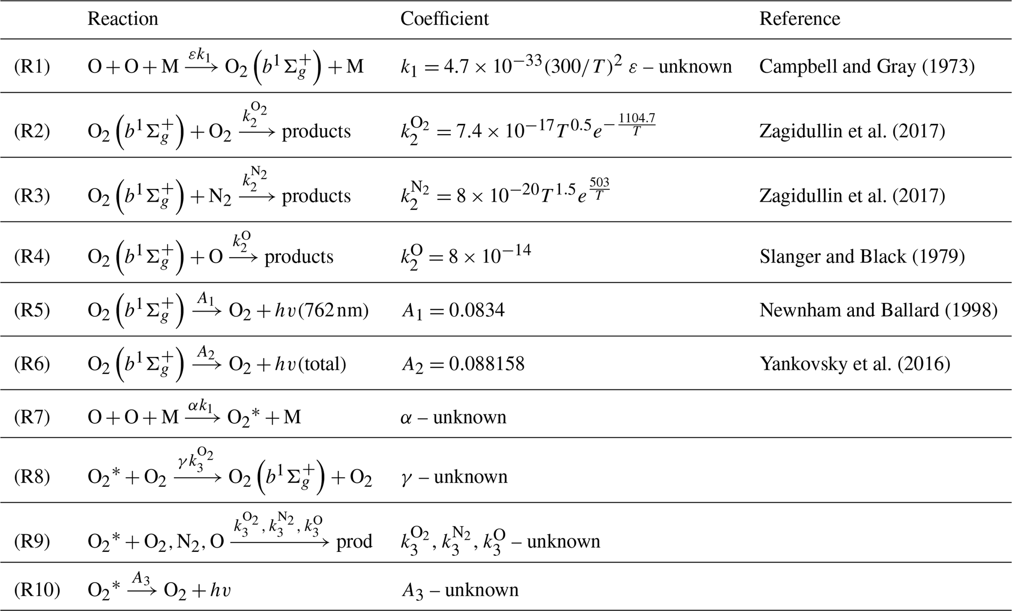
Here, we are repeating the theory of nighttime emissions following McDade et al. (1986) to make our paper more readable, using all nomenclature as in the original paper. All utilized reactions are listed in Table 1, together with corresponding reaction rates, branching ratios, quenching rates, and spontaneous emission coefficients. Some components have been updated according to modern knowledge, thus deviating from the work of McDade et al. (1986).
Table 1List of reactions with corresponding reaction rates (for three-body reactions [cm6 molecule−2 s−1] and for two-body reactions [cm3 molecule−1 s−1]), quenching coefficients, and spontaneous emission coefficients (s−1) used in the paper.
Assuming a direct one-step mechanism as the main one for the population and that is in photochemical equilibrium, we can write its concentration as a ratio of production to the loss term:
where k1 is the reaction rate for the three-body recombination of atomic oxygen, ε is the corresponding quantum yield of formation, A2 represents the spontaneous emission coefficient, and , , are the quenching coefficients for reactions with O2, N2, and O, respectively. Then the volume emission, Vat, is obtained by multiplying the concentration by the spontaneous emission coefficient, A1, of Reaction (R5) (hereafter, nomenclature RX means the reaction X for Table 1).
In the case of known temperature, volume emission, and concentrations of O, O2, N2, and M, the quantum yield of formation can be calculated as follows:
In the case of the two-step mechanism, the unknown excited-state is populated at the first step from Reaction (R7). Then, it can be deactivated by quenching (Reaction R9), spontaneous emission (Reaction R10), or producing by Reaction (R8). Note that Reaction (R8) is one pathway of the overall quenching Reaction (R9).
In the second step, is transformed into , which can be deactivated by quenching (Reactions R2–R4) and by spontaneous emission (Reaction R6). Assuming photochemical equilibrium for and, as before, for , the volume emission in the case of is
where the quantum yield of formation is α, the quantum yield of formation is γ, the spontaneous emission coefficient is A3, and , , are unknown quenching rates of . Note that the assumption about photochemical equilibrium for and is valid because the radiative lifetime is less than 12 s and all potential candidates for have lifetimes less than several seconds (e.g., López-González et al., 1992a, b, c; Yankovsky et al., 2016, and references therein).
Collecting all known values on the right-hand side (RHS), all unknown summands on the left-hand side (LHS), and omitting emissive summand A3 as noneffective loss (McDade et al., 1986), Eq. (3) can be rearranged as follows:
where and are the fitting coefficients that can be calculated by the least-squares fit (LSF) procedure. Such derivation assumes that the coefficients are temperature independent (or temperature dependence is weak). This means that the reaction rates k3 are assumed to be temperature independent (dependence is weak) or have the same temperature dependency for all quenching partners (N2, O2, O). Currently, this statement on the basis of available information about potential precursors is assumed true, but solid evidence is absent. We calculated them based on our measurements and will discuss the results in the following section.
In a more general case the population of occurs via both channels: one-step and two-step. We discuss such processes in Sect. 4.3 and derive an expression for the corresponding fit function in Appendix A.
Figure 1 shows input data for our calculations: temperature from the CONE instrument (Fig. 1a), number density of air (Fig. 1b), atomic oxygen concentration measured by FIPEX (Fig. 1c), and volume emission at 762 nm from the photometric instrument (Fig. 1d). A temperature minimum of ∼158 K was observed at 104.2 km. A local temperature peak was measured at 98.9 km with values of 204.5 K. The secondary temperature minimum was visible at 95.4 km and amounted to ∼173 K. The atomic oxygen concentration (Fig. 1c) had a peak of [cm−3] at 97.2 km and approximately coincided with the secondary temperature peak. The peak of volume emission was detected between 95 and 97 km with values of more than 1700 [phot. cm−3 s−1]; this is slightly beneath the atomic oxygen corresponding maximum and slightly above the secondary temperature minimum. Note that this points to the competition of temperature and the atomic oxygen concentration in processes of atomic oxygen excited-state formation. Independently of the mechanism of atmospheric band emission (Eq. 1 or Eq. 3), the numerator is directly proportional to the square of the atomic oxygen concentration and inversely proportional to the third power of the temperature (via reaction rate k1 and M, considering the ideal gas low). Our rocket experiment shows an essential difference of emissions between ascending and descending flights (see Strelnikov et al., 2018). It also demonstrates significant variability in other measured parameters, including neutral temperature and density as well as atomic oxygen density (Strelnikov et al., 2017, 2018). This suggests that, in the case of the ETON 2 experiments, the temporal extrapolation of atomic oxygen for the time of the emission measurement flight (which was approximately 20 min earlier) may lead to serious biases in estimations because, as one can see from Eqs. (1) and (3), volume emission depends on the atomic oxygen concentration quadratically. Since the best-quality data were obtained during the descent of the WADIS-2 rocket flight, we chose this data set for our analysis (Strelnikov et al., 2018). The region above 104 km is subject to auroral contamination. In the region below 92 km, negative values may occur in the volume emission profile as a result of self-absorption in the denser atmosphere below the emission layer. Hence, we considered the region near the emission peak between 92 and 104 km as most appropriate for our study. The comparisons of our measurements with other observations, as well as with the results of modeling, are presented in several papers (e.g., Eberhart et al., 2018; Strelnikov et al., 2018).
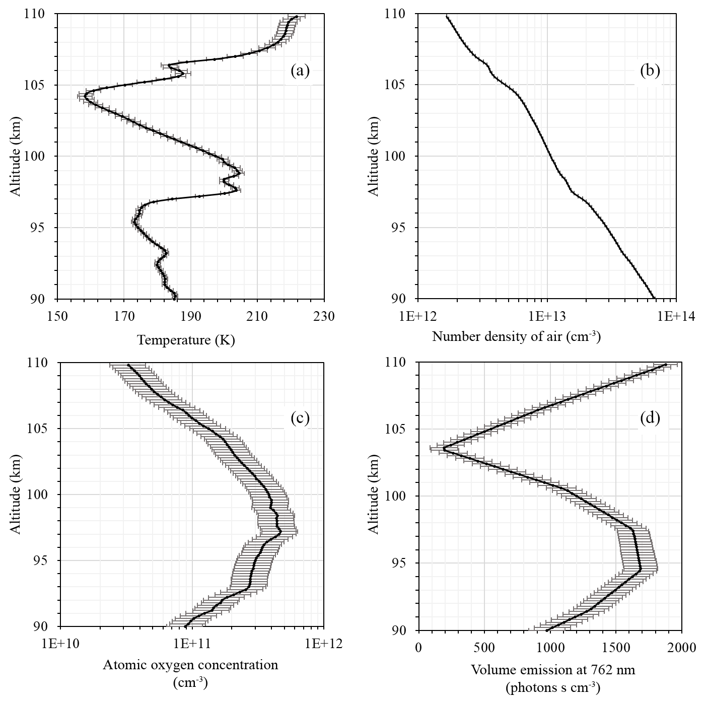
Figure 1Measurements of (a) temperature (CONE), (b) number density of air (CONE), (c) atomic oxygen concentration (FIPEX), and (d) volume emission at 762 nm (photometer).
4.1 One-step mechanism
Figure 2 shows the quantum yield of formation ε calculated according to Eq. (2), which is necessary to form under the assumption that the direct three-body recombination of atomic oxygen is the main mechanism. The uncertainties for this figure (as well as for other figures) were calculated according to a sensitivity analysis (von Clarmann, 2014; Yankovsky and Manuilova, 2018, their Appendix 1; Vorobeva et al., 2018), for which the errors represent error propagation from the experimental data. Calculated values of ε are placed in the range [0.07; 0.13], which is in good agreement with the values derived by McDade et al. (1986). The averaged value amounts to 0.11±0.02. The range of values, taking into account both the variance and the error range, amounts to [0.02; 0.22]. By the physical nature of this value, the quantum yield of formation should not depend on altitude. Figure 2 shows some altitude dependence of central values of ε, but considering the large error range, there is no clear altitude dependence. The variability of the data points is much smaller than the errors of the individual points. Hence, in light of the analysis of our rocket experiment, we may not reject the direct excitation mechanism.
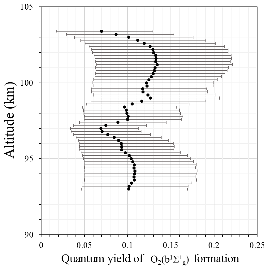
Although the population via the one-step mechanism alone is, generally speaking, possible, it is improbable because laboratory experiments show that direct excitation alone may not explain observed emissions (Young and Sharpless, 1963; Clyne at al., 1965; Young and Black, 1966; Bates, 1988). This conclusion is in agreement with the conclusion from McDade et al. (1986), which stated that the one-step excitation mechanism is not sufficient to explain the population. Hence, in the following, we check the second energy transfer mechanism.
4.2 Two-step mechanism
Figure 3 depicts the altitude profile of the RHS of Eq. (4) and the profile calculated by the LSF. The fitting coefficients, and CO, resulting from this fit amount to and , respectively. The uncertainties were calculated, as is common for LSF (Bevington and Robinson, 2003), based on error propagation from the RHS as provided in Fig. 3. Our coefficient is partially, within the error range, in agreement with coefficients given in McDade et al. (1986), which amount to 4.8±0.3 and 6.6±0.4 for temperature from CIRA-72 and MSIS-83, respectively. The CO coefficient is approximately 1 order lower. There are several possible reasons for the large discrepancy in CO, for example the temperature dependence of the O quenching or that, in the case of ETON 2 experiments, mean temperature profiles from the models CIRA-72 and MSIS-83 were utilized, which does not reproduce any short-time dynamical fluctuations, solar cycle conditions, etc. In the framework of our analysis, we may not identify the reason for the large discrepancy in CO more precisely. Fitting coefficients defined in such a way (Eq. 4) do not have a direct physical meaning. However, they have a physical meaning in several limit cases. If the quenching coefficients of a precursor with molecular nitrogen are much smaller than those with molecular oxygen , then . The assumption that the quenching of the precursor with N2 is much slower than quenching with O2 is just a working hypothesis, which is commonly used for the analysis of possible precursors (e.g., McDade et al., 1986; López-González et al., 1992a, b; and references therein). It is true for such potential precursors as (Kenner and Ogryzlo, 1983b), but generally, there is no evidence for or against that. If it is not true, any definite conclusion on precursors by known is not possible. In our case . In other words, in the case of the two-step formation of with energy transfer agent O2, the total efficiency η=αγ amounts to 10.2 %, which is the lowest amongst known values. Based on rocket experiment data analysis (ETON), Witt et al. (1984) obtained αγ=0.12–0.2. According to McDade et al. (1986) for the case with , the total efficiencies are 0.15 and 0.21 for temperature profiles adopted from MSIS-83 and CIRA-72, respectively. The analyses of López-González et al. (1992a, c), which adopted O2, N2, and temperature profiles from the model (Rodrigo et al., 1991), showed a total efficiency of 0.16. In contrast to our work, all investigations mentioned above utilized temperature and atmospheric density from models that describe a mean state of the atmosphere. This is a possible reason for discrepancy in the results. Total efficiency η may serve as an auxiliary quantity to identify the precursor. According to the physical meaning of efficiency, it may not be larger than 1. Hence, α and γ, as well as the total efficiency, are smaller than 1. Consequently, , and we can examine potential candidates for with this criterion. From an energetic point of view, only four bound states of molecular oxygen can be considered as an intermediate state for the population: , , , and O2(5Πg) (Greer et al., 1981; Wraight, 1982; Witt et al., 1984; McDade et al., 1986; López-González et al., 1992c). For better readability, we will partially repeat a table from López-González et al. (1992b, c) with known α in our work (Table 2). From Table 2, it can be seen that only and O2(5Πg) fit the criterion of . At a lower limit of uncertainty and O2(5Πg) satisfy the criterion and, considering the upper limit (), only O2(5Πg) may serve as a precursor.
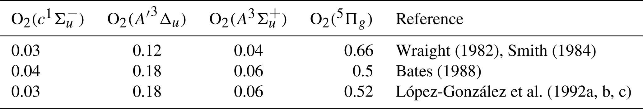

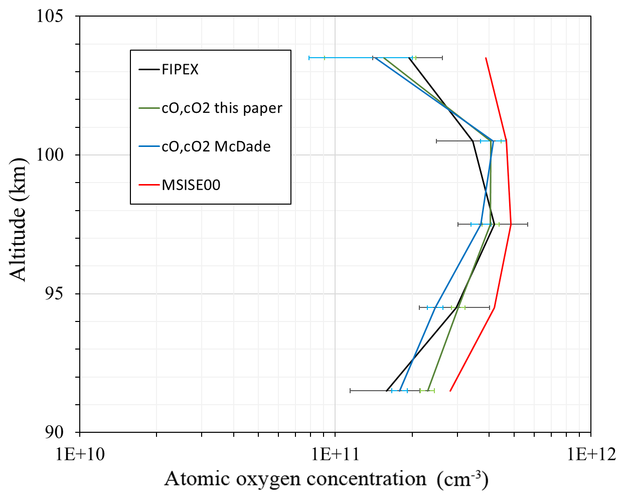
Figure 4Atomic oxygen concentration: FIPEX (black line); model MSIS00 (red line); derived from emission observation with McDade et al. (1986) coefficients (blue line); calculated with newly derived fitting coefficients for the two-step mechanism (green line).
The second expression that helps to clarify the choice of the precursor is the ratio of quenching rates. In the limit of low quenching with molecular nitrogen , the ratio of fitting coefficients equals the ratio of the quenching rates of atomic and molecular oxygen . An analysis from the ETON 2 rocket experiment yields values for the quenching coefficient ratios of potential precursors of 3.1 and 2.9 for temperature from CIRA-72 and MSIS-83, respectively. This is close to the value from Ogryzlo et al. (1984), who found by laboratory measurements; however, as was noted in their work, substitution of these values into the equation for emission yields 16 % of the observed emission (Ogryzlo et al., 1984). These findings point to the possibility of a too-high measured ratio as a result of too-strong quenching of the precursor by atomic oxygen. Our value of quenching ratios amounts to . There is not enough information on measured values for bound states of molecular oxygen. Laboratory measurements for , , and infer the values of the ratio to be 30±30, 100±15, and 200±20, respectively (Kenner and Ogryzlo, 1980, 1983a, b, 1984). On the other hand, Slanger et al. (1984) found that the lower limit of quenching by O2 must be . If the results from Slanger et al. (1984) were applied to the results from Kenner and Ogryzlo (1980, 1984) for , then the ratio of would be 2 orders lower. This short discussion illustrates a strong scattering of this ratio. For our two potential candidates ( and O2(5Πg)), there is information about the ratio for only . Through the comprehensive analysis of known rocket experiments, López-González et al. (1992a, b, c) inferred that the upper limit of the ratio amounts to 1. Hence, our value of agrees with this result. Consistent information from laboratory experiments on the ratio for O2(5Πg) is absent. Thus, we can propose as potential candidates for precursors both and O2(5Πg); however, we are not able to identify which of these two is more preferable.
In order to illustrate the application of the newly derived fitting coefficients we compare in Fig. 4 the atomic oxygen concentration from FIPEX (black line), from the NRL MSISE-00 reference atmosphere model (Picone et al., 2002) (red line) calculated with McDade et al. (1986) coefficients (blue line), and our fitting coefficients for the two-step mechanism (green line). In the region 94–98 km, i.e., at atomic oxygen peak and volume emission peak (see Fig. 1d), fitting coefficients from this paper reproduce observed values better than the McDade coefficients (MSIS-83 case). Our fitting coefficients and the fitting coefficients of McDade give a similar approximation above the atomic oxygen peak (∼98–104 km). The shape of the calculated profiles appears slightly different, with the peak maximum at a higher altitude than the observed. In this, our result resembles the McDade results, probably because in both cases the ratio of two reaction rates is derived, but not the rates themselves. In the lower part our results and those of McDade differ because our value is larger and the term with molecular oxygen dominates. Nevertheless, the atomic oxygen retrieved with our fitting coefficients satisfactorily reproduces measurements, especially at the peak.
4.3 Combined mechanism
In the most general case, the population passes through two channels: directly and via a precursor. In fact, theoretical calculations from Wraight (1982) and laboratory measurements from Bates (1988) predicted a direct population with efficiencies of 0.015 and 0.03, respectively, which is not sufficient to explain the observed emissions (Bates, 1988; Greer et al., 1981; Krasnopolsky, 1986). A similar value, ε=0.02, was shown in the analysis by López-González et al. (1992b, c). We investigated a combined mechanism based on the LSF calculation and fit function (derivation in Appendix A):
where hereafter tildes denote that these are values for the combined mechanism and do not equal the values for one-step or two-step mechanisms (Sect. 4.1 and 4.2); and are the fitting coefficients, which refer to the ratio of quenching rates and total efficiency for the two-step channel, respectively. The fitting coefficients were calculated for two limit cases, (Wraight, 1982) (Bates, 1988), and for the averaged case .
The results for the best fit in each case are listed in Table 3. Analogously to the two-step mechanism (Sect. 4.2), for the case of the combined mechanism ; hence, the precursor should satisfy (see Table 3). For central values of , only and O2(5Πg) satisfy this criterion (see Table 2). At a lower limit of uncertainty (, , and O2(5Πg) satisfy the criterion and, considering the upper limit (), only O2(5Πg) may serve as a precursor. The upper limit of the ratio for , derived by López-González et al. (1992a, b, c), is in agreement with our calculations (). As noted above, the ratio for O2(5Πg) is unknown. Consequently, taking into account both conditions, only and O2(5Πg) may serve as precursors.
Table 3Fitting coefficients for the combined mechanism (Eq. 5) at different efficiencies.
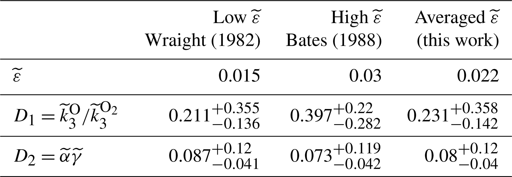
Figure 5 illustrates a sanity check for volume emissions derived (black lines) with the fitting coefficients of McDade et al. (1986) for the MSIS-83 (Fig. 5c) case, the CIRA-72 case (Fig. 5d), and with our newly derived fitting coefficients for the two-step (Fig. 5a) and combined mechanisms (Fig. 5b) in comparison with the measured one (red lines). All of the derived volume emission profiles (black lines) were calculated based on the temperature, concentration of surrounding air, and concentration of atomic oxygen from our rocket launch. The calculations with the combined mechanism (Eq. 5) and two-step energy transfer mechanism (Eq. 4) give almost identical results. The results obtained with the new fitting coefficients are in satisfactory agreement with the measured volume emissions at the peak and above, whereas the McDade coefficients related to temperature from CIRA-72 give better approximations below the volume emission peak (92 km). The coefficients of McDade related to temperature from MSIS-83 are in better agreement with our results and are almost identical above the volume emission peak. More independent common volume in situ measurements are necessary to validate these results.
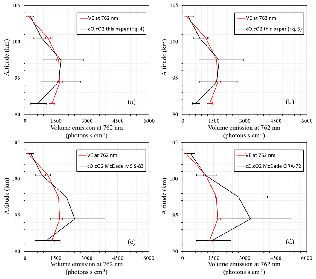
Figure 5Volume emissions: photometer (red line); derived from atomic oxygen (black line) with (a) newly derived fitting coefficients for the two-step mechanism, (b) with fitting coefficients for the combined mechanism, (c) with McDade et al. (1986) coefficients that correspond to MSIS-83 temperature, and (d) with McDade et al. (1986) coefficients that correspond to CIRA-72 temperature.
Based on the rocket-borne common volume simultaneous observations of atomic oxygen, atmospheric band emission (762 nm), and density and temperature of the background atmosphere, the mechanisms of formation were analyzed. Our calculations show that one-step direct excitation alone is less probable for the reasons discussed above (Sect. 4.1).
For the case of the two-step mechanism, we found new coefficients for the fit function in accordance with McDade et al. (1986) based on self-consistent temperature, atomic oxygen, and volume emission observation. These coefficients amounted to and . The coefficient is partially, within the error range, in agreement with coefficients given in McDade et al. (1986), and the CO coefficient is approximately 1 order lower. The general implication of these results is the parameterization of volume emission in terms of known atomic oxygen. This can be utilized either for atmospheric band volume emission modeling or for the estimation of atomic oxygen by known volume emission. We identified two candidates for the intermediate state of . Our results show that or O2(5Πg) may serve as a precursor.
Taking into account both channels of formation, we proposed a combined mechanism. In this case, atomic oxygen via volume emission or volume emission based on known atomic oxygen can be calculated by Eq. (5). The recommended fitting coefficients amounted to and , with the efficiency of the direct channel as . These coefficients have a mean total efficiency and a ratio of quenching coefficients ( for the two-step channel. The analysis of their values indicates that and O2(5Πg) may serve as possible precursors for the two-step channel in the combined mechanism. In the context of our rocket experiment, we do not have the possibility to figure out which mechanism is true. Nevertheless, we consider the combined mechanism as more relevant to nature because it has a higher generality. This conclusion does not contradict the current point of view that the two-step mechanism is dominant because is assumed to be 1.5 %–3 %. Moreover, it is possible that in reality the mechanism is much more complex and it has a multichannel or more than two-step nature. Undoubtedly, more common volume simultaneous observations of the atmospheric band and atomic oxygen concentrations would be desirable to confirm and improve these results.
The rocket-borne measurements and calculated data shown in this paper are available via the IAP ftp server at ftp://ftp.iap-kborn.de/data-in-publications/GrygalashvylyACP2018 (last access: 25 January 2019).
We consider photochemical equilibrium for the nighttime concentration. If is produced via both channels, the equilibrium concentration is given by the following expression:
where the tilde denotes the combined mechanism, A1, , , , are the ratios for the corresponding processes (see Table 1), and is the unknown precursor.
Considering this precursor in photochemical equilibrium, we can obtain the following expression for its concentration:
where efficiency is , is the unknown spontaneous emission coefficient of , and , , are the unknown quenching rates for .
Substituting (A2) into (A1) and into the expression for volume emission we obtain
We assume that, in analogy with a two-step mechanism, a spontaneous emission of is much smaller than the quenching, and we utilized a traditional assumption about low quenching with molecular nitrogen , which is commonly used to analyze a potential precursor. In this case, Eq. (A3) can be rearranged as follows:
We defined unknown fitting coefficients and . Expression (A4) was utilized to calculate them with LSF.
The authors contributed equally to this work.
The authors declare that they have no conflict of interest.
This article is part of the special issue “Layered phenomena in the mesopause region (ACP/AMT inter-journal SI)”. It is a result of the LPMR workshop 2017 (LPMR-2017), Kühlungsborn, Germany, 18–22 September 2017.
The authors are thankful to Valentin Andreevich Yankovsky, William Ward, and Gerd Reinhold Sonnemann for helpful suggestions and useful discussions. This work was supported by the German Space Agency (DLR) under grant 50 OE 1001 (project WADIS). The authors thank DLR-MORABA for their excellent contribution to the project by developing the complicated WADIS payload and campaign support together with the Andøya Space Center, as well as Hans-Jürgen Heckl and Torsten Köpnick for building the rocket instrumentation. The authors are thankful to coeditor Bernd Funke for help in evaluating this paper and to three anonymous referees for their useful comments and improvements to the paper.
The publication of this article was funded by the
Open Access
Fund of the Leibniz Association.
Edited by: Bernd Funke
Reviewed by: Miriam Sinnhuber and two anonymous referees
Bates, D. R.: Excitation and quenching of the oxygen bands in the nightglow, Planet. Space Sci., 36, 875–881, 1988.
Becker, E. and Vadas, S. L.: Secondary gravity waves in the winter mesosphere: Results from a high-resolution global circulation model, J. Geophys. Res., 123, 2605–2627, https://doi.org/10.1002/2017JD027460, 2018.
Bevington, P. R. and Robinson, D. K.: Data reduction and error analysis for the physical sciences, 3rd edn., McGraw-Hill Companies Inc., New York, USA, 2003.
Campbell, I. M. and Gray, C. N.: Rate constants for O(3P) recombination and association with N(4S), Chem. Phys. Lett., 18, 607–609, https://doi.org/10.1016/0009-2614(73)80479-8, 1973, 1973.
Clyne, M. A. A., Thrush, B. A., and Wayne, R. P.: The formation and reactions of metastable oxygen molecules, J. Photochem. Photobiol., 4, 957–961, 1965.
Deans, A. J., Shepherd, G. G., and Evans, W. F. J.: A rocket measurement of the atmospheric band nightglow altitude distribution, Geophys. Res. Lett., 3, 441–444, 1976.
Eberhart, M., Löhle, S., Steinbeck, A., Binder, T., and Fasoulas, S.: Measurement of atomic oxygen in the middle atmosphere using solid electrolyte sensors and catalytic probes, Atmos. Meas. Tech., 8, 3701–3714, https://doi.org/10.5194/amt-8-3701-2015, 2015.
Eberhart, M., Löhle, S., Strelnikov, B., Hedin, J., Khaplanov, M., Fasoulas, S., Gumbel, J., Lübken, F.-J., and Rapp, M.: Atomic oxygen number densities in the MLT region measured by solid electrolyte sensors on WADIS-2, Atmos. Meas. Tech. Discuss., https://doi.org/10.5194/amt-2018-341, in review, 2018.
Giebeler, J., Lübken, F.-J., and Nägele, M.: CONE – a new sensor for in-situ observations of neutral and plasma density fluctuations, ESA SP, Montreux, Switzerland, ESA-SP-355, 311–318, 1993.
Greer, R. G. H., Llewellyn, E. J., Solheim, B. H., and Witt, G.: The excitation of O2() in the nightglow, Planet. Space Sci., 29, 383–389, 1981.
Hedin, A. E.: A revised thermospheric model based on mass spectrometer and incoherent scatter data: MSIS-83, J. Geophys. Res., 88, 10170–10188, 1983.
Hedin, J., Gumbel, J., Stegman, J., and Witt, G.: Use of O2 airglow for calibrating direct atomic oxygen measurements from sounding rockets, Atmos. Meas. Tech., 2, 801–812, https://doi.org/10.5194/amt-2-801-2009, 2009.
Hickey, M. P., Schubert, G., and Walterscheid, R. L.: Gravity wave-driven fluctuations in the O2 atmospheric (0–1) nightglow from an extended, dissipative emission region, J. Geophys. Res., 98, 717–730, 1993.
Kenner, R. D. and Ogryzlo, E. A.: Deactivation of O2() by O2, O and Ar, Int. J. Chem. Kinet., 12, 501–508, 1980.
Kenner, R. D. and Ogryzlo, E. A.: Quenching of O2( by O(3P), O2(a1Δg) and other gases, Can. J. Chem., 61, 921–926, 1983a.
Kenner, R. D. and Ogryzlo, E. A.: Rate constant for the deactivation of O2() by N2, Chem. Phys. Lett., 103, 209–212, 1983b.
Kenner, R. D. and Ogryzlo, E. A.: Quenching of O2() Herzberg I band by O2(a) and O, Can. J. Phys., 62, 1599–1602, 1984.
Krasnopolsky, V. A.: Oxygen emissions in the night airglow of the Earth, Venus and Mars, Planet. Space Sci., 34, 511–518, 1986.
Leko, J. J., M. P. Hickey, and Richards, P. G.: Comparison of simulated gravity wave-driven mesospheric airglow fluctuations observed from the ground and space, J. Atmos. Sol.-Terr. Phy., 64, 397–403, 2002.
Liu, A. Z. and Swenson, G. R.: A modeling study of O2 and OH airglow perturbations induced by atmospheric gravity waves, J. Geophys, Res., 108, 4151, https://doi.org/10.1029/2002JD002474, 2003.
López-González, M. J., López-Moreno, J. J., and Rodrigo, R.: Altitude profiles of the atmospheric system of O2 and of the green line emission, Planet. Space Sci., 40, 783–795, 1992a.
López-González, M. J., López-Moreno, J. J., and Rodrigo, R.: Altitude and vibrational distribution of the O2 ultraviolet nightglow emissions, Planet. Space Sci., 40, 913–928, 1992b.
López-González, M. J., López-Moreno, J. J., and Rodrigo, R.: Atomic oxygen concentrations from airglow measurements of atomic and molecular oxygen emissions in the nightglow, Planet. Space Sci., 40, 929–940, 1992c.
López-González, M. J., Rodríguez, E., Shepherd, G. G., Sargoytchev, S., Shepherd, M. G., Aushev, V. M., Brown, S., García-Comas, M., and Wiens, R. H.: Tidal variations of O2 Atmospheric and OH(6–2) airglow and temperature at mid-latitudes from SATI observations, Ann. Geophys., 23, 3579–3590, https://doi.org/10.5194/angeo-23-3579-2005, 2005.
López-González, M. J., Rodríguez, E., García-Comas, M., Costa, V., Shepherd, M. G., Shepherd, G. G., Aushev, V. M., and Sargoytchev, S.: Climatology of planetary wave type oscillations with periods of 2–20 days derived from O2 atmospheric and OH(6–2) airglow observations at mid-latitude with SATI, Ann. Geophys., 27, 3645–3662, https://doi.org/10.5194/angeo-27-3645-2009, 2009.
Lübken, F.-J.: Seasonal variation of turbulent energy dissipation rates at high latitudes as determined by in situ measurements of neutral density fluctuations, J. Geophys. Res., 102, 13441–13456, 1997.
McDade, I. C., Murtagh, D. P., Greer, R. G. H., Dickinson, P. H. G., Witt, G., Stegman, J., Llewellyn, E. J., Thomas, L., and Jenkins, D. B.: ETON 2: Quenching parameters for the proposed precursors of O2 and O(1S) in the terrestrial nightglow, Planet. Space Sci., 34, 789–800, 1986.
Mlynczak, M. G., Morgan, F., Yee, J.-H., Espy, P., Murtagh, D., Marshall, B., Schmidlin, F.: Simultaneous measurements of the O2(1Δ) and O2(1Σ) airglows and ozone in the daytime mesosphere, Geophys. Res. Lett., 28, 999–1002, 2001.
Murtagh, D. P., Witt, G., Stegman, J., McDade, I. C., Llewellyn, E. J., Harris, F., and Greer, R. G. H.: An assessment of proposed O(1S) and O2 nightglow excitation parameters, Planet. Space Sci., 38, 45–53, 1990.
Newnham, D. A. and Balard, J.: Visible absorption cross sections and integrated absorption intensities of molecular oxygen (O2 and O4), J. Geophys, Res., 103, 28801–28815, 1998.
Noxon, J. F.: Effect of Internal Gravity Waves Upon Night Airglow Temperatures, Geophys. Res. Lett., 5, 25–27, 1978.
Ogryzlo, E. A., Shen, Y. Q., and Wassel, P. T.: The yield of O2 in oxygen atom recombination, J. Photochem., 25, 389–398, 1984.
Picone, J. M., Hedin, A. E., Drob, D. P., and Aikin, A. C.: NRLMSISE-00 empirical model of the atmosphere: Statistical comparisons and scientific issues, J. Geophys. Res., 107, 1468, https://doi.org/10.1029/2002JA009430, 2002.
Rapp, M. and Lübken, F.-J.: Polar mesosphere summer echoes (PMSE): Review of observations and current understanding, Atmos. Chem. Phys., 4, 2601–2633, https://doi.org/10.5194/acp-4-2601-2004, 2004.
Rodrigo, R., López-González, M. J., and López-Moreno, J. J.: Variability of the neutral mesospheric and lower thermospheric composition in the diurnal cycle, Planet. Space Sci., 39, 803–820, 1991.
Sheese, P. E., Llewellyn, E. J., Gattinger, R. L., Bourassa, A. E., Degenstein, D. A., Lloyd, N. D., and McDade I. C.: Temperatures in the upper mesosphere and lower thermosphere from OSIRIS observations of O2 A-band emission spectra, Can. J. Phys., 88, 919–925, https://doi.org/10.1139/P10-093, 2010.
Sheese, P. E., Llewellyn, E. J., Gattinger, R. L., Bourassa, A. E., Degenstein, D. A., Lloyd, N. D., and McDade I. C.: Mesopause temperatures during the polar mesospheric cloud season, Geophys. Res. Lett., 38, L11803, https://doi.org/10.1029/2011GL047437, 2011.
Shepherd, M. G., Cho, Y.-M., Shepherd, G. G., Ward, W., and Drummond, J. R.: Mesospheric temperature and atomic oxygen response during the January 2009 major stratospheric warming, J. Geophys. Res., 115, A07318, https://doi.org/10.1029/2009JA015172, 2010.
Slanger, T. G. and Black, G.: Interactions of O2() with O(3P) and O3, J. Chem. Phys., 70, 3434–3438, 1979.
Slanger, T. G., Bischel, W. K., and Dyer, M. J.: Photoexcitation of O2 at 249.3 nm, Chem. Phys. Lett., 108, 472–474, 1984.
Smith, I. W. M.: The role of electronically excited states in recombination reactions, Int. J. Chem. Phys., 16, 423–443, 1984.
Strelnikov, B., Rapp, M., and Lübken, F.-J.: In-situ density measurements in the mesosphere/lower thermosphere region with the TOTAL and CONE instruments, in: An Introduction to Space Instrumentation, edited by: Oyama, K., Terra Publishers, https://doi.org/10.5047/isi.2012.001, 2013.
Strelnikov, B., Szewczyk, A., Strelnikova, I., Latteck, R., Baumgarten, G., Lübken, F.-J., Rapp, M., Fasoulas, S., Löhle, S., Eberhart, M., Hoppe, U.-P., Dunker, T., Friedrich, M., Hedin, J., Khaplanov, M., Gumbel, J., and Barjatya, A.: Spatial and temporal variability in MLT turbulence inferred from in situ and ground-based observations during the WADIS-1 sounding rocket campaign, Ann. Geophys., 35, 547–565, https://doi.org/10.5194/angeo-35-547-2017, 2017.
Strelnikov, B., Staszak, T., Asmus, H., Strelnikova, I., Latteck, R., Grygalashvyly, M., Lübken, F.-J., Baumgarten, G., Höffner, J., Wörl, R., Hedin, J., Khaplanov, M., Gumbel, J., Eberhart, M., Löhle, S., Fasoulas, S., Rapp, M., Friedrich, M., Williams, B. P., Barjatya, A., Taylor, M. J., and Pautet, P.-D.: Simultaneous in situ measurements of small-scale structures in neutral, plasma, and atomic oxygen densities during WADIS sounding rocket project, Atmos. Chem. Phys., submitted, 2018.
Tarasick, D. W. and Shepherd, G. G.: Effects of gravity waves on complex airglow chemistries. 2. OH emission, J. Geophys. Res., 97, 3195–3208, 1992.
Viereck, R. A. and Deehr, C. S.: On the interaction between gravity waves and the OH Meinel (6–2) and O2 Atmospheric (0–1) bands in the polar night airglow, J. Geophys. Res., 94, 5397–5404, 1989.
von Clarmann, T.: Smoothing error pitfalls, Atmos. Meas. Tech., 7, 3023–3034, https://doi.org/10.5194/amt-7-3023-2014, 2014.
Vorobeva, E., Yankovsky, V., and Schayer, V.: Estimation of uncertainties of the results of [O(3P)], [O3] and [CO2] retrievals in the mesosphere according to the YM2011 model by two approaches: sensitivity study and Monte Carlo method, EGU General Assembly, Vienna, Austria, 8–13 April 2018, EGU2018-AS1.31/ST3.7-17950, available at: https://presentations.copernicus.org/EGU2018-17950_presentation.pdf (last access: 26 January 2019), 2018.
Wildt, J., Bednarek, G., Fink, E. H., Wayne, R. P.: Laser excitation of the A, A and c1Σu− states of molecular oxygen, Chem. Phys., 156, 497–508, https://doi.org/10.1016/0301-0104(91)89017-5, 1991.
Witt, G., Stegman, J., Murtagh, D. P., McDade, I. C., Greer, R. G. H., Dickinson, P. H. G., and Jenkins, D. B.: Collisional energy transfer and the excitation of O2() in the atmosphere, J. Photochem., 25, 365–378, 1984.
Wraight, P. C.: Association of atomic oxygen and airglow excitation mechanisms, Planet. Space Sci., 30, 251–259, 1982.
Yankovsky, V. A. and Manuilova, R. O.: Possibility of simultaneous [O3] and [CO2] altitude distribution retrievals from the daytime emissions of electronically-vibrationally excited molecular oxygen in the mesosphere, J. Atmos. Sol.-Terr. Phy., 179, 22–33, https://doi.org/10.1016/j.jastp.2018.06.008, 2018.
Yankovsky, V. A., Martysenko, K. V., Manuilova, R. O., and Feofilov, A. G.: Oxygen dayglow emissions as proxies for atomic oxygen and ozone in the mesosphere and lower thermosphere, J. Mol. Spectrosc., 327, 209–231, https://doi.org/10.1016/j.jms.2016.03.006, 2016.
Young, R. A. and Black, G.: Excited state formation and destruction in mixtures of atomic oxygen and nitrogen, J. Chem. Phys., 44, 3741, https://doi.org/10.1063/1.1726529, 1966.
Young, R. A. and Sharpless, R. L.: Chemiluminescence and reactions involving atomic oxygen and nitrogen, J. Chem. Phys., 39, 1071, https://doi.org/10.1063/1.1734361, 1963.
Zagidullin, M. V., Khvatov, N. A., Medvedkov, I. A., Tolstov, G. I., Mebel, A. M., Heaven, M. C., and Azyazov, V. N.: O2() Quenching by O2, CO2, H2O, and N2 at Temperatures of 300–800 K, J. Phys. Chem., 121, 7343–7348, https://doi.org/10.1021/acs.jpca.7b07885, 2017.
Zarboo, A., Bender, S., Burrows, J. P., Orphal, J., and Sinnhuber, M.: Retrieval of O2(1Σ) and O2(1Δ) volume emission rates in the mesosphere and lower thermosphere using SCIAMACHY MLT limb scans, Atmos. Meas. Tech., 11, 473–487, https://doi.org/10.5194/amt-11-473-2018, 2018.
Zhang, S. P., Wiens, R. H., and Shepherd, G. G.: Gravity waves from O2 nightglow during the AIDA '89 campaign II: numerical modeling of the emission rate/temperature ratio, η, J. Atmos. Terr. Phys., 55, 377–395, 1993.