the Creative Commons Attribution 4.0 License.
the Creative Commons Attribution 4.0 License.
 | 04 Sep 2019
The importance of the representation of air pollution emissions for the modeled distribution and radiative effects of black carbon in the Arctic
Jacob Schacht
Bernd Heinold
Johannes Quaas
John Backman
Ribu Cherian
Andre Ehrlich
Andreas Herber
Wan Ting Katty Huang
Yutaka Kondo
Andreas Massling
P. R. Sinha
Bernadett Weinzierl
Marco Zanatta
Ina Tegen
Aerosol particles can contribute to the Arctic amplification (AA) by direct and indirect radiative effects. Specifically, black carbon (BC) in the atmosphere, and when deposited on snow and sea ice, has a positive warming effect on the top-of-atmosphere (TOA) radiation balance during the polar day. Current climate models, however, are still struggling to reproduce Arctic aerosol conditions. We present an evaluation study with the global aerosol-climate model ECHAM6.3-HAM2.3 to examine emission-related uncertainties in the BC distribution and the direct radiative effect of BC. The model results are comprehensively compared against the latest ground and airborne aerosol observations for the period 2005–2017, with a focus on BC. Four different setups of air pollution emissions are tested. The simulations in general match well with the observed amount and temporal variability in near-surface BC in the Arctic. Using actual daily instead of fixed biomass burning emissions is crucial for reproducing individual pollution events but has only a small influence on the seasonal cycle of BC. Compared with commonly used fixed anthropogenic emissions for the year 2000, an up-to-date inventory with transient air pollution emissions results in up to a 30 % higher annual BC burden locally. This causes a higher annual mean all-sky net direct radiative effect of BC of over 0.1 W m−2 at the top of the atmosphere over the Arctic region (60–90∘ N), being locally more than 0.2 W m−2 over the eastern Arctic Ocean. We estimate BC in the Arctic as leading to an annual net gain of 0.5 W m−2 averaged over the Arctic region but to a local gain of up to 0.8 W m−2 by the direct radiative effect of atmospheric BC plus the effect by the BC-in-snow albedo reduction. Long-range transport is identified as one of the main sources of uncertainties for ECHAM6.3-HAM2.3, leading to an overestimation of BC in atmospheric layers above 500 hPa, especially in summer. This is related to a misrepresentation in wet removal in one identified case at least, which was observed during the ARCTAS (Arctic Research of the Composition of the Troposphere from Aircraft and Satellites) summer aircraft campaign. Overall, the current model version has significantly improved since previous intercomparison studies and now performs better than the multi-model average in the Aerosol Comparisons between Observation and Models (AEROCOM) initiative in terms of the spatial and temporal distribution of Arctic BC.
- Article
(13209 KB) - Full-text XML
- BibTeX
- EndNote


The near-surface temperatures in the Arctic are warming at about twice the rate of the global average (Trenberth et al., 2007; Wendisch et al., 2017). Global climate models have struggled to reproduce the strength of this Arctic-specific enhanced warming, which is commonly referred to as Arctic amplification (AA; Shindell, 2007; Sand et al., 2015). Aerosol particles have the potential to substantially affect the Arctic climate by modulating the Arctic energy balance through direct and indirect radiative effects. Considering these effects in models is mandatory for reproducing the observed Arctic amplification (Shindell et al., 2009). Within the aerosol population, black carbon (BC) is considered to be the strongest warming short-lived radiative forcing agent (Quinn et al., 2015), mainly by absorption of solar radiation in the atmosphere and by reducing the albedo of snow and sea-ice surfaces when deposited. The direct radiative effect of BC on the Arctic has been shown to depend on many factors. Kodros et al. (2018) show that different assumptions about the mixing state of BC modulate the magnitude of the direct radiative effect, while its sign largely depends on the albedo of the underlying surface. Sand et al. (2013) come to the conclusion that an increase in BC burdens in the mid-latitudes could have a stronger effect on Arctic sea-ice concentrations and temperatures than an increase in BC concentrations in the Arctic by modulating the meridional energy transport.
The main sources of Arctic BC are located outside of the Arctic circle and originate mainly from fossil fuel use and biomass burning. Local emissions exist in the form of shipping, domestic fuel burning in remote locations, gas flaring and biomass burning (Stohl et al., 2013). With declining sea-ice concentrations, the emissions from local shipping are expected to increase (Corbett et al., 2010; Gilgen et al., 2018). Though human activities in northern Russia represent an important source of BC in the Arctic, these emissions are often underrepresented in recent emission inventories, often missing gas flaring (Stohl et al., 2013; Huang et al., 2015). Gas flaring is important for the Arctic because of its close vicinity (Stohl et al., 2013).
The concentration of BC and other aerosol types like organic carbon, sulfate and dust in the Arctic is the highest in late winter and/or early spring and shows a minimum during the summer. The maximum is often referred to as Arctic haze and is caused by the southward expansion of the Arctic front, which promotes the transport of pollutants from the mid-latitude emission zones (Law and Stohl, 2007). The Arctic front is a barrier of air with a colder potential temperature, which impedes mixing of air mass, reducing wet removal (Shaw, 1995). In summer, the northward retreat of the Arctic front, combined with an intensification of precipitation events, leads to a minimum in the aerosol concentration (Law and Stohl, 2007). Koch et al. (2009) show that the observed seasonal variability in BC concentrations is challenging for global aerosol models. They showed a tendency to underestimate peak near-surface BC concentrations in late winter and/or early spring (Shindell et al., 2008). Although more recent studies show an improvement in the representation of the high late winter and/or early spring concentrations (e.g., Eckhardt et al., 2015; Sand et al., 2017), the model-to-model variability in simulated BC concentration remains considerable (Eckhardt et al., 2015).
Despite a good agreement between BC obtained from models and observations close to source regions (Bond et al., 2013), in the remote Arctic regions, models still tend to predict too low a BC concentration at the surface in winter and spring, while only some models overestimate it (Eckhardt et al., 2015). However, in the upper troposphere, models tend to overestimate the BC concentrations (Schwarz et al., 2013). This is caused by a misrepresentation of the aerosol removal processes and transport (Schwarz et al., 2013). The mixing and aging, as well as the related removal of aerosol particles along the various transport pathways, are important processes that need to be described accurately in the models (Vignati et al., 2010). The representation of emissions is, however, a prerequisite for correctly simulating the transport fluxes and is therefore a key source of uncertainties (Stohl et al., 2013; Arnold et al., 2016; Winiger et al., 2017). Both the coverage of all BC sources and their temporal variability contribute to the ability to reproduce vertical BC distributions (Stohl et al., 2013). The relative source contributions are, however, still discussed with different results (Winiger et al., 2017). Bond et al. (2004) estimate the uncertainty in BC emission inventories to be a factor of about 2. Flanner et al. (2007) conclude that for the climate forcing by BC in snow, the emissions introduce a bigger uncertainty than the scavenging by snowmelt water and snow aging. However, the quality of emission inventories is difficult to assess with models because of the dependence on the model (Vignati et al., 2010).
Having pointed out the potential importance of BC for the AA and the additional uncertainties in aerosol-climate models, in this study, we thoroughly evaluate the global aerosol-climate model ECHAM-HAM for the period 2005 to 2017, with a focus on BC in the Arctic. The evaluation uses a comprehensive set of ground and airborne in situ measurements of BC all across the Arctic and throughout all seasons. In order to address emissions as one of the main sources of uncertainty, we make use of different emission setups to assess the sensitivity of our model to the emission data used. The emissions are composed of different state-of-the-art and widely used emission inventories of anthropogenic air pollution and wildfires. The sensitivity studies allow for estimating the uncertainty range of the BC burden and climate radiative effects in recent aerosol-climate model simulations that are related to emission uncertainties. Estimates of BC radiative effects presented in this study comprise the atmospheric radiative perturbation and the BC-in-snow albedo effect. The model results utilizing the different emission inventories are compared among each other in such a way that the following three points can be explored: (1) the importance of considering daily varying biomass burning emissions, (2) uncertainties in current anthropogenic emission inventories and (3) the potential improvements by regional refinements, in particular in Russian air pollution sources, including gas flaring.
The methods used in this study are discussed in Sect. 2, with an overview of the model setup and in situ measurements. The sensitivity and related uncertainty in the atmospheric BC burden will be explored in Sect. 3. Section. 4 will then discuss how well the model performs with the different setups in comparison to BC concentrations obtained by the in situ measurements. Finally, we provide an up-to-date evaluation of the direct radiative effect of BC in the Arctic region and quantify an uncertainty range for this effect that is related to the different emissions (Sect. 5).
2.1 Model description
For this study the global aerosol-climate model ECHAM-HAM is used. It was first described in Stier et al. (2005). We used the latest version ECHAM6.3-HAM2.3 developed by the HAMMOZ community, ECHAM6-HAM2.3 (Tegen et al., 2019). The model is based on the general circulation model ECHAM, developed by the Max Planck Institute for Meteorology (MPI-M) in Hamburg (Stevens et al., 2013). ECHAM is coupled online to the aerosol module HAM that is described in detail in Zhang et al. (2012). It uses the aerosol microphysics module M7 (Vignati et al., 2004; Zhang et al., 2012), in which BC, sulfate (SU), organic carbon (OC), sea salt (SS) and mineral dust (DU) are the aerosol species that are accounted for. Volcanic emissions are prescribed. The emission fluxes of mineral dust from deserts as well as sea salt and dimethyl sulfide (DMS) originating from the ocean are calculated online, depending on the meteorology (see Zhang et al., 2012; Tegen et al., 2019). Anthropogenic and biomass burning aerosol emissions are prescribed from emission inventories for which different setups are available.
The aerosol number concentration as well as the mass concentration are prognostic variables calculated using a “pseudomodal” approach. The log-normal modes represent the following: the nucleation mode with a dry radius (rdry) range of 0–5 nm and a geometric standard deviation (σln (r)) of 1.59, Aitken mode (rdry=5–50 nm, σln (r)=1.59), accumulation mode (rdry=50–500 nm, σln (r)=1.59), and coarse mode (rdry>500 nm, σln (r)=2.0). The latter three exist as hydrophilic and hydrophobic (commonly referred to as soluble and insoluble, respectively). Aerosol in the nucleation mode is always considered hydrophilic, consisting solely of sulfate. The hydrophobic Aitken mode contains BC and OC. In the hydrophilic Aitken mode, they are internally mixed with SU. The hydrophobic accumulation and coarse mode only contain DU. The hydrophilic accumulation and coarse mode contain BC, OC, DU and SS, all internally mixed with SU (see Table 1).
The accumulation and coarse modes contain BC, OC and DU, for both classes, and SU (internally mixed), as well as SS, for the mixed classes. Aerosol particles within a mode are assumed to be internally mixed such that each particle can consist of multiple components. Aerosols of different modes are externally mixed, meaning that they coexist in the atmosphere as independent particles. During the mixing, aging and coagulation processes, which are parameterized in M7, aerosol can grow to a bigger mode and can be coated with sulfate to transfer from the hydrophobic to hydrophilic mode. The median radius of the modes can be calculated from the number and mass concentration.
Table 1Aerosol modes of the species in ECHAM-HAM, including organic carbon (OC), sulfate (SU), mineral dust (DU) and sea salt (SS)

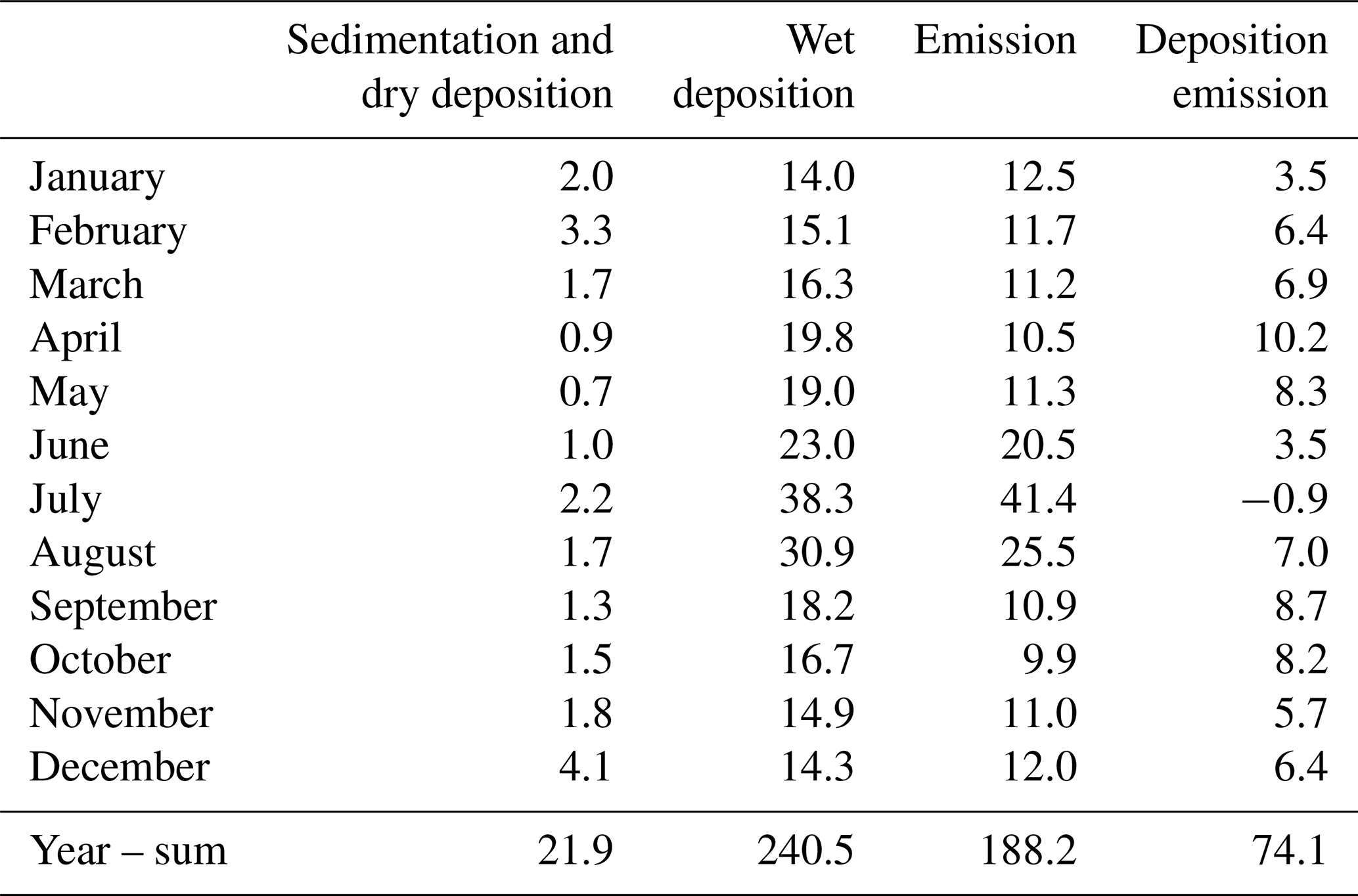
The removal process in ECHAM6.3-HAM2.3 is split between sedimentation, dry deposition and wet deposition. The sedimentation process describes the removal by gravitational settling and is applied only to accumulation- and coarse-mode particles. In the model, dry deposition is due to turbulent mixing and affects all but the nucleation mode particles. In the wet deposition scheme, particles are removed as activated aerosol only if the cloud is precipitating. Additionally, below-cloud scavenging is applied. For more details on the removal processes in ECHAM-HAM, see Zhang et al. (2012). Monthly and yearly mean values of BC emissions and deposition fluxes computed by ECHAM-HAM for the Arctic are given in Table 2. Wet deposition accounts for over 90 % of the BC removal and is therefore a crucial impact factor in the Arctic BC burden.
The modeled spatial aerosol distribution affects the climate simulations through interactions with radiation and clouds. A lookup table with precalculated Mie parameters is used to dynamically determine the particle optical properties, considering their size, composition and water content (Stier et al., 2005; Zhang et al., 2012). The description of cloud microphysics in ECHAM6.3-HAM2.3 is based on the two-moment scheme of Lohmann et al. (2008), which allows us to account for the impact of modeled aerosol populations on the number concentrations of cloud condensation nuclei and ice nucleating particles. Particles can collide with droplets and ice particles after they have formed. For further details on the model system, we refer to Stier et al. (2005) and Zhang et al. (2012).
2.2 Emission inventories
While here we focus on BC, the details on the emissions of other aerosol species can be found in Zhang et al. (2012). BC is emitted only in the hydrophobic Aitken mode with a median radius of rdry=30 nm and can grow into the bigger modes by aging and coagulation. It can also become hydrophilic by getting coated with sulfate. In this study, we use and compare four different emission setups, which are built from different emission data sets as described in the following.
We use the emissions developed for the Atmospheric Chemistry and Climate Model Intercomparison Project (ACCMIP) as described by van Vuuren et al. (2011). The data have a horizontal resolution and contain anthropogenic and biomass burning emissions that do not differ between years. The ACCMIP emission inventory is available with historic emissions until the year 2000 and for four different development scenarios linked to the Representative Concentrations Pathways (RCPs) for all later years (2000–2100; Lamarque et al., 2010). The anthropogenic emissions remain constant throughout the year. The biomass burning emissions vary monthly over the course of 1 year but are only scaled by a factor between the years and do not differ in their location. In this study, we only use year 2000 emissions.
The global emission data set created for Evaluating the Climate and Air Quality Impacts of Short-lived Pollutants (ECLIPSE), version 5a, by Klimont et al. (2017) includes only anthropogenic emissions. The horizontal resolution is . Historic emissions are available until 2010, and projections of different industrial development scenarios afterwards are linked to the RCPs. Unlike the ACCMIP emission data set, the anthropogenic emissions seasonally vary for the different sectors, and they also include emissions from gas flaring. However, gas flaring emissions from northern Russia have been considered to be difficult to measure and therefore uncertain and possibly too low in current emission inventories (Stohl et al., 2013).
To address the importance of local emissions, we use the anthropogenic BC emission data set for Russian BC, described in Huang et al. (2015). It is available for the year 2010 and originally comes in a horizontal resolution but is interpolated here to model resolution of T63 (approximately 1.8∘). Since the data set is limited to the area of Russia, we combine it with the ECLIPSE emission data. The Russian emissions are distributed between the different months with the monthly patterns of ECLIPSE. The emissions of Russian gas flaring are more than 40 % higher than those in ECLIPSE, resulting partly from a high conversion factor estimated for the fossil fuels found in Russia (Huang et al., 2015). It represents a reasonable yet high estimate of local emissions and is used as the reference setup. When compared, the ECLIPSE and Huang et al. (2015) emissions span an uncertainty range concerning gas flaring emissions.
GFAS (Global Fire Assimilation System) is a data set of biomass burning emissions. The strength of the emissions is scaled to the fire radiative power as observed by the MODIS instruments aboard NASA's Aqua and Terra satellites (Kaiser et al., 2012). This allows for a representation of real-time fires in ECHAM-HAM with daily changing emissions and enables it to reproduce the biomass burning plumes, which are regularly observed in the Arctic during spring and summer months. This covers natural fire events as well as those caused by anthropogenic activities. In ECHAM-HAM the biomass burning emissions are injected into the boundary layer regardless of the actual injection height provided by GFAS, which is usually reasonable for most small and moderate boreal fires, while the injection height can be underestimated for specific events with high fire radiative power (Sofiev et al., 2009). In previous works with ECHAM-HAM, GFAS emissions were often used with an emission factor of 3.4, as proposed by Kaiser et al. (2012). In an early setup, this led to a strong overestimation in BC concentrations in comparison to ground-based and airborne observations at mid-latitudes and high latitudes; it was therefore discarded.
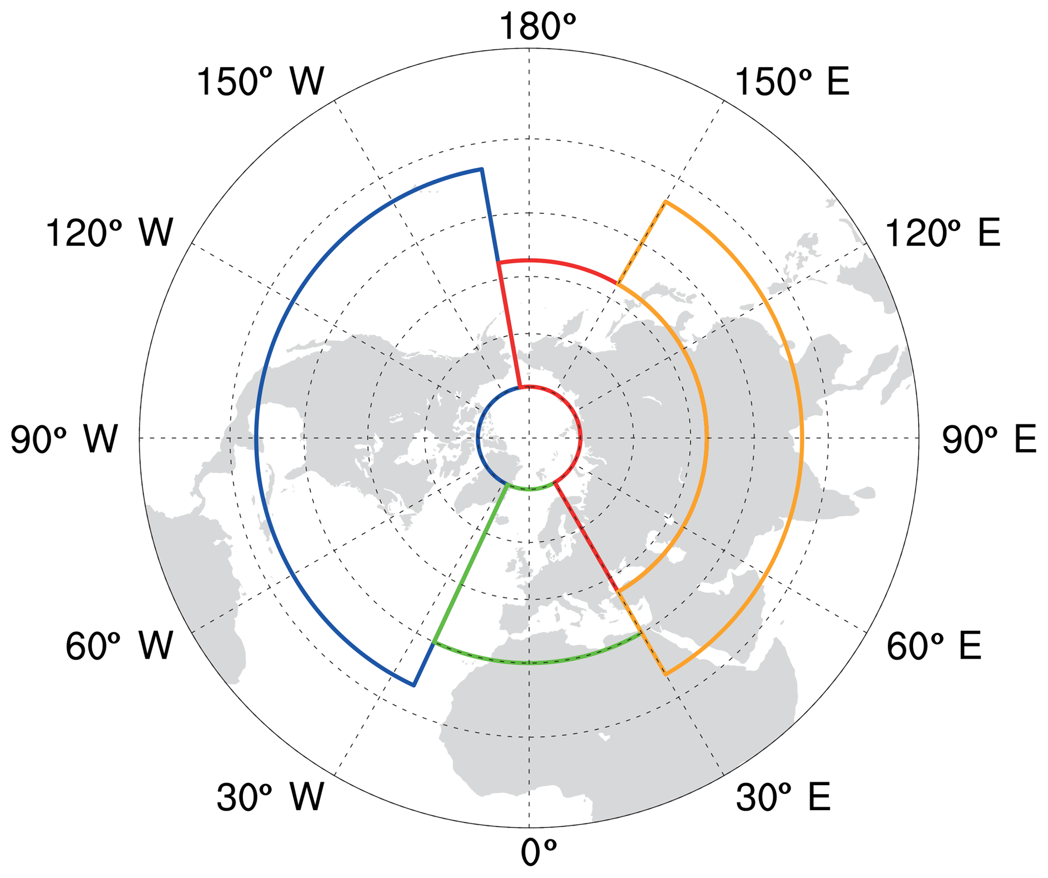
Figure 1Regions indicate the area used for averaging presented in Table 3. North America is in blue, Europe is in green, Russia is in red and central Asia is in orange.
Table 2Arctic BC budget averaged for the years 2005–2015 (in kt month−1) for BCRUS.
2.3 Experimental setup
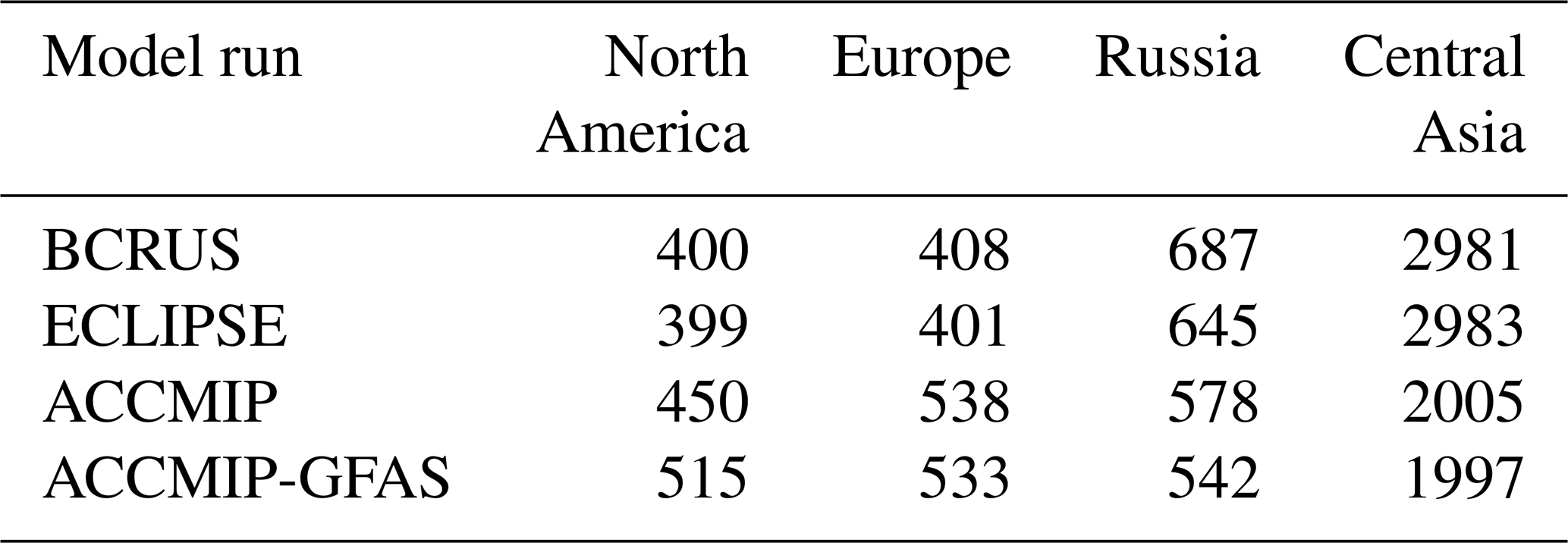
We run ECHAM6.3-HAM2.3 at T63 horizontal resolution (approximately 1.8∘), with 47 vertical layers. The model is driven with ERA-Interim reanalysis data and prescribed sea surface temperature (SST) as well as sea-ice concentrations (SIC). The model simulations cover the 1-year period 2005–2015, with a spin-up period of 3 months. One run is extended to June 2017 in order to include the period of a recent aircraft campaign. In total four model runs are realized, each with a different combination of emission data sets as described in the following. The time-averaged land emissions of BC from each setup are presented for different geographical regions in Table 3 (see Fig. 1 for location).
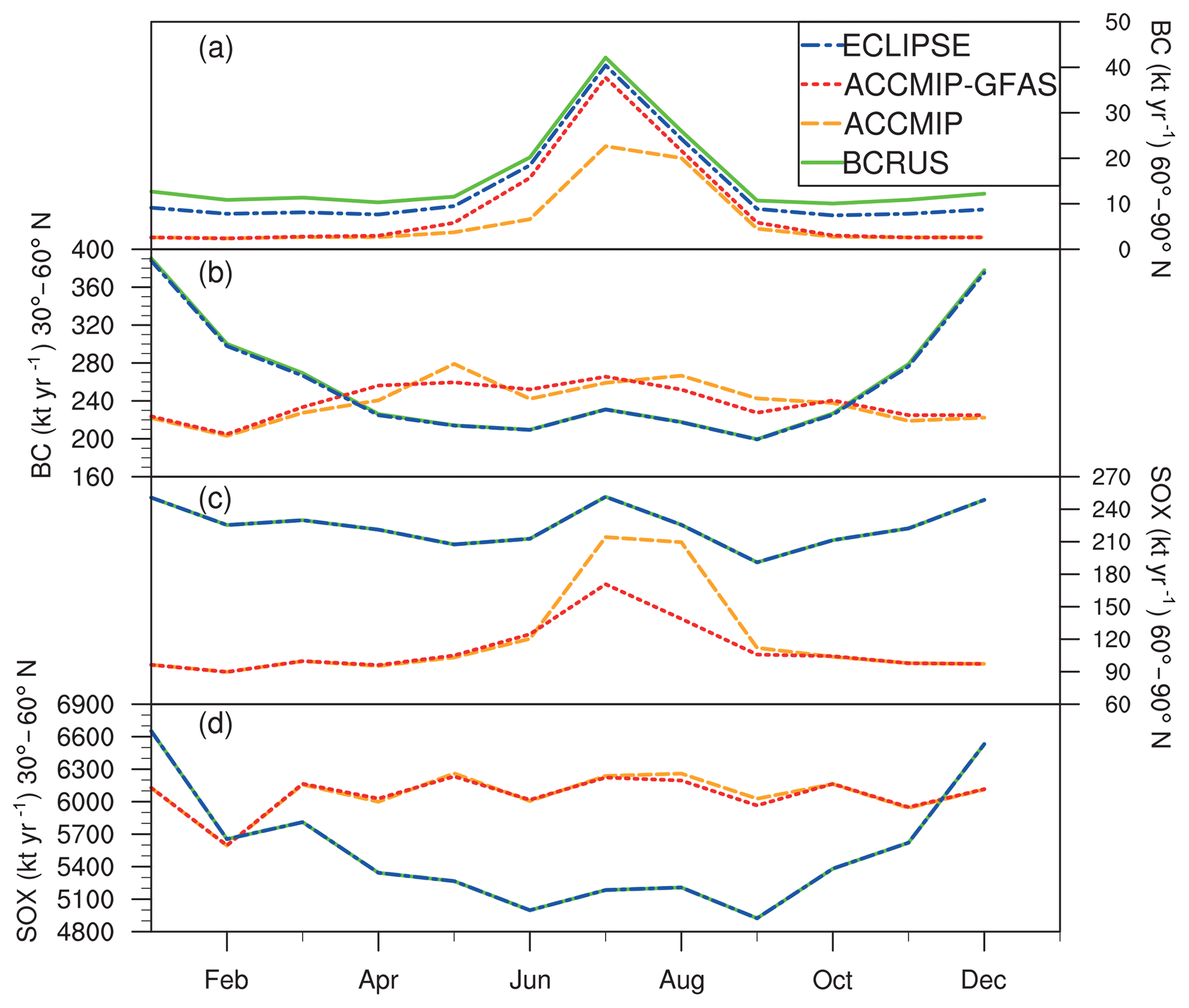
Figure 2Multi-year monthly mean emissions of (a, b) BC and (c, d) SOX (SO2 plus SO4) for the years 2005–2015. Values are integrated over the latitude band between 60 and 90∘ N and between 30 and 60∘ N.
For the first run we use the historical year 2000 ACCMIP emissions throughout the whole simulation period. Hereafter, this run is referred to as ACCMIP. ACCMIP emission data are still widely used for model experiments, in some cases using the RCPs (Lund et al., 2018), or fixed for the year 2000 (Sand et al., 2017). This simplification is a common approach to reduce degrees of freedom and control boundary conditions in non-transient climate studies. ACCMIP is the only run that does not use the daily updated GFAS emissions for biomass burning and can therefore not be expected to reproduce actual biomass burning events. Therefore, it can serve as a reference run needed to estimate the uncertainty that is related to the representation of biomass burning emission. The resulting monthly BC for the latitude bands of 30–60 and 60–90∘ N can be seen in Fig. 2. Sulfate is important for the aging and wet removal of BC; therefore the SO2 plus sulfate (SOx) emissions are given as well. It is the run with the highest European emissions, at 538 kt yr−1, and low central Asian emissions (see Table 3). The anthropogenic ACCMIP emissions are higher in Europe than for the other data sets used in this study because recent changes in air quality regulations led to lower emissions there in the period examined (considered until 2011). In Southeast Asia, they are, however, smaller, since the Asian economy has strongly grown since 2000, and with it the air pollutant emissions have also grown.
The second run, called ACCMIP-GFAS, combines the biomass burning emissions of GFAS with the year 2000 ACCMIP emissions from anthropogenic sources (orange line in Fig. 2). This run also does not account for changes in anthropogenic emissions but considers the day-to-day variability in wildfires. Together with a setup described in the following, it can be used to assess the range of uncertainty in anthropogenic emissions. This run has the highest average BC emissions in North America, at 515 kt yr−1, and the lowest central Asian emissions, at 1997 kt yr−1.
In the third run, we use the ECLIPSE RCP4.5 emission data combined with GFAS emission. It is referred to as ECLIPSE hereafter (blue line in Fig. 2). This run has the highest BC emissions in central Asia, with about 1.5 times the emissions of the ACCMIP runs (see Table 3).
The fourth run, which is referred to as BCRUS, uses the updated spatially highly resolved BC emissions from Huang et al. (2015), replacing and updating only the anthropogenic BC emissions in Russia. Elsewhere the emissions are the same as in the ECLIPSE run. This way, the BC sources are supposed to represent a high estimate, addressing the possibility of underestimation in the global data sets, in particular with respect to gas flaring. For other species, most notably SOX, the runs BCRUS and ECLIPSE do not differ (see green lines in Fig. 2).
BCRUS is chosen as the reference run, since it uses the most up-to-date data and is therefore assumed to be the best estimate. In BCRUS the BC emissions north of 60∘ N on land are even higher than over the oceans compared with the other data sets, at 172 and 7 kt yr−1, respectively.

Figure 3Maps of annual mean BC emissions for the years 2005–2015. (a) Absolute values are given for BCRUS. Difference between (b) the ACCMIP-GFAS and BCRUS results, (c) the ECLIPSE and BCRUS results, and (d) between the ACCMIP and ACCMIP-GFAS results.
Figure 3a shows the emissions of BC for the reference run BCRUS. The highest emissions north of 30∘ N are found in the industrial regions of East Asia, Europe and northeastern America as well as in gas and oil extraction areas in North America and northern Russia. The anthropogenic emissions in the sparsely populated northern Canadian and Alaskan regions are much lower than those of the densely populated European region. Additionally, the aforementioned gas flaring emissions in Russia are assumed to be higher than in northern North America. The transport efficiency from the East Asian sources to the Arctic is comparably low, but the high emissions in this region makes it important for long-range transport to the Arctic upper troposphere (Ikeda et al., 2017).
Figure 3b and c show the difference in BC emissions for the ACCMIP-GFAS and ECLIPSE runs compared with the BCRUS setup, respectively. BC emissions from ACCMIP-GFAS are higher than those of BCRUS in North America, Europe, western Russia and Japan. They are, however, lower in northern Russia by more than 3500 and China by more than 2800 . In northern Russia and China, however, ACCMIP-GFAS emissions of BC are locally over 3500 and 2800 lower, respectively. Figure 3c shows the difference between ECLIPSE and BCRUS. There are only differences in Russia, as expected. The ECLIPSE emissions are smaller than the BCRUS emissions because of newer information about additional sources. Among other sources, higher values are mainly due to gas flaring emissions. Figure 3d shows the difference in BC emissions between the runs ACCMIP and ACCMIP-GFAS that results from their difference in the biomass burning representation discussed above. ACCMIP shows higher emissions in Europe and Russia, while the emissions of ACCMIP-GFAS are higher in North America. The totals of BC emissions are summarized in Table 3.
2.4 Calculation of direct aerosol radiative effects of BC
For diagnostic output, the instantaneous radiative impact of all aerosol types is calculated in ECHAM-HAM by calling the radiation routine twice: once considering the interaction between aerosol particles and radiation and once without any aerosol. The difference between these two calls is then considered to be the direct aerosol radiative effect (DRE), which is free of any rapid adjustment (semi-direct effects).
To calculate the DRE by BC, the ACCMIP-GFAS and BCRUS runs were repeated, leaving BC out in the computation of radiative fluxes. For this, BC was skipped in the calculation of the complex radiative index and the radiatively active number of particles, while the wet radius of respective aerosol modes was not adjusted further. The DRE of BC is then derived from the difference of these two runs to their original setup. Note that with this method, the estimate includes the semi-direct effect of BC, which is small in the large-scale average, since positive and negative effects cancel each other out, and is not statically significant in the Arctic (Tegen and Heinold, 2018). The DRE of BC is studied for the sub-period 2005–2009.
The aerosol transport and radiation simulations in this study consider the reduction of snow albedo due to deposited BC. The BC-in-snow albedo effect is parameterized in terms of a lookup table based on a single-layer version of the Snow, Ice and Aerosol Radiation (SNICAR) model from Flanner et al. (2007). The scheme was first implemented in the earth-system model version of ECHAM6 by Engels (2016) and has become available recently in ECHAM6.3-HAM2.3 (Gilgen et al., 2018). It accounts for the BC concentration within in the uppermost 2 cm of snow. Input parameters are the snow precipitation, the sedimentation, dry deposition and wet removal of BC as well as on snowmelt and glacier runoff, the latter of which leading to an enrichment of BC in the remaining snow layer. The BC-in-snow albedo effect is computed for solar radiation only because the albedo is only used for shortwave (solar near-infrared and visible) wavelengths in the model. The effect in the terrestrial spectrum is very small and can be neglected for the atmosphere. A feature not considered so far is the impact of BC deposition on bare sea ice. This, however, is expected to be negligible, since the spatial extent of sea ice without snow cover is small (Gilgen et al., 2018). In this study, the parameterization is only used for diagnostics of the BC-in-snow albedo effect without any feedback on the model dynamics.

Figure 4Geographic regions of Arctic aircraft campaigns. The data of these are used for model evaluation: HIPPO in blue, ACLOUD and PAMARCMiP-2017 in green, ACCESS in red, and ARCTAS in orange. Black triangles show the location of stations with BC surface measurements.
Table 3Area-weighted totals of BC emissions from anthropogenic sources and biomass burning fires for the main source regions (as shown in Fig. 1) averaged for the years 2005–2015 (in kt yr−1).
2.5 Observations
2.5.1 Near-surface BC concentrations
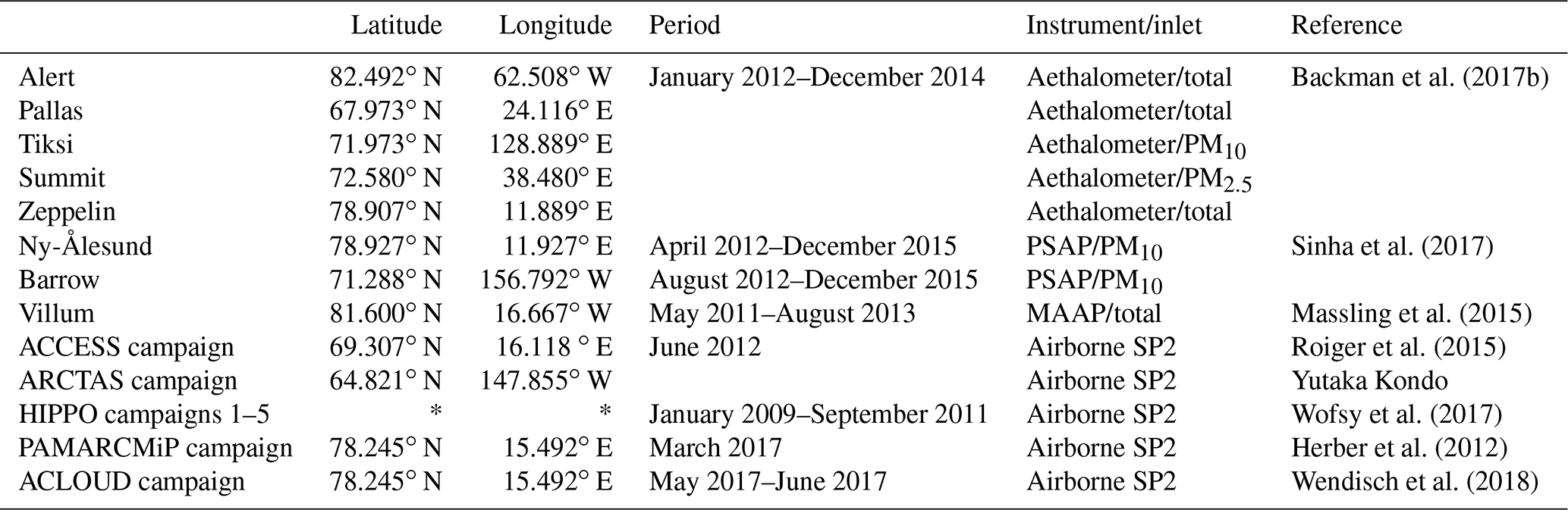
Near-surface BC concentrations are taken from different measurement sites around the Arctic, shown on the map in Fig. 4 as triangles. These sites utilize different measurement principles providing BC concentrations that differ by definition. The measurement principles, measurement period and the location of the measurements are summarized in Table 4.
At five of these sites light absorption was measured with aethalometers. Of those five stations, Alert and Summit measured at 467, 525 and 637 nm; Zeppelin Station measured at 525 nm only; and Tiksi and Pallas measured at 637 nm only. From the light absorption, equivalent black carbon (eBC) concentrations were calculated using different mass absorption coefficients (MACs) depending on the wavelengths. For the stations where measurements at 525 nm were available, 9.8 m2 g−1 was used for aged Arctic BC at 550 nm (from Zanatta et al., 2018). Zanatta et al. (2018) give an uncertainty of the MAC value of ±1.68 m2 g−1. This implies an uncertainty range of approximately −20 % to +15 % for the observed BC concentrations. For the stations where the light absorption was only available at 637 nm, a MAC of 8.5 m2 g−1 for Scandinavian BC was used at this wavelength correspondingly (Zanatta et al., 2016). The data were processed as described in Backman et al. (2017a) to reduce noise and lower the detection limit, which is important for the Arctic, since concentrations tend to be about 1 order of magnitude lower than at mid-latitudes outside of Arctic haze season. We use the variable collection time data from Backman et al. (2017b), which covers January 2012 until December 2014. The sites are Alert in Nunavut, Canada; Pallas in Finland; Tiksi in Sakha, Russia; Zeppelin Station in Svalbard, Norway; and Summit in Greenland, Denmark.
BC concentration data measured with a continuous soot-monitoring system (COSMOS), which removes volatile aerosol compounds, are available for Ny-Ålesund, Svalbard, Norway, and Barrow, Alaska, USA, for the period from 1 April 2012 to 31 December 2015 and 12 August 2012 to 31 December 2015, respectively. The data collection and the retrieval of BC mass concentrations using a MAC of 8.73 m2 g−1 at 565 nm are described in Sinha et al. (2017).
In addition, we use measurements of eBC concentration at the Villum Research Station in northern Greenland that were performed with a multi-angle absorption photometer (MAAP). We use daily averaged data from 14 May 2011 to 23 August 2013. Further information on data sampling and processing can be found in Massling et al. (2015).
For Alaska we use filter-collected BC data acquired by the Interagency Monitoring of Protected Visual Environments (IMPROVE) aerosol network. The thermal protocol used to process the measurements is described in Chow et al. (2007). We use data from the sites Tuxedni, Trapper Creek, Denali National Park (NP) and Gates of the Arctic NP.
2.5.2 Aircraft campaigns
The correct representation of the modeled aerosol vertical distribution is a key prerequisite for estimating the aerosol radiative impact (Samset et al., 2013). For this reason, we collected BC measurements from five Arctic airborne campaigns. During all flights, the mass concentration of refractory black carbon (rBC) was quantified by means of the single particle soot photometer (SP2), which ensures the high time resolution and high sensitivity required in airborne observations.
The HIPPO (HIAPER Pole-to-Pole Observation) campaign consists of five deployments by the National Science Foundation (NSF; data set – Wofsy et al., 2017, version 1): HIPPO-1 (9 to 23 January 2009), HIPPO-2 (31 October to 22 November 2009), HIPPO-3 (24 March to 16 April 2010), HIPPO-4 (14 June to 11 July 2011) and HIPPO-5 (9 August to 8 September 2011). Flights included Northern Hemisphere high latitudes over North America, the Pacific Ocean and the Bering Sea. BC particles were measured with an SP2. The aircraft used was the NSF/National Center for Atmospheric Research (NCAR) Gulfstream-V (GV).
The BC data from NASA's campaign ARCTAS (Arctic Research of the Composition of the Troposphere from Aircraft and Satellites) were collected in two deployments, spring (April 2008) and summer (June–July 2008), over North America and the American Arctic. The mission design and execution are described in Jacob et al. (2010) (data set – SP2_DC8; https://www-air.larc.nasa.gov/cgi-bin/ArcView/arctas/, last access: 2 July 2018).
The summer campaign of ACCESS (Arctic Climate Change, Economy and Society) in July 2012 took place over Scandinavia and the European Arctic (Roiger et al., 2015). The BC mass concentration was derived from measurements of a SP2 aboard the Falcon aircraft of the DLR (Deutsches Zentrum für Luft und Raumfahrt).
Another set of airborne measurements was collected from the 2017 PAMARCMiP (Polar Airborne Measurements and Arctic Regional Climate Model Simulation Project) campaign (Herber et al., 2012). The selected flight took place in March and was based in Longyearbyen, Spitzbergen, Norway, and made use of the Polar 5 aircraft of the Alfred Wegener Institute (AWI).
Also based in Ny-Ålesund was the ACLOUD (Arctic CLoud and Observations Using airborne measurements during polar Day) campaign, with measurements from 22 May to 28 June 2017 (Wendisch et al., 2018). Again, the BC concentrations were measured with an SP2 aboard the AWI Polar 5 aircraft.
The range of flight tracks of the aircraft campaigns used in this study are mapped in Fig. 4 as colored boxes, with HIPPO in blue, ACCESS in red, ARCTAS in orange, and the combination of ACLOUD and PAMARCMiP-2017 in green. The most western, eastern, southern and northern coordinates at which the aircraft took measurements form the edges of the boxes, with measurements south of 60∘ N not being considered. An overview of instruments and dates is given in Table 4. Even though aircraft campaigns can only give information within a short time window, the combination of different campaigns allows us to cover the almost entire year except for December, February, September and October, the months for which no aircraft data are available.
The comparison between a coarsely resolved model and aircraft measurements is challenging because of many factors. Any observed feature of subscale lifetime or spatial extend will be missed or at least underestimated by a model that is designed to estimate climate-relevant effects over multiple years. Schutgens et al. (2016) suggest either spatio-temporal averaging of both measurements and spacial interpolated model data or increasing the model resolutions to achieve the best agreement. Lund et al. (2018) show that using only monthly mean model output introduces significant biases.
In this study, we sample from the model's 12-hourly output for each measurement point during one campaign before averaging to one vertical profile, without prior interpolation.
In order to investigate the uncertainty range in the BC burden and its direct radiative impact, which results from the uncertainty in emissions, different simulations with the aerosol-climate model ECHAM6.3-HAM2.3 using four emission configurations are performed and compared as outlined in Sect. 2.3.
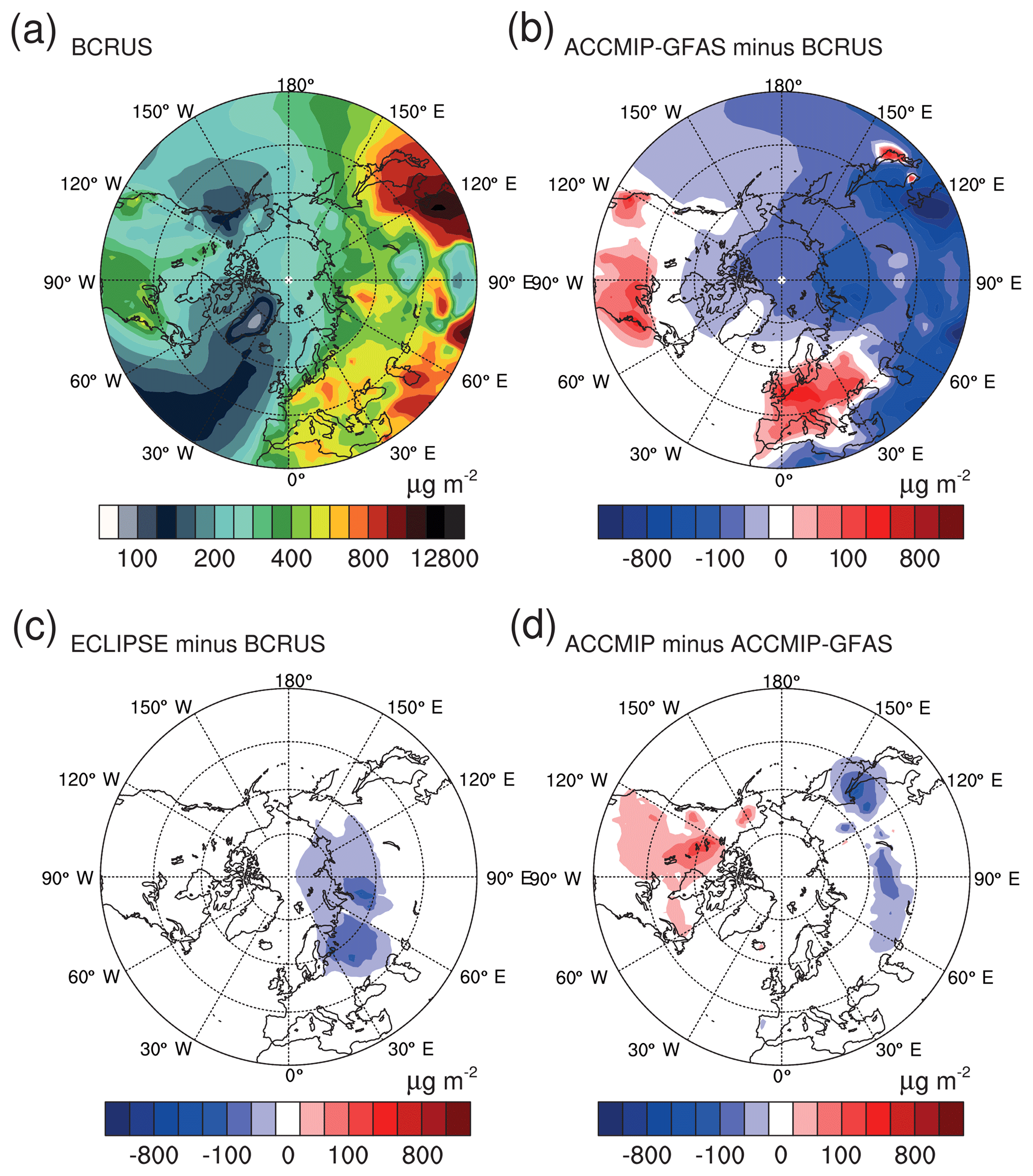
Figure 5Contour plot showing the modeled atmospheric BC burden averaged over the simulation period (2005–2015). (a) Absolute values from the BCRUS setup, which is used as the reference. (b, c) Differences of ACCMIP-GFAS and ECLIPSE to the BCRUS run, respectively. Blue colors indicate lower BC burden than in the BCRUS run, and red indicates higher BC burden. (d) Difference in modeled atmospheric BC burden between ACCMIP and ACCMIP-GFAS.
The atmospheric burden of BC averaged over the simulation period (2005–2015), which results from the different emission setups, is shown in Fig. 5. The distribution over the BC burden resulting from BCRUS (see Fig. 5a) is comparable to the distribution of the emissions in this run (see Fig. 3a). The northward transport results in a visible separation between the Eastern and Western Hemispheres in the BC burden in the northern part of 60∘ N, with higher values of 200 to 800 µg m−2 in the Eastern Hemisphere compared with values of 50 to 400 µg m−2 in the Western Hemisphere. This separation along the prime meridian is a result of higher anthropogenic emissions in the north of the Eastern Hemisphere, as discussed in Sect. 2.3. The area-weighted mean burden of BC north of 60∘ N of BCRUS is 254 µg m−2 in the multi-year annual average, which is the highest among the model runs used for this study. The highest values north of 60∘ N are located in the Russian gas flaring region, at over 560 µg m−2.
The causes and details, as well as differences between the runs, will be discussed in the following.
3.1 Recent economic changes
To estimate the range of anthropogenic emissions in currently widely used inventories, we compare the runs BCRUS and ACCMIP-GFAS. The ACCMIP run does not take recent economic changes into account, since emissions are fixed to the year 2000. BCRUS, on the other hand, is largely based on the ECLIPSE emissions that consider the economic development until 2015 and provide projections for the years after. Since both are combined with the biomass burning emissions from GFAS (which covers natural as well as human-caused fires), the differences in BC emissions are solely in the anthropogenic emissions (excluding human-caused grass and forest fires).
The use of fixed emissions in ACCMIP-GFAS causes a remarkable difference in the atmospheric burden of BC over the source regions compared with the reference run (see Fig. 5b). ACCMIP-GFAS does not catch the reduction in BC emissions over western countries and Japan due to the implementation of strict air quality legislation and the increased emission over China caused by its economic growth. The neglect of the recent economic evolution and mitigation policies results in an overall underestimation of the BC burden by 63 µg m−2 (25 %) within the 60–90∘ N latitudinal band. Over the Kara Sea, the result is an underestimation that exceeds 100 µg m−2; this is a region that has been considered to be a hotspot for the connection between Arctic sea-ice loss and changes in the large-scale atmospheric circulation with particular sensitivity (e.g., Petoukhov and Semenov, 2010).
3.2 Regional refinement
Higher, more realistic estimates of emissions for Arctic sources (e.g., gas flaring) have been discussed as a requirement for reproducing observations like locally high BC concentrations in snow (Eckhardt et al., 2017) as well as the layering and seasonality of Arctic aerosol concentration far from sources (Stohl et al., 2013). However, improving the regional accuracy of BC emissions in the Russian Arctic does not impact the modeled BC spatial distribution meaningfully outside of the Russian Arctic. As seen in the comparison of the runs BCRUS and ECLIPSE (Fig. 5c), the difference in the BC burden between BCRUS and ECLIPSE shows only differences visible in Russia, since the BC emissions differ only there (see Table 3 and Fig. 3). This results in an increase in the BC burden, mainly in the eastern Arctic, with up to 25 µg m−2 higher values over the Barents Sea and Kara Sea. The area-weighted annual averages north of 60∘ N differs by 11 µg m−2, with the higher BC burden being produced by BCRUS. However, stronger effects are found for BC near-surface concentrations as discussed below, due to the vicinity of the refined sources to the Arctic and the resulting transport at the lowest atmospheric levels.
3.3 Temporal variability in wildfire events
The atmospheric composition and, in particular, the BC loading are strongly influenced by wildfires, which have a strong spatio-temporal variability. The importance of considering actual biomass burning events is demonstrated by comparing the runs ACCMIP-GFAS and ACCMIP. While ACCMIP-GFAS accounts for real fire events derived from satellite retrievals, ACCMIP uses fixed fire emissions for the year 2000. The ACCMIP-GFAS BC emissions are higher than the ones of ACCMIP by 64.5 kt yr−1; this is mainly caused by North American emissions (see Fig. 3d).
The patterns of the BC burden of both runs are similar, with a higher burden over the western industrialized countries and a lower burden over China compared to BCRUS. The area-weighted average burden of BC estimated with ACCMIP is 186 µg m−2, which is 11 µg m−2 (6 %) less than ACCMIP-GFAS. A map of the differences in the annual average burden of BC due to the different representations of biomass burning emissions is shown in Fig. 5d. A clear pattern of a lower BC burden over southern Siberia and a higher burden over North America is visible. For the high Arctic, both runs produce a similar burden in the 11-year mean, with differences in the BC burden of less than 25 µg m−2. However, for short time periods, influenced by biomass burning events, the difference between the two runs can be dramatic, as shown below for comparisons of the BC mass concentration.
4.1 Near-surface BC mass concentration
Near-surface measurements of BC mass concentrations can help evaluate the capability of ECHAM-HAM to reproduce the distribution of BC in the Arctic atmosphere and hence reasonable estimates of the warming influence of absorbing aerosol. While the data are only representative of the lowest atmospheric layer, the long time series give robust information about this specific important climate forcer. The multi-year seasonality of near-surface BC is compared with observations in the Arctic, as is the temporal correlation, with a spatial emphasis. Each measurement point is compared with the nearest grid cell at the closest time step from the model. The medians are calculated after this sampling.
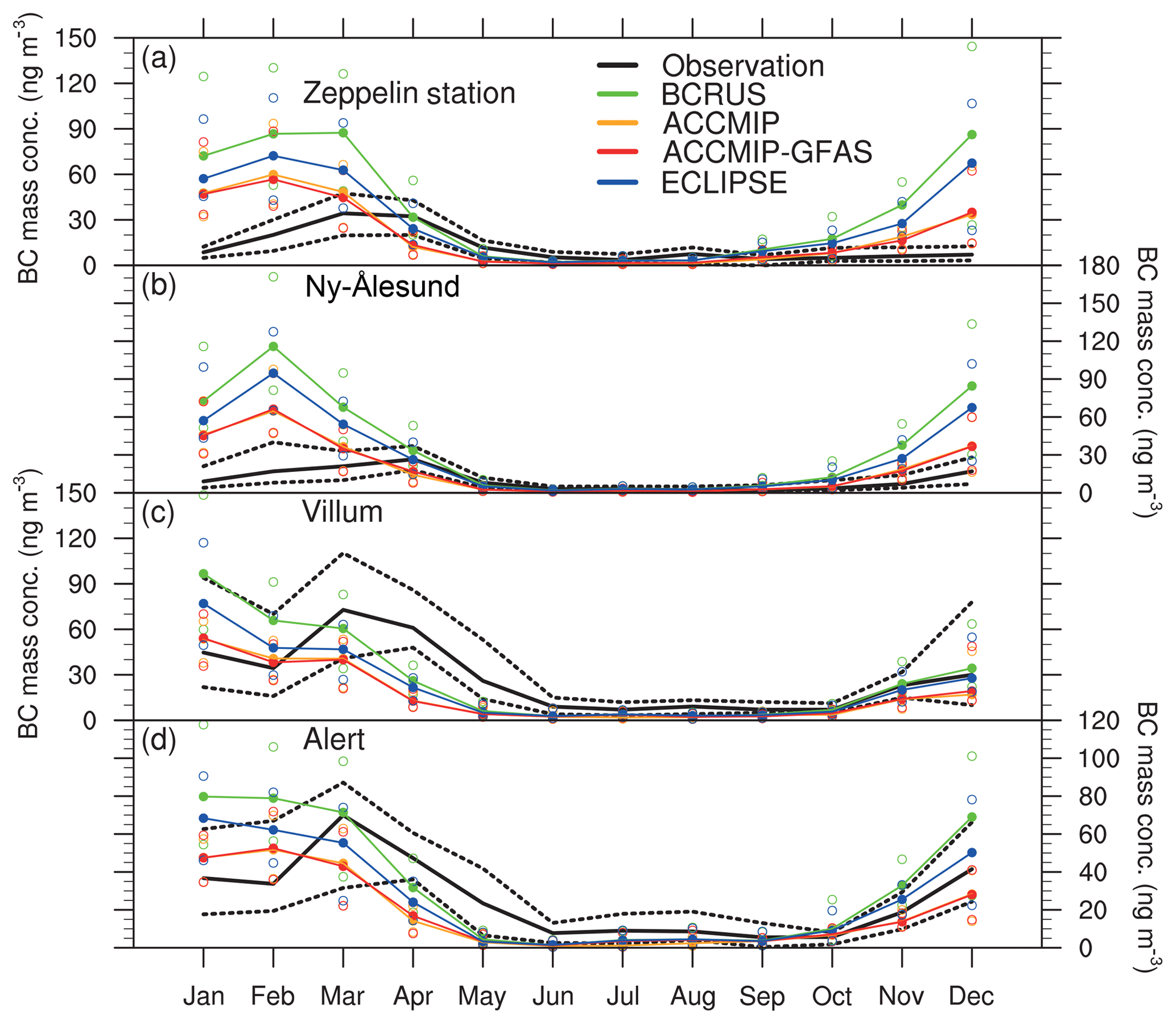
Figure 6Near-surface BC mass concentrations for Atlantic Arctic stations. Solid black line shows the multi-year monthly median BC mass concentration observed in (a) Zeppelin Station, (b) Ny-Ålesund, (c) Villum and (d) Alert. See Fig. 9 for the geographical locations. Dashed black line indicates the observed upper and lower quartiles. In color are the median different model runs with solid lines and filled circles, and the upper and lower quartiles run with empty circles.
Figures 6 through 8 each show the comparison of the observed and modeled monthly median mass concentration of near-surface BC for four available Arctic field sites averaged over multiple years. A list with detailed information on measurement period, instrumentation and data providers can be found in Table 4. The model is compared with the measurements in terms of how well the annual cycle is reproduced by comparing median BC mass concentration values and in terms of the ability to reproduce pollution events at the correct time by analyzing the Pearson correlation coefficients.
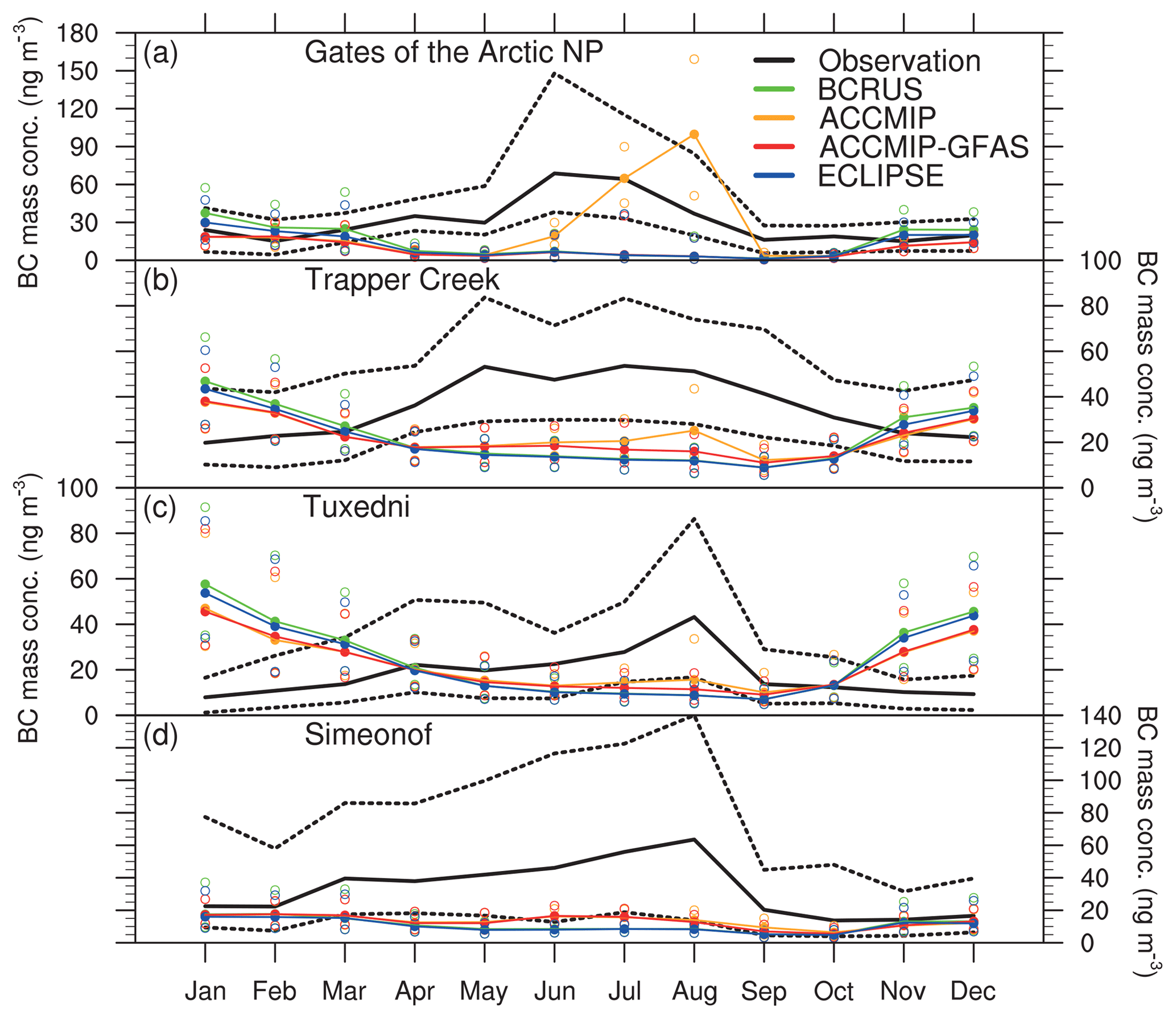
Figure 8As in Fig. 6 for the American Arctic stations of the IMPROVE network in Gates of the Arctic NP (a), Trapper Creek (b), Tuxedni (c) and Simeonof (d).
Of the stations used, Zeppelin Station and Ny-Ålesund are located in Svalbard. Alert and the Villum Research Station are both situated in the north of the Greenland ice sheet. The annual cycle of the BC concentration is shown in Fig. 6 in terms of the median, upper and lower quartiles in black; the different model runs are color coded. At all four stations, the maximum median BC mass concentration is observed in spring, at 36, 72 and 73 ng m−3 for Zeppelin Station, the Villum Research Station and Alert in March, respectively.
For Ny-Ålesund the highest concentrations are observed in April, with a median of 30 ng m−3. For all stations in Fig. 6 there is a minimum in summer, with less than 15 ng m−3 median BC concentrations in the near-surface air. At all four stations, the reference run BCRUS produces higher median concentrations in January than observed. The modeled BC mass concentrations are underestimated by the model at all of these stations except Ny-Ålesund, at least for some months. The model overestimates the BC concentrations in the beginning of the year at all stations. The overestimation is largest at Ny-Ålesund, with monthly median values of up to 120 ng m−3 for BCRUS, compared with the measured median of 20 ng m−3.
For Zeppelin Station and Ny-Ålesund, BC is also overestimated in November and December. Here, the model simulates monthly median values, each at 90 ng m−3, for December compared with measured medians of 10 and 20 ng m−3 for Zeppelin Station and Ny-Ålesund, respectively. It has to be noted that, in the model resolution, Zeppelin Station and Ny-Ålesund are in the same grid box. The difference in altitude is not taken into account from the model side; instead the lowest level above the modeled orography is chosen. Differences in the model results between the two stations, shown in Fig. 6, are only due to the different temporal availability of the measurements. Interestingly the model agrees slightly better with the observations at Zeppelin Station, which is more exposed to long-range transport, while Ny-Ålesund is often subject to a blocking situation that prevents mixing of air mass because of its respective location.
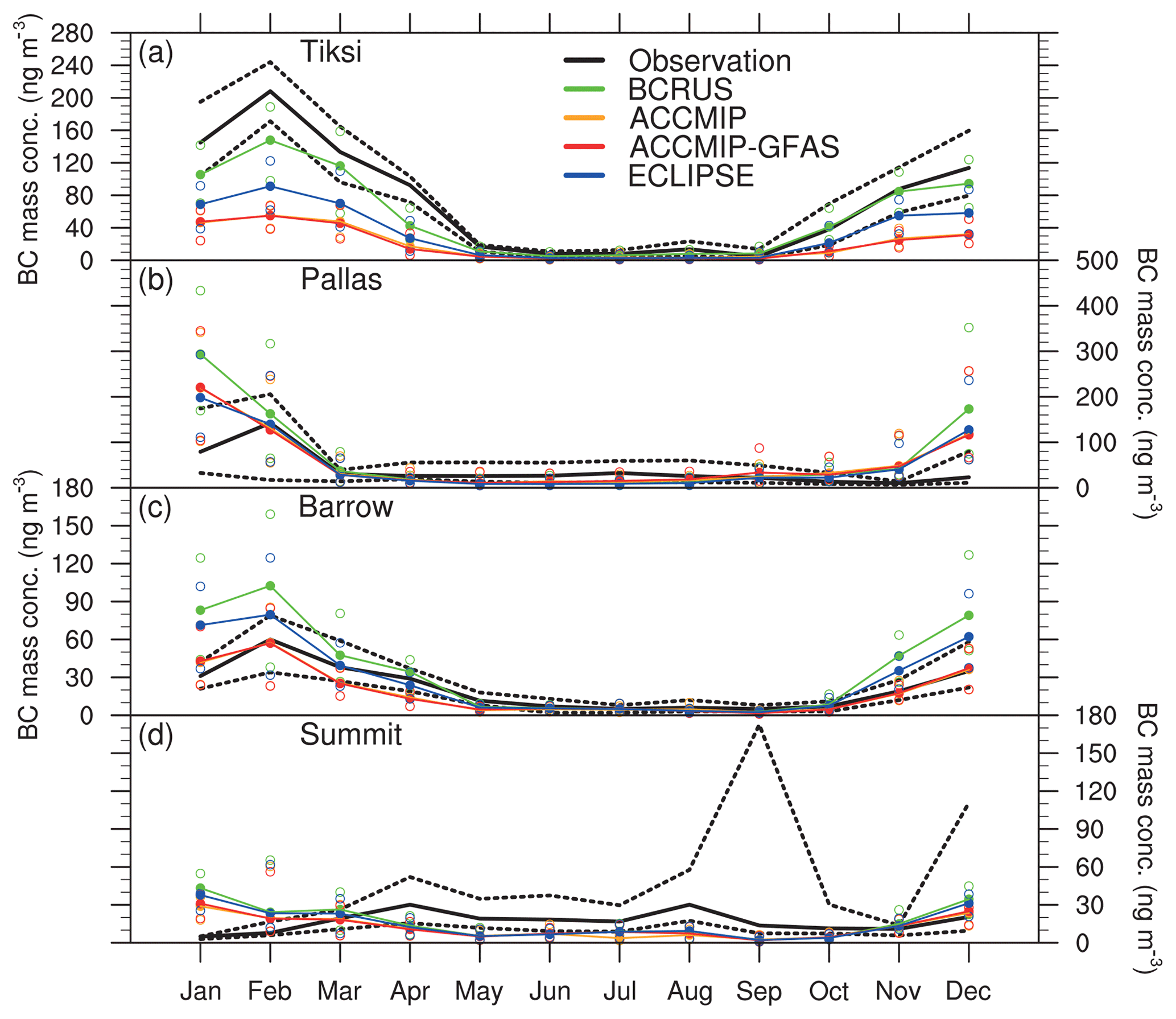
Figure 7 shows the second set of stations. Tiksi, Pallas and Utqiaġvik (Barrow) show the same annual cycle as the stations in Fig. 6, with high concentrations in winter and spring as well as minimum concentrations in summer. The model slightly underestimates BC at Tiksi in all months, with high concentrations of over 50 ng m−3. For Pallas and Utqiaġvik (Barrow) an overestimation by the model is found for January. Summit shows a different annual cycle in the observations, with the highest median BC mass concentrations of slightly more than 30 ng m−3 being observed in April and with slightly lower values in summer, and a minimum was observed for January. The model was neither able to reproduce this different annual cycle nor the peak in the quartiles during September and December that were observed. However, the amount of BC mass agrees well between model and measurements, with values generally below 30 ng m−3.
Results for four Alaskan stations of the IMPROVE network are shown in Fig. 8. There, the highest median BC concentrations are observed in the summer months, at 70 ng m−3 at Gates of the Arctic NP in June, 50 ng m−3 at Trapper Creek in July, and 40 and 60 ng m−3 at Tuxedni and Simeonof in August, respectively. The model noticeably fails to reproduce these summer maxima and instead produces the highest concentrations in January to March in a similar way as for the other Arctic stations. In Tuxedni, the simulated median concentration lies at 60 ng m−3, while the observed one is at 10 ng m−3. The Brooks Range spans through Alaska, from the Bering Sea in the west to the Beaufort Sea in the east, with multiple peaks of more than 2000 m a.s.l. Situated south of Brooks Range, the four stations are shielded from the Arctic. An underestimation of the orographic height in the coarsely resolved model could therefore be the reason for this misrepresentation.
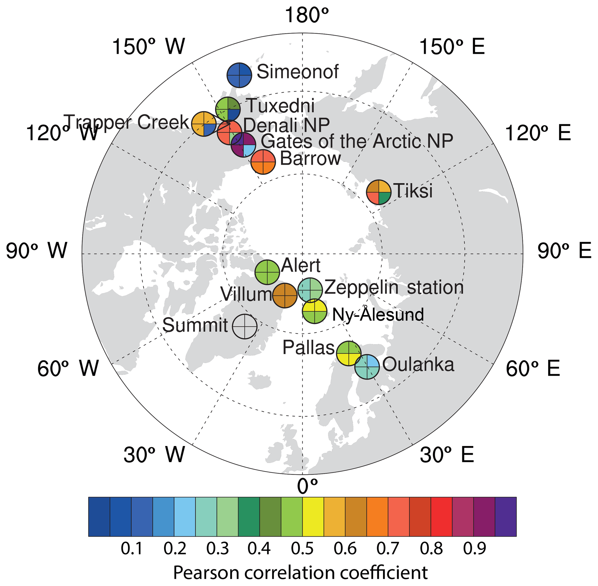
Figure 9Map showing the Arctic sites where the near-surface BC mass concentration was measured. Colors show the correlation coefficient between the measured and modeled daily averages. Correlation coefficients close to zero are not colored. Top right segment indicates the correlation coefficient for the BCRUS run. Clockwise are the ACCMIP, ACCMIP-GFAS and ECLIPSE runs. The label of Zeppelin Station is shifted to the north on the map for better visibility. The label of station Trapper Creek is shifted to the southeast.
The Pearson correlation coefficient between the collocated data of measured and modeled BC mass concentrations for all available aerosol stations in the Arctic region is shown in Fig. 9. Since pollution events in the Arctic can raise the BC concentrations to levels well above the background, the correlation coefficient is very sensitive to the model being able to reproduce the timing of pollution events. Therefore, this analysis complements the median and quartiles discussed above.
The top right segment of each circle shows the correlation coefficient between the BCRUS model run and the measurements. Following clockwise are the correlations for the runs ACCMIP, ACCMIP-GFAS and ECLIPSE. The circle for Summit is not filled, since there the correlation coefficients are negative albeit close to zero (−0.06 for BCRUS). The negative correlation corresponds to the opposite annual cycle of surface BC in the BCRUS model results compared with the observations as shown in Fig. 7. For all other stations, correlation coefficients are positive. Simeonof, on the Alaska Peninsula, shows a very weak correlation, with 0.09 for the different model runs. Tuxedni, on the southern coast of Alaska, also has a relatively low correlation coefficient of 0.44.
For the other Alaskan stations of the IMPROVE network, however, a correlation between observations and BCRUS model results is found that is robustly positive. Even for the stations where the annual cycle was not reproduced, the correct timing of short-term events leads to these positive correlation coefficients. Trapper Creek shows a correlation coefficient of 0.55, Denali NP of 0.72 and Gates of the Arctic NP of 0.94. ACCMIP clearly performs the worst of all experiments, with correlation coefficients 0.14, 0.31 and 0.20 for Trapper Creek, Denali NP and Gates of the Arctic NP, respectively, while the other runs do not differ strongly from each other. Taking the position and strength of actual biomass burning events into account is crucial for correctly reproducing the near-surface BC concentrations in Alaska.
The correlation coefficient at Oulanka is below 0.3 for all runs. This, however, is computed only on the basis of 3 months of measurements. The other European stations of Pallas, Ny-Ålesund and Zeppelin Station also show relatively low correlation coefficients of 0.45, 0.50 and 0.30 for BCRUS, respectively. The other runs behave similarly.
At the four northernmost stations, Tiksi, Utqiaġvik (Barrow), Alert and Villum Research Station, correlation coefficients of 0.55, 0.65, 0.60 and 0.60 are found for BCRUS, respectively. These four stations are located north of a big land mass and likely show a good correlation, since concentrations are drastically different when the wind either comes from the land or the Arctic Ocean. With the exception of Tiksi, the ACCMIP run does not produce considerably weaker correlations with the observations than the other runs. At Tiksi, the highest correlation coefficient is expected for BCRUS, since BCRUS comprises the most recent and detailed emissions specifically for Russia. At 0.56 compared with 0.71 (ACCMIP-GFAS) and 0.61 (ECLIPSE), the correlation is, however, the lowest.
4.2 Vertical distribution of BC
The BC mass mixing ratio from airborne measurements is a valuable source of information about the vertical distribution of BC. However, because of the logistical difficulties and high costs, the spatial and temporal coverage is quite sparse. The aircraft campaigns used in this study for model evaluation are described in detail in Sect. 2.5.2, their geographical operation area is presented in Fig. 4 and they are listed in Table 4. Each measurement point is compared with the nearest grid cell from the model, resulting in one average profile per campaign and run. We group the campaigns based on season, resulting in at least one profile per season, with better coverage during spring and summer, which have three and four campaigns, respectively.
4.2.1 Winter
For the winter months (December–January–February; DJF) only data from the HIPPO campaign are available, starting with the first deployment during January 2009. We consider only data points north of 60∘ N. The area covered by HIPPO is indicated by the blue box in Fig. 4. As shown in Fig. 10, observed BC mass mixing ratios were highest near the ground. Everything below 950 hPa is removed from the plot because of unrealistically high measured BC mass mixing ratios near the ground of over 450 ng kg−1 on average, which could not be reproduced by the model. Starting at 950 hPa the simulated profile of BCRUS is very similar to the observed vertical distribution. Model results and measurements show a decrease in BC with height, with the BCRUS run overestimating the BC mass mixing ratio above 900 hPa by a factor of about 2. The ECLIPSE run produces almost the same profile; however the runs ACCMIP and ACCMIP-GFAS produce lower values that, while still higher, are closer to the observed profile. Since the emission of BC for these runs is only lower in central Asia (see Table 3), this likely points toward an overestimation of the modeled transport to the Arctic, possibly caused by an underestimation of wet removal.
4.2.2 Spring
The observed and modeled profiles of BC mass mixing ratios from the ARCTAS spring campaign over the American Arctic (orange box in Fig. 4) in April 2008 can be found in Fig. 11a. Observations show high values near the ground, with a BC mass mixing ratio of over 40 ng kg−1, and a steep increase from there towards a pollution layer, with a maximum of almost 200 ng kg−1 at a 600 hPa height. BCRUS (in green) correctly places this layer but underestimates its strength. A second BC layer is centered at about a 400 hPa height, with the mixing ratio gradually decreasing above. All model runs including actual fire emissions are well able to capture the placement of the aerosol layer, while the magnitude is underestimated by a factor of up to 3. This could be caused by emissions that are too low in the source region with a correctly predicted transport or could just be an effect of the coarse resolution of the model, resulting in the emissions for the fire event being mixed over the grid boxes instead of being concentrated in a confined plume. In particular, small local fire plumes may be too strongly diluted when emitted into the model boundary layer. In addition, there is the possibility of a large sampling bias, with fire plumes being specifically probed during the campaign (Jacob et al., 2010). The other runs using GFAS produce similar results, with ECLIPSE and BCRUS performing the best. The ACCMIP run without daily fire emissions deviates most from the observations. This shows that this BC distribution was in fact largely caused by a biomass burning fire plume.
The averaged profile of the measured BC mass mixing ratio for the HIPPO-3 campaign over the Pacific in March–April 2010 is plotted in Fig. 11b. It shows observed mixing ratios of 20 ng kg−1 near the surface. There is a local minimum at a height of 880 hPa. The highest mass mixing ratio of BC is found at heights around 520 hPa. ECHAM-HAM is able to reproduce this profile well up to a height of about 650 hPa in all runs. From there the model underestimates the amount of BC up to the height of about 400 hPa. Above this, the model overestimates the amount of BC. The overestimation at uppermost levels is twice as high in the ECLIPSE and BCRUS model runs. They likely overestimate the long-range transport from Southeast Asian or Russian pollution sources. Close to the ground, BCRUS and ECLIPSE are better able to reproduce the observed mass mixing ratio.
The ACLOUD campaign took place around Svalbard in May and June 2017 and therefore represents late spring and early summer. As can be seen in Fig. 11c, the mixing ratio during the ACLOUD campaign was low, with observed mass mixing ratios of 4 to 5 ng kg−1 near the ground. A maximum with 14 ng kg−1 was observed at 800 hPa, above which the mass mixing ratio declined with increasing altitude. ECHAM-HAM reproduced this averaged profile relatively well, only placing the maximum too high at a height of 650 hPa, where the observations again decreased to 4 ng kg−1. This overshooting by ECHAM-HAM, at upper levels, is mainly found for the last flight on 16 June 2017 (not shown separately). This already hints to the tendency of ECHAM-HAM to overestimate upper-layer transport of aerosol in summer, as described in the text below. Note that for ACLOUD, only BCRUS results can be presented because of the timeliness of the measurements.
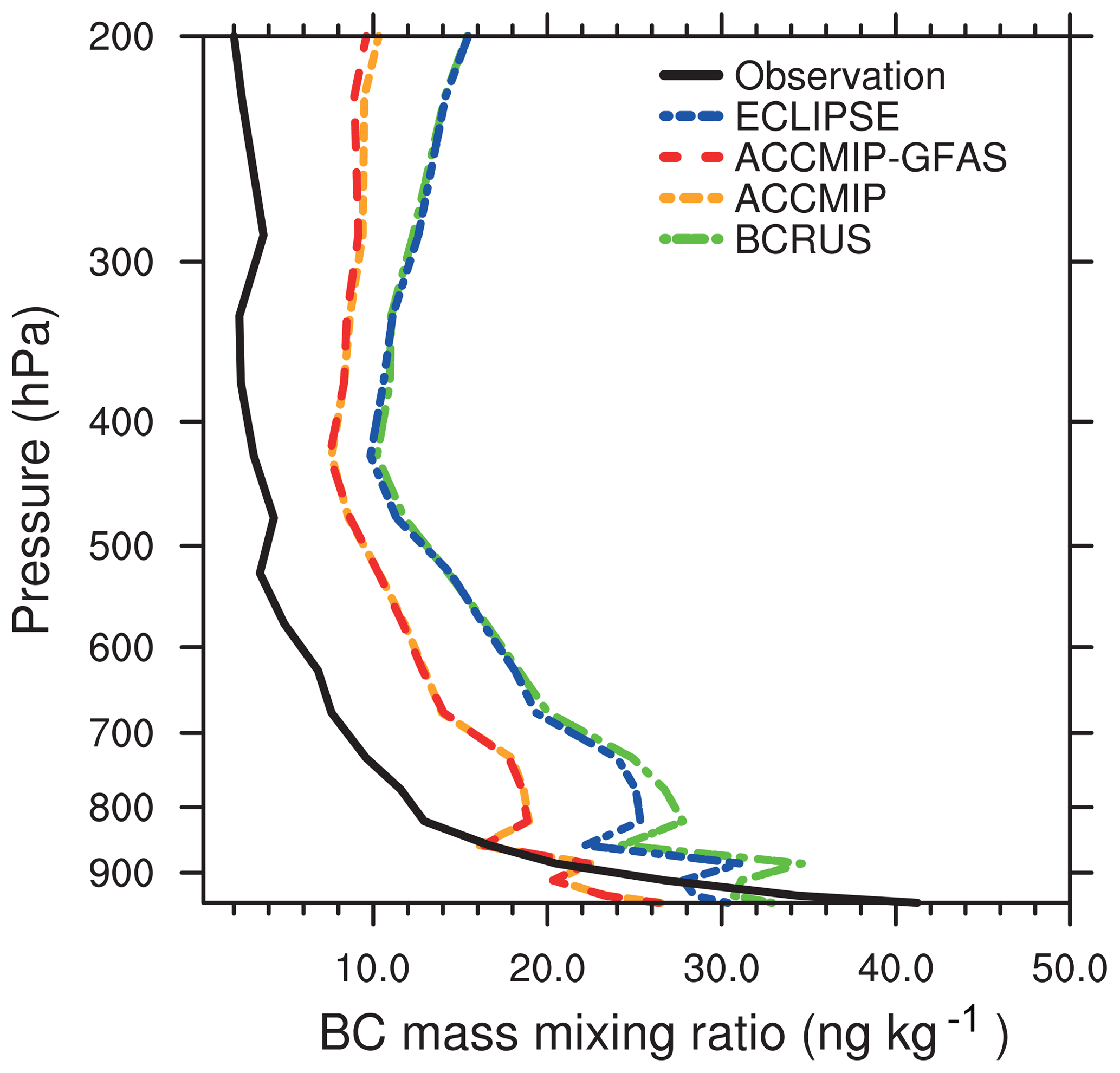
Figure 10Vertical profiles of BC mass mixing ratios from airborne in situ measurements during the flight campaign HIPPO-1 campaign in January 2009. The modeled BC mass mixing ratios were averaged over the vertical levels. The observations are shown in black, and the different model runs are color coded (see Sect. 4 for details).
4.2.3 Summer
Results for the comparison between the ARCTAS summer campaign over the American Arctic in June and July 2008 and the model results from ECHAM-HAM are shown in Fig. 12a. The averaged profile over the campaign shows an increase in the BC mass mixing ratio, with increasing height up to a maximum of 26 ng kg−1 at the 300 hPa level. As discussed by Matsui et al. (2011), air mass during this campaign was influenced by biomass burning in eastern Russia. Most of the BC from these fires, however, was quickly removed from the atmosphere by wet depositions by heavy rain close to the source region (Matsui et al., 2011). BCRUS produced a similar profile, with BC mass mixing ratio values very close to the observations up to 700 hPa height. Above this level, the model overestimates the amount of BC. This points toward a misrepresentation in the wet removal process or possibly vertical mixing or uplift of fire aerosol that is too efficient in the model. ACCMIP strongly differs from the other runs and observations, producing much higher mixing ratios below 550 hPa height. Above 570 hPa the BC mass mixing ratios modeled by ACCMIP, however, are much closer to the observations. At this height, Matsui et al. (2011) found elevated values in measured CO, pointing toward an influence by biomass burning fires. ACCMIP agrees best with the measurements because the observed fires that lead to the overestimation in the other runs are not present in the run. In this way, it produces values that are similar to the observations where biomass burning aerosol was removed.
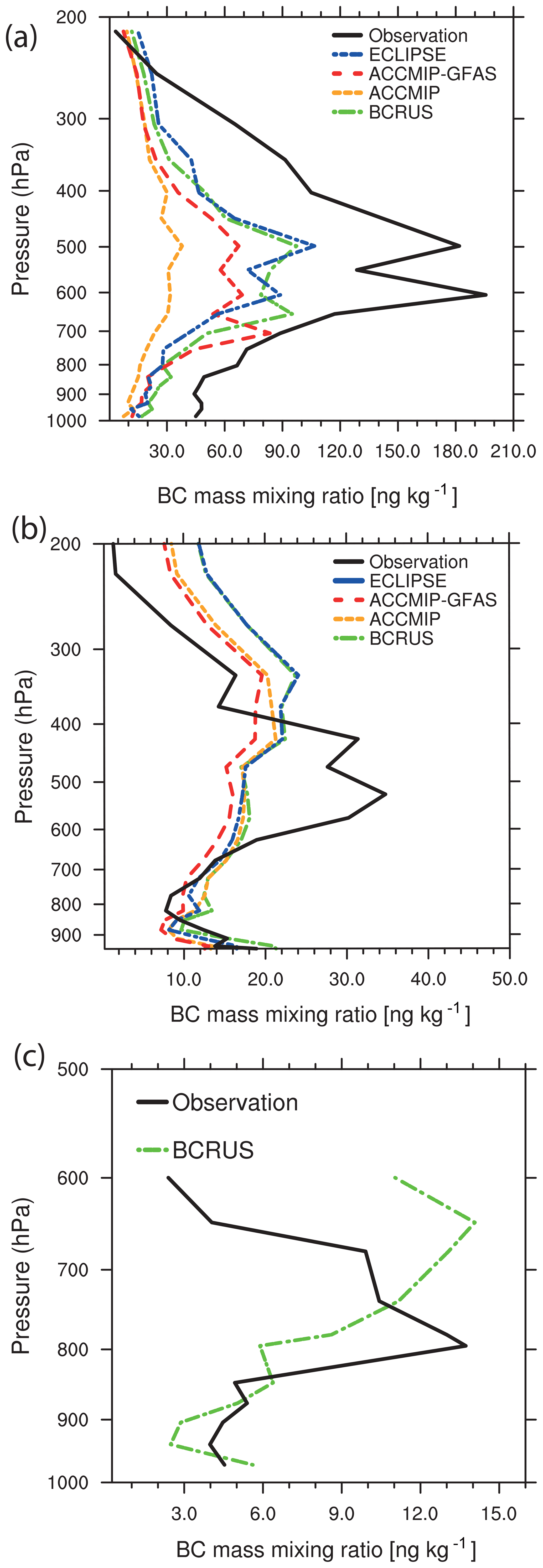
Figure 11As in Fig. 10, but with spring campaigns (March–April–May). (a) ARCTAS spring campaign in April 2008. (b) HIPPO-3 campaign in March–April 2010. (c) ACLOUD campaign in May–June 2017. Note that for year 2017, model results are only available from the BCRUS run.
Observations from HIPPO-4 (June–July 2011) and model results are compared in Fig. 12b. Modeled and observed mixing ratios are relatively low, with the highest observed BC mass mixing ratio at just above 19 ng kg−1. In BCRUS this maximum is found at 820 hPa; this is much lower than observed (620 hPa). The modeled vertical extent of this pollution layer is also thinner than observed. The major difference is BC amounts that are far too high between 500 and 200 hPa in the model results for all emission setups. Noteworthy is also the difference between the runs of ACCMIP and ACCMIP-GFAS, with ACCMIP performing better than the others runs in reproducing the pollution layer in the lower troposphere. The emissions from the actual fires in the GFAS emissions seem to not have reached the observed height but instead mostly remained below 800 hPa. The ACCMIP biomass burning emission coincidentally allowed ECHAM-HAM to reproduce a layer that is influenced by biomass burning in the same height as observed. The fact that all runs that use GFAS produce the same profile, while the only run without it produces a different profile, shows that the BC profile, at least up to a height of 300 hPa, is mainly caused by fire emissions.
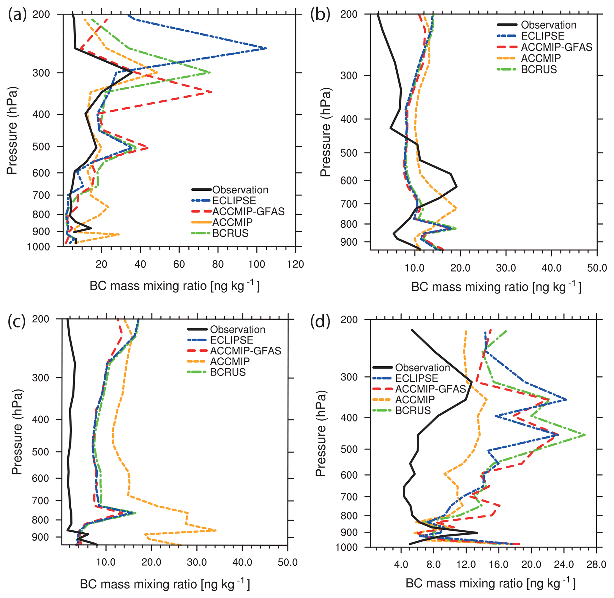
Figure 12As in Fig. 10, but for summer campaigns (June–July–August). (a) ARCTAS summer campaign in June–July 2008. (b) HIPPO-4 campaign in June–July 2011. (c) HIPPO-5 campaign in August–September 2011. (d) ACCESS campaign in June 2012.
The profile plot for HIPPO-5 (August–September 2011) shows low observed and modeled mass mixing ratios throughout the atmosphere (see Fig. 12c). The observations show the highest mass mixing ratio close to the surface at 9 ng kg−1 and a decrease towards 870 hPa to values just over 1 ng kg−1. The observed BC mass mixing ratio stays low at layers above. BCRUS produces lower BC mass mixing ratios near the surface and overestimates the amount of BC above 850 hPa. ACCMIP is the only run producing significantly different BC mass mixing ratios from the other runs, with strong overestimation throughout the profile and BC mixing ratios of up to 34 ng kg−1 at a height of 930 hPa. This strong overestimation is related to inappropriate biomass burning emissions in ACCMIP in this area.
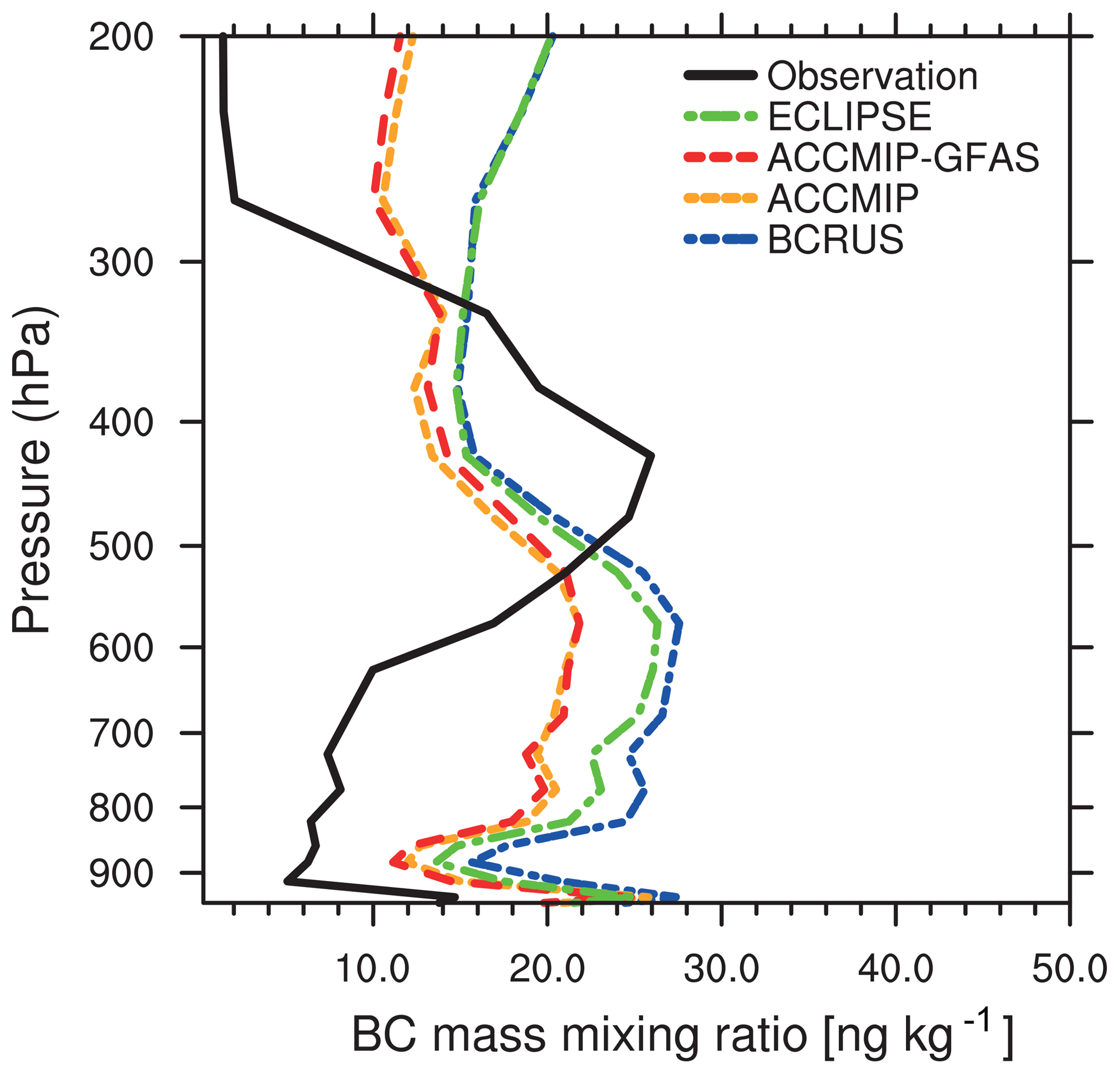
Figure 12d shows the BC mass mixing ratio of the ACCESS campaign in June 2012 averaged over all flights, with the exception of the transfer flights. The observations show a decrease from the near-surface mixing ratios of 13 ng kg−1 to a layer of cleaner air at 870 hPa (5 ng kg−1). The modeled BC profiles show increasing mass mixing ratios with increasing altitude, with the exception of very high mixing ratios near the ground. The minimum mixing ratios are found at 900 hPa. The model shows a considerable overestimation between 800 and 400 hPa.
4.2.4 Fall
The second mission of the HIPPO campaign measured BC layering over the Pacific during November 2009. The fall profile is shown in Fig. 13. The highest BC mass mixing ratio of up to 40 ng kg−1 was found near the surface, with a steep decrease to 5 ng kg−1 just below 900 hPa. Above that height there is a lofted BC layer around 420 hPa containing 26 ng kg−1. The BCRUS run underestimates the mixing ratios at the surface by 14 ng kg−1. The lofted BC layer is placed slightly too low between 850 and 470 hPa. The amount of BC, however, is well matched. With increasing altitude, the increases in the amount of BC are steeper than in the observations. The other runs show a very similar vertical layering of the modeled BC mixing ratio. ACCMIP and ACCMIP-GFAS underestimate the pollution layer below 500 hPa. Again, the BC mixing ratios are strongly overestimated above 280 hPa, in particular in the runs ECLIPSE and BCRUS. This is either due to an overestimation in the upper-level, long-range transport of North American or Russian air pollution or to an underestimation in removal which could contribute to the upper-level transport.
Backman et al. (2017b)Sinha et al. (2017)Massling et al. (2015)Roiger et al. (2015)Wofsy et al. (2017)Herber et al. (2012)Wendisch et al. (2018)Table 4Measurements overview. For aircraft campaigns, the location of the airfield is given unless no specific base can be defined (denoted by ∗).
Any difference in the prescribed anthropogenic and biomass burning emissions affects the atmospheric burden, the vertical layering and deposition of BC aerosol, as shown before. The corresponding uncertainties of the DRE of BC in the atmosphere and those of BC in snow are explored using the calculation method described in Sect. 2.4. We consider the top-of-atmosphere (TOA) DRE to estimate the impact on the atmospheric radiative balance and therefore the Arctic climate. The effect at the surface (bottom of atmosphere; BOA) is considered mainly because of the implications on surface temperatures and sea-ice melting. The multi-year average TOA DRE of atmospheric BC for the BCRUS run is shown for all-sky conditions (cloudy and non-cloudy) and the years 2005–2009 in Fig. 14a. Positive values of more than 0.2 W m−2 are calculated across the whole Arctic, indicating a net energy gain for the Arctic climate system. Values of more than 0.4 W m−2 are reached over the Arctic Ocean and the Russian Arctic. Averaged over the Arctic (60–90∘ N), we estimate the net DRE of atmospheric BC at 0.3 W m−2 (see Table 5).
Since most of the effect results from the solar spectral range, the DRE is stronger in summer and close to zero in winter. At the surface, the DRE of atmospheric BC is negative, as shown in Fig. 14e, due to the absorption of incoming solar radiation by BC in upper atmospheric layers, which reduces the amount of energy reaching the surface. This negative effect is, however, smaller for the central Arctic Ocean than anywhere else in the Arctic, at −0.05 to −0.1 W m−2.
Table 5Arctic (60–90∘ N) field means of TOA DRE of BC averaged over the years 2005–-2009 (in W m−2) for the different emission setups. The terrestrial effect of in-snow BC is not calculated.
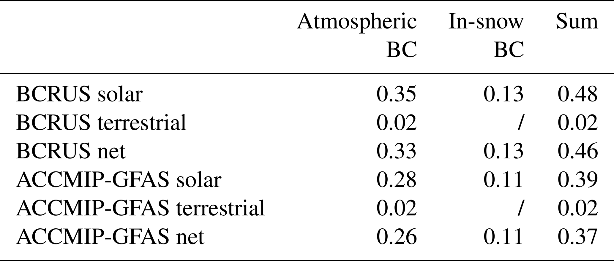
The BC-in-snow albedo effect for all-sky conditions is shown in Fig. 14b and f, as the 2005–2009 multi-year annual mean, for TOA and surface, respectively. The difference between TOA and surface is small and mainly caused by clouds. The effect is largest in coastal Greenland at around 1 W m−2, where snow is present throughout the year. Over the temporarily sea-ice- and snow-covered Arctic Ocean, the albedo effect varies by around 0.2 W m−2, which compensates the negative DRE of atmospheric BC at the BOA. On average the BC-in-snow albedo effect is 0.1 W m−2 in the Arctic (60–90∘ N; see Table 5). The sum of the DRE of BC in the atmosphere and snow is shown in Fig. 14c and g for the TOA and surface, respectively. Over the temporarily sea-ice-covered Arctic Ocean the BOA DRE of all BC (in the snow and atmosphere) is slightly positive (around 0.1 W m−2), while the TOA DRE is strongly positive, with values up to 1.9 W m−2. The resulting average for the Arctic region is 0.5 W m−2. Over the Arctic Ocean the DRE of atmospheric BC is in the range of the DRE considering all aerosol species (not shown) but smaller over the continents. The all-aerosol DRE at the TOA would therefore be negative if no BC were present in the Arctic atmosphere (−0.2 W m−2 in the spatial and annual average).
The difference between the model runs is used to estimate the emission-related uncertainty of the Arctic energy budget. Therefore, difference of the total radiative effect at TOA (all-sky conditions) of ACCMIP-GFAS minus BCRUS, as shown in Fig. 14h, is analyzed. In the ACCMIP-GFAS run, the TOA net all-sky positive radiative effect of BC is lower by 0.1 W m−2 in the regional average (60–90∘ N; see Table 5) but more than 0.2 W m−2 higher regionally over the Barents Sea and Kara Sea. At the surface the difference is smaller, with values of 0.05 W m−2 less in ACCMIP-GFAS over most of the Arctic, with the exception of parts of Russia, as shown in Fig. 14h. The more recent and transient emission data with local refinement therefore result in a considerably stronger climate forcing due to anthropogenic and biomass burning BC. This shows that the TOA DRE of BC is more sensitive to an increase in the BC burden due to the different emission setups than the BOA DRE, since the net energy gain caused by the reduction of the snow albedo is canceled out to some degree by the shadowing effect of atmospheric BC.

Figure 14Multi-year mean all-sky direct aerosol radiative effect (DRE) of BC for the period 2005–2009. Top row for top of the atmosphere (TOA) and bottom row for bottom of the atmosphere (BOA). (a) and (e) show the BCRUS net (terrestrial and solar) DRE of atmospheric BC, and (b) and (f) show solar BC-in-snow albedo radiative effect. (c) and (g) show the total of the radiative effects of BC in the atmosphere and deposited in snow (terrestrial plus solar). (d) and (e) show the difference in the total BC radiative effect between the runs ACCMIP-GFAS and BCRUS (ACCMIP-GFAS minus BCRUS).
We therefore conclude that, according to our best estimate, BC causes a net energy gain for the Arctic on the annual mean at TOA as well as BOA. The uncertainty with respect to the emission setup is roughly 25 % for TOA and BOA but stronger in absolute values at TOA. This is solely due to the uncertainties in emission; potential uncertainties in removal shown in the evaluation with observations are not included.
In this study, the representation of Arctic black carbon (BC) aerosol particles in the global aerosol-climate model ECHAM6.3-HAM2.3 is evaluated with respect to different emission inventories. As a reference BC measurements at Arctic sites and from aircraft campaigns are used comprehensively. By comparing the effects of different state-of-the-art BC emission inventories, an uncertainty range of current model estimates of the Arctic atmospheric BC burden and the local direct aerosol radiative effect (DRE) of BC is quantified. The uncertainties are explored with a focus on three influencing factors: (1) the influence of temporally variable biomass burning emissions, (2) the importance of recent air quality policies and economic developments, and (3) the potential improvements by regional refinements in Russian BC sources. This is achieved by comparing four different emission setups.
The run BCRUS represents a recent estimate of global emissions with the special feature of a high estimate in local Arctic emissions, especially in gas flaring. It uses anthropogenic emissions from the ECLIPSE emission data set, and in Russia the BC emissions of ECLIPSE are replaced with the higher-resolution and more recent data from Huang et al. (2015). For the biomass burning emissions, GFAS is used, which derives the location and amount of emitted gas and aerosol particles from satellite. The ECLIPSE run uses ECLIPSE emissions and GFAS emissions for the biomass burning emissions. For the ACCMIP run we use the anthropogenic part of the ACCMIP emissions, which are widely used. We fixed the emissions to year 2000, not taking into account the recent economic changes and variable biomass burning emissions. ACCMIP does not consider gas flaring emissions. In the run ACCMIP-GFAS, the fixed year 2000 biomass burning emissions are replaced by dynamic real-time fire data from GFAS. The emission factor of 3.4 that is commonly used for GFAS emissions (Kaiser et al., 2012) was not used, since it led to a strong overestimation in mid- and high-latitudinal BC concentrations in an early setup.
The comparison between ACCMIP and ACCMIP-GFAS is used to estimate the impact of temporally variable biomass burning emissions. ACCMIP-GFAS and BCRUS are used to quantify the impact of recent developments in air quality policies and economic developments. The difference between ECLIPSE and BCRUS shows the impact of a regional refinement.
The variable biomass burning emissions are not particularly important for the annual mean of the Arctic BC burden but are crucial for reproducing high-pollution events. The different assumptions on anthropogenic emission based on economic development and air quality policies result in an uncertainty in the BC burden of more than 50 µg m−2 over the Arctic Ocean, which is 20 % of the local annual mean BC load. The regional refinements in Russia mainly change the BC burden in this region and will improve the ability of the model to reproduce local measurements.
The near-surface BC concentrations could be reproduced to a reasonable accuracy by ECHAM-HAM in most cases. The exception from this are stations that are challenging because of their surrounding orography and the horizontal model resolution, namely Summit, Ny-Ålesund and Zeppelin Station, where ECHAM-HAM falsely produced similar peak concentrations in late winter and early spring as for all other stations. The sensitivity to the different emission setups is low in the summer. This is a result of low local emissions near the measurement sites in all runs and reduced long-range transport from the mid-latitudes as well as more precipitation in the summertime Arctic.
In the months with high modeled concentrations the model shows a high sensitivity to the changing emissions for the stations closest to the Arctic Ocean. The observed monthly median BC peak concentrations in Tiksi were underestimated by the model, but the run BCRUS that includes the most accurate gas flaring emissions produced the best results. For other stations, e.g., in Barrow in February, BCRUS showed a stronger overestimation than the other runs.
A similar pattern can be observed for Zeppelin Station, Ny-Ålesund, Villum Research Station and Alert. Higher emissions lead to higher concentrations, with no significant changes in the pattern of the annual cycle. Overall, however, it is difficult to decide which emission setup provides satisfactory agreement with the aerosol observations for all cases. This means that the annual cycle of Arctic stations reproduced by ECHAM-HAM is mainly controlled by the transport. Changing the amount and location by using a different emission setup only modulates the amount of the BC concentrations but unexpectedly does not affect the seasonality significantly.
The correlation coefficients of near-surface concentrations are generally reasonably good, at 0.45 and higher for most stations. This points toward a good agreement in the timing, especially of observed peak events. These peaks are most often caused by biomass burning. The exceptions are Summit, Simeonof, Zeppelin Station and Oulanka, with correlation coefficients below 0.3. The run ACCMIP is the only one that shows significantly smaller correlation coefficients, since the biomass burning emissions for this run are fixed and not prescribed on a daily basis from satellite observations.
The evaluation using a combination of aircraft campaigns shows that, in general, the vertical distribution is reproduced well by ECHAM-HAM. This improvement over older model versions is at least partly achieved with the aerosol size-dependent wet removal scheme by Croft et al. (2010). The model results look best during spring. In summer BC is systematically overestimated by the model at heights above 500 hPa. This overestimation has been described for several models in the AeroCom model intercomparison project before (Schwarz et al., 2013, 2017).
In one summer case of an observed wet removal affecting a biomass burning plume, described by Matsui et al. (2011), the model correctly reproduced the time and height of a biomass burning layer. It is known that reproducing individual pollution events in exactly the correct way is impossible for a global model with this resolution because both the aerosol transport and the wet removal are affected by subscale processes. ECHAM-HAM overestimated the BC concentrations because of this issue. While here the BC lifetime was overestimated, in general, the BC lifetime of ECHAM-HAM was considered to be reasonably good (Lund et al., 2018).
The ECHAM-HAM simulations show that over the Arctic Ocean the net (solar plus terrestrial) TOA DRE of atmospheric BC is positive, with an annual average of over 0.4 W m−2. The BC-in-snow albedo effect causes an additional energy gain for the Arctic system of around 0.2 W m−2 over the central Arctic. Locally larger effects are calculated for coastal Greenland. The BOA DRE is stronger than the shadowing effect of BC, causing a net energy gain. The emission-related uncertainty of DRE both at TOA and BOA is roughly 25 %.
Overall, the current model version of ECHAM6-HAM2 performs considerably better than in a previous model intercomparison study (Schwarz et al., 2017). In particular, the seasonality, but also the vertical distribution of BC aerosol in the Arctic, has improved. Reducing the overestimation of upper-level BC concentrations would be a big improvement, since this still causes large uncertainties in climate models and recent direct radiative forcing estimates. Here, especially the representation of wet scavenging and convective mixing needs to be improved, since it is the biggest BC sink in the Arctic.
The code for ECHAM-HAM is available to the scientific community according to the HAMMOZ Software License Agreement though the following project website: https://redmine.hammoz.ethz.ch/projects/hammoz (Hammoz, 2019). The model output data (Schacht et al., 2019) used for the plots are available through the World Data Center PANGAEA.
JS performed the ECHAM-HAM simulations, collected emission data and in situ measurement data from the providers, prepared the emissions, performed the analysis, and wrote the paper. BH provided support for the ECHAM-HAM simulations, suggested in situ measurement data providers, and provided advice during the analysis and on the project design. JQ, MZ, AE, JB and RC provided support in writing and designing the paper. RC gave advice on the emission data setup. WTKH provided the code and advice on the BC in snow parameterization for ECHAM-HAM. JB, AH, YK, AM, PRS, BW and MZ provided in situ measurement data and associated discussion. IT provided advice throughout the project design, setup, analysis and writing progress.
The authors declare that they have no conflict of interest.
We gratefully acknowledge the funding by the Deutsche Forschungsgemeinschaft (DFG; German Research Foundation; project number 268020496; TRR 172) within the Transregional Collaborative Research Centre “ArctiC Amplification: Climate Relevant Atmospheric and SurfaCe Processes, and Feedback Mechanisms (AC)3”. Ribu Cherian was supported by the DFG project under grant agreement no. 637230. Bernadett Weinzierl received funding from the European Research Council under the European Community's Horizon 2020 research and innovation framework program under grant agreement no. 640458 (A-LIFE). The DLR SP2 data were obtained with the support of the European Union under grant agreement no. 265863 (ACCESS) and the Helmholtz Association under grant agreement VH-NG-606 (Helmholtz-Hochschul-Nachwuchsgruppe AerCARE). The Arctic data used in this article and managed by ACTRIS are archived and accessible from the EBAS database operated at the Norwegian Institute for Air Research (NILU; http://ebas.nilu.no, last access: 17 December 2018). ACTRIS data management is provided by the WMO Global Atmosphere Watch World Data Centre for Aerosols. The ACTRIS project, providing the data, has received funding from the European Union's Horizon 2020 research and innovation program under grant agreement no. 654109 (ACTRIS). We thank the providers of the Arctic data. ALERT data are from Environment and Climate Change Canada, Sangeeta Sharma, all technicians and operators, and the Canadian Department of National Defence. BARROW data are from Patrick Sheridan, Elisabeth Andrews and Betsy Andrews (NOAA Oceanic and Atmospheric Research/GMD). SUMMIT data are from Patrick Sheridan, Elisabeth Andrews and Betsy Andrews (NOAA Oceanic and Atmospheric Research/GMD); Michael Bergin (Duke University); and the National Science Foundation (OPP 1546002). TIKSI data are from Sara Morris (NOAA Oceanic and Atmospheric Research/GMD) and the Academy of Finland project Greenhouse gas, aerosol and albedo variations in the changing Arctic (project number 269095). PALLAS data are from the Academy of Finland project Greenhouse gas, aerosol and albedo variations in the changing Arctic (project number 269095); the Academy of Finland project Novel Assessment of Black Carbon in the Eurasian Arctic: From Historical Concentrations and Sources to Future Climate Impacts (NABCEA), project number 296302; and the Academy of Finland Centre of Excellence Programme (project number 307331). ZEPPELIN data are from the Swedish Environmental Protection Agency (Naturvårdsverket), Vetenskaprådet, FORMAS, the NILU (Norsk institutt for luftforskning) and Peter Tunved (Stockholm University). The research leading to these results has received funding from the European Union's Horizon 2020 research and innovation program under grant agreement no. 654109. IMPROVE is a collaborative association of state, tribal and federal agencies and international partners. The US Environmental Protection Agency is the primary funding source, with contracting and research support from the National Park Service. The Air Quality Group at the University of California, Davis, is the central analytical laboratory, with ion analysis provided by Research Triangle Institute and carbon analysis provided by the Desert Research Institute. We thank the principal investigators Brent Holben, Ihab Abboud, Antti Arola, Vitali Fioletov, Laurie Gregory, Rigel Kivi, Lynn Ma, Norm O’Neill, Mikhail Panchenko, Piotr Sobolewski, John R. Vande Castle and Rick Wagener; the co-investigators Piotr Glowacki, Grzegorz Karasiski and Sergey Sakerin; and their staff for establishing and maintaining the AERONET sites used in this investigation. The HIPPO 1–5 data were provided by NCAR/EOL under the sponsorship of the National Science Foundation (https://data.eol.ncar.edu/, last access: 12 June 2018). We would also like to thank the German Climate Computing Center (Deutsches Klimarechenzentrum; DKRZ) for the computing time and their services. We especially thank the developers of ECHAM-HAM. The ECHAM-HAMMOZ model is developed by a consortium composed of ETH Zürich, Max Planck Institute for Meteorology, Forschungszentrum Jülich, the University of Oxford, the Finnish Meteorological Institute and the Leibniz Institute for Tropospheric Research and managed by the Center for Climate Systems Modeling (C2SM) at ETH Zürich. Finally, we would like to thank the anonymous reviewers of this article for their constructive and valuable comments.
This paper was edited by Kari Lehtinen and reviewed by three anonymous referees.
Arnold, S., Law, K., Brock, C., Thomas, J., Starkweather, S., Salzen, K. V., Stohl, A., Sharma, S., Lund, M., Flanner, M., Petäjä, T., Tanimoto, H., Gamble, J., Dibb, J., Melamed, M., Johnson, N., Fidel, M., Tynkkynen, V.-P., Baklanov, A., Eckhardt, S., Monks, S., Browse, J., and Bozem, H.: Arctic air pollution: Challenges and opportunities for the next decade, ELEMENTA – Science of the Antropocene, 4, 000104, https://doi.org/10.12952/journal.elementa.000104, 2016. a
Backman, J., Schmeisser, L., Virkkula, A., Ogren, J. A., Asmi, E., Starkweather, S., Sharma, S., Eleftheriadis, K., Uttal, T., Jefferson, A., Bergin, M., Makshtas, A., Tunved, P., and Fiebig, M.: On Aethalometer measurement uncertainties and an instrument correction factor for the Arctic, Atmos. Meas. Tech., 10, 5039–5062, https://doi.org/10.5194/amt-10-5039-2017, 2017a. a
Backman, J., Schmeisser, L., Virkkula, A., Ogren, J. A., Asmi, E., Starkweather, S., Sharma, S., Eleftheriadis, K., Vratolis, S., Uttal, T., Tunved, P., Jefferson, A., Bergin, M., Makshtas, A., and Fiebig, M.: Time series of aerosol light-absorption coefficients from Aethalometers at six Arctic stations between 2012 and 2014, data retrieved from World Development Indicators, https://doi.org/10.21336/gen.1, 2017b. a, b
Bond, T. C., Streets, D. G., Yarber, K. F., Nelson, S. M., Woo, J.-H., and Klimont, Z.: A technology-based global inventory of black and organic carbon emissions from combustion, J. Geophys. Res.-Atmos., 109, D14, https://doi.org/10.1029/2003JD003697, 2004. a
Bond, T. C., Doherty, S. J., Fahey, D. W., Forster, P. M., Berntsen, T., DeAngelo, B. J., Flanner, M. G., Ghan, S., Kärcher, B., Koch, D., Kinne, S., Kondo, Y., Quinn, P. K., Sarofim, M. C., Schultz, M. G., Schulz, M., Venkataraman, C., Zhang, H., Zhang, S., Bellouin, N., Guttikunda, S. K., Hopke, P. K., Jacobson, M. Z., Kaiser, J. W., Klimont, Z., Lohmann, U., Schwarz, J. P., Shindell, D., Storelvmo, T., Warren, S. G., and Zender, C. S.: Bounding the role of black carbon in the climate system: A scientific assessment, J. Geophys. Res.-Atmos., 118, 5380–5552, https://doi.org/10.1002/jgrd.50171, 2013. a
Chow, J. C., Watson, J. G., Chen, L.-W. A., Chang, M. O., Robinson, N. F., Trimble, D., and Kohl, S.: The IMPROVE_A Temperature Protocol for Thermal/Optical Carbon Analysis: Maintaining Consistency with a Long-Term Database, J. Air Waste Manage., 57, 1014–1023, https://doi.org/10.3155/1047-3289.57.9.1014, 2007. a
Corbett, J. J., Lack, D. A., Winebrake, J. J., Harder, S., Silberman, J. A., and Gold, M.: Arctic shipping emissions inventories and future scenarios, Atmos. Chem. Phys., 10, 9689–9704, https://doi.org/10.5194/acp-10-9689-2010, 2010. a
Croft, B., Lohmann, U., Martin, R. V., Stier, P., Wurzler, S., Feichter, J., Hoose, C., Heikkilä, U., van Donkelaar, A., and Ferrachat, S.: Influences of in-cloud aerosol scavenging parameterizations on aerosol concentrations and wet deposition in ECHAM5-HAM, Atmos. Chem. Phys., 10, 1511–1543, https://doi.org/10.5194/acp-10-1511-2010, 2010. a
Eckhardt, S., Quennehen, B., Olivié, D. J. L., Berntsen, T. K., Cherian, R., Christensen, J. H., Collins, W., Crepinsek, S., Daskalakis, N., Flanner, M., Herber, A., Heyes, C., Hodnebrog, Ø., Huang, L., Kanakidou, M., Klimont, Z., Langner, J., Law, K. S., Lund, M. T., Mahmood, R., Massling, A., Myriokefalitakis, S., Nielsen, I. E., Nøjgaard, J. K., Quaas, J., Quinn, P. K., Raut, J.-C., Rumbold, S. T., Schulz, M., Sharma, S., Skeie, R. B., Skov, H., Uttal, T., von Salzen, K., and Stohl, A.: Current model capabilities for simulating black carbon and sulfate concentrations in the Arctic atmosphere: a multi-model evaluation using a comprehensive measurement data set, Atmos. Chem. Phys., 15, 9413–9433, https://doi.org/10.5194/acp-15-9413-2015, 2015. a, b, c
Eckhardt, S., Cassiani, M., Evangeliou, N., Sollum, E., Pisso, I., and Stohl, A.: Source-receptor matrix calculation for deposited mass with the Lagrangian particle dispersion model FLEXPART v10.2 in backward mode, Geosci. Model Dev., 10, 4605–4618, https://doi.org/10.5194/gmd-10-4605-2017, 2017. a
Flanner, M. G., Zender, C. S., Randerson, J. T., and Rasch, P. J.: Present-day climate forcing and response from black carbon in snow, J. Geophys. Res.-Atmos., 112, D11202, https://doi.org/10.1029/2006JD008003, 2007. a, b
Gilgen, A., Huang, W. T. K., Ickes, L., Neubauer, D., and Lohmann, U.: How important are future marine and shipping aerosol emissions in a warming Arctic summer and autumn?, Atmos. Chem. Phys., 18, 10521–10555, https://doi.org/10.5194/acp-18-10521-2018, 2018. a, b, c
Hammoz: ECHAM-HAMMOZ, available at: https://redmine.hammoz.ethz.ch/projects/hammoz, last access: 9 May 2019. a
Herber, A. B., Haas, C., Stone, R. S., Bottenheim, J. W., Liu, P., Li, S.-M., Staebler, R. M., Strapp, J. W., and Dethloff, K.: Regular airborne surveys of Arctic sea ice and atmosphere, Eos, Transactions American Geophysical Union, 93, 41–42, https://doi.org/10.1029/2012EO040001, 2012. a, b
Huang, K., Fu, J. S., Prikhodko, V. Y., Storey, J. M., Romanov, A., Hodson, E. L., Cresko, J., Morozova, I., Ignatieva, Y., and Cabaniss, J.: Russian anthropogenic black carbon: Emission reconstruction and Arctic black carbon simulation, J. Geophys. Res.-Atmos., 120, 11306–11333, https://doi.org/10.1002/2015JD023358, 2015. a, b, c, d, e, f
Ikeda, K., Tanimoto, H., Sugita, T., Akiyoshi, H., Kanaya, Y., Zhu, C., and Taketani, F.: Tagged tracer simulations of black carbon in the Arctic: transport, source contributions, and budget, Atmos. Chem. Phys., 17, 10515–10533, https://doi.org/10.5194/acp-17-10515-2017, 2017. a
Jacob, D. J., Crawford, J. H., Maring, H., Clarke, A. D., Dibb, J. E., Emmons, L. K., Ferrare, R. A., Hostetler, C. A., Russell, P. B., Singh, H. B., Thompson, A. M., Shaw, G. E., McCauley, E., Pederson, J. R., and Fisher, J. A.: The Arctic Research of the Composition of the Troposphere from Aircraft and Satellites (ARCTAS) mission: design, execution, and first results, Atmos. Chem. Phys., 10, 5191–5212, https://doi.org/10.5194/acp-10-5191-2010, 2010. a, b
Kaiser, J. W., Heil, A., Andreae, M. O., Benedetti, A., Chubarova, N., Jones, L., Morcrette, J.-J., Razinger, M., Schultz, M. G., Suttie, M., and van der Werf, G. R.: Biomass burning emissions estimated with a global fire assimilation system based on observed fire radiative power, Biogeosciences, 9, 527–554, https://doi.org/10.5194/bg-9-527-2012, 2012. a, b, c
Klimont, Z., Kupiainen, K., Heyes, C., Purohit, P., Cofala, J., Rafaj, P., Borken-Kleefeld, J., and Schöpp, W.: Global anthropogenic emissions of particulate matter including black carbon, Atmos. Chem. Phys., 17, 8681–8723, https://doi.org/10.5194/acp-17-8681-2017, 2017. a
Koch, D., Schulz, M., Kinne, S., McNaughton, C., Spackman, J. R., Balkanski, Y., Bauer, S., Berntsen, T., Bond, T. C., Boucher, O., Chin, M., Clarke, A., De Luca, N., Dentener, F., Diehl, T., Dubovik, O., Easter, R., Fahey, D. W., Feichter, J., Fillmore, D., Freitag, S., Ghan, S., Ginoux, P., Gong, S., Horowitz, L., Iversen, T., Kirkevåg, A., Klimont, Z., Kondo, Y., Krol, M., Liu, X., Miller, R., Montanaro, V., Moteki, N., Myhre, G., Penner, J. E., Perlwitz, J., Pitari, G., Reddy, S., Sahu, L., Sakamoto, H., Schuster, G., Schwarz, J. P., Seland, Ø., Stier, P., Takegawa, N., Takemura, T., Textor, C., van Aardenne, J. A., and Zhao, Y.: Evaluation of black carbon estimations in global aerosol models, Atmos. Chem. Phys., 9, 9001–9026, https://doi.org/10.5194/acp-9-9001-2009, 2009. a
Kodros, J. K., Hanna, S. J., Bertram, A. K., Leaitch, W. R., Schulz, H., Herber, A. B., Zanatta, M., Burkart, J., Willis, M. D., Abbatt, J. P. D., and Pierce, J. R.: Size-resolved mixing state of black carbon in the Canadian high Arctic and implications for simulated direct radiative effect, Atmos. Chem. Phys., 18, 11345–11361, https://doi.org/10.5194/acp-18-11345-2018, 2018. a
Lamarque, J.-F., Bond, T. C., Eyring, V., Granier, C., Heil, A., Klimont, Z., Lee, D., Liousse, C., Mieville, A., Owen, B., Schultz, M. G., Shindell, D., Smith, S. J., Stehfest, E., Van Aardenne, J., Cooper, O. R., Kainuma, M., Mahowald, N., McConnell, J. R., Naik, V., Riahi, K., and van Vuuren, D. P.: Historical (1850–2000) gridded anthropogenic and biomass burning emissions of reactive gases and aerosols: methodology and application, Atmos. Chem. Phys., 10, 7017–7039, https://doi.org/10.5194/acp-10-7017-2010, 2010. a
Law, K. S. and Stohl, A.: Arctic Air Pollution: Origins and Impacts, Science, 315, 1537–1540, https://doi.org/10.1126/science.1137695, 2007. a, b
Lohmann, U., Spichtinger, P., Jess, S., Peter, T., and Smit, H. G. J.: Cirrus cloud formation and ice supersaturated regions in a global climate model, Environ. Res. Lett., 3, 1748–9326, https://doi.org/10.1088/1748-9326/3/4/045022, 2008. a
Lund, M. T., Samset, B. r. H., Skeie, R. B., Watson-Parris, D., Katich, J. M., Schwarz, J. P., and Weinzierl, B.: Short Black Carbon lifetime inferred from a global set of aircraft observations, npj Climate and Atmospheric Science, 1, 2397–3722 https://doi.org/10.1038/s41612-018-0040-x, 2018. a, b, c
Massling, A., Nielsen, I. E., Kristensen, D., Christensen, J. H., Sørensen, L. L., Jensen, B., Nguyen, Q. T., Nøjgaard, J. K., Glasius, M., and Skov, H.: Atmospheric black carbon and sulfate concentrations in Northeast Greenland, Atmos. Chem. Phys., 15, 9681–9692, https://doi.org/10.5194/acp-15-9681-2015, 2015. a, b
Matsui, H., Kondo, Y., Moteki, N., Takegawa, N., Sahu, L. K., Koike, M., Zhao, Y., Fuelberg, H. E., Sessions, W. R., Diskin, G., Anderson, B. E., Blake, D. R., Wisthaler, A., Cubison, M. J., and Jimenez, J. L.: Accumulation-mode aerosol number concentrations in the Arctic during the ARCTAS aircraft campaign: Long-range transport of polluted and clean air from the Asian continent, J. Geophys. Res.-Atmos., 116, D20, https://doi.org/10.1029/2011JD016189, 2011. a, b, c, d
Petoukhov, V. and Semenov, V. A.: A link between reduced Barents-Kara sea ice and cold winter extremes over northern continents, J. Geophys. Res.-Atmos., 115, D21111, https://doi.org/10.1029/2009JD013568, 2010. a
Quinn, P., AMAP, and Stohl, A.: AMAP Assessment 2015: Black Carbon and Ozone as Arctic Climate Forcers, Arctic Monitoring and Assessment Programme (AMAP), Oslo, Norway, available at: https://www.amap.no/documents/download/2506 (last access: 5 May 2017), 2015. a
Roiger, A., Thomas, J.-L., Schlager, H., Law, K. S., Kim, J., Schäfler, A., Weinzierl, B., Dahlkötter, F., Krisch, I., Marelle, L., Minikin, A., Raut, J.-C., Reiter, A., Rose, M., Scheibe, M., Stock, P., Baumann, R., Bouarar, I., Clerbaux, C., George, M., Onishi, T., and Flemming, J.: Quantifying Emerging Local Anthropogenic Emissions in the Arctic Region: The ACCESS Aircraft Campaign Experiment, B. Am. Meteorol. Soc., 96, 441–460, https://doi.org/10.1175/BAMS-D-13-00169.1, 2015. a, b
Samset, B. H., Myhre, G., Schulz, M., Balkanski, Y., Bauer, S., Berntsen, T. K., Bian, H., Bellouin, N., Diehl, T., Easter, R. C., Ghan, S. J., Iversen, T., Kinne, S., Kirkevåg, A., Lamarque, J.-F., Lin, G., Liu, X., Penner, J. E., Seland, Ø., Skeie, R. B., Stier, P., Takemura, T., Tsigaridis, K., and Zhang, K.: Black carbon vertical profiles strongly affect its radiative forcing uncertainty, Atmos. Chem. Phys., 13, 2423–2434, https://doi.org/10.5194/acp-13-2423-2013, 2013. a
Sand, M., Berntsen, T. K., Kay, J. E., Lamarque, J. F., Seland, Ø., and Kirkevåg, A.: The Arctic response to remote and local forcing of black carbon, Atmos. Chem. Phys., 13, 211–224, https://doi.org/10.5194/acp-13-211-2013, 2013. a
Sand, M., Berntsen, T., von Salzen, K., Flanner, M., Langner, J., and G. Victor, D.: Response of Arctic temperature to changes in emissions of short-lived climate forcers, 6, 286–289, https://doi.org/10.1038/nclimate2880, 2015. a
Sand, M., Samset, B. H., Balkanski, Y., Bauer, S., Bellouin, N., Berntsen, T. K., Bian, H., Chin, M., Diehl, T., Easter, R., Ghan, S. J., Iversen, T., Kirkevåg, A., Lamarque, J.-F., Lin, G., Liu, X., Luo, G., Myhre, G., Noije, T. V., Penner, J. E., Schulz, M., Seland, Ø., Skeie, R. B., Stier, P., Takemura, T., Tsigaridis, K., Yu, F., Zhang, K., and Zhang, H.: Aerosols at the poles: an AeroCom Phase II multi-model evaluation, Atmos. Chem. Phys., 17, 12197–12218, https://doi.org/10.5194/acp-17-12197-2017, 2017. a, b
Schacht, J., Heinold, B., and Tegen, I.: ECHAM-HAM simulations for evaluation and quantification of BC effects in the Arctic under different emission data sets, Leibniz-Institut für Troposphärenforschung e.V., Leipzig, PANGAEA, available at: https://doi.org/10.1594/PANGAEA.903547, last access: 6 July 2019. a
Schutgens, N. A. J., Gryspeerdt, E., Weigum, N., Tsyro, S., Goto, D., Schulz, M., and Stier, P.: Will a perfect model agree with perfect observations? The impact of spatial sampling, Atmos. Chem. Phys., 16, 6335–6353, https://doi.org/10.5194/acp-16-6335-2016, 2016. a
Schwarz, J. P., Samset, B. H., Perring, A. E., Spackman, J. R., Gao, R. S., Stier, P., Schulz, M., Moore, F. L., Ray, E. A., and Fahey, D. W.: Global-scale seasonally resolved black carbon vertical profiles over the Pacific, Geophys. Res. Lett., 40, 5542–5547, https://doi.org/10.1002/2013GL057775, 2013. a, b, c
Schwarz, J. P., Weinzierl, B., Samset, B. r. H., Dollner, M., Heimerl, K., Markovic, M. Z., Perring, A. E., and Ziemba, L.: Aircraft measurements of black carbon vertical profiles show upper tropospheric variability and stability, Geophys. Res. Lett., 44, 1132–1140, https://doi.org/10.1002/2016GL071241, 2017. a, b
Shaw, G. E.: The Arctic Haze Phenomenon, B. Am. Meteorol. Soc., 76, 2403–2414, https://doi.org/10.1175/1520-0477(1995)076<2403:TAHP>2.0.CO;2, 1995. a
Shindell, D.: Local and remote contributions to Arctic warming, Geophys. Res. Lett., 34, L14704, https://doi.org/10.1029/2007GL030221, 2007. a
Shindell, D. T., Chin, M., Dentener, F., Doherty, R. M., Faluvegi, G., Fiore, A. M., Hess, P., Koch, D. M., MacKenzie, I. A., Sanderson, M. G., Schultz, M. G., Schulz, M., Stevenson, D. S., Teich, H., Textor, C., Wild, O., Bergmann, D. J., Bey, I., Bian, H., Cuvelier, C., Duncan, B. N., Folberth, G., Horowitz, L. W., Jonson, J., Kaminski, J. W., Marmer, E., Park, R., Pringle, K. J., Schroeder, S., Szopa, S., Takemura, T., Zeng, G., Keating, T. J., and Zuber, A.: A multi-model assessment of pollution transport to the Arctic, Atmos. Chem. Phys., 8, 5353–5372, https://doi.org/10.5194/acp-8-5353-2008, 2008. a
Shindell, D. T., Faluvegi, G., Koch, D. M., Schmidt, G. A., Unger, N., and Bauer, S. E.: Improved Attribution of Climate Forcing to Emissions, Science, 326, 716–718, https://doi.org/10.1126/science.1174760, 2009. a
Sinha, P. R., Kondo, Y., Koike, M., Ogren, J. A., Jefferson, A., Barrett, T. E., Sheesley, R. J., Ohata, S., Moteki, N., Coe, H., Liu, D., Irwin, M., Tunved, P., Quinn, P. K., and Zhao, Y.: Evaluation of ground-based black carbon measurements by filter-based photometers at two Arctic sites, J. Geophys. Res.-Atmos., 122, 3544–3572, https://doi.org/10.1002/2016JD025843, 2017. a, b
Sofiev, M., Vankevich, R., Lotjonen, M., Prank, M., Petukhov, V., Ermakova, T., Koskinen, J., and Kukkonen, J.: An operational system for the assimilation of the satellite information on wild-land fires for the needs of air quality modelling and forecasting, Atmos. Chem. Phys., 9, 6833–6847, https://doi.org/10.5194/acp-9-6833-2009, 2009. a
Stevens, B., Giorgetta, M., Esch, M., Mauritsen, T., Crueger, T., Rast, S., Salzmann, M., Schmidt, H., Bader, J., Block, K., Brokopf, R., Fast, I., Kinne, S., Kornblueh, L., Lohmann, U., Pincus, R., Reichler, T., and Roeckner, E.: Atmospheric component of the MPI-M Earth System Model: ECHAM6, J. Adv. Model. Earth Sy., 5, 146–172, https://doi.org/10.1002/jame.20015, 2013. a
Stier, P., Feichter, J., Kinne, S., Kloster, S., Vignati, E., Wilson, J., Ganzeveld, L., Tegen, I., Werner, M., Balkanski, Y., Schulz, M., Boucher, O., Minikin, A., and Petzold, A.: The aerosol-climate model ECHAM5-HAM, Atmos. Chem. Phys., 5, 1125–1156, https://doi.org/10.5194/acp-5-1125-2005, 2005. a, b, c
Stohl, A., Klimont, Z., Eckhardt, S., Kupiainen, K., Shevchenko, V. P., Kopeikin, V. M., and Novigatsky, A. N.: Black carbon in the Arctic: the underestimated role of gas flaring and residential combustion emissions, Atmos. Chem. Phys., 13, 8833–8855, https://doi.org/10.5194/acp-13-8833-2013, 2013. a, b, c, d, e, f, g
Tegen, I. and Heinold, B.: Large-Scale Modeling of Absorbing Aerosols and Their Semi-Direct Effects, Atmosphere, 9, 10, https://doi.org/10.3390/atmos9100380, 2018. a
Tegen, I., Neubauer, D., Ferrachat, S., Siegenthaler-Le Drian, C., Bey, I., Schutgens, N., Stier, P., Watson-Parris, D., Stanelle, T., Schmidt, H., Rast, S., Kokkola, H., Schultz, M., Schroeder, S., Daskalakis, N., Barthel, S., Heinold, B., and Lohmann, U.: The global aerosol–climate model ECHAM6.3–HAM2.3 – Part 1: Aerosol evaluation, Geosci. Model Dev., 12, 1643–1677, https://doi.org/10.5194/gmd-12-1643-2019, 2019. a, b
Trenberth, K. E., Jones, P. D., Ambenje, P., Bojariu, R., Easterling, D., Klein Tank, A., Parker, D., Rahimzadeh, F., Renwick, J. A., Rusticucci, M., Soden, B., and Zhai, P.: Observations: Surface and Atmospheric Climate Change, in: Climate Change 2007: The Physical Science Basis, Contribution of Working Group I to the Fourth Assessment Report of the Intergovernmental Panel on Climate Change, edited by: Solomon, S., Qin, D., Manning, M., Chen, Z., Marquis, M., Averyt, K. B., Tignor, M., and Miller, H. L., Cambridge University Press, Cambridge, United Kingdom and New York, NY, USA, 2007. a
van Vuuren, D. P., Edmonds, J., Kainuma, M., Riahi, K., Thomson, A., Hibbard, K., Hurtt, G. C., Kram, T., Krey, V., Lamarque, J.-F., Masui, T., Meinshausen, M., Nakicenovic, N., Smith, S. J., and Rose, S. K.: The representative concentration pathways: an overview, Clim. Change, 109, 5, https://doi.org/10.1007/s10584-011-0148-z, 2011. a
Vignati, E., Wilson, J., and Stier, P.: M7: An efficient size-resolved aerosol microphysics module for large-scale aerosol transport models, J. Geophys. Res.-Atmos., 109, D22, https://doi.org/10.1029/2003JD004485, 2004. a
Vignati, E., Karl, M., Krol, M., Wilson, J., Stier, P., and Cavalli, F.: Sources of uncertainties in modelling black carbon at the global scale, Atmos. Chem. Phys., 10, 2595–2611, https://doi.org/10.5194/acp-10-2595-2010, 2010. a, b
Wendisch, M., Brückner, M., Burrows, J. P., Crewell, S., Dethloff, K., Ebell, K., Lüpkes, C., Macke, A., Notholt, J., Quaas, J., Rinke, A., and Tegen, I.: Understanding causes and effects of rapid warming in the Arctic, Eos, 98, 22–26, https://doi.org/10.1029/2017EO064803, 2017. a
Wendisch, M., Macke, A., Ehrlich, A., Lüpkes, C., Mech, M., Chechin, D., Dethloff, K., Barientos, C., Bozem, H., Brückner, M., Clemen, H.-C., Crewell, S., Donth, T., Dupuy, R., Ebell, K., Egerer, U., Engelmann, R., Engler, C., Eppers, O., Gehrmann, M., Gong, X., Gottschalk, M., Gourbeyre, C., Griesche, H., Hartmann, J., Hartmann, M., Heinold, B., Herber, A., Herrmann, H., Heygster, G., Hoor, P., Jafariserajehlou, S., Jäkel, E., Järvinen, E., Jourdan, O., Kästner, U., Kecorius, S., Knudsen, E. M., Köllner, F., Kretzschmar, J., Lelli, L., Leroy, D., Maturilli, M., Mei, L., Mertes, S., Mioche, G., Neuber, R., Nicolaus, M., Nomokonova, T., Notholt, J., Palm, M., van Pinxteren, M., Quaas, J., Richter, P., Ruiz-Donoso, E., Schäfer, M., Schmieder, K., Schnaiter, M., Schneider, J., Schwarzenböck, A., Seifert, P., Shupe, M. D., Siebert, H., Spreen, G., Stapf, J., Stratmann, F., Vogl, T., Welti, A., Wex, H., Wiedensohler, A., Zanatta, M., and Zeppenfeld, S.: The Arctic Cloud Puzzle: Using ACLOUD/PASCAL Multi-Platform Observations to Unravel the Role of Clouds and Aerosol Particles in Arctic Amplification, B. Am. Meteorol. Soc., 100, 841–871, https://doi.org/10.1175/BAMS-D-18-0072.1, 2018. a, b
Winiger, P., Andersson, A., Eckhardt, S., Stohl, A., Semiletov, I. P., Dudarev, O. V., Charkin, A., Shakhova, N., Klimont, Z., Heyes, C., and Gustafsson, Ö.: Siberian Arctic black carbon sources constrained by model and observation, P. Natl. Acad. Sci. USA, 7, 1054–1061, https://doi.org/10.1073/pnas.1613401114, 2017. a, b
Wofsy, S. C., Daube, B., Jimenez, R., Kort, E., Pittman, J. V., Park, S., Commane, R., Xian g, B., Santoni, G., Jacob, D. J., Fisher, J. A., Heaps, C. A. Pickett-and Wang, H., Wecht, K. J., Wang, Q., Stephens, B. B., Shertz, S., Watt, A., Romashkin, P., Campos, T., Haggerty, J., Coo per, W. A., Rogers, D. C., Beaton, S., Hendershot, R., Elkins, J. W., Fahey, D. W., Gao, R.-S., Schwarz, J. P., Moore, F., Montzka, S. A., Perring, A. E., Hurst, D., Miller, B. R., Sweeney, C., Oltmans, S. J., Hintsa, E., Nance, D., Dutton, G. S., Watts, L. A., Spackman, J. R., Rosenlof, K. H., Ray, E., Hall, B., Zondlo, M., Diao, M., Keeling, R. F., Bent, J., Atlas, E., Lueb, R., and Mahoney, M. J.: HIPPO Merged 10-Second Meteorology, Atmospheric Chemistry, and Aerosol Dat, Version 1.0., dat retrieved from UCAR/NCAR – Earth Observing Laboratory, available at: https://doi.org/10.3334/CDIAC/HIPPO_010 (last access: 12 June 2018), 2017. a, b
Zanatta, M., Gysel, M., Bukowiecki, N., Müller, T., Weingartner, E., Areskoug, H., Fiebig, M., Yttri, K., Mihalopoulos, N., Kouvarakis, G., Beddows, D., Harrison, R., Cavalli, F., Putaud, J., Spindler, G., Wiedensohler, A., Alastuey, A., Pandolfi, M., Sellegri, K., Swietlicki, E., Jaffrezo, J., Baltensperger, U., and Laj, P.: A European aerosol phenomenology-5: Climatology of black carbon optical properties at 9 regional background sites across Europe, Atmos. Environ., 145, 346–364, https://doi.org/10.1016/j.atmosenv.2016.09.035, 2016. a
Zanatta, M., Laj, P., Gysel, M., Baltensperger, U., Vratolis, S., Eleftheriadis, K., Kondo, Y., Dubuisson, P., Winiarek, V., Kazadzis, S., Tunved, P., and Jacobi, H.-W.: Effects of mixing state on optical and radiative properties of black carbon in the European Arctic, Atmos. Chem. Phys., 18, 14037–14057, https://doi.org/10.5194/acp-18-14037-2018, 2018. a, b
Zhang, K., O'Donnell, D., Kazil, J., Stier, P., Kinne, S., Lohmann, U., Ferrachat, S., Croft, B., Quaas, J., Wan, H., Rast, S., and Feichter, J.: The global aerosol-climate model ECHAM-HAM, version 2: sensitivity to improvements in process representations, Atmos. Chem. Phys., 12, 8911–8949, https://doi.org/10.5194/acp-12-8911-2012, 2012. a, b, c, d, e, f, g