Core and margin in warm convective clouds – Part 1: Core types and evolution during a cloud's lifetime

Heiblum, Reuven H.; Pinto, Lital; Altaratz, Orit; Dagan, Guy; Koren, Ilan

doi:https://doi.org/10.5194/acp-19-10717-2019

Articles | Volume 19, issue 16

https://doi.org/10.5194/acp-19-10717-2019

Articles | Volume 19, issue 16

Research article

26 Aug 2019

Research article |

| 26 Aug 2019

Core and margin in warm convective clouds – Part 1: Core types and evolution during a cloud's lifetime

Reuven H. Heiblum, Lital Pinto, Orit Altaratz, Guy Dagan, and Ilan Koren

Abstract

The properties of a warm convective cloud are determined by the competition between the growth and dissipation processes occurring within it. One way to observe and follow this competition is by partitioning the cloud to core and margin regions. Here we look at three core definitions, namely positive vertical velocity (W_core), supersaturation (RH_core), and positive buoyancy (B_core), and follow their evolution throughout the lifetime of warm convective clouds.

Using single cloud and cloud field simulations with bin-microphysics schemes, we show that the different core types tend to be subsets of one another in the following order: $B_{core} \subseteq {RH}_{core} \subseteq W_{core}$ . This property is seen for several different thermodynamic profile initializations and is generally maintained during the growing and mature stages of a cloud's lifetime. This finding is in line with previous works and theoretical predictions showing that cumulus clouds may be dominated by negative buoyancy at certain stages of their lifetime. The RH_core–W_core pair is most interchangeable, especially during the growing stages of the cloud.

For all three definitions, the core–shell model of a core (positive values) at the center of the cloud surrounded by a shell (negative values) at the cloud periphery applies to over 80 % of a typical cloud's lifetime. The core–shell model is less appropriate in larger clouds with multiple cores displaced from the cloud center. Larger clouds may also exhibit buoyancy cores centered near the cloud edge. During dissipation the cores show less overlap, reduce in size, and may migrate from the cloud center.

Download & links

How to cite

How to cite.

Dates

Received: 29 Jul 2018 – Discussion started: 30 Aug 2018 – Revised: 28 Apr 2019 – Accepted: 05 Jun 2019 – Published: 26 Aug 2019

1 Introduction

Clouds are important players in the climate system (Trenberth et al., 2009) and currently constitute one of the largest uncertainties in climate and climate change research (IPCC, 2013). One of the reasons for this large uncertainty is the complexity created by opposing processes that occur at the same time but in different locations within a cloud. Although a cloud is generally considered to be a single entity, physically, it can be partitioned to two main regions: (i) a core region, where mainly cloud growth processes occur (i.e., condensation – accumulation of cloud mass), and (ii) a margin region, where cloud suppression processes occur (i.e., evaporation – loss of cloud mass). Changes in thermodynamic or microphysical (aerosol) conditions impact the processes in both regions (sometimes in different ways) and thus the resultant total cloud properties (Dagan et al., 2015). To better understand cloud properties and their evolution in time, it is necessary to understand the interplay between physical processes within the core and margin regions (and the way they are affected by perturbations in the environmental conditions).

Considering convective clouds, there are several objective measures that have been used in previous works for separating a cloud's core from its margins (this will be referred to as physical cores hereafter). In deep convective cloud simulations the core is usually defined by the updrafts' magnitude using a certain threshold, usually W>1 m s⁻¹ (Khairoutdinov et al., 2009; Kumar et al., 2015; Lebo and Seinfeld, 2011; Morrison, 2012). Studies on warm cumulus clouds have defined the clouds' core as parts with positive buoyancy and positive updrafts (Dawe and Austin, 2012; de Roode et al., 2012; Heus and Jonker, 2008; Siebesma and Cuijpers, 1995) or solely regions with positively buoyancy (Heus and Seifert, 2013; Seigel, 2014). More recently, cloud partition to regions of supersaturation, and sub-saturation has been used to define the cloud core in single cloud simulations (Dagan et al., 2015).

For simplicity, we focus on warm convective clouds (only contain liquid water), avoiding the additional complexity and uncertainties associated with mixed-phase and ice-phase microphysics. The common assumption when partitioning a convective cloud to its physical core and margin is that the cloud core is at its geometrical center and the peripheral regions (i.e., edges) are the margin. Previous observational (Heus et al., 2009a; Rodts et al., 2003; Wang et al., 2009) and numerical (Heus and Jonker, 2008; Jonker et al., 2008; Seigel, 2014) works have studied the gradients of cloud thermodynamic properties from the cloud center to its edge and suggest that a cloud is best described by a core–shell model. This model assumes a core with positive vertical velocity and buoyancy, surrounded by a shell with negative vertical velocity and buoyancy. The shell is the region where mixing between cloudy and environmental air parcels occurs, leading to evaporative cooling followed by a decrease in buoyancy and then a decrease in vertical velocity. The cloud shell serves as a buffer between the core and the environment, and its extent is affected by, among others, environmental humidity, aerosol concentrations, and the magnitude and radius of the updraft creating the cloud (Dawe and Austin, 2011; Hannah, 2017; Seigel, 2014).

Based on previous findings, here we explore the partition of clouds to the core and margin using three different objective core definitions where the cloud core threshold is set to be a positive value (of buoyancy, vertical velocity, or supersaturation). Cloud buoyancy (B) can be approximated by the following formula:

\begin{matrix} (1) & B = g \cdot (\frac{θ^{'}}{θ_{o}} + 0.61 q_{v}^{'} - q_{l}), \end{matrix}

where θ_o represents the reference-state potential temperature, q_v is the water vapor mixing ratio, and q_l is the liquid water content. The (^′) stands for the deviation from the reference state per height (Wang et al., 2009). Buoyancy is a measure for the vertical acceleration, and its integral is the convective potential energy. Latent heat release during moist-adiabatic ascent fuels positive buoyancy and clouds' growth, while evaporation and subsequent cooling drives cloud decay (Betts, 1973; de Roode, 2007). The prevalence of negatively buoyancy parcels at the cloud edges due to mixing and evaporation is a well-known phenomenon (Morrison, 2017). Mixing diagrams have been used to assess this effect (de Roode, 2007; Paluch, 1979; Taylor and Baker, 1991) and are at the root of convective parameterization schemes (Emanuel, 1991; Gregory and Rowntree, 1990; Kain and Fritsch, 1990) and parameterizations of entrainment and detrainment in cumulus clouds (de Rooy and Siebesma, 2008; Derbyshire et al., 2011).

Neglecting cases of air flow near obstacles or air mass fronts, buoyancy is the main source for vertical momentum in the cloud. In its simplest form, the vertical velocity (w) in the cloud can be approximated by the convective available potential energy (CAPE) of the vertical column up to that height (Rennó and Ingersoll, 1996; Williams and Stanfill, 2002; Yano et al., 2005):

\begin{matrix} (2) & 0.5 w^{2} (h) = \int_{h_{0}}^{h} B (z) d z = CAPE (h) . \end{matrix}

Here we define CAPE to be the vertical integral of buoyancy from the lowest level of positive buoyancy (h₀; initiation of vertical velocity) to an arbitrary top height (h). Usually, the CAPE serves as a theoretical upper limit, and the vertical velocity is smaller due to multiple effects (de Roode et al., 2012), most importantly the perturbation pressure gradient force (which opposes the air motion) and mixing with the environment (entrainment or detrainment; de Roode et al., 2012; Morrison, 2016a; Peters, 2016). Recent studies have shown that entrainment effects on vertical velocity are of the second order, and the forces acting on a rising thermal show a balance between buoyancy and the perturbation pressure gradient (Hernandez-Deckers and Sherwood, 2016; Romps and Charn, 2015), the latter acting as a drag force on the updrafts. Nevertheless, initial updraft and environmental conditions play a crucial role in determining the magnitude of mixing effects on buoyancy and thus also the vertical velocity profile in the cloud (Morrison, 2016a, b, 2017).

The supersaturation (S; where S=1 is 100 % relative humidity) core definition ( $S - 1 > 0$ or RH>100 %) partitions the cloud core and margin to areas of condensation and evaporation. Since we consider convective clouds, the only driver of supersaturation during cloud growth is upward vertical motion of air. Neglecting mixing with the environment, S and w can be linked as follows:

\begin{matrix} (3) & \frac{d S}{d t} = Q_{1} w - Q_{2} \frac{d q_{l}}{d t}, \end{matrix}

where Q₁ and Q₂ are thermodynamic factors (Rogers and Yau, 1989). The thermodynamic factors are nearly insensitive to pressure for temperature above 0 ^∘C, and both weakly decrease (less than 15 % net change) with temperature increase between 0 and 30 ^∘C (Pinsky et al., 2013). The first term on the right-hand side is related to the change in the supersaturation due to adiabatic cooling or heating of the moist air (due to vertical motion). The second term is related to the change in the supersaturation due to condensation of vapor or evaporation of drops. Hence, the supersaturation in a rising parcel depends on the magnitude of the updraft and on the condensation rate of vapor to drops (a sink term). The latter is proportional to the concentration of aerosols in the cloud (Reutter et al., 2009; Seiki and Nakajima, 2014), which serve as cloud condensation nuclei (CCN) for cloud droplets. In Part 2 of this work (Heiblum et al., 2019), we demonstrate some of the insights gained by investigating differences between the different cores properties and their time evolution when changing the aerosol loading.

The purpose of this part of the work (Part 1) is to compare and understand the differences between the three basic definitions of cloud core (i.e., W_core, RH_core, and B_core) throughout a convective cloud's lifetime, using both theoretical arguments and numerical simulations. Here, all simulated clouds are analyzed. It should be noted that the bin-microphysical schemes used here calculate saturation explicitly by solving the diffusion growth equation, enabling supersaturation and sub-saturation values in cloudy pixels. This is in contrast to many other works that used bulk-microphysical schemes which rely on saturation adjustment to 100 % within the cloud (Khain et al., 2015). This difference may produce significant differences in the evolution of clouds and their cores. Specifically, we aim to answer questions such as the following:

Which core type is largest? Which is smallest?
How do the cores change during the lifetime of a cloud?
Can different core types be used interchangeably without much effect on analysis results?
Are the cores centered at the clouds' geometrical center, as expected from the core–shell model?

It should be noted that previous works tracking clouds throughout their lifetime (e.g., Dawe and Austin, 2012; Heiblum et al., 2016a; Heus et al., 2009b) have reported multi-pulse core growth in cumulus clouds, where multiple buoyancy cores may initiate successively near the cloud base and fuel the cloud. However, these findings did not directly track the cores and were based mainly on the largest, most long-lived clouds. The differences between the cores' evolution in time shed new light on the competition of processes within a cloud in time and space. Moreover, such an understanding can serve as a guideline for all studies that perform the partition to cloud core and margin and assist in determining the relevance of a given partition.

2 Methods

2.1 Single cloud model

For single cloud simulations we use the Tel Aviv University axisymmetric, non-hydrostatic, warm convective single cloud model (TAU-CM). It includes a detailed (explicit) treatment of warm cloud microphysical processes solved by the multi-moment bin method (Feingold et al., 1988, 1991; Tzivion et al., 1989, 1994). The warm microphysical processes included in the model are nucleation, diffusion (i.e., condensation and evaporation), collision–coalescence, breakup, and sedimentation (for a more detailed description, see Reisin et al., 1996).

Convection was initiated using a thermal perturbation near the surface. A time step of 1 s is chosen for dynamical computations, and 0.5 s is chosen for the microphysical computations (e.g., condensation-evaporation). The total simulation time is 80 min. There are no radiation processes in the model. The domain size is 5 km×6 km, with an isotropic 50 m resolution. The model is initialized using a Hawaiian thermodynamic profile, based on the 91285 PHTO Hilo radiosonde at 00Z on 21 August 2007. A typical oceanic size distribution of aerosols is chosen (Altaratz et al., 2008; Jaenicke, 1988), with a total concentration of 500 cm⁻³. This concentration produced clouds that are non-precipitating to weakly precipitating. In Part 2 additional aerosol concentrations are considered, including ones which produce heavy precipitation.

2.2 Cloud field model

Warm cumulus cloud fields are simulated using the System for Atmospheric Modeling (SAM) model (version 6.10.3; for details see the following web page: http://rossby.msrc.sunysb.edu/~marat/SAM.html, last access: 10 October 2018; Khairoutdinov and Randall, 2003). SAM is a non-hydrostatic, anelastic model. Cyclic horizontal boundary conditions are used together with damping of gravity waves and maintaining temperature and moisture gradients at the model top. An explicit spectral bin-microphysics (SBM) scheme (Khain et al., 2004) is used. The scheme solves the same warm microphysical processes as in the TAU-CM single cloud model and uses an identical aerosol size distribution and concentration (i.e., 500 cm⁻³) for the droplet activation process.

We use the BOMEX case study as our benchmark for shallow warm cumulus fields. This case simulates a trade-wind cumulus (TCu) cloud field based on observations made near Barbados during June 1969 (Holland and Rasmusson, 1973). This case study has a well-established initialization setup (sounding, surface fluxes, and surface roughness) and large-scale forcing setup (Siebesma et al., 2003). It has been thoroughly tested in many previous studies (Grabowski and Jarecka, 2015; Heus et al., 2009b; Jiang and Feingold, 2006; Xue and Feingold, 2006). To check the robustness of the cloud field results, two additional case studies are simulated: (1) the same Hawaiian profile used to initiate the single cloud model and (2) a continental shallow cumulus convection case study (named CASS), based on long-term observations taken at the ARM Southern Great Plains (SGP) site (Zhang et al., 2017).

The soundings, large-scale forcing, and surface properties used to initialize the model are detailed in previous works (Heiblum et al., 2016a; Siebesma et al., 2003; Zhang et al., 2017). The domain size is 12.8 km × 12.8 km × 4 km for BOMEX, 12.8 km × 12.8 km × 5 km for Hawaii, and 25.6 km × 25.6 km × 16 km for CASS. The grid size is set to 100 m in the horizontal direction and 40 m in the vertical direction for all simulations. For CASS, above a height of 5 km, the vertical grid size gradually increases to 1 km. The time step for computation is 1 s for all simulations, with a total runtime of 8 h for BOMEX and Hawaii and 12 h for CASS. The initial temperature perturbations (randomly chosen within ±0.1 ^∘C) are applied near the surface during the first time step.

2.3 Physical and geometrical core definitions

A cloudy pixel is defined here as a grid box with liquid water amount that exceeds 0.01 g kg⁻¹. The physical core of the cloud is defined using three different definitions: (1) RH_core, all grid boxes for which the relative humidity (RH) exceeds 100 % and condensation occurs; (2) B_core, buoyancy (see definition in Eq. 1) above zero, where the buoyancy is determined in each time step by comparing each cloudy pixel with the mean thermodynamic conditions for all non-cloudy pixels per vertical height; and (3) W_core, vertical velocity above zero. These definitions apply for both the single cloud and cloud field model simulations used here. We note that setting the core thresholds to positive values (>0) may increase the amount of non-convective pixels which are classified as part of a physical core, especially for the W_core. Indeed, taking higher thresholds for the W_core (e.g., W>0.2 m s⁻¹) decreases the W_core extent in the cloud and reduces the variance of W_core fractions between different clouds in a cloud field (as seen in Fig. 4). Nevertheless, any threshold taken is subjective in nature, while the positive vertical velocity definition is based on the process and is objective.

The centroid (i.e., mean location in each of the axes) and center of gravity (i.e., cloud center of mass) are used here to represent the geometrical location of the total cloud (i.e., cloud geometrical core) and its specific physical cores. The distances between the total cloud and its cores (D_norm), as presented here, are normalized to the cloud size to reflect the relative distance between the two centroids or centers of gravity (COGs), where D_norm=0 indicates coincident physical and geometrical cores and D_norm=1 indicates a core located at the cloud boundary. In case more than one core exists in a cloud, D_norm is calculated for each of the cores, and then a mass-weighted (for each core) mean D_norm is taken to represent the entire cloud. The single cloud simulations rely on an axisymmetric model, and thus all centroids are horizontally located on the center axis while vertical deviations are permitted. For this model the distance is normalized by half the cloud's thickness. For the cloud field simulations both horizontal and vertical deviations are possible; therefore distances are normalized by the maximum distance from the centroid or COG to a pixel at the cloud's edge.

2.4 Center of gravity vs. mass (CvM) phase space

Recent studies (Heiblum et al., 2016a, b) suggested the center of gravity vs. mass (CvM) phase space as a useful approach for reducing the high dimensionally and studying results of large statistics of clouds during different stages of their lifetimes (such as seen in cloud fields). In this space, the COG height and mass of each cloud in the field at each output time step (taken here to be 1 min) are collected and projected in the CvM phase space. This enables a compact view of all clouds in the simulation during all stages of their lifetimes, with the main disadvantage being the loss of grid-size resolution information on in-cloud dynamical processes. Although the scatter of clouds in the CvM is sensitive to the microphysical and thermodynamic settings of the cloud field, it was shown that the different subspaces in the CvM space correspond to different cloud processes and stages (Heiblum et al., 2016a, b). The lifetime of a cloud can be described by a trajectory on this phase space.

A schematic illustration of the CvM space is shown in Fig. 1. Most clouds are confined between the adiabat (curved, dashed line) and the inversion layer base (horizontal dashed line). The adiabat curve corresponds to the theoretical evolution of a moist adiabat 1-D cloud column in the CvM space. The large majority of clouds form within the growing branch (yellow shade) at the bottom left part of the space, adjacent to the adiabat. Clouds then follow the growing trajectory (grow in both COG and mass) to some maximal values. The growing branch deviates from the adiabat at large masses, depending on the degree of sub-adiabaticity of the cloud field (i.e., the degree of mixing between the cloud and its surrounding environment), which depends on its thermodynamic profile. After or during the growth stage of clouds, they may undergo the following processes: they (i) dissipate via a quasi-reverse trajectory adjacent to the growing one, (ii) dissipate via a gradual dissipation trajectory (magenta shade), (iii) shed small mass cloud fragments (red shades), and (iv) in the case of precipitating clouds, they can shed cloud fragments in the sub-cloudy layer (grey shade). The former two processes form continuous trajectories in the CvM space, while the latter two processes create disconnected subspaces.

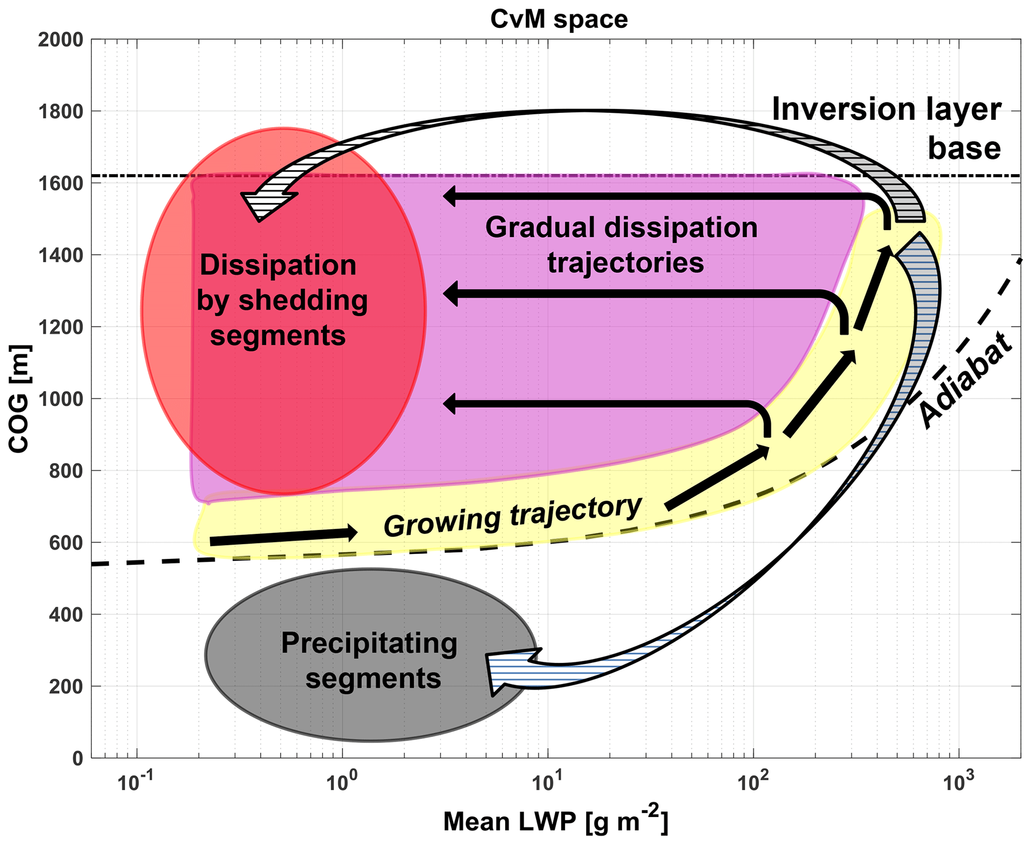
https://www.atmos-chem-phys.net/19/10717/2019/acp-19-10717-2019-f01

Figure 1A schematic representation of a cloud field center-of-gravity height (y axis) vs. mass (x axis) phase space (CvM in short). The majority of clouds are confined to the region between the adiabatic approximation (curved dashed line) and the inversion layer base height (horizontal dashed line). The yellow, magenta, red, and grey shaded regions represent cloud growth, gradual dissipation, cloud fragments which shed large clouds, and cloud fragments which shed precipitating clouds, respectively. The black arrows represent continuous trajectories of cloud growth and dissipation. The hatched arrows represent two possible discontinuous trajectories of cloud dissipation where clouds shed segments.

Download

2.5 Cloud tracking

To follow the evolution of individual clouds within a cloud field, we use an automated 3-D cloud tracking algorithm (see Heiblum et al., 2016a, for details). It enables tracking of continuous cloud entities (CCEs) from formation to dissipation, even if interactions between clouds (splitting or merging) occur during that lifetime. A CCE initiates as a new cloud forming in the field and is tracked under the condition that it retains the majority (>50 %) of its mass during an interaction event with another cloud. Thus, a CCE can terminate due to either cloud dissipation or cloud interactions.

3 Theoretical estimations for different core sizes

Here we propose simple physical considerations to evaluate the differences in cloud partition to core and margin using different definitions. The arguments rely on key findings from previous works (see Sect. 1), with the aim of gaining intuitive understanding of the potential differences between the core types. It is convenient to separate the analysis to an adiabatic case and then add another layer of complexity and consider the effects of mixing of cloudy and non-cloudy air. In this theoretical derivation, saturation adjustment to RH = 100 % is assumed for both cases, while in the other models used in this study, transient supersaturated and sub-saturated cloudy parcels are treated (more realistic).

3.1 Adiabatic case – no mixing

Considering moist-adiabatic ascent, the excess vapor above saturation is instantaneously converted to liquid (saturation adjustment). Thus, the adiabatic cloud is saturated (S=1) throughout its vertical profile, and only W_core and B_core differences can be considered. It is assumed that the adiabatic convective cloud is initiated by positive buoyancy initiating from the sub-cloudy layer. As long as the cloud is growing it should have positive CAPE and will experience positive w throughout the column even if the local buoyancy at a specific height is negative. Eventually the cloud must decelerate due to negative buoyancy and reach a top height, where CAPE = 0 and w=0. Hence, for the adiabatic column case, B_core is always a proper subset of W_core (i.e., B_core ⊂ W_core). These effects are commonly seen in warm convective cloud fields where permanent vertical layers of negative buoyancy (but with updrafts) within clouds typically exist at the bottom and top regions of the cloudy layer (Betts, 1973; de Roode and Bretherton, 2003; Garstang and Betts, 1974; Grant and Lock, 2004; Heus et al., 2009b; Neggers et al., 2007).

3.2 Cloud parcel entrainment model

A mixing model between a saturated (cloudy) parcel and a dry (environment) parcel is used to illustrate the effects of mixing on the different core types. The details of these theoretical calculations are shown in Appendix A. The initial cloudy parcel is assumed to be saturated (part of RH_core), have positive vertical velocity (part of W_core), and experience either positive or negative buoyancy (part of B_core or B_margin), as is seen for the adiabatic column case. Additionally, mixing is assumed to be isobaric and in a steady environment where the average temperature of the environment per a given height does not change. The resultant mixed parcel will have lower humidity content and lower LWC, as compared to the initial cloudy parcel, and a new temperature. In nearly all cases (beside in an extremely humid environment) the mixed parcel will be sub-saturated and evaporation of LWC will occur. Evaporation ceases when equilibrium is reached due to air saturation (S=1) or due to complete evaporation of the droplets (which means S<1, and the mixed parcel is no longer cloudy, since it has no liquid water content).

In addition to mixing between cloudy (core or margin) and non-cloudy parcels, mixing between core and margin parcels (within the cloud) also occurs. This mixing process can be considered to be “entrainment-like” with respect to the cloud core. Considering the changes in the W_core and RH_core, there is no fundamental difference in the treatment of mixing of cloudy and non-cloudy parcels or mixing between core and margin (because the margins and the environment are typically sub-saturated and experience negative vertical velocity). However, for the changes in the B_core after mixing, a fundamental difference exists between mixing with the reference temperature or humidity state (in the case of mixing with the environment) and mixing given a reference temperature or humidity state (in mixing between B_core and B_margin). Thus, it is interesting to check the effects of mixing between B_core and B_margin parcels on the total extent of the B_core with respect to the other two core types. The details of this second case are shown in Appendix B.

3.2.1 Effects of non-cloudy entrainment on buoyancy

When mixed with non-cloudy air, the change in buoyancy of the initial cloudy parcel (which is a part of W_core and RH_core and either B_core or B_margin) happens due to both mixing and evaporation processes. The theoretical calculations show that for all relevant temperatures (∼0 to 30 ^∘C, representing warm Cu), the change in the parcel's buoyancy due to evaporation alone will always be negative (see Appendix A). This is because the negative effect of the temperature decrease outweighs the positive effects of the humidity increase and water loading decrease. Nevertheless, the total change in the buoyancy (due to both mixing and evaporation) depends on the initial temperature, relative humidity, and liquid water content of the cloudy and non-cloudy parcels.

In Fig. A1 in Appendix A a wide range of non-cloudy environmental parcels, each with their own thermodynamic conditions, are mixed with a saturated cloud parcel with either positive or negative buoyancy. The main conclusions regarding the effects of such mixing on the buoyancy are as follows:

To a first order, the initial buoyancy values are temperature dependent, where a cloudy parcel that is warmer (colder) by more than ∼0.2 ^∘C than the environment will be positively (negatively) buoyant for common values of cloudy layer environmental relative humidity (RH > 80 %).
Parcels that are initially part of B_core may only lower their buoyancy due to entrainment; the change results in either to positive or negative buoyancy values, depending on the environmental conditions.
The lower the environmental RH, the larger the probability for parcel transition from B_core to B_margin after entrainment.
Parcels that are initially part of B_margin can either increase or decrease their buoyancy value but never become positively buoyant. The former case (buoyancy decrease) is expected to be more prevalent, since it occurs for the smaller range of temperature differences with the environment.

In summary, entrainment is expected to always have a net negative effect on B_core extent and B_margin values, while evaporation feedbacks serve to maintain RH_core in the cloud. Thus, we can predict that B_core should be a subset of RH_core (i.e., B_core ⊆ RH_core).

3.2.2 Effects of core and margin mixing on buoyancy

We consider the case of mixing between the B_core and B_margin, meaning positively buoyant and negatively buoyant cloud parcels. For simplicity, we assume that both parcels are saturated (S=1; both included in the RH_core). As seen above, such conditions exist in both the adiabatic case and in the case where an adiabatic cloud has undergone some entrainment with the environment. The buoyancy differences between the saturated parcels are mainly due to temperature differences but also due to the increasing saturation vapor pressure with increasing temperature (see Appendix B for details).

In Fig. B1 in Appendix B is it shown that the resultant mixed parcel's buoyancy can be either positive or negative, depending on the magnitude of temperature difference of each parcel (core or margin) from that of the environment. However, in all cases the mixed parcel is supersaturated. This result can be generalized: given two parcels with equal RH but different temperature, the RH of the mixed parcel is always equal to or higher than the initial value. Hence, B_core can either increase or decrease in extent, while the RH_core can only increase due to mixing between saturated B_core and B_margin parcels. This again strengthens the assumption that B_core should be a subset of RH_core.

We note that an alternative option for mixing between the core and margin parcels exists here, in which either or both of the parcels are subsaturated so that the mixed parcel is subsaturated as well. In this case evaporation will also occur. As seen in Appendix A, this should further reduce the buoyancy value of the mixed parcel (while increasing the RH).

3.2.3 Effects of entrainment on vertical velocity

The vertical velocity equation dictates that buoyancy is the main production term (de Roode et al., 2012; Romps and Charn, 2015) and is balanced by perturbation pressure gradients and mixing (on grid and sub-grid scales). Thus, all changes of magnitude (and sign) in vertical velocity should lag the changes in buoyancy. This is the basis of convective overshooting and cumulus formation in the transition layer (see Sect. 3.1). It is interesting to assess the magnitude of this effect by quantifying the expected time lag between buoyancy and vertical velocity changes. The calculations in Appendix A indicate negative buoyancy values reaching −0.1 m s⁻² due to entrainment. However, measurements from within clouds show that the temperature deficiency of cloudy parcels with respect to the environment is generally restricted to less than 1 ^∘C for cumulus clouds (Burnet and Brenguier, 2010; Malkus, 1957; Sinkevich and Lawson, 2005; Wei et al., 1998), and thus the negative buoyancy should be no larger than −0.05 m s⁻². This value is closer to current and previous simulations and also observations that show negative buoyancy values within clouds to be confined between −0.001 and −0.01 m s⁻² (Ackerman, 1956; de Roode et al., 2012).

Given an initial vertical velocity of ∼0.5 m s⁻¹, the deceleration due to buoyancy (and reversal to negative vertical velocity) should occur within a typical time range of 1–10 min. These timescales are much longer than the typical timescales of evaporation (that eliminates the B_core), which range between 1–10 s (Lehmann et al., 2009). Moreover, the fact that a drag force typically balances the buoyancy acceleration (Romps and Charn, 2015) can also contribute to a time lag between effects on buoyancy and subsequent effects on vertical velocity. Therefore, the switching of the sign for vertical velocity should occur with substantial delay compared to the reduction of buoyancy, and B_core should be a subset of W_core (i.e., B_core ⊆ W_core) during the growing and mature stages of a cloud's lifetime.

3.3 The relation between supersaturation and vertical velocity cores

Here we revisit the terms in Eq. (3) to explore an intuitive, first-order understanding of the relation between the vertical velocity core and the supersaturation core. A rising parcel initially has no liquid water content, with its only source of supersaturation being the updraft w, and thus initially the RH_core should always be a subset of W_core. In general, since the sink term $\frac{d q_{l}}{d t}$ becomes a source only when S<1 (the condition for evaporation), the only way for a convective cloud to produce supersaturation (i.e., S>1) is by updrafts during all stages of its lifetime. Once supersaturation is achieved, the sink term becomes positive $\frac{d q_{l}}{d t} > 0$ and balances the updraft source term so that supersaturation either increases or decreases. At any stage, if downdrafts replace the updrafts within a supersaturated parcel, the consequent change in supersaturation becomes strictly negative (i.e., $\frac{d S}{d t} < 0)$ . This negative feedback limits the possibility of finding supersaturated cloudy parcels with downdrafts. Hence, we can expect the RH_core to be smaller than W_core during the majority of a cloud's lifetime.

4 Results – single cloud simulation

The differences between the three types of core definitions are examined during the lifetime of a single cloud (Fig. 2), based on the Hawaiian profile. The cloud's total lifetime is 36 min (between t=7 and t=43 min of simulation). Each panel in Fig. 2 presents vertical cross-sections of the three cores (magenta – W_core, green – RH_core, and yellow – B_core) at four points in time (with 10 min intervals). The cloud has an initial cloud base at 850 m and grows to a maximal top height of 2050 m. The condensation rates (red shades) increase toward the cloud center, and the evaporation rates (blue shades) increase toward the cloud edges. Evaporation at the cloud top results in a large eddy below it that contributes to mixing and evaporation at the lateral boundaries of the cloud. Thus, a positive feedback is initiated which leads to cooling, negative buoyancy, and downdrafts. The dissipation of the cloud is accompanied with a rising cloud base and lowering of the cloud top.

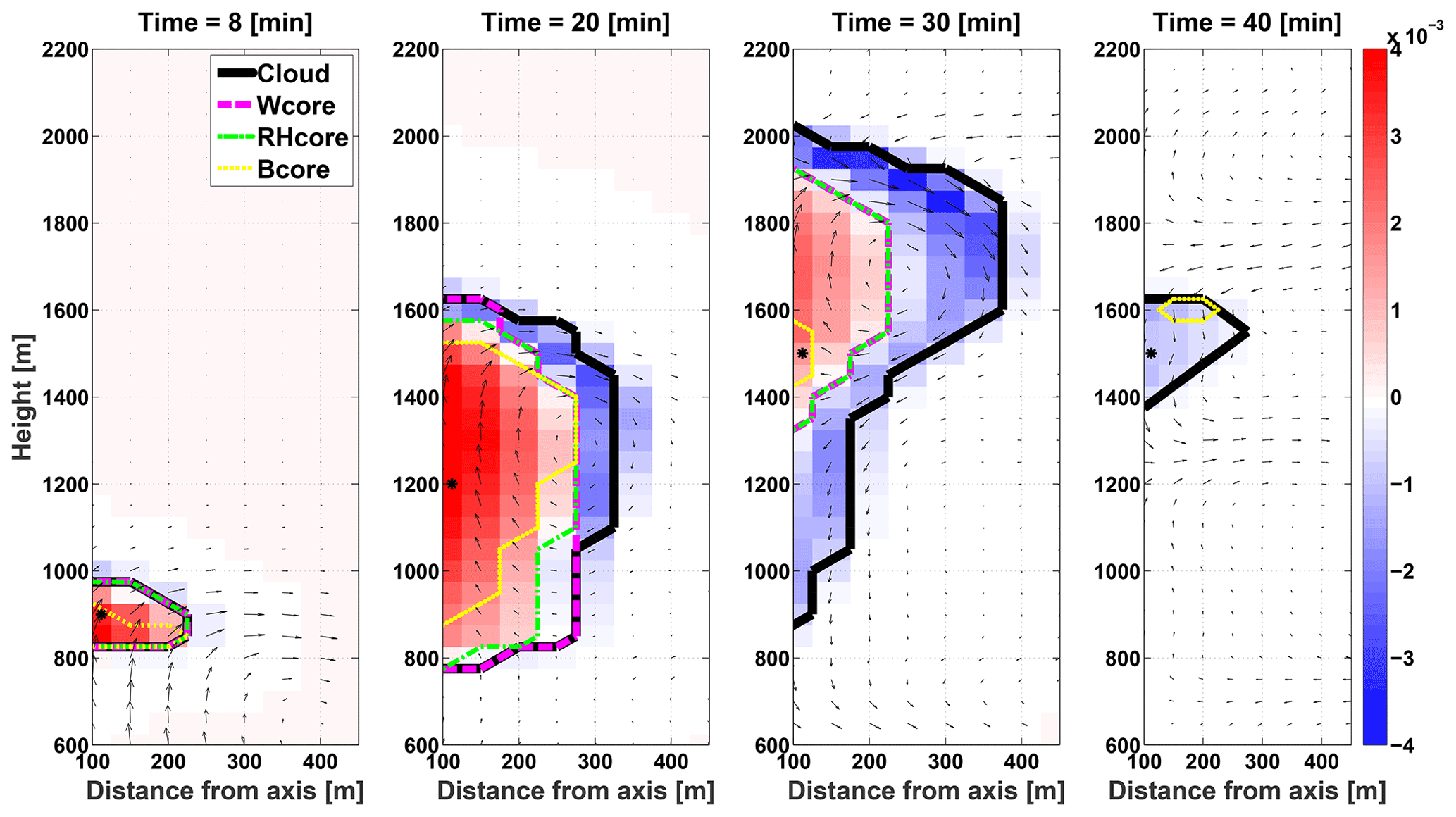
https://www.atmos-chem-phys.net/19/10717/2019/acp-19-10717-2019-f02

Figure 2Four vertical cross-sections (at t=8, 20, 30, and 40 min) during the single cloud simulation. y axis represents height (m), and x axis represents the distance from the axis (m). The black, magenta, green, and yellow lines represent the cloud, W_core, RH_core, and B_core, respectively. The black arrows represent the wind, the background represents the condensation (red) and evaporation rate (blue; g kg⁻¹ s⁻¹), and the black asterisks indicate the vertical location of the cloud centroid. Note that in some cases the lines indicating core boundaries overlap (mainly seen for RH and W cores).

Download

During the growing stage (t=10, 20 min), when substantial condensation still occurs within the cloud, all of the cores seem to be self-contained within one another, with B_core being the smallest and W_core being the largest. During the final dissipation stages, when the cloud shows only evaporation (t=40), W_core and RH_core disappear, while there is still small B_core near the cloud top. Further analysis (see Part 2) shows that the entire dissipating cloud is colder and more humid than the environment, but downdrafts from the cloud top (see arrows in Fig. 2) promote heating, and by that increase the buoyancy in dissipating cloudy pixels, sometimes reaching positive values. These buoyant pockets will be discussed further in Part 2. The results indicate that the three types of physical cores of the cloud are not located around the cloud's geometrical core along the whole cloud lifetime. During cloud growth (i.e., increase in mass and size) the three types of cores surround the cloud's center, while during late dissipation the B_core is offset from the cloud center.

For a more complete view of the evolution of the three core types in the single cloud case, time series of core fractions are shown in Fig. 3. Figure 3a and b show the core liquid mass (core mass ∕ total mass − f_mass) and volume (core volume ∕ total volume – f_vol) fractions out of the cloud's totals. The results are similar for both measures, except for the fact that core mass fractions are larger than core volume fractions. This is due to significantly higher LWC per pixel in the cores compared to the margins, which skews the core mass fraction to higher values. Core mass fractions during the main cloud growing stage (between t=7 and t=27 min simulation time) are around 0.7–0.85, and core volume fractions are around 0.5–0.7. The time series show that as opposed to the W_core and RH_core fractions, which decrease monotonically with time, B_core shows a slight increase during stages of cloud growth. In addition, for most of the cloud's lifetime, the B_core fractions are the smallest and the W_core fractions are the largest, except for the final stage of the clouds dissipation, where downdrafts from the cloud top creates pockets of positive buoyancy. These pockets are located at the cloud's peripheral regions rather than near the cloud's geometrical center as is typically expected for the cloud's core. In the cloud's center (the geometrical core) the B_core is the first one to terminate (at t=32 min) compared to both W_core and RH_core, which decay together (at 36 min).

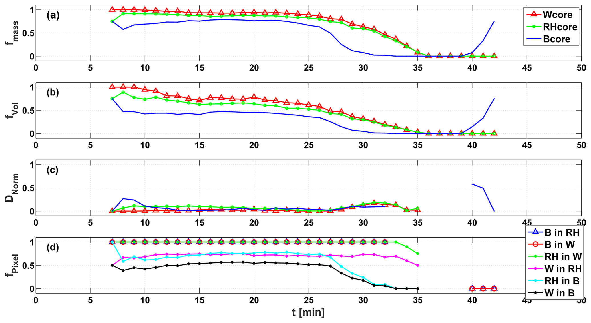
https://www.atmos-chem-phys.net/19/10717/2019/acp-19-10717-2019-f03

Figure 3Temporal evolution of selected core properties, including (a) the fraction of the cores' mass from the total cloud mass (f_mass), (b) the fraction of the cores' volume from the total cloud volume (f_vol), (c) the normalized distance between the cloud centroid and core centroid (D_norm), and (d) the fraction of cores' pixels contained within another core (f_pixel), including all six permutations. See panel legends for descriptions of line colors.

Download

For describing the locations of the physical cores, we examine the normalized distances (D_norm) between the cloud's centroid and the cores' centroids. The evolution of these distances is shown in Fig. 3c. At cloud initiation (t=7 min), when the cloud is very small, all of the cores' centroids coincide with the total cloud centroid location. The B_core (and RH_core to a much lesser degree) centroid then deviates from the cloud centroid to a normalized distance of 0.27 (t=8 min). As cloud growth proceeds, B_core grows and its centroid coincides with the cloud's centroid. All of the cores' centroids are located near the cloud centroid during the majority of the growing and mature stages of the cloud, showing normalized distances <0.1. During dissipation (t>27 min), the cores' centroid locations start to move away from the cloud's geometrical core; this is followed by a reduction in distances due to the rapid loss of cloud volume. As mentioned above, it is shown that the regeneration of positive buoyancy at the end of cloud dissipation (t=40 min) takes place at the cloud edge, with normalized distance >0.5.

Finally, in Fig. 3d the fraction of pixels of each core contained within another core is shown. It can be seen that for the majority of cloud lifetime (up to t=33 min) B_core is a subset (pixel fraction of 1) of RH_core, and the latter is a subset of W_core. As expected, the other three permutations of pixel fractions (e.g., W_core in B_core) show much lower values. The cloudy regions that are not included within B_core but are included within the two other cores are exclusively at the cloud's boundaries (see Fig. 2). The same pattern is seen for cloudy regions that are included within W_core but not in RH_core. During the dissipation stage of the cloud its core subset property (i.e B_core ⊆ RH_core ⊆ W_core) breaks down. Similar temporal evolutions to those shown here are seen for the other simulated clouds (with various aerosol concentrations) in Part 2 of this work.

5 Results – cloud field simulations

5.1 Partition to different core types

To test the robustness of the observed behaviors seen for a single cloud, it is necessary to check whether they also apply to large statistics of clouds in a cloud field. The BOMEX simulation is taken for the analyses here. We discard the first 3 h of cloud field data, during which the field spins up and its mean properties are unstable. In Fig. 4 the volume (f_vol) and mass (f_mass) fractions of the three core types are compared for all clouds (at all output times – every 1 min) in the CvM space. As seen in Fig. 1, the location of specific clouds in the CvM space indicates their stage in evolution. Most clouds are confined to the region between the adiabat and the inversion layer base except for small precipitating (lower-left region) and dissipating clouds (upper-left region). The color shades of the clouds indicate whether a cloud is all core (red – core fraction 1), all margin (blue – core fraction 0), or equally divided into the core and margin (white – core fraction 0.5). The size of each point in the scatter is proportional to the cloud's mean horizontal cross-sectional area. A general increase in mean cloud area with increase in mean cloud LWP is seen (i.e., synchronous growth in the horizontal and vertical axis).

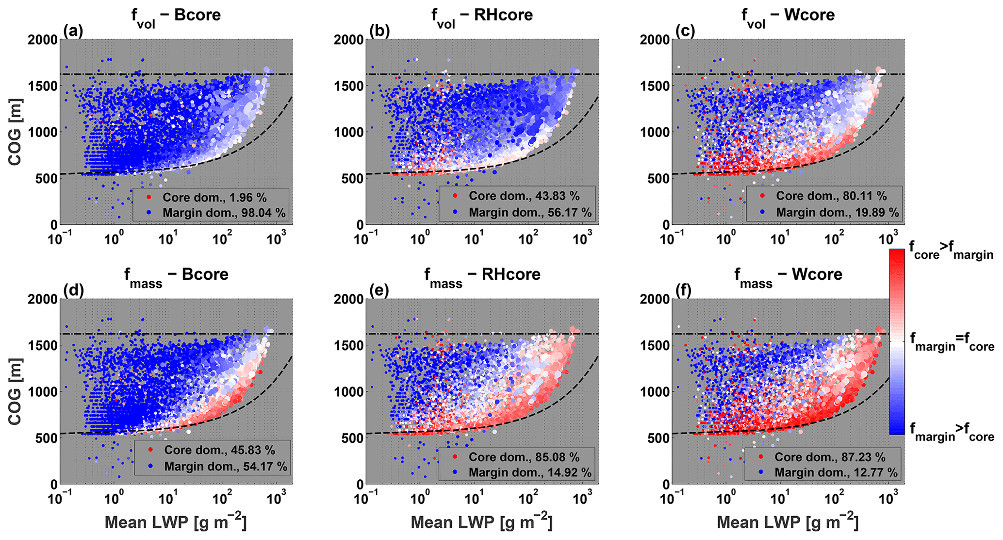
https://www.atmos-chem-phys.net/19/10717/2019/acp-19-10717-2019-f04

Figure 4CvM phase-space diagrams of B_core (a, d), RH_core (b, e), and W_core (c, f) fractions for all clouds between 3 and 8 h in the BOMEX simulation. Both volume fractions (f_vol; a, b, c) and mass fractions (f_mass; d, e, f) are shown. The red (blue) colors indicate a core fraction above (below) 0.5. The size of each point in the scatter is proportional to the cloud mean area, where the smallest (largest) point corresponds to an area of 0.01 (2.36) km². The percentage of clouds that are core dominated (f_volf_mass>0.5) is included in panel legends. For a general description of CvM space characteristics, the reader is referred to Sect. 2.4.

Download

As seen for the single cloud, the core mass fractions tend to be larger than core volume fractions for all core types. This is due to the fact that LWC values in the cloud core regions are higher than in margin regions, so a cloud might be core dominated in terms of mass while being margin dominated in terms of volume. Focusing on the differences between core types, the color patterns in the CvM space imply that B_core definition yields the lowest core fractions (for both mass and volume), followed by RH_core with higher values and W_core with the highest values. The absence of the B_core is especially noticeable for small clouds in their initial growth stages after formation (COG ∼ 550 m and LWP < 1 g m⁻²). Those same clouds show the highest core fractions for the other two core definitions. This large difference can be explained by the existence of the transition layer (as discussed in Sect. 3) near the lifting condensation level (LCL) in warm convective cloud fields, which is the approximated height of a convective cloud base (Craven et al., 2002; Meerkötter and Bugliaro, 2009). Within this layer parcels rising from the sub-cloudy layer are generally colder than parcels subsiding from the cloudy layer. Thus, this transition layer clearly marks the lower edge of the buoyancy core, as most convective clouds are initially negatively buoyant.

Generally, the growing cloud branch (i.e., the CvM region closest to the adiabat) shows the highest core fractions. The RH_core and W_core fractions decrease with cloud growth (increase in mass and COG height), while the B_core initially increases, shows the highest fraction values around the middle region of the growing branch, and then decreases for the largest clouds. The transition from the growing branch to the dissipation branch is manifested by a transition from core-dominated to margin-dominated clouds (i.e., transition from red to blue shades). Mixed within the margin-dominated dissipating cloud branch, a scatter of W_core-dominated small clouds can be seen as well. These represent cloud fragments which shed large clouds during their growing stages with positive vertical velocity. They are sometimes RH_core dominated as well but are strictly negatively buoyant. The few precipitating cloud fragments seen for this simulation (cloud scatter located below the adiabat) tend to be margin dominated, especially for the RH_core.

The percentages in the panel legends (Fig. 4) indicate the fractions of clouds (out of the scatter) which are core dominated with respect to volume or mass. Only ∼2 % of clouds are dominated by B_core in terms of cloud volume, but more than 45 % of the clouds have the majority of their mass within the B_core region. These numbers increase considerably for the RH_core (W_core), where 44 % (80 %) of the clouds are core dominated with respect to cloud volume and 85 % (87 %) of the clouds are core dominated with respect to cloud mass. Thus, the B_core can be considered to be taking up a small portion of a typical cloud mass and volume, while the W_core generally occupies most of the cloud. We note that some of the largest clouds in the field (indicated by large scatter points) show higher (lower) B_core (RH_core and W_core) volume fractions in comparison with smaller clouds located adjacent to them in the CvM phase space. Further analysis shows that these clouds are also precipitating to the surface. The increase in B_core fractions in precipitating clouds is discussed in Part 2 of this work.

5.2 Subset properties of cores

From Fig. 4 it is clear that W_core tends to be the largest and B_core tends to be the smallest. To what degree, however, are the cores subsets of one another as those seen for the single cloud simulation? In Fig. 5 the pixel fraction (f_pixel) of each core type within another core type is shown for all clouds in the CvM space. A f_pixel of 1 (bright colors) indicates that the pixels of the specific core in question (labeled in each panel title) are a subset of the other core (also labeled in the panel title), and a f_pixel of 0 (dark colors) indicates no intersection between the two cores in the cloud. It is seen that B_core tends to be a subset of both other cores, with the f_pixel being around 0.75–1 for most of the growing branch area and large mass dissipating clouds which still have some positive buoyancy. The pixel fractions are higher for B_core inside W_core compared with B_core inside RH_core, but both show a decrease with an increase in growing branch cloud mass, meaning that the chance for finding a proper subset B_core decreases in large clouds.

The CvM space of RH_core inside W_core shows an even stronger relation between these two core types. For almost all growing branch clouds, the RH_core is a subset of W_core (i.e., RH_core ⊆ W_core). The pixel fractions tend to decrease gradually with loss of cloud mass in the dissipation branch. However, some small dissipating clouds show that f_pixel=1. These clouds also experience high core volume fractions (f_vol∼1), as indicated by the scatter point sizes in Fig. 5. The other three permutations of the f_pixel (W_core inside B_core, W_core inside RH_core, and RH_core inside B_core) give an indication of cores' sizes and of which cloud types show no overlap between different cores. As stated above, growing (dissipation) clouds show higher (lower) overlap between the different core types. The W_core is almost twice as large as the B_core and 30 %–40 % larger than the RH_core along most of the growing branch.

https://www.atmos-chem-phys.net/19/10717/2019/acp-19-10717-2019-f05

Figure 5CvM phase-space diagrams of pixel fractions (f_pixel) of each of the three cores within another core, including six different permutations (as indicated in the panel titles). Bright colors indicate high-pixel fractions (large overlap between two core types), while dark colors indicate low-pixel fractions (little overlap between two core types). Only clouds with a non-zero core fraction (for the core in question) are considered (e.g., for the B_core in RH_core in panel a, only clouds that contain at least one pixel with positive buoyancy are considered). Scatter point size is proportional to the minimum f_vol of the core pairs in question.

Download

To give an objective measure of the degree to which different core types can be used interchangeably, we define an interchangeable fraction (f_int), which is the multiplication of the two pixel fractions of a core pair (e.g., $f_{{pixel}_{B in RH}} \cdot f_{{pixel}_{RH in B}}$ ). In Fig. 6 the f_int is shown for all clouds and the three core pairs. It can be seen that only a small percentage (<5 %) of clouds can be considered to have fully interchangeable core types with f_int>0.75. The RH_core–W_core pair shows the highest degree of interchangeability (83 % and 54 % of clouds with f_int>0.25 and f_int>0.5, respectively), showing high f_int for clouds at formation and growing stages and sometimes also late dissipation. The B_core–W_core pair shows the lowest degree of interchangeability (46 % and 6 % of clouds with f_int>0.25 and f_int>0.5, respectively), with mature growing clouds showing the highest f_int values. The B_core–RH_core pair shows similar results, but with slightly higher f_int values on average.

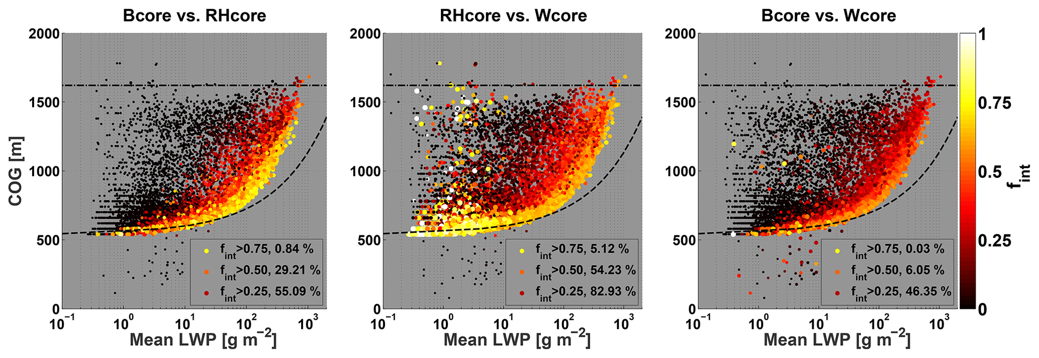
https://www.atmos-chem-phys.net/19/10717/2019/acp-19-10717-2019-f06

Figure 6CvM phase-space diagrams of degree of interchangeability (f_int) for each of the core pairs (as indicated in the panel titles). Bright colors indicate high values (cores can be interchanged with little effect), while dark colors indicate small values (no overlap between cores). Only clouds with a core by at least one definition are considered. Scatter point size is proportional to the minimum f_vol of the core pairs in question. Panel legends include percentage of points (out of the scatter) with f_int above a certain threshold.

Download

5.3 Revisiting the core–shell model

Here we test how well the core–shell model can be applied to the three types of cores in different clouds seen in a warm cumulus cloud field. We test both the location of the cores with respect to the cloud center and horizontal profiles of the three types of core parameters within the cloud. In Fig. 7 the normalized distances between the total cloud centroid and each specific physical core centroid locations (i.e., D_{norm,Centroid}) are evaluated. Since clouds are not always axisymmetric, we also test the distances between total cloud COG and core COG (D_norm,COG), since the COG gives a better representation for where cloud and core mass is concentrated. We take D_norm<0.2 as a threshold for cores located near the centroid or COG and D_norm>0.8 as a threshold for cores located at the cloud edges. For all core types, the large majority of clouds' cores are centered near the clouds' centroid or COG. Only less than 1 % of the clouds' cores reside at the cloud edges, mostly seen for small dissipating clouds. Distances between the cloud COG and core COG yield smaller values than for distances between centroids, implying that the mass is not equally distributed within the clouds, and hence the centroid may be “missing” the true cloud center in terms of mass distribution.

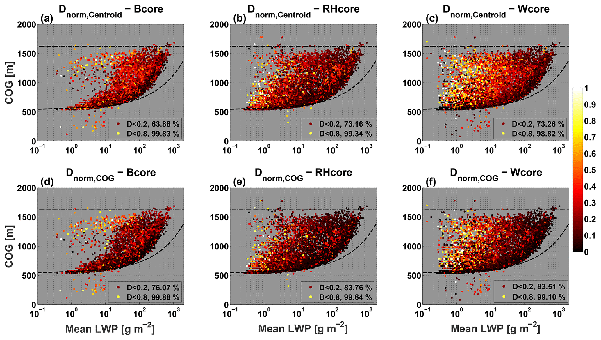
https://www.atmos-chem-phys.net/19/10717/2019/acp-19-10717-2019-f07

Figure 7CvM phase-space diagrams of distances between core centroid and cloud centroid (D_{norm,centroid}; a, b, c), and distances between core COG and cloud COG (D_norm,COG; d, e, f) location, for the three different physical core types. The distances are normalized by the maximum distance between the cloud centroid or COG and the cloud perimeter. Bright (dark) colors indicates large (small) distances. Legends include percentage of points (out of the scatter) with D_norm below a certain threshold. As seen in Fig. 5, only clouds which contain a core fraction above zero (for the core in question) are considered.

Download

Along the growing branch the clouds and physical cores tend to be centered in close proximity, while during cloud dissipation the cores tend to increase in distance from the cloud's center. This type of evolution is most prominent for the W_core, which shows a clear gradient of transition from small (dark colors) to large (bright colors) distances. Focusing on $D_{norm, COG} < 0.2$ , the B_core shows a lower chance of being in proximity to the cloud COG (76 %) than the other core types (83 %). This may be due to a larger prevalence of cloud-edge B_core pixels during dissipation (see Sect. 4 here and Sect. 4.2 in Part 2). Compared to the other clouds, the W_core shows a slightly larger probability of being located at the cloud edge in small dissipating clouds. This can be due to the fact that during cloud dissipation, complex patterns of updrafts and downdrafts within the cloud can create scenarios where the W_core is comprised of very weak updrafts and located anywhere in the cloud.

Further analysis shows that most clouds with $D_{norm, COG} > 0.2$ values can be attributed to the relatively larger-sized clouds which typically contain multiple cores within them (Fig. 8). For the B_core, RH_core, and W_core, 68 %, 79 %, and 81 % of the cloud scatter analyzed (which contains a core) has a single core, respectively. Thus, most clouds have a single core. Moreover, it is more probable to find multiple buoyancy cores in a cloud than vertical velocity cores. This is surprising given our choice of “weak” W_core thresholds (i.e., positive values) and indicates that vertical velocity patterns are relatively well behaved in cumulus clouds, at least for the LES scales chosen here. For clouds with a single core, the growing branch cloud COG and core COG are co-located at the same point. A gradual transition to larger distances is seen as the clouds dissipate to lower mean LWP values. In total, over 80 % of single core clouds have $D_{norm, COG} < 0.2$ for all core types. For clouds with multiple cores, about 50 % of clouds show large distances ( $D_{norm, COG} > 0.2$ ), with little difference between growing branch and dissipating branch clouds. This is to be expected since a large cloud with multiple cores should have a COG somewhere between those cores, explaining the larger normalized distances.

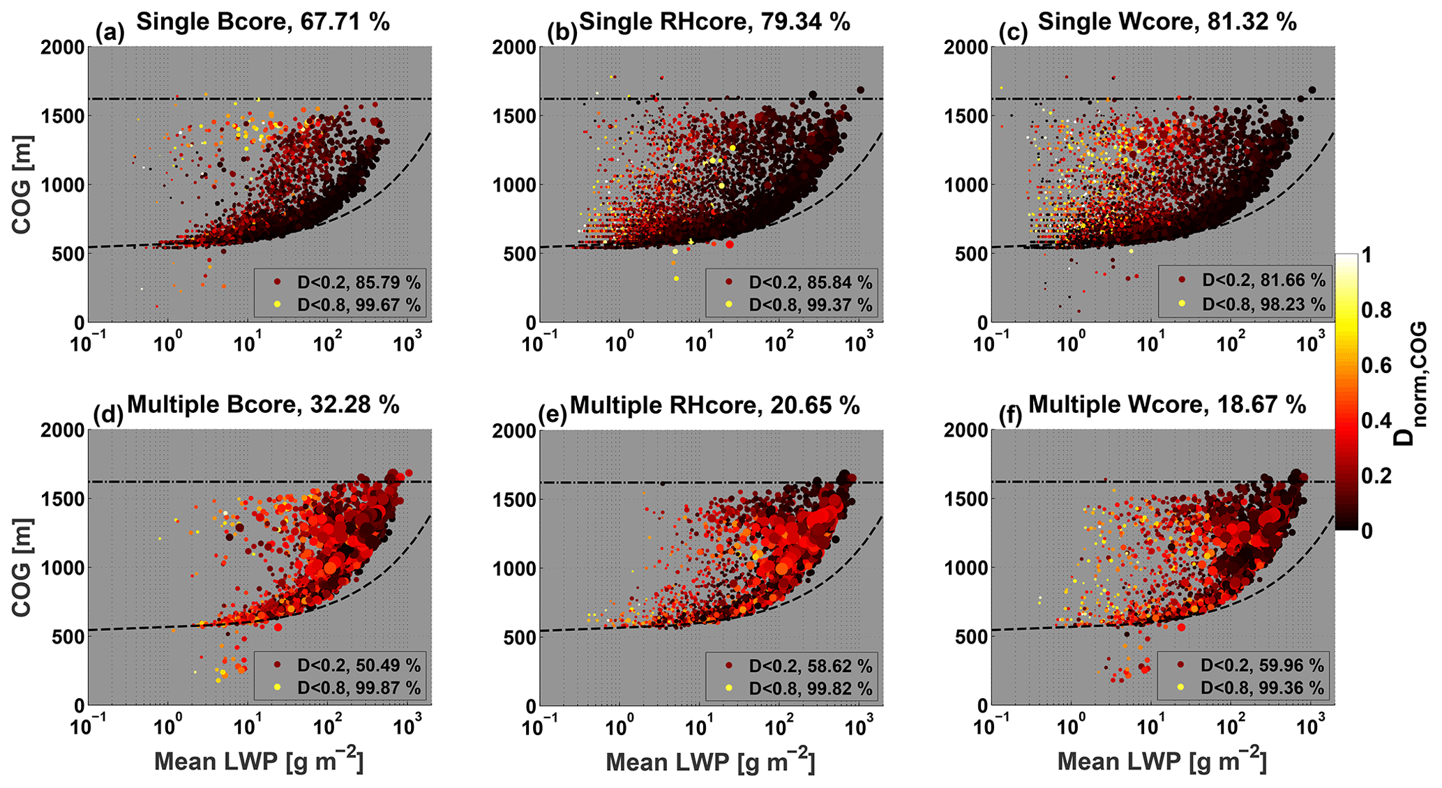
https://www.atmos-chem-phys.net/19/10717/2019/acp-19-10717-2019-f08

Figure 8Same as Fig. 7 but for only distances between core COG and cloud COG (D_norm,COG). Scatter data are partitioned to clouds with a single core (a, b, c) and multiple cores (d, e, f). The size of each point in the scatter is proportional to the cloud mean area.

Download

The core–shell model assumes that the highest values (of a core parameter in question) are located at the center of the cloud (Heus and Jonker, 2008). Is this indeed the case in clouds? In Fig. 9 we observe the likelihood and shape of pre-defined categories of horizontal profiles for core parameters. Profiles are taken along the horizontal plane of the cloud's COG, with distances normalized to cloud maximum horizontal size so that different cloud sizes can be averaged together. Only clouds with at least three pixels in the horizontal plane are taken. Profile categories include the following: (i) core–shell (CS) profiles, which have a positive, maximum value near the COG at $D_{norm, COG} < 0.2$ ; (ii) displaced core–shell profiles (DCS), which have a positive, maximum value somewhere between the COG and periphery at $0.2 < D_{norm, COG} < 0.8$ ; (iii) periphery core (PC) profiles, which have a positive, maximum value at the cloud periphery at $D_{norm, COG} > 0.8$ ; and (iv) no-core (NC) profiles, which are comprised of only negative values. We take only clouds with a single core (or no core), since clouds with multiple cores show more complex profiles that represent a superposition of several single core profiles. The data are further divided to growing and dissipating stages of clouds by checking if a cloud grew in mass compared to the previous time step.

For all core types, there are more single core (and no-core) growing clouds (∼ 55 %–57 %) than dissipating clouds. Generally, it can be seen that the CS category profile is the most prevalent in clouds with single cores, ranging from a maximum of 66 % of growing cloud W_core profiles to a minimum of 26 % of dissipating cloud B_core profiles. As seen in Figs. 4, 7, and 8, growing clouds show a relatively higher percentage of the CS and DCS categories, while dissipation clouds show relatively higher percentages of PC- and NC-category profiles. The W_core and RH_core profiles show similar behavior, with decreasing prevalence from the CS category to the NC category (CS > DCS > PC > NC) for growing clouds. For dissipating clouds, the partition is similar, but with the PC category being the least prevalent (CS > DCS > NC > PC). The main difference in the partition to categories in B_core profiles is the increasing prevalence and dominance of the NC category, as seen in previous analyses. For example, NC profiles are almost non-existent in growing clouds for the W_core and RH_core definitions ( $< = 1$ %) but second-most prevalent using the B_core definition (28 %). Out of the three core types, the W_core shows the highest probability for matching CS and PC categories, the RH_core for the DCS category, and the B_core for the NC category.

On average, the CS category profiles show a monotonic decrease in value from positive to negative values. For growing clouds, vertical velocity may stay positive throughout the horizontal profile, not necessarily showing a downdraft “shell”. The DCS category profiles show positive values from the COG to more than half the cloud size (or the entire cloud size for growing cloud vertical velocity) and have a maximum at D_norm∼0.2, indicating that they are only marginally displaced from the cloud COG. This may indicate that most DCS profiles can actually be considered to be CS profiles, but for clouds with significant asymmetry to the core maximum, they seem to be displaced. Merging of CS and DCS categories comprises 70 %–90 % of all clouds. For both CS and DCS categories, the transition from core to margin (i.e., positive to negative values) occurs at shorter D_norm for dissipating clouds. This transition D_norm value also decreases, gradually moving from the W_core to the RH_core and then to the B_core, indicating smaller core sizes for the latter core types. The NC profiles show little variance with distance from the COG.

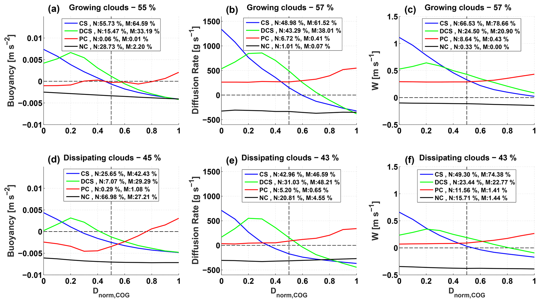
https://www.atmos-chem-phys.net/19/10717/2019/acp-19-10717-2019-f09

Figure 9Mean horizontal profiles of core parameters from the cloud COG to cloud edge, for clouds with single cores and no cores. Data are divided into growing clouds (a, b, c) and dissipating clouds (d, e, f), where the horizontal distances are normalized by the maximum distance to cloud edge. Parameters include buoyancy (a, d), diffusion rate (b, e; taken as a proxy for the supersaturation core), and vertical velocity (c, f). The data are divided to profiles that match core–shell (CS), displaced core–shell (DCS), peripheral core (PC), or no-core (NC) categories, as indicated by the different line colors. The percentages of cloud number (N) and cloud mass (M) attributed to each category are shown in the panel legends. We note that comparing the number percentages with mass percentages for each category gives an indication for the relative sizes of the clouds (e.g., higher N% than M% indicates smaller clouds).

Download

All core (and margin) types show decreasing values moving from growing to dissipating clouds. A decrease in values is also seen when comparing the maximum of the CS, DCS, and PC mean profiles, respectively. An exception is seen for the buoyancy PC category, which shows a slightly higher buoyancy peak value for dissipating clouds. Compared to the RH_core and W_core PC category profiles, which show positive values throughout the cloud (with little change) for smaller-than-average clouds, the B_core PC category shows a transition from margin at the COG to core at the periphery for larger-than-average clouds. This transition to positive buoyancy is even more pronounced (i.e reaches higher values) for dissipating multi-core clouds (not shown here) that tend to be significantly larger. This may indicate that a non-convective process is at play in creating the B_core at the cloud periphery (see Part 2).

5.4 Consistency of the cloud partition to core types

The results for cloud fields are summarized in Fig. 10, which presents the evolution of core fractions of continuous cloud entities (CCEs; see Sect. 2.5 for details) from formation to dissipation. Only CCEs that undergo a complete life cycle are averaged here. These CCEs fulfill the following four conditions: they (i) form near the LCL, (ii) live for at least 10 min, (ii) reach maximum cloud mean LWP values above 10 g m⁻², and (iv) terminate with a mass value below 10 g m⁻². As a test of generality, we performed this analysis for Hawaiian and CASS warm cumulus cloud field simulations in addition to the BOMEX one. For each simulation, hundreds of CCEs are collected (see panel titles), and their core volume fractions are averaged according to their normalized lifetimes (τ).

https://www.atmos-chem-phys.net/19/10717/2019/acp-19-10717-2019-f10

Figure 10Normalized time series of CCE averaged core fractions for the BOMEX (a, b, c), Hawaii (d, e, f), and CASS (g, h, i) simulations. Both core volume fractions (f_vol; a, d, g), normalized distances between cloud and core (D_norm; b, e, h), and pixel fractions of one core within another (f_pixel; c, f, i) are considered. Normalized distance between both COG locations (solid lines) and centroid locations (dotted lines) is shown. Line colors indicated different core types (see legends), while corresponding shaded color regions indicate the standard deviation. Normalized time enables averaging together CCEs with different lifetimes, from formation to dissipation. The number of CCEs averaged together for each simulation is included in the left-column panel titles.

Download

Consistent results are seen for all three simulations. Clouds initiate with a W_core fraction of ∼1, RH_core fraction of ∼0.8, and B_core fraction of ∼0–0.15. The former two core types' volume fraction decreases monotonically with lifetime, while the latter core type's volume fraction increases up to 0.15–0.35 at τ ∼0.3 and then monotonically decreases for increasing τ. The continental (CASS) simulation consistently shows lower buoyancy volume fractions than the oceanic simulations. This can be attributed to lower RH in the CASS cloudy layer (60 %–80 %) compared with the oceanic simulations (85 %–95 %). The lower RH increases entrainment and reduces buoyancy. The fact that clouds end their life cycle with non-zero volume fractions may indicate that some of the CCEs terminate not because of full dissipation but rather because of significant splitting or merging events.

Normalized distances (D_norm) between the CCE core and cloud are also shown in Fig. 10c, f, and i. Both distances between the core centroid (solid lines) and COG (dashed lines) to total cloud centroid and COG are shown. As seen in Fig. 7, D_norm,COG shows smaller values, indicating that the COG indicates the “true” cloud center better compared with the centroid. Distances tend to monotonically increase for RH_core and W_core with the CCE lifetime for all simulations. The gradient of increase is larger at the later stages of the CCE lifetime. Initially the W_core is closer to the geometrical core, but at later stages of the CCE lifetime (typically τ>0.8) this switches and RH_core remains the closest. As seen above, for the first (second) half of the CCE lifetime, the B_core D_norm decreases (increases), starting at normalized distances around 0.2 for all simulations. The physical cores' COG stay closer to the cloud COG (D_norm<0.2) for the majority of their lifetimes for the three cases. Taking again the value $D_{norm, COG} = 0.2$ as a threshold for physical cores centered near the cloud COG, BOMEX, Hawaii, and CASS simulation CCEs' W_core values all cross this threshold at τ=0.9. Thus, the core–shell geometrical model is true for about 90 % of a typical cloud's lifetime.

The analysis of core subset properties (Fig. 10c, f, i) shows that the assumption B_core ⊆ RH_core ⊆ W_core is true for the initial formation stages of a cloud. Although the corresponding pixel fractions decrease slightly during the lifetime of the CCE, they remain above 0.9 (e.g., B_core is 90 % contained within RH_core). A sharp decrease in pixel fractions is seen for τ>0.8 (τ>0.5 for the CASS simulation), as the overlaps between the different cores are reduced during dissipation stages of the cloud. For all simulations, the highest pixel fraction values are seen for the B_core inside the W_core pair, followed by RH_core inside the W_core pair and B_core inside the RH_core pair, showing lower values. In addition, it can be seen that the variance of the average pixel fraction (per τ) increases with an increase in τ. This is due to the fact the all CCEs initiate with almost identical characteristics but may terminate in very different ways. In Part 2 of this work we show that this variance is highly influenced from precipitation, which contributes to more significant interactions between clouds (Heiblum et al., 2016b).

6 Summary

In this paper we study the partition of warm convective clouds to core and margin according to three different definitions: (i) positive vertical velocity (W_core), (ii) relative humidity supersaturation (RH_core), and (iii) positive buoyancy (B_core), with emphasis on the differences between those definitions. Using theoretical considerations of both an adiabatic cloud column and a simple two-parcel mixing model (see Appendices A and B), we support our simulated results, as we show that the B_core is expected to be the smallest of the three. This finding is in line with previous works that showed that negative buoyancy is prevalent in cumulus clouds for a wide range of thermodynamic conditions (de Roode, 2007; Paluch, 1979; Taylor and Baker, 1991). This is due to the fact that entrainment into the core (i.e., mixing with non-cloudy environment or mixing with the margin regions of the cloud) may result in sub-saturation, followed by evaporation that always has a negative net effect on buoyancy. The same process has an opposing effect on the relative humidity of the mixed parcel and acts to reach saturation. Entrainment (or mixing) also acts to decrease vertical velocity but at slower manner compared to the timescales of changes in the buoyancy and relative humidity. In addition, the supersaturation equation (Eq. 3) predicts that it is unlikely to maintain supersaturation in a cloudy volume with negative vertical velocity. Hence, W_core can be expected to be the largest of the three cores.

Using numerical simulations of both a single cloud and cloud fields of warm cumulus clouds, we show that during most stages of clouds' lifetime, W_core is indeed the largest of the three and B_core is the smallest. Only 2 % of clouds are dominated (in volume fraction) by the B_core, while 44 % and 83 % of clouds are dominated by RH_core and W_core, respectively. The warm convective cloud fields simulated here typically have a transition layer near the lifting condensation level (LCL). Thus, the lower parts of the clouds are negatively buoyant or even lack B_core at formation. After cloud formation, internal growth processes (i.e., condensation and latent heat release) increase the B_core until dissipation processes become dominant and the B_core decreases quickly due to entrainment. In contrast, clouds are initially dominated by the W_core and RH_core (fractions close to 1). The fractions of these cores then decrease monotonically with cloud lifetime.

During dissipation stages, the clouds are mostly margin dominated such that most of the small mass dissipation cloud fragments are entirely coreless. However, several small mass dissipating cloud fragments which shed large cloud entities (with large COG height) may be core dominated, especially when using the vertical velocity core definition. The same is observed for small precipitating cloud fragments which reside below the convective cloud base. We note that the results here are similar for both volume and mass core fractions out of the cloud's total fraction, with the core mass fractions being larger due to a skewed distribution of cloud LWC which favors the core regions. Moreover, we show that these results are consistent for various levels of aerosol concentrations (will be seen in Part 2) and different thermodynamic profiles used to initialize the models.

In addition to the differences in their sizes, the three cores tend to be subsets of one another in the following order: B_core ⊆ RH_core ⊆ W_core. This property is most valid for a cloud at its initial stages and breaks down gradually during a cloud's lifetime. The decrease in overlap between different core types during dissipation implies that minor local effects enable core existence rather than cloud convection. Only during growth and mature stages can the three core definitions be used interchangeably with the least amount of difference in core sizes. Generally, the RH_core–W_core pair are most interchangeable, while the B_core–W_core pair are the least interchangeable.

With respect to cloud morphology, the majority of clouds are composed from single cores (for all core types), are located near the cloud centroid and COG, and fit the intuitive core–shell model of decreasing core parameter values from the cloud center to periphery. This is especially true during cloud growth, as during dissipation the cores may decouple from the geometrical core and often comprise just a few isolated pixels at the cloud's edges. In terms of cloud lifetime, the core–shell model applies to at least 80 % of a typical cumulus cloud lifetime. We note that using the COG as a measure for the cloud and core geometrical centers yields smaller cloud–core distances than their centroids. Thus, the COG better represents the cloud physical center. Out of the three core types, the W_core (B_core) shows the highest (lowest) chance of being a single core in the cloud. This is despite choosing a low W_core threshold of W>0. Relatively large clouds tend to have multiple cores so that the mean (mass weighted) core COG location is displaced from the cloud COG. The B_core COG shows the highest chance to be located away from the cloud COG. In some cases of larger clouds, the buoyancy horizontal profile may look exactly opposite to the core–shell one (i.e., maximum at the periphery and minimum at the center). This may be due to downdraft-induced heating at the clouds' edge that promotes positive buoyancy (see more in Part 2). In Part 2 of this work we use the insights gained here on clouds' partition to its core and margin to understand aerosol effects on warm convective clouds.

Data availability

The microphysical and thermo-dynamical profiles used to initialize the single cloud and cloud field numerical simulations can be obtained upon request from the corresponding author.

Appendix A: Buoyancy changes due to mixing of cloudy and non-cloudy parcels

Here we present a simple model for entrainment mixing between a cloudy parcel (either part of B_core or B_margin) and a dry environmental parcel. Entrainment mixes the momentum, heat, and humidity of the two parcels. We consider the mixing of a unit mass of cloud parcel which is defined by two criteria:

\begin{array}{l} S_{1} \geq 1, \\ B_{1} > 0 or B_{1} < 0, \end{array}

with a unit mass of dry environment parcel, defined by

S_{2} < 1,

and explore the properties of the resulting mixed parcel.

Assume that T₁, T₂, T₃ are the initial temperatures of the cloudy, environmental, and resulting mixed parcel, respectively. $q_{v_{1}}$ , $q_{v_{2}}$ , $q_{v_{3}}$ , θ₁, θ₂, θ₃, and $q_{l_{1}}$ , $q_{l_{2}}$ , $q_{l_{3}}$ are their respective vapor mixing ratios, potential temperatures, and liquid water contents (LWC).

The change in buoyancy due to mixing will be

\begin{matrix} (A1) & d B_{mix} = g \cdot (\frac{θ_{3} - θ_{1}}{θ_{2}} + 0.61 (q_{v_{3}} - q_{v_{1}}) - (q_{l_{3}} - q_{l_{1}})), \end{matrix}

with

\begin{matrix} (A2) & T_{3} = μ_{1} \cdot T_{1} + μ_{2} \cdot T_{2}, \\ (A3) & q_{v_{3}} = μ_{1} \cdot q_{v_{1}} + μ_{2} \cdot q_{v_{2}}, \\ (A4) & q_{l_{3}} = μ_{1} \cdot q_{l_{1}} + μ_{2} \cdot q_{l_{2}}, \end{matrix}

where μ₁ and μ₂ are the corresponding mixing fractions. We assume that the mixed parcel is at the same height as the cloudy and environmental parcels and that the mean environmental temperature at that height stays the same after mixing. The potential temperature (θ) is calculated using its definition.

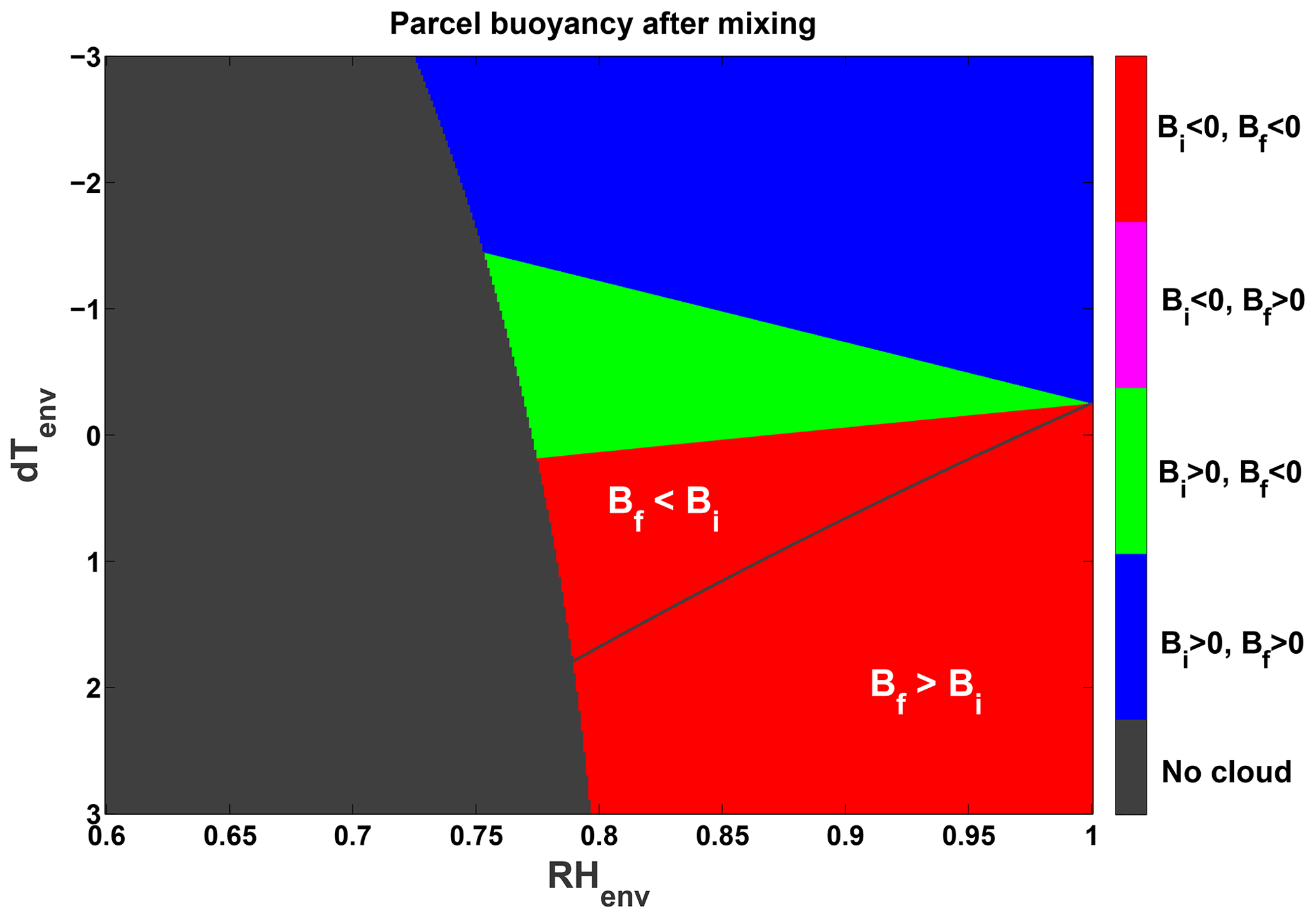
https://www.atmos-chem-phys.net/19/10717/2019/acp-19-10717-2019-f11

Figure A1Phase space presenting the effects of entrainment on cloud buoyancy, where the initial cloudy parcel buoyancy (B_i) and final mixed parcel buoyancy (B_f) are considered. A mixing fraction of 0.5 is chosen. The initial cloudy parcel is saturated (S=1) and has a temperature of 15 ^∘C, pressure of 850 mbar, and LWC of 1 g kg⁻¹. The x axis spans a range of environmental relative humidity values (RH_env), and the y axis has a temperature difference ( $d T_{env} = T_{env} - T_{cld}$ ) range between the cloud and the environment parcels. Red color represents B_i<0 and B_f<0 (i.e., parcel stays negatively buoyant after the mixing), magenta represents B_i<0 and B_f>0 (i.e., transition from negative to positive buoyancy), green represents B_i>0 and B_f<0 (i.e., transition from positive to negative buoyancy), and blue represents B_i>0 and B_f>0 (i.e., parcel stays positively buoyant). The grey color represents mixed parcels that were depleted from water (LWC value lower than 0.01 g kg⁻¹) after evaporation and are considered to be non-cloudy. The white line separates between areas where B_f>B_i and B_f<B_i.

Download

After the mixing process, the resultant mixed parcel may be subsaturated (S₃<1), and cloud droplets start to evaporate. The evaporation process increases the humidity of the parcel. Korolev et al. (2016, Eq. A8) calculated the amount of the required liquid water for evaporation in order to reach S=1 again:

\begin{matrix} (A5) & δ q = \frac{C_{p} R_{v} T_{2}^{2}}{L^{2}} \ln (\frac{1 + \frac{e_{s} (T_{3}) R_{a} L^{2}}{P C_{p} R_{v}^{2} T_{3}^{2}}}{1 + S_{3} \frac{e_{s} (T_{3}) R_{a} L^{2}}{P C_{p} R_{v}^{2} T_{3}^{2}}}), \end{matrix}

where C_p is a specific heat at constant pressure, e_s(T₃) is the saturated vapor pressure for the mixed temperature, P is pressure, L is latent heat, and R_v, R_a are individual gas constants for water vapor and dry air, respectively. If the mixed parcel contains sufficient LWC to evaporate a δq amount of water, the mixed parcel will reach saturation. We note that Eq. (A5) holds for cases where $|T_{1} - T_{2}| < 10$ ^∘C, which is well within the range seen in our simulations of warm clouds.

Assuming that the average environmental temperature stays the same after evaporation, the buoyancy after evaporation is calculated using the following formulas:

\begin{matrix} (A6) & d B_{evap} = g \cdot (\frac{d θ_{evap}^{'}}{θ_{2}} + 0.61 d q_{v_{evap}} - d q_{l_{evap}}), \\ (A7) & d θ_{evap}^{'} = d T_{evap}, \end{matrix}

and from the first law of thermodynamics,

\begin{matrix} (A8) & C_{p} \cdot d T_{evap} = - L \cdot d q_{v_{evap}} . \end{matrix}

The water vapor is the amount of liquid water lost by evaporation:

\begin{matrix} (A9) & d q_{v_{evap}} = - d q_{l_{evap}} = δ q . \end{matrix}

From the equation above, we get

\begin{matrix} (A10) & d B_{evap} = g \cdot δ q (1.61 - \frac{L}{C_{p} θ_{2}}) . \end{matrix}

For a wide temperature range between 200≪300 (K), dB_evap is always negative. This result is not trivial because evaporation both decreases the T and increases the q_v, which have opposite effects. The total change in buoyancy is taken as the sum of dB_evap and dB_mix.

Figure A1 presents a phase space of possible changes in cloudy pixel buoyancy due to mixing with outside air, for various thermodynamic conditions, and a mixing fraction of 0.5. The initial cloudy parcel is chosen to be saturated (S=1) and includes an LWC of 1 g kg⁻¹. The pressure is assumed to be 850 mbar, and the temperature is assumed to be 15 ^∘C. However, we note that the conclusions here apply to all atmospherically relevant values of pressure, temperature, supersaturation (values of RH > 100 %), and the LWC in warm clouds. The x axis in Fig. A1 spans a range of non-cloudy environmental relative humidity values (60 % < RH < 100 %), and the y axis spans a temperature difference range between the cloud and the environment parcels ( $- 3^{\circ} < d T < 3^{\circ}$ ). The initial (B_i) and final (B_f; after entrainment) buoyancy values and the differences between them can be either positive or negative. The regions of B_i>0 (B_i<0) in fact illustrate the effects of entrainment on B_core (B_margin) parcels.

Appendix B: Buoyancy changes due to mixing of core and margin parcels

Following the notations of Appendix A, we now consider the mixing of two cloudy parcels, one part of B_core and one part of B_margin. For simplicity, we choose the case where both parcels are saturated and have the same LWC of 0.5 g kg⁻¹:

\begin{matrix} (B1) & \begin{array}{l} S_{core} = S_{margin} = S_{cloud} = 1, \\ q_{l_{core}} = q_{l_{margin}} = q_{l_{cloud}} = 0.5 . \end{array} \end{matrix}

The buoyancy of each cloudy parcel is determined in reference to the environmental temperature and humidity, $T_{env} q_{v_{env}}$ , so that

\begin{matrix} (B2) & B_{cloud} = g \cdot (\frac{θ_{cloud} - θ_{env}}{θ_{env}} + 0.61 (q_{v_{cloud}} - q_{v_{env}}) - q_{l_{cloud}}) . \end{matrix}

As mentioned in the main text, we take a temperature range of $T_{env} - 3^{\circ} C < T_{cloud} < T_{env} + 3^{\circ} C$ . Each cloudy parcel's temperature also dictates its saturation vapor pressure e_s(T_cloud) and therefore also its humidity content, $q_{v_{cloud}}$ . Plugging these into Eq. (B2), one can associate each temperature–humidity pair with the B_core or B_margin:

\begin{matrix} (B3) & \begin{aligned} T_{core} & = T_{cloud} (B_{cloud} > 0), \\ q_{v_{core}} & = q_{v_{cloud}} (B_{cloud} > 0), \\ T_{margin} & = T_{cloud} (B_{cloud} < 0), \\ q_{v_{margin}} & = q_{v_{cloud}} (B_{cloud} < 0) . \end{aligned} \end{matrix}

The core and margin parcels can then be mixed (see Appendix A), yielding a mixed parcel temperature and humidity content and thus a new relative humidity. The buoyancy of the mixed parcel is obtained by inserting these parameters in Eq. (B2).

In Fig. B1 the resultant buoyancy values and RH values after the mixing of B_core parcels with B_margin parcels are shown. As defined in Appendix A, temperature differences between the parcels and the environment are confined to ±3 ^∘C. The reference environmental temperature, pressure, and RH are taken to be 15 ^∘C, 850 mbar, and 90 %, respectively. We note the main differences between this section and Appendix A are the absence of evaporation and the fact that the core and margin thermodynamic variables are the ones that vary while the reference environmental ones are kept constant.

It can be seen that all negatively buoyant parcels are colder than the environment and nearly all positively buoyant parcels are warmer than the environment, except for a small fraction of them that are slightly colder but positively buoyant due to the increased humidity. The transition from B_f>0 to B_f<0 near the 1-to-1 line indicates that B_f is approximately linearly dependent on the temperature differences with respect to the environment. In other words, if $|T_{core} - T_{env}| > |T_{margin} - T_{env}|$ , the mixed parcel is expected to be part of the B_core (i.e., B_f>0). The exponential increase in saturation vapor pressure with temperature is demonstrated by the results of the mixed parcel final RH, which all show supersaturation values. Additional sensitivity tests were performed for this analysis, showing only weak dependencies on environmental parameter values while maintaining the main conclusions.

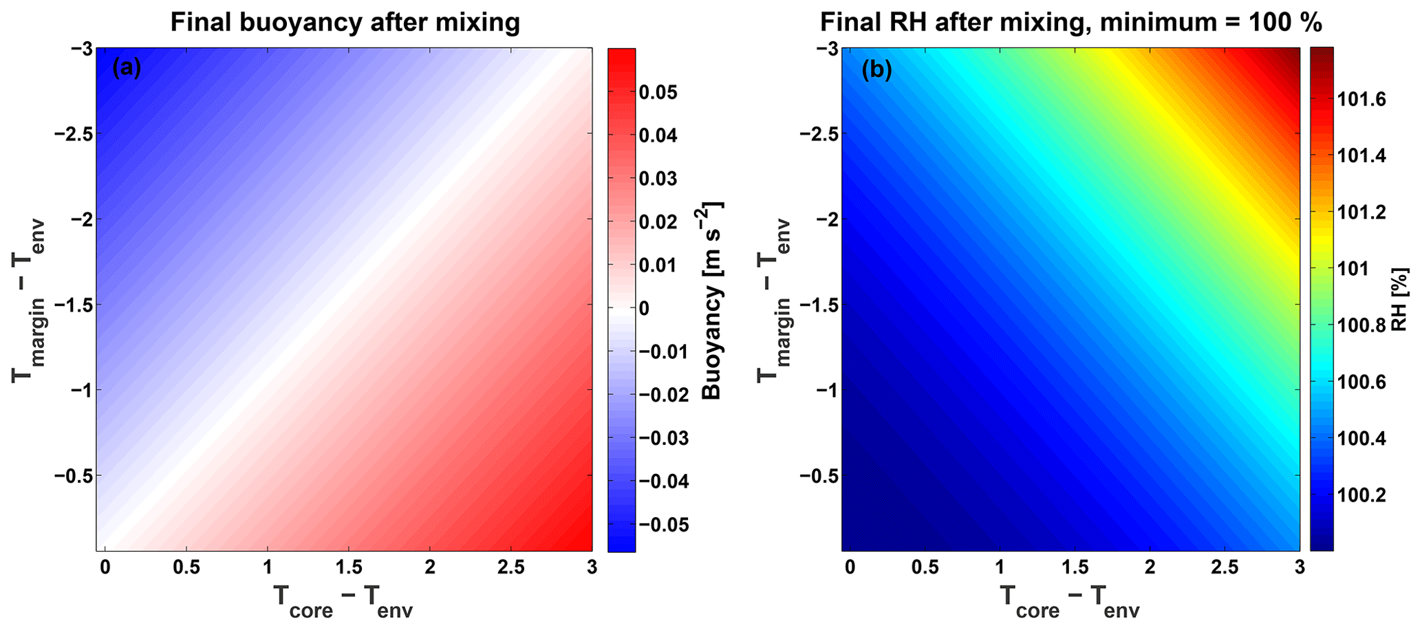
https://www.atmos-chem-phys.net/19/10717/2019/acp-19-10717-2019-f12

Figure B1Phase space presenting the resultant buoyancy (a) and relative humidity (RH; b) when mixing B_core and B_margin parcels with equal RH but different temperatures. A mixing fraction of 0.5 is chosen. Both parcels are initially saturated (RH = 100 %) and have an LWC of 0.5 g kg⁻¹. The environment has a temperature of 15 ^∘C and pressure of 850 mbar. The x(y) axis spans the range of temperature differences between the B_core (B_margin) parcel and the environment.

Download

Author contributions

RHH formulated the theoretical arguments, ran cloud field simulations and conducted the analyses, and wrote the final draft of paper. LP participated in writing the first draft and performed single cloud simulations and relevant analyses. OA, GD, and IK participated in paper editing and discussions.

Competing interests

The authors declare that they have no conflict of interest.

Acknowledgements

The authors would like to acknowledge the Weizmann Institute High Performance Computing (HPC) team for their support.

Financial support

This research has been supported by the Ministry of Science and Technology, Israel (grant no. 3-14444).

Review statement

This paper was edited by Eric Jensen and reviewed by two anonymous referees.

References

Ackerman, B.: Buoyancy and precipitation in tropical cumuli, J. Meteorol., 13, 302–310, https://doi.org/10.1175/1520-0469(1956)013<0302:BAPITC>2.0.CO;2, 1956.

Altaratz, O., Koren, I., Reisin, T., Kostinski, A., Feingold, G., Levin, Z., and Yin, Y.: Aerosols' influence on the interplay between condensation, evaporation and rain in warm cumulus cloud, Atmos. Chem. Phys., 8, 15–24, https://doi.org/10.5194/acp-8-15-2008, 2008.

Betts, A. K.: Non-precipitating cumulus convection and its parameterization, Q. J. Roy. Meteor. Soc., 99, 178–196, https://doi.org/10.1002/qj.49709941915, 1973.

Burnet, F. and Brenguier, J.-L.: The onset of precipitation in warm cumulus clouds: An observational case-study, Q. J. Roy. Meteor. Soc., 136, 374–381, https://doi.org/10.1002/qj.552, 2010.

Craven, J. P., Jewell, R. E., and Brooks, H. E.: Comparison between Observed Convective Cloud-Base Heights and Lifting Condensation Level for Two Different Lifted Parcels, Weather Forecast., 17, 885–890, https://doi.org/10.1175/1520-0434(2002)017<0885:CBOCCB>2.0.CO;2, 2002.

Dagan, G., Koren, I., and Altaratz, O.: Competition between core and periphery-based processes in warm convective clouds – from invigoration to suppression, Atmos. Chem. Phys., 15, 2749–2760, https://doi.org/10.5194/acp-15-2749-2015, 2015.

Dawe, J. T. and Austin, P. H.: The influence of the cloud shell on tracer budget measurements of LES cloud entrainment, J. Atmos. Sci., 68, 2909–2920, https://doi.org/10.1175/2011JAS3658.1, 2011.

Dawe, J. T. and Austin, P. H.: Statistical analysis of an LES shallow cumulus cloud ensemble using a cloud tracking algorithm, Atmos. Chem. Phys., 12, 1101–1119, https://doi.org/10.5194/acp-12-1101-2012, 2012.

de Roode, S. R.: Thermodynamics of cumulus clouds, Física de la Tierra, Vol. 19, Universidad Complutense de Madrid, 2007.

de Roode, S. R. and Bretherton, C. S.: Mass-Flux Budgets of Shallow Cumulus Clouds, J. Atmos. Sci., 60, 137–151, https://doi.org/10.1175/1520-0469(2003)060<0137:MFBOSC>2.0.CO;2, 2003.

de Roode, S. R., Siebesma, A. P., Jonker, H. J. J., and de Voogd, Y.: Parameterization of the vertical velocity equation for shallow cumulus clouds, Mon. Weather Rev., 140, 2424–2436, https://doi.org/10.1175/MWR-D-11-00277.1, 2012.

de Rooy, W. C. and Siebesma, A. P.: A simple parameterization for detrainment in shallow cumulus, Mon. Weather Rev., 136, 560–576, https://doi.org/10.1175/2007MWR2201.1, 2008.

Derbyshire, S. H., Maidens, A. V., Milton, S. F., Stratton, R. A., and Willett, M. R.: Adaptive detrainment in a convective parametrization, Q. J. Roy. Meteor. Soc., 137, 1856–1871, https://doi.org/10.1002/qj.875, 2011.

Emanuel, K. A.: A Scheme for Representing Cumulus Convection in Large-Scale Models, J. Atmos. Sci., 48, 2313–2329, https://doi.org/10.1175/1520-0469(1991)048<2313:ASFRCC>2.0.CO;2, 1991.

Feingold, G., Tzivion, S., and Levin, Z.: Evolution of raindrop spectra. part I: solution to the stochastic collection/breakup equation using the method of moments, J. Atmos. Sci., 45, 3387–3399, https://doi.org/10.1175/1520-0469(1988)045<3387:EORSPI>2.0.CO;2, 1988.

Feingold, G., Levin, Z., and Tzivion, S.: The evolution of raindrop spectra. part III: downdraft generation in an axisymmetrical rainshaft model, J. Atmos. Sci., 48, 315–330, https://doi.org/10.1175/1520-0469(1991)048<0315:TEORSP>2.0.CO;2, 1991.

Garstang, M. and Betts, A. K.: A review of the tropical boundary layer and cumulus convection: structure, parameterization, and modeling, B. Am. Meteorol. Soc., 55, 1195–1205, https://doi.org/10.1175/1520-0477(1974)055<1195:AROTTB>2.0.CO;2, 1974.

Grabowski, W. W. and Jarecka, D.: Modeling condensation in shallow nonprecipitating convection, J. Atmos. Sci., 72, 4661–4679, https://doi.org/10.1175/JAS-D-15-0091.1, 2015.

Grant, A. L. M. and Lock, A. P.: The turbulent kinetic energy budget for shallow cumulus convection, Q. J. Roy. Meteorol. Soc., 130, 401–422, https://doi.org/10.1256/qj.03.50, 2004.

Gregory, D. and Rowntree, P. R.: A Mass Flux Convection Scheme with Representation of Cloud Ensemble Characteristics and Stability-Dependent Closure, Mon. Weather Rev., 118, 1483–1506, https://doi.org/10.1175/1520-0493(1990)118<1483:AMFCSW>2.0.CO;2, 1990.

Hannah, W. M.: Entrainment versus Dilution in Tropical Deep Convection, J. Atmos. Sci., 74, 3725–3747, https://doi.org/10.1175/JAS-D-16-0169.1, 2017.

Heiblum, R. H., Altaratz, O., Koren, I., Feingold, G., Kostinski, A. B., Khain, A. P., Ovchinnikov, M., Fredj, E., Dagan, G., Pinto, L., Yaish, R., and Chen, Q.: Characterization of cumulus cloud fields using trajectories in the center of gravity versus water mass phase space: 1. Cloud tracking and phase space description, J. Geophys. Res.-Atmos., 121, 6336–6355, https://doi.org/10.1002/2015JD024186, 2016a.

Heiblum, R. H., Altaratz, O., Koren, I., Feingold, G., Kostinski, A. B., Khain, A. P., Ovchinnikov, M., Fredj, E., Dagan, G., Pinto, L., Yaish, R., and Chen, Q.: Characterization of cumulus cloud fields using trajectories in the center of gravity versus water mass phase space: 2. Aerosol effects on warm convective clouds, J. Geophys. Res.-Atmos., 121, 6356–6373, https://doi.org/10.1002/2015JD024193, 2016b.

Heiblum, R. H., Pinto, L., Altaratz, O., Dagan, G., and Koren, I.: Core and margin in warm convective clouds – Part 2: Aerosol effects on core properties, Atmos. Chem. Phys., 19, 10739–10755, https://doi.org/10.5194/acp-19-10739-2019, 2019.

Hernandez-Deckers, D. and Sherwood, S. C.: A numerical investigation of cumulus thermals, J. Atmos. Sci., 73, 4117–4136, https://doi.org/10.1175/JAS-D-15-0385.1, 2016.

Heus, T. and Jonker, H. J. J.: Subsiding Shells around Shallow Cumulus Clouds, J. Atmos. Sci., 65, 1003–1018, https://doi.org/10.1175/2007JAS2322.1, 2008.

Heus, T. and Seifert, A.: Automated tracking of shallow cumulus clouds in large domain, long duration large eddy simulations, Geosci. Model Dev., 6, 1261–1273, https://doi.org/10.5194/gmd-6-1261-2013, 2013.

Heus, T., Pols, C. F. J., Jonker, H. J. J., Van den Akker, H. E. A., and Lenschow, D. H.: Observational validation of the compensating mass flux through the shell around cumulus clouds, Q. J. Roy. Meteor. Soc., 135, 101–112, https://doi.org/10.1002/qj.358, 2009a.

Heus, T., Jonker, H. J. J., Van den Akker, H. E. A., Griffith, E. J., Koutek, M., and Post, F. H.: A statistical approach to the life cycle analysis of cumulus clouds selected in a virtual reality environment, J. Geophys. Res., 114, D06208, https://doi.org/10.1029/2008JD010917, 2009b.

Holland, J. Z. and Rasmusson, E. M.: Measurements of the Atmospheric Mass, Energy, and Momentum Budgets Over a 500-Kilometer Square of Tropical Ocean, Mon. Weather Rev., 101, 44–55, https://doi.org/10.1175/1520-0493(1973)101<0044:MOTAME>2.3.CO;2, 1973.

IPCC: Climate Change 2013: The Physical Science Basis. Working Group I Contribution to the Fifth Assessment Report of the IPCC, Cambridge Univ. Press, New York, 2013.

Jaenicke, R.: 9.3.1 Physical properties, in: Physical and chemical properties of the air, edited by: Fischer, G., 405–420, Springer-Verlag, Berlin/Heidelberg, 1988.

Jiang, H. and Feingold, G.: Effect of aerosol on warm convective clouds: Aerosol-cloud-surface flux feedbacks in a new coupled large eddy model, J. Geophys. Res., 111, D01202, https://doi.org/10.1029/2005JD006138, 2006.

Jonker, H. J. J., Heus, T., and Sullivan, P. P.: A refined view of vertical mass transport by cumulus convection, Geophys. Res. Lett., 35, L07810, https://doi.org/10.1029/2007GL032606, 2008.

Kain, J. S. and Fritsch, J. M.: A One-Dimensional Entraining/Detraining Plume Model and Its Application in Convective Parameterization, J. Atmos. Sci., 47, 2784–2802, https://doi.org/10.1175/1520-0469(1990)047<2784:AODEPM>2.0.CO;2, 1990.

Khain, A., Pokrovsky, A., Pinsky, M., Seifert, A., and Phillips, V.: Simulation of Effects of Atmospheric Aerosols on Deep Turbulent Convective Clouds Using a Spectral Microphysics Mixed-Phase Cumulus Cloud Model. Part I: Model Description and Possible Applications, J. Atmos. Sci., 61, 2963–2982, https://doi.org/10.1175/JAS-3350.1, 2004.

Khain, A. P., Beheng, K. D., Heymsfield, A., Korolev, A., Krichak, S. O., Levin, Z., Pinsky, M., Phillips, V., Prabhakaran, T., Teller, A., van den Heever, S. C., and Yano, J. I.: Representation of microphysical processes in cloud-resolving models: Spectral (bin) microphysics versus bulk parameterization, Rev. Geophys., 53, 247–322, https://doi.org/10.1002/2014RG000468, 2015.

Khairoutdinov, M. F. and Randall, D. A.: Cloud resolving modeling of the ARM summer 1997 IOP: model formulation, results, uncertainties, and sensitivities, J. Atmos. Sci., 60, 607–625, https://doi.org/10.1175/1520-0469(2003)060<0607:CRMOTA>2.0.CO;2, 2003.

Khairoutdinov, M. F., Krueger, S. K., Moeng, C.-H., Bogenschutz, P. A., and Randall, D. A.: Large-eddy simulation of maritime deep tropical convection, J. Adv. Model. Earth Sy., 2, 15, https://doi.org/10.3894/JAMES.2009.1.15, 2009.

Korolev, A., Khain, A., Pinsky, M., and French, J.: Theoretical study of mixing in liquid clouds – Part 1: Classical concepts, Atmos. Chem. Phys., 16, 9235–9254, https://doi.org/10.5194/acp-16-9235-2016, 2016.

Kumar, V. V., Jakob, C., Protat, A., Williams, C. R., and May, P. T.: Mass-Flux Characteristics of Tropical Cumulus Clouds from Wind Profiler Observations at Darwin, Australia, J. Atmos. Sci., 72, 1837–1855, https://doi.org/10.1175/JAS-D-14-0259.1, 2015.

Lebo, Z. J. and Seinfeld, J. H.: Theoretical basis for convective invigoration due to increased aerosol concentration, Atmos. Chem. Phys., 11, 5407–5429, https://doi.org/10.5194/acp-11-5407-2011, 2011.

Lehmann, K., Siebert, H., and Shaw, R. A.: Homogeneous and inhomogeneous mixing in cumulus clouds: Dependence on local turbulence structure, J. Atmos. Sci., 66, 3641–3659, 2009.

Malkus, J. S.: On the structure of the trade wind moist layer, Woods Hole Oceanographic Institution, Woods Hole, MA, 1957.

Meerkötter, R. and Bugliaro, L.: Diurnal evolution of cloud base heights in convective cloud fields from MSG/SEVIRI data, Atmos. Chem. Phys., 9, 1767–1778, https://doi.org/10.5194/acp-9-1767-2009, 2009.

Morrison, H.: On the robustness of aerosol effects on an idealized supercell storm simulated with a cloud system-resolving model, Atmos. Chem. Phys., 12, 7689–7705, https://doi.org/10.5194/acp-12-7689-2012, 2012.

Morrison, H.: Impacts of updraft size and dimensionality on the perturbation pressure and vertical velocity in cumulus convection. part I: simple, generalized analytic solutions, J. Atmos. Sci., 73, 1441–1454, https://doi.org/10.1175/JAS-D-15-0040.1, 2016a.

Morrison, H.: Impacts of updraft size and dimensionality on the perturbation pressure and vertical velocity in cumulus convection. part II: comparison of theoretical and numerical solutions and fully dynamical simulations, J. Atmos. Sci., 73, 1455–1480, https://doi.org/10.1175/JAS-D-15-0041.1, 2016b.

Morrison, H.: An analytic description of the structure and evolution of growing deep cumulus updrafts, J. Atmos. Sci., 74, 809–834, https://doi.org/10.1175/JAS-D-16-0234.1, 2017.

Neggers, R. A. J., Stevens, B., and Neelin, J. D.: Variance scaling in shallow-cumulus-topped mixed layers, Q. J Roy. Meteor. Soc., 133, 1629–1641, https://doi.org/10.1002/qj.105, 2007.

Paluch, I. R.: The entrainment mechanism in colorado cumuli, J. Atmos. Sci., 36, 2467–2478, https://doi.org/10.1175/1520-0469(1979)036<2467:TEMICC>2.0.CO;2, 1979.

Peters, J. M.: The Impact of Effective Buoyancy and Dynamic Pressure Forcing on Vertical Velocities within Two-Dimensional Updrafts, J. Atmos. Sci., 73, 4531–4551, https://doi.org/10.1175/JAS-D-16-0016.1, 2016.

Pinsky, M., Mazin, I. P., Korolev, A., and Khain, A.: Supersaturation and diffusional droplet growth in liquid clouds, J. Atmos. Sci., 70, 2778–2793, https://doi.org/10.1175/JAS-D-12-077.1, 2013.

Reisin, T., Levin, Z., and Tzivion, S.: Rain Production in Convective Clouds As Simulated in an Axisymmetric Model with Detailed Microphysics. Part I: Description of the Model, J. Atmos. Sci., 53, 497–519, https://doi.org/10.1175/1520-0469(1996)053<0497:RPICCA>2.0.CO;2, 1996.

Rennó, N. O. and Ingersoll, A. P.: Natural convection as a heat engine: A theory for CAPE, J. Atmos. Sci., 53, 572–585, https://doi.org/10.1175/1520-0469(1996)053<0572:NCAAHE>2.0.CO;2, 1996.

Reutter, P., Su, H., Trentmann, J., Simmel, M., Rose, D., Gunthe, S. S., Wernli, H., Andreae, M. O., and Pöschl, U.: Aerosol- and updraft-limited regimes of cloud droplet formation: influence of particle number, size and hygroscopicity on the activation of cloud condensation nuclei (CCN), Atmos. Chem. Phys., 9, 7067–7080, https://doi.org/10.5194/acp-9-7067-2009, 2009.

Rodts, S. M. A., Duynkerke, P. G. and Jonker, H. J. J.: Size Distributions and Dynamical Properties of Shallow Cumulus Clouds from Aircraft Observations and Satellite Data, J. Atmos. Sci., 60, 1895–1912, https://doi.org/10.1175/1520-0469(2003)060<1895:SDADPO>2.0.CO;2, 2003.

Rogers, R. R. and Yau, M. K.: A Short Course in Cloud Physics, Butterworth Heinemann, Burlington, MA, 1989.

Romps, D. M. and Charn, A. B.: Sticky Thermals: Evidence for a Dominant Balance between Buoyancy and Drag in Cloud Updrafts, J. Atmos. Sci., 72, 2890–2901, https://doi.org/10.1175/JAS-D-15-0042.1, 2015.

Seigel, R. B.: Shallow Cumulus Mixing and Subcloud-Layer Responses to Variations in Aerosol Loading, J. Atmos. Sci., 71, 2581–2603, https://doi.org/10.1175/JAS-D-13-0352.1, 2014.

Seiki, T. and Nakajima, T.: Aerosol effects of the condensation process on a convective cloud simulation, J. Atmos. Sci., 71, 833–853, https://doi.org/10.1175/JAS-D-12-0195.1, 2014.

Siebesma, A. P. and Cuijpers, J. W. M.: Evaluation of parametric assumptions for shallow cumulus convection, J. Atmos. Sci., 52, 650–666, https://doi.org/10.1175/1520-0469(1995)052<0650:EOPAFS>2.0.CO;2, 1995.

Siebesma, A. P., Bretherton, C. S., Brown, A., Chlond, A., Cuxart, J., Duynkerke, P. G., Jiang, H., Khairoutdinov, M., Lewellen, D., Moeng, C.-H., Sanchez, E., Stevens, B., and Stevens, D. E.: A large eddy simulation intercomparison study of shallow cumulus convection, J. Atmos. Sci., 60, 1201–1219, https://doi.org/10.1175/1520-0469(2003)60<1201:ALESIS>2.0.CO;2, 2003.

Sinkevich, A. A. and Lawson, R. P.: A survey of temperature measurements in convective clouds, J. Appl. Meteorol., 44, 1133–1145, https://doi.org/10.1175/JAM2247.1, 2005.

Taylor, G. R. and Baker, M. B.: Entrainment and detrainment in cumulus clouds, J. Atmos. Sci., 48, 112–121, https://doi.org/10.1175/1520-0469(1991)048<0112:EADICC>2.0.CO;2, 1991.

Trenberth, K. E., Fasullo, J. T., and Kiehl, J.: Earth's global energy budget, B. Am. Meteorol. Soc., 90, 311–323, https://doi.org/10.1175/2008BAMS2634.1, 2009.

Tzivion, S., Feingold, G., and Levin, Z.: The evolution of raindrop spectra. part II: collisional collection/breakup and evaporation in a rainshaft, J. Atmos. Sci., 46, 3312–3328, https://doi.org/10.1175/1520-0469(1989)046<3312:TEORSP>2.0.CO;2, 1989.

Tzivion, S., Reisin, T., and Levin, Z.: Numerical simulation of hygroscopic seeding in a convective cloud, J. Appl. Meteorol., 33, 252–267, https://doi.org/10.1175/1520-0450(1994)033<0252:NSOHSI>2.0.CO;2, 1994.

Wang, Y., Geerts, B., and French, J.: Dynamics of the cumulus cloud margin: an observational study, J. Atmos. Sci., 66, 3660–3677, https://doi.org/10.1175/2009JAS3129.1, 2009.

Wei, D., Blyth, A. M., and Raymond, D. J.: Buoyancy of convective clouds in TOGA COARE, J. Atmos. Sci., 55, 3381–3391, 1998.

Williams, E. and Stanfill, S.: The physical origin of the land–ocean contrast in lightning activity, CR Phys., 3, 1277–1292, https://doi.org/10.1016/S1631-0705(02)01407-X, 2002.

Xue, H. and Feingold, G.: Large-Eddy Simulations of Trade Wind Cumuli: Investigation of Aerosol Indirect Effects, J. Atmos. Sci., 63, 1605–1622, https://doi.org/10.1175/JAS3706.1, 2006.

Yano, J.-I., Chaboureau, J.-P., and Guichard, F.: A generalization of CAPE into potential-energy convertibility, Q. J. Roy. Meteor. Soc., 131, 861–875, https://doi.org/10.1256/qj.03.188, 2005.

Zhang, Y., Klein, S. A., Fan, J., Chandra, A. S., Kollias, P., Xie, S., and Tang, S.: Large-Eddy Simulation of Shallow Cumulus over Land: A Composite Case Based on ARM Long-Term Observations at Its Southern Great Plains Site, J. Atmos. Sci., 74, 3229–3251, https://doi.org/10.1175/JAS-D-16-0317.1, 2017.

Articles

Short summary

It is useful to divide a cloud into two regions: core and margin. Three parameters used to define a core are compared: buoyancy (B), relative humidity (RH), and vertical velocity (W). Using theoretical arguments and simulations, we show that during most of a cloud's lifetime, the cores are subsets of one another: B_core ⊆ RH_core ⊆ W_core. Moreover, the core–shell cloud model applies to all core definitions. Our findings can serve as a benchmark in the partition the core and margin.