On the contribution of chemical oscillations to ozone depletion events in the polar spring

Herrmann, Maximilian; Cao, Le; Sihler, Holger; Platt, Ulrich; Gutheil, Eva

doi:https://doi.org/10.5194/acp-19-10161-2019

Articles | Volume 19, issue 15

https://doi.org/10.5194/acp-19-10161-2019

Articles | Volume 19, issue 15

Research article

13 Aug 2019

Research article |

| 13 Aug 2019

On the contribution of chemical oscillations to ozone depletion events in the polar spring

Maximilian Herrmann, Le Cao, Holger Sihler, Ulrich Platt, and Eva Gutheil

Abstract

This paper presents a numerical study of the oscillations (or recurrences) of tropospheric ozone depletion events (ODEs) using the further-developed one-dimensional KInetic aNALysis of reaction mechanics with Transport (KINAL-T) chemistry transport model. Reactive bromine is the major contributor to the occurrence of ODEs. After the termination of an ODE, the reactive bromine in the air is deposited onto aerosols or on the snow surface, and the ozone may regenerate via NO_x-catalyzed photochemistry or by turbulent transport from the free troposphere into the boundary layer. The replenished ozone then is available for the next cycle of autocatalytic bromine release (bromine explosion) leading to another ODE. The oscillation periods are found to be as short as 5 d for the purely chemically NO_x-driven oscillation and 30 d for a diffusion-driven oscillation. An important requirement for oscillation of ODEs to occur is found to be a sufficiently strong inversion layer. In a parameter study, the dependence of the oscillation period on the nitrogen oxides' concentration, the inversion layer strength, the ambient temperature, the aerosol density, and the solar radiation is investigated. Parameters controlling the oscillation of ODEs are discussed.

Download & links

Article (PDF, 5203 KB)

How to cite

How to cite.

Dates

Received: 19 Dec 2018 – Discussion started: 13 Feb 2019 – Revised: 04 Jul 2019 – Accepted: 08 Jul 2019 – Published: 13 Aug 2019

1 Introduction

Oscillating chemical systems have been a topic of scientific interest for well over a hundred years. One of the most simple systems, theoretical chemical oscillation was formulated by Lotka (1909) in analogy to the predator–prey equations. Briggs and Rauscher (1973) found “an oscillating iodine clock”, an oscillating reaction mechanism involving iodate, which could readily be reproduced in the laboratory.

Oscillations in tropospheric chemistry, involving the species NO_x, HO_x, CO, and O₃ with oscillation periods of the order of several weeks to centuries were found by several researchers (e.g., White and Dietz, 1984; Poppe and Lustfeld, 1996; Hess and Madronich, 1997; Tinsley and Field, 2001). Kalachev and Field (2001) investigated a system involving the species CO, O₃, NO, NO₂, HO, and HO₂ with a total of seven reactions and three emissions. They found an oscillation period of 1 month and managed to reduce the chemical system to four species. Moreover, low NO_x, high HO_x, high NO_x, and low HO_x regimes were identified.

Hess and Madronich (1997) investigated a similar but more complex chemical system which they were able to reduce to a two-variable system in which O₃ and CO oscillate on timescales of years to centuries. Tinsley and Field (2001) developed a two-variable model with a similar mechanism and used it to investigate the excitability behavior of the phase space. It should be noted that these tropospheric chemical systems involve not only gas-phase chemistry but are driven externally by the emission and the deposition of various species.

Fox et al. (1982) describe stratospheric instabilities involving three steady-state solutions for the partitioning of chlorine. Their chemical, purely gas-phase mechanism consists of chlorine compounds as well as the NO_y and HO_x families. Two of the steady-state solutions were found to be stable, which releases the potential of the system to oscillate which, however, was not investigated.

An oscillating chemical system can only occur if the system comprises both nonlinearities and feedback cycles. The chemistry of ozone depletion events (ODEs) consists of nonlinearities and an auto-catalytic reaction cycle, suggesting the potential for an oscillating system.

Tang and McConnell (1996) studied the ozone depletion events using a box model where an oscillation of an ODE was found after about 5 d. Evans et al. (2003) found indications for chemical oscillations involving ODEs, where only photochemical recovery of O₃ was considered, and an oscillation period of approximately 3 d was found. This oscillation timescale is among the fastest found in a model of tropospheric chemistry. The chemical reaction mechanism consists of both gas-phase and aerosol-phase reactions. In addition, the oscillations are driven externally by emissions and depositions. In the present work, an extensive investigation of the oscillation potential of ODEs is conducted, and simulations with conditions similar to those described by Evans et al. (2003) performed in order to evaluate the present simulations, which, however, are performed in a one-dimensional configuration considering a more advanced chemical reaction mechanism and a more sophisticated aerosol treatment. An overview of ODEs is given in the following paragraphs.

ODEs typically occur in the boundary layer in both the Arctic and Antarctic during spring and sometimes also in fall. During a full ODE, ozone concentrations drop below 1 nmol mol⁻¹ and for partial ODEs to levels of less than 10 nmol mol⁻¹ (e.g., Oltmans, 1981; Bottenheim et al., 1986; Hausmann and Platt, 1994; Frieß et al., 2004; Wagner et al., 2007; Halfacre et al., 2014). Barrie et al. (1988) were the first to find an anti-correlation of the ozone and bromine concentrations during an ODE. Hausmann and Platt (1994) then found experimental evidence for the chemical reaction mechanism that is most likely responsible for the destruction of the ozone by Br atoms, which was suggested by Barrie et al. (1988):

\begin{matrix} (R1) & 2 (Br + O_{3} \to BrO + O_{2}) \\ (R2) & BrO + BrO \to \{\begin{cases} 2 Br + O_{2} \\ {Br}_{2} + O_{2} \end{cases} \\ (R3) & {Br}_{2} + h ν \to 2 Br, \end{matrix}

resulting in the following net reaction:

\begin{matrix} (R4) & 2 O_{3} \to 3 O_{2} . \end{matrix}

In this mechanism, the destruction rate of O₃ is limited by the BrO self-reaction (R2) and thus a function of the square of the BrO concentration. The two different reaction paths in the self-reaction (R2) of BrO occur in a ratio of 78 : 22 at 258 K and 73 : 27 at 238 K, which are the two temperatures at which the present study is performed. The recycling of two Br atoms through reaction cycle (R1) through (R3) may occur 50–100 times before reacting to HBr via reactions of the type (R12); see below.

The primary source of the bromine in the polar boundary layer is still under discussion (e.g., Simpson et al., 2015). However, the snow-covered sea ice and the sea salt aerosols contain a significant amount of bromide (Br⁻). Bromide can be released from both solid and liquid phases via the heterogenous reaction cycle (Fan and Jacob, 1992; McConnell et al., 1992; Platt and Janssen, 1995):

\begin{matrix} (R5) & Br + O_{3} \to BrO + O_{2} \\ (R6) & BrO + {HO}_{2} \to HOBr + O_{2} \\ (R7) & HOBr + H^{+} + {Br}^{-} \to {Br}_{2} + H_{2} O \\ (R8) & {Br}_{2} + h ν \to 2 Br, \end{matrix}

resulting in the net reaction

\begin{matrix} (R9) & Br + {Br}^{-} + H^{+} + O_{3} + {HO}_{2} \to 2 Br + 2 O_{2} + H_{2} O . \end{matrix}

Thus, in each cycle, the number of gas-phase bromine atoms can grow by a factor α≤2:

\begin{matrix} (1) & [Br] \to α [Br] . \end{matrix}

This process is termed the “bromine explosion” (Platt and Janssen, 1995; Platt and Lehrer, 1997; Wennberg, 1999) due to its auto-catalytic nature.

The bromine explosion requires acidity as can be seen from the net reaction (R9). In fact, both laboratory and field measurements found that lower pH values as well as a higher bromide-to-chloride ratio in the snow speed up the evolution of the Br₂ formation, whereas a pH value larger than 6 hinders the occurrence of a bromine explosion (Huff and Abbatt, 2002; Adams et al., 2002; Abbatt et al., 2012; Wren et al., 2013; Pratt et al., 2013). In particular, Pratt et al. (2013) reported that in the presence of snow with pH values in the range of 4.6 to 6.3 and ${Br}^{-} / {Cl}^{-}$ ratios between 1∕38 and 1∕148, a considerable amount of Br₂ is produced, whereas for $7.3 < pH < 9.5$ and $1 / 526 < {Br}^{-} / {Cl}^{-} < 1 / 230$ , no BrO is obtained. In the presence of snow with pH = 5.3 and a ${Br}^{-} / {Cl}^{-}$ ratio of 1∕468, Br₂ is only produced if [O₃] > 100 nmol mol⁻¹. Wren et al. (2013) found that in the case of pre-freezing and pH >6.2, no Br₂ was released.

Bromide can also be activated by the species BrONO₂, involving NO₂, via the reactions

\begin{matrix} (R10) & BrO + {NO}_{2} + M \to {BrONO}_{2} + M \end{matrix}

and

\begin{matrix} (R11) & {BrONO}_{2} + {Br}^{-} \to {Br}_{2} + {NO}_{3}^{-} . \end{matrix}

In the snow, the produced nitrate is photolyzed to NO_x (Honrath et al., 2000; Dubowski et al., 2001; Cotter et al., 2003; Chu and Anastasio, 2003), so that this process is catalyzed by NO₂, and it is auto-catalytic with respect to Br_x. A major source of polar NO_x, i.e., NO and NO₂, might be a snowpack as discussed, for instance, by Jones et al. (2000, 2001). The release mechanism of NO_x probably is that the UV absorption spectrum of HNO₃ on ice is somewhat shifted towards longer wavelengths so that ice-adsorbed HNO₃ can photolyze considerably faster than gas-phase HNO₃, and thereby, it is reconverted into NO_x (Dubowski et al., 2001; Beine et al., 2003; Grannas et al., 2007).

Br atoms can also react with several organic species to form HBr and thus Br⁻, for instance, with aldehydes

\begin{matrix} (R12) & Br + {CH}_{2} O + O_{2} \to HBr + CO + {HO}_{2} \\ (R13) & HBr ⇌ {HBr}_{aq} \\ (R14) & {HBr}_{aq} ⇌ H^{+} + {Br}^{-}, \end{matrix}

effectively reducing α; cf. Eq. (1). During an ODE, once the ozone concentration has dropped to a sufficiently low level, α drops to values of less than unity, causing the bromine explosion to retard and eventually to terminate.

Other halogen species such as iodine and chlorine radicals play a smaller role than bromine for the occurrence of ODEs. Detectable amounts of iodine were never found in the Arctic and rarely in the Antarctic (Saiz-Lopez et al., 2007), probably since the concentration of iodine (I⁻ and ${IO}_{3}^{-}$ ) is only approximately 0.05 % of that of Br⁻ in seawater (Luther et al., 1988; Grebel et al., 2010). Cl⁻ is more than 600 times more abundant than bromide in seawater and in frost flowers (Simpson et al., 2005; Millero et al., 2008). However, chlorine cannot undergo a “chlorine explosion” in the same way as bromine due to the reaction of Cl with the very abundant methane to HCl, thus always reducing α in a hypothetical Cl explosion to values below unity. HCl quickly deposits to aerosols or to the snow surface. However, the presence of even a few pmol mol⁻¹ of chlorine or iodine could speed up the ODEs through a recycling of BrO since the reaction of ClO or IO with BrO is approximately 1 order of magnitude faster than the BrO self-reaction (R2), i.e., (Atkinson et al., 2007)

\begin{matrix} (R15) & BrO + X O \to Br X + O_{2} \end{matrix}

and

\begin{matrix} (R16) & Br X + h ν \to Br + X, \end{matrix}

with X=Cl or I compared to X=Br. The presence of chloride may also increase the speed of the bromine explosion. In the liquid phase, the reaction of deposited HOBr with chloride (Simpson et al., 2007),

\begin{matrix} (R17) & {HOBr}_{aq} + H^{+} + {Cl}^{-} \overset{aq}{\to} BrCl + H_{2} O, \end{matrix}

occurs at a much faster rate than the reaction with bromide due to the larger concentration of chloride and the higher reaction constant of Reaction (R17) compared to Reaction (R7). A large fraction of the BrCl can then react with bromide to ultimately produce Br₂, which is then released into the gas phase. However, some of the deposited HOBr instead releases BrCl, effectively reducing the α described above. Whether the presence of chloride speeds up or slows down the bromine explosion depends on the reduction of α and the quicker release of Br₂ due to Reaction (R17). A similar reaction involving HOCl also occurs:

\begin{matrix} (R18) & {HOCl}_{aq} + H^{+} + {Br}^{-} \overset{aq}{\to} BrCl + H_{2} O, \end{matrix}

although at a much smaller reaction rate.

As an alternative to the bromine explosion mechanisms, bromine may be released directly via a net heterogenous reaction involving ozone (e.g., Oum et al., 1998; Artiglia et al., 2017):

\begin{matrix} (R19) & O_{3} + 2 {Br}^{-} + 2 H^{+} \to {Br}_{2} + H_{2} O + O_{2} . \end{matrix}

The underlying reaction mechanism may be an initial source for bromine, initiating the bromine explosion. The complete set of reactions can be found in Tables A3 and A4 in Appendix A. The release may need sunlight to occur efficiently (Pratt et al., 2013).

The meteorological conditions under which ODEs occur are also still under discussion. Often proposed are shallow, stable boundary layers (Wagner et al., 2001; Frieß et al., 2004; Lehrer et al., 2004; Koo et al., 2012). The inversion layer limits the loss of BrO from the boundary layer and also the replenishing of ozone from aloft.

ODEs occur predominantly at temperatures below −20 ^∘C (Tarasick and Bottenheim, 2002) but could also be observed at temperatures of up to −6 ^∘C (Bottenheim et al., 2009). Pöhler et al. (2010) found a nearly linear decrease of BrO concentrations with increasing temperature in the temperature range from −24 to −15 ^∘C. Causes for the temperature dependence probably are a stronger surface-to-air flux of bromine, resulting from a stronger temperature gradient between the warm ice surface and cold air as well as the temperature-dependent reaction constants that may favor an ODE.

Frequently, successions of ODEs are measured at the same location over the year (e.g., Halfacre et al., 2014). It is suggested (Hausmann and Platt, 1994; Tuckermann et al., 1997; Bottenheim and Chan, 2006; Frieß et al., 2011; Oltmans et al., 2012; Helmig et al., 2012) that their cause is transport of air containing varying amounts of reactive Br and O₃ from different locations to the measurement site, leading to recurrence. Jacobi et al. (2010) discussed the role of changing local and mesoscale weather conditions as well as a possibility of a replenishment of ozone via vertical diffusion from aloft. Toyota et al. (2011) demonstrated the occurrence and termination of ODEs by meteorological drivers in a numerical modeling study. Moore et al. (2014) found that narrow openings in the sea ice create vastly different vertical mass exchange rates between the boundary layer and the free troposphere, allowing replenishment of ozone from aloft. Cao et al. (2016) demonstrated in a modeling study the recurrence of an ODE by an instantaneously changing boundary layer structure. Currently unknown is the contribution of chemical oscillations to ODEs, which is the focus of the present study. Ozone-rich air is transported to the polar boundary layer from aloft by turbulent diffusion from the free troposphere. An inversion layer limits the rate of this replenishment. Ozone is also photochemically produced in situ by the well-known NO_x-catalyzed O₃-formation mechanism:

\begin{matrix} (R20) & {NO}_{2} + h ν \to NO + O (^{3} P), \\ (R21) & O_{2} + O (^{3} P) + M \to O_{3} + M . \end{matrix}

NO₂ in turn is produced primarily by the reaction of NO and HO₂:

\begin{matrix} (R22) & NO + {HO}_{2} \to {NO}_{2} + OH, \end{matrix}

where most of the HO₂ is produced by

\begin{matrix} (R23) & CO + OH + O_{2} \to {CO}_{2} + {HO}_{2} . \end{matrix}

In the present study, it is shown that the chemical system coupled with vertical turbulent diffusion shows periodicity even without horizontal transport. After a bromine explosion, the ozone concentration drops to a negligible level. As a consequence, the formation of BrO via Reaction (R5) drops to nearly zero, so that Br instead reacts with HO₂ or aldehydes to form HBr or with alkenes to form halogenated VOCs (e.g., Sander et al., 1997; Toyota et al., 2004; Keil and Shepson, 2006). In many models, including the present formulation, the reactions forming halogenated VOCs are simplified in a surrogate approach to form HBr instead. HBr then dissolves in the aerosols. Both gas-phase and dissolved HBr are chemically inert. Now that there is no more active bromine to destroy the ozone, the ozone concentration can increase again by either downward mixing into the boundary layer from the free troposphere or via NO_x-catalyzed photochemical O₃ formation. Together with the ozone, the active bromine species can also recover. However, due to the nonlinear nature of the bromine explosion, the reactivation speed of the inactive bromine in the aerosols scales with the amount of already active bromine. The reactivation of the inactive bromine thus starts out much slower than the ozone regeneration, allowing ozone to replenish before a new ODE occurs.

In the present study, the 1-D KINAL-T (KInetic aNALysis of reaction mechanics with Transport) model based on the work of Cao et al. (2016) is employed to calculate the oscillation of ODEs, where oscillation does not necessarily imply perfect periodic behavior. Finding experimental evidence for chemical oscillations is expected to be very difficult, since meteorological effects such as wind transport conceal the oscillating properties. Chemical oscillations of ODEs were never observed to the authors' knowledge. In measurements, it may be nearly impossible to disentangle the mechanisms involved in the recovery of ozone due to the role of, e.g., horizontal transport, vertical diffusion, or NO₂ photolysis. Nevertheless, the present model provides important insight into the oscillations of ODEs.

2 Model and numerical solver

In the present study, the former model of Cao et al. (2016) is extended and optimized in order to account for the oscillations of ODEs. For simplicity, constant temperature, zero vertical velocity, and prescribed turbulent diffusion coefficients (cf. Sect. 2.1.1) are assumed.

2.1 The differential equations

The chemical reaction system is described by the temporal and spatial variations of the species concentrations c_i,j, where $i = 1, \dots, N$ is the species number and $j = 1, \dots, M$ denotes the discretized grid number. Since the gas temperature is assumed to be constant, density changes of the gas phase are neglected. Using central differences for the discretization of the physical space, the governing equations for the species concentrations yield (Cao et al., 2016)

\begin{matrix} (2) & \begin{aligned} \frac{d c_{i, j}}{d t} = & \underset{\begin{matrix} chemical production \\ and consumption \end{matrix}}{\underset{︸}{P_{i, j} - D_{i, j}}} + \underset{diffusion}{\underset{︸}{\frac{F_{i, j + 1 / 2} - F_{i, j - 1 / 2}}{h_{j}}}} \\ + \underset{dry deposition}{\underset{︸}{F_{d, i, j}}} + \underset{aerosol mass transfer}{\underset{︸}{k_{a} (c_{i, j} - c_{a, eq})}} . \end{aligned} \end{matrix}

The dry deposition term is assumed to be non-zero only in the lowest grid cell, j=1. The diffusion flux is given by

\begin{matrix} (3) & F_{i, j + 1 / 2} = (k_{j + 1 / 2} + D) \frac{c_{i, j + 1} - c_{i, j}}{z_{j + 1} - z_{j}}, \end{matrix}

where the molecular diffusion coefficient D=0.2 cm² s⁻¹ and $F_{i, 1 / 2} = 0$ . In the one-dimensional grid under consideration, z_j denotes the position of the center of grid cell j, and h_j is the size of the grid cell j, $h_{j} = (z_{j + 1} - z_{j - 1}) / 2$ . The turbulent diffusion coefficient at the interface of the grid cell $j + 1 / 2$ is denoted by $k_{j + 1 / 2}$ ; cf. Eq. (3).

The evaluation of the turbulent diffusion coefficient needs special attention since its parameterization depends on the meteorological conditions, which will be given in the next subsection. Moreover, the gas-phase reactions and the aerosol treatment will be provided.

2.1.1 Turbulent diffusion coefficient

The height-dependent turbulent diffusion coefficient k(z) is chosen to be similar to that by Cao et al. (2016), using the first-order parameterization of Pielke and Mahrer (1975) combined with an expression for the boundary layer height (Neff et al., 2008) for both neutrally and strongly stratified boundary layers, using the following empirical polynomial equation:

\begin{matrix} (4) & \begin{aligned} k (z) = \\ \{\begin{cases} \frac{z}{L_{0}} k_{0} & if z < L_{0} \\ k_{f} + {(\frac{L - z}{L - L_{0}})}^{2} \\ [k_{0} - k_{f} + (z - L_{0}) \\ (\frac{k_{0}}{L_{0}} + 2 \frac{k_{0} - k_{f}}{L - L_{0}})] & if L_{0} \leq z < L \\ k_{t, inv} & if L \leq z \leq L + L_{inv} \\ k_{f} & if L + L_{inv} < z \end{cases} \end{aligned} . \end{matrix}

The discretized turbulent diffusion coefficients are determined by $k_{j + 1 / 2} = k (z_{j} + h_{j} / 2)$ . In Eq. (4), L is the boundary layer height up to the inversion layer. L₀ is the height of the surface layer which is assumed to be 10 % of the boundary layer height (Stull, 1988). $k_{0} = κ u_{*} L_{0}$ is the turbulent diffusion coefficient at the top of the surface layer. κ=0.41 is the von Karman constant and $u_{*} = κ v / \ln (L_{0} / z_{0})$ the friction velocity, where v is the reference wind speed at the top of the surface layer, which is assumed to be v=5 m s⁻¹. The surface roughness length for snow/ice, z₀, is taken as $z_{0} = 10^{- 5}$ m (Huff and Abbatt, 2000, 2002).

A relation of L and the vertical potential temperature gradient is described by Neff et al. (2008) as

\begin{matrix} (5) & L = (1.2 u_{*}) {(f N_{B})}^{- 0.5}, \end{matrix}

with the Brunt–Väisälä frequency:

\begin{matrix} (6) & N_{B} = \sqrt{\frac{g}{T} \frac{d Θ}{d z}} . \end{matrix}

The Coriolis parameter ( $f = 1.458 \times 10^{- 4}$ s⁻¹) is calculated at the North Pole. g=9.81 m s⁻² is the gravitational acceleration. For the two different temperatures of T=258 and 238 K under consideration, vertical potential temperature gradients of $d Θ / d z = 6.4 \times 10^{- 4}$ and $5.9 \times 10^{- 4}$ K m⁻¹, respectively, are considered, both of which correspond to the boundary layer height of L=200 m employed in this work. An inversion layer of thickness L_inv is inserted at the top of the boundary layer, where the turbulent diffusion coefficient k_t,inv is assumed to be constant and treated as a free parameter.

The turbulent diffusion coefficient k_f in the free troposphere is assumed to be constant throughout the free troposphere. The reported values for turbulence in the free troposphere vary strongly between 0.01 and 100 m² s⁻¹ (Wilson, 2004; Ueda et al., 2012).

An example of the resulting profile of the turbulent diffusion coefficient as defined through Eq. (4) is displayed in Fig. 1, where the boundary layer height is 200 m, the wind speed is 5 m s⁻¹, and inversion layer thickness is 50 m. The values of k_t,inv and k_f are 10 and 10 m² s⁻¹, respectively; these values refer to the base case discussed further below. The vertical diffusion between the boundary layer and the free troposphere is limited by a significantly reduced value of k(z). The value of k_f is chosen to be large, since it allows the free troposphere to be nudged to the initial concentrations on a timescale of hours. Without the nudging, the ozone concentration at the top of the inversion layer (250 m) would be depleted on a timescale of a few dozen days due to ozone being transported downwards to the boundary layer and ozone losses through bromine that is transported upwards from the boundary layer. The nudging could be explained by horizontal transport of ozone-rich air to the free troposphere. The current implementation of the nudging was chosen due to its very simple implementation.

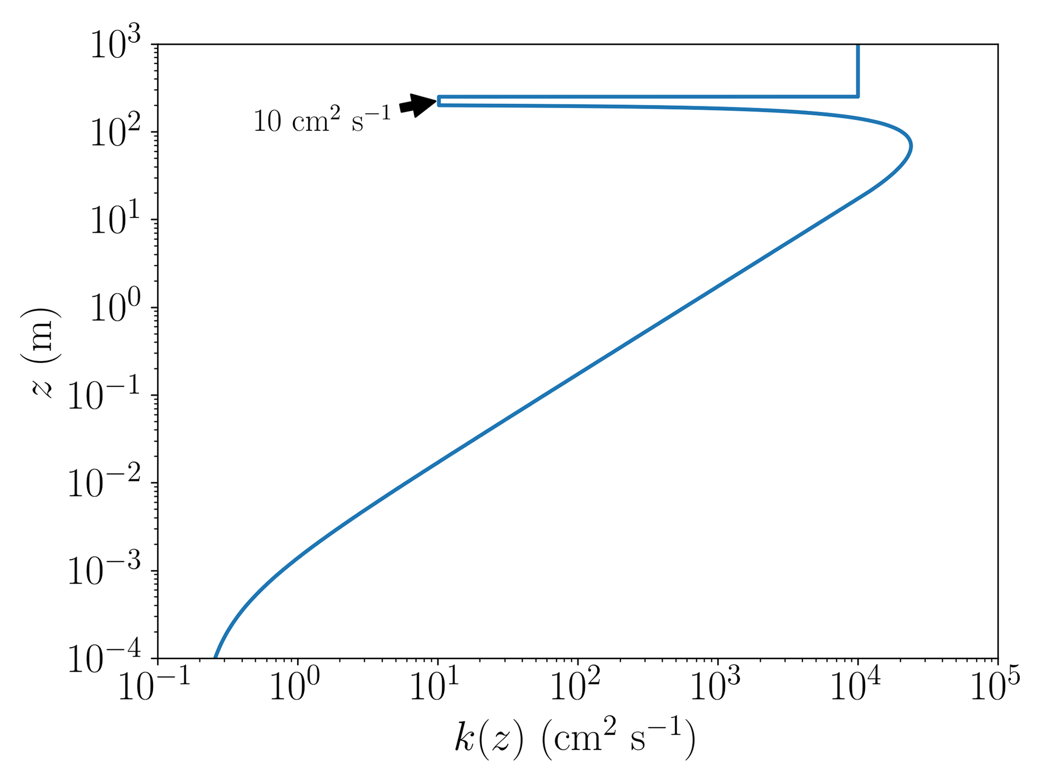
https://www.atmos-chem-phys.net/19/10161/2019/acp-19-10161-2019-f01

Figure 1The turbulent diffusion coefficient k(z) as a function of altitude z for a boundary layer height of 200 m, a wind speed of 5 m s⁻¹, k_f=1 m² s⁻¹, and the inversion layer thickness of 50 m.

Download

The profile of the turbulent diffusivities was chosen to be constant in the present paper. A gradually changing k profile, either by prescribing a time dependence or using real measurements, could force additional oscillations to occur, similar to the recurrence found by Cao et al. (2016), potentially hiding the influence of the chemistry on the oscillations.

2.1.2 Chemical reaction mechanism

The chemical reaction mechanism is based on the bromine/nitrogen/chlorine mechanism of Cao et al. (2014) with a few modifications to the gas-phase mechanism and more complex aerosol modeling. Both modifications are described below. The resulting mechanism encompasses 50 gas-phase species with 175 gas-phase reactions and 20 aerosol-phase species with 50 aerosol-phase reactions. The full reaction mechanism is described in Tables A1–A5 of Appendix A.

For simplicity, the gas-phase concentration of NO_y is assumed to be a conserved quantity in the model. In reality, this is only partly true, since HNO₃ tends to dissolve quickly in aerosols and can become inert, acting as a strong sink. This sink may be compensated by the emissions of NO_x from the snow, which was discussed in the introduction, or by advection of NO_x. The modeling of these processes would add more uncertainties since the emissions and depositions of the various reactive nitrogen species need to be parameterized. Also, in order to correctly model the deposition of HNO₃, detailed aerosol chemistry is needed, which would increase the simulation time. Therefore, gas-phase NO_y is assumed to be conserved in the present model; i.e., no emission and deposition of NO_y and heterogenous reactions involving NO_y are formulated to conserve gas-phase NO_y.

2.1.3 Treatment of the aerosols

The aerosols are modeled as described by Sander (1999) and they are assumed to be liquid. A monodisperse aerosol with a radius r=1 µm is assumed. The pH value is fixed to 5. Simulations found little pH dependence of the oscillation periods for pH values below 7. The aerosols are assumed not to undergo any dynamics except for turbulent diffusion, and the aerosol volume fraction in air is fixed at a value of $ϕ = 10^{- 11}$ m $_{aq}^{3}$ m $_{air}^{- 3}$ . Dry and wet depositions of aerosols as well as productions and emissions of aerosols are neglected. Exploratory simulations show that adding an aerosol deposition velocity in the range of 0.01–0.1 cm s⁻¹ (Wu et al., 2018) increases the oscillation period by 10 %–40 % and decreases the bromide concentration during the build-up phases by approximately 10 %–30 %. However, if a sink for aerosol is introduced, sources for aerosols such as frost flowers or blowing snow should also be implemented. The produced/emitted aerosols are likely to have non-zero bromide content, providing a source for bromine species and potentially countering the effects of the dry and wet deposition. Therefore, for simplicity and in order to avoid the uncertainties in the production and emission mechanisms of aerosols, both sources and sinks of aerosols are neglected. The aqueous reaction constants, acid/base equilibria, mass accommodation coefficients, and Henry's law constants are taken from the box model CAABA/MECCA, version 3.8l (Sander et al., 2011), and they are summarized as follows.

The transfer rate for a gas species is given by

\begin{matrix} (7) & {(\frac{d c_{i, j, g}}{d t})}_{transfer} = k_{t} (ϕ c_{i, j, g} - \frac{c_{i, j, a}}{H_{i} (T)}), \end{matrix}

with the species- and temperature-dependent non-dimensional Henry's law constants H_i(T); cf. Eq. (12). The gas and the aerosol concentrations $c_{i, j, g}$ and $c_{i, j, a}$ , respectively, are in molec. cm⁻³. The transfer coefficient k_t is calculated as

\begin{matrix} (8) & k_{t} = \frac{k_{in}}{ϕ} = \frac{1}{ϕ} {(k_{diff}^{- 1} + k_{coll}^{- 1})}^{- 1} . \end{matrix}

The diffusion limit for gas–aerosol mass transfer k_diff is

\begin{matrix} (9) & k_{diff} = \frac{v_{th} λ ϕ}{r^{2}} = \frac{v_{th} λ A}{3 r}, \end{matrix}

where $λ = 2.28 \times 10^{- 5} \frac{T}{p}$ Pa m K⁻¹ (Pruppacher et al., 1998) is the mean free path with pressure p. In Eq. (9), use of

\begin{matrix} (10) & r = \frac{3 ϕ}{A} \end{matrix}

has been made, including the assumption of a monodisperse aerosol with radius r, the aerosol volume fraction ϕ, and aerosol surface area concentration A. The collision term k_coll (cf. Eq. 8) for the gas–aerosol mass transfer is

\begin{matrix} (11) & k_{coll} = \frac{3 v_{th} α_{i} ϕ}{4 r} = \frac{α_{i} v_{th} A}{4} . \end{matrix}

Here, α_i is the species-dependent mass accommodation coefficient.

The temperature dependence of Henry's law constants of species i is calculated by

\begin{matrix} (12) & H_{i} (T) = H_{i} (T_{0}) \frac{T}{T_{0}} \exp [T_{H_{i}} (\frac{1}{T} - \frac{1}{T_{0}})], \end{matrix}

where $T_{H_{i}} = - Δ_{sol} H / R$ is the enthalpy of dissolution divided by the universal gas constant R, and the mass accommodation coefficients are obtained from

\begin{matrix} (13) & \begin{aligned} α_{i} (T) = \\ {\{1 + (1 / α (T_{0}) - 1) \exp [- T_{α_{i}} (\frac{1}{T} - \frac{1}{T_{0}})]\}}^{- 1}, \end{aligned} \end{matrix}

where T₀=298.15 K. The values for Henry's law constants and the mass accommodation coefficients are given in Table A3. The transfer rate for the corresponding aerosol species from the aerosol phase to the gas phase has the opposite sign.

2.2 Numerical aspects of the model

2.2.1 The numerical grid

A sketch of the numerical grid is displayed in Fig. 2. The computational domain extends 1000 m in the vertical direction and the number of exemplary grid cells is M=32. Different numerical grid resolutions were used to assure grid independence of the numerical solution of the equations; see discussion in the results section.

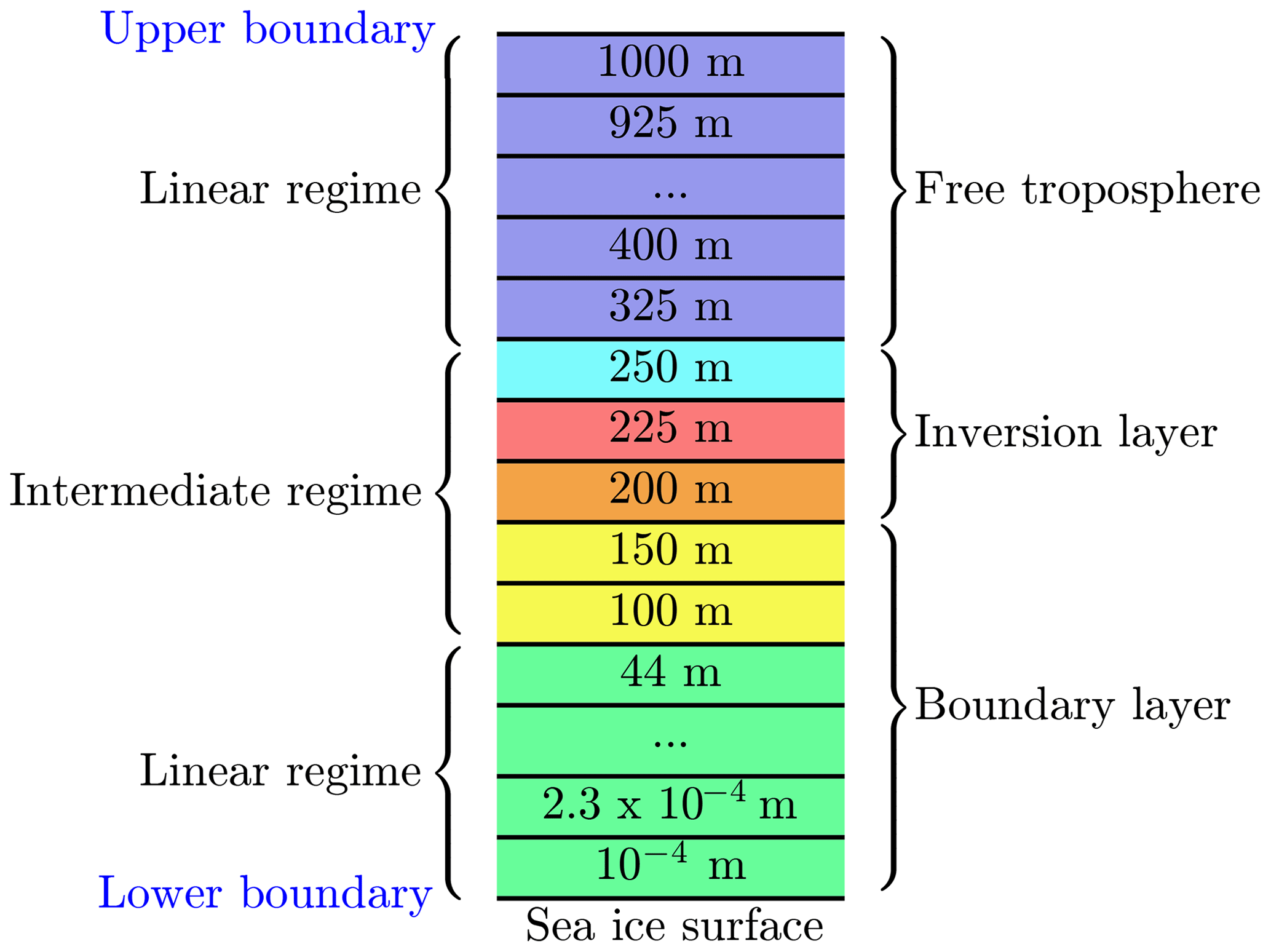
https://www.atmos-chem-phys.net/19/10161/2019/acp-19-10161-2019-f02

Figure 2One-dimensional grid. Numbers are at the center of every numerical grid cell. The red grid cell resides inside the inversion layer. The grid cells at 200 and 250 m are centered at the interface of the inversion layer.

Download

The lowest grid cell at the surface is $z_{1} = 10^{- 4}$ m. The lowest $M / 2 + 1$ grid cells are distributed logarithmically up to 100 m of the computational domain; cf. Fig. 3. In an intermediate regime, it is assured that at least one grid cell resides inside the inversion layer and that there are grid cells on the borders of the inversion layer to ensure a proper resolution the inversion layer. The remaining grid cells are distributed linearly up to the upper boundary at 1000 m. The numerical grid is displayed in Fig. 3, where the first 17 grid cells are logarithmically distributed, followed by five grid cells to resolve the inversion layer. The remaining 10 grid cells are distributed linearly. A black vertical line marks transition from the logarithmic to the linear regime, and the grey area marks the inversion layer.

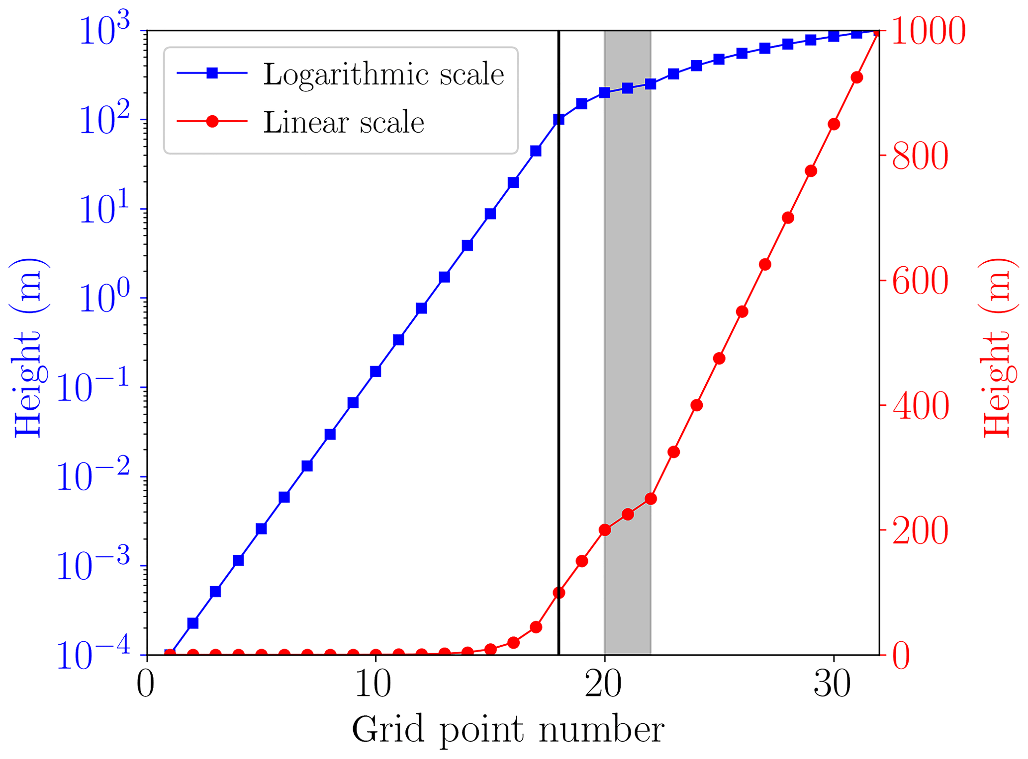
https://www.atmos-chem-phys.net/19/10161/2019/acp-19-10161-2019-f03

Figure 3Numerical grid with M=32 grid cells (cf. Fig. 2) plotted on a logarithmic scale (squares) and a linear scale (filled circles). The grey area shows the inversion layer.

Download

The choice of switching from the logarithmic to the linear grid at 100 and at 200 m was tested, and the numerical results were not affected. The boundary layer height L is 200 m in the present simulations (cf. Table 1), so that the choice of 100 m for the switch of the numerical grid is chosen in order not to interfere with the height of the boundary layer.

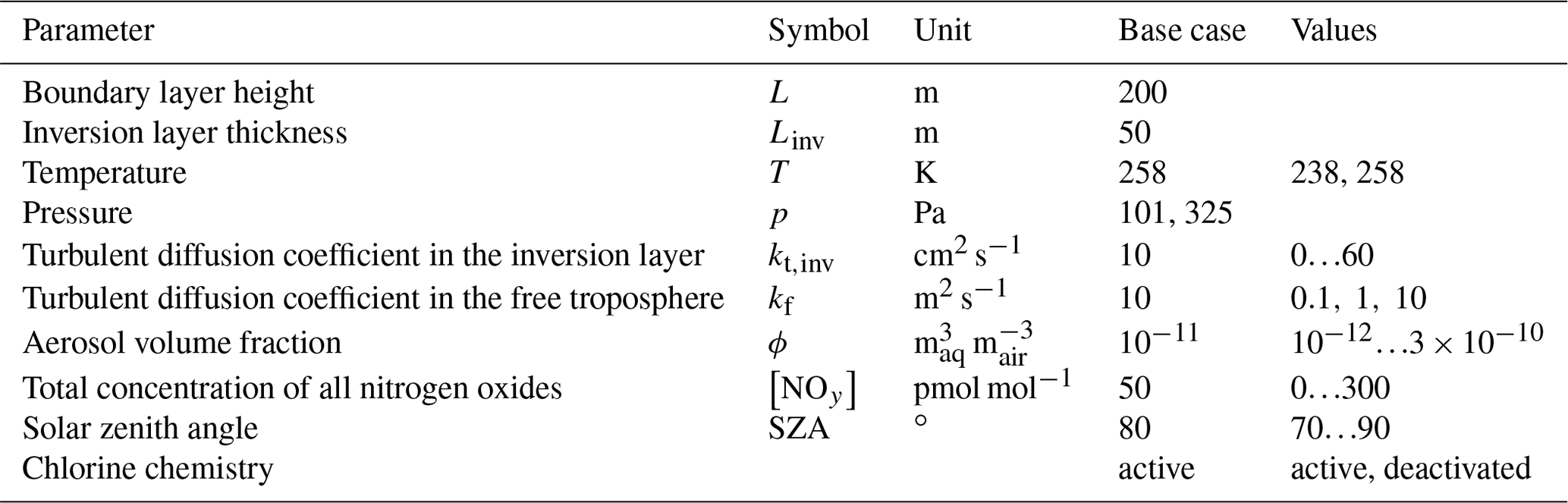
Table 1Parameter definition for the base-case settings and variations used in the parameter study.

Download Print Version | Download XLSX

Most simulations were conducted with 16 grid cells; simulations with 32, 48, and 64 grid cells were also performed to assure grid independence of the results. In Sect. 3.1.1, it is shown that 16 grid cells are sufficient to calculate the oscillation periods with errors smaller than one percent. In total, several hundred simulations for 200 real-time days were conducted in order to study the model parameters (see Table 1), so that the small grid size is convenient to minimize the total runtime of the simulations.

2.2.2 The numerical solver

In order to study the oscillation of ODEs for different parameter settings, the typical real time of about 20 d that was used by Cao et al. (2016) is extended to 200 d in the present study. Scanning the parameter space shown in Table 1 requires hundreds of simulations, so that at first, an optimization of the KINAL-T code (Cao et al., 2016) was conducted.

Cao et al. (2016) decoupled the diffusion terms, the chemical reactions were solved in an implicit way using the Rosenbrock 4 solver (Gottwald and Wanner, 1981), and diffusion was treated in an explicit way. The heterogenous reactions were solved as part of the chemistry equations.

This procedure has some disadvantages. Since the grid is logarithmic for z<100 m, the cell size h_j is h_j∝z in that regime. The diffusion timescale $t_{d} = h_{j}^{2} / k (z) \propto z$ becomes very small for small z, which limits the time steps to the order of milliseconds if an explicit solver is chosen. Also, the heterogenous reactions on the ice surface destroy all HOBr in the lowest cell in some tens to hundreds of microseconds, depending on the size of the grid cells, so that the heterogenous reactions have to be solved as part of the diffusion equations in order to allow mixing of upper layers into the lowest cell during a single time step. Even then, however, time steps smaller than seconds are needed due to the strong coupling of the diffusion and the chemical reactions caused by the heterogenous reactions if the equations are solved completely decoupled. Thus, in the present code, the diffusion equations and the chemical reactions are solved fully coupled with the implicit, A-stable Rosenbrock 4 solver, resulting in a quite large Jacobian matrix of dimension $n = N \times M$ , i.e., the product of the number of species, N, and grid cells, M. The time steps are chosen adaptively, where most time steps are of the order of minutes.

2.3 Base parameters

The base parameter settings as well as the range in which they are varied are shown in Table 1. The values for the temperature T, pressure p, boundary layer height L, aerosol volume fraction ϕ, and solar zenith angle are chosen following Cao et al. (2016).

An inversion layer thickness of L_inv=50 m is chosen. Palo et al. (2017) found values ranging from 20 to 1000 m with a mean of 337 m. In the study of Neff et al. (2008), a shallow boundary layer with L≈165 m and an inversion layer thickness of L_inv≈70 m were found. In the present study, it was found that a larger inversion layer thickness L_inv can be compensated (i.e., leads to a similar behavior in the boundary layer) by choosing a correspondingly larger turbulent diffusion coefficient k_t,inv, with a nearly linear relationship $k_{t, inv} \sim L_{inv}^{1.2}$ . The base parameter settings for the diffusion coefficient in the inversion layer has been determined by searching for the oscillating solutions of the numerical simulations.

The dependence of the oscillation period on [NO_y] was investigated for two different temperatures (258 and 238 K) and with the chlorine mechanism turned on and off. The diffusion coefficients in the free troposphere k_f were varied along with k_t,inv. For sake of simplicity, the solar zenith angle (SZA) was assumed to be constant during a simulation. The base setting of a constant 80^∘ corresponds to the conditions at the North Pole in mid-April.

2.4 Initial and boundary conditions

2.4.1 Initial conditions

The initial species concentrations are shown in Table 2. Initial concentrations of organic species are chosen to be consistent with the study of Hov et al. (1989). Nitrogen-containing species concentrations are varied as shown in Table 2. Emissions of nitrogen from the snow are not considered; instead, NO_y is a conserved quantity in the model. Initial concentrations of bromine are zero in both the free troposphere and in the inversion layer. Starting with non-zero gas-phase bromine concentrations means that the initialization of the bromine explosion is not simulated; the simulation starts during the build-up stage of the bromine explosion.

Table 2Initial trace-gas concentrations.

Download Print Version | Download XLSX

2.4.2 Boundary conditions and heterogenous reactions at the ice surface

The upper boundary of the calculation domain at 1000 m is a Dirichlet boundary where all species concentrations are set to the initial concentrations given in Table 2. The presumed large diffusion coefficient of 10 m² s⁻¹ ensures that the free troposphere is nudged to the initial concentrations on a timescale of hours.

For the boundary at the ice surface, zero flux is assumed. The exchange with the snow/ice surface is modeled via the heterogenous reactions listed in Appendix A in Table A5. An example of the general treatment of a representative heterogenous reaction is

\begin{matrix} (R24) & HOBr + H^{+} + {Br}^{-} \overset{aq}{\to} {Br}_{2} + H_{2} O, \end{matrix}

which is represented as a dry deposition reaction that occurs only in the lowest computational cell. The ice/snowpack itself is not modeled; instead, it is assumed that the salt content is infinite, so heterogenous reactions on the ice surface are effectively treated as

\begin{matrix} (R25) & HOBr \to {Br}_{2} . \end{matrix}

The first-order reaction constants are parameterized by

\begin{matrix} (14) & k = \frac{v_{d}}{h_{1}}, \end{matrix}

where the thickness of the lowest layer is h₁ (cf. Eq. 3), and the dry deposition velocity is v_d. The dry deposition velocity is modeled following the work of Seinfeld and Pandis (2006) as the inverse of the sum of three resistances (R_a, R_b, and R_c):

\begin{matrix} (15) & v_{d} = \frac{1}{R_{a} + R_{b} + R_{c}}, \end{matrix}

described as follows. The values of the resistances are calculated following the work of Huff and Abbatt (2000, 2002). First, the gas is transported from the center of the lowest grid cell z₁ to the top of the interfacial layer at the surface roughness length z₀ by turbulent diffusion, which leads to the aerodynamic resistance:

\begin{matrix} (16) & \begin{aligned} R_{a} & = \int_{z_{0}}^{z_{1}} {(K (z) + D)}^{- 1} d z = \int_{z_{0}}^{L_{1}} {(κ u_{*} z + D)}^{- 1} d z \\ = \ln (\frac{κ u_{*} z_{1} + D}{κ u_{*} z_{0} + D}) / (κ u_{*}) . \end{aligned} \end{matrix}

Then, the gas must be transported through the interfacial layer via molecular diffusion, resulting in the quasi-laminar resistance:

\begin{matrix} (17) & R_{b} = z_{0} / D . \end{matrix}

Finally, the surface resistance is estimated by

\begin{matrix} (18) & R_{c} = 4 / (v_{th} γ), \end{matrix}

with the thermal velocity $v_{th} = \sqrt{8 R T / (π M_{i})}$ . M_i is the molar mass of the gas species undergoing the heterogenous reaction and R is the universal gas constant. For the range of γ in the present study (see Table A5), the aerodynamic resistance is the largest out of the three resistances. For HOBr, Eqs. (16)–(18) result in R_a=0.039 s cm⁻¹, R_b=0.005 s cm⁻¹, and R_c=0.003 s cm⁻¹. Due to the small size of the lowest grid cell, the heterogenous reactions are very fast and their speed is actually limited by the turbulent diffusion of the depositing species from the upper grid cells to the lowest grid cell. The dry depositions of HCl and HBr provide sinks that prevent halogen concentrations from increasing infinitely.

3 Results and discussion

In this section, the mechanism of oscillations of ozone depletion events as well as their possible termination are investigated. First, the reasons for oscillation to occur are discussed and the oscillation period is defined. Second, a closed system with aerosols as the only surface for the recycling of bromine is investigated. Moreover, a comparison to an earlier study (Evans et al., 2003) is presented. Finally, parameter studies are performed on the base parameters presented in Table 1 in order to investigate the variation of the oscillation period.

3.1 Oscillation and termination of ODEs

This section concerns the study of oscillation and termination of ODEs.

3.1.1 Oscillation of ODEs

The oscillation period of an ODE is defined as the average time difference of two consecutive ozone maxima. An ozone maximum is only accepted if the difference in mixing ratio with the preceding ozone minimum is at least 2 nmol mol⁻¹, which is used as a threshold value to distinguish between oscillations and noise.

Figure 4 shows the oscillation of ODEs for the base setting of the present model (cf. Table 1) for 16, 32, 48, and 64 grid cells. The differences between the different grid sizes are small, the average oscillation period varies by less than 1 %, and thus 16 grid cells are sufficient to properly represent the major features of the ODEs and their oscillation.

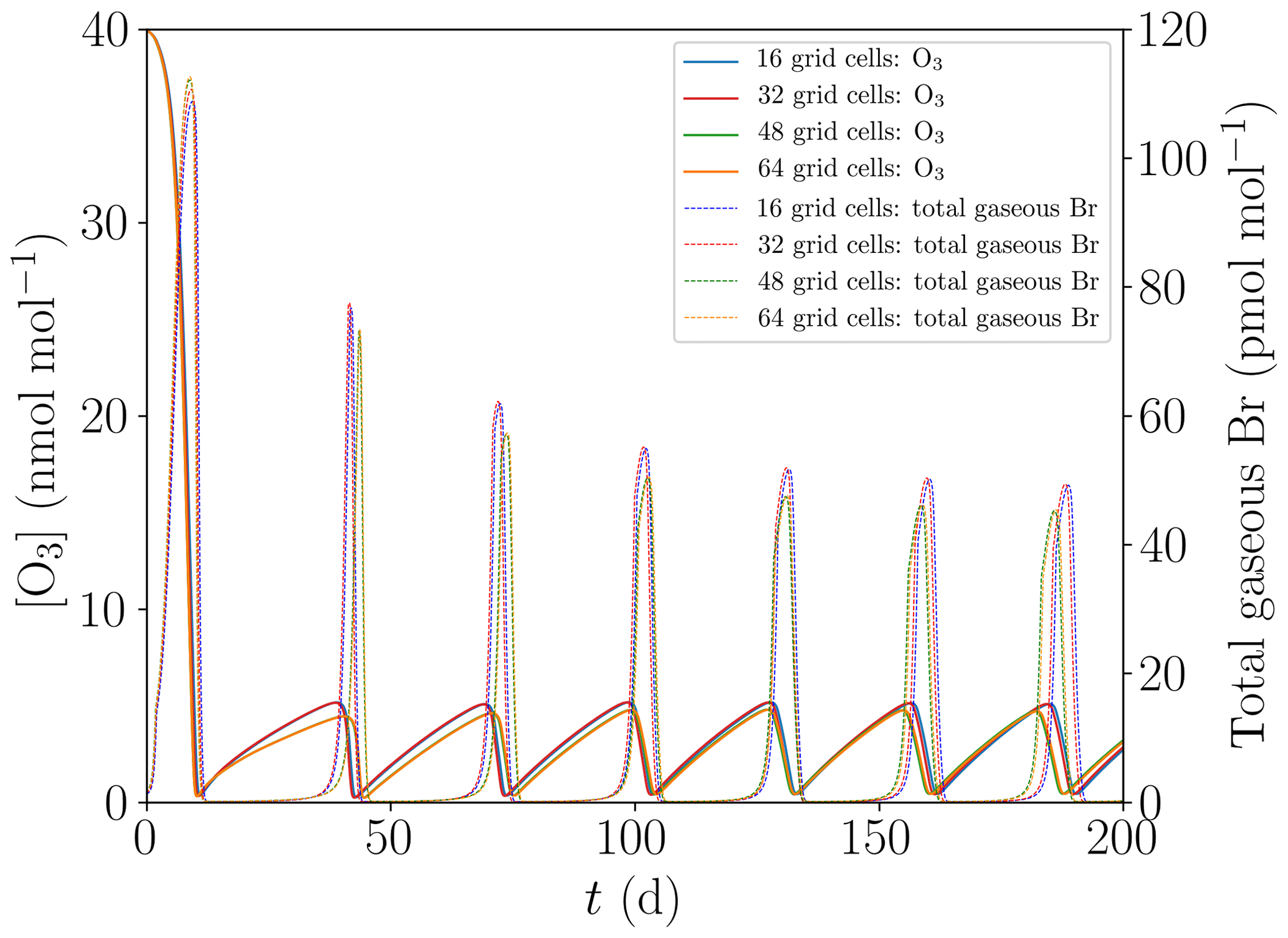
https://www.atmos-chem-phys.net/19/10161/2019/acp-19-10161-2019-f04

Figure 4Evolution of O₃ and total gaseous bromine mixing ratios for four different numbers of grid cells of M=16, 32, 48, and 64.

Download

Oscillation of ODEs may be explained as follows. After the occurrence of an ODE, there is not enough ozone left to sustain the BrO concentration through Reaction (R1), causing bromine to be converted into HBr, which deposits onto the ice/snow surface or onto aerosols and then turns into bromide; cf. Reaction (R12). The now-inactive bromide needs to undergo another bromine explosion (see Reaction R9) in order to become reactive again, which does not occur in the absence of ozone. This allows the ozone in the boundary layer to replenish via the photolysis of NO₂ or by diffusion from the free troposphere through the inversion layer. Once the ozone mixing ratio is large enough, α, defined in Eq. (1), becomes larger than unity, allowing for another bromine explosion. Ozone and reactive bromine now replenish simultaneously where the formation of reactive bromine is becoming faster, increasing the ozone mixing ratio. Once the BrO mixing ratio has reached approximately 10 pmol mol⁻¹, the ozone destruction by bromine becomes larger than the ozone regeneration. Then, another ODE occurs and the cycle repeats. Another sink of bromine in the model is the diffusion of part of the bromine species through the inversion layer, since bromine may leave the computational domain through the upper boundary, where the Dirichlet boundary conditions enforce the bromine concentrations to zero.

However, oscillations do not occur for all parameter settings as can be seen in Fig. 5, where k_t,inv is increased from 10 to 50 cm² s⁻¹. For $k_{t, inv} = 50$ cm² s⁻¹, after the initial ODE and an oscillation with a reduced value of [O₃], no further oscillation occurs. Instead, the reactive bromine and ozone establish a chemical equilibrium, and no further oscillation is observed; i.e., it terminates. The termination of an oscillation will be further discussed next.

https://www.atmos-chem-phys.net/19/10161/2019/acp-19-10161-2019-f05

Figure 5Evolution of O₃ and total gaseous bromine mixing ratios for $k_{t, inv} = 10$ and 50 cm² s⁻¹.

Download

3.1.2 Termination of ODE oscillations

In order to study the termination of ODE oscillations, the initial concentration of [NO_y] is reduced to zero compared to the base case; cf. Table 1. Moreover, the turbulent diffusion coefficient in the inversion layer is increased from the base parameter of 10 cm² s⁻¹, displayed in Fig. 6a, to 20 cm² s⁻¹, shown in Fig. 6b.

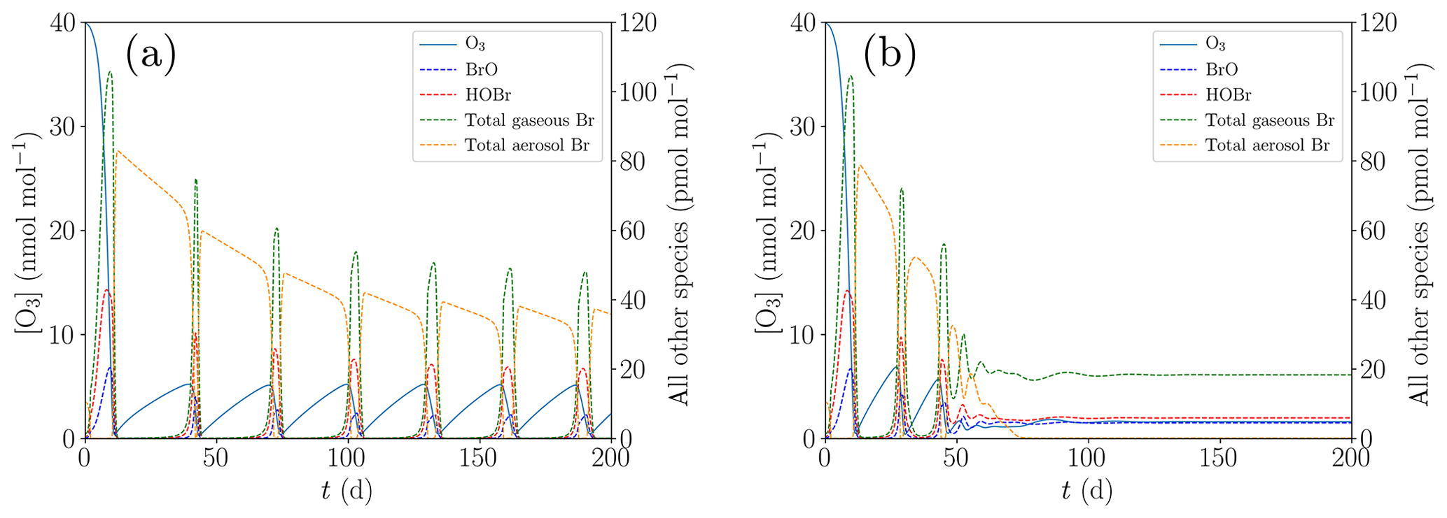
https://www.atmos-chem-phys.net/19/10161/2019/acp-19-10161-2019-f06

Figure 6Oscillation and termination of ODEs for different values of k_t,inv. (a) $k_{t, inv} = 10$ cm² s⁻¹, (b) $k_{t, inv} = 20$ cm² s⁻¹.

Download

If the ozone recovery rate during an ODE is too large compared to the amount of reactive bromine left for α<1 in Eq. (1), the remaining bromine is not sufficient to fully destroy the ozone, leading to shorter oscillation periods and lower levels of ozone peak concentrations as seen in Fig. 6b: bromine levels drop until ozone can regenerate, the regeneration of ozone reactivates a part of the inactive bromine, which in turn depletes ozone until the ozone and the bromine concentrations achieve an equilibrium, and thus only two oscillations occur.

The termination may occur directly after the initial ODE as shown in Fig. 5 or after a few oscillations as a dampened oscillation; see Fig. 6b. The initial ODE typically releases the largest amount of bromine because the initial ozone mixing ratio of 40 nmol mol⁻¹ is much larger than the 10 nmol mol⁻¹ mixing ratio of the oscillations. The total amount of bromine in boundary layer tends to drop after the initial ODE, mostly due to the dry deposition of HBr and to a lesser extent due to diffusion of bromine into the free troposphere.

This reduction in the bromine is the main dampening process. The smaller bromine mixing ratio may not be sufficient to destroy the remaining ozone once α<1 and can thus result in a termination at a later oscillation instead of the termination after the first ODE.

Both a large ozone regeneration rate and a higher Br release efficiency reduce the drop in the total bromine mixing ratio in the gas and aerosol phases that occur between successive oscillations. If the bromine release or ozone regeneration rate are sufficiently large, the bromine mixing ratio may increase for successive oscillations, as shown in Fig. 7. The additional ozone production due to an increased initial NO_y mixing ratio shortens the oscillation period and therefore limits the bromine losses occurring between successive bromine explosions.

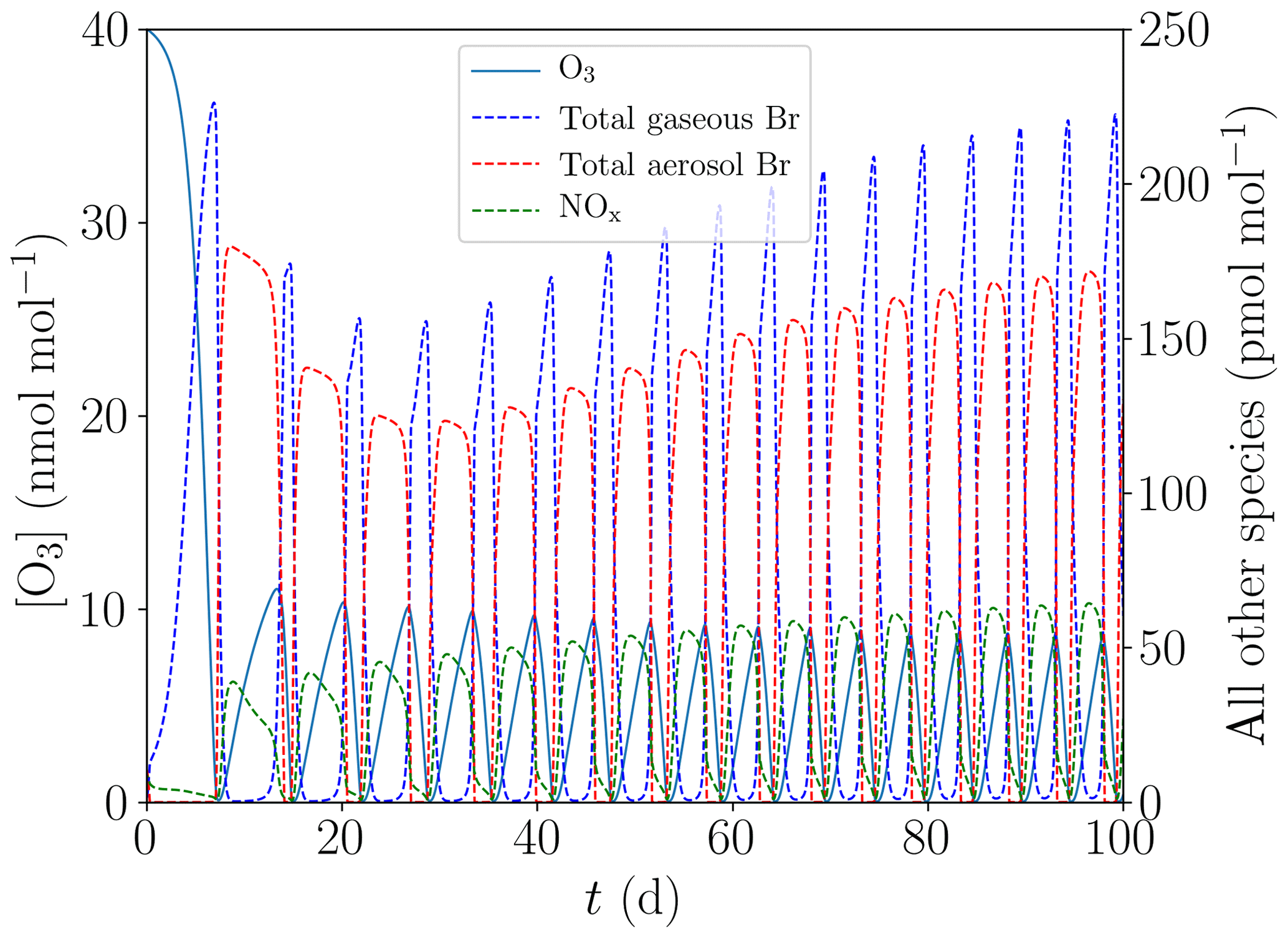
https://www.atmos-chem-phys.net/19/10161/2019/acp-19-10161-2019-f07

Figure 7Evolution of O₃, NO_x, and total gaseous and aerosol bromine mixing ratios for the base case with [NO_y]=150 pmol mol⁻¹.

Download

Termination may not occur at all during 200 d. Typically, the oscillation period becomes constant after the first few oscillations. The first oscillations are affected by the initial value of 40 nmol mol⁻¹ for the ozone concentration. The fate of most of the bromine after an ODE is to be stored in aerosols as bromide. While the initial bromine explosion is mostly driven by heterogenous reactions on the ice/snow surface, the bromine explosions of the oscillations are driven by heterogenous reactions on the aerosols, which now hold a significant amount of bromide. After a few oscillations, the bromine deposited on the ice surface or diffused to the free troposphere between each oscillation becomes equal to the bromine released from the ice surface during each oscillation, resulting in a constant oscillation period thereafter.

In order to observe fast oscillations, an O₃ recovery rate of more than 1 nmol mol⁻¹ per day is required. However, as noted above, for an ODE to terminate properly, the O₃ recovery rate during the termination of an ODE may not be too large. Figures 5 and 6 show a termination due to a sufficiently large k_t,inv.

The effect of a strong inversion layer as well as the ozone formation via nitrogen oxides on ODEs will be studied in Sect. 3.4. The next subsection concerns different ways of initialization of ODEs.

3.2 Initialization of an ODE with only aerosols

So far, the ODEs were initiated through the assumption of a fixed value of 0.3 pmol mol⁻¹ Br_x inside the boundary layer (cf. Table 2). In the present subsection, another mechanism for the initiation is studied, where aerosols are used to initiate the ODEs. Five assumptions are changed with regard to the base case:

The concentration of Br⁻ was set to 0.8 mol L⁻¹, corresponding to a mixing ratio of 160 pmol mol⁻¹ in the gas phase, which is different from the base setting of 0.05 mol L⁻¹ (equivalent to 10 pmol mol⁻¹) shown in Table 2.
The turbulent diffusion coefficient in the inversion layer is set to zero.
The initial concentration of gas-phase bromine is set to zero.
All heterogenous reactions on the ice/snow surface are turned off.
The [NO_y] is increased from 50 to 100 pmol mol⁻¹.

The large concentration of Br⁻ could be caused by a blowing snow event. In this simulation, the main source of the first reactive bromine is via the heterogenous reaction of ozone; see Reaction (R19).

As a result of the different settings, the total bromine concentration is conserved during the simulation. Furthermore, the boundary layer is a closed system for this simulation. The results are shown in Fig. 8.

https://www.atmos-chem-phys.net/19/10161/2019/acp-19-10161-2019-f08

Figure 8Simulation neglecting the snowpack and the exchange between the boundary and the inversion layers.

Download

After 1 h, already 0.1 pmol mol⁻¹ of reactive bromine is reactivated, which is sufficient for the bromine explosion on aerosols to become the dominant reactivation mechanism. Also, N₂O₅ can activate the first bromine by producing BrNO₂. Reactive chlorine can also activate the first bromine, however, more slowly. Overall, 0.3 pmol mol⁻¹ of reactive chlorine takes several days to produce an initial seed of 0.1 pmol mol⁻¹ reactive bromine. Only in the first time steps, bromine is reactivated by the very slow release of Br via HOCl; see Reaction (R18).

After that, a regular bromine explosion occurs, albeit restarting from very low concentrations of 10⁻⁴ pmol mol⁻¹ [Br_x]. The initialization via reactivation of bromine on aerosols is much faster than reactivation via the ice surface, since the multiphase reactions involving aerosols are not diffusion limited. All other episodes start from about 30 pmol mol⁻¹ of bromide in the aerosol phase, which is why they have longer induction stages of about 10 d compared to a few hours for this simulation.

It is of particular interest that oscillations occur without any external sources and sinks, such as dry depositions, emissions, or heterogenous reactions on the ice/snow surface. The density of each chemical element in the gas plus aerosol phase is conserved in this simulation, with hydrogen being the only exception due to the constant pH value of the aerosols. Due to the second law of thermodynamics, only reaction intermediates may oscillate. As an example, CO₂ is a permanent sink for other organic species in this simulation. It is expected for the oscillations to terminate after a sufficient amount of reactive organics is converted to non-reactive organics.

3.3 Comparison to studies in the literature

The most relevant research in the area of oscillating ODEs was performed by Evans et al. (2003) which is used to validate the present model. Similar to the aerosol-only simulation of the previous subsection, aerosols are the only source and sink for bromine in the system studied by Evans et al. (2003).

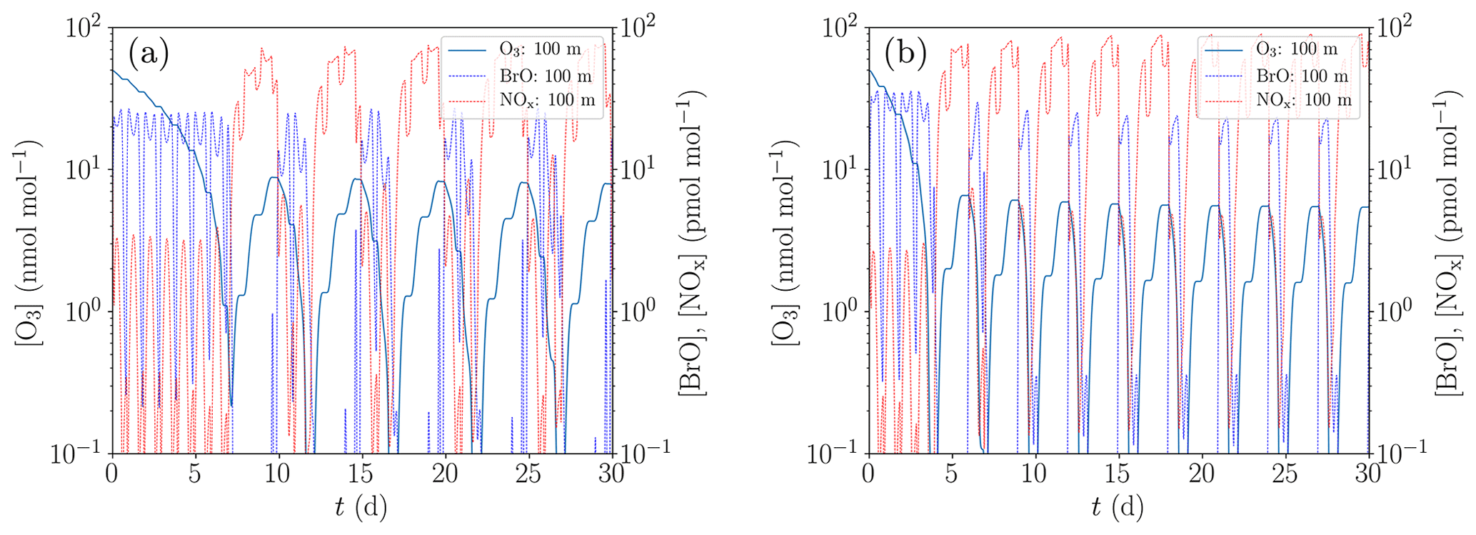
https://www.atmos-chem-phys.net/19/10161/2019/acp-19-10161-2019-f09

Figure 9Simulation of the oscillations of ODEs for the conditions of Evans et al. (2003). (a) Low NO_x emission and initial bromide mixing ratio of 43 pmol mol⁻¹. (b) Increased NO_x emission by 35 % and initial bromide mixing ratio of 60 pmol mol⁻¹.

Download

A comparison between the model of Evans et al. (2003) and the present study is displayed in Fig. 9, where Fig. 9a is for a low NO_x emission and an initial bromide mole fraction of 43 pmol mol⁻¹ and Fig. 9b for elevated NO_x emission by 35 % and an initial bromide mole fraction of 60 pmol mol⁻¹.

Differences in the model and in the conditions are as follows:

The gas–aerosol mass transfer rates used by Evans et al. (2003) are approximately 20 times larger than these in the present work. Evans et al. (2003) employ the parameterization described by Michalowski et al. (2000). In that study, the diffusion-limit term k_diff (Eq. 9), which appears in the gas-to-aerosol transfer constant k_in (Eq. 8) of the present paper, is neglected and only k_coll (Eq. 11) has been considered. However, the values used for k_coll and for k_in are also different. For the species HOBr, for instance, the base parameters in the present study are $k_{coll} = 8.9 \times 10^{- 4}$ s⁻¹ and $k_{in} = 1.2 \times 10^{- 4}$ s⁻¹. Using the values for the oscillating result of Evans et al. (2003) and estimating the aerosol radius via Eq. (10), which results in r=0.3 µm, the corresponding values are $k_{coll} = 2.0 \times 10^{- 3}$ s⁻¹ and $k_{in} = 5.0 \times 10^{- 4}$ s⁻¹. These differences result not only from negligence of the diffusion limit but also from a larger accommodation coefficient (α=0.8 compared to α=0.5) as well as a larger aerosol surface area ( $A = 4.4 \times 10^{- 7}$ cm² cm⁻³ versus $A = 3 \times 10^{- 7}$ cm² cm⁻³).
NO_x and HCHO are emitted from the snowpack as described by Evans et al. (2003). The emission rate is proportional to the photolysis rate of NO₂ with an average emission rate of 1.2×10⁹ molec. cm⁻² s⁻¹ for NO_x and 3.6×10⁸ molec. cm⁻² s⁻¹ for HCHO.
HNO₃ transfer to aerosols is considered and it acts as a sink for NO_y.
All heterogenous reactions and deposition on the ice surface are neglected. However, following Evans et al. (2003), PAN and H₂O₂ undergo dry depositions with velocities of v_d=0.004 cm s⁻¹ and v_d=0.09 cm s⁻¹, respectively.
The SZA is varied daily in the range of 65 to 97^∘ following a cosine profile, which is consistent with a latitude of 73.4^∘ on 15 April 2003.
Initial concentrations and parameters are set to the values described by Evans et al. (2003). In particular, the initial mole fraction of bromide is set to 43 pmol mol⁻¹. In contrast to the study of Evans et al. (2003), the mixing ratio of acetaldehyde CH₃CHO may evolve freely instead of being fixed to 18 pmol mol⁻¹.
Reactions involving the species BrNO₂ are neglected since the species BrNO₂ is not considered by Evans et al. (2003).

The results presented in Fig. 9 show that with an initial bromide mole fraction of 43 pmol mol⁻¹, the oscillation period is approximately 5 d. The chemical reaction mechanism used in the present KINAL-T code predicts larger HBr and HOBr mixing ratios compared to the model employed by Evans et al. (2003), resulting in smaller BrO mixing ratios for the same total bromine mole fraction and thus slower ODEs. Ozone is completely depleted approximately 1 d after the ODE has started, which is more than twice as long as predicted by Evans et al. (2003). Also notably, ozone replenishes to approximately 8.5 nmol mol⁻¹ before the ODE starts, whereas Evans et al. (2003) predict only approximately 4.5 nmol mol⁻¹. This suggests that the bromine regeneration is slower or that less reactive bromine remains after an ODE in the present KINAL-T simulation. After an ODE, reactive bromine mixing ratios drop to approximately 10⁻⁴ pmol mol⁻¹ in the present simulation. The bromine regeneration rate is approximately 1 order of magnitude per day in the present simulation. This means that if the bromine regeneration rate is the same but the reactive bromine mixing ratio obtained by Evans et al. (2003) drops to 10⁻² pmol mol⁻¹ after an ODE, which might explain the difference.

Neglecting the role of BrNO₂ chemistry has been found to be of particular importance for finding oscillations of ODEs, since otherwise BrNO₂ acts as a sink for both bromine and NO_x. If BrNO₂ chemistry is considered, similar structures to those seen in Sect. 3.4.2 for large NO_y mixing ratios are found, where the large NO_y concentrations cause a termination of the oscillations.

Another issue of importance is the larger gas–aerosol mass transfer constants used by Evans et al. (2003) compared to the present study. The gas-to-aerosol transfer constants used by Evans et al. (2003) are of the order of 10⁻³ s⁻¹ compared to 10⁻⁴ s⁻¹ for the base case. In the present study, the latter value has been adjusted to that used by Evans et al. (2003) in order to match their results. These increased coefficients allow for a quick recycling of HOBr, HBr, and BrONO₂. With smaller gas–aerosol mass transfer constants, the bromine regeneration after an ODE slows down and, more importantly, a larger initial bromide mixing ratio (more than 100 pmol mol⁻¹) is necessary to achieve BrO mixing ratios of at least 20 pmol mol⁻¹ during an ODE. At an initial bromide mixing ratio of 43 pmol mol⁻¹, the ozone depletion occurs on a timescale of weeks with the slower gas–aerosol mass transfer constant.

As discussed above, Michalowski et al. (2000) and Evans et al. (2003) ignored the diffusion limit. Staebler et al. (1994) measured a maximum value of r=0.1 µm in the aerosol size distribution at Alert, and therefore Evans et al. (2003) assumed that the diffusion correction may be neglected for this small value of aerosol size. However, even at r=0.1 µm, the HOBr transfer constants are calculated to decrease by a factor of 2 in the present study, which provides the motivation to consider its relevance in the present study. The aerosol transfer, however, is driven by the aerosol surface, which motivates the use of the aerosol surface distribution instead of the aerosol size distribution. This causes another shift towards larger aerosol sizes with an increased effect on the diffusion limit.

In order to reproduce the oscillation period of 3 d predicted by Evans et al. (2003), a second simulation with an increased initial bromide mixing ratio of 60 pmol mol⁻¹ and increased NO_x emissions by 35 % was conducted; cf. Fig. 9b. The main effect of the increased initial bromide mixing ratio alone is a decrease of the duration of the ODEs from 1 d to somewhat less than half a day and as a consequence, the oscillation period reduces by about half a day. The increased initial bromide mixing ratio, however, barely affects the bromine regeneration speed, since it is limited by the low mixing ratio of reactive gas-phase bromine (less than 10⁻⁴ pmol mol⁻¹) after the termination of the ODEs and not by the aerosol-phase bromide concentration. The increased NO_x emissions affect both the ozone regeneration and the bromine regeneration. The latter is not only increased by the larger ozone regeneration speed but also by the bromine explosion mechanism involving BrONO₂. More BrO reacts to BrONO₂, which quickly recycles bromide due to the large gas–aerosol mass transfer coefficients. Consequently, the ODEs start at an ozone mixing ratio of approximately 6 nmol mol⁻¹ compared to the 8.5 nmol mol⁻¹ for the previously used emission rate. Thus, the increased emissions reduce the oscillation period by about 1.5 d, resulting in the shorter oscillation period of ODEs found by Evans et al. (2003). The differences between the numerical results by Evans et al. (2003) and the present study are most likely due to the different chemical reaction mechanisms. Even though Evans et al. (2003) used the reaction constants provided by the same group as the present study, the knowledge about chemical reaction constants has greatly improved in the last decade (Atkinson et al., 2007). Moreover, it should be noted that Evans et al. (2003) used a box model, whereas in the present study, the one-dimensional KINAL-T code with a more advanced model for the heterogenous reactions and the aerosol treatment is used.

3.4 Study of model parameters influencing the oscillation period

This subsection concerns the variation of some environmental parameters that affect the oscillation of ODEs: the strength of the inversion layer, the turbulent diffusion in the free troposphere, the NO_y mixing ratio, the aerosol volume fraction as well as the solar zenith angle on the oscillation period of the ODEs; cf. Table 1. The variation of the NO_y mixing ratio is investigated for T=258 K (base setting) and T=238 K, as well as simulations where the chlorine mechanism is used (base setting) or neglected.

In the following, three properties of the oscillations of ODEs will be considered: the average oscillation period, i.e., the time difference between two ozone maxima, the number of oscillations, and the average maximum of the ozone mixing ratio; these characteristics are evaluated for a real time of 200 d.

3.4.1 Strength of the inversion layer

Diffusion from aloft is one of the two mechanisms that replenishes the ozone in the model. Since the thickness of the inversion layer is fixed (see Table 1), the turbulent diffusion constant k_t,inv is the most important parameter controlling the strength of this replenishment. The turbulent diffusion constant in the free troposphere, k_f, also plays an important role.

https://www.atmos-chem-phys.net/19/10161/2019/acp-19-10161-2019-f10

Figure 10Dependence of the oscillation characteristics on the variations of k_t,inv and k_f (a–c), and the variation of the mixing ratios of O₃ and Br at two different heights (100 and 225 m) for the base settings (d). (a) Average oscillation period during 200 d. (b) Number of oscillations during 200 d. (c) Average maximum mixing ratio of ozone. (d) Profiles of the mixing ratios of O₃ and total gaseous Br.

Download

In order to eliminate the influence of the ozone regeneration by NO₂, the concentration of NO_y is set to zero for evaluation purposes. In Fig. 10, the dependence of the oscillation characteristics on the variations of k_t,inv and k_f is shown (cf. Fig. 10a–c), and the variation of the mixing ratios of O₃ and Br at two different heights (100 and 225 m; Fig. 10d) for the base settings.

The smallest oscillation period of approximately 20 d is found for the turbulent diffusion coefficient of k_f=10⁵ cm² s⁻¹ in the free troposphere and for $k_{t, inv} \approx 40$ cm² s⁻¹. For very small turbulent diffusion coefficients of less than $k_{t, inv} = 6$ cm² s⁻¹, no oscillations occur since the ozone regeneration rate is too slow in the considered time of 200 d.

The oscillation period does not increase linearly with k_t,inv since the ozone mixing ratio in the inversion layer changes with increased diffusion; three processes determine the ozone mixing ratio:

In the inversion layer, ozone is lost by diffusion into the boundary layer.
Ozone is replenished by its diffusion from the free troposphere into the inversion layer.
Bromine is mixed into the inversion layer and lost to the free troposphere, resulting in a partial ODE inside the inversion layer.

Inside the inversion layer, reactive bromine may survive due to the sustained ozone supply from the free troposphere. It turns out that larger diffusion coefficients inside the inversion layer result in increased ozone mixing ratios, converging to approximately 20 nmol mol⁻¹ for k_inv>20 cm² s⁻¹, which is half of the value at the top boundary of the computational domain. This is the reason for the sharp, nonlinear increase in the number of oscillations during 200 d.

For k_inv<14 cm² s⁻¹, the oscillation period decreases strongly, and for larger values of k_inv, termination is initiated. The mixing ratios for O₃ and Br in the first regime, i.e., for k_inv=10 cm² s⁻¹, are displayed in Fig. 10d. After the first ODE, the ozone regeneration due to diffusion is not very much affected by an ongoing ODE since the ozone mixing ratio is only slightly varying inside the inversion layer, severely limiting the ozone regeneration rate without termination.

Since the standard value of k_f=10⁵ cm² s⁻¹ used in the present simulation corresponds to an almost perfectly mixed free troposphere, even larger values do not affect the simulation results. By neglecting horizontal mixing and transport, it is essentially assumed that the air mass in the boundary layer is confined. However, the free troposphere will still have very different wind velocities, so it is reasonable that the air in the free troposphere is exchanged quickly with fresh air even though the boundary layer is confined. A large turbulent diffusion coefficient in the free troposphere ensures a quick exchange of the air with the upper simulation boundary.

The influence of a reduction of k_f to values of 10⁴ and 10³ cm² s⁻¹ is presented in Fig. 10a–c. The value of k_f=10⁴ cm² s⁻¹ still corresponds to nearly perfect mixing inside the free troposphere as can be seen by the negligible differences in the mean oscillation period between k_f=10⁵ cm² s⁻¹ and k_f=10⁴ cm² s⁻¹. All resulting profiles are very similar.

Reducing k_f to 10³ cm² s⁻¹, however, has a large impact, since bromine transported to the free troposphere will stay there for several weeks (as may be estimated from the diffusion timescale) before being transported to the upper boundary. Ozone is also transported much more slowly to the lower layers of the free troposphere, causing the ozone levels to drop to approximately 15 nmol mol⁻¹ at 500 m for $k_{t, inv} = 25$ cm² s⁻¹; ozone levels decrease further with increased values of k_t,inv, converging to 12 nmol mol⁻¹ for k_t,inv exceeding 50 cm² s⁻¹. The ozone mixing ratio in the inversion layer drops to less than 10 nmol mol⁻¹, reducing the ozone recovery rate in the boundary layer and also limiting the maximum levels to which ozone can be recovered.

Oscillations occur only at larger turbulent diffusion coefficients of k_t,inv > 14 cm² s⁻¹, and they terminate for k_t,inv > 50 cm² s⁻¹; see Fig. 10b. In contrast to the larger values k_f, the ozone mixing ratio in the inversion layer decreases with increasing k_t,inv in the present case. Also, the time between two oscillations tends to increase progressively after each oscillation since a larger turbulent diffusion coefficient in the inversion layer causes a greater loss of bromine to the free troposphere, which in turn decreases the speed of the bromine explosion in the boundary layer.

In cases where only two or three maxima occur, i.e., k_inv > 16 cm² s⁻¹, due to the termination of the oscillations, the standard deviation of both the oscillation period and the ozone maxima increase sharply, since the first few oscillations are still affected by the first ODE, and the oscillations before the termination tend to have ozone maxima that are closer to the equilibrium mixing ratio of ozone.

3.4.2 The role of NO_y, T and chlorine

In the present model, NO_y is treated as a conserved quantity. In this subsection, the NO_y mixing ratio is varied as the major parameter influencing NO_x-catalyzed photochemical O₃ formation (see Reaction R20), and its effect on the ODEs is investigated.

https://www.atmos-chem-phys.net/19/10161/2019/acp-19-10161-2019-f11

Figure 11Dependence of the oscillation characteristics on the variations of [NO_y] (a–c). Termination of an ODE: profiles of the mixing ratios of various species for the base settings and for 238 K and [NO_y]=100 pmol mol⁻¹ (d). (a) Average oscillation period during 200 d. (b) Number of oscillations during 200 d. (c) Average maximum mixing ratio of ozone. (d) Profiles of the mixing ratios of O₃ and total gaseous Br.

Download

Figure 11 shows the variation of the oscillation period with NO_y mixing ratios of up to 300 pmol mol⁻¹ for two different temperatures of 258 K (standard value) and the reduced value of 238 K; cf. Fig. 11a. Oscillation periods of less than 5 d are obtained for 258 K. The number of oscillations increases linearly with the NO_y mixing ratio (Fig. 11b), with a y intercept given by the regeneration of ozone purely via diffusion through the inversion layer. At about [NO_y]=200 pmol mol⁻¹ for T=258 K, oscillations tend to terminate. Once the mixing ratio of NO_y is very large, the bromine released during an ODE is not able to completely destroy all NO_x. Thus, even during an ODE, ozone is produced by the NO₂ photolysis, increasing ozone regeneration and making a termination more likely. The non-zero NO_x concentrations also result in more BrNO_x (which is the sum of BrNO₂ and BrONO₂) formation during the termination. BrNO_x then makes up approximately 60 % of the total gas-phase bromine.

Moreover, the chlorine mechanism has been deactivated by setting all chlorine initial concentrations to zero and changing the heterogenous reaction of HOBr to only release Br₂; see Fig. 11a and b. While the presence of chlorine may enhance the ODE by enhanced O₃ destruction through the very fast reaction of BrO with ClO, the bromine explosion is actually slowed down by the presence of chlorine. This is due to the fact that when chlorine is included, part of the heterogenous reactions release BrCl instead of Br₂; thus, the amount of released bromine is reduced. Also, without chlorine, the slower ODE increases the duration of the bromine explosion, which also increases the bromine released, resulting overall in faster oscillations, since further oscillations contain more bromine in aerosols that can be reactivated. As a side effect, the ozone maximum value is slightly smaller without the chlorine chemistry.

For T=238 K, the oscillation period is smaller compared to T=258 K for small [NO_y], as can be seen in Fig. 11c. However, termination of oscillations starts already at around 70 pmol mol⁻¹ of NO_y instead of at around 200 pmol mol⁻¹ for T=258 K. Figure 11d shows a termination for T=238 K after 80 d. In this temperature region, HNO₄ becomes very stable due to the decay of HNO₄ being nearly 2 orders of magnitude slower (see Reaction 56 in Table A1) and replaces PAN as the most abundant nitrogen species. The shift towards HNO₄ formation reduces the NO₂ concentration, retarding the ozone regeneration.

At the lower temperature, the ODE mechanism becomes more efficient, e.g., the reaction constant in the Br₂-producing BrO self-reaction increases by 33 % (Reaction 5 in Table A1), while many of the HBr-producing reactions, e.g., Reactions (9) and (10) in Table A1, slow down by around 20 %. The total amount of bromine released for the first ODE increases, whereas the amount of bromine released for the oscillations decreases due to the slower ozone regeneration.

The main reason for the earlier termination of the oscillations at T=238 K is a strong shift towards the increased HNO₄ formation. During an ODE, the HNO₄ can be destroyed to directly produce NO₂ by reacting with OH or by decaying through Reactions (56) and (57) in Table A1. PAN, however, is more stable during an ODE at 258 K due to a larger formation of CH₃CO₃ via, e.g., Reaction (34) in Table A1 caused by the larger OH formation during an ODE, consuming NO₂ (Reaction 65) instead of producing it through Reaction (84) or through the photolysis of PAN. The shift from PAN as the most stable species towards HNO₄ for the lower temperature increases the ozone recovery during an ODE. Since a larger ozone recovery during an ODE facilitates chemical equilibrium with the reactive bromine, this results in earlier terminations of the oscillations of ODEs.

3.4.3 The influence of the aerosol density

In order to study the influence of the aerosol characteristics, the standard value of the aerosol volume fraction of 10⁻¹¹ m³ m⁻³ is varied between 10⁻¹² and $3 \times 10^{- 10}$ m³ m⁻³; see Fig. 12. For small aerosol concentrations, the recycling of HBr is too weak for a full ODE to occur since only small bromine concentrations are released before the termination of an ODE. Only a partial ODE and no oscillations take place.

https://www.atmos-chem-phys.net/19/10161/2019/acp-19-10161-2019-f12

Figure 12Oscillation characteristics depending on the aerosol volume fraction after 200 d. (a) Mean oscillation period. (b) Average maximum ozone mixing ratio.

Download

For larger aerosol mixing ratios, the faster bromine recycling reduces the oscillation period; however, the ozone does not regenerate faster. Thus, the ozone maximum decreases so that the oscillations release less bromine, resulting in a larger net bromine loss per oscillation. Also, the reactivation strength of aerosol bromine increases relative to the activation on the ice surface, resulting in a lower bromine release from the ice, also increasing the net bromine loss for each oscillation, which ultimately leads to the termination of the oscillations for aerosol volume fractions larger than about $5.5 \times 10^{- 11}$ m³ m⁻³.

3.4.4 Variation of the solar zenith angle

The mean oscillation period displayed in Fig. 13a hardly changes when the SZA is varied from its standard value of 80^∘ (see Table 1) within the range of 70 and 83^∘. The variations stay within 1 standard deviation. For $SZA > 83^{\circ}$ , the ODEs do no longer occur due to the slow photolysis frequencies. Surprisingly, the oscillation period does not monotonically decrease with increased SZA; instead, there is a minimum at $SZA = 77^{\circ}$ . For a lower SZA, some or even all ODEs are only partial, as Fig. 13b demonstrates for the value of $SZA = 70^{\circ}$ . In particular, the minimum ozone mixing ratio for the six oscillations shown is approximately 10 nmol mol⁻¹ and the ozone depletion restarts at an ozone mixing ratio of about 18 nmol mol⁻¹. For a SZA of 70^∘, the NO₂ mixing ratio decreases to about 5 pmol mol⁻¹ during the ODEs instead of to nearly zero at 80^∘. Also, BrNO_x and PAN are photolyzed faster, increasing the NO_x formation. Only about 80 pmol mol⁻¹ of bromine is released at $SZA = 70^{\circ}$ during the first ODE, which is about two-thirds of the value at 80^∘. Interestingly, gas-phase bromine does not drop to zero for the later oscillations; however, the BrO concentration drops to nearly zero. BrO mixing ratios do not exceed 10 pmol mol⁻¹, which is much lower than the typical mixing ratio of 30–40 pmol mol⁻¹ of numerical simulations with a SZA of 80^∘; this is most likely a result of the increased formation of HO₂.

https://www.atmos-chem-phys.net/19/10161/2019/acp-19-10161-2019-f13

Figure 13(a) Mean oscillation period and number of oscillations versus the solar zenith angle during 200 d. (b) Evolution of the mixing ratios of O₃ and the bromine species for $SZA = 70^{\circ}$ .

Download

Another characteristics are the faster photolysis reactions of BrO and HOBr for lower SZA. For $SZA = 70^{\circ}$ , 80 % of the BrO photolyzes to Br and to O₃, which results in a null cycle. The resulting smaller BrO mixing ratio also decreases the rate of self-recycling, which is part of the ozone-destroying cycle. Overall, 70 % of the HOBr photolyzes to HO and Br, slowing down the bromine explosion substantially and consuming HO₂ in the process. The faster Br₂ photolysis, however, does not further enhance the ozone destruction, since Br₂ is already photolyzed extremely fast even at $SZA = 80^{\circ}$ .

For $SZA = 70^{\circ}$ , the fastest reaction of BrO is with NO, producing NO₂ and Br in the process. NO₂ is photolyzed to ozone, resulting in a net null cycle. For $SZA = 80^{\circ}$ , the BrO self-reaction is stronger than its reaction with NO, favoring a full ODE.

4 Conclusions

In the present study, the one-dimensional KINAL-T model developed by Cao et al. (2016) was extended and optimized in order to study the potential of ODEs to recur. The extension concerns the chemical reaction mechanism as well as the treatment of aerosols and the improvement of the numerical solver. The model was employed to study both the oscillation and the termination of ODEs, and several parameters were varied to investigate their influence on the oscillation period, the maximum ozone mixing ratio, and the number of oscillations of the ODEs. After an ODE, ozone can be replenished by the diffusion of ozone from the free troposphere to the boundary layer and/or by the photolysis of NO₂; it is found that either of these two O₃ sources is sufficient to drive the oscillations. Another result of the present study is that the chemistry of ODEs coupled with the vertical diffusion alone can cause the oscillation of ODEs at the surface even without the existence of horizontal transport.

A strong inversion layer was found to be essential for the oscillation of ODEs since the steady mixing of the ozone back into the boundary layer may provide a sufficiently high ozone level to keep the reactive bromine in the boundary layer at a significant level, which then establishes chemical equilibrium with the remaining ozone.

Without the presence of reactive nitrogen oxides, the system is a chemically heterogenous, diffusion-driven oscillating system, the fastest periods of which were found to be approximately 20 d. Fast replenishment of the air in the free troposphere was found to lead to faster oscillations. It may be possible to find conditions leading to even shorter oscillation periods such as a slightly smaller SZA and moderately higher aerosol mixing ratios.

The replenishment of ozone via the photolysis of NO₂ is a chemical gas-phase process. Faster oscillation periods of approximately 5 d are found due to the destruction of NO_x during an ODE. However, at sufficiently high nitrogen oxide levels, the amount of bromine released during the bromine explosion is not large enough to keep the NO₂ mixing ratio low, so that the oscillations can terminate due to the ozone regeneration, keeping the reactive bromine at a significant level. With high NO_y mixing ratios, oscillations are possible even if the boundary layer does not interact at all with the free troposphere. Deactivation of the chlorine mechanism speeds up the bromine explosion, since the heterogenous reactions of HOBr on aerosols and snow/ice surfaces always produce Br₂ instead of Br₂ and BrCl. The absence of chlorine thus results in faster oscillations.

More sunlight, for a SZA up to 77^∘, and a higher aerosol volume fraction of up to $5.5 \times 10^{- 11}$ m³ m⁻³ are beneficial for faster oscillations, at even higher values, the oscillation retards or terminates. Since bromine may be lost over time due to dry deposition and mixing into the upper troposphere, a strong release of bromine for each oscillation is important to enable the fast destruction of ozone so that no chemical equilibrium of bromine with the ozone may be established.

The present simulations were compared to results of an earlier study by Evans et al. (2003). Using the same initial bromide mixing ratio of 43 pmol mol⁻¹ and the same NO_x emissions, a shorter oscillation period of 5 d was found in comparison with 3 d predicted by Evans et al. (2003). The difference in the oscillation periods is caused by a slower reactive bromine regeneration after an ODE or a stronger bromine depletion during the termination of the ODEs in the present model. By assuming an increased initial bromide mixing ratio of 60 pmol mol⁻¹ and stronger NO_x emissions by 35 %, the oscillation period of 3 d found by Evans et al. (2003) could be reproduced. The differences may be attributable to different chemical reaction mechanisms, a more advanced treatment of the aerosol in the present study as well as to the use of a box model by Evans et al. (2003) versus a 1-D model in the present simulation.

Even though the present simulations are based on somewhat idealized assumptions, they demonstrate that there are additional reasons for the observed oscillations of ODEs that go beyond modified environmental conditions or advection of air masses with varying ozone and halogen content. Experimental validation of these simulations could be a challenge since these external causes of oscillations and intrinsic oscillations are likely to occur simultaneously. However, it is possible that the conditions simulated in the present paper can be found, e.g., at high latitudes in the Arctic where day/night cycles do not play any role and oscillations may be observed. Thus, the present study provides valuable insight into parametric dependencies of the characteristics of the oscillations of ODEs and their termination.

An interesting extension of the present model could be the consideration of snowpacks. A finite amount of sea salt that is consumed during the bromine explosion and redeposited after the bromine explosion may have an interesting effect on the oscillations. This may also allow for the modeling of NO_x emissions from the snow, relaxing the present assumption of a conserved NO_y mixing ratio.

The consideration of more realistic meteorological effects requires the use of more advanced 3-D simulations which are currently being developed in extension of the previous work of Cao and Gutheil (2013). The new simulations will include horizontal advection and vertical transport explicitly.

Data availability

The data may be obtained from the corresponding author upon request.

Appendix A: List of reactions

A1 Gas-phase reactions

Temperature T is given in Kelvin. Three-body reaction constants (k_3rd) appearing, for instance, in Reaction (28), are taken from (Atkinson et al., 2006)

\begin{matrix} (A1) & k_{3 rd} = \frac{k_{0}}{1 + k_{0} / k_{\infty}} F_{c}^{\frac{1}{1 + \log_{10} (k_{0} / k_{\infty})^{2}}} . \end{matrix}

Reaction (70) denotes the photolysis of HNO₃ inside the aerosol phase. Since emissions of NO_x and transfers of NO_y to the aerosol phase are not considered in the present model, Reaction (70) is necessary to recycle HNO₃. Its rate is calculated by the transfer rate of HNO₃ to the aerosol phase (Cao et al., 2014). Bottenheim et al. (1986) found that the majority of NO_y is in the form of PAN, as predicted by this model, whereas the HNO₃ mixing ratio corresponds to a few percent of the NO_y mixing ratio. Without Reaction (70), however, the model predicts that more than 80 % of gas-phase NO_y is in the form of HNO₃. It was proposed (Zhu et al., 2010; Ye et al., 2016) that a re-noxification of HNO₃ may occur due to photolysis in the snowpack and aerosol phase, which occurs at a much faster rate than in the gas phase. Zhu et al. (2010) found an absorption cross-section of HNO₃ on ice surfaces enhanced by 3 orders of magnitude. Ye et al. (2016) found an enhancement of the photolysis rate of particulate HNO₃ of 300 compared to the gas-phase photolysis, corresponding to photolysis rates on the order of 10⁻⁴ s⁻¹, which is consistent with the rate of Reaction (70).

A2 Photolysis reactions

The photolysis rates are calculated by a three-coefficient formula (Röth, 1992, 2002):

\begin{matrix} (A2) & J (SZA) = J_{0} \exp (b [1 - \sec (c SZA)]), \end{matrix}

with the solar zenith angle (SZA). The coefficients are either taken from Lehrer et al. (2004) or from the Sappho module of the CAABA/MECCA model (Sander et al., 2011) as stated in Table A2.

A3 Gas–aerosol mass transfer constants

Table A3 shows Henry's law constants H and mass accommodation coefficients α with their temperature dependence T_H and T_α as well their molecular mass M for all species undergoing a reaction of the form

X ⇌ X_{aq} .

All constants are taken from the CAABA/MECCA model (Sander et al., 2011). The calculation of the transfer constants is outlined in Sect. 2.1.2. Perfect solubility is assumed for BrONO₂ and N₂O₅, which is denoted by a Henry's law constant of infinity. No transfer from the aerosol to the gas phase occurs for those species. These species directly undergo aqueous-phase reactions where the reaction rate is proportional to the gas-to-aerosol transfer constant k_in in Eq. (8); see Table A4.

A4 Aqueous-phase reactions and equilibria

All aqueous reaction constants are taken from Sander et al. (2011). Acid/base equilibria are treated as very fast reactions where the ratio of the reaction constants is equal to the equilibrium constant. A few reactions are proportional to the gas-to-aerosol transfer constant k_in (Eq. 8) of the depositing species.

A5 Heterogenous reactions and dry depositions

Table A5 shows all heterogenous reactions and dry depositions occurring on the snow surface. The calculation of the reaction constants, which are non-zero only in the lowest grid cell, is described in Sect. 2.4. The mass accommodation coefficient is γ=0.06 (Sander and Crutzen, 1996) for most species. Since the strongest resistance is the species-independent turbulent resistance, the deposition velocities for the different species vary only slightly around 21 cm s⁻¹. Deposition velocities in the present model are relatively large since the lowest grid cell is at 10⁻⁴ m, reducing the turbulent resistance by a large factor compared to models using a linear grid. Also, the surface resistance is usually the largest resistance and widely calculated using parameterizations outlined by Wesely (1989), which, however, does not hold for ice/snow surfaces. Due to the large deposition velocity, the heterogenous reactions are rate limited by the downward diffusion of the depositing species, replenishing in the lowest grid cell.

Table A1Gas-phase reactions.

Download XLSX

Table A2Photolysis reactions.

Download Print Version | Download XLSX

Table A3Gas–aerosol mass transfer constants.

Download Print Version | Download XLSX

Table A4Reactions occurring in the liquid phase; forward reaction rate coefficients are shown as well as backward reaction rate constants, if applicable. k_in(X) denotes the gas-to-aerosol transfer rate for species X (Eq. 8). T₀=298.15 K is the room temperature.

Download Print Version | Download XLSX

Table A5Heterogenous reactions and dry depositions occurring on the ice/snow surface.

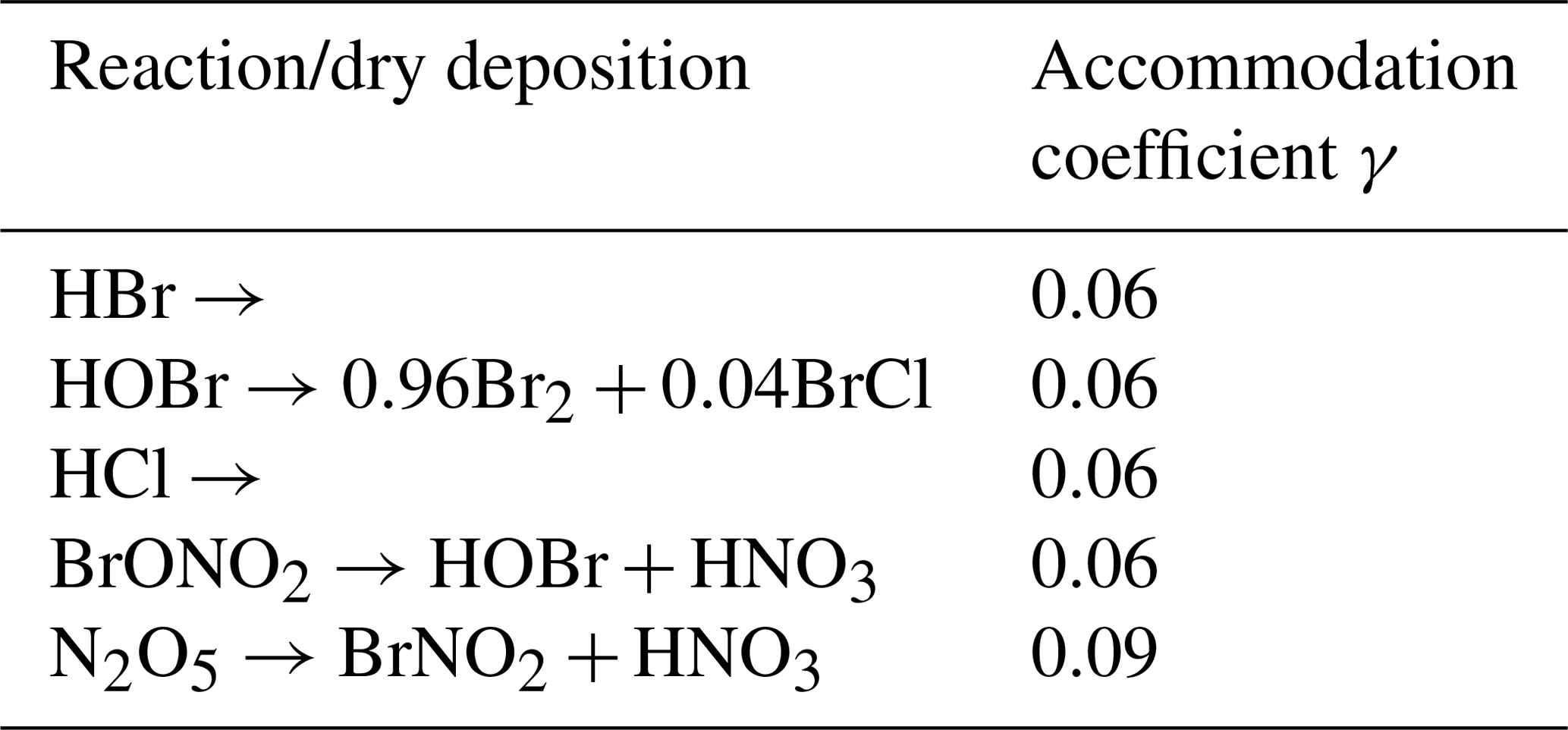
Download Print Version | Download XLSX

Author contributions

MH developed the code that was used to perform the simulations and created all figures presented in the paper. The code is based on previous work of LC, who helped to advance the present more extended code. HS contributed with respect to the model extension and validation of the results. UP and EG devised the methodology and supervised the project. The draft manuscript was edited by MH, and all authors contributed through numerous revisions of the draft paper.

Competing interests

The authors declare that they have no conflict of interest.

Acknowledgements

The authors thank Rolf Sander from the Max Planck Institute for Chemistry, Mainz, Germany, for very fruitful discussions concerning the chemical reaction scheme and the aerosol treatment. The authors gratefully acknowledge funding by the Deutsche Forschungsgemeinschaft (DFG, German Research Foundation) – Projektnummer 85276297 and through HGS MathComp. Le Cao acknowledges funding through the National Natural Science Foundation of China (grant no. 41705103).

Financial support

This research has been funded by the Deutsche Forschungsgemeinschaft (DFG, German Research Foundation) – Projektnummer 85276297 and through HGS MathComp. Le Cao received funding through the National Natural Science Foundation of China (grant no. 41705103).

Review statement

This paper was edited by Laurens Ganzeveld and reviewed by three anonymous referees.

References

Abbatt, J. P. D., Thomas, J. L., Abrahamsson, K., Boxe, C., Granfors, A., Jones, A. E., King, M. D., Saiz-Lopez, A., Shepson, P. B., Sodeau, J., Toohey, D. W., Toubin, C., von Glasow, R., Wren, S. N., and Yang, X.: Halogen activation via interactions with environmental ice and snow in the polar lower troposphere and other regions, Atmos. Chem. Phys., 12, 6237–6271, https://doi.org/10.5194/acp-12-6237-2012, 2012. a

Adams, J. W., Holmes, N. S., and Crowley, J. N.: Uptake and reaction of HOBr on frozen and dry NaCl/NaBr surfaces between 253 and 233 K, Atmos. Chem. Phys., 2, 79–91, https://doi.org/10.5194/acp-2-79-2002, 2002. a

Alfonso, A., Georges, L. B., Gérard, L. V., and Gilles, P.: The BrO+Ch₃O₂ reaction: Kinetics and role in the atmospheric ozone budget, Geophys. Res. Lett., 24, 2745–2748, https://doi.org/10.1029/97GL02686, 1997. a, b

Artiglia, L., Edebeli, J., Orlando, F., Chen, S., Lee, M.-T., Arroyo, P. C., Gilgen, A., Bartels-Rausch, T., Kleibert, A., Vazdar, M., Andres Carignano, M., Francisco, J. S., Shepson, P. B., Gladich, I., and Ammann, M.: A surface-stabilized ozonide triggers bromide oxidation at the aqueous solution-vapour interface, Nat. Commun., 8, 700, https://doi.org/10.1038/s41467-017-00823-x, 2017. a

Atkinson, R., Baulch, D. L., Cox, R. A., Crowley, J. N., Hampson, R. F., Hynes, R. G., Jenkin, M. E., Rossi, M. J., and Troe, J.: Evaluated kinetic and photochemical data for atmospheric chemistry: Volume I – gas phase reactions of O_x, HO_x, NO_x and SO_x species, Atmos. Chem. Phys., 4, 1461–1738, https://doi.org/10.5194/acp-4-1461-2004, 2004. a, b, c, d, e, f, g, h, i, j, k, l, m, n, o, p, q, r, s, t, u, v, w, x, y, z, aa, ab, ac, ad, ae

Atkinson, R., Baulch, D. L., Cox, R. A., Crowley, J. N., Hampson, R. F., Hynes, R. G., Jenkin, M. E., Rossi, M. J., Troe, J., and IUPAC Subcommittee: Evaluated kinetic and photochemical data for atmospheric chemistry: Volume II – gas phase reactions of organic species, Atmos. Chem. Phys., 6, 3625–4055, https://doi.org/10.5194/acp-6-3625-2006, 2006. a, b, c, d, e, f, g, h, i, j, k, l, m, n, o, p, q, r, s, t, u, v, w, x, y, z, aa, ab, ac, ad, ae, af, ag, ah, ai, aj, ak, al, am, an, ao, ap

Atkinson, R., Baulch, D. L., Cox, R. A., Crowley, J. N., Hampson, R. F., Hynes, R. G., Jenkin, M. E., Rossi, M. J., and Troe, J.: Evaluated kinetic and photochemical data for atmospheric chemistry: Volume III – gas phase reactions of inorganic halogens, Atmos. Chem. Phys., 7, 981–1191, https://doi.org/10.5194/acp-7-981-2007, 2007. a, b, c, d, e, f, g, h, i, j, k, l, m, n, o, p, q, r, s, t, u, v, w, x, y, z, aa, ab, ac, ad, ae, af, ag, ah, ai, aj, ak, al, am, an, ao, ap, aq, ar, as, at, au, av, aw, ax, ay, az, ba, bb

Barnes, I., Becker, K. H., and Overath, R. D.: Oxidation of Organic Sulfur Compounds, in: The Tropospheric Chemistry of Ozone in the Polar Regions, edited by: Niki, H. and Becker, K. H., 371–383, Springer Berlin Heidelberg, Berlin, Heidelberg, Germany, 1993. a, b

Barrie, L., Bottenheim, J., Schnell, R., Crutzen, P., and Rasmussen, R.: Ozone destruction and photochemical reactions at polar sunrise in the lower Arctic atmosphere, Nature, 334, 138–141, 1988. a, b

Beine, H. J., Dominè, F., Ianniello, A., Nardino, M., Allegrini, I., Teinilä, K., and Hillamo, R.: Fluxes of nitrates between snow surfaces and the atmosphere in the European high Arctic, Atmos. Chem. Phys., 3, 335–346, https://doi.org/10.5194/acp-3-335-2003, 2003. a

Borken, J.: Ozonabbau durch Halogene in der arktischen Grenzschicht, Master's thesis, Heidelberg University, Heidelberg, Germany, 1996 (in German). a, b, c, d

Bottenheim, J. W. and Chan, E.: A trajectory study into the origin of spring time Arctic boundary layer ozone depletion, J. Geophys. Res.-Atmos., 111, D19301, https://doi.org/10.1029/2006JD007055, 2006. a

Bottenheim, J. W., Gallant, A., and Brice, K.: Measurements of NO_y species and O₃ at 82 N latitude, Geophys. Res. Lett., 13, 113–116, 1986. a, b

Bottenheim, J. W., Netcheva, S., Morin, S., and Nghiem, S. V.: Ozone in the boundary layer air over the Arctic Ocean: measurements during the TARA transpolar drift 2006–2008, Atmos. Chem. Phys., 9, 4545–4557, https://doi.org/10.5194/acp-9-4545-2009, 2009. a

Briggs, T. S. and Rauscher, W. C.: An oscillating iodine clock, J. Chem. Educ., 50, 496–496, https://doi.org/10.1021/ed050p496, 1973. a

Cao, L. and Gutheil, E.: Numerical simulation of tropospheric ozone depletion in the polar spring, Air Qual. Atmos. Hlth., 6, 673–686, 2013. a

Cao, L., Sihler, H., Platt, U., and Gutheil, E.: Numerical analysis of the chemical kinetic mechanisms of ozone depletion and halogen release in the polar troposphere, Atmos. Chem. Phys., 14, 3771–3787, https://doi.org/10.5194/acp-14-3771-2014, 2014. a, b, c

Cao, L., Platt, U., and Gutheil, E.: Role of the boundary layer in the occurrence and termination of the tropospheric ozone depletion events in polar spring, Atmos. Environ., 132, 98–110, 2016. a, b, c, d, e, f, g, h, i, j, k

Chu, L. and Anastasio, C.: Quantum yields of hydroxyl radical and nitrogen dioxide from the photolysis of nitrate on ice, J. Phys. Chem. A, 107, 9594–9602, 2003. a

Cotter, E., Jones, A., Wolff, E., and Bauguitte, S.-B.: What controls photochemical NO and NO₂ production from Antarctic snow? Laboratory investigation assessing the wavelength and temperature dependence, J. Geophys. Res.-Atmos., 108, 4147, https://doi.org/10.1029/2002JD002602, 2003. a

DeMore, W. B., Sander, S. P., Golden, D., Hampson, R., Kurylo, M. J., Howard, C. J., Ravishankara, A., Kolb, C., and Molina, M.: Chemical Kinetics and Photochemical Data for Use in Stratospheric Modeling. Evaluation No. 12, Tech. rep., Jet Propulsion Lab., California Inst. of Tech., Pasadena, CA, USA, 1997. a, b, c

Dubowski, Y., Colussi, A., and Hoffmann, M.: Nitrogen dioxide release in the 302 nm band photolysis of spray-frozen aqueous nitrate solutions. Atmospheric implications, J. Phys. Chem. A, 105, 4928–4932, 2001. a, b

Evans, M. J., Jacob, D. J., Atlas, E., Cantrell, C. A., Eisele, F., Flocke, F., Fried, A., Mauldin, R. L., Ridley, B. A., Wert, B., Talbot, R., Blake, D., Heikes, B., Snow, J., Walega, J., Weinheimer, A. J., and Dibb, J.: Coupled evolution of ${BrO}_{x} - {ClO}_{x} - {HO}_{x} - {NO}_{x}$ chemistry during bromine-catalyzed ozone depletion events in the arctic boundary layer, J. Geophys. Res.-Atmos., 108, 8368, https://doi.org/10.1029/2002JD002732, 2003. a, b, c, d, e, f, g, h, i, j, k, l, m, n, o, p, q, r, s, t, u, v, w, x, y, z, aa, ab, ac, ad, ae, af, ag

Fan, S.-M. and Jacob, D. J.: Surface ozone depletion in Arctic spring sustained by bromine reactions on aerosols, Nature, 359, 522–524, 1992. a

Fox, J. L., Wofsy, S. C., McElroy, M. B., and Prather, M. J.: A stratospheric chemical instability, J. Geophys. Res.-Oceans, 87, 11126–11132, https://doi.org/10.1029/JC087iC13p11126, 1982. a

Frieß, U., Hollwedel, J., König-Langlo, G., Wagner, T., and Platt, U.: Dynamics and chemistry of tropospheric bromine explosion events in the Antarctic coastal region, J. Geophys. Res.-Atmos., 109, D06305, https://doi.org/10.1029/2003JD004133, 2004. a, b

Frieß, U., Sihler, H., Sander, R., Pöhler, D., Yilmaz, S., and Platt, U.: The vertical distribution of BrO and aerosols in the Arctic: Measurements by active and passive differential optical absorption spectroscopy, J. Geophys. Res.-Atmos., 116, D00R04, https://doi.org/10.1029/2011JD015938, 2011. a

Gottwald, B. A. and Wanner, G.: A reliable Rosenbrock integrator for stiff differential equations, Computing, 26, 355–360, https://doi.org/10.1007/BF02237954, 1981. a

Grannas, A. M., Jones, A. E., Dibb, J., Ammann, M., Anastasio, C., Beine, H. J., Bergin, M., Bottenheim, J., Boxe, C. S., Carver, G., Chen, G., Crawford, J. H., Dominé, F., Frey, M. M., Guzmán, M. I., Heard, D. E., Helmig, D., Hoffmann, M. R., Honrath, R. E., Huey, L. G., Hutterli, M., Jacobi, H. W., Klán, P., Lefer, B., McConnell, J., Plane, J., Sander, R., Savarino, J., Shepson, P. B., Simpson, W. R., Sodeau, J. R., von Glasow, R., Weller, R., Wolff, E. W., and Zhu, T.: An overview of snow photochemistry: evidence, mechanisms and impacts, Atmos. Chem. Phys., 7, 4329–4373, https://doi.org/10.5194/acp-7-4329-2007, 2007. a

Grebel, J. E., Pignatello, J. J., and Mitch, W. A.: Effect of halide ions and carbonates on organic contaminant degradation by hydroxyl radical-based advanced oxidation processes in saline waters, Environ. Sci. Technol., 44, 6822–6828, 2010. a

Halfacre, J. W., Knepp, T. N., Shepson, P. B., Thompson, C. R., Pratt, K. A., Li, B., Peterson, P. K., Walsh, S. J., Simpson, W. R., Matrai, P. A., Bottenheim, J. W., Netcheva, S., Perovich, D. K., and Richter, A.: Temporal and spatial characteristics of ozone depletion events from measurements in the Arctic, Atmos. Chem. Phys., 14, 4875–4894, https://doi.org/10.5194/acp-14-4875-2014, 2014. a, b

Hausmann, M. and Platt, U.: Spectroscopic measurement of bromine oxide and ozone in the high Arctic during Polar Sunrise Experiment 1992, J. Geophys. Res.-Atmos., 99, 25399–25413, 1994. a, b, c

Helmig, D., Boylan, P., Johnson, B., Oltmans, S., Fairall, C., Staebler, R., Weinheimer, A., Orlando, J., Knapp, D. J., Montzka, D. D., Flocke, F., Frieß, U., Sihler, H., and Shepson, P. B.: Ozone dynamics and snow-atmosphere exchanges during ozone depletion events at Barrow, Alaska, J. Geophys. Res.-Atmos., 117, D20303, https://doi.org/10.1029/2012JD017531, 2012. a

Hess, P. G. and Madronich, S.: On tropospheric chemical oscillations, J. Geophys. Res.-Atmos., 102, 15949–15965, https://doi.org/10.1029/97JD00526, 1997. a, b

Honrath, R., Guo, S., Peterson, M. C., Dziobak, M., Dibb, J. E., and Arsenault, M.: Photochemical production of gas phase NO_x from ice crystal ${NO}_{3}^{-}$ , J. Geophys. Res.-Atmos., 105, 24183–24190, 2000. a

Hov, Ø., Schmidbauer, N., and Oehme, M.: Light hydrocarbons in the Norwegian Arctic, Atmos. Environ., 23, 2471–2482, 1989. a

Huff, A. K. and Abbatt, J. P.: Gas-Phase Br2 Production in Heterogeneous Reactions of Cl2, HOCl, and BrCl with Halide- Ice Surfaces, J. Phys. Chem. A, 104, 7284–7293, 2000. a, b

Huff, A. K. and Abbatt, J. P.: Kinetics and product yields in the heterogeneous reactions of HOBr with ice surfaces containing NaBr and NaCl, J. Phys. Chem. A, 106, 5279–5287, 2002. a, b, c

Jacobi, H.-W., Morin, S., and Bottenheim, J. W.: Observation of widespread depletion of ozone in the springtime boundary layer of the central Arctic linked to mesoscale synoptic conditions, J. Geophys. Res.-Atmos., 115, D17302, https://doi.org/10.1029/2010JD013940, 2010. a

Jones, A. E., Weller, R., Wolff, E. W., and Jacobi, H. W.: Speciation and rate of photochemical NO and NO₂ production in Antarctic snow, Geophys. Res. Lett., 27, 345–348, https://doi.org/10.1029/1999GL010885, 2000. a

Jones, A. E., Weller, R., Anderson, P. S., Jacobi, H. W., Wolff, E. W., Schrems, O., and Miller, H.: Measurements of NO_x emissions from the Antarctic snowpack, Geophys. Res. Lett., 28, 1499–1502, https://doi.org/10.1029/2000GL011956, 2001. a

Kalachev, L. V. and Field, R. J.: Reduction of a Model Describing Ozone Oscillations in the Troposphere: Example of an Algorithmic Approach to Model Reduction in Atmospheric Chemistry, J. Atmos. Chem., 39, 65–93, https://doi.org/10.1023/A:1010649217616, 2001. a

Keil, A. D. and Shepson, P. B.: Chlorine and bromine atom ratios in the springtime Arctic troposphere as determined from measurements of halogenated volatile organic compounds, J. Geophys. Res.-Atmos., 111, D17303, https://doi.org/10.1029/2006JD007119, 2006. a

Koo, J.-H., Wang, Y., Kurosu, T. P., Chance, K., Rozanov, A., Richter, A., Oltmans, S. J., Thompson, A. M., Hair, J. W., Fenn, M. A., Weinheimer, A. J., Ryerson, T. B., Solberg, S., Huey, L. G., Liao, J., Dibb, J. E., Neuman, J. A., Nowak, J. B., Pierce, R. B., Natarajan, M., and Al-Saadi, J.: Characteristics of tropospheric ozone depletion events in the Arctic spring: analysis of the ARCTAS, ARCPAC, and ARCIONS measurements and satellite BrO observations, Atmos. Chem. Phys., 12, 9909–9922, https://doi.org/10.5194/acp-12-9909-2012, 2012. a

Lehrer, E., Hönninger, G., and Platt, U.: A one dimensional model study of the mechanism of halogen liberation and vertical transport in the polar troposphere, Atmos. Chem. Phys., 4, 2427–2440, https://doi.org/10.5194/acp-4-2427-2004, 2004. a, b, c, d, e, f, g, h, i, j, k, l, m, n, o, p, q, r, s, t

Lotka, A. J.: Contribution to the Theory of Periodic Reactions, J. Phys. Chem., 14, 271–274, https://doi.org/10.1021/j150111a004, 1909. a

Luther, G. W., Swartz, C. B., and Ullman, W. J.: Direct determination of iodide in seawater by cathodic stripping square wave voltammetry, Anal. Chem., 60, 1721–1724, 1988. a

Mallard, W. G., Westley, F., Herron, J., Hampson, R. F., and Frizzell, D.: NIST chemical kinetics database, Version 5.0, National Institute of Standards and Technology, Gaithersburg, MD, USA, 1993. a

McConnell, J., Henderson, G., Barrie, L., Bottenheim, J., Niki, H., Langford, C., and Templeton, E.: Photochemical bromine production implicated in Arctic boundary-layer ozone depletion, Nature, 355, 150–152, 1992. a

Michalowski, B. A., Francisco, J. S., Li, S.-M., Barrie, L. A., Bottenheim, J. W., and Shepson, P. B.: A computer model study of multiphase chemistry in the Arctic boundary layer during polar sunrise, J. Geophys. Res.-Atmos., 105, 15131–15145, 2000. a, b

Millero, F. J., Feistel, R., Wright, D. G., and McDougall, T. J.: The composition of Standard Seawater and the definition of the Reference-Composition Salinity Scale, Deep-Sea Res. Pt. I, 55, 50–72, 2008. a

Moore, C. W., Obrist, D., Steffen, A., Staebler, R. M., Douglas, T. A., Richter, A., and Nghiem, S. V.: Convective forcing of mercury and ozone in the Arctic boundary layer induced by leads in sea ice, Nature, 506, 81–84, 2014. a

Neff, W., Helmig, D., Grachev, A., and Davis, D.: A study of boundary layer behavior associated with high NO concentrations at the South Pole using a minisodar, tethered balloon, and sonic anemometer, Atmos. Environ., 42, 2762–2779, 2008. a, b, c

Nesbitt, F., Monks, P., Payne, W., Stief, L., and Toumi, R.: The reaction O (³P)+ HOBr: Temperature dependence of the rate constant and importance of the reaction as an HOBr stratospheric loss process, Geophys. Res. Lett., 22, 827–830, 1995. a

Oltmans, S.: Surface ozone measurements in clean air, J. Geophys. Res.-Oceans, 86, 1174–1180, https://doi.org/10.1029/JC086iC02p01174, 1981. a

Oltmans, S. J., Johnson, B. J., and Harris, J. M.: Springtime boundary layer ozone depletion at Barrow, Alaska: Meteorological influence, year-to-year variation, and long-term change, J. Geophys. Res.-Atmos., 117, D00R18, https://doi.org/10.1029/2011JD016889, 2012. a

Oum, K., Lakin, M., and Finlayson-Pitts, B.: Bromine activation in the troposphere by the dark reaction of O₃ with seawater ice, Geophys. Res. Lett., 25, 3923–3926, 1998. a

Palo, T., Vihma, T., Jaagus, J., and Jakobson, E.: Observations of temperature inversions over central Arctic sea ice in summer, Q. J. Roy. Meteor. Soc., 143, 2741–2754, 2017. a

Pielke, R. A. and Mahrer, Y.: Representation of the Heated Planetary Boundary Layer in Mesoscale Models with Coarse Vertical Resolution, J. Atmos. Sci., 32, 2288–2308, https://doi.org/10.1175/1520-0469(1975)032<2288:ROTHPB>2.0.CO;2, 1975. a

Platt, U. and Janssen, C.: Observation and role of the free radicals NO₃, ClO, BrO and IO in the troposphere, Faraday Discuss., 100, 175–198, 1995. a, b

Platt, U. and Lehrer, E.: Arctic tropospheric ozone chemistry, ARCTOC, no. 64 in Air pollution research report, European Commission Directorate-General, Science, Research and Development, Luxembourg, 1997. a

Pöhler, D., Vogel, L., Frieß, U., and Platt, U.: Observation of halogen species in the Amundsen Gulf, Arctic, by active long-path differential optical absorption spectroscopy, P. Natl. Acad. Sci. USA, 107, 6582–6587, 2010. a

Poppe, D. and Lustfeld, H.: Nonlinearities in the gas phase chemistry of the troposphere: Oscillating concentrations in a simplified mechanism, J. Geophys. Res.-Atmos., 101, 14373–14380, 1996. a

Pratt, K. A., Custard, K. D., Shepson, P. B., Douglas, T. A., Pöhler, D., General, S., Zielcke, J., Simpson, W. R., Platt, U., Tanner, D. J., Gregory Huey, L., Carlsen, M., and Stirm, B. H.: Photochemical production of molecular bromine in Arctic surface snowpacks, Nat. Geosci., 6, 351–356, https://doi.org/10.1038/ngeo1779, 2013. a, b, c

Pruppacher, H. R., Klett, J. D., and Wang, P. K.: Microphysics of Clouds and Precipitation, Aerosol Sci. Tech., 28, 381–382, https://doi.org/10.1080/02786829808965531, 1998. a

Röth, E.-P.: A fast algorithm to calculate the photonflux in optically dense media for use in photochemical models, Berichte der Bunsengesellschaft für physikalische Chemie, 96, 417–420, 1992. a

Röth, E.-P.: Description of the anisotropic radiation transfer model ART to determine photodissociation coefficients, Inst. für Stratosphärische Chem., Forsch. Julich, Julich, Germany, 2002. a

Saiz-Lopez, A., Mahajan, A. S., Salmon, R. A., Bauguitte, S. J.-B., Jones, A. E., Roscoe, H. K., and Plane, J. M.: Boundary layer halogens in coastal Antarctica, Science, 317, 348–351, 2007. a

Sander, R.: Modeling Atmospheric Chemistry: Interactions between Gas-Phase Species and Liquid Cloud/Aerosol Particles, Surv. Geophys., 20, 1–31, https://doi.org/10.1023/A:1006501706704, 1999. a

Sander, R. and Crutzen, P. J.: Model study indicating halogen activation and ozone destruction in polluted air masses transported to the sea, J. Geophys. Res.-Atmos., 101, 9121–9138, 1996. a

Sander, R., Vogt, R., Harris, G. W., and Crutzen, P. J.: Modelling the chemistry of ozone, halogen compounds, and hydrocarbons in the arctic troposphere during spring, Tellus B, 45, 522–532, https://doi.org/10.3402/tellusb.v45i5.16001, 1997. a, b, c, d, e, f, g, h, i, j

Sander, R., Baumgaertner, A., Gromov, S., Harder, H., Jöckel, P., Kerkweg, A., Kubistin, D., Regelin, E., Riede, H., Sandu, A., Taraborrelli, D., Tost, H., and Xie, Z.-Q.: The atmospheric chemistry box model CAABA/MECCA-3.0, Geosci. Model Dev., 4, 373–380, https://doi.org/10.5194/gmd-4-373-2011, 2011.. a, b, c, d, e, f, g, h, i, j, k

Seinfeld, J. H. and Pandis, S. N.: Atmospheric chemistry and physics: from air pollution to climate change, John Wiley & Sons, New York, USA, 2006. a

Simpson, W. R., Alvarez-Aviles, L., Douglas, T. A., Sturm, M., and Domine, F.: Halogens in the coastal snow pack near Barrow, Alaska: Evidence for active bromine air-snow chemistry during springtime, Geophys. Res. Lett., 32, L04811, https://doi.org/10.1029/2004GL021748, 2005. a

Simpson, W. R., von Glasow, R., Riedel, K., Anderson, P., Ariya, P., Bottenheim, J., Burrows, J., Carpenter, L. J., Frieß, U., Goodsite, M. E., Heard, D., Hutterli, M., Jacobi, H.-W., Kaleschke, L., Neff, B., Plane, J., Platt, U., Richter, A., Roscoe, H., Sander, R., Shepson, P., Sodeau, J., Steffen, A., Wagner, T., and Wolff, E.: Halogens and their role in polar boundary-layer ozone depletion, Atmos. Chem. Phys., 7, 4375–4418, https://doi.org/10.5194/acp-7-4375-2007, 2007. a

Simpson, W. R., Brown, S. S., Saiz-Lopez, A., Thornton, J. A., and von Glasow, R.: Tropospheric halogen chemistry: Sources, cycling, and impacts, Chem. Rev., 115, 4035–4062, 2015. a

Staebler, R. M., den Hartog, G., Georgi, B., and Düsterdiek, T.: Aerosol size distributions in Arctic haze during the Polar Sunrise Experiment 1992, J. Geophys. Res.-Atmos., 99, 25429–25437, https://doi.org/10.1029/94JD00520, 1994. a

Stull, R. B.: An introduction to boundary layer meteorology, vol. 13, Springer Netherlands, https://doi.org/10.1007/978-94-009-3027-8, 1988. a

Tang, J. and McConnell, J.: Surface ozone depletion in Arctic spring sustained by bromine reactions on aerosols, Geophys. Res. Lett., 23, 2633–2636, 1996. a

Tarasick, D. W. and Bottenheim, J. W.: Surface ozone depletion episodes in the Arctic and Antarctic from historical ozonesonde records, Atmos. Chem. Phys., 2, 197–205, https://doi.org/10.5194/acp-2-197-2002, 2002. a

Tinsley, M. R. and Field, R. J.: Steady State Instability and Oscillation in Simplified Models of Tropospheric Chemistry, J. Phys. Chem. A, 105, 11212–11219, https://doi.org/10.1021/jp010571t, 2001. a, b

Toyota, K., Kanaya, Y., Takahashi, M., and Akimoto, H.: A box model study on photochemical interactions between VOCs and reactive halogen species in the marine boundary layer, Atmos. Chem. Phys., 4, 1961–1987, https://doi.org/10.5194/acp-4-1961-2004, 2004. a

Toyota, K., McConnell, J. C., Lupu, A., Neary, L., McLinden, C. A., Richter, A., Kwok, R., Semeniuk, K., Kaminski, J. W., Gong, S.-L., Jarosz, J., Chipperfield, M. P., and Sioris, C. E.: Analysis of reactive bromine production and ozone depletion in the Arctic boundary layer using 3-D simulations with GEM-AQ: inference from synoptic-scale patterns, Atmos. Chem. Phys., 11, 3949–3979, https://doi.org/10.5194/acp-11-3949-2011, 2011. a

Tuckermann, M., Ackermann, R., Gölz, C., Lorenzen-Schmidt, H., Senne, T., Stutz, J., Trost, B., Unold, W., and Platt, U.: DOAS-observation of halogen radical-catalysed arctic boundary layer ozone destruction during the ARCTOC-campaigns 1995 and 1996 in Ny-Ålesund, Spitsbergen, Tellus B, 49, 533–555, https://doi.org/10.3402/tellusb.v49i5.16005, 1997. a

Ueda, H., Fukui, T., Kajino, M., Horiguchi, M., Hashiguchi, H., and Fukao, S.: Eddy diffusivities for momentum and heat in the upper troposphere and lower stratosphere measured by MU radar and RASS, and a comparison of turbulence model predictions, J. Atmos. Sci., 69, 323–337, 2012. a

Wagner, T., Leue, C., Wenig, M., Pfeilsticker, K., and Platt, U.: Spatial and temporal distribution of enhanced boundary layer BrO concentrations measured by the GOME instrument aboard ERS-2, J. Geophys. Res.-Atmos., 106, 24225–24235, 2001. a

Wagner, T., Ibrahim, O., Sinreich, R., Frieß, U., von Glasow, R., and Platt, U.: Enhanced tropospheric BrO over Antarctic sea ice in mid winter observed by MAX-DOAS on board the research vessel Polarstern, Atmos. Chem. Phys., 7, 3129–3142, https://doi.org/10.5194/acp-7-3129-2007, 2007. a

Wennberg, P.: Atmospheric chemistry: Bromine explosion, Nature, 397, 299–301, 1999. a

Wesely, M.: Parameterization of surface resistances to gaseous dry deposition in regional-scale numerical models, Atmos. Environ., 23, 1293–1304, 1989. a

White, W. H. and Dietz, D.: Does the photochemistry of the troposphere admit more than one steady state?, Nature, 309, 242–244, 1984. a

Wilson, R.: Turbulent diffusivity in the free atmosphere inferred from MST radar measurements: a review, Ann. Geophys., 22, 3869–3887, https://doi.org/10.5194/angeo-22-3869-2004, 2004. a

Wren, S. N., Donaldson, D. J., and Abbatt, J. P. D.: Photochemical chlorine and bromine activation from artificial saline snow, Atmos. Chem. Phys., 13, 9789–9800, https://doi.org/10.5194/acp-13-9789-2013, 2013. a, b

Wu, M., Liu, X., Zhang, L., Wu, C., Lu, Z., Ma, P.-L., Wang, H., Tilmes, S., Mahowald, N., Matsui, H., and Easter, R. C.: Impacts of aerosol dry deposition on black carbon spatial distributions and radiative effects in the community atmosphere model CAM5, J. Adv. Model. Earth Sy., 10, 1150–1171, 2018. a

Ye, C., Zhou, X., Pu, D., Stutz, J., Festa, J., Spolaor, M., Tsai, C., Cantrell, C., Mauldin, R. L., Campos, T., Weinheimer, A., Hornbrook, R. S., Apel, E. C., Guenther, A., Kaser, L., Yuan, B., Karl, T., Haggerty, J., Hall, S., Ullmann, K., Smith, J. N., Ortega, J., and Knote, C.: Rapid cycling of reactive nitrogen in the marine boundary layer, Nature, 532, 489–491, 2016. a, b

Zhu, C., Xiang, B., Chu, L. T., and Zhu, L.: 308 nm photolysis of nitric acid in the gas phase, on aluminum surfaces, and on ice films, J. Phys. Chem. A, 114, 2561–2568, 2010. a, b

Articles

Short summary

The oscillations of tropospheric ODEs in the Arctic spring is studied numerically. After the termination of an ODE, the reactive bromine is deposited onto aerosols/the snow surface, and the ozone may regenerate. The replenished ozone is available for the next autocatalytic bromine release, leading to the oscillation of an ODE. Its dependence on the NO_x mixing ratio, the inversion layer strength, the ambient temperature, the aerosol density, and the solar radiation is investigated.

On the contribution of chemical oscillations to ozone depletion events in the polar spring

2.1 The differential equations

2.1.1 Turbulent diffusion coefficient

2.1.2 Chemical reaction mechanism

2.1.3 Treatment of the aerosols

2.2 Numerical aspects of the model

2.2.1 The numerical grid

2.2.2 The numerical solver

2.3 Base parameters

2.4 Initial and boundary conditions

2.4.1 Initial conditions

2.4.2 Boundary conditions and heterogenous reactions at the ice surface

3.1 Oscillation and termination of ODEs

3.1.1 Oscillation of ODEs

3.1.2 Termination of ODE oscillations

3.2 Initialization of an ODE with only aerosols

3.3 Comparison to studies in the literature

3.4 Study of model parameters influencing the oscillation period

3.4.1 Strength of the inversion layer

3.4.2 The role of NOy, T and chlorine

3.4.3 The influence of the aerosol density

3.4.4 Variation of the solar zenith angle

A1 Gas-phase reactions

A2 Photolysis reactions

A3 Gas–aerosol mass transfer constants

A4 Aqueous-phase reactions and equilibria

A5 Heterogenous reactions and dry depositions

3.4.2 The role of NO_y, T and chlorine