the Creative Commons Attribution 4.0 License.
the Creative Commons Attribution 4.0 License.
 | 12 Aug 2019
Transport of Po Valley aerosol pollution to the northwestern Alps – Part 2: Long-term impact on air quality
Gian Paolo Gobbi
Tiziana Magri
Giordano Pession
Sara Pittavino
Ivan K. F. Tombolato
Monica Campanelli
Francesca Barnaba
This work evaluates the impact of trans-regional aerosol transport from the Po basin on particulate matter levels (PM10) and physico-chemical characteristics in the northwestern Alps. To this purpose, we exploited a multi-sensor, multi-platform database over a 3-year period (2015–2017) accompanied by a series of numerical simulations. The experimental setup included operational (24/7) vertically resolved aerosol profiles by an automated lidar ceilometer (ALC), vertically integrated aerosol properties by a Sun/sky photometer, and surface measurements of aerosol mass concentration, size distribution and chemical composition. This experimental set of observations was then complemented by modelling tools, including numerical weather prediction (NWP), trajectory statistical (TSM) and chemical transport (CTM) models, plus positive matrix factorisation (PMF) on both the PM10 chemical speciation analyses and particle size distributions. In a first companion study, we showed and discussed through detailed case studies the 4-D phenomenology of recurrent episodes of aerosol transport from the polluted Po basin to the northwestern Italian Alps. Here we draw more general and statistically significant conclusions on the frequency of occurrence of this phenomenon, and on the quantitative impact of this regular, wind-driven, aerosol-rich “atmospheric tide” on PM10 air-quality levels in this alpine environment. Based on an original ALC-derived classification, we found that an advected aerosol layer is observed at the receptor site (Aosta) in 93 % of days characterized by easterly winds (i.e. from the Po basin) and that the longer the time spent by air masses over the Po plain the higher this probability. Frequency of these advected aerosol layers was found to be rather stable over the seasons with about 50 % of the days affected. Duration of these advection events ranges from few hours up to several days, while aerosol layer thickness ranges from 500 up to 4000 m. Our results confirm this phenomenon to be related to non-local emissions, to act at the regional scale and to largely impact both surface levels and column-integrated aerosol properties. In Aosta, PM10 and aerosol optical depth (AOD) values increase respectively up to factors of 3.5 and 4 in dates under the Po Valley influence. Pollution transport events were also shown to modify the mean chemical composition and typical size of particles in the target region. In fact, increase in secondary species, and mainly nitrate- and sulfate-rich components, were found to be effective proxies of the advections, with the transported aerosol responsible for at least 25 % of the PM10 measured in the urban site of Aosta, and adding up to over 50 µg m−3 during specific episodes, thus exceeding alone the EU established daily limit. From a modelling point of view, our CTM simulations performed over a full year showed that the model is able to reproduce the phenomenon, but markedly underestimates its impact on PM10 levels. As a sensitivity test, we employed the ALC-derived identification of aerosol advections to re-weight the emissions from outside the boundaries of the regional domain in order to match the observed PM10 field. This simplified exercise indicated that an increase in such “external” emissions by a factor of 4 in the model is needed to halve the model PM10 maximum deviations and to significantly reduce the PM10 normalised mean bias forecasts error (from −35 % to 5 %).
- Article
(8142 KB) - Companion paper
-
Supplement
(6564 KB) - BibTeX
- EndNote


Mountain regions are often considered pristine areas, being typically far from large urban settlements and strong anthropogenic emission sources, and thus relatively unaffected by remarkable pollution footprints. However, atmospheric transport of pollutants from the neighbouring foreland is not uncommon, owing to the synoptic and regional circulation patterns. For example, in several regions of the world, thermally driven flows represent a systematic characteristic of mountain weather and climate (Hann, 1879; Thyer, 1966; Kastendeuch and Kaufmann, 1997; Egger et al., 2000; Ying et al., 2009; Serafin and Zardi, 2010; Schmidli, 2013; Zardi and Whiteman, 2013; Wagner et al., 2014a; Giovannini et al., 2017; Schmidli et al., 2018) favouring regular exchange of air masses between the plain and the highland sites (Weissmann et al., 2005; Gohm et al., 2009; Cong et al., 2015; Dhungel et al., 2018), with likely consequences on human health (Loomis et al., 2013; EEA, 2015; WHO, 2016), ecosystems (e.g. Carslaw et al., 2010; EMEP, 2016; Bourgeois et al., 2018; Burkhardt et al., 2018; Allen et al., 2019; Ambrosini et al., 2019; Rizzi et al., 2019), climate (Ramanathan et al., 2001; Clerici and Mélin, 2008; Philipona, 2013; Pepin et al., 2015; Zeng et al., 2015; Tudoroiu et al., 2016; Samset, 2018) and, not least, local economy, through loss of tourism revenues (de Freitas, 2003; Keiser et al., 2018). These phenomena have worldwide relevance, since nearly one-quarter of the Earth's land mass can be classified as mountainous areas (Blyth, 2002).
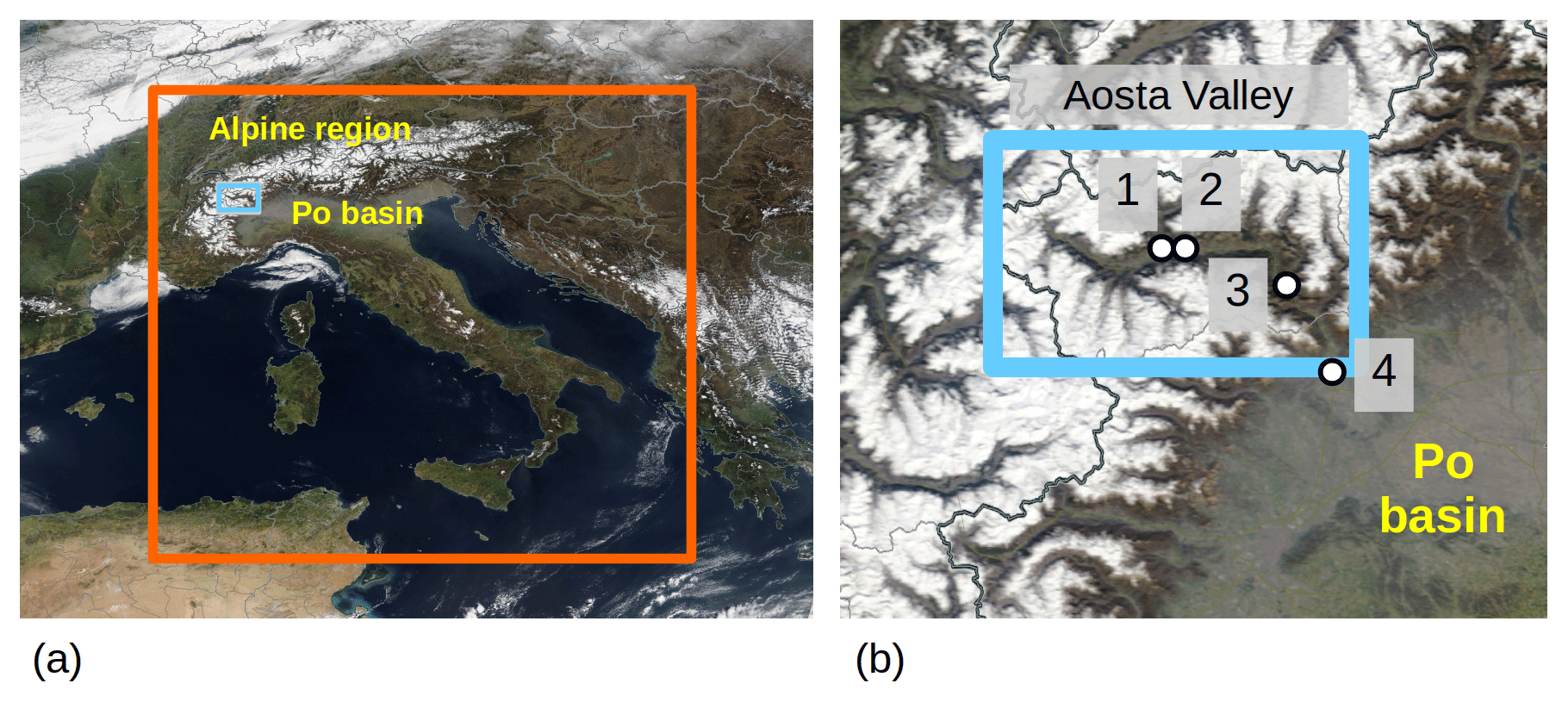
Figure 1True colour corrected reflectance from the MODIS Terra satellite (http://worldview.earthdata.nasa.gov, last access: 2 August 2019) on 17 March 2017. (a) Italy, with indication of the Alpine and Po Valley regions, of the Aosta Valley FARM regional domain (light blue rectangle), and the COSMO-I2 domain (orange rectangle, approximately corresponding to the boundaries of the national inventory). (b) Zoom over the Aosta Valley. The circle markers represent the sites of (1) Aosta–Downtown; (2) Aosta–Saint-Christophe; (3) Donnas; (4) Ivrea. A thin aerosol layer over the Po basin starting to spread out into the Alpine valleys is visible in both figures.
Among them, the Alpine region (Fig. 1a) is of particular interest, due to both its sensitive environment and its proximity to the Po Valley (Tampieri et al., 1981; Seibert et al., 1998; Wotawa et al., 2000; Dosio et al., 2002; Campana et al., 2005; Kaiser, 2009; Finardi et al., 2014). In fact, the Po basin represents a major pollution hotspot in Europe, with large emissions from highly populated urban areas (about 40 % of the Italian population lives in this region, WMO, 2012), intense anthropogenic activities, such as industry and agriculture, combined with a local topography promoting atmospheric stability (Chu et al., 2003; Barnaba and Gobbi, 2004; Schaap et al., 2004; Van Donkelaar et al., 2010; Bigi and Ghermandi, 2014; Fuzzi et al., 2015; EMEP, 2016; Belis et al., 2017; EEA, 2017). Despite the efforts to decrease the number of particulate matter (PM) exceedances, Italy is still failing to comply with the European air-quality standards (EU Commission, 2008, 2018), the Po Valley being the major area responsible for this situation.
In a first companion paper (Diémoz et al., 2019), we investigated the phenomenology of the aerosol-rich air mass advections from the Po basin to the northwestern Alps, and specifically to the Aosta Valley (Fig. 1b). This was introduced and thoroughly described by means of three specifically selected case studies, each of them lasting several days and monitored by a large set of instruments. That investigation evidenced clear features of this phenomenology, and notably,
-
the aerosol transported to the northwestern Alps is clearly detectable and discernible from the locally produced aerosol. Detection of such polluted aerosol layers over Aosta was primarily driven by remote-sensing profiling measurements (automated lidar ceilometers, ALCs), these showing recurrent arrival of thick and elevated aerosol-rich layers. Good correspondence was found between the presence of these layers aloft, changes in column-averaged aerosol properties, and variations of PM surface concentrations and chemical composition;
-
the advected particles are small (accumulation mode), mainly of secondary origin, weakly light-absorbing, and highly hygroscopic compared to the locally produced aerosol. Clouds are frequently observed to form within these layers during the night;
-
the air masses associated with the observed elevated layers are found to originate from the Po basin and to be transported to the northwestern Alps by up-valley diurnal wind systems and synoptic winds;
-
the chemical transport model (FARM, Flexible Air quality Regional Model) currently used by the local Environment Protection Agency (ARPA Valle d'Aosta) is able to reproduce this transport from a qualitative point of view and was usefully employed to interpret the observations. However, it fails at quantitatively estimating the PM mass contribution coming from outside the boundaries of the regional domain (approximately corresponding to the Valle d'Aosta region), likely due to deficiencies in the emission inventories therein and to unaccounted aerosol processes in the model (e.g. those related to hygroscopicity/aqueous-phase chemistry triggered by high relative humidities).
The present work analyses the same phenomenon, but with a long-term perspective. The main aim of this study is to establish the frequency of occurrence of aerosol transport from the Po Valley to the northwestern Alps and its impact on local air quality, depending on the interplay between frequency and severity of the episodes. In particular, this paper addresses the following questions.
-
How frequently does advection from the Po plain to the northwestern Alps occur? What are the most common meteorological conditions favouring it?
-
What are the average properties of the advected aerosol, both at the surface and in the layers aloft?
-
How much does transport from the Po basin impact the air-quality EU-regulated metrics in the northwestern Alps?
-
Can we effectively predict the arrival of aerosol-polluted air masses in the northwestern Alps? How can we improve our air-quality forecasts?
To answer these questions, we took advantage of long-term (2015–2017) and almost uninterrupted series of measurements carried out in the Aosta region. The experimental dataset, thoroughly described by Diémoz et al. (2019), included measurements of vertically resolved aerosol profiles by an ALC, vertically integrated aerosol properties by a Sun/sky photometer, and surface measurements of the aerosol mass concentration, size distribution, and chemical composition, most of these series encompassing a time period of several years. Indeed, a great number of intensive, short-term campaigns employing cutting-edge research instruments and techniques were already performed in the Po basin, mainly focussing on its central, eastern, and southern parts (Nyeki et al., 2002; Barnaba et al., 2007; Ferrero et al., 2010, 2014; Saarikoski et al., 2012; Landi et al., 2013; Decesari et al., 2014; Costabile et al., 2017; Bucci et al., 2018; Cugerone et al., 2018). However, continuous and multi-year datasets, especially from ground-based stations, are necessary to assess the influence of pollution transport on a longer term (e.g. Mélin and Zibordi, 2005; Clerici and Mélin, 2008; Kambezidis and Kaskaoutis, 2008; Mazzola et al., 2010; Bigi and Ghermandi, 2014, 2016; Putaud et al., 2014; Arvani et al., 2016). In this context, local environmental agencies operate stable networks for continuous monitoring of air-quality and meteorological parameters, and use standardised methodologies and universally recognised quality control procedures.
The study is organised as follows: the investigated area is presented in Sect. 2, together with the experimental setup and the modelling tools (Sect. 3). Results are presented in Sect. 4 and include (a) a first, original classification framework based on ALC data and meteorological variables; (b) a long-term, statistical analysis of the phenomenon and its impacts on surface/column aerosol properties; and (c) comparison between observations and CTM simulations. Conclusions are drawn in Sect. 5.
We provide here a brief overview of the region of interest and of the experimental setup, the latter being described with full details in the companion paper (Diémoz et al., 2019).
The Aosta Valley, located at the northwestern Italian border (Fig. 1a), is the smallest administrative region of the country, being only 80 km by 40 km wide and hosting 130 000 inhabitants. The most remarkable geographical feature of the region, whose mean altitude exceeds 2000 m a.s.l., is the main valley, approximately oriented in a SE-to-NW direction and connecting the Po basin (about 300 m a.s.l. at the southeastern side of the Aosta Valley region) to the Mont Blanc chain (4810 m a.s.l., separating Italy and France). Several tributary valleys depart from the main valley. The topography of the area triggers some of the most common weather regimes in the mountains, such as thermally driven, up-valley (daytime), and down-valley (nighttime) winds, up-slope (daytime) and down-slope (nighttime) winds, “Foehn” winds (Seibert, 2012) from the west, and frequent temperature inversions during wintertime anticyclonic days. Quite obviously, those meteorological phenomena are responsible for most of the variability of the tropospheric constituents (e.g. pollutant concentrations, Agnesod et al., 2003, and water vapour, Campanelli et al., 2018).
The air-quality network of the regional Environmental Protection Agency is designed trying to capture the topographical and meteorological heterogeneity of the investigated area. In this study, we mainly used data from four sites belonging to this network (Fig. 1b): Aosta–Downtown (580 m a.s.l., urban background), Aosta–Saint-Christophe (560 m a.s.l., semi-rural), Donnas (316 m a.s.l., rural) and Ivrea (243 m a.s.l., urban background). The first two measuring stations, located 2.5 km apart, are situated respectively in the centre and in the suburbs of Aosta (45.7∘ N, 7.4∘ E), the main urban settlement of the region (36 000 inhabitants). Car traffic, domestic heating and a steel mill are the main anthropogenic emission sources within the city, whose pollution levels are generally moderate (e.g. yearly average PM10 concentration of about 20 µg m−3, with summertime and wintertime averages of 13 and 31 µg m−3 respectively). Donnas is closer to the border with the Po basin (Fig. 1b) and is expected to be strongly impacted by pollution from outside the region. In fact, the PM10 concentration in this rural site is about 18 µg m−3 on a yearly average, i.e. only slightly lower than the concentration in Aosta. We also consider in our analysis the PM10 records collected in the city of Ivrea, a site in the Po Plain (31 µg m−3 average PM10 in 2017) located just outside the Aosta Valley, in the Italian Piedmont region (Fig. 1b). This was done to check whether and how much inaccuracies of the model in reproducing the aerosol loads over the Aosta Valley are due to difficulties in simulating the wind field in such a complex terrain. In fact, the city centre of Ivrea (24 000 inhabitants) is approximately in the middle between the measurement site (south of the city) and the nearest cell of our model domain (north of the city), the distance between these two points being only 2 km. The altitude of the cell (from the digital elevation model used in our simulations) is 241 m a.s.l., i.e. approximately the real one.
Aosta–Downtown hosts a monitoring station for continuous measurements of the aerosol concentration and composition. PM10 and PM2.5 daily concentrations are available from two Opsis SM200 Particulate Monitor instruments. An estimate of the PM10 hourly variability is furthermore provided by a Tapered Element Oscillating Microbalance (TEOM) 1400a monitor (Patashnick and Rupprecht, 1991), but is not compensated for mass loss of semi-volatile compounds (Green et al., 2009) such as ammonium nitrate (e.g. Charron et al., 2004; Rosati et al., 2016). Moreover, the collected PM10 samples are chemically analysed on a daily basis. Ion chromatography (AQUION/ICS-1000 modules) is employed for determining the concentration of water-soluble anions and cations (Cl−, , , Na+, , K+, Mg2+, Ca2+), based on the CEN/TR 16269:2011 guideline. Elemental/organic carbon (EC/OC), using the thermal–optical transmission (TOT) method (Birch and Cary, 1996) and following the EUSAAR-2 protocol (Cavalli et al., 2010) according to the EN 16909:2017, are analysed alternatively to metal concentrations (Cr, Cu, Fe, Mn, Ni, Pb, Zn, As, Cd, Mo, and Co) by means of inductively coupled plasma mass spectrometry (ICP-MS) after acid mineralisation of the filter in aqueous solution (EN 14902:2005). In accordance with this laboratory schedule (i.e. metal analyses on 2 consecutive days, EC/OC on the following 2 days, followed by two sequences metal–metal–EC/OC), over a 10 d period EC/OC concentrations are routinely provided on 4 d on average and metal concentrations on 6 d. Particle-bound polycyclic aromatic hydrocarbons (PAHs) are detected continuously in real time by a photoelectric aerosol sensor (EcoChem PAS-2000). Gas-phase pollutants, such as NO and NO2, are also continuously monitored and were used in the present work to help identification of urban combustion sources (mainly traffic and residential heating).
The atmospheric observatory in Aosta–Saint-Christophe (WIGOS ID 0-380-5-1, Diémoz et al., 2011, 2014a) is located on the terrace of the ARPA building. At this site, advanced instrumentation is continuously operated, checked daily, and maintained. Vertically resolved measurements of aerosols and clouds are performed by a commercially available automated lidar ceilometer (ALC, Lufft CHM15k-Nimbus) running since 2015 in the framework of the Italian Alice-net (http://www.alice-net.eu/, last access: 2 August 2019) and European E-PROFILE (https://e-profile.eu, last access: 2 August 2019) networks. The ALC emits into the atmosphere 8 µJ laser impulses at a single wavelength of 1064 nm with a frequency of 7 kHz and collects their backscatter by aerosol and molecules from the ground up to an altitude of 15 km, with a vertical resolution of 15 m. This return signal is averaged over 15 s and saved by the firmware as range-, overlap-, and baseline-corrected raw counts (βraw). To convert the backscatter signal into SI units, a Rayleigh calibration (Fernald, 1984; Klett, 1985; Wiegner and Geiß, 2012) is necessary. This is accomplished based on data sampled during clear-sky nights. This allows us to derive the particle backscatter coefficient (βp) and the scattering ratio (SR, e.g. Zuev et al., 2017), which is the primary, ALC-derived parameter used in this work to quantify the aerosol load. It is defined as
βm being the molecular backscattering coefficient (thus SR =1 indicates a purely molecular atmosphere while SR increases with aerosol content).
At the same station, a POM-02 Sun/sky photometer has operated since 2012 as part of the European ESR-SKYNET network (http://www.euroskyrad.net/, last access: 2 August 2019). The instrument collects the direct light coming from the Sun (every 1 min) to retrieve the aerosol optical depth (AOD, τ(λ)) and its spectral dependence, calculated by fitting the Ångström (1929) law to the measurements in the 400–870 nm range:
a being the Ångström exponent. Other aerosol optical and microphysical properties are retrieved from the light scattered from the sky in the almucantar plane (every 10 min) at 11 wavelengths (315–2200 nm) using the SKYRAD.pack version 4 code. The Sun photometer is calibrated in situ with the improved Langley technique (Campanelli et al., 2007) and was recently successfully compared to other reference instruments (Kazadzis et al., 2018). Accurate cloud screening is achieved using the Cloud Screening of Sky Radiometer data (CSSR) algorithm by Khatri and Takamura (2009). Special care is needed to retrieve, among the other parameters, the aerosol single scattering albedo (SSA). In fact, it is known that the SSA retrieval by the SKYRAD.pack version 4 is problematic and sometimes unnaturally close to unity (Hashimoto et al., 2012), independently of the AOD. Although improvements are expected in the next versions of SKYRAD.pack, data collected within the European ESR-SKYNET network are still processed with version 4. Therefore, only SSAs lower than 0.99 at all wavelengths were retained in our analysis.
Finally, a Fidas 200s Optical Particle Counter (OPC) is used in Aosta–Saint-Christophe to yield an accurate estimation of the aerosol size distribution (0.18–18 µm) in the proximity of the surface (Pletscher et al., 2016). This instrument, although not directly measuring the aerosol mass, obtained the certificate of equivalence to the gravimetric method by TÜV Rheinland Energy GmbH on the basis of a laboratory test and a field test. A PM10 comparison with the gravimetric technique was additionally performed in Aosta–Saint-Christophe and provided satisfactory results (29 d; slope 1.08±0.04; intercept µg m−3; R2=0.96). Further instruments to monitor trace gases (Diémoz et al., 2014b) are employed at the station and the corresponding datasets will be investigated in future studies.
Some of the air-quality parameters monitored in Aosta–Downtown are also measured at the Donnas station, i.e. PM10 daily concentrations (Opsis SM200) and nitrogen oxides (Horiba APNA-370 chemiluminescence monitor). Finally, the three stations are equipped with instruments for tracking the standard meteorological parameters, such as temperature, pressure, relative humidity (RH), and surface wind velocity.
The station of Ivrea features, among other instruments, a TCR Tecora Charlie/Sentinel PM10 sampler. PM10 concentrations are then determined by a gravimetric technique.
A list of all measurements with relevant operating period and subset considered in this study is presented in Table 1.
Table 1Observation sites, measurements, and instruments employed in this study.
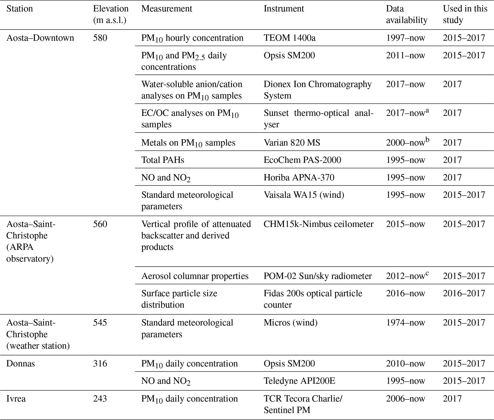
a The analysis is performed on 4 out of 10 d according to the laboratory schedule. b The analysis is performed on 6 out of 10 d according to the laboratory schedule. c Underwent major maintenance in the second half of 2016 and January 2017.
Numerical models and statistical techniques were used to interpret and complement the observations described above. A numerical weather prediction model (COSMO, Consortium for Small-scale Modeling, http://www.cosmo-model.org, last access: 2 August 2019) was employed to drive a chemical transport model (FARM, Flexible Air quality Regional Model) and a Lagrangian model (LAGRANTO). These tools were thoroughly described by Diémoz et al. (2019) and are only briefly recalled here (Sect. 3.1). Trajectory statistical models (TSMs) and positive matrix factorisation (PMF), adopted to interpret the long-term series of measurements used in this work, are fully described in Sects. 3.2 and 3.3 respectively.
3.1 Numerical atmospheric models
COSMO is a non-hydrostatic, fully compressible atmospheric prediction model working on the meso-β and meso-γ scales (Baldauf et al., 2011). The forecasts, inclusive of the complete set of parameters (such as the 3-D wind velocity used here) for eight time steps (from 00:00 to 21:00 UTC), are disseminated daily in two different configurations by the meteorological operative centre–air force meteorological service (COMET): a lower-resolution version (COSMO-ME, 7 km horizontal grid and 45 levels vertical grid, 72 h integration), covering central and southern Europe, and a nudged, higher-resolution version (COSMO-I2 or COSMO-IT, 2.8 km, 65 vertical levels, 2 runs d−1), covering Italy (orange rectangle in Fig. 1a). Owing to the complex topography of the Aosta Valley, and the consequent need to resolve as much as possible the atmospheric circulation at small spatial scales, we used the latter version in the present work (cf. Sect. 4.5 for a discussion of possible effects of the finite model resolution in complex terrain).
FARM version 4.7 (Gariazzo et al., 2007; Silibello et al., 2008; Cesaroni et al., 2013; Calori et al., 2014) is a four-dimensional Eulerian model for simulating the transport, chemical conversion, and deposition of atmospheric pollutants with a 1 km spatial grid, 1 h temporal resolution, and 16 different vertical levels (from the surface to 9290 m). FARM can be easily interfaced to most available diagnostic or prognostic numerical weather prediction (NWP) models, as done with COSMO in the present work. Pollutant emissions from both area and point sources can be simulated by FARM, taking into account transformation of chemical species by gas-phase chemistry and dry and wet removal. Particularly interesting for our study is the aerosol module (AERO3_NEW), coupled with the gas-phase chemical model and treating primary and secondary particle dynamics and their interactions with gas-phase species, thus accounting for nucleation, condensational growth, and coagulation (Binkowski, 1999). Three particle size modes are simulated independently: the Aitken mode (diameter, D<0.1 µm), the accumulation mode (0.1 µm µm), and the coarse mode (D>2.5 µm). FARM is only run over a small domain (light-blue rectangle in Fig. 1a, b) roughly corresponding to the Aosta Valley. A regional emission inventory (“local sources”, updated to 2015) is supplied to the CTM over the same area to accurately assess the magnitude of the pollution load and its variability in time and space. Data from a national inventory and CTM (QualeAria, here referred to as “boundary conditions”, outer rectangle in Fig. 1a), taken along the border of the inner (light blue) rectangle, are also used to estimate the mass exchange from outside the borders of the FARM domain.
3.2 Trajectory statistical models
The forecasted wind velocity profile from COSMO was here used as an input parameter into the publicly available LAGRANTO Lagrangian analysis tool, version 2.0 (Sprenger and Wernli, 2015), to numerically integrate the 3-D wind fields and to determine the origin of the air masses sampled by the ALC over Aosta–Saint-Christophe. We set up the program to start an ensemble of 8 trajectories in a circle of 1 km around the observing site and at seven different altitudes from the ground to 4000 m a.s.l., for a total of 56 trajectories per run. A backward run time of 48 h was considered sufficient, on average, to cover most of the domain of the meteorological model while minimising the numerical errors.
Back-trajectories calculated with LAGRANTO were then employed in TSMs to provide a general picture of the geographical distribution of the probable aerosol sources. In this broadly used technique, the NWP domain is divided into grid cells (i and j indices), and air parcels arriving at a specific receptor site are analysed. When a cell ij is crossed by a back-trajectory l, the tracer concentration cl measured at the arrival point of that trajectory (receptor) is considered. Finally, for each cell, a weighted average Pij is calculated as follows to yield a map of the possible source areas (e.g. Kabashnikov et al., 2011):
where L is the total number of trajectories and τij is the time spent by the trajectory l in the grid cell ij. F(cl) is a function of the concentration at the receptor, and, depending on the chosen technique, can be the concentration itself (concentration-weighted trajectory (CWT) method, e.g. Hsu et al., 2003), the logarithm of the concentration (concentration field (CF) method, Seibert et al., 1994), or the Heaviside step function H(cl−cT), where cT is a concentration threshold (potential source contribution function (PSCF) method, e.g. Ashbaugh et al., 1985), generally the 75th percentile of the concentration series. In this last case, Pij can be statistically interpreted as the conditional probability that concentrations above the threshold cT at the receptor site are related to the passage of the relative back-trajectory through the location ij (e.g. Squizzato and Masiol, 2015). Additional iterative methods exist to reduce trailing effects and to better identify pollution hotspots (e.g. Stohl, 1996). Moreover, the obtained field Pij can be further weighted as a function of the number of trajectories passing through each cell, thus reducing the impact of cells with limited statistics (Zeng and Hopke, 1989).
Any series of atmospheric measurements can be used as the concentration variable cl in Eq. (3). In this work, we achieved especially meaningful results employing the scores from the PMF decomposition (Sect. 3.3), i.e. the contributions of the identified sources to the PM10 daily concentration measured at Aosta–Downtown. The same approach, coupling PMF and TSMs, was employed in other recent studies (e.g. Bressi et al., 2014; Waked et al., 2014; Zong et al., 2018). However, since only daily average information is available from the chemical speciation, the PMF output was repeated eight times per day in order to allow correspondence to the eight back-trajectories per day issued by COSMO and LAGRANTO. We present here results obtained with CF, having checked that application of CWT and PSCF methods provides similar outcomes. The COSMO-I2 domain was thus divided into 130×90 grid cells and 48 h back-trajectories were considered. Only points of the back-trajectories at altitudes lower than 2000 m a.s.l. were taken into account, this being the approximate average height of the mixing layer in the Po basin (Diémoz et al., 2019). Similarly, since the arriving air parcels should be able to impact surface PM levels, only trajectories ending close to the surface over Aosta were examined (i.e. altitudes <1500 m a.s.l., the model surface altitude in the Aosta area being about 900 m a.s.l.). To reduce statistical noise, every value Pij of the resulting map was then multiplied by a weighting factor, wij, linearly varying from 0 (for Nij≤20 end points in a cell) to 1 (for Nij≥200), i.e. . To provide an idea of the effect of this weighting procedure, TSM maps without any weighting (i.e. wij=1) have been included in the Supplement (Fig. S7).
3.3 Positive matrix factorisation
The positive matrix factorisation (PMF, Paatero and Tapper, 1994; Paatero, 1997) technique, as implemented in the US EPA PMF5.0 software (Norris and Duvall, 2014), was employed to study the 2017 series of aerosol chemical analyses and air-quality measurements in Aosta–Downtown. The method allowed us to identify the possible emission sources of the observed aerosol and notably to discriminate its local and non-local origin. PMF requires a long multivariate series of chemical analyses, matrix X (n×m the n rows being the samples and m columns representing the chemical species), and decomposes it into the product of two positive-definite matrices, i.e. G (n×p, matrix of factor contributions, p being the number of factors chosen for the decomposition) and F (p×m, matrix of factor profiles) plus residuals (matrix E):
A solution is found by minimizing the so-called objective function Q, i.e. the squared sum of E, weighted by the measurement uncertainties. A total of 100 runs were performed in this work for each dataset to find an optimal solution. Here we considered three different datasets X: (a) the overall dataset of anion/cation analyses (data available almost every day in 2017, n=360, “PMF dataset a”), (b) a subset of dataset (a), selecting those measurements also having coincident EC/OC analyses (n=132, “PMF dataset b”), and (c) a subset of (a), selecting those measurements also having coincident metal speciation (n=209, “PMF dataset c”). To make the decomposition of the three series comparable, an “unidentified” contribution, corresponding to the carbonaceous species only included in PMF dataset b, was added to PMF datasets a and c. This was done in the following way: we first estimated the total mass of crustal elements using the measured water-soluble calcium concentration as a proxy, with an empirical conversion factor of 10 (e.g. Waked et al., 2014, note that a more rigorous estimate for the soil component was obtained from the PMF analysis itself and confirmed this factor); we then subtracted the sum of the available chemical components (including the estimated mass from soil components) from the total measured PM10 concentration, thus closing the mass balance. This difference was then added in PMF datasets a and c as the “unidentified” source.
Finally, NO, NO2, and total PAHs measured at the same site (Aosta–Downtown) were included in the PMF to help identification of local pollution sources. The number of factors for each dataset was chosen based on physical interpretability of the resulting factors (Sect. S4) and on the Q∕Qexp ratio. The latter is the ratio between the objective function obtained with the selected number of factors (Q, introduced before) and its expected value (Qexp). Elevated (i.e. >2) Q∕Qexp ratios could indicate that some samples and/or species are not well modelled and could be better explained by adding another source (Norris and Duvall, 2014). The measured PM10 concentration was selected as the total variable to determine the contribution of each mode to the PM10 concentration.
PMF was additionally performed on volume size distributions measured by the Fidas OPC in Aosta–Saint-Christophe (Sect. 4.3.3), the m columns representing particle sizes instead of chemical species.
4.1 Daily classification schemes based on ALC measurements or meteorology
Information on the vertical dimension obtained by the ALC was a key factor in identifying the events of aerosol pollution transport over the northwestern Alps (e.g. Diémoz et al., 2019). Therefore, a first step of our analysis was to set up a classification scheme of those advection dates based on ALC measurements. To this purpose, we used the longest ALC record available (2015–2017) and coupled it to meteorological measurements/forecasts. Since, to our knowledge, no previous ALC-based classification method is available in the scientific literature, we defined an original, daily resolved classification scheme based on ceilometer measurements to group dates according to specific ALC-observed conditions. A graphical overview with examples for each class identified is given in Fig. 2. Overall, we identified six classes (A–F) of days:
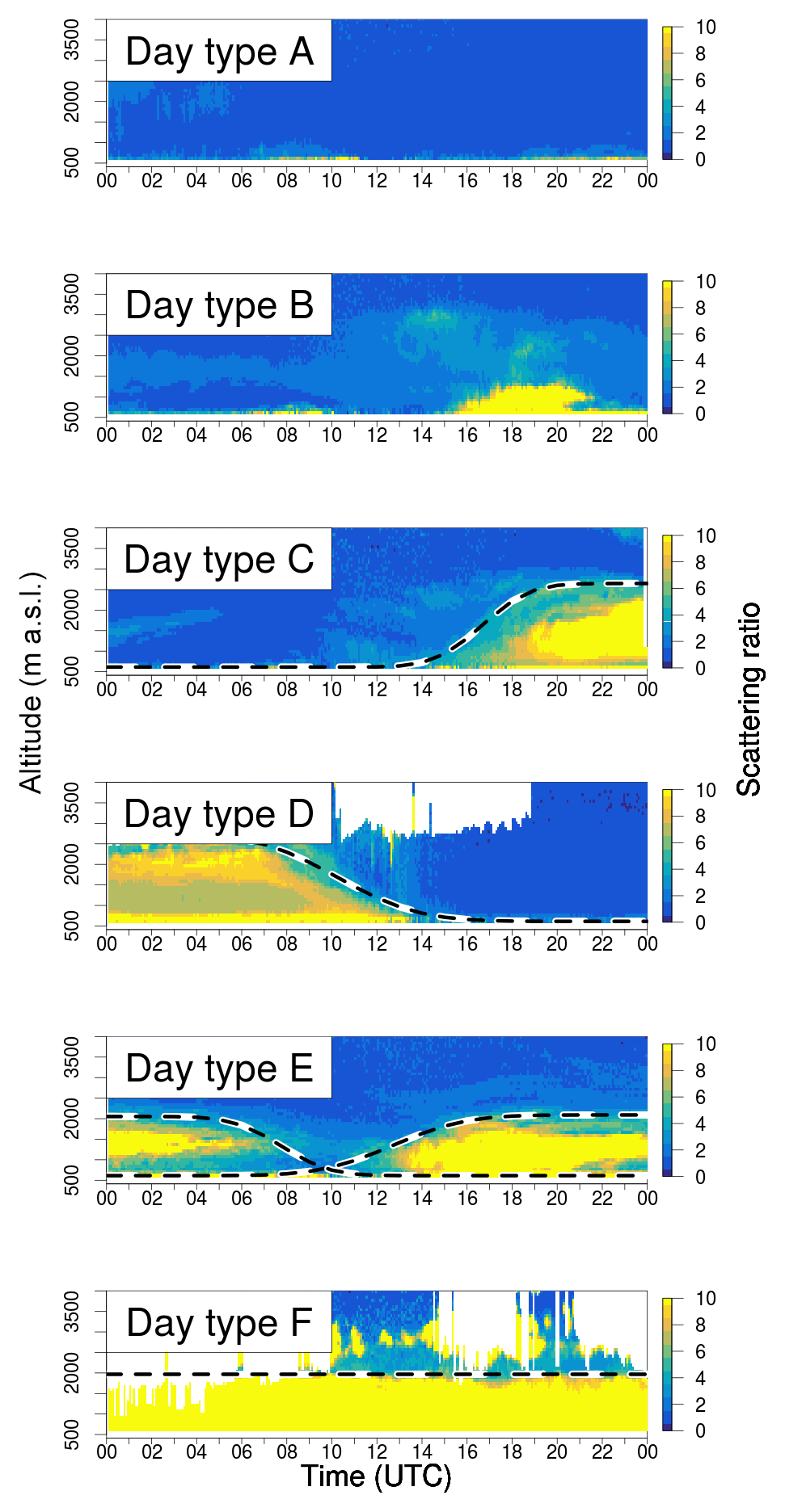
Figure 2Example of ALC images representative of each category (A–F) described in Sect. 4.1. The corresponding dates are 1 December 2015, 19 October 2016, 20 April 2016, 11 April 2015, 1 November 2017, and 27 January 2017. The dashed lines for categories C–F identify the sigmoid interpolation to the SR =3 envelope using the automated algorithm as explained in Sect. 4.2.
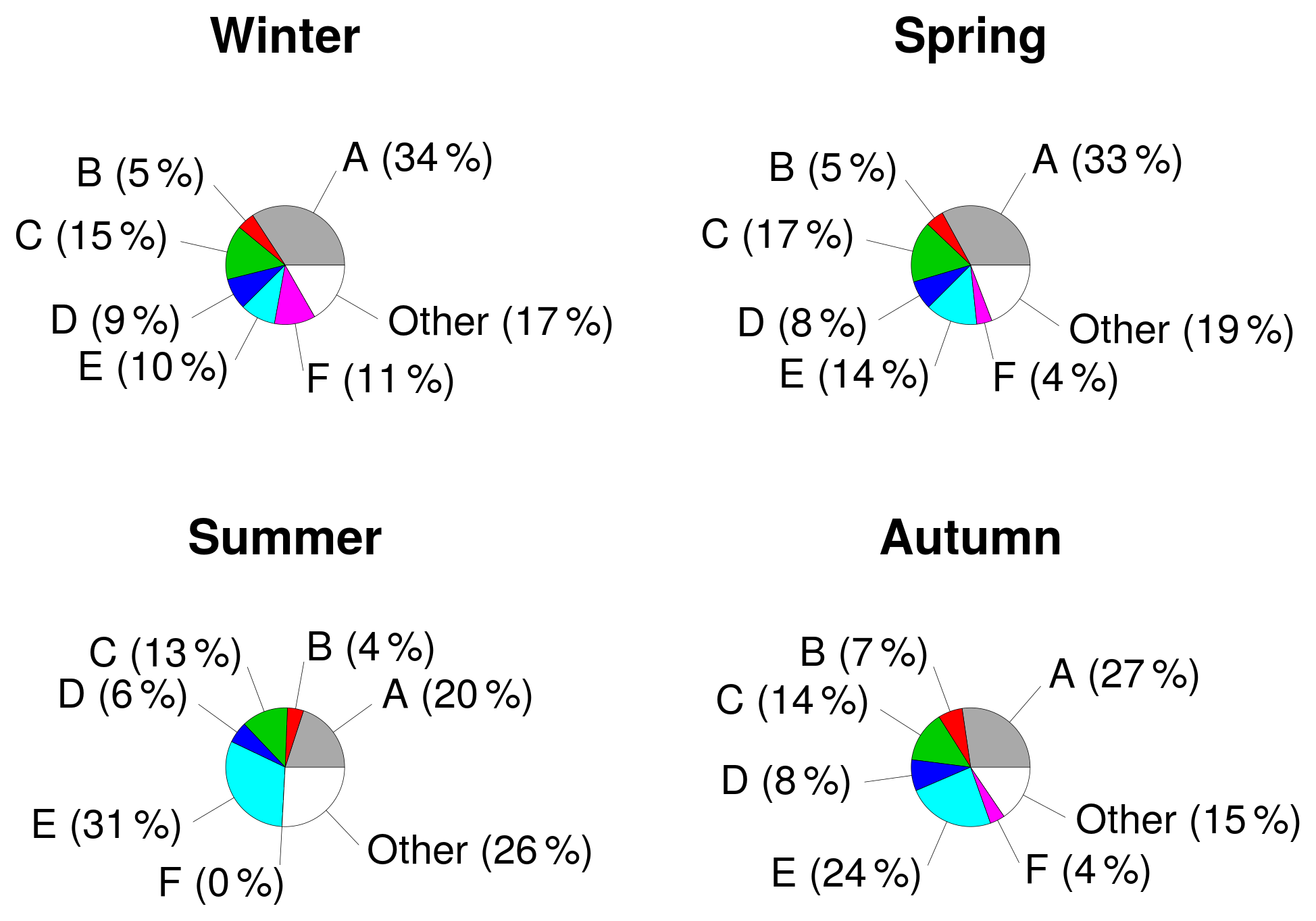
Figure 3Frequency distribution of the aerosol layers observed in Aosta–Saint-Christophe based on the ALC classification described in Sect. 4.1. A: no layer, B: short episodes, C: layer detected in the afternoon, D: leaving layer, E: layer dissolving in the morning and a separated structure in the afternoon, and F: persistent layer.
-
days “A”: no aerosol layer or only low (i.e. <500 m from the ground) aerosol layers visible for the whole day. These days are intended to represent unpolluted conditions or cases only affected by local sources, since aerosol transport from remote regions generally manifests as more elevated layers, as found by Diémoz et al. (2019);
-
days “B”: only brief episodes of layers developing from the surface to altitudes >500 m a.g.l. observed during the 24 h. The origin of the aerosol layers of this intermediate class is uncertain, since they could either result from weak (not completely developed) advections from outside the investigated region or from puffs of locally produced aerosol. For this reason, data in class “B” were used only as a transitional level, but not to draw definitive conclusions;
-
days “C”: detection of an elevated, well-developed aerosol layer (usually in the afternoon) and persistent during the night;
-
days “D”: detection of the aerosol layer from the previous day dissolving during the morning hours. No layers in the afternoon;
-
days “E”: detection of a first aerosol layer from the previous day dissolving (or strongly reducing) in the morning and appearance of a separated structure in the afternoon;
-
days “F”: thick aerosol layer persisting all day long.
Note that, although we also developed automatic recognition algorithms for classification purposes, we finally chose a classification based on visual inspection (for a total of 928 daily images over the 3-year period) to ensure the maximum quality of the flagging and avoid further sources of error.
Table 2Classification of weather regimes used in the study, based on wind speed (), wind direction, daily duration of the condition (Δt), and other measured meteorological variables.
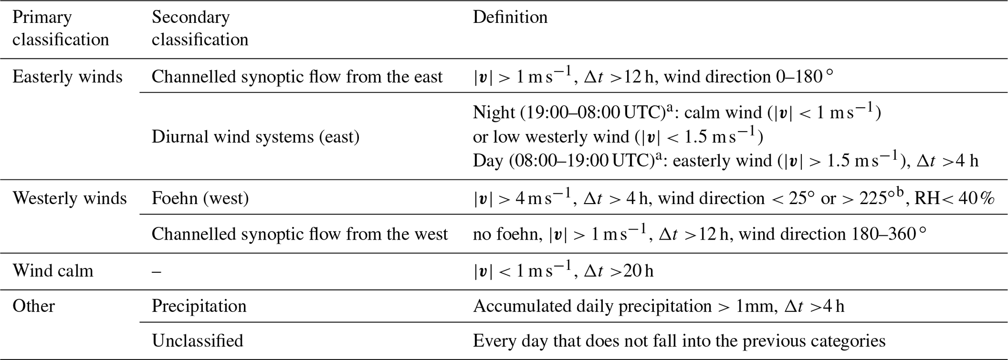
a Both conditions must be met in order to discriminate such diurnal wind systems (inactive at night) from synoptic winds. b The directional range for the foehn cases was determined experimentally by comparison with manual classification from a trained weather observer.
The ALC classification described above was used to derive the seasonal frequency distribution of each aerosol advection class. Relevant results are shown in Fig. 3. Days not falling into those classes (e.g. complex-shaped layers, presence of low clouds or heavy rain hiding the aerosol layer) or including other kinds of aerosol layers (e.g. Saharan dust) were flagged as “Other” and were not considered for further analyses (this accounting for a maximum 26 % of days, in summer). The results reveal that clearly detected aerosol advections (cases C to F) occur half (50 %) of the days in summer and autumn and with a slightly lower frequency (45 %) in winter and spring. A higher percentage of clear days (A) occurs in winter and spring; persistent layers (F) are mostly found in winter, while cases E are more frequent in summer.
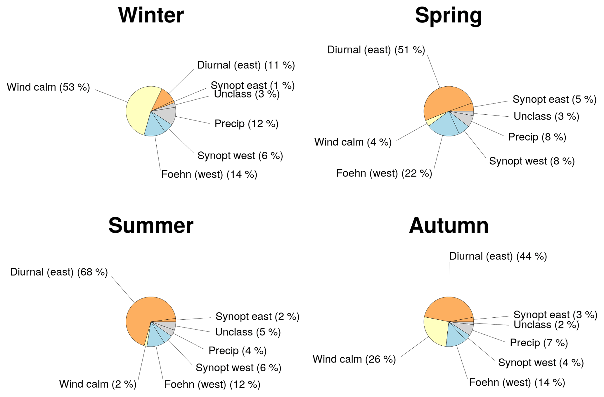
Figure 4Frequency distribution of circulation conditions in Aosta–Saint-Christophe based on the meteorological classification described in Table 2. Easterly winds (diurnal wind systems and channelled synoptic flow from the east) are represented as orange slices, wind calm conditions in yellow, and westerly winds (foehn and channelled synoptic flow from the west) in blue. Precipitation and unclassified days are represented as grey slices and are not used further in the study.
To assess how the ALC classification described above is related to the circulation patterns, we used the surface meteorological observations in Aosta–Saint-Christophe as drivers of a second, independent classification scheme as summarised in Table 2. Seasonal frequency distributions from this meteo-based scheme are displayed in Fig. 4. These show that weather circulation types are remarkably variable during the year and help in interpreting the ALC-based results (Fig. 3). In fact, winter is mostly characterised by wind calm (53 % of the days), which sometimes favours stagnation and persistent aerosol layers (F). Plain-to-mountain diurnal winds gradually increase from winter (only 11 % of the days in that season, which reflects the highest percentage of clear days (A)) to summer (68 % of the days), when the thermally driven regional circulation represents the main mechanism contributing to transport of polluted air masses (E). Foehn winds are fundamental processes, especially in spring (22 % of the days), leading to the removal of pollutants and frequent occurrence of clear days (A) in that season. Finally, channelled synoptic flows from the east (or from the west) are also partly responsible for pushing polluted air masses towards (or away from) the Aosta Valley, although they are markedly less frequent compared to the thermal winds mechanism.
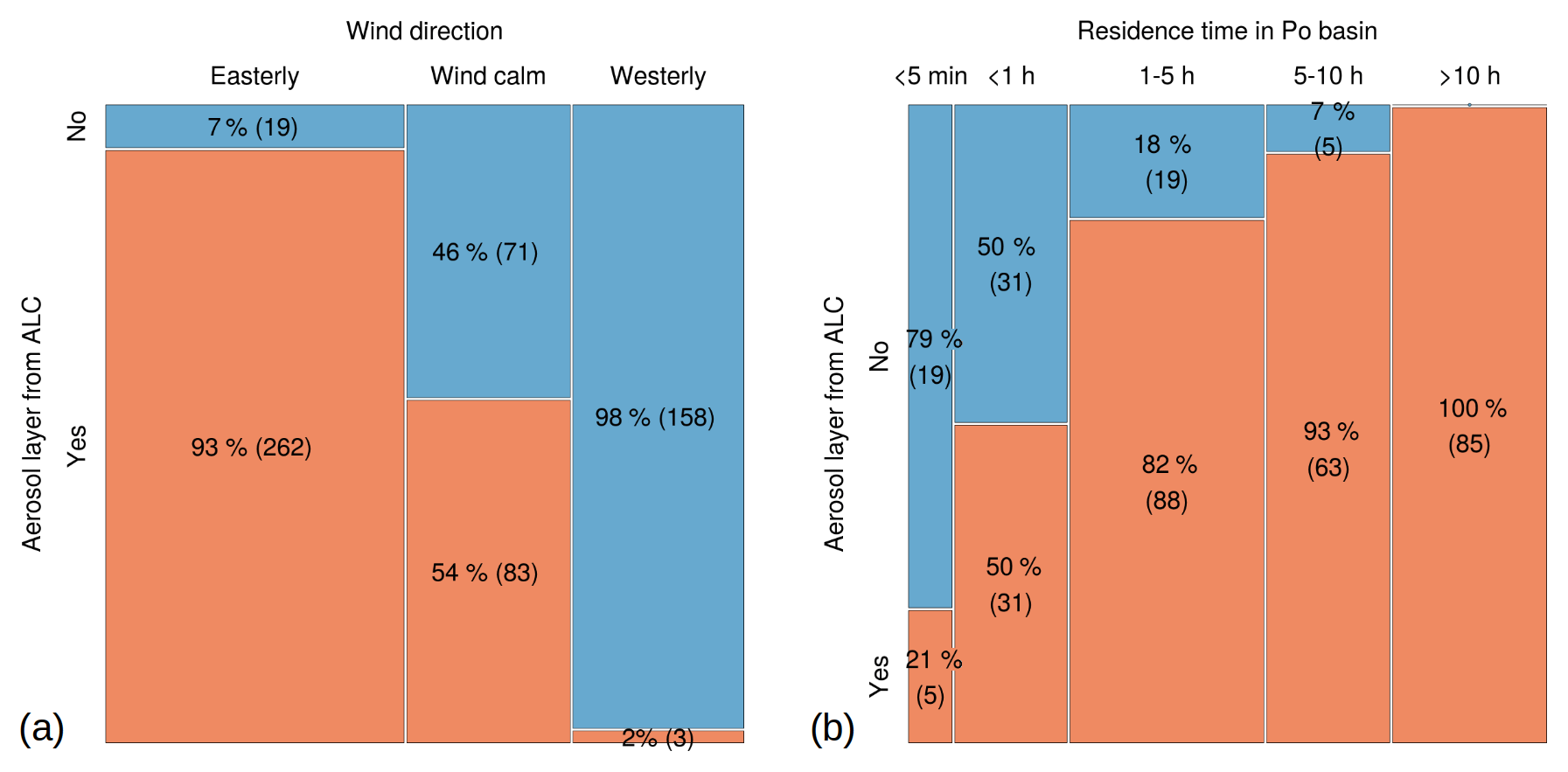
Figure 5(a) Contingency table showing occurrences of the aerosol layer seen by the ALC and wind direction. The blue boxes represent cases when the aerosol layer is not visible (day types A) and pink boxes cases when an arriving or stationary aerosol layer is revealed by the ALC (day types C, E, and F). The numbers inside the boxes refer to the frequency and the number of occurrences for each couple of wind–layer classes. (b) Occurrence of the aerosol layer seen by the ALC and residence time of 48 h back-trajectories in the Po plain.
The association between the ALC- and meteo-based classification schemes was explored using contingency tables (Fig. 5a). To this aim, the ALC classification (A–F) was further simplified and reduced to two main cases: presence of an arriving or stationary aerosol layer (classes C, E, and F) and absence of any thick aerosol layer (class A). Classes B (short and uncertain episodes) and D (layer leaving during the morning) were not used for the next considerations to avoid confounding conditions. Figure 5a shows that the presence of a thick aerosol layer is strongly connected to the wind direction, as expected. In fact, this scheme reveals that the layer appearance can be easily explained using the wind direction as the only information: when air masses come from the east, the probability of detecting an aerosol layer over the Aosta Valley is 93 %, confirming the Po basin as a heavy aerosol source for the neighbouring regions, independently of the day and period of the year. Conversely, this probability reduces to only 2 % of the cases when the wind blows from the west. In the period addressed, we thus detected few exceptions to the perfect correspondence (100 % and 0 %), which can however still be explained. For cases of easterly winds and no aerosol layer found (7 %), possible reasons are
-
the diurnal wind, although clearly detected by the surface network, was of too short a duration or too weak to transport the polluted air masses from the Po basin to Aosta–Saint-Christophe (at least ∼40 km must be travelled by the air masses along the main valley). In our record, this was for example the case of 14 and 18 September 2015, and 17 June 2016;
-
back-trajectories were indeed channelled along the central valley; however, they did not come from the Po basin, but rather from the other side of the Alps. This was the case, for instance, of 20 August 2015, in which air masses came from the Divedro Valley (northeast of the Aosta Valley) after crossing the Simplon pass (between Switzerland and Italy).
These exceptions also help understand why, in summer, about 70 % of the days feature breeze systems (Fig. 4), while aerosol layers are detected on only about 50 % of the days (Fig. 3). Indeed, some part (7 %, Fig. 5a) of this 20 % discrepancy can be attributed to the above events, the remaining 13 % being likely associated with days with a complex aerosol structure (not classified in Fig. 2) or with days affected by low clouds and/or desert dust events. These days were therefore labelled as “Other” in Fig. 3.
There are few cases (2 %, Fig. 5a) in our record in which, conversely, an aerosol layer was associated with westerly, rather than easterly, winds. These are as follows:
-
on 5 February and 15 March 2016, the prevalent wind was from the west and the days were correctly identified as “`Channelled synoptic flow from the west” and “Foehn” respectively. However, as soon as the wind turned and the valley–mountain diurnal circulation started, the aerosol layer arrived;
-
on 24 March 2016, a real case of transboundary/transalpine advection occurred and an aerosol-rich air mass was transported from the polluted French valleys on the other side of the Mont Blanc chain to the Aosta Valley. Although heavy pollution episodes can occur also on the French side of the Alps (e.g. Chazette et al., 2005; Brulfert et al., 2006; Bonvalot et al., 2016; Chemel et al., 2016; Largeron and Staquet, 2016; Sabatier et al., 2018), it is very rare to clearly spot an aerosol layer transported from that region to Aosta, since in those cases air masses coming from the west must have crossed the Alps and are almost always mixed with clean air from the uppermost layers; therefore, only a dim aerosol backscatter signal is usually noticed from the ALC.
Overall, the good correspondence between the measured wind regimes and the aerosol layer detection by the ALC (Fig. 5a) suggests that the same association could be employed to forecast the arrival of an advected aerosol layer based on the predicted wind fields. As an example of the simple forecasting capabilities of this phenomenon, Fig. 5b illustrates a contingency table relating the occurrence of an aerosol layer in Aosta–Saint-Christophe to the residence time over the Po Valley of the 48 h back-trajectories arriving at the Aosta–Saint-Christophe observing site. Again, a direct, clear connection between both variables can be seen, with a 100 % correspondence for residence times of air masses over the Po basin >10 h.
Finally, it is worth mentioning that the proven high correlation between the circulation patterns (observed and/or simulated) and the presence of advected polluted layers in the Aosta area may be exploited in the future to reconstruct the impacts of aerosol transport on air quality over the Alpine region back to previous periods not covered by the ALC measurements (a 40-year long meteorological database is available in the region).
4.2 Vertical and temporal characteristics of the advected aerosol layer
The 2015–2017 ALC time series in Aosta–Saint-Christophe is summarised in Fig. 6, showing the 1 h resolved monthly average SR daily evolution. A data screening was preliminarily performed by removing cloud periods with less than 30 min measurements per hour and points <1 week of measurements per month. The plot clearly shows that the maximum aerosol backscatter is generally found in the early morning and in the late afternoon, likely due to coupling between aerosol transport and hygroscopic effects (Diémoz et al., 2019), and not, as usual for plain sites, in correspondence to the midday development of the mixing boundary layer. Also, the altitude of the layer varies with season. Incidentally, months affected by exceptional events can be sharply distinguished: the frequent Saharan dust events in June and August 2017 and the forest fire plumes from Piedmont in October 2017, the latter again affecting the Aosta site in the afternoon because of the thermally driven circulation. A similar climatology, showing the results in terms of average PM concentration profiles retrieved by the ALC, is given in Fig. S1 of the Supplement. In that case, the conversion from backscatter to PM10 was obtained using the methodology described by Dionisi et al. (2018).
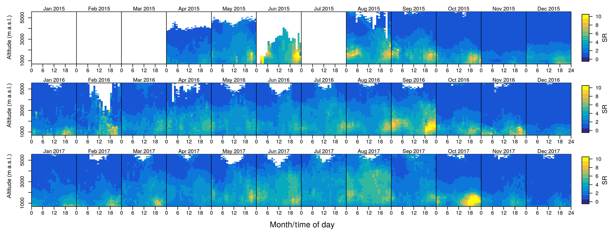
Figure 6Monthly averages of the SR daily evolution (hourly measurements, from 00:00 to 24:00 UTC) from the ALC in Aosta–Saint-Christophe (2015–2017). Although ALC measurements extend up to 15 km altitude, we limited the figure to 5000 m a.g.l. to better show the lowermost levels, where aerosol transport from the Po basin occurs (Diémoz et al., 2019). Points with insufficient statistics are not plotted (white areas; cf. main text).
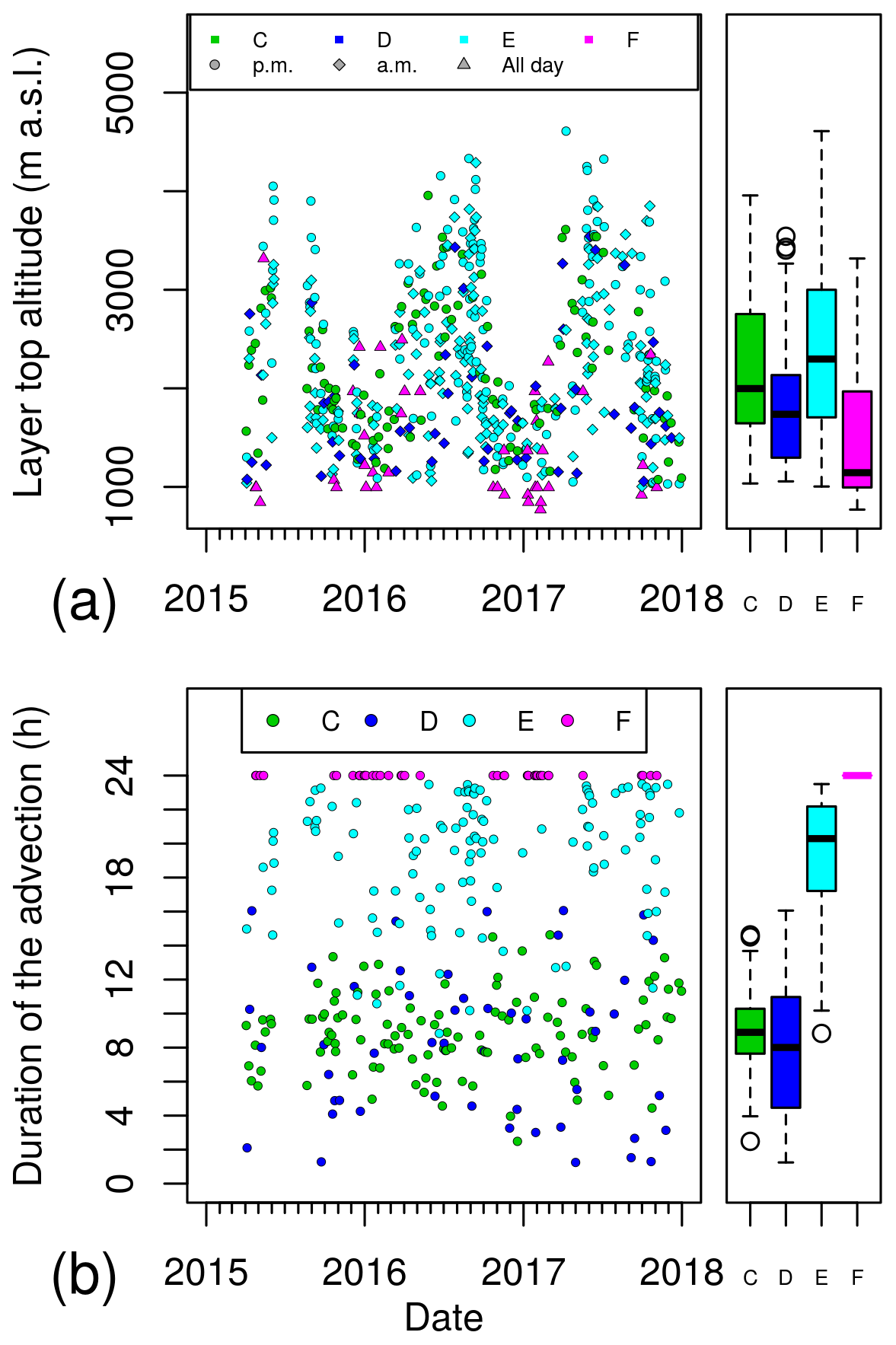
Figure 7(a) Aerosol layer top altitude for the classified days. Marker colour represents the type of the advection, while the marker shape represents the time of the day: morning (a.m.), afternoon (p.m.), or all day (applicable to cases F only). (b) Overall duration of the aerosol layer in a day (morning and afternoon durations were summed up in case E). The boxplots on the right represent synthetic information for each day type (same y scale as the relative charts on the left). Missing measurements in summer 2015 are due to the replacement of the ALC laser module.
To quantitatively explore the spatial and temporal characteristics of the ALC-detected aerosol layer over the long term, we developed an automated procedure, described in detail in the Supplement (Sect. S2), to identify and fit with a sigmoid curve the space–time region of the ALC profiles affected by the aerosol advection (using SR ≥3 as a threshold value). This allowed us to objectively determine, for example, the height and the duration of these advections. The long-term statistics of these two variables is summarised in Fig. 7. The altitude of the polluted aerosol layer (Fig. 7a) displays, as expected, a clear seasonal cycle, with minimum in winter and maximum, up to 4000 m a.g.l., in summer. The overall cycle mimics the variability of the convective boundary layer (CBL) height found in the Po basin by other studies (Barnaba et al., 2010; Decesari et al., 2014; Arvani et al., 2016), with somewhat higher values that reflect the modification of the boundary layer structure in mountainous areas (De Wekker and Kossmann, 2015; Serafin et al., 2018). Notably, stronger, multi-scale thermally driven flows (e.g. the ones developing on the slopes of the valley) further redistribute the aerosol particles in the vertical direction, thus pushing the upper limit of the CBL to the ridge height. Average values of the different classes, represented as boxplots in Fig. 7, are clearly impacted by the season of their maximum frequency over the year (Fig. 3). In fact, minimum altitude of the layer top was found on days F owing to their maximum occurrence in winter, while the top altitude maximum was found on days E being these mostly summertime events. Great variability was also found for the duration of the advection (Fig. 7b), ranging from a few hours in the weakest events to 24 h per day in the extreme cases (full day, by definition, for cases F). The coupling between the duration of the events and their absolute aerosol load determines the impact of the investigated phenomenon on surface air quality, as discussed in the following paragraphs.
4.3 Impact of Po Valley advections on northwestern Alps surface-level PM loads and physico-chemical characteristics
To quantify the impact of the aerosol layers detected by the ALC on the air quality at ground level, we first investigated how the PM concentration daily evolution measured by the surface network changes depending on the ALC-identified classes (Sect. 4.3.1). We then used the positive matrix factorisation of the multivariate dataset of chemical analyses to explore the chemical markers associated with the transport from the Po basin (Sect. 4.3.2). The effectiveness of the identified markers and the coupling between chemistry and meteorology were also confirmed by the use of trajectory statistical models. Furthermore, a link between aerosol chemical and physical properties was investigated in Sect. 4.3.3, where particle chemical composition is coupled to measurements of aerosol particle size. Finally, a preliminary assessment of the effect of the investigated advections on surface pollutants other than particulate matter (e.g. NOx partitioning) was also performed and is reported in the Supplement (Sect. S5).
4.3.1 Surface PM variability in relation to the ALC profiles' classification scheme
We started investigating the effect of aerosol transport on the Aosta Valley surface air quality by analysing the variations of the daily mean PM concentrations measured by the ARPA surface network as a function of the ALC classes introduced in Sect. 4.1. Figure 8a shows the relevant results, resolved by season. It is quite evident that PM10 concentrations in Aosta–Downtown are in fact highly correlated with the presence/strength of the aerosol layers seen by the ALC. PM10 on days with a persistent aerosol layer (class F) was found to be 2 to 3.5 times higher, on average, than on non-event days (class A, this difference being statistically significant for all seasons, as proven by the p value <0.05 from the Mann and Whitney, 1947, test). Similar behaviour was seen in PM2.5 concentrations measured at the same station (Fig. S2a) and in the PM2.5∕PM10 ratio (Fig. S2b), the latter indicating that aerosol particles are smaller, on average, on days when the ALC detects a thick aerosol layer compared to non-event days. Causality between the presence of an elevated layer and variations of the PM surface concentration, however, cannot be rigorously inferred at this point, since, in principle, common environmental conditions affecting both PM at the ground and the aerosol in the layers aloft could generate the observed correlation. Nevertheless, it is interesting to note that this effect is less detectable for other pollutants measured by the network. In fact, concentrations of typical locally produced pollutants such as NOx and PAHs (Fig. 8b and c) do not change as much as PM among the ALC classes, with only rare exceptions (e.g. class A, which is slightly influenced by foehn winds, and class F, in which temperature inversions/low mixing layer heights may enhance the effect of local surface emissions). These results indicate that the correlation (Fig. 8a) does not trivially originate from common weather conditions or from the uneven distribution of the ALC classes among the seasons.
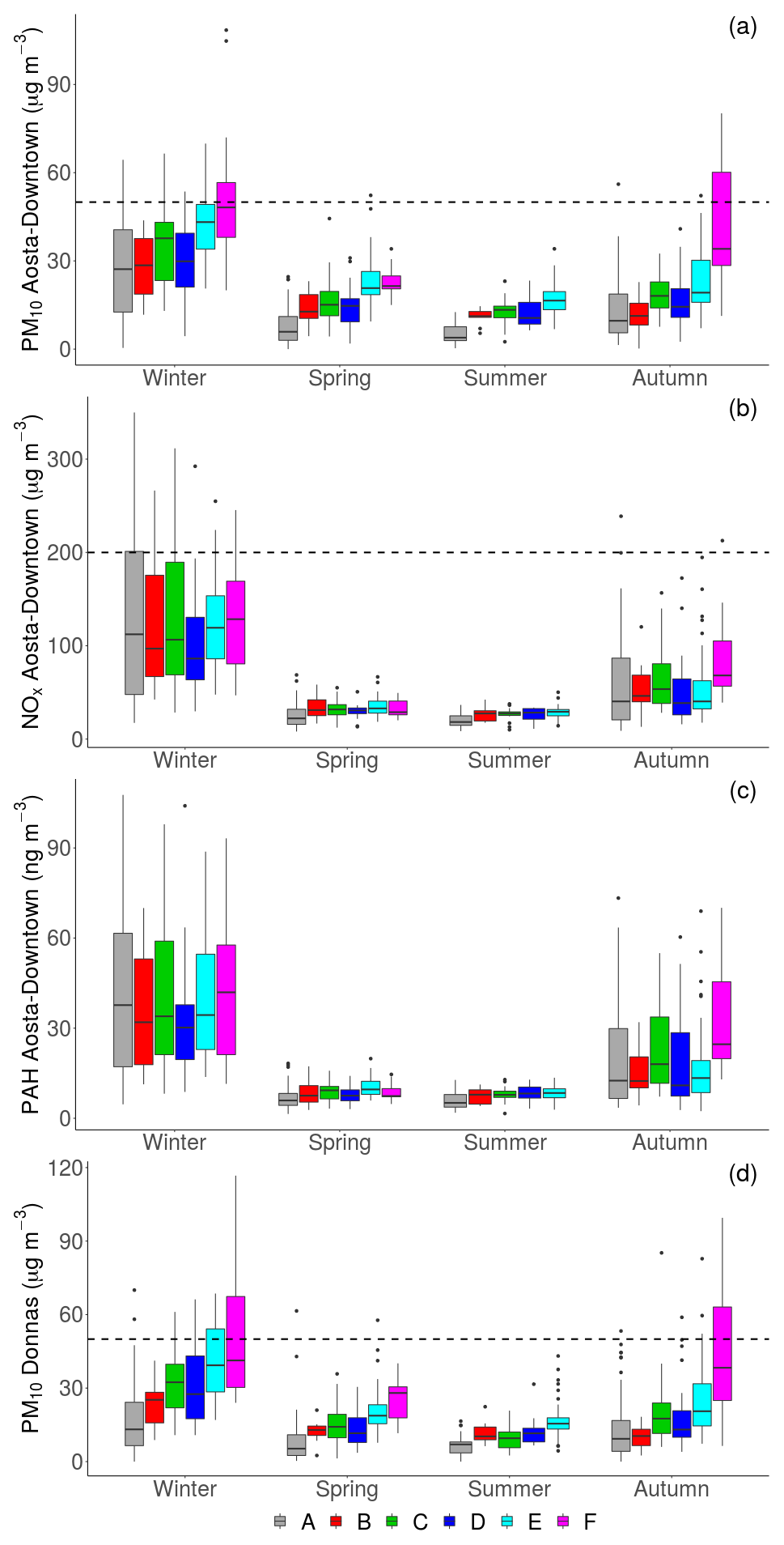
Figure 8Daily averaged surface concentrations (2015–2017) of PM10 (a), nitrogen oxides (b), and polycyclic aromatic hydrocarbons (c) in Aosta–Downtown as a function of the ALC classes and season. (d) PM10 surface concentration at the Donnas station. The EU-established PM10 daily limit of 50 µg m−3 and the NO2 hourly limit of 200 µg m−3 are also drawn as references (horizontal dashed lines).
Furthermore, large correlation was also found between the ALC classification only available in Aosta–Saint-Christophe and the surface PM10 concentration recorded in Donnas (Fig. 8d). Since the two stations are located at 40 km distance, this result suggests that a major role is played by large-scale dynamics rather than by local sources and that the phenomena under consideration have at least a regional-scale extent. As a further test, we correlated the daily PM10 concentrations measured in Donnas with those measured in Aosta. To this purpose, we considered the anomaly (ΔPM10, Eq. 5) with respect to the monthly moving average (〈PM10〉m), in order to avoid large, fictitious correlations due to the same yearly cycle (maximum PM concentration in winter and minimum in summer), and only focus on the short-term dynamics:
where t is a specific day. The scatterplot of these anomalies is shown in Fig. 9. It highlights the good correlation between the ΔPM10 at the two sites (ρ=0.73 when considering all classes and ρ=0.76 when only considering advection cases, i.e. classes C to F). Clustering of these results using the ALC classification (circle colours) further shows the different ΔPM10 associated with the different classes and the good correspondence of this effect at both sites. Notably, in the most severe cases (E and F), the anomalies in Donnas are generally larger than in Aosta–Downtown (the best fit line being for cases E and F only), which is compatible with this site being closer to the Po basin (Fig. 1).
The advected aerosol layers were also found to impact the daily evolution of surface PM concentrations. To investigate this aspect, we used hourly and sub-hourly PM10 data from both the Fidas 200s OPC in Aosta–Saint-Christophe and the TEOM in Aosta–Downtown. Figure 10 shows the PM10 daily cycles for cases A (no advection), C, and D, for both Aosta–Saint-Christophe (Fig. 10a) and Aosta–Downtown (Fig. 10b). Despite the instruments' limitations described in Sect. 2, the figure shows that local effects play an important role in the PM10 daily evolution, as visible from the morning and afternoon peaks. In fact, these maxima, common to most pollutants, are the results of the coupled effect of varying local emissions and boundary layer height during the day. The daily cycle of PAH concentrations is added to the plot as a proxy of the diurnal cycle from local sources (dashed line, right y axis). This cycle is similar to the PM10 one for case A. Conversely, the influence of the advections (C and D) is clearly visible in the corresponding PM10 cycles. In fact, Fig. 10 shows the PM10 concentration to markedly increase in the afternoon of days C (by 1.0 and 0.7 µg m−3 h−1 in Aosta–Saint-Christophe and Aosta–Downtown respectively) and to markedly decrease on days D (by −1.3 and −0.7 µg m−3 h−1). This effect is similar at the two sites, although less marked in Aosta–Downtown, especially at night. This is probably due to TEOM loss of volatile species in the advected aerosol (see also the PMF results on chemical analysis in the following section). Similar results (not shown) were obtained when splitting the data on a seasonal basis, which excludes the observed behaviour originating from the seasonal cycle.
4.3.2 Chemical species within the advected aerosol layers
As a further step to adequately discriminate local and non-local sources, we took advantage of the 1-year long (2017) chemical aerosol characterisation dataset in the urban site of Aosta–Downtown and applied the PMF to the three datasets described in Sect. 3.3 (PMF datasets a, b, c, i.e. anion/cation only, anion/cation with EC/OC, and anion/cation with metals respectively). Results of this analysis show the main factors shaping the composition of PM10 at the investigated site are those given in Fig. 11, all details on this outcome being given in Sect. S4. The question addressed here is, however, how aerosol transport from the Po Valley affects the chemical properties of PM10 sampled in Aosta. In the preliminary analysis of three case studies reported in the companion paper, we found that the advected layers were rich in nitrates and sulfates (accounting, together with ammonium, for 30 %–40 % of the total PM10 mass). This kind of secondary inorganic aerosol was indeed found in high concentrations in the Po basin by previous studies (e.g. Putaud et al., 2002, 2010; Carbone et al., 2010; Larsen et al., 2012; Saarikoski et al., 2012; Gilardoni et al., 2014; Curci et al., 2015). Here we further tested on a longer dataset whether the sum of the nitrate- and sulfate-rich factors (i.e. secondary aerosols) could in fact represent a good chemical marker of aerosol transport from the Po basin (e.g. Kukkonen et al., 2008; Tang et al., 2014). In this respect, it is worth highlighting that these PMF modes are not correlated with typical locally produced pollutants such as NOx and PAHs (this is revealed by the low percentage contribution of NOx and PAHs in nitrate-rich and sulfate-rich modes in Figs. S3–S5), which therefore excludes their local origin. We then combined the chemical information (the sum of the secondary components) with the ALC classification. This was done for the year 2017, which is the only overlapping period between anion/cation analyses and ALC profiles (see Table 1). Results are shown in Fig. 12. In particular, Fig. 12a shows the time evolution of the mass concentration carried by the secondary aerosol modes, in which each date is coloured according to the six ALC classes identified. It can be noticed that almost all peak values occur during days of type E or F, i.e. when the advected layer is more persistent and able to strongly influence the local air quality at the ground. The very good correspondence between the sum of the nitrate- and sulfate-rich mode contributions and the ALC classification, as well as the poor correlation between the latter and the role of the other PMF-identified modes (not shown), suggests that the link between the secondary components and the aerosol layer advection is not simply due to particular weather conditions affecting both variables. Rather, the coupling between the chemical and the ALC information indicates that aerosols of secondary origin dominate during the advection episodes from the Po basin.
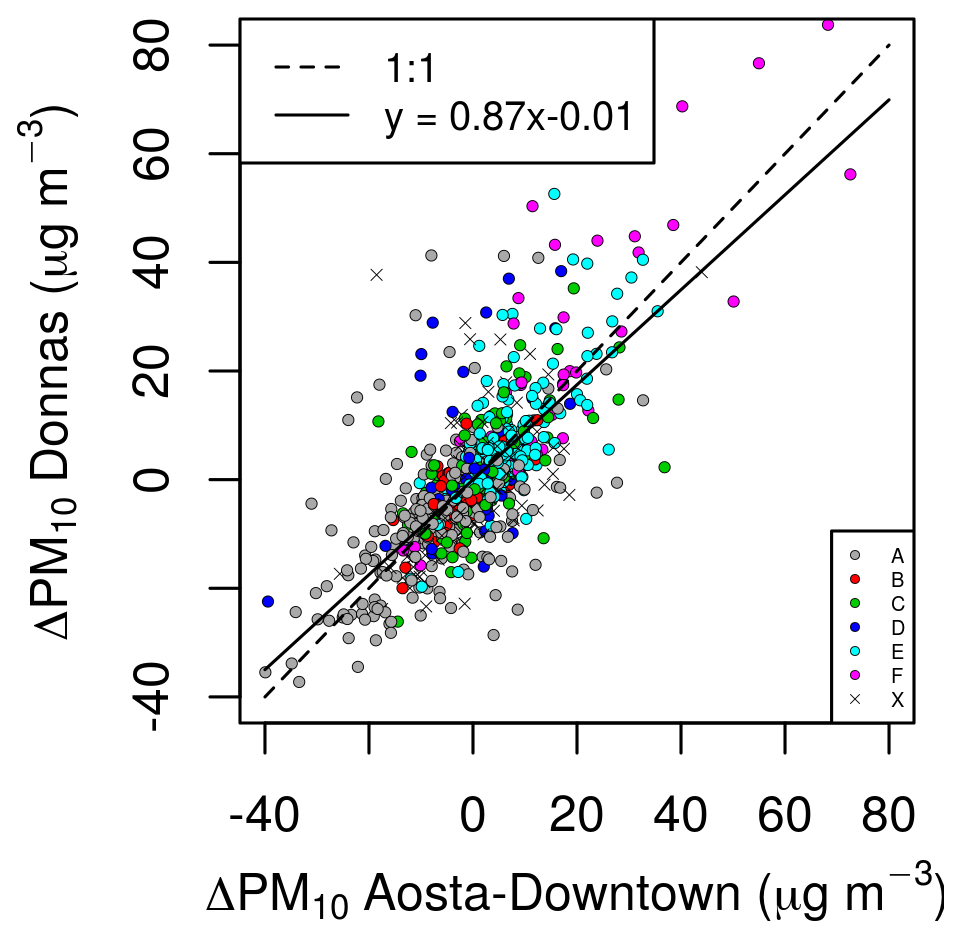
Figure 9Comparison between daily PM10 anomalies (Eq. 5) registered in Aosta–Downtown and Donnas (40 km apart), relative to a monthly moving average. Circle colour represents the ALC classification (see legend), and the “X” symbol represents the unclassified days. The 1:1 and the best fit line are also represented on the plot. Pearson's correlation index between the two series is ρ=0.73.
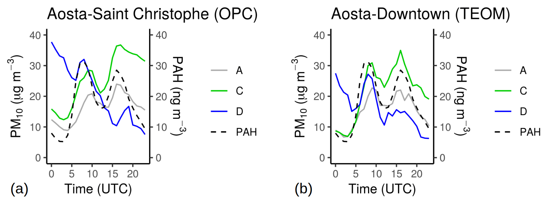
Figure 10(a) Daily PM10 cycle sampled by the OPC in Aosta–Saint-Christophe during non-event days (class A) and days with arriving and leaving aerosol layers (classes C and D), plotted together with the daily evolution of PAH as a proxy of the local sources (dashed line, right vertical axis, in ng m−3). (b) Same as (a) using the TEOM in Aosta–Downtown.
A summary of the contribution of secondary modes to the total PM10 as a function of the day type, on a statistical basis, is given in Fig. 12b. The Mann–Whitney test, applied to these data, confirms that the contribution of secondary pollutants is significantly lower for class A compared to B (p=0.0005, ), C compared to D (), D compared to E (), and E compared to F (). Figure 12b also allows us to quantify the contribution of non-local sources using as a baseline the results obtained for class A (i.e. no advection, shaded area in Fig. 12a). Note that this baseline is very low on average, about 3 µg m−3, as expected from the unfavourable conditions for secondary aerosol production in the area under investigation (e.g. low expected emissions of ammonia, frequent winds) and from the unobserved correlation between secondary aerosol components and their gas-phase precursors. The non-local contribution is calculated as the average difference between the mass from the secondary modes and this baseline, and amounts to about 5 µg m−3 on a yearly basis, i.e. 24 % of the total PM10 concentration reconstructed from the PMF. On a seasonal basis, the absolute impact of air mass transport depends on the coupling between emissions (stronger in winter and weaker in summer) and weather regimes (e.g. thermal winds occurring more frequently in summer/autumn with respect to winter/spring, Sect. 4.1). This results in a PM10 contribution of nearly 6 µg m−3 in winter and autumn, 4 µg m−3 in summer, and 3 µg m−3 in spring. In terms of relative contribution, this also depends on the “background” PM10 levels in Aosta. It is therefore highest in summer (32 %), when thermally driven fluxes are more frequent and local emissions lower, and lowest in winter (16 %), when thermal winds are less frequent and local emissions higher. Intermediate relative values are found in spring and summer (27 % and 28 % respectively). In specific episodes, advections from the Po basin may still produce an increase in PM10 concentrations of up to 50 µg m−3, i.e. exceeding alone the EU daily threshold. The most important compounds contributing to this increase are nitrate, ammonium, and sulfate, i.e. the species characterising the nitrate- and sulfate-rich PMF modes. However, since the sulfate-rich mode additionally includes organic matter (OM; cf. Figs. S3–S5), the latter species is also relevant in the advection episodes, especially in summer, when the nitrate-rich mode has its lowest contribution. This finding agrees with previous works, identifying the Po basin as a source of organic aerosol (Putaud et al., 2002; Matta et al., 2003; Gilardoni et al., 2011; Perrone et al., 2012; Saarikoski et al., 2012; Sandrini et al., 2014; Bressi et al., 2016; Khan et al., 2016; Costabile et al., 2017).
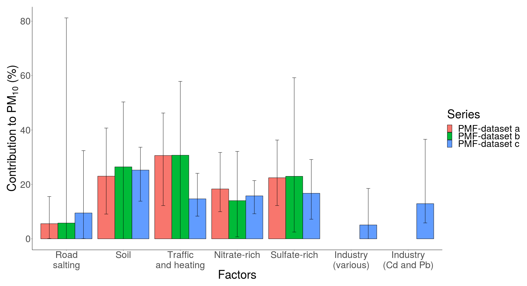
Figure 11Percentage of aerosol mass concentration carried by each mode for the three PMF datasets considered in the analysis (PMF dataset a: anion/cation only; PMF dataset b: anion/cation together with EC/OC; PMF dataset c: anion/cation together with metals) and their respective confidence intervals from the BS-DISP test. Details are provided in Sect. S4.
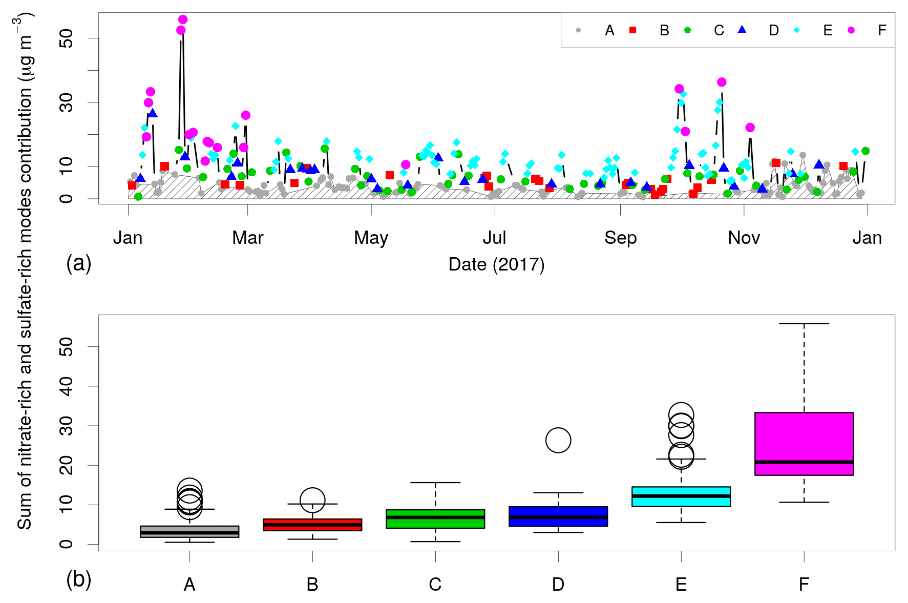
Figure 12(a) Temporal chart of the contribution of secondary (nitrate-rich and sulfate-rich) modes to the total PM10. The shaded area represents the estimated local production of secondary aerosol. The difference between each dot and this baseline can thus be read as the non-local contribution to the aerosol concentration in Aosta–Downtown. Since ion chemical speciation started in 2017, only 1 year of overlap with the ALC is available at the moment (see Table 1). (b) Boxplot of the contribution of secondary (nitrate-rich and sulfate-rich) modes to the total PM10 concentration as a function of the day type. PMF dataset “a” was used for both plots.
The Po Valley origin of the secondary components was also further proved by coupling the chemical information to back-trajectories. Figure 13a shows the result of the TSM using the sum of the nitrate- and sulfate-rich modes as a concentration variable at the receptor. It clearly reveals that trajectories crossing the Po basin have a much higher impact on secondary aerosol measured in Aosta compared to air parcels coming from the northern side of the Alps. Interestingly, this is not the case using different source factors from PMF. For example, Fig. 13b reports the same map, but relative to the traffic and heating mode, which is clearly much more homogeneous compared to Fig. 13a and essentially reflects the density distribution of the trajectories. This behaviour highlights the local origin of the PMF source factors other than the two chosen as proxies of the advection (secondary aerosols). As sensitivity tests, similar maps, without any weighting applied, are reported in Fig. S7. No substantial differences can be noticed.
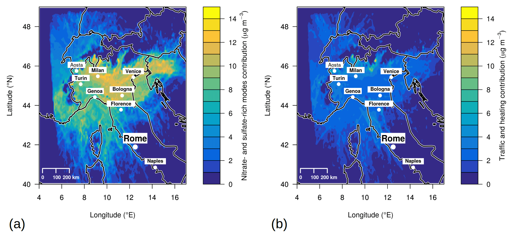
Figure 13(a) Output of the Concentration Field Trajectory Statistical Model, using the sum of the contributions from PMF nitrate- and sulfate-rich modes as a concentration variable at the receptor (Aosta–Downtown). (b) Concentration field based on the traffic and heating mode from PMF. Trajectories are cut at the borders of the COSMO-I2 domain.
4.3.3 PMF of aerosol size distributions and links to chemical properties
Exploring the links between aerosol chemical and physical properties is useful to get insights into the atmospheric mechanisms leading to particle formation and transformation during their transport to the Aosta Valley. Therefore, we investigated correlations between the results of the chemical analyses on samples collected in Aosta–Downtown and particle size distributions (PSDs) measured by the Fidas OPC in Aosta–Saint-Christophe. To ensure comparability between these two datasets, the particle volume distributions from the Fidas OPC (normally extending up to sizes of 18 µm) were weighted by a typical cut-off efficiency of PM10 sampling head (Sect. S6). We then performed a PMF analysis of the hourly averaged PSDs from the Fidas OPC (hereafter referred to as size-PMF). Four principal modes were identified. Their relative contribution to the total particle volume is shown in Fig. 14a. These modes are centred at 0.2, 0.5, 2, and 10 µm diameter respectively and will be thus referred to as 0.2, 0.5, 2, and 10 µm size-PMF modes in the following. A similar figure, showing their dependence on season, wind speed, and direction, is also provided in Fig. S10. The number of factors (p) was chosen based on physical considerations: if p>4, then the last mode (largest sizes) splits into sub-modes, which are not relevant for the present study; conversely, if fewer components (p<4) are retained, they merge into unphysical modes (e.g. very large and very fine particles combined together).
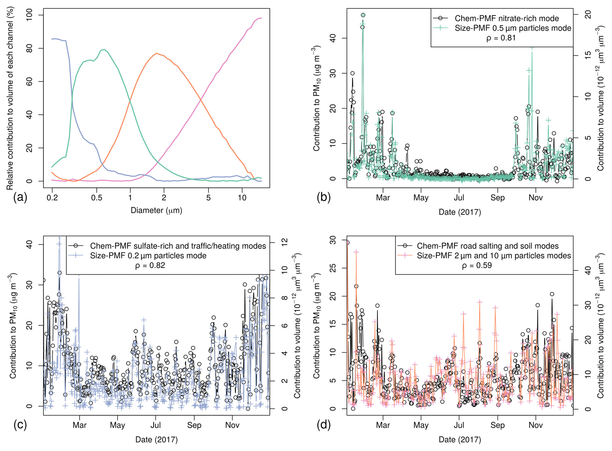
Figure 14(a) Modes identified by the PMF analysis applied on the PSDs measured by the Fidas OPC (size-PMF). (b–d) Comparison between the PMF scores' time series obtained from analysis of chemical speciation (chem-PMF on PMF dataset “a”, showing mass, left-hand vertical axes) and size distributions (size-PMF, showing volume, right-hand vertical axes). The three panels show (b) contributions from chem-PMF nitrate-rich (black) and size-PMF 0.5 µm (green) modes; (c) contributions from the sum of the chem-PMF sulfate-rich and traffic and heating modes (black) and from the 0.2 µm size-PMF mode (blue); (d) sum of contributions from chem-PMF road salting and soil modes (black) and from 2 and 10 µm size-PMF modes (red). Correlation values (ρ) are also reported in each plot.
The scores from the size-PMF were then averaged on a daily basis to be compared to the chemical PMF ones (hereafter, chem-PMF; Sect. S4). Figure 14 compares time series of selected chem-PMF (dataset a) and size-PMF results. It shows that
- a.
the nitrate-rich mode from chem-PMF and the 0.5 µm size-PMF mode correlate very strongly (ρ=0.81, Fig. 14b);
- b.
the sum of the sulfate-rich mode and traffic and heating mode correlates very strongly with the 0.2 µm size-PMF mode (ρ=0.82, Fig. 14c). Note that the correlation index decreases (ρ between 0.35 and 0.69) if the sulfate-rich mode and traffic and heating mode are compared separately with the 0.2 µm mode;
- c.
a moderate, statistically significant correlation was found between the chem-PMF soil plus road salting modes and the size-PMF coarser modes (sum of 2 and 10 µm modes, Pearson's correlation index ρ=0.59, p value , Fig. 14d). This suggests that both indicate the same source, and likely non-exhaust traffic emissions, such as abrasion from brakes, tire wear, and road (with typical sizes of 2–5 µm), and resuspension from the surface (up to >10 µm), as also found in other studies (e.g. Harrison et al., 2012). This agreement between the two independent datasets is remarkable considering that the particles were sampled at two different sites (Aosta–Saint-Christophe and Aosta–Downtown) with distinct environmental features, and that coarse particles usually travel for short ranges. It is also worth mentioning that the correlation between single modes from chem-PMF (road salting or soil) and size-PMF (2 or 10 µm) separately is weaker (ρ between 0.26 and 0.55) than the one resulting from their sum. Finally, from a preliminary analysis based on back-trajectories and desert dust forecasts (NMMB/BSC-Dust, http://ess.bsc.es/bsc-dust-daily-forecast, last access: 2 August 2019), the 2 µm component seems to be additionally connected to deposition, and possibly resuspension, of mineral Saharan dust in Aosta, an effect already observed in other urban areas in central Italy (Barnaba et al., 2017).
A further interesting feature is the clear size separation of the 0.2 and 0.5 µm accumulation modes, which likely results from different aerosol formation mechanisms in the atmosphere: condensation/coagulation from primary emissions/aging on the one hand (0.2 µm mode, also known as “condensation mode”) and aqueous-phase processes (e.g. in fog during the cold season) on the other hand (forming “droplet mode” aerosol particles of about 0.5 µm diameter, e.g. Seinfeld and Pandis, 2006; Wang et al., 2012; Costabile et al., 2017). Finally, the very good correlation between the fine particles and the nitrate- and sulfate-rich modes at the two stations is a further hint that these kinds of particles are mostly of non-local origin.
Overall, the good agreement between the size- and chem-PMF results further strengthens their independent outputs.
4.4 Impact of Po Valley advections on northwestern Alps columnar aerosol properties
ALC measurements revealed the vertical extent and thickness of the advected polluted layers from the Po Valley. We therefore also investigated whether and how much these layers impact the column-integrated aerosol properties (i.e. those sounded by ground-based Sun photometers, but also by satellites). To this purpose, the ALC day-type classification was applied to the measurements of the Aosta–Saint-Christophe Sun photometer. The average AOD at 500 nm, binned by day type and season, is shown in Fig. 15a. It can be noticed that a general increase in the AOD is found from classes A (about 0.04 on average) to F, for which AOD is more than 4 times higher (0.18). The advections are also found to affect the Ångström exponent (Eq. 2, Fig. 15b), representative of the mean particle size. Results from this column-integrated perspective confirm that the transported particles are on average smaller than the locally produced ones. In fact, the mean Ångström exponents vary from 1.0 for days A in winter and autumn up to 1.6 for days E–F, and show a general increase among the classes for every season. To confirm and fully understand this dependence of the Ångström exponents on the ALC classification, we also investigated the columnar volume PSDs retrieved from the Sun photometer almucantar scans during the Po Valley pollution transport events. This analysis (Fig. S11) confirms what we already found with the surface-level PSDs from the Fidas OPC, i.e. that the advections increase the number of particles in all sizes, notably in the sub-micron fraction. This explains the higher Ångström exponents retrieved by the Sun photometer during the advections.
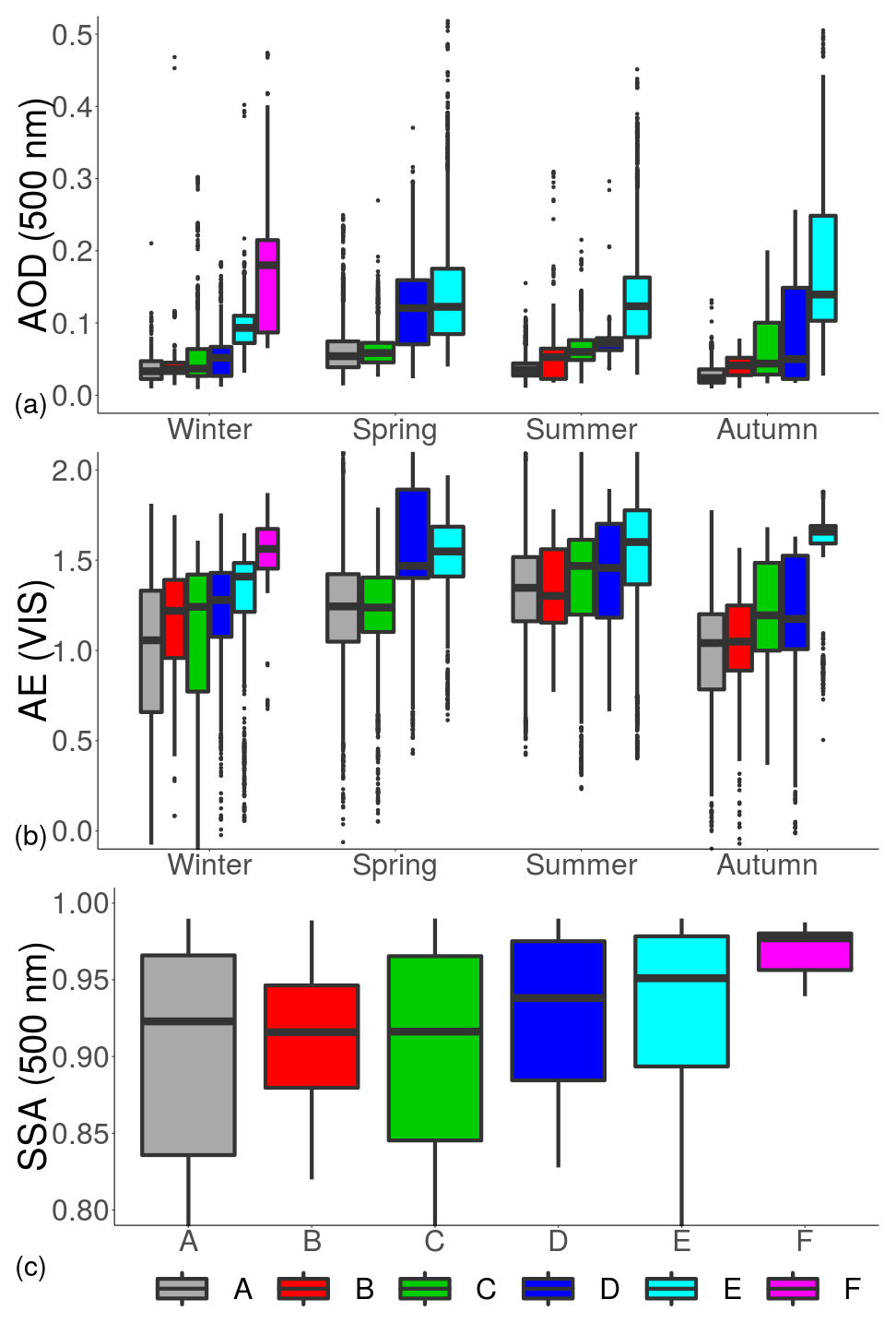
Figure 15(a) Average aerosol optical depth at 500 nm from the POM Sun photometer for each day type (colour code as in Fig. 12) and season; (b) Ångström exponent calculated in the 400–870 nm band; (c) yearly averaged single scattering albedo at 500 nm. B days in spring were removed from panels (a) and (b) due to insufficient statistics (only 3 d).
A further link between aerosol physical and chemical properties is explored through the variability of the single scattering albedo with day type (Fig. 15c). Yearly averaged data are shown in this case due to the limited number of data points available for this parameter (the almucantar plane must be free of clouds to accurately retrieve the SSA, Sect. 2). Figure 15c reveals that SSA at 500 nm generally increases from class A to class F (0.92 to 0.98), which agrees with the fact that secondary, and thus more scattering, aerosol is transported with the advections. This information is particularly important for follow-up radiative transfer evaluations under the investigated conditions. In this respect, also note that further analysis more focussed on the impact of these advections on particle absorption properties is planned for the future.
4.5 Comparison between observations and CTM simulations
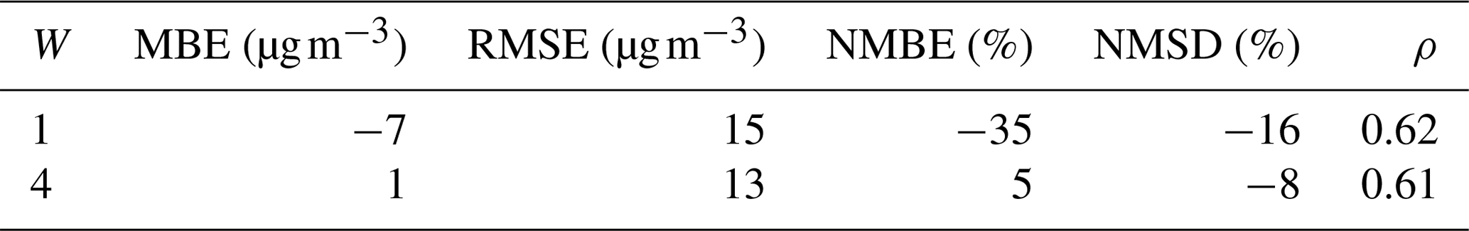
Accurate simulations of air-quality metrics are of utmost importance for environmental protection agencies. Indeed, not only are they essential from a scientific/technical perspective (contributing to better understanding the local and remote pollution dynamics), but they also represent a fundamental duty towards the public, air-quality forecasts being disseminated every day. In this section, we compare long-term (1-year, 2017) daily averages of surface PM10 to the corresponding simulations by FARM in Aosta–Downtown (similar results are found for the other sites in the domain and are not reported here) and next to Ivrea. This exercise was also aimed at evaluating whether and how the information gathered by the ALC can be used to understand deficiencies and thus improve the model performances. The 1-year time series of both the measured and simulated PM10 in the Aosta–Downtown and Ivrea sites are displayed in Fig. 16. Model and measurement show similarities (such as the same seasonal cycle, indicating that local emissions from the regional inventory and general atmospheric processes are correctly reproduced), but also divergences (especially PM10 underestimation by FARM, as already shown and discussed in the companion paper). Table 3 summarises some statistical indicators of the model–measurement comparison, namely mean bias error (MBE), root mean square error (RMSE), normalised mean bias error (NMBE), normalised mean standard deviation (NMSD, i.e. , where σM and σO are the standard deviations of the model and observation), and Pearson's correlation coefficient (ρ). The overall performances of FARM are comparable to the results obtained in other studies using CTMs (e.g. Thunis et al., 2012). For the Aosta–Downtown case, we additionally explore the absolute (Fig. 17a) and relative (Fig. 17b) differences between modelled and observed PM10 in relation to the ALC-derived classes. These results reveal that the model underestimation mostly occurs in the cases of strongest advections (F), with extreme model deviations as low as −40 µg m−3 (Fig. 17a), i.e. −50 % or lower (Fig. 17b). The observed model–measurement discrepancies might originate from (1) an incomplete representation of the inventory sources (emission component), (2) inaccurate NWP modelling of the meteorological fields, and notably the wind (transport component), or a combination of (1) and (2). Some details on these aspects are provided in the following.
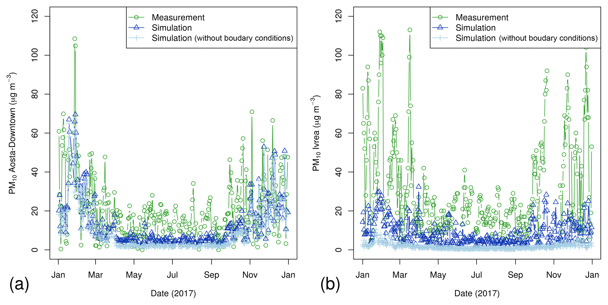
Figure 16Long-term (1-year) comparison between PM10 surface measurements and simulations (FARM) in Aosta–Downtown (a) and Ivrea (b).
Table 3Statistics of comparison between PM10 model forecasts and measurements at the site of Aosta–Downtown. Results with both W=1 and W=4 weighting factors of the PM fraction arriving from outside the boundaries of the regional domain are reported.
-
Emissions. Inaccuracies in the (local and national) emission inventories could degrade the comparison between simulations and observations. Based on results shown in Fig. 17a, b, we decided to investigate the sensitivity of our simulations in Aosta–Downtown to the magnitude of the external contributions (boundary conditions). In particular, we used a simplified approach to speed up the calculations: assuming that the contribution from outside the regional domain and the local emissions add up without interacting, we simulated the surface PM10 concentrations turning on/off the boundary conditions (dark- and light-blue lines in Fig. 16) to roughly estimate the only contribution from sources outside the regional domain. Interestingly, the difference between the two FARM runs correlates well with the advection classes observed by the ALC (Fig. 18). This clear correlation between the simulations and the experimentally determined atmospheric conditions is a first good indication that the NWP model used as input to the CTM yields reasonable meteorological inputs to FARM. Then, to further explore the sensitivity to the boundary conditions, we gradually increased, by a weighting factor W, the PM10 concentration from outside the boundaries of the domain trying to match the observed values. In Fig. 17c, d we show the results obtained with W=4. This exercise shows that the overall mean bias error is much reduced compared to the original simulations (W=1, Fig. 17a, b), especially for the winter and autumn seasons, while slight overestimations are now visible for summer and spring. Also, the annually averaged MBE, NMBE, and NMSD improve (Table 3), whilst the other statistical indicators remain stable or even slightly worsen.
Clearly, our simplified test has major limitations. For example, seasonally and geographically dependent (i.e. relative to the position on the regional domain border) factors W should be used to better correct deficiencies in the national inventory. Also, the high weighting factors needed to match the measurements in winter and autumn suggest not only underestimated emissions, but also missing aerosol production mechanisms (e.g. aqueous-phase particle production as in fog/cloud processing, Gilardoni et al., 2016) during the cold season. In fact, this simplified exercise was only intended to roughly estimate the magnitude of the “outside PM10 tuning factor” necessary to match the observations. Despite this limitation, this numerical experiment still shows quite convincingly that biases in air-quality forecasts can be reduced by revising the emission inventories on the basis of experimental data, among them those from unconventional air-quality systems (e.g. the ALCs used in this study).
-
Transport. Although the COSMO-I2 grid spacing is certainly in line with that of other state-of-the-art operational limited-area models, in our complex terrain it could be insufficient to appropriately resolve local meteorological phenomena triggered by the valley orography (Wagner et al., 2014b), also considering that the actual model resolution is 6–8 times that of the grid cell (Skamarock, 2004). For example, Schmidli et al. (2018) show that at a 2.2 km grid step the COSMO model poorly simulates valley winds, while at a 1.1 km grid step the diurnal cycle of the valley winds is well represented. Similarly, Giovannini et al. (2014) show that a 2 km step can be considered the limit for a good representation of valley winds in narrow Alpine valleys. The smoothed digital elevation model (DEM) used within COSMO and FARM could also play a direct role in the detected underestimation. In fact, as mentioned in Sect. 3.2, the model surface altitude of the Aosta urban area is 900 m a.s.l., whereas the actual altitude is about 580 m a.s.l. (Table 1). The adjacent cells are given an even higher altitude, owing to the fact that the valley floor and the neighbouring mountain slopes are not properly resolved at the current resolution. This results in an apparent lower elevation of the sites located in flatter and wider areas, such as Aosta, while the real topography profile at the bottom of the valley presents a monotonic increase from the Po plain to Aosta. Therefore, it is expected that, just by better reproducing the orography, a higher resolution would better resolve the horizontal advection of aerosol-laden air from much lower altitudes on the plain.
Most of these issues were extensively addressed in the companion paper (Diémoz et al., 2019). In that study, COSMO-I2 was shown to be capable of reproducing the mountain–plain wind patterns observed at the surface, both on average (cf. Fig. S1 in the companion paper) and in specific case studies (Fig. S13 therein). Nevertheless, it was also found to slightly anticipate in time and overestimate the easterly diurnal winds in the first hours of the afternoon and to overestimate the nighttime drainage winds (katabatic winds, ventilating the urban atmosphere and reducing pollutant loads). These limitations were mostly attributed to the finite resolution of the model.
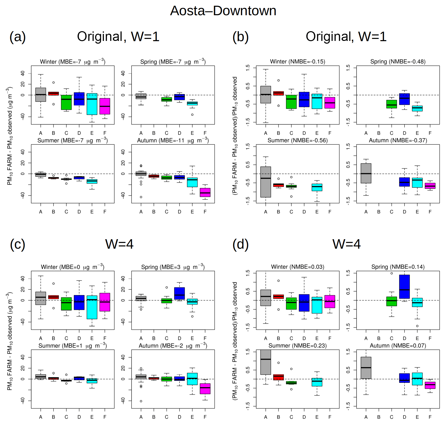
Figure 17Absolute (a, c) and relative (b, d) differences between simulated and observed PM10 concentrations at the surface in Aosta–Downtown. The mean bias error (MBE) and the normalised mean bias error (NMBE) for each case are reported in the plot titles. (a, b) FARM simulations as currently performed by ARPA. (c, d) The PM10 concentrations from outside the boundaries of the domain were multiplied by a factor W=4.
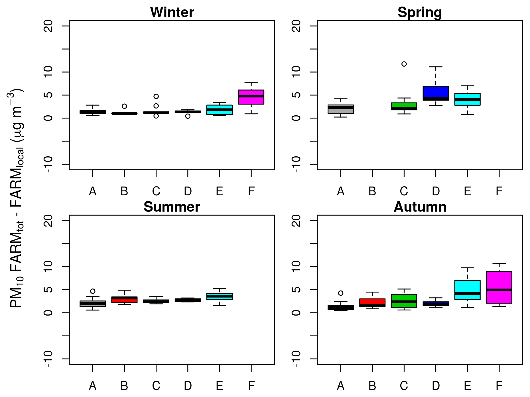
Figure 18Difference between PM10 surface concentrations in Aosta–Downtown simulated by FARM taking the boundary conditions into account (FARMtot) and without taking them into account (FARMlocal, only local sources), as a function of the advection class observed by the ALC.
To disentangle the role of factors (1) and (2) discussed above, we evaluated the model performances in a flatter area of the domain, where simulations are expected to be less affected by the complex orography of the mountains. We therefore compared PM10 simulations and measurements in Ivrea (Fig. 16b). This test is also useful for operating the CTM at the boundaries of the domain, with special focus on the emissions from the “boundary conditions”. Model underestimation in both the warm and cold seasons is evident. Incidentally, it can be noticed that concentrations simulated without “boundary conditions” are nearly zero, since the considered cell is far from the strongest local sources and most of the aerosol comes from outside the regional domain. As done for Aosta (Fig. 17a, b), Fig. 19a, b present the absolute and relative differences between the model and the observations in Ivrea. The overall NMBE is −0.73, which rather well corresponds to the underestimation factor W=4 (or NMBE ) found for Aosta–Downtown and other sites in the valley. Since it is expected that in this flat area the NWP model is able to better resolve the circulation compared to the mountain valley, this result suggests poor CTM performances to be mostly related to underestimated emissions at the boundaries rather than to incorrect transport. In addition to this general underestimation, a large scatter between observations and simulations can be noticed in Fig. 16, the linear correlation index between simulations and observation in Ivrea being rather low (ρ=0.54). If such a large scatter, due to the erroneous boundary conditions, is already detectable at the border of the domain, it is likely that at least part of the RMSE reported in Table 3 for Aosta–Downtown can be attributed to inaccuracies in the national inventory. As already mentioned, an additional contribution to the observed RMSE could still be given by errors in modelling transport due to the coarse resolution of the NWP model, although we are not able to quantify the relative role of the two factors. To unravel this issue, high-resolution models (grid step 0.5 km, e.g. Golzio and Pelfini, 2018; Golzio et al., 2019) are being tested on the investigated area and their results will be addressed in future studies.
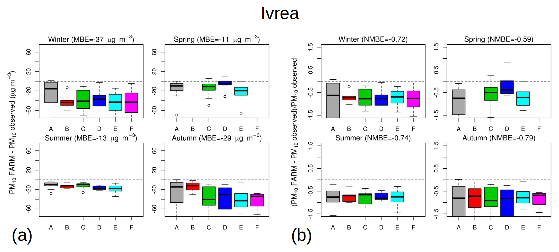
Figure 19Absolute (a) and relative (b) differences between simulated and observed PM10 concentrations at the surface in Ivrea.
Finally, within the limits of the model performances discussed above, we use FARM to extend our observational findings to a wider domain compared to the few measuring sites. In Fig. 20, we provide some summarising plots of 1-year simulations. In particular, these show the 3-D simulated fields of PM10 concentrations in terms of both surface-level (a, b, and c) and vertical transects along the main valley (d, e, and f), averaged over all non-advection and advection days in 2017. In this latter case, simulations with W=1 (b, e) and W=4 (c, f) are included. Compared to the “background condition” (ALC type A), the advection cases show higher PM10 concentrations and a different geographical distribution, increasing towards the entrance of the valley (Fig. 20b, e). Obviously, the absolute PM10 loads are higher when the non-local contribution is multiplied by W=4 (Fig. 20c, f), which, as discussed above, is the W value providing a better matching with the PM10 concentrations actually measured in Aosta and Ivrea. Vertical profiles of simulated concentrations are also evidently impacted by the advections (e.g. Fig. 20d–f). A more complete set of maps is provided in Fig. S12, in which the contribution of particulate produced inside the regional domain (local sources) and outside the domain (boundary conditions) has been partitioned. An interesting feature in Fig. 20 is that the average maps of local PM10 do not change between advection or non-advection cases, while the (relative) concentration maps of aerosol coming from outside the domain show noticeable differences, thus confirming once again that the polluted air masses detected by the ALC in Aosta–Saint-Christophe are of non-local origin. In conclusion, the excellent correspondence between the model output and the experimental classification based on the ALC, i.e. the remarkable difference of the concentrations and their vertical distribution between days of advection and non-advection, highlights both the rather good performances of the CTM and the ability of the measurement dataset used to reveal the phenomenon.
In this work we used long-term (2015–2017) multi-sensor observational datasets (Table 1) coupled to modelling tools to describe pollution aerosol transport from the Po basin to the northwestern Alps. Key to this study was the deployment in Aosta of an automated lidar ceilometer (ALC) with its operational (24/7) capabilities. This allowed us to (a) collect and present the first long-term dataset of aerosol vertical distribution in the northwestern Alps; (b) provide observational evidence of the complex structure and dynamics of the atmosphere in the Alpine valleys; and (c) stimulate the investigation of the phenomenon on a 4-D scale with complementing observational and modelling tools. The analysis over the long term allowed us to expand the investigation of specific case studies provided in the companion paper (Diémoz et al., 2019) and answer some key scientific questions (as listed in the Introduction).
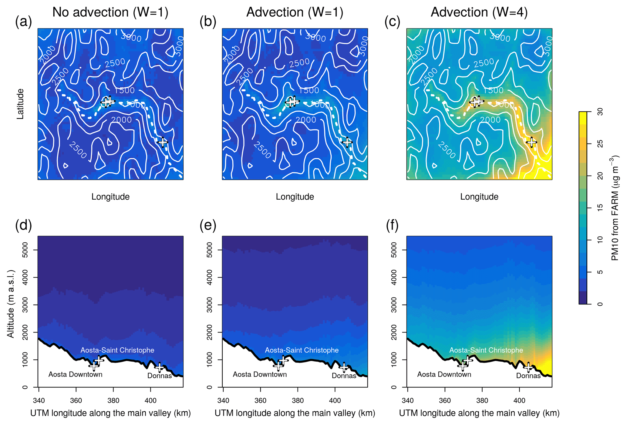
Figure 20Average 3-D fields of PM10 concentration simulated by FARM extracted at the surface level (a, b, c) and on a vertical transect (d, e, f). (a) Average of all non-advection days (categorised as “A” by the experimental ALC classification). (b) Average of advection days (“C”, “E”, and “F” from the ALC classification) using a weighting factor W=1 for the PM10 contribution coming from outside the boundaries of the regional domain. (c) Same as (b) using W=4 as a weighting factor. (d), (e), and (f) are vertical transects along the main valley (i.e. along the dotted line in a to c) corresponding to the three cases above. The altitude of the three measuring sites shown in the panels is the one from the digital elevation model, which is a smoothed representation of the real topography. The white area in the second row of panels represents the surface. The advections investigated in this study come from the east (right side of all the panels).
-
Driving meteorological factors and frequency of the aerosol pollution transport events. The newly developed classification based on the ALC profiles (928 classified days, Fig. 3) permitted us to aggregate the days with similar aerosol vertical structures and examine the average properties of each group. Notably, we could understand the link between the wind flow regimes and the aerosol transport. The frequency of the elevated layers was observed to be on average 43 %–50 % of the days, depending on the season (i.e. slightly less than 60 % of the days falling in an ALC class different from “Other” in winter and spring to more than 70 % in summer) and is clearly connected to eastern wind flows, such as plain-to-mountain, thermally driven winds (blowing nearly 70 % of the days in summer, Fig. 4). This was even clearer using trajectory statistical models (Fig. 13) and contingency tables (Fig. 5) showing the clear connections between the arrival of an elevated aerosol layer over the northwestern Alps and the wind direction. Such layers were observed 93 % of the days with easterly winds (Fig. 5a), with increasing probability of occurrence for increasing air mass residence time over the Po plain (aerosol layer detected on over 80 % of days when the trajectory residence times in the Po basin exceed 1 h, and up to 100 % of days with air mass residence time >10 h, Fig. 5b).
-
Advected aerosol physical and chemical properties. The general spatio-temporal characteristics of the aerosol layers were statistically assessed based on the multi-year ALC series. The top altitudes of the layer range from 500 m to nearly 4000 m a.g.l., depending on season and according to the convective boundary layer height. Notably, the high altitudes reached by the aerosol layer in summer are compatible with transport and deposition of other contaminants, such as pesticides (Rizzi et al., 2019) and micro-plastics (Allen et al., 2019; Ambrosini et al., 2019), on glaciers, snow fields, and remote mountain catchments. Also, a dataset of aerosol layer heights may be valuable for follow-up studies on the radiative forcing of particulate matter in connection with the elevation-dependent warming in some mountain regions (Pepin et al., 2015).
The duration of the phenomenon ranges from a few hours to several days in cases of atmospheric stability. The mean optical and microphysical properties of the aerosol layers were further sounded using a Sun photometer. This showed that the columnar aerosol properties are all impacted by the pollution transport: AOD at 500 nm increases from 0.04 on non-event days up to 0.18 on event days, on average; relevant values of the Ångström exponent (400–870 nm) and single scattering albedo (SSA at 500 nm) change from 1.0 to 1.6 and from 0.92 to 0.98 respectively and depend on the duration/severity of the advection (Fig. 15). This indicates that the transported particles are on average smaller and more light-scattering than the locally produced ones and agrees well with the results of measurements and analyses of aerosol properties at the surface. Positive matrix factorisation (PMF) of chemical properties at surface level revealed that particles advected from the Po Valley to the northwestern Alps are mostly of secondary origin (e.g. Fig. 12) and mainly composed of nitrates, sulfates, and ammonium. Interestingly, we also found an organic component in the warm season, which confirms the Po Valley as an OM source. Moreover, particle size distributions showed increase in the fine fraction (<1 µm) during Po Valley advection days. Correlation of chemical PMF with independent PMF performed on aerosol size distribution also provided evidence of a clear link between chemical properties and aerosol size (correlation indices ρ>0.8, Fig. 14), which proves that different aerosol formation mechanisms act in the atmosphere in different seasons. In particular, we found some evidence of aqueous processing of particles in winter (e.g. fog and/or cloud processing) through identification of a PMF “droplet mode” in the winter results.
-
Aerosol transport impact on air quality. At the bottom of the valley, the advections were demonstrated to alter both the absolute concentrations of PM10 (these being up to 3.5 times higher during event days compared to non-event days, Fig. 8) and their daily cycles, with hourly variations of up to 30 µg m−3 (Fig. 10). PMF statistics on chemical data identified five to seven different sources, depending on the available chemical characterisation, two of which (nitrate-rich mode in winter and sulfate-rich mode in summer) were attributed to the arrival of particles from outside the Aosta Valley, as also confirmed by trajectory statistical models (Fig. 13). Using their relevant scores as a proxy, we estimate an average 25 % contribution of these transported nitrate- and sulfate-rich components to the Aosta PM10. This impact varies on a seasonal basis. The relative contribution of non-local PM10 is highest in summer (32 %), when advection is most frequent and local PM10 is lowest, while it is lowest in winter (16 %), when advection is least frequent and local PM10 is highest. In absolute terms the reverse occurs and the impact of transport is found to be highest in winter/autumn, reaching levels of 50 µg m−3 in some episodes (thus exceeding alone the EU legislative limits). This occurs due to the superposition of advected particles with higher background concentrations in the coldest part of the year, when emissions are highest and pollution is further enhanced by adverse weather conditions, i.e. low-level inversions, locally worsened by the valley topography. In this study the impact of Po Valley advection on air quality was mostly quantified for the Aosta–Downtown station. In rural and remote sites of the region the non-local contribution is expected to be even larger, in relative terms. Increasing the number of stations collecting samples for chemical analyses would be an important follow-up to estimate the non-local contribution to PM10 in non-urban sites. The good correlation found between the PM10 concentration anomalies in the urban site of Aosta–Downtown and in the regional site of Donnas (ρ>0.7, Fig. 9) is however a clear indication that aerosol loads all over the region are mainly influenced by trans-regional transport rather than by local emissions. It is also worth mentioning that the aerosol particle number (here only measured in the 0.18–18 µm range, i.e. missing the finest particles) increased remarkably (up to >3000 particles cm−3) in some transport episodes, with possible implications for human health. Some preliminary results (Sect. S5) also indicate that this regular air mass transport is also able to alter the oxidative capacity of the atmosphere (NOx∕NO ratio), although further investigation is needed to better quantify it.
In general, for both air-quality and climate evaluations the identification of monitoring sites (and time periods) representative of “background conditions” is a critical issue to differentiate local and regional pollution levels (e.g. Yuan et al., 2018). A global network of atmospheric “baseline” monitoring stations is for example maintained within the World Meteorological Organisation's (WMO) Global Atmosphere Watch (GAW) programme (WMO, 2017), with the intention of providing regionally representative measurements relatively free of significant local pollution sources. Our observed (PM10) daily cycle (Figs. 2, 6, and 10) indicates that caution should be paid when assuming mountain sites to be representative of background conditions. In particular, we show that the influence of nearby pollution sources in high-altitude sites might not be limited to the central hours of the day only (when convection-driven growth of the nearby plain mixing layer is known to uplift pollutants), but rather extend to night-time measurements via the mountain–valley circulation and particle growth mechanisms addressed in this study.
-
Ability to predict the arrival and impacts of polluted air mass transport. Experimental data and their coupling with modelling tools well demonstrated the Po plain origin of the polluted layers and their increased probability of detection as a function of the air masses' residence time over the origin region. Current chemical transport models, however, were found to reproduce the phenomenon in qualitative terms, but manifest both systematic underestimations of the absolute advected PM10 (biases) and large scatter to the measurements. Based on two 1-year long simulated datasets in Aosta–Downtown and Ivrea, we tested how the air-quality forecasts could be improved by updating the emission inventories and using the ALC to constrain the modelled emissions. After some sensitivity tests, we tuned the national inventory to better match the measurements (“boundary conditions” increased by a factor of 4). In this case, the model underestimation was reduced from biases to −20 µg m−3 in the worst cases, with mean average biases <2 µg m−3 (Table 3), thus enhancing, on average, our ability to correctly predict the PM concentration and their relevant impacts (Fig. 20). Still, further improvements are necessary to enhance the model's ability to better reproduce aerosol processes (e.g. aqueous-phase chemistry, Gong et al., 2011) and wind fields using higher-resolution NWP models.
In conclusion, we demonstrated that, despite being considered a pristine environment, the northwestern Alps are regularly affected by a sort of “polluted aerosol tide”, i.e. by a wind-driven transport of polluted aerosol layers from the Po plain. Overall, this calls for air pollution mitigation policies acting, at least, over the regional scale in this fragile environment.
The ALC data are available upon request from the Alice-net (alicenet@isac.cnr.it) and E-PROFILE (http://data.ceda.ac.uk/badc/eprofile/data/, E-PROFILE, 2019) networks. The Sun photometer data can be downloaded from the EuroSkyRad network web site (http://www.euroskyrad.net/index.html, EuroSkyRad, 2019) after authentication (credentials may be requested to M. Campanelli, m.campanelli@isac.cnr.it). The measurements from the ARPA Valle d'Aosta air-quality surface network are available on the web page http://www.arpa.vda.it/it/aria/la-qualità-dell-aria/stazioni-di-monitoraggio/inquinanti-export-dati (ARPA Valle d'Aosta, 2019). The PM10 measurements in Ivrea are available on the Piedmont regional government web page http://www.regione.piemonte.it/ambiente/aria/rilev/ariaday/ariaweb-new/index.php/it/home (Regione Piemonte, 2019). The weather data from the Aosta–Saint-Christophe and Saint-Denis stations can be retrieved from http://cf.regione.vda.it/richiesta_dati.php (Centro Funzionale, 2019) upon request to Centro Funzionale della Valle d'Aosta. The rest of the data can be requested from the corresponding author (h.diemoz@arpa.vda.it).
The supplement related to this article is available online at: https://doi.org/10.5194/acp-19-10129-2019-supplement.
HD, FB, and GPG conceived and designed the study, interpreted the results, and wrote the paper. HD analysed the data. TM supplied the meteorological observations and numerical weather predictions. GP performed the chemical transport simulations. SP carried out the EC/OC analyses and IKFT helped with the interpretation of the chemical speciation. MC supplied the POM calibration factors.
The authors declare that they have no conflict of interest.
SKYNET – the international network for aerosol, clouds, and solar radiation studies and their applications (AMT/ACP inter-journal SI) SI statement: this article is part of the special issue “SKYNET – the international network for aerosol, clouds, and solar radiation studies and their applications (AMT/ACP inter-journal SI)”. It is not associated with a conference.
The authors would like to thank Alessandra Brunier, Giuliana Lupato, Paolo Proment, Stefania Vaccari, Maria Cristina Gibellino (ARPA Valle d'Aosta) for carrying out the chemical analyses; Marco Pignet, Claudia Tarricone, and Manuela Zublena (ARPA Valle d'Aosta) for providing the data from the air-quality surface network; and Paolo Lazzeri (APPA Trento) for helping with the PMF analysis. The authors would like to acknowledge the valuable contribution of the discussions in the working group meetings organised by COST Action ES1303 (TOPROF). They also gratefully acknowledge the Institute for Atmospheric and Climate Science, ETH Zurich, Switzerland, for the provision of the LAGRANTO software used in this publication, ARPA Piemonte and Regione Piemonte for the PM10 measurements at the Ivrea station, and two anonymous reviewers whose comments helped improve and clarify the manuscript.
This paper was edited by Pedro Jimenez-Guerrero and reviewed by two anonymous referees.
Agnesod, G., Moulin, P.-A., Pession, G., Villard, H., and Zublena, M.: Étude Air Espace Mont-Blanc – Rapport Technique, Tech. rep., Espace Mont Blanc, available at: http://www.arpa.vda.it/images/stories/ARPA/aria/progetti/progairmb_agnesod_2003.pdf (last access: 2 August 2019), 2003. a
Allen, S., Allen, D., Phoenix, V. R., Le Roux, G., Durántez Jiménez, P., Simonneau, A., Binet, S., and Galop, D.: Atmospheric transport and deposition of microplastics in a remote mountain catchment, Nat. Geosci., 12, 339–344, https://doi.org/10.1038/s41561-019-0335-5, 2019. a, b
Ångström, A.: On the Atmospheric Transmission of Sun Radiation and on Dust in the Air, Geogr. Ann., 11, 156–166, 1929. a
Ambrosini, R., Azzoni, R. S., Pittino, F., Diolaiuti, G., Franzetti, A., and Parolini, M.: First evidence of microplastic contamination in the supraglacial debris of an alpine glacier, Environ. Pollut., 253, 297–301, https://doi.org/10.1016/j.envpol.2019.07.005, 2019. a, b
ARPA Valle d'Aosta: ARPA Valle d'Aosta: Air quality data, available at: http://www.arpa.vda.it/it/aria/la-qualità-dell-aria/stazioni-di-monitoraggio/inquinanti-export-dati, last access: 2 August 2019.
Arvani, B., Bradley Pierce, R., Lyapustin, A. I., Wang, Y., Ghermandi, G., and Teggi, S.: Seasonal monitoring and estimation of regional aerosol distribution over Po valley, northern Italy, using a high-resolution MAIAC product, Atmos. Environ., 141, 106–121, https://doi.org/10.1016/j.atmosenv.2016.06.037, 2016. a, b
Ashbaugh, L. L., Malm, W. C., and Sadeh, W. Z.: A residence time probability analysis of sulfur concentrations at grand Canyon National Park, Atmos. Environ., 19, 1263–1270, https://doi.org/10.1016/0004-6981(85)90256-2, 1985. a
Baldauf, M., Seifert, A., Förstner, J., Majewski, D., Raschendorfer, M., and Reinhardt, T.: Operational Convective-Scale Numerical Weather Prediction with the COSMO Model: Description and Sensitivities, Mon. Weather Rev., 139, 3887–3905, https://doi.org/10.1175/MWR-D-10-05013.1, 2011. a
Barnaba, F. and Gobbi, G. P.: Aerosol seasonal variability over the Mediterranean region and relative impact of maritime, continental and Saharan dust particles over the basin from MODIS data in the year 2001, Atmos. Chem. Phys., 4, 2367–2391, https://doi.org/10.5194/acp-4-2367-2004, 2004. a
Barnaba, F., Gobbi, G. P., and de Leeuw, G.: Aerosol stratification, optical properties and radiative forcing in Venice (Italy) during ADRIEX, Q. J. Roy. Meteor. Soc., 133, 47–60, https://doi.org/10.1002/qj.91, 2007. a
Barnaba, F., Putaud, J. P., Gruening, C., dell'Acqua, A., and Dos Santos, S.: Annual cycle in co-located in situ, total-column, and height-resolved aerosol observations in the Po Valley (Italy): Implications for ground-level particulate matter mass concentration estimation from remote sensing, J. Geophys. Res., 115, D19209, https://doi.org/10.1029/2009JD013002, 2010. a
Barnaba, F., Bolignano, A., Di Liberto, L., Morelli, M., Lucarelli, F., Nava, S., Perrino, C., Canepari, S., Basart, S., Costabile, F., Dionisi, D., Ciampichetti, S., Sozzi, R., and Gobbi, G. P.: Desert dust contribution to PM10 loads in Italy: Methods and recommendations addressing the relevant European Commission Guidelines in support to the Air Quality Directive 2008/50, Atmos. Environ., 161, 288–305, https://doi.org/10.1016/j.atmosenv.2017.04.038, 2017. a
Belis, C., Blond, N., Bouland, C., Carnevale, C., Clappier, A., Douros, J., Fragkou, E., Guariso, G., Miranda, A. I., Nahorski, Z., Pisoni, E., Ponche, J.-L., Thunis, P., Viaene, P., and Volta, M.: Strengths and Weaknesses of the Current EU Situation, Springer International Publishing, 69–83, https://doi.org/10.1007/978-3-319-33349-6_4, 2017. a
Bigi, A. and Ghermandi, G.: Long-term trend and variability of atmospheric PM10 concentration in the Po Valley, Atmos. Chem. Phys., 14, 4895–4907, https://doi.org/10.5194/acp-14-4895-2014, 2014. a, b
Bigi, A. and Ghermandi, G.: Trends and variability of atmospheric PM2.5 and PM10–2.5 concentration in the Po Valley, Italy, Atmos. Chem. Phys., 16, 15777–15788, https://doi.org/10.5194/acp-16-15777-2016, 2016. a
Binkowski, F.: Science Algorithms of the EPA Models-3 Community Multiscale Air Quality (CMAQ) Modeling System, vol. EPA/600/R-99/030, in: The aerosol portion of Models-3 CMAQ, edited by: Byun, D. W. and Ching, J. K. S., 1999. a
Birch, M. E. and Cary, R. A.: Elemental Carbon-Based Method for Monitoring Occupational Exposures to Particulate Diesel Exhaust, Aerosol Sci. Tech., 25, 221–241, https://doi.org/10.1080/02786829608965393, 1996. a
Blyth, S.: Mountain watch: environmental change & sustainable developmental in mountains, United Nations Environment Programme, 2002. a
Bonvalot, L., Tuna, T., Fagault, Y., Jaffrezo, J.-L., Jacob, V., Chevrier, F., and Bard, E.: Estimating contributions from biomass burning, fossil fuel combustion, and biogenic carbon to carbonaceous aerosols in the Valley of Chamonix: a dual approach based on radiocarbon and levoglucosan, Atmos. Chem. Phys., 16, 13753–13772, https://doi.org/10.5194/acp-16-13753-2016, 2016. a
Bourgeois, I., Savarino, J., Caillon, N., Angot, H., Barbero, A., Delbart, F., Voisin, D., and Clément, J.-C.: Tracing the Fate of Atmospheric Nitrate in a Subalpine Watershed Using Δ17O, Environ. Sci. Technol., 52, 5561–5570, https://doi.org/10.1021/acs.est.7b02395, 2018. a
Bressi, M., Sciare, J., Ghersi, V., Mihalopoulos, N., Petit, J.-E., Nicolas, J. B., Moukhtar, S., Rosso, A., Féron, A., Bonnaire, N., Poulakis, E., and Theodosi, C.: Sources and geographical origins of fine aerosols in Paris (France), Atmos. Chem. Phys., 14, 8813–8839, https://doi.org/10.5194/acp-14-8813-2014, 2014. a
Bressi, M., Cavalli, F., Belis, C. A., Putaud, J.-P., Fröhlich, R., Martins dos Santos, S., Petralia, E., Prévôt, A. S. H., Berico, M., Malaguti, A., and Canonaco, F.: Variations in the chemical composition of the submicron aerosol and in the sources of the organic fraction at a regional background site of the Po Valley (Italy), Atmos. Chem. Phys., 16, 12875–12896, https://doi.org/10.5194/acp-16-12875-2016, 2016. a
Brulfert, G., Chemel, C., Chaxel, E., Chollet, J.-P., Jouve, B., and Villard, H.: Assessment of 2010 air quality in two Alpine valleys from modelling: Weather type and emission scenarios, Atmos. Environ., 40, 7893–7907, https://doi.org/10.1016/j.atmosenv.2006.07.021, 2006. a
Bucci, S., Cristofanelli, P., Decesari, S., Marinoni, A., Sandrini, S., Größ, J., Wiedensohler, A., Di Marco, C. F., Nemitz, E., Cairo, F., Di Liberto, L., and Fierli, F.: Vertical distribution of aerosol optical properties in the Po Valley during the 2012 summer campaigns, Atmos. Chem. Phys., 18, 5371–5389, https://doi.org/10.5194/acp-18-5371-2018, 2018. a
Burkhardt, J., Zinsmeister, D., Grantz, D. A., Vidic, S., Sutton, M. A., Hunsche, M., and Pariyar, S.: Camouflaged as degraded wax: hygroscopic aerosols contribute to leaf desiccation, tree mortality, and forest decline, Environ. Res. Lett., 13, 085001, https://doi.org/10.1088/1748-9326/aad346, 2018. a
Centro Funzionale: Centro Funzionale: weather data, available at: http://cf.regione.vda.it/richiesta_dati.php, last access: 2 August 2019.
Calori, G., Silibello, C., and Marras, G.: FARM (Flexible Air quality Regional Model) Model formulation and user's Manual, Arianet, 4.7 edn., 2014. a
Campana, M., Li, Y., Staehelin, J., Prevot, A. S., Bonasoni, P., Loetscher, H., and Peter, T.: The influence of south foehn on the ozone mixing ratios at the high alpine site Arosa, Atmos. Environ., 39, 2945–2955, https://doi.org/10.1016/j.atmosenv.2005.01.037, 2005. a
Campanelli, M., Estellés, V., Tomasi, C., Nakajima, T., Malvestuto, V., and Martínez-Lozano, J. A.: Application of the SKYRAD Improved Langley plot method for the in situ calibration of CIMEL Sun-sky photometers, Appl. Opt., 46, 2688–2702, https://doi.org/10.1364/AO.46.002688, 2007. a
Campanelli, M., Mascitelli, A., Sanò, P., Diémoz, H., Estellés, V., Federico, S., Iannarelli, A. M., Fratarcangeli, F., Mazzoni, A., Realini, E., Crespi, M., Bock, O., Martínez-Lozano, J. A., and Dietrich, S.: Precipitable water vapour content from ESR/SKYNET sun-sky radiometers: validation against GNSS/GPS and AERONET over three different sites in Europe, Atmos. Meas. Tech., 11, 81–94, https://doi.org/10.5194/amt-11-81-2018, 2018. a
Carbone, C., Decesari, S., Mircea, M., Giulianelli, L., Finessi, E., Rinaldi, M., Fuzzi, S., Marinoni, A., Duchi, R., Perrino, C., Sargolini, T., Vardè, M., Sprovieri, F., Gobbi, G., Angelini, F., and Facchini, M.: Size-resolved aerosol chemical composition over the Italian Peninsula during typical summer and winter conditions, Atmos. Environ., 44, 5269–5278, https://doi.org/10.1016/j.atmosenv.2010.08.008, 2010. a
Carslaw, K. S., Boucher, O., Spracklen, D. V., Mann, G. W., Rae, J. G. L., Woodward, S., and Kulmala, M.: A review of natural aerosol interactions and feedbacks within the Earth system, Atmos. Chem. Phys., 10, 1701–1737, https://doi.org/10.5194/acp-10-1701-2010, 2010. a
Cavalli, F., Viana, M., Yttri, K. E., Genberg, J., and Putaud, J.-P.: Toward a standardised thermal-optical protocol for measuring atmospheric organic and elemental carbon: the EUSAAR protocol, Atmos. Meas. Tech., 3, 79–89, https://doi.org/10.5194/amt-3-79-2010, 2010. a
Cesaroni, G., Badaloni, C., Gariazzo, C., Stafoggia, M., Sozzi, R., Davoli, M., and Forastiere, F.: Long-term exposure to urban air pollution and mortality in a cohort of more than a million adults in Rome, Environ. Health Persp., 121, 324–331, https://doi.org/10.1289/ehp.1205862, 2013. a
Charron, A., Harrison, R. M., Moorcroft, S., and Booker, J.: Quantitative interpretation of divergence between PM10 and PM2.5 mass measurement by TEOM and gravimetric (Partisol) instruments, Atmos. Environ., 38, 415–423, https://doi.org/10.1016/j.atmosenv.2003.09.072, 2004. a
Chazette, P., Couvert, P., Randriamiarisoa, H., Sanak, J., Bonsang, B., Moral, P., Berthier, S., Salanave, S., and Toussaint, F.: Three-dimensional survey of pollution during winter in French Alps valleys, Atmos. Environ., 39, 1035–1047, https://doi.org/10.1016/j.atmosenv.2004.10.014, 2005. a
Chemel, C., Arduini, G., Staquet, C., Largeron, Y., Legain, D., Tzanos, D., and Paci, A.: Valley heat deficit as a bulk measure of wintertime particulate air pollution in the Arve River Valley, Atmos. Environ., 128, 208–215, https://doi.org/10.1016/j.atmosenv.2015.12.058, 2016. a
Chu, D. A., Kaufman, Y. J., Zibordi, G., Chern, J. D., Mao, J., Li, C., and Holben, B. N.: Global monitoring of air pollution over land from the Earth Observing System-Terra Moderate Resolution Imaging Spectroradiometer (MODIS), J. Geophys. Res., 108, 4661, https://doi.org/10.1029/2002JD003179, 2003. a
Clerici, M. and Mélin, F.: Aerosol direct radiative effect in the Po Valley region derived from AERONET measurements, Atmos. Chem. Phys., 8, 4925–4946, https://doi.org/10.5194/acp-8-4925-2008, 2008. a, b
Cong, Z., Kawamura, K., Kang, S., and Fu, P.: Penetration of biomass-burning emissions from South Asia through the Himalayas: new insights from atmospheric organic acids, Sci. Rep., 5, 9580, https://doi.org/10.1038/srep09580, 2015. a
Costabile, F., Gilardoni, S., Barnaba, F., Di Ianni, A., Di Liberto, L., Dionisi, D., Manigrasso, M., Paglione, M., Poluzzi, V., Rinaldi, M., Facchini, M. C., and Gobbi, G. P.: Characteristics of brown carbon in the urban Po Valley atmosphere, Atmos. Chem. Phys., 17, 313–326, https://doi.org/10.5194/acp-17-313-2017, 2017. a, b, c
Cugerone, K., De Michele, C., Ghezzi, A., Gianelle, V., and Gilardoni, S.: On the functional form of particle number size distributions: influence of particle source and meteorological variables, Atmos. Chem. Phys., 18, 4831–4842, https://doi.org/10.5194/acp-18-4831-2018, 2018. a
Curci, G., Ferrero, L., Tuccella, P., Barnaba, F., Angelini, F., Bolzacchini, E., Carbone, C., Denier van der Gon, H. A. C., Facchini, M. C., Gobbi, G. P., Kuenen, J. P. P., Landi, T. C., Perrino, C., Perrone, M. G., Sangiorgi, G., and Stocchi, P.: How much is particulate matter near the ground influenced by upper-level processes within and above the PBL? A summertime case study in Milan (Italy) evidences the distinctive role of nitrate, Atmos. Chem. Phys., 15, 2629–2649, https://doi.org/10.5194/acp-15-2629-2015, 2015. a
Decesari, S., Allan, J., Plass-Duelmer, C., Williams, B. J., Paglione, M., Facchini, M. C., O'Dowd, C., Harrison, R. M., Gietl, J. K., Coe, H., Giulianelli, L., Gobbi, G. P., Lanconelli, C., Carbone, C., Worsnop, D., Lambe, A. T., Ahern, A. T., Moretti, F., Tagliavini, E., Elste, T., Gilge, S., Zhang, Y., and Dall'Osto, M.: Measurements of the aerosol chemical composition and mixing state in the Po Valley using multiple spectroscopic techniques, Atmos. Chem. Phys., 14, 12109–12132, https://doi.org/10.5194/acp-14-12109-2014, 2014. a, b
de Freitas, C. R.: Tourism climatology: evaluating environmental information for decision making and business planning in the recreation and tourism sector, Int. J. Biometeorol., 48, 45–54, https://doi.org/10.1007/s00484-003-0177-z, 2003. a
De Wekker, S. F. J. and Kossmann, M.: Convective Boundary Layer Heights Over Mountainous Terrain–A Review of Concepts, Front. Earth Sci., 3, 77, https://doi.org/10.3389/feart.2015.00077, 2015. a
Dhungel, S., Kathayat, B., Mahata, K., and Panday, A.: Transport of regional pollutants through a remote trans-Himalayan valley in Nepal, Atmos. Chem. Phys., 18, 1203–1216, https://doi.org/10.5194/acp-18-1203-2018, 2018. a
Diémoz, H., Siani, A. M., Casale, G. R., di Sarra, A., Serpillo, B., Petkov, B., Scaglione, S., Bonino, A., Facta, S., Fedele, F., Grifoni, D., Verdi, L., and Zipoli, G.: First national intercomparison of solar ultraviolet radiometers in Italy, Atmos. Meas. Tech., 4, 1689–1703, https://doi.org/10.5194/amt-4-1689-2011, 2011. a
Diémoz, H., Campanelli, M., and Estellés, V.: One Year of Measurements with a POM-02 Sky Radiometer at an Alpine EuroSkyRad Station, J. Meteorol. Soc. Jpn., 92A, 1–16, https://doi.org/10.2151/jmsj.2014-A01, 2014a. a
Diémoz, H., Siani, A. M., Redondas, A., Savastiouk, V., McElroy, C. T., Navarro-Comas, M., and Hase, F.: Improved retrieval of nitrogen dioxide (NO2) column densities by means of MKIV Brewer spectrophotometers, Atmos. Meas. Tech., 7, 4009–4022, https://doi.org/10.5194/amt-7-4009-2014, 2014b. a
Diémoz, H., Barnaba, F., Magri, T., Pession, G., Dionisi, D., Pittavino, S., Tombolato, I. K. F., Campanelli, M., Della Ceca, L. S., Hervo, M., Di Liberto, L., Ferrero, L., and Gobbi, G. P.: Transport of Po Valley aerosol pollution to the northwestern Alps – Part 1: Phenomenology, Atmos. Chem. Phys., 19, 3065–3095, https://doi.org/10.5194/acp-19-3065-2019, 2019. a, b, c, d, e, f, g, h, i, j, k
Dionisi, D., Barnaba, F., Diémoz, H., Di Liberto, L., and Gobbi, G. P.: A multiwavelength numerical model in support of quantitative retrievals of aerosol properties from automated lidar ceilometers and test applications for AOT and PM10 estimation, Atmos. Meas. Tech., 11, 6013–6042, https://doi.org/10.5194/amt-11-6013-2018, 2018. a
Dosio, A., Galmarini, S., and Graziani, G.: Simulation of the circulation and related photochemical ozone dispersion in the Po plains (northern Italy): Comparison with the observations of a measuring campaign, J. Geophys. Res., 107, LOP 2-1–LOP 2-24, https://doi.org/10.1029/2000JD000046, 2002. a
EEA: Air Quality in Europe – 2015 Report, Tech. rep., https://doi.org/10.2800/62459, 2015. a
EEA: Air Quality in Europe – 2017 Report, Tech. rep., https://doi.org/10.2800/850018, 2017. a
E-PROFILE: ALC data, available at: http://data.ceda.ac.uk/badc/eprofile/data/, last access: 2 August 2019.
EuroSkyRad: Sun-sky radiometer data, available at: http://www.euroskyrad.net/index.html, last access: 2 August 2019.
Egger, J., Bajrachaya, S., Egger, U., Heinrich, R., Reuder, J., Shayka, P., Wendt, H., and Wirth, V.: Diurnal Winds in the Himalayan Kali Gandaki Valley. Part I: Observations, Mon. Weather Rev., 128, 1106–1122, https://doi.org/10.1175/1520-0493(2000)128<1106:DWITHK>2.0.CO;2, 2000. a
EMEP: Transboundary particulate matter, photo-oxidants, acidifying and eutrophying components, Tech. rep., MSC-W, CCC and CEIP, 2016. a, b
EU Commission: Directive 2008/50/EC of the European Parliament and of the Council of 21 May 2008 on ambient air quality and cleaner air for Europe, Official Journal of the European Union, L152/1–44, 2008. a
EU Commission: European Commission – Press release: Air quality: Commission takes action to protect citizens from air pollution, Brussels, 17 May 2018, Press Release Database, available at: http://europa.eu/rapid/press-release_IP-18-3450_en.htm (last access: 2 August 2019), 2018. a
Fernald, F. G.: Analysis of atmospheric lidar observations: some comments, Appl. Opt., 23, 652–653, https://doi.org/10.1364/AO.23.000652, 1984. a
Ferrero, L., Perrone, M. G., Petraccone, S., Sangiorgi, G., Ferrini, B. S., Lo Porto, C., Lazzati, Z., Cocchi, D., Bruno, F., Greco, F., Riccio, A., and Bolzacchini, E.: Vertically-resolved particle size distribution within and above the mixing layer over the Milan metropolitan area, Atmos. Chem. Phys., 10, 3915–3932, https://doi.org/10.5194/acp-10-3915-2010, 2010. a
Ferrero, L., Castelli, M., Ferrini, B. S., Moscatelli, M., Perrone, M. G., Sangiorgi, G., D'Angelo, L., Rovelli, G., Moroni, B., Scardazza, F., Močnik, G., Bolzacchini, E., Petitta, M., and Cappelletti, D.: Impact of black carbon aerosol over Italian basin valleys: high-resolution measurements along vertical profiles, radiative forcing and heating rate, Atmos. Chem. Phys., 14, 9641–9664, https://doi.org/10.5194/acp-14-9641-2014, 2014. a
Finardi, S., Silibello, C., D'Allura, A., and Radice, P.: Analysis of pollutants exchange between the Po Valley and the surrounding European region, Urban Clim., 10, 682–702, https://doi.org/10.1016/j.uclim.2014.02.002, 2014. a
Fuzzi, S., Baltensperger, U., Carslaw, K., Decesari, S., Denier van der Gon, H., Facchini, M. C., Fowler, D., Koren, I., Langford, B., Lohmann, U., Nemitz, E., Pandis, S., Riipinen, I., Rudich, Y., Schaap, M., Slowik, J. G., Spracklen, D. V., Vignati, E., Wild, M., Williams, M., and Gilardoni, S.: Particulate matter, air quality and climate: lessons learned and future needs, Atmos. Chem. Phys., 15, 8217–8299, https://doi.org/10.5194/acp-15-8217-2015, 2015. a
Gariazzo, C., Silibello, C., Finardi, S., Radice, P., Piersanti, A., Calori, G., Cecinato, A., Perrino, C., Nussio, F., Cagnoli, M., Pelliccioni, A., Gobbi, G. P., and Di Filippo, P.: A gas/aerosol air pollutants study over the urban area of Rome using a comprehensive chemical transport model, Atmos. Environ., 41, 7286–7303, https://doi.org/10.1016/j.atmosenv.2007.05.018, 2007. a
Gilardoni, S., Vignati, E., Cavalli, F., Putaud, J. P., Larsen, B. R., Karl, M., Stenström, K., Genberg, J., Henne, S., and Dentener, F.: Better constraints on sources of carbonaceous aerosols using a combined 14C – macro tracer analysis in a European rural background site, Atmos. Chem. Phys., 11, 5685–5700, https://doi.org/10.5194/acp-11-5685-2011, 2011. a
Gilardoni, S., Massoli, P., Giulianelli, L., Rinaldi, M., Paglione, M., Pollini, F., Lanconelli, C., Poluzzi, V., Carbone, S., Hillamo, R., Russell, L. M., Facchini, M. C., and Fuzzi, S.: Fog scavenging of organic and inorganic aerosol in the Po Valley, Atmos. Chem. Phys., 14, 6967–6981, https://doi.org/10.5194/acp-14-6967-2014, 2014. a
Gilardoni, S., Massoli, P., Paglione, M., Giulianelli, L., Carbone, C., Rinaldi, M., Decesari, S., Sandrini, S., Costabile, F., Gobbi, G. P., Pietrogrande, M. C., Visentin, M., Scotto, F., Fuzzi, S., and Facchini, M. C.: Direct observation of aqueous secondary organic aerosol from biomass-burning emissions, P. Natl. A. Sci. USA, 113, 10013–10018, https://doi.org/10.1073/pnas.1602212113, 2016. a
Giovannini, L., Antonacci, G., Zardi, D., Laiti, L., and Panziera, L.: Sensitivity of Simulated Wind Speed to Spatial Resolution over Complex Terrain, Energy Proced., 59, 323–329, https://doi.org/10.1016/j.egypro.2014.10.384, 2014. a
Giovannini, L., Laiti, L., Serafin, S., and Zardi, D.: The thermally driven diurnal wind system of the Adige Valley in the Italian Alps, Q. J. Roy. Meteor. Soc., 143, 2389–2402, https://doi.org/10.1002/qj.3092, 2017. a
Gohm, A., Harnisch, F., Vergeiner, J., Obleitner, F., Schnitzhofer, R., Hansel, A., Fix, A., Neininger, B., Emeis, S., and Schäfer, K.: Air Pollution Transport in an Alpine Valley: Results From Airborne and Ground-Based Observations, Bound.-Lay. Meteorol., 131, 441–463, https://doi.org/10.1007/s10546-009-9371-9, 2009. a
Golzio, A. and Pelfini, M.: High resolution WRF over mountainous complex terrain: testing over the Ortles Cevedale area (Central Italian Alps), in: Conference: First National Congress, Italian Association of Atmospheric Sciences and Meteorology (AISAM), AISAM, 2018. a
Golzio, A., Ferrarese, S., Cassardo, C., Diolaiuti, G. A., and Pelfini, M.: Grid-size comparison of WRF model over complex mountainous terrain with topography and land-use improvements, Bound.-Lay. Meteorol., submission ID BOUND-D-19-00125, 2019. a
Gong, W., Stroud, C., and Zhang, L.: Cloud Processing of Gases and Aerosols in Air Quality Modeling, Atmosphere, 2, 567–616, https://doi.org/10.3390/atmos2040567, 2011. a
Green, D. C., Fuller, G. W., and Baker, T.: Development and validation of the volatile correction model for PM10 – An empirical method for adjusting TEOM measurements for their loss of volatile particulate matter, Atmos. Environ., 43, 2132–2141, https://doi.org/10.1016/j.atmosenv.2009.01.024, 2009. a
Hann, J. V.: Zur Theorie der Berg- und Talwinde, Z. Öst. Meteorol., 14, 444–448, 1879. a
Harrison, R. M., Jones, A. M., Gietl, J., Yin, J., and Green, D. C.: Estimation of the Contributions of Brake Dust, Tire Wear, and Resuspension to Nonexhaust Traffic Particles Derived from Atmospheric Measurements, Environ. Sci. Technol., 46, 6523–6529, https://doi.org/10.1021/es300894r, 2012. a
Hashimoto, M., Nakajima, T., Dubovik, O., Campanelli, M., Che, H., Khatri, P., Takamura, T., and Pandithurai, G.: Development of a new data-processing method for SKYNET sky radiometer observations, Atmos. Meas. Tech., 5, 2723–2737, https://doi.org/10.5194/amt-5-2723-2012, 2012. a
Hsu, Y.-K., Holsen, T. M., and Hopke, P. K.: Comparison of hybrid receptor models to locate PCB sources in Chicago, Atmos. Environ., 37, 545–562, https://doi.org/10.1016/S1352-2310(02)00886-5, 2003. a
Kabashnikov, V. P., Chaikovsky, A., P., Kucsera, T. L., and Metelskaya, N. S.: Estimated accuracy of three common trajectory statistical methods, Atmos. Environ., 45, 5425–5430, https://doi.org/10.1016/j.atmosenv.2011.07.006, 2011. a
Kaiser, A.: Origin of polluted air masses in the Alps. An overview and first results for MONARPOP, Environ. Pollut., 157, 3232–3237, https://doi.org/10.1016/j.envpol.2009.05.042, 2009. a
Kambezidis, H. and Kaskaoutis, D.: Aerosol climatology over four AERONET sites: An overview, Atmos. Environ., 42, 1892–1906, https://doi.org/10.1016/j.atmosenv.2007.11.013, 2008. a
Kastendeuch, P. P. and Kaufmann, P.: Classification of summer wind fields over complex terrain, Int. J. Climatol., 17, 521–534, https://doi.org/10.1002/(SICI)1097-0088(199704)17:5<521::AID-JOC143>3.0.CO;2-Q, 1997. a
Kazadzis, S., Kouremeti, N., Diémoz, H., Gröbner, J., Forgan, B. W., Campanelli, M., Estellés, V., Lantz, K., Michalsky, J., Carlund, T., Cuevas, E., Toledano, C., Becker, R., Nyeki, S., Kosmopoulos, P. G., Tatsiankou, V., Vuilleumier, L., Denn, F. M., Ohkawara, N., Ijima, O., Goloub, P., Raptis, P. I., Milner, M., Behrens, K., Barreto, A., Martucci, G., Hall, E., Wendell, J., Fabbri, B. E., and Wehrli, C.: Results from the Fourth WMO Filter Radiometer Comparison for aerosol optical depth measurements, Atmos. Chem. Phys., 18, 3185–3201, https://doi.org/10.5194/acp-18-3185-2018, 2018. a
Keiser, D., Lade, G., and Rudik, I.: Air pollution and visitation at U.S. national parks, Sci. Adv., 4, 7, https://doi.org/10.1126/sciadv.aat1613, 2018. a
Khan, M., Masiol, M., Formenton, G., Di Gilio, A., de Gennaro, G., Agostinelli, C., and Pavoni, B.: Carbonaceous PM2.5 and secondary organic aerosol across the Veneto region (NE Italy), Sci. Total Environ., 542, 172–181, https://doi.org/10.1016/j.scitotenv.2015.10.103, 2016. a
Khatri, P. and Takamura, T.: An Algorithm to Screen Cloud-Affected Data for Sky Radiometer Data Analysis, J. Meteorol. Soc. Jpn., 87, 189–204, https://doi.org/10.2151/jmsj.87.189, 2009. a
Klett, J. D.: Lidar inversion with variable backscatter/extinction ratios, Appl. Opt., 24, 1638–1643, https://doi.org/10.1364/AO.24.001638, 1985. a
Kukkonen, J., Sokhi, R., Luhana, L., Härkönen, J., Salmi, T., Sofiev, M., and Karppinen, A.: Evaluation and application of a statistical model for assessment of long-range transported proportion of PM2.5 in the United Kingdom and in Finland, Atmos. Environ., 42, 3980–3991, https://doi.org/10.1016/j.atmosenv.2007.02.036, 2008. a
Landi, T., Curci, G., Carbone, C., Menut, L., Bessagnet, B., Giulianelli, L., Paglione, M., and Facchini, M.: Simulation of size-segregated aerosol chemical composition over northern Italy in clear sky and wind calm conditions, Atmos. Res., 125–126, 1–11, https://doi.org/10.1016/j.atmosres.2013.01.009, 2013. a
Largeron, Y. and Staquet, C.: Persistent inversion dynamics and wintertime PM10 air pollution in Alpine valleys, Atmos. Environ., 135, 92–108, https://doi.org/10.1016/j.atmosenv.2016.03.045, 2016. a
Larsen, B., Gilardoni, S., Stenström, K., Niedzialek, J., Jimenez, J., and Belis, C.: Sources for PM air pollution in the Po Plain, Italy: II. Probabilistic uncertainty characterization and sensitivity analysis of secondary and primary sources, Atmos. Environ., 50, 203–213, https://doi.org/10.1016/j.atmosenv.2011.12.038, 2012. a
Loomis, D., Grosse, Y., Lauby-Secretan, B., El Ghissassi, F., Bouvard, V., Benbrahim-Tallaa, L., Guha, N., Baan, R., Mattock, H., and Straif, K.: The carcinogenicity of outdoor air pollution, Lancet Oncol., 14, 1262, https://doi.org/10.1016/S1470-2045(13)70487-X, 2013. a
Mann, H. B. and Whitney, D. R.: On a Test of Whether one of Two Random Variables is Stochastically Larger than the Other, Ann. Math. Stat., 18, 50–60, 1947. a
Matta, E., Facchini, M. C., Decesari, S., Mircea, M., Cavalli, F., Fuzzi, S., Putaud, J.-P., and Dell'Acqua, A.: Mass closure on the chemical species in size-segregated atmospheric aerosol collected in an urban area of the Po Valley, Italy, Atmos. Chem. Phys., 3, 623–637, https://doi.org/10.5194/acp-3-623-2003, 2003. a
Mazzola, M., Lanconelli, C., Lupi, A., Busetto, M., Vitale, V., and Tomasi, C.: Columnar aerosol optical properties in the Po Valley, Italy, from MFRSR data, J. Geophys. Res., 115, D17206, https://doi.org/10.1029/2009JD013310, 2010. a
Mélin, F. and Zibordi, G.: Aerosol variability in the Po Valley analyzed from automated optical measurements, Geophy. Res. Lett., 32, L03810, https://doi.org/10.1029/2004GL021787, 2005. a
Norris, G. and Duvall, R.: EPA Positive Matrix Factorization (PMF) 5.0 – Fundamentals and User Guide, U.S. Environmental Protection Agency, available at: https://www.epa.gov/sites/production/files/2015-02/documents/pmf_5.0_user_guide.pdf (last access: 2 August 2019), 2014. a, b
Nyeki, S., Eleftheriadis, K., Baltensperger, U., Colbeck, I., Fiebig, M., Fix, A., Kiemle, C., Lazaridis, M., and Petzold, A.: Airborne Lidar and in-situ Aerosol Observations of an Elevated Layer, Leeward of the European Alps and Apennines, Geophys. Res. Lett., 29, 33-1–33-4, https://doi.org/10.1029/2002GL014897, 2002. a
Paatero, P.: Least squares formulation of robust non-negative factor analysis, Chemometr. Intell. Lab., 37, 23–35, https://doi.org/10.1016/S0169-7439(96)00044-5, 1997. a
Paatero, P. and Tapper, U.: Positive matrix factorization: A non-negative factor model with optimal utilization of error estimates of data values, Environmetrics, 5, 111–126, https://doi.org/10.1002/env.3170050203, 1994. a
Patashnick, H. and Rupprecht, E. G.: Continuous PM-10 Measurements Using the Tapered Element Oscillating Microbalance, J. Air Waste Manage., 41, 1079–1083, https://doi.org/10.1080/10473289.1991.10466903, 1991. a
Pepin, N., Bradley, R. S., Diaz, H. F., Baraer, M., Caceres, E. B., Forsythe, N., Fowler, H., Greenwood, G., Hashmi, M. Z., Liu, X. D., Miller, J. R., Ning, L., Ohmura, A., Palazzi, E., Rangwala, I., Schöner, W., Severskiy, I., Shahgedanova, M., Wang, M. B., Williamson, S. N., and Yang, D. Q.: Elevation-dependent warming in mountain regions of the world, Nat. Clim. Change, 5, 424–430, https://doi.org/10.1038/nclimate2563, 2015. a, b
Perrone, M., Larsen, B., Ferrero, L., Sangiorgi, G., De Gennaro, G., Udisti, R., Zangrando, R., Gambaro, A., and Bolzacchini, E.: Sources of high PM2.5 concentrations in Milan, Northern Italy: Molecular marker data and CMB modelling, Sci. Total Environ., 414, 343–355, https://doi.org/10.1016/j.scitotenv.2011.11.026, 2012. a
Philipona, R.: Greenhouse warming and solar brightening in and around the Alps, Int. J. Climatol., 33, 1530–1537, https://doi.org/10.1002/joc.3531, 2013. a
Pletscher, K., Weiss, M., and Moelter, L.: Simultaneous determination of PM fractions, particle number and particle size distribution in high time resolution applying one and the same optical measurement technique, Gefahrst. Reinhalt. L., 76, 425–436, available at: http://www.gefahrstoffe.de/gest/article.php?data[article_id]=86622 (last access: 2 August 2019), 2016. a
Putaud, J. P., Van Dingenen, R., and Raes, F.: Submicron aerosol mass balance at urban and semirural sites in the Milan area (Italy), J. Geophys. Res., 107, LOP 11-1–LOP 11-10, https://doi.org/10.1029/2000JD000111, 2002. a, b
Putaud, J.-P., Dingenen, R. V., Alastuey, A., Bauer, H., Birmili, W., Cyrys, J., Flentje, H., Fuzzi, S., Gehrig, R., Hansson, H., Harrison, R., Herrmann, H., Hitzenberger, R., Hüglin, C., Jones, A., Kasper-Giebl, A., Kiss, G., Kousa, A., Kuhlbusch, T., Löschau, G., Maenhaut, W., Molnar, A., Moreno, T., Pekkanen, J., Perrino, C., Pitz, M., Puxbaum, H., Querol, X., Rodriguez, S., Salma, I., Schwarz, J., Smolik, J., Schneider, J., Spindler, G., ten Brink, H., Tursic, J., Viana, M., Wiedensohler, A., and Raes, F.: A European aerosol phenomenology – 3: Physical and chemical characteristics of particulate matter from 60 rural, urban, and kerbside sites across Europe, Atmos. Environ., 44, 1308–1320, https://doi.org/10.1016/j.atmosenv.2009.12.011, 2010. a
Putaud, J. P., Cavalli, F., Martins dos Santos, S., and Dell'Acqua, A.: Long-term trends in aerosol optical characteristics in the Po Valley, Italy, Atmos. Chem. Phys., 14, 9129–9136, https://doi.org/10.5194/acp-14-9129-2014, 2014. a
Ramanathan, V., Crutzen, P. J., Kiehl, J. T., and Rosenfeld, D.: Aerosols, Climate, and the Hydrological Cycle, Science, 294, 2119–2124, https://doi.org/10.1126/science.1064034, 2001. a
Regione Piemonte: Air quality data, available at: http://www.regione.piemonte.it/ambiente/aria/rilev/ariaday/ariaweb-new/index.php/it/home, last access: 2 August 2019.
Rizzi, C., Finizio, A., Maggi, V., and Villa, S.: Spatial-temporal analysis and risk characterisation of pesticides in Alpine glacial streams, Environ. Pollut., 248, 659–666, https://doi.org/10.1016/j.envpol.2019.02.067, 2019. a, b
Rosati, B., Gysel, M., Rubach, F., Mentel, T. F., Goger, B., Poulain, L., Schlag, P., Miettinen, P., Pajunoja, A., Virtanen, A., Klein Baltink, H., Henzing, J. S. B., Größ, J., Gobbi, G. P., Wiedensohler, A., Kiendler-Scharr, A., Decesari, S., Facchini, M. C., Weingartner, E., and Baltensperger, U.: Vertical profiling of aerosol hygroscopic properties in the planetary boundary layer during the PEGASOS campaigns, Atmos. Chem. Phys., 16, 7295–7315, https://doi.org/10.5194/acp-16-7295-2016, 2016. a
Saarikoski, S., Carbone, S., Decesari, S., Giulianelli, L., Angelini, F., Canagaratna, M., Ng, N. L., Trimborn, A., Facchini, M. C., Fuzzi, S., Hillamo, R., and Worsnop, D.: Chemical characterization of springtime submicrometer aerosol in Po Valley, Italy, Atmos. Chem. Phys., 12, 8401–8421, https://doi.org/10.5194/acp-12-8401-2012, 2012. a, b, c
Sabatier, T., Paci, A., Canut, G., Largeron, Y., Dabas, A., Donier, J.-M., and Douffet, T.: Wintertime Local Wind Dynamics from Scanning Doppler Lidar and Air Quality in the Arve River Valley, Atmosphere, 9, 118, https://doi.org/10.3390/atmos9040118, 2018. a
Samset, B. H.: How cleaner air changes the climate, Science, 360, 148–150, https://doi.org/10.1126/science.aat1723, 2018. a
Sandrini, S., Fuzzi, S., Piazzalunga, A., Prati, P., Bonasoni, P., Cavalli, F., Bove, M. C., Calvello, M., Cappelletti, D., Colombi, C., Contini, D., de Gennaro, G., Di Gilio, A., Fermo, P., Ferrero, L., Gianelle, V., Giugliano, M., Ielpo, P., Lonati, G., Marinoni, A., Massabò, D., Molteni, U., Moroni, B., Pavese, G., Perrino, C., Perrone, M. G., Perrone, M. R., Putaud, J.-P., Sargolini, T., Vecchi, R., and Gilardoni, S.: Spatial and seasonal variability of carbonaceous aerosol across Italy, Atmos. Environ., 99, 587–598, https://doi.org/10.1016/j.atmosenv.2014.10.032, 2014. a
Schaap, M., van Loon, M., ten Brink, H. M., Dentener, F. J., and Builtjes, P. J. H.: Secondary inorganic aerosol simulations for Europe with special attention to nitrate, Atmos. Chem. Phys., 4, 857–874, https://doi.org/10.5194/acp-4-857-2004, 2004. a
Schmidli, J.: Daytime Heat Transfer Processes over Mountainous Terrain, J. Atmos. Sci., 70, 4041–4066, https://doi.org/10.1175/JAS-D-13-083.1, 2013. a
Schmidli, J., Böing, S., and Fuhrer, O.: Accuracy of Simulated Diurnal Valley Winds in the Swiss Alps: Influence of Grid Resolution, Topography Filtering, and Land Surface Datasets, Atmosphere, 9, 196, https://doi.org/10.3390/atmos9050196, 2018. a, b
Seibert, P.: The riddles of foehn – introduction to the historic articles by Hann and Ficker, Meteorol. Z., 21, 607–614, https://doi.org/10.1127/0941-2948/2012/0398, 2012. a
Seibert, P., Kromp-Kolb, H., Baltensperger, U., Jost, D. T., and Schwikowski, M.: Trajectory Analysis of High-Alpine Air Pollution Data, Springer US, Boston, MA, 595–596, https://doi.org/10.1007/978-1-4615-1817-4_65, 1994. a
Seibert, P., Kromp-kolb, H., Kasper, A., Kalina, M., Puxbaum, H., Jost, D. T., Schwikowski, M., and Baltensperger, U.: Transport of polluted boundary layer air from the Po Valley to high-alpine sites, Atmos. Environ., 32, 3953–3965, https://doi.org/10.1016/S1352-2310(97)00174-X, 1998. a
Seinfeld, J. H. and Pandis, S. N.: Atmospheric Chemistry and Physics: From Air Pollution to Climate Change – 2nd ed., John Wiley & Sons, 2006. a
Serafin, S. and Zardi, D.: Daytime Heat Transfer Processes Related to Slope Flows and Turbulent Convection in an Idealized Mountain Valley, J. Atmos. Sci., 67, 3739–3756, https://doi.org/10.1175/2010JAS3428.1, 2010. a
Serafin, S., Adler, B., Cuxart, J., De Wekker, S. F. J., Gohm, A., Grisogono, B., Kalthoff, N., Kirshbaum, D. J., Rotach, M. W., Schmidli, J., Stiperski, I., Večenaj, Ž., and Zardi, D.: Exchange Processes in the Atmospheric Boundary Layer Over Mountainous Terrain, Atmosphere, 9, 102, https://doi.org/10.3390/atmos9030102, 2018. a
Silibello, C., Calori, G., Brusasca, G., Giudici, A., Angelino, E., Fossati, G., Peroni, E., and Buganza, E.: Modelling of PM10 concentrations over Milano urban area using two aerosol modules, Environ. Modell. Softw., 23, 333–343, https://doi.org/10.1016/j.envsoft.2007.04.002, 2008. a
Skamarock, W. C.: Evaluating Mesoscale NWP Models Using Kinetic Energy Spectra, Mon. Weather Rev., 132, 3019–3032, https://doi.org/10.1175/MWR2830.1, 2004. a
Sprenger, M. and Wernli, H.: The LAGRANTO Lagrangian analysis tool – version 2.0, Geosci. Model Dev., 8, 2569–2586, https://doi.org/10.5194/gmd-8-2569-2015, 2015 a
Squizzato, S. and Masiol, M.: Application of meteorology-based methods to determine local and external contributions to particulate matter pollution: A case study in Venice (Italy), Atmos. Environ., 119, 69–81, https://doi.org/10.1016/j.atmosenv.2015.08.026, 2015. a
Stohl, A.: Trajectory statistics-A new method to establish source-receptor relationships of air pollutants and its application to the transport of particulate sulfate in Europe, Atmos. Environ., 30, 579–587, https://doi.org/10.1016/1352-2310(95)00314-2, 1996. a
Tampieri, F., Trombetti, F., and Scarani, C.: Summer daily circulation in the Po Valley, Italy, Geophys. Astro. Fluid, 17, 97–112, https://doi.org/10.1080/03091928108243675, 1981. a
Tang, L., Haeger-Eugensson, M., Sjöberg, K., Wichmann, J., Molnár, P., and Sallsten, G.: Estimation of the long-range transport contribution from secondary inorganic components to urban background PM10 concentrations in south-western Sweden during 1986–2010, Atmos. Environ., 89, 93–101, https://doi.org/10.1016/j.atmosenv.2014.02.018, 2014. a
Thunis, P., Pederzoli, A., and Pernigotti, D.: Performance criteria to evaluate air quality modeling applications, Atmos. Environ., 59, 476–482, https://doi.org/10.1016/j.atmosenv.2012.05.043, 2012. a
Thyer, N. H.: A theoretical explanation of mountain and valley winds by a numerical method, Arch. Meteor. Geophy. A, 15, 318–348, https://doi.org/10.1007/BF02247220, 1966. a
Tudoroiu, M., Eccel, E., Gioli, B., Gianelle, D., Schume, H., Genesio, L., and Miglietta, F.: Negative elevation-dependent warming trend in the Eastern Alps, Environ. Res. Lett., 11, 044021, https://doi.org/10.1088/1748-9326/11/4/044021, 2016. a
Van Donkelaar, A., Martin, R. V., Brauer, M., Kahn, R., Levy, R., Verduzco, C., and Villeneuve, P. J.: Global estimates of ambient fine particulate matter concentrations from satellite-based aerosol optical depth: development and application, Environ. Health Persp., 118, 847–855, https://doi.org/10.1289/ehp.0901623, 2010. a
Wagner, J. S., Gohm, A., and Rotach, M. W.: The impact of valley geometry on daytime thermally driven flows and vertical transport processes, Q. J. Roy. Meteor. Soc., 141, 1780–1794, https://doi.org/10.1002/qj.2481, 2014a. a
Wagner, J. S., Gohm, A., and Rotach, M. W.: The Impact of Horizontal Model Grid Resolution on the Boundary Layer Structure over an Idealized Valley, Mon. Weather Rev., 142, 3446–3465, https://doi.org/10.1175/MWR-D-14-00002.1, 2014b. a
Waked, A., Favez, O., Alleman, L. Y., Piot, C., Petit, J.-E., Delaunay, T., Verlinden, E., Golly, B., Besombes, J.-L., Jaffrezo, J.-L., and Leoz-Garziandia, E.: Source apportionment of PM10 in a north-western Europe regional urban background site (Lens, France) using positive matrix factorization and including primary biogenic emissions, Atmos. Chem. Phys., 14, 3325–3346, https://doi.org/10.5194/acp-14-3325-2014, 2014. a, b
Wang, X., Wang, W., Yang, L., Gao, X., Nie, W., Yu, Y., Xu, P., Zhou, Y., and Wang, Z.: The secondary formation of inorganic aerosols in the droplet mode through heterogeneous aqueous reactions under haze conditions, Atmos. Environ., 63, 68–76, https://doi.org/10.1016/j.atmosenv.2012.09.029, 2012. a
Weissmann, M., Braun, F. J., Gantner, L., Mayr, G. J., Rahm, S., and Reitebuch, O.: The Alpine Mountain–Plain Circulation: Airborne Doppler Lidar Measurements and Numerical Simulations, Mon. Weather Rev., 133, 3095–3109, https://doi.org/10.1175/MWR3012.1, 2005. a
WHO: Ambient air pollution: a global assessment of exposure and burden of disease, Tech. rep., 2016. a
Wiegner, M. and Geiß, A.: Aerosol profiling with the Jenoptik ceilometer CHM15kx, Atmos. Meas. Tech., 5, 1953–1964, https://doi.org/10.5194/amt-5-1953-2012, 2012. a
WMO: WMO/IGAC Impacts of megacities on air pollution and climate, Tech. rep., World Meteorological Organization, availabel at: https://library.wmo.int/pmb_ged/gaw_205.pdf (last access: 2 August 2019), 2012. a
WMO: WMO Global Atmosphere Watch (GAW) Implementation Plan: 2016-2023, Tech. rep., World Meteorological Organization, available at: https://library.wmo.int/doc_num.php?explnum_id=3395 (last access: 2 August 2019), 2017. a
Wotawa, G., Kröger, H., and Stohl, A.: Transport of ozone towards the Alps – results from trajectory analyses and photochemical model studies, Atmos. Environ., 34, 1367–1377, https://doi.org/10.1016/S1352-2310(99)00363-5, 2000. a
Ying, C., Chunsheng, Z., Qiang, Z., Zhaoze, D., Mengyu, H., and Xincheng, M.: Aircraft study of Mountain Chimney Effect of Beijing, China, J. Geophys. Res., 114, D08306, https://doi.org/10.1029/2008JD010610, 2009. a
Yuan, Y., Ries, L., Petermeier, H., Steinbacher, M., Gómez-Peláez, A. J., Leuenberger, M. C., Schumacher, M., Trickl, T., Couret, C., Meinhardt, F., and Menzel, A.: Adaptive selection of diurnal minimum variation: a statistical strategy to obtain representative atmospheric CO2 data and its application to European elevated mountain stations, Atmos. Meas. Tech., 11, 1501–1514, https://doi.org/10.5194/amt-11-1501-2018, 2018. a
Zardi, D. and Whiteman, C. D.: Diurnal Mountain Wind Systems, Springer Netherlands, Dordrecht, 35–119, https://doi.org/10.1007/978-94-007-4098-3_2, 2013. a
Zeng, Y. and Hopke, P.: A study of the sources of acid precipitation in Ontario, Canada, Atmos. Environ., 23, 1499–1509, https://doi.org/10.1016/0004-6981(89)90409-5, 1989. a
Zeng, Z., Chen, A., Ciais, P., Li, Y., Li, L. Z. X., Vautard, R., Zhou, L., Yang, H., Huang, M., and Piao, S.: Regional air pollution brightening reverses the greenhouse gases induced warming-elevation relationship, Geophys. Res. Lett., 42, 4563–4572, https://doi.org/10.1002/2015GL064410, 2015. a
Zong, Z., Wang, X., Tian, C., Chen, Y., Fu, S., Qu, L., Ji, L., Li, J., and Zhang, G.: PMF and PSCF based source apportionment of PM2.5 at a regional background site in North China, Atmos. Res., 203, 207–215, https://doi.org/10.1016/j.atmosres.2017.12.013, 2018. a
Zuev, V. V., Burlakov, V. D., Nevzorov, A. V., Pravdin, V. L., Savelieva, E. S., and Gerasimov, V. V.: 30-year lidar observations of the stratospheric aerosol layer state over Tomsk (Western Siberia, Russia), Atmos. Chem. Phys., 17, 3067–3081, https://doi.org/10.5194/acp-17-3067-2017, 2017. a