the Creative Commons Attribution 4.0 License.
the Creative Commons Attribution 4.0 License.
 | 13 Jul 2018
Impacts of compound extreme weather events on ozone in the present and future
Junxi Zhang
Kun Luo
Yang Zhang
Kai Wang
Jianren Fan
The Weather Research and Forecasting model coupled with Chemistry (WRF-Chem) was used to study the effect of extreme weather events on ozone in the US for historical (2001–2010) and future (2046–2055) periods under the RCP8.5 scenario. During extreme weather events, including heat waves, atmospheric stagnation, and their compound events, ozone concentration is much higher compared to the non-extreme events period. A striking enhancement of effect during compound events is revealed when heat wave and stagnation occur simultaneously as both high temperature and low wind speed promote the production of high ozone concentrations. In regions with high emissions, compound extreme events can shift the high-end tails of the probability density functions (PDFs) of ozone to even higher values to generate extreme ozone episodes. In regions with low emissions, extreme events can still increase high-ozone frequency but the high-end tails of the PDFs are constrained by the low emissions. Despite the large anthropogenic emission reduction projected for the future, compound events increase ozone more than the single events by 10 to 13 %, comparable to the present, and high-ozone episodes with a maximum daily 8 h average (MDA8) ozone concentration over 70 ppbv are not eliminated. Using the CMIP5 multi-model ensemble, the frequency of compound events is found to increase more dominantly compared to the increased frequency of single events in the future over the US, Europe, and China. High-ozone episodes will likely continue in the future due to increases in both frequency and intensity of extreme events, despite reductions in anthropogenic emissions of its precursors. However, the latter could reduce or eliminate extreme ozone episodes; thus improving projections of compound events and their impacts on extreme ozone may better constrain future projections of extreme ozone episodes that have detrimental effects on human health.
- Article
(6869 KB) -
Supplement
(1493 KB) - BibTeX
- EndNote


Tropospheric ozone is a secondary air pollutant resulting from complicated photochemical reactions in the presence of its precursors such as volatile organic compounds, NOx, and CO (Placet et al., 2000). During the past decades, ozone pollution has been of increasing concern to the public because excessive ozone may have an adverse effect on human health such as increased risk of death (Filleul et al., 2006; Weschler, 2006; Gryparis et al., 2004). Ozone also has important effects on agriculture, construction, and ecology (Sharma et al., 2017; AgRawal et al., 2003). Moreover, as a greenhouse gas, increasing concentrations of ozone may amplify global warming (Mitchell,1989; Schimel et al., 2000). Thus, it is important to understand factors that govern ozone concentration in a perturbed environment.
Ozone formation is particularly active when favorable meteorological conditions coincide with the presence of high precursor emissions (Fiore et al., 2015; Jacob and Winner, 2009). Meteorological factors that are closely related to ozone formation include daily maximum temperature (Otero et al., 2016), wind speed, cloud cover (Souri et al., 2016; Flynn et al., 2010), etc. Using dynamical downscaling to develop high-resolution climate scenarios, Gao et al. (2013) found significant ozone increase in the US during heat wave events, with regional mean maximum daily 8 h average (MDA8) O3 increases of roughly by 0.3 to 2.0 ppbv compared with non-heat wave period under RCP8.5. Based on observed data in the US from 2001 to 2010, Hou and Wu (2016) found significant ozone increase during heat waves in particular for high ozone concentration (i.e., 95th percentile ozone increased by 25 %) and PM2.5 increase during atmospheric stagnation (i.e., 95th percentile ozone increased by 65 %). Both heat waves (Gao et al., 2012; Sillmann et al., 2013; Meehl and Tebaldi, 2004) and atmospheric stagnation (Horton et al., 2014) have been projected to increase substantially in the future, suggesting significant impacts on ozone and PM2.5 in the future.
Going beyond traditional study of single extreme weather events and their impacts, the compound effect of extreme events has been explored in recent studies (Zscheischler and Seneviratne, 2017). Compound effect can be defined using different criteria including (1) two or more extreme events occurring simultaneously or successively, (2) combinations of extreme events potentially reinforcing each other, and (3) two or more events combined to become an extreme event even though the events themselves are not extreme (Leonard et al., 2014; Seneviratne et al., 2012). The compound effect of more than one extreme weather event has been shown to potentially have a higher impact than a single extreme weather event alone. For example, Zscheischler et al. (2014) concluded that compound effect could be higher than simple additive effect. As an example, they found that the compound effect of heat waves and drought on the global carbon cycle exceeds the additive effect of the individual events. For ozone, heat waves and atmospheric stagnation are two key environmental factors that may lead to compound effect, as high surface temperature under atmospheric stagnation with low wind speed, clear sky, and reduced precipitation and soil moisture may escalate into a heat wave. This motivates the present study to investigate the compound effect of the simultaneous occurrence of heat waves and atmospheric stagnation on ozone pollution.
Model output from the Coupled Model Intercomparison Project phase 5 (CMIP5; Taylor et al., 2012) has been widely used to investigate climate change and its impacts. Using a multi-model ensemble such as CMIP5 is particularly important for studying high-impact and low-probability extreme events to yield more robust analyses (Sillmann et al., 2013; Diffenbaugh and Giorgi, 2012; Kharin et al., 2013). However, air quality is significantly influenced by regional processes such as cloudiness and mesoscale circulation as well as local emissions. With high spatial and temporal resolutions and more detailed representations of chemical reactions and emission inventories (Gao et al., 2013), regional climate and chemistry models are useful tools that have been widely adopted to study air quality and impact of climate change on air quality (Gao et al., 2012, 2013; Leung and Gustafson, 2005; Qian et al., 2010; Yahya et al., 2017a, b). This study combines analysis of regional online-coupled meteorology–chemistry simulations and analysis of the CMIP5 multi-model ensemble to investigate the impact of extreme weather events on ozone concentration in the present and future climate.
In what follows, we first investigate the ability of the regional climate–chemistry model in reproducing the observed extreme weather events and ozone concentration in the US. Following the evaluation, the impact of single and compound extreme weather events on ozone concentration at present and in the future is examined. Lastly, future changes of extreme weather events are discussed in the broader context of the multi-model CMIP5 ensemble.
In this study, a modified version of WRF-Chem v3.6.1 (Yahya et al., 2016) was adopted for regional simulations. The detailed modification has been described in Yahya et al. (2016), but the main new features include the extended Carbon Bond 2005 (CB05) of Yarwood et al. (2005) gas-phase mechanism with chlorine chemistry of Sarwar and Bhave (2007). The anthropogenic emissions used in WRF-Chem were based on the emissions in RCP8.5 (Moss et al., 2010; van Vuuren et al., 2011) and detailed information of processing the RCP8.5 emissions to model-ready format is available in Yahya et al. (2017b). Biogenic emissions were calculated online in WRF-Chem depending on the meteorology at present or in the future using the Model of Emissions of Gases and Aerosols from Nature version 2 (Guenther et al., 2006). The meteorological and chemical initial and boundary conditions for WRF-Chem were downscaled from simulations provided by the modified CESM CAM version 5.3 (referred to as CESM_NCSU) (Gantt et al., 2014; He and Zhang, 2014; 2017; Glotfelty and Zhang, 2016). Yahya et al. (2017b) documented the details of the downscaling method and provided a comparison of some meteorological parameters simulated by CESM_NCSU and CESM in CMIP5, showing consistent performance between the two CESM versions. Two simulation periods using WRF-Chem were selected in this study: a historical period (2001–2010) and a future period (2046–2055), and simulations were performed over the contiguous US (Fig. 1), with a horizontal grid spacing of 36 km and 34 vertical layers from surface to 100 hPa. The simulations for the historical period have been comprehensively evaluated against surface and satellite observations in Yahya et al. (2017a) and the projected changes in climate, air quality, and their interactions for the future period have been analyzed in Yahya et al. (2017b). However, those results have not been previously evaluated for climate extremes and their impacts on surface O3, which is the focus of this work.
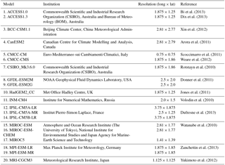
In addition to the regional model results, output from the CMIP5 (https://esgf-node.llnl.gov/search/cmip5/, last access: 4 August 2017) multi-model ensemble was used in this study to elucidate the impact of climate change on compound extreme weather events. A total of 20 CMIP5 models were selected in this study, and the list of models is shown in Table 1. Variables used in this study mainly include daily maximum near-surface air temperature, daily precipitation, daily mean near-surface wind speed, and daily mean 500 hPa wind speed, and the data were interpolated to a spatial resolution of 2∘ × 2∘. Three periods were selected with two periods that overlap in part with that of the regional simulations (1991–2010 as a historical period and 2041–2060 in RCP8.5), and an additional period extending to the end of this century (2081–2100).
The Air Quality System (AQS) dataset (downloaded from https://www.epa.gov/aqs, last access: 8 June 2017) was used in this study to evaluate how well the WRF-Chem model performs in simulating ozone concentrations, particularly high ozone concentrations that are more strongly related to extreme weather events. The locations of observation stations in AQS are shown in Fig. 1 and overlaid on nine climate regions in the US (Karl and Koss, 1984). For evaluation of simulated extreme weather events, the NCEP North American Regional Reanalysis (Mesinger et al., 2005) dataset was used.
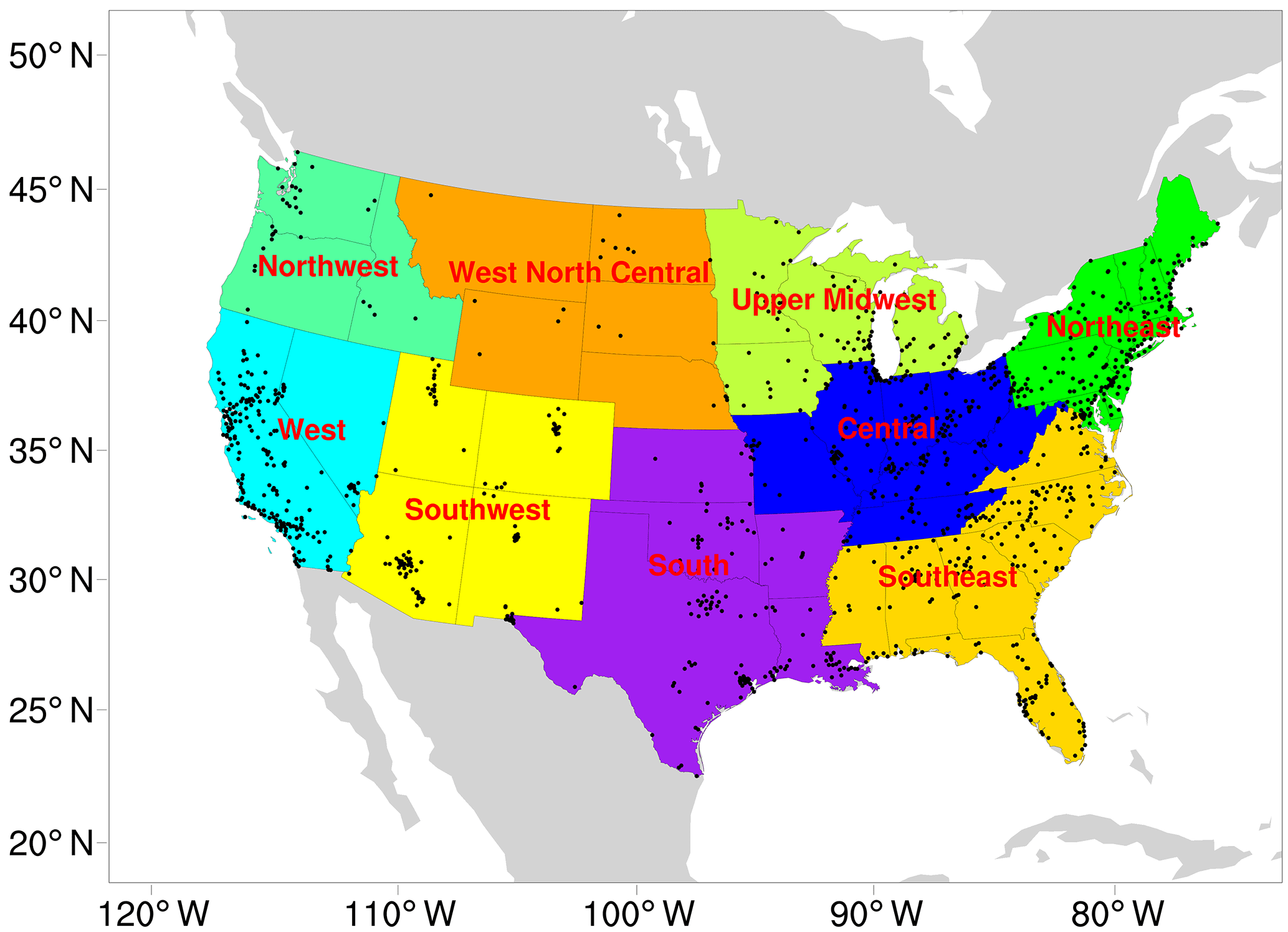
Figure 1The WRF-Chem simulation domain and climate regions in the US. The red points (∼ 1200) represent the observation stations of O3 in AQS.
3.1 Evaluation of extreme weather events
Two types of extreme weather events including heat waves and atmospheric stagnation, as well as their compound events, were investigated, considering their close relationship with ozone pollution (Hou and Wu, 2016). A heat wave is defined to occur when daily maximum 2 m air temperature exceeds a certain threshold continuously for 3 days or more. The threshold is set as the 97.5th percentile of the historical period (2001–2010 for WRF-Chem and 1991–2010 for CMIP5 in this study) and is location dependent to take into account the wide-ranging characteristics of different regions (Gao et al., 2012; Meehl and Tebaldi, 2004). An atmospheric stagnation day is defined to occur when daily mean 10 m wind speed, daily mean 500 hPa wind speed, and daily total precipitation are less than 20 % of the climatological mean condition (2001–2010 for WRF-Chem in this study) (Horton et al., 2014; Hou and Wu, 2016). A compound event occurs when both heat wave and atmospheric stagnation occur simultaneously on the same day. For each grid, the same threshold determined for the present period is used for the future period to evaluate the future changes.
To evaluate the ability of the regional model to reproduce the extreme weather events, Fig. 2 shows the distribution of the mean number of summer heat wave days, atmospheric stagnation days, and compound event days corresponding to coincidental heat wave and atmospheric stagnation during 2001–2010. Observations based on the NARR dataset and the model results are shown, along with scatter plots comparing the observations and simulations at each NARR grid point over land. Statistical metrics, including mean fractional bias (MFB), mean fractional error (MFE), and correlation coefficient (R), based on the Eqs. (A2), (A3), and (A6) in the Appendix, are shown in the scatter plots.
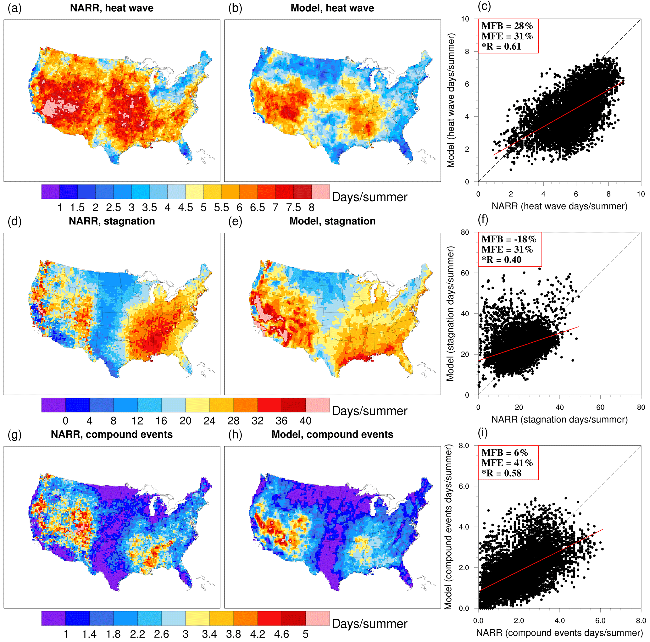
Figure 2Distribution of the mean number of extreme weather days in summer of 2001–2010 from observations (NARR; left panels) and model simulations (middle panels) and scatter plots comparing them at each NARR grid point over land (right panels) for heat wave days (a, b, c), atmospheric stagnation days (d, e, f), and compound event days (g, h, i). The numbers located at the top left of the scatter plots (c, f, i) indicate the statistical metrics including mean fractional bias (MFB), mean fractional error (MFE), and correlation coefficient (R). An r test (α = 0.05) for the linear correlation coefficient was performed and ∗R indicates statistical significance at the 95 % confidence level. The red solid lines in the scatter plots are the linear regression lines, and the black dashed lines are one-to-one reference lines.
The spatial distributions of both heat waves and atmospheric stagnation are generally consistent between NARR and WRF-Chem (top and middle rows in Fig. 2). For example, for heat waves (Fig. 2a, b), the model captures the high frequency of occurrence in the western US and eastern central US albeit with widespread underestimations particularly in the northern US and the central Great Plains. For atmospheric stagnation (Fig. 2d, e), the observed dipole feature of high frequency of occurrence in the western and eastern US, separated by the central Great Plains, is well reproduced by the model but biases in the magnitude are noticeable. To quantitatively evaluate the simulations, the WRF-Chem model results were bilinearly interpolated to the NARR grid suggested by US EPA (2007), and scatter plots were drawn to show the results for all the NARR grid points (Fig. 2c, f). No benchmark is available regarding the statistical metrics for extreme weather events but we adopt the benchmarks widely used in air quality studies. For example, US EPA (2007) suggested 15 %∕35 % (MFB and MFE) for O3 and 50 %∕75 % (MFB and MFE) for PM2.5 species. From this perspective, the MFB and MFE for either heat waves or atmospheric stagnation are within or close to the benchmarks for O3 and well within the benchmarks for PM2.5 species. Moreover, the model results are correlated with NARR, with R equal to 0.61 and 0.40, respectively, for heat waves and atmospheric stagnation and statistically significant at the 95 % confidence level.
The western US receives most of its precipitation in the cold season when the North Pacific jet stream steers storm tracks across the region (Neelin et al., 2013). During summer, the North Pacific subtropical high-pressure center expands and exerts a stronger influence on the western US, increasing the frequency of atmospheric stagnation (Wang and Angell, 1999). Combining the low wind speed and low probability of precipitation during stagnation with low antecedent soil moisture conditions generally prevalent during summer, heat waves can develop to create a maximum center of combined extreme events beyond the coastal mountain ranges of the western US (Zhao and Khalil, 1993). The eastern central US is prone to heat wave and stagnation as a result of the upper level ridge that develops during summer in that region. These climatic conditions give rise to the dipole patterns of maximum heat wave and stagnation in the western and eastern central US. The dipole pattern becomes more obvious and magnified for the compound events because stagnation can promote the development of heat waves, as discussed earlier. For the compound events, the simulation performs well and even better than the metrics of atmospheric stagnation events. The high values in the western and southeastern US, as well as the low values in the central and upper Midwestern US, are reasonably captured by the model, with statistically significant correlation (R=0.58).
Thus, WRF-Chem in general reproduced the spatial patterns and frequency of the extreme weather events including heat waves, atmospheric stagnation, and their compound events well. Although atmospheric stagnation occurs on more than 20 days during the summer in large areas over the western and eastern US, heat waves do not occur for more than 10 days generally; thus the compound events of heat waves and stagnation are rather rare and occur on average for no more than 5 days during summer over the US. In the next section, ozone concentrations during these extreme weather events are analyzed.
3.2 Evaluation of ozone concentrations during extreme weather events
MDA8 ozone is an important variable considering its close relationship with human health (US EPA, 2007) so we focus on the evaluation of MDA8 O3 during summertime. Figure S1 in the Supplement shows the spatial distributions of MDA8 ozone with or without extreme weather events in the WRF-Chem simulations and the NARR-AQS observations. MDA8 ozone with extreme weather events (Fig. S1; left panels) shows a similar increase compared to MDA8 ozone without extreme weather events in both model simulations and observations over the eastern US. On the west coast, the increase is slightly higher in model simulations than in observations. Overall, WRF-Chem reproduced the influence of extreme weather events on enhancing MDA8 ozone over the US well.
From the perspective of public health, the US EPA (2007) recommended attention to ozone values higher than 40 ppbv because the human impact of ozone is small for low ozone concentrations. Thus, we compare the mean ozone concentrations during summer of 2001–2010 between observed data (AQS) and model results for the following three conditions in Fig. 3: (1) days with heat waves but no atmospheric stagnation, (2) days with atmospheric stagnation but no heat waves, and (3) days with compound events (both heat wave and atmospheric stagnation). Thus the first two conditions identify single extreme events and the third condition identifies compound extreme events. We compare observed ozone concentration greater than or equal to 40 ppbv and the simulated ozone concentration corresponding to the same locations of the observations.
As depicted in Fig. 3, WRF-Chem reasonably reproduced the observed ozone concentrations during the extreme weather events, showing statistically significant correlations with the observed AQS data. Moreover, if the benchmark (15 %∕35 % for MFB and MFE and 10 %∕20 % for NMB and NME) suggested by the US EPA (2007) is used as a reference, all the statistical metrics based on evaluation against ozone higher than 40 ppbv in observations are within or much smaller than the benchmarks, illustrating promising ability of WRF-Chem to simulate the ozone concentrations during heat waves, stagnation, and compound events. Even if all ozone values including values below 40 ppbv are considered, the four metrics (MFB, MFE, NMB, and NME) are mostly within the benchmarks and the correlation coefficients between model and observation are only slightly reduced by 0.04, 0.11, and 0.1 for the three types of extreme weather events, respectively, and all values are still statistically significant. However, the general low biases of the simulations are obvious from the regression lines. Ozone concentrations during compound extreme events are clearly shifted to higher values relative to ozone concentrations during single extreme events.

Figure 3Ozone concentration comparison between observations (AQS) and WRF-Chem simulations during heat waves (left), atmospheric stagnation (middle), and compound heat wave and atmospheric stagnation events (right). Metrics shown inside each figure were from Eqs. (A1) to (A6) in the Appendix. An r test (α = 0.05) is performed to test the statistical significance and ∗R indicates statistical significance at the 95 % confidence level. The solid line is the linear regression line, and the dashed line is a one-to-one reference line.
To delve into spatial heterogeneity, ozone concentrations from model and observations for the three types of extreme weather events are shown using box-and-whisker plots in Fig. 4. Considering the detrimental effect on human health when MDA8 ozone concentration exceeds 70 ppbv by National Ambient Air Quality Standards (NAAQS), we evaluate the WRF-Chem simulated ozone concentrations above this particular threshold. We calculated the mean values of MDA8 ozone concentration exceeding 70 ppbv for each type of extreme weather event, and the mean values are marked at the top of each panel in Fig. 4.
The box-and-whisker plots show some unique features in the observations. For example, the mean ozone (red dot) concentrations tend to be slightly higher when heat waves and stagnation occur at the same time, while the mean values are relatively lower during atmospheric stagnation than during heat waves. These are consistent with Fig. 3 in which values are plotted regardless of the regions. This feature was reasonably captured by the model, in particular over regions in the eastern US, such as the Northeast and Southeast. Regarding high ozone concentrations (i.e., values higher than 70 ppbv), the model is skillful in the eastern US with major anthropogenic emissions. The mean bias could be as small as 0.4 ppbv (over the Southeast during heat waves), and mostly within 1 ppbv. However, for some regions, i.e., the West and Southwest, negative biases could reach a few parts per billion by volume; the negative biases in many regions are likely linked to an underestimation of heat wave intensity, which is reflected in the underestimation of heat wave days as shown in Sect. 3.1. Other possible reasons for the negative biases in surface O3 include uncertainties in precursor emissions and boundary conditions as well as overpredictions in precipitation, as reported in Yahya et al. (2017a).
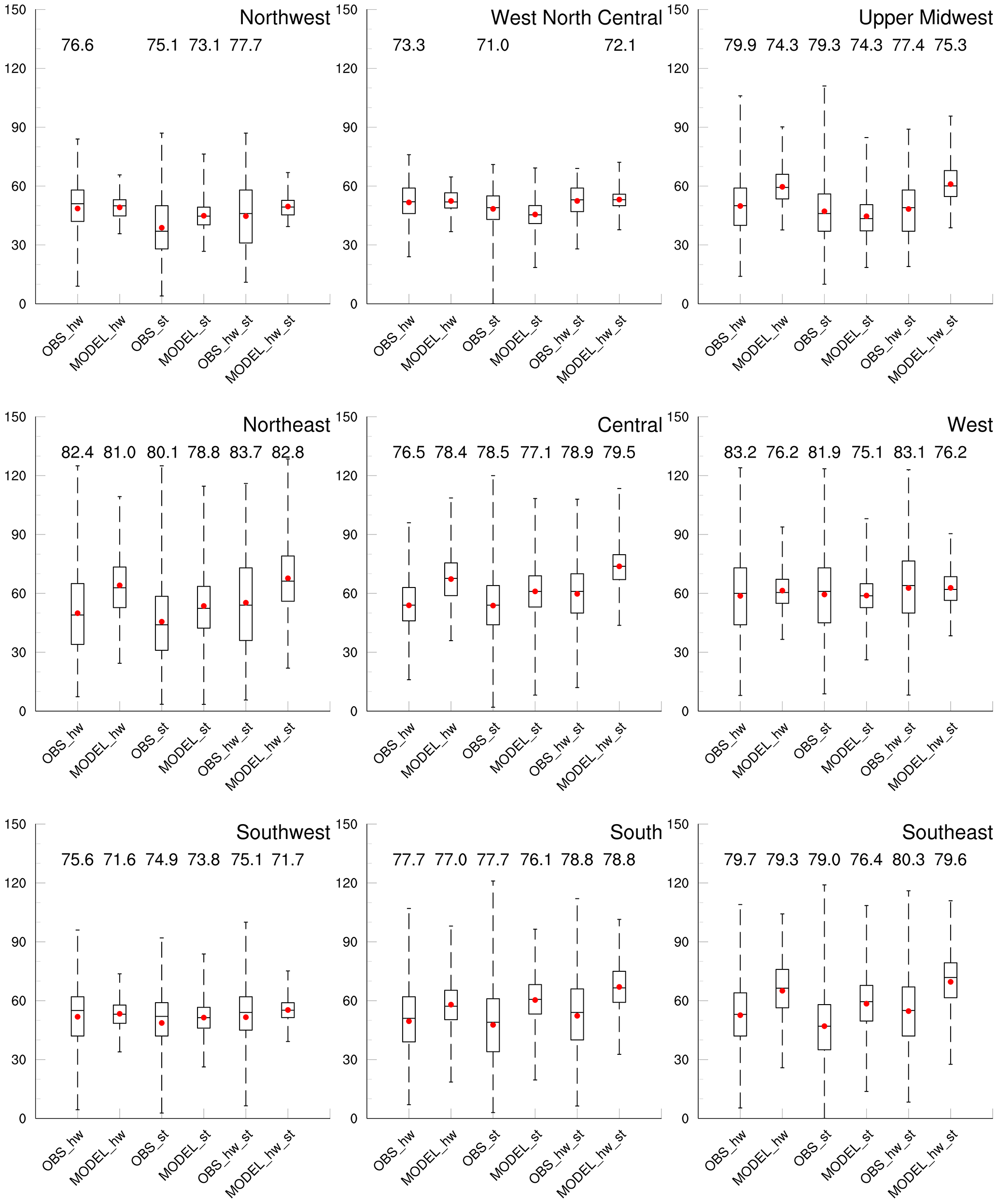
Figure 4MDA8 ozone concentration comparisons during the summer of 2001–2010 in nine climate regions (according to Fig. 1), with box-and-whisker plots showing the minimum, maximum (line end points), 25th percentile, 75th percentile (boxes), medians (black lines), and average (red point) of mean MDA8 ozone from observations (NARR-AQS; with prefix OBS_) and models (WRF-Chem; with prefix MODEL_) during heat waves (with suffix hw), atmospheric stagnation (with suffix st), and compound events of both heat wave and atmospheric stagnation (with suffix of hw_st). The numbers at the top of each panel indicate the average values of MDA8 ozone concentration above the standard (70 ppbv).
To further evaluate the capability of WRF-Chem to model high ozone (beyond 70 ppbv), Fig. S2 displays the interannual variability in high ozone over the US in the WRF-Chem simulations and AQS observations. For observations, the variance of annual mean high ozone was calculated only for grids with more than 5 years of data. Similar to the ozone distribution in Fig. S1, larger values are mainly found on the west coast and in the eastern and central US. Variance over the eastern US in observations is high while WRF-Chem is in general slightly smaller. Considering the total high-ozone episodes in historical periods, the contributions of extreme weather events to the high-ozone episodes are shown in Fig. S3. Only grids having 10 days or more with high ozone are shown to avoid grid cells with very high fractions due to the small number of high-ozone episodes. WRF-Chem simulated a slightly larger fraction on the west coast compared to observations and captured the high fraction in the eastern US well. This feature is similar to the ozone distribution in Fig. S1. Hence overall, WRF-Chem demonstrates a reasonable capability of modeling high-ozone episodes and the contribution of extreme weather events to high-ozone episodes in the US.
4.1 Impacts of single and compound extreme events on ozone concentrations
To investigate the impacts of the extreme weather events on ozone concentrations, we composited the MDA8 ozone concentrations from WRF-Chem for the three types of extreme weather events and periods without any extreme event (non-extreme event) in summer of 2001–2010 using probability density functions (PDFs) shown in Fig. 5.
By comparing the solid lines (extreme event period) and dashed line (non-extreme event period) in Fig. 5, all extreme weather events have positive impacts on ozone, particularly at the high-end tail of the distributions. The difference between ozone concentrations with and without extreme events is statistically significant in all regions at the 95 % confidence level. For regions with mean ozone values exceeding 70 ppbv (numbers shown in Fig. 5), much larger differences are noticeable between the PDFs of extreme and non-extreme periods, with extreme events notably shifting both the low-end and high-end tails towards higher values. These regions include Northeast, Central, South, and West. Conversely, regions such as Northwest, West North Central, and Southwest shows negligible differences between the PDFs. The spatial heterogeneity is closely related to the spatial distribution of emissions in the US, i.e., regions with a larger increase in ozone concentration particularly near the high-end tail (i.e., Northeast, Southeast, Central, Upper Midwest, South, and West) due to extreme weather events are also areas with higher anthropogenic emissions in the US (see also Fig. 3 in Gao et al., 2013). Thus, stronger photochemical reactions in those regions may enhance the effect of extreme weather events on ozone formation.
Now comparing the effects of different types of extreme weather events on ozone concentrations (solid lines of different colors in Fig. 5), the effect of heat waves on ozone formation is generally larger than the effect of atmospheric stagnation, whereas the compound effect is larger than the effect of either type of single extreme weather event. This feature displays similar spatial heterogeneity as discussed above, i.e., the largest impact from the compound effect occurs in South and Central (about half of the compound events leading to MDA8 ozone higher than 70 ppbv), followed by Northeast, South, Upper Midwest, and West (11–28 % compound event days resulting in MDA8 O3 of 70 ppbv or higher), and negligible increase from the compound events for other regions (Northwest, West North Central, and Southwest).
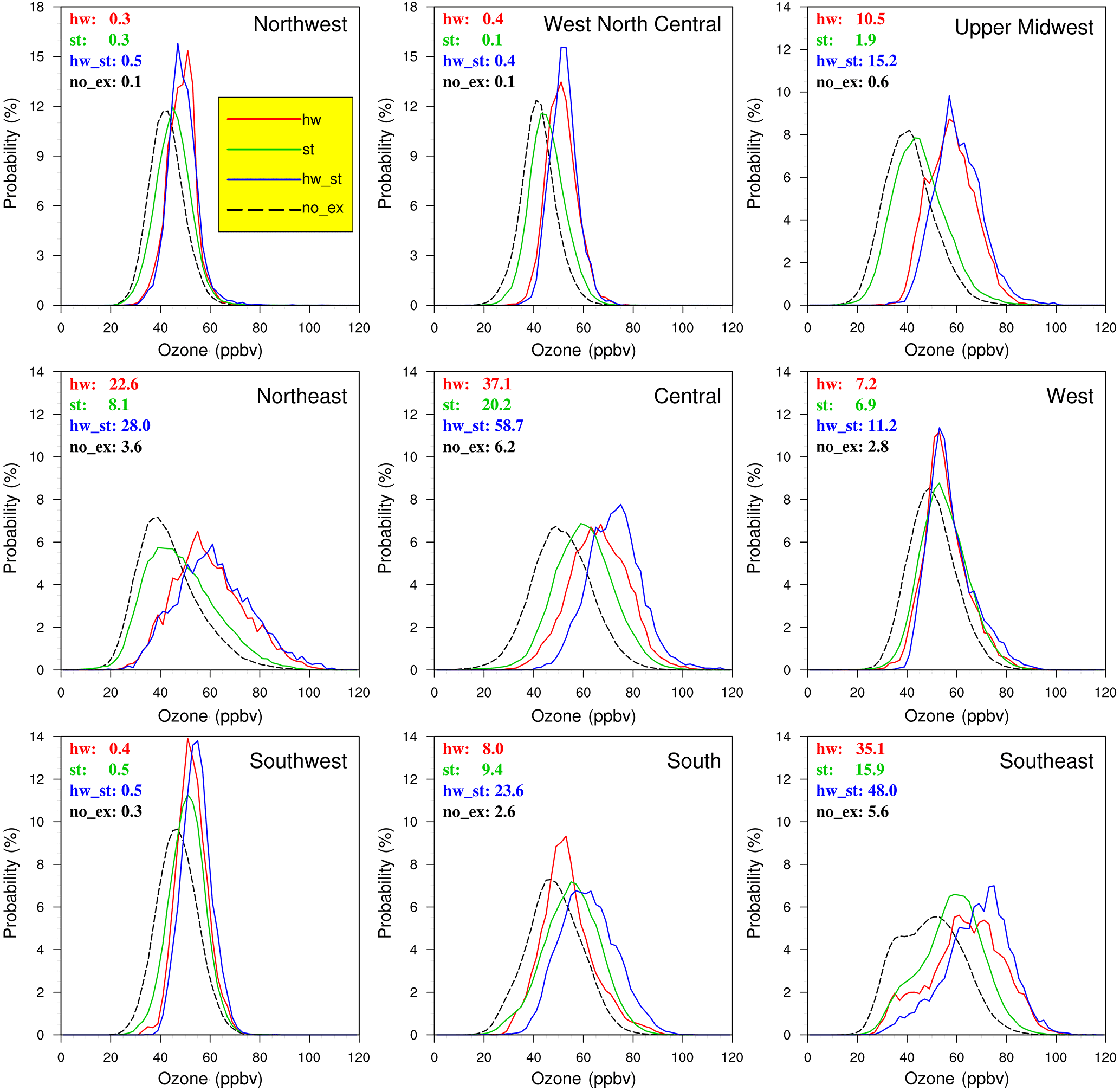
Figure 5Composited probability density distributions of MDA8 ozone simulated by WRF-Chem for three types of extreme weather events (solid lines) and non-extreme event periods (dashed line) during summer of 2001–2010 in nine regions (according to Fig. 1). Each panel includes four numbers in the upper left showing the probability of MDA8 ozone higher than 70 ppbv during extreme weather events for heat waves (hw: red), stagnation (st: green), compound extreme events (hw_st: blue), and non-extreme periods (no_ex: black). Note that all panels except for Northwest and West North Central use the same scale for the y axis.
In addition to the distinguishing impacts extreme events have on ozone relative to non-extreme days, how high the concentration of ozone can reach during extreme events may depend on the intensity of the extreme events and the emissions. Figure 6 shows the correlations between ozone concentration with the daily maximum 2 m temperature during heat waves and 10 m wind speed during atmospheric stagnation events. The correlations between temperature and ozone are positive and statistically significant in areas with high emissions such as Northeast, Central, Upper Midwest, South, and Southeast. For stagnation events, the correlations are statistically significant mainly in South, Southeast, and along the west coast. These correlations between ozone and the intensity of extreme events are consistent with the shift of the high-end tails of the PDFs to higher ozone values, as shown in Fig. 5. In areas with low emissions (e.g., Northwest and West North Central), ozone concentrations are not well correlated with the intensity of extreme events because the production of ozone is limited by the low emissions (Vingarzan, 2004). Hence only the low-end instead of the high-end tails of the PDFs are shifted to higher values in regions with low emissions, and the PDFs on extreme days are noticeably narrower compared to the PDFs on non-extreme days (Fig. 5). As climate change may increase the frequency as well as the intensity of extreme events, ozone concentrations may be affected, regardless of emissions control in the future.
4.2 Impacts of climate change on ozone concentrations
Having investigated the impacts of extreme weather events on ozone concentration, we now focus on how ozone concentrations may change in the future with climate change, changes in biogenic emissions in response to changes in climate, and large anthropogenic emission reductions in the RCP8.5 scenario. Figure 7 shows the spatial variations in ozone concentrations composited during extreme weather events at present (top row) and in the future (bottom row). The spatial features displayed in the top row are in agreement with what have been observed from Fig. 5, showing larger impacts of extreme weather events on ozone formation east of the Rockies for both single extreme events and compound events (Fig. 7a, b, c). Similarly large impacts are also found in California, which are obscured in the regional average shown in Fig. 5. Averaged over the US, MDA8 ozone concentrations increase by 22 and 12 % during heat waves and stagnation events compared to non-heat wave and non-stagnation days. Compound events have a significantly higher impact on ozone compared to the single extreme events, with statistically significant differences of 13 and 16 %, respectively, for heat waves and stagnation (Fig. 7d, e). To understand why compound events have larger impacts than single extreme events, Fig. S4 shows that during compound event days, the daily maximum 2 m temperature is comparable to that during heat waves but 6.27 ∘C higher than that during stagnation events, leading to a 16 % increase in MDA8 O3 during compound events relative to stagnation events. Similarly, the 10 m wind speed during compound events is comparable to that during stagnation events but 1.4 ms−1 weaker than during heat wave days, leading to a 13 % increase in MDA8 O3 relative to heat wave days.
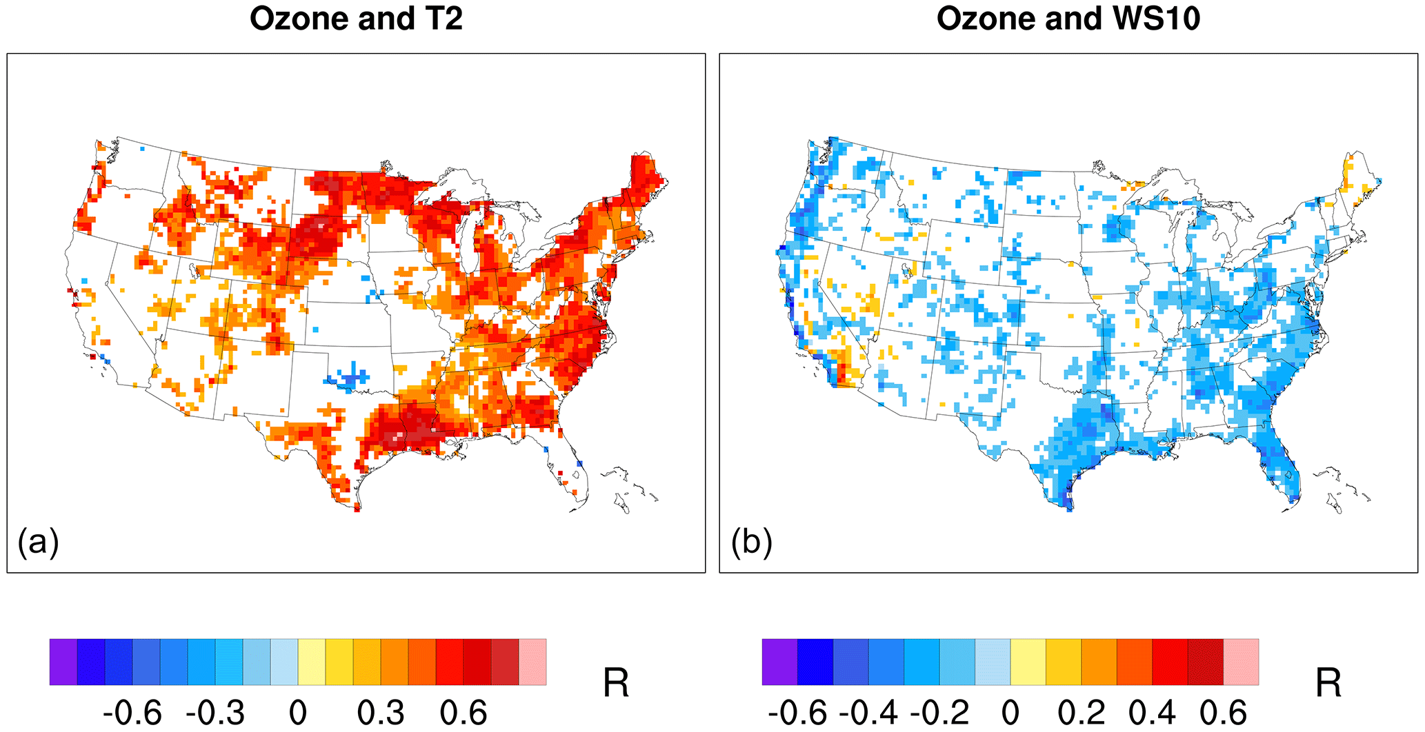
Figure 6Correlation between ozone concentration and (a) daily maximum 2 m temperature (T2) during heat waves and (b) 10 m wind speed (WS10) during atmospheric stagnation in the WRF-Chem simulations. Only values that pass the t test of statistical significance (α = 0.05) are shown in colors.
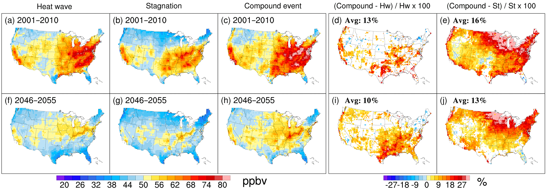
Figure 7Spatial distributions of mean MDA8 ozone concentrations simulated by WRF-Chem for three types of extreme weather event episodes and the relative difference between a compound event and single event during summer in 2001–2010 (a–e) and 2046–2055 under RCP8.5 (f–j). In (d, e, i, j), only values with statistically significant differences (t test: α = 0.05) between the compound effect and single event are shown, and the mean differences are labeled on the top left.
In the future, as anthropogenic emissions are projected to decrease substantially (i.e., Table 2 in Gao et al., 2013), the mean ozone concentration correspondingly decreases during both single extreme events and compound events compared to the present day (i.e., Fig. 7f, g, h vs. Fig. 7a, b, c). However, even with the dramatic anthropogenic emission reduction (i.e., 50 % or more reduction in non-methane volatile organic compounds and nitrogen oxides based on Table 2 in Gao et al., 2013), extreme weather events can still trigger the formation of high ozone concentrations (e.g., in the central eastern US in Fig. 7f, g, h) that reach or exceed the present-day national standard of 70 ppbv. From Fig. S4, the daily maximum 2 m temperature is 5.54 ∘C warmer during compound events than stagnation events, leading to a 13 % increase in MDA8 O3 during compound events relative to stagnation events. Similarly, the 10 m wind speed is 1.28 ms−1 weaker during compound events than heat wave events so MDA8 O3 increases by 10 % during compound events relative to heat wave events in the future. Hence, compound events increase ozone concentrations by 10 and 13 % more than the effect of heat wave only and stagnation only, respectively. These numbers shown in Fig. 7i, j are only 3 % lower than those of the present day (Fig. 7d, e).
Despite dramatic reduction in anthropogenic emissions in the RCP8.5 scenario (Riahi et al., 2011), extreme weather events are still important considerations for air quality and health in the future. This is because both frequency and intensity of extreme events increase in the future, which compensates partly for the effects of reduced emissions. From Fig. S5, heat waves occur on average 13.67 days more and are 0.98 ∘C warmer in the future relative to the present, with most of the increase occurring in the western US. There is no increase in the number of stagnation days in the future when averaged over the US (Fig. S5), and the change in wind speed during stagnation is also negligible (Fig. S6). However, the daily maximum 2 m temperature is 1.42 ∘C warmer during stagnation events in the future compared to the present (Fig. S5). Lastly, compound events occur on average 4.91 days more often, with temperature 1.25 ∘C warmer in the future compared to the present (Fig. S5). Hence the increase in the number of heat waves and the warmer temperature during heat waves as well as stagnation events increase their individual and compound effects on ozone concentrations in the future. These motivate analysis of changes in extreme events in the future using a multi-model ensemble for more robust results.
To provide further insight into future changes in ozone concentration, we analyzed changes in extreme weather events using the multi-model ensemble of CMIP5 data. Using CMIP5 data complements our analysis of the WRF-Chem simulations in two ways. First, CMIP5 model outputs are available for a continuous period through 2100. We analyzed three time periods, each 20 years long, for 1991–2010 as a historical period, and 2041–2060 and 2081–2100 in RCP8.5 as future periods. Extending the analysis period from 10 years for the regional climate simulations to 20 years for CMIP5 allows for a more statistically robust analysis of extreme events. The added period of the late century, 2081–2100, will elucidate how extreme weather events evolve with continuous warming. Second, we extended our analysis using CMIP5 data to the entire Northern Hemisphere starting from 20∘ N. The inclusion of other continents such as Europe and China provides useful information for how extreme weather events may change in densely populated regions, with potential impacts on air quality and health. Analysis of the CMIP5 mean extreme event days over the US shows that in general, the CMIP5 mean has spatial patterns comparable to those of the observations and WRF-Chem simulations but it has a much lower number of extreme event days, especially for stagnation and compound events (not shown). The CMIP5 mean projected changes in extreme event days also show spatial patterns comparable to those of WRF-Chem over the US, but again, the magnitudes of change are much smaller (not shown). Analysis of the CMIP5 projections of extreme event changes is important to provide a multi-model context of uncertainty.
The summer mean number of days at present (1991–2010) and changes in future (2041–2060, 2081–2010) for heat waves, atmospheric stagnation, and compound events are shown in Fig. 8. For robust comparisons between future and present climate, both model agreement and significance are considered, as adopted by previous studies (Gao et al., 2014; Seager et al., 2013; Tebaldi et al., 2011). A total of 20 models were selected (listed in Table 1), and values at any grid cell are considered to have agreement if more than 70 % of the models agree with the CMIP5 mean on the sign of the change. Once agreement is established, statistical significance is tested over the grid cells, and the values at any grid cell are statistically significant if at least half of the CMIP5 models show statistically significant changes (t test, α = 0.05). After the tests, most of the grid cells showing model agreement also passed the statistical significance test; blue dots indicate grid cells with no significant changes of extreme weather events. Three major continents were selected for analysis and the results are summarized in Table 2.
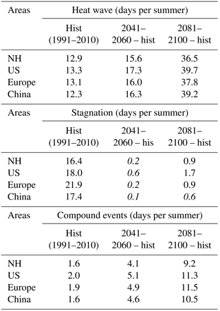
As shown in Fig. 8 and Table 2, at present (Fig. 8a, d, g), the mean annual numbers of heat waves, atmospheric stagnation, and compound events are 12.9, 16.4, and 1.6, respectively. In the future, there are robust increases in heat wave days worldwide, consistent with previous studies (Sillmann et al., 2013), with a mean increase around 200 % by the end of this century. The changes in atmospheric stagnation are in general smaller than the changes in heat waves; however, large increases can also be found in some areas such as the western US. This is in contrast with the insignificant change in stagnation days from the WRF-Chem simulation (Fig. S5), demonstrating the importance of using a multi-model ensemble and investigating changes not just in the mid-century but further towards the end of the century when climate change signals become more prominent (Fig. 8e, f). The overall increase in stagnation events is on average 1 day per summer in the future over the Northern Hemisphere for atmospheric stagnation by the end of this century. Moreover, it is obvious that compound events show more dominant increases than stagnation events, with 2 days or less at present on average, but more than 10 days on average in the US, Europe, and China. Since we have demonstrated that compound events have a larger impact on ozone than single extreme events (Fig. 5), the large increase in compound event days suggests that they will be important considerations for projecting high-ozone episodes.
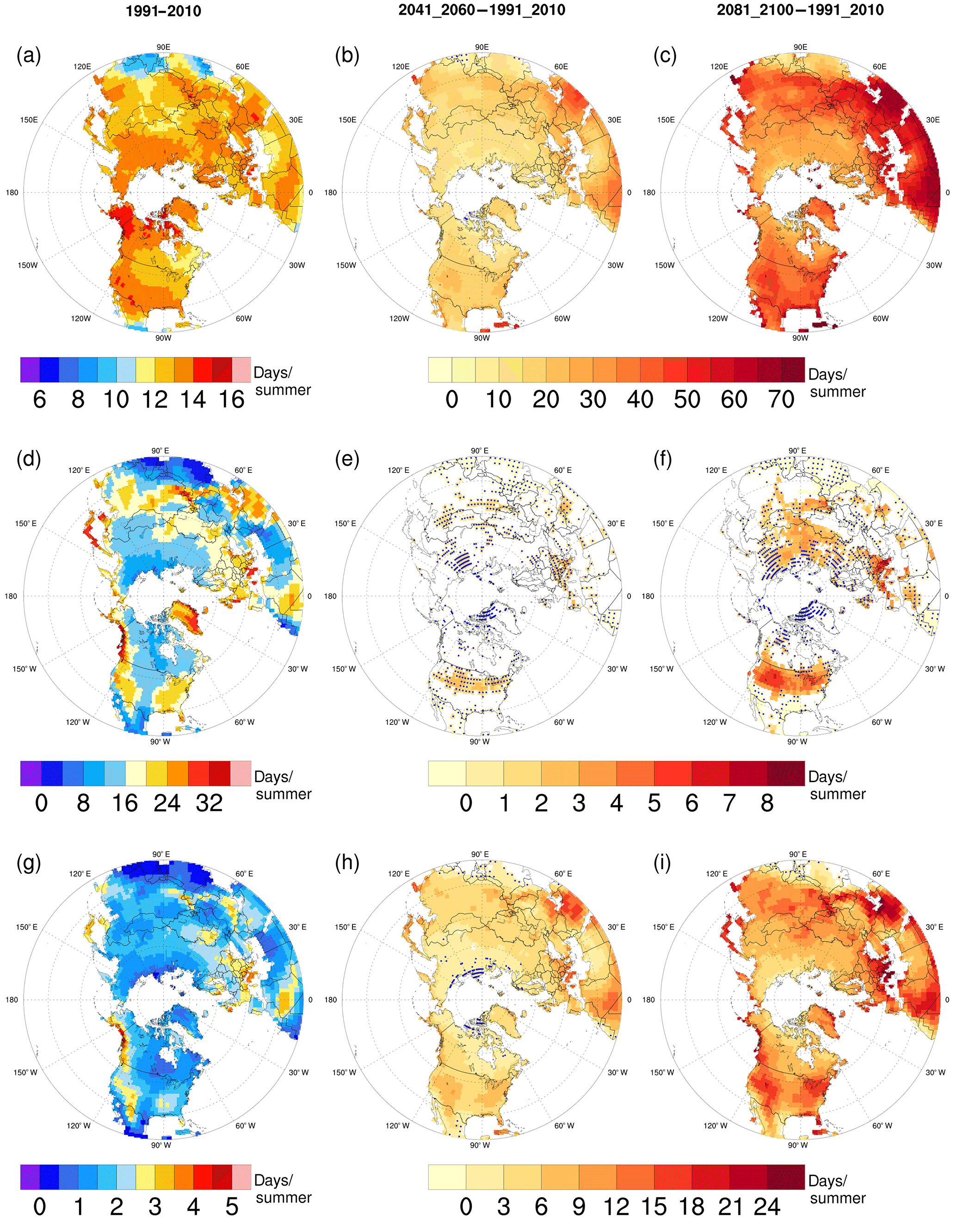
Figure 8Spatial distribution of historical (left column) and future changes in the mid-century (second column) and end of century (third column) in the number of extreme weather days per summer for heat waves (a–c), atmospheric stagnation (d–f), and compound events (g–i) from CMIP5 over land in the Northern Hemisphere north of 20∘ N. For the future changes, only grids showing model agreement are shown, with blue dots representing values with no statistical significance.
As discussed in Sect. 4, both the frequency and intensity of extreme events have important effects on ozone concentrations. From Fig. S7, the intensity of heat waves is projected to increase with time throughout the 21st century as warming increases. Both the WRF-Chem and CMIP5 results show a larger increase in heat wave intensity in the western US. During stagnation and compound events, the daily maximum 2 m temperature also increases with time. Consistent with WRF-Chem results (Fig. S6), CMIP5 also shows negligible changes in wind speed during atmospheric stagnation and compound events, but a decrease during heat waves (Fig. S8), further enhancing the effect on ozone formation.
Table 2Average number of days of extreme weather event episodes in summer of 1991–2010, 2041–2060, and 2081–2100, along with the future increase over the Northern Hemisphere (NH) and three regions including the United States (US), Europe, and China. A statistical significance test was applied using a t test (α = 0.05), and values with no statistical significance are italicized.
The regional model WRF-Chem version 3.6.1 has been used to downscale simulations from the CESM_NCSU global model. The regional model reproduced the frequency of extreme weather events, including heat waves, atmospheric stagnation, and their compound events, and the ozone concentration during these extreme weather events at present well, compared to observations. Through comparison of ozone concentrations during extreme weather events and non-extreme events, we established statistically significant higher ozone concentrations during the extreme event period. In particular, compound events yield the highest contribution to high ozone formation, followed in general by heat waves and atmospheric stagnation.
Compound events have larger impacts on ozone than single events because the temperature during compound events is noticeably higher than that during stagnation-only events and the wind speed during compound events is noticeably weaker than during heat-wave-only events. The combination of warmer temperature and weaker winds promotes photochemical reactions that produce high-ozone episodes. Also, importantly, ozone concentrations increase with the intensity of extreme events in regions with high emissions, leading to a shift in the PDFs towards higher ozone values and increasing the frequency of occurrence of high-ozone episodes. In regions with low emissions, extreme events noticeably increase the ozone concentrations at the low-end tails, but the high-end tails are not shifted, leading to narrower PDFs during extreme events relative to non-extreme events.
In the future, under the RCP8.5 scenario, even though large reductions in anthropogenic emissions are projected, extreme weather events can still trigger the formation of higher ozone concentrations. The increase in ozone concentrations during extreme events relative to non-extreme events is comparable in the future as in the present. Furthermore, compound events of heat waves and stagnation continue to have larger impacts on ozone concentrations relative to the single weather extreme events. By utilizing a total of 20 CMIP5 models, we found that under climate warming, more frequent extreme weather events are projected to occur in the middle to end of this century. Among the increases by the end of the century, compound events show a dominantly higher fractional increase by a factor of 4–5, compared to the single events, i.e., heat waves (∼ a factor of 2) or atmospheric stagnation (∼ 14 %), as shown in Table 2.
Since the CMIP5 models do not include detailed atmospheric chemistry, we cannot assess how ozone concentrations may change in the middle to late 21st century. The CMIP5 results indicate robust increases in the frequency and intensity of heat waves and frequency of compound events with higher temperature in the future. While reductions of anthropogenic emissions in the RCP8.5 scenario will likely counter the effects of extreme events on ozone concentrations, the frequency of high ozone concentrations is enhanced by extreme events even in low emission regions (e.g., Northwest) in the present day (Fig. 5). Hence it is likely that high-ozone episodes may still occur in the future due to increases in extreme heat, despite reductions in anthropogenic emissions, with adverse effect to human health.
However, similar to how low emissions constrain the high-end tails of the PDFs of ozone from shifting to very high or extreme ozone concentrations even under extreme weather conditions (e.g., Northwest in Fig. 5), reductions in anthropogenic emissions in the future could reduce or eliminate the occurrence of extreme high-ozone episodes. Hence controlling anthropogenic emissions may be critical for reducing the impacts of extreme events on extreme air quality episodes and associated human health impacts. This may be especially important in regions like China that have experienced severe air pollution in recent decades. More attention to improving projections of compound events and evaluating their impacts on ozone may better constrain the projections of extreme air quality episodes and inform strategies to reduce their detrimental effects on human health now and in the future.
Analysis data used to generate the plots in this paper can be accessed by contacting Yang Gao (yanggao@ouc.edu.cn), and the WRF-Chem model output can be accessed by contacting Yang Zhang (yzhang9@ncsu.edu).
Metrics for model performance evaluation used in this study include BIAS (mean bias), NMB (normalized mean bias, percent), NME (normal mean error, percent), MFB (mean fractional bias, percent), MFE (mean fractional error percent), and R (correlation coefficient). Calculations of these metrics are shown below in Eqs. (A1)–(A5), where N is the number of sample size, and MODEL and OBS represent the corresponding value in model simulations and observations (AQS sites or reanalysis data), respectively. As low OBS values can amplify the metrics, a cutoff of 40 or 60 ppbv of ozone is suggested in evaluation for ozone. Benchmarks of MFB and MFE for O3 are 15 and 35 %, and of NMB and NME for O3 are 10 and 20 % (US EPA, 2007).
The supplement related to this article is available online at: https://doi.org/10.5194/acp-18-9861-2018-supplement.
YG and LRL came up with the original ideas of investigating the compound effect on ozone pollution, JZ conducted all the analyses, KL and JF helped on the discussion and interpretation of the analysis, and YZ and KW were in charge of the WRF-Chem simulations and data process. All the authors contributed to the writing of the paper.
The authors declare that they have no conflict of interest.
This research was supported under assistance agreement no.
RD835871 by the U.S. Environmental Protection Agency to Yale University
through the SEARCH (Solutions for Energy, AiR, Climate, and Health) project
that supported L. Ruby Leung, Yang Zhang, and Kai Wang, and by grants from the
National Key Project of MOST (2017YFC0209801), National Natural Science
Foundation of China (41705124), and the Fundamental Research Funds for the
Central Universities that supported Junxi Zhang, Yang Gao, Kun Luo, and Jianren Fan. It
has not been formally reviewed by the EPA. The views expressed in this document
are solely those of The SEARCH Center and do not necessarily reflect those
of the agency. The EPA does not endorse any products or commercial services
mentioned in this publication. PNNL is operated for the DOE by the Battelle Memorial
Institute under contract DE-AC05-76RL01830. We thank Khairunnisa Yahya, a
former graduate student of the Air Quality Forecasting Laboratory at NCSU,
for conducting the WRF-Chem simulations used in this work. We acknowledge the
World Climate Research Programme's Working Group on Coupled Modelling, which
is responsible for CMIP, and we thank the climate modeling groups for
producing and making available their model output.
Edited by: Qiang Zhang
Reviewed by: two anonymous referees
Agrawal, M., Singh, B., Rajput, M., Marshall, F., and Bell, J. N. B.: Effect of air pollution on peri-urban agriculture: a case study, Environ. Pollut., 126, 323–329, 2003.
Arora, V., Scinocca, J., Boer, G., Christian, J., Denman, K., Flato, G., Kharin, V., Lee, W., and Merryfield, W.: Carbon emission limits required to satisfy future representative concentration pathways of greenhouse gases, Geophys. Res. Lett., 38, 387–404, 2011.
Bi, D., Dix, M., Marsland, S. J., O'Farrell, S., Rashid, H., Uotila, P., Hirst, A., Kowalczyk, E., Golebiewski, M., and Sullivan, A.: The ACCESS coupled model: description, control climate and evaluation, Aust. Meteorol. Oceanogr. J., 63, 41–64, 2013.
Diffenbaugh, N. S. and Giorgi, F.: Climate change hotspots in the CMIP5 global climate model ensemble, Clim. Change, 114, 813–822, 2012.
Dix, M., Vohralik, P., Bi, D., Rashid, H., Marsland, S., O'Farrell, S., Uotila, P., Hirst, T., Kowalczyk, E., and Sullivan, A.: The ACCESS coupled model: documentation of core CMIP5 simulations and initial results, Aust. Meteorol. Oceanogr. J., 63, 83–99, 2013.
Donner, L. J., Wyman, B. L., Hemler, R. S., Horowitz, L. W., Ming, Y., Zhao, M., Golaz, J.-C., Ginoux, P., Lin, S.-J., and Schwarzkopf, M. D.: The dynamical core, physical parameterizations, and basic simulation characteristics of the atmospheric component AM3 of the GFDL global coupled model CM3, J. Climate, 24, 3484–3519, 2011.
Dufresne, J.-L., Foujols, M.-A., Denvil, S., Caubel, A., Marti, O., Aumont, O., Balkanski, Y., Bekki, S., Bellenger, H., and Benshila, R.: Climate change projections using the IPSL-CM5 Earth System Model: from CMIP3 to CMIP5, Clim. Dynam., 40, 2123–2165, 2013.
Filleul, L., Cassadou, S., Medina, S., Fabres, P., Lefranc, A., Eilstein, D., Le Tertre, A., Pascal, L., Chardon, B., Blanchard, M., Declercq, C., Jusot, J. F., Prouvost, H., and Ledrans, M.: The relation between temperature, ozone, and mortality in nine french cities during the heat wave of 2003, Environ. Health Persp., 114, 1344–1347, 2006.
Fiore, A. M., Naik, V., and Leibensperger, E. M.: Air Quality and Climate Connections, J. Air Waste Manage., 65, 645–685, 2015.
Flynn, J., Lefer, B., Rappengluck, B., Leuchner, M., Perna, R., Dibb, J., Ziemba, L., Anderson, C., Stutz, J., Brune, W., Ren, X. R., Mao, J. Q., Luke, W., Olson, J., Chen, G., and Crawford, J.: Impact of clouds and aerosols on ozone production in Southeast Texas, Atmos. Environ., 44, 4126–4133, 2010.
Gantt, B., He, J., Zhang, X., Zhang, Y., and Nenes, A.: Incorporation of advanced aerosol activation treatments into CESM/CAM5: model evaluation and impacts on aerosol indirect effects, Atmos. Chem. Phys., 14, 7485–7497, https://doi.org/10.5194/acp-14-7485-2014, 2014.
Gao, Y., Fu, J. S., Drake, J. B., Liu, Y., and Lamarque, J. F.: Projected changes of extreme weather events in the eastern United States based on a high resolution climate modeling system, Environ. Res. Lett., 7, 044025, https://doi.org/10.1088/1748-9326/7/4/044025, 2012.
Gao, Y., Fu, J. S., Drake, J. B., Lamarque, J.-F., and Liu, Y.: The impact of emission and climate change on ozone in the United States under representative concentration pathways (RCPs), Atmos. Chem. Phys., 13, 9607–9621, https://doi.org/10.5194/acp-13-9607-2013, 2013.
Gao, Y., Leung, L. R., Lu, J., Liu, Y., Huang, M. Y., and Qian, Y.: Robust spring drying in the southwestern U. S. and seasonal migration of wet/dry patterns in a warmer climate, Geophys. Res. Lett., 41, 1745–1751, 2014.
Glotfelty, T. and Zhang, Y.: Impact of future climate policy scenarios on air quality and aerosol-cloud interactions using an advanced version of CESM/CAM5: Part II. Future trend analysis and impacts of projected anthropogenic emissions, Atmos. Environ., 152, 531–552, 2016.
Glotfelty, T., He, J., and Zhang, Y.: Impact of future climate policy scenarios on air quality and aerosol-cloud interactions using an advanced version of CESM/CAM5: Part I. model evaluation for the current decadal simulations, Atmos. Environ., 152, 222–239, 2017.
Gryparis, A., Forsberg, B., Katsouyanni, K., Analitis, A., Touloumi, G., Schwartz, J., Samoli, E., Medina, S., Anderson, H. R., Niciu, E. M., Wichmann, H. E., Kriz, B., Kosnik, M., Skorkovsky, J., Vonk, J. M., and Dortbudak, Z.: Acute effects of ozone on mortality from the ”Air pollution and health: A European approach” project, Am. J. Resp. Crit. Care, 170, 1080–1087, 2004.
Guenther, A., Karl, T., Harley, P., Wiedinmyer, C., Palmer, P. I., and Geron, C.: Estimates of global terrestrial isoprene emissions using MEGAN (Model of Emissions of Gases and Aerosols from Nature), Atmos. Chem. Phys., 6, 3181–3210, https://doi.org/10.5194/acp-6-3181-2006, 2006.
He, J. and Zhang, Y.: Improvement and further development in CESM/CAM5: gas-phase chemistry and inorganic aerosol treatments, Atmos. Chem. Phys., 14, 9171–9200, https://doi.org/10.5194/acp-14-9171-2014, 2014.
Horton, D. E., Skinner, C. B., Singh, D., and Diffenbaugh, N. S.: Occurrence and persistence of future atmospheric stagnation events, Nat. Clim. Change, 4, 698–703, 2014.
Hou, P. and Wu, S. L.: Long-term Changes in Extreme Air Pollution Meteorology and the Implications for Air Quality, Sci Rep-Uk, 6, 23792, 2016.
Jacob, D. J. and Winner, D. A.: Effect of climate change on air quality, Atmos. Environ., 43, 51–63, 2009.
Jones, C. D., Hughes, J. K., Bellouin, N., Hardiman, S. C., Jones, G. S., Knight, J., Liddicoat, S., O'Connor, F. M., Andres, R. J., Bell, C., Boo, K.-O., Bozzo, A., Butchart, N., Cadule, P., Corbin, K. D., Doutriaux-Boucher, M., Friedlingstein, P., Gornall, J., Gray, L., Halloran, P. R., Hurtt, G., Ingram, W. J., Lamarque, J.-F., Law, R. M., Meinshausen, M., Osprey, S., Palin, E. J., Parsons Chini, L., Raddatz, T., Sanderson, M. G., Sellar, A. A., Schurer, A., Valdes, P., Wood, N., Woodward, S., Yoshioka, M., and Zerroukat, M.: The HadGEM2-ES implementation of CMIP5 centennial simulations, Geosci. Model Dev., 4, 543–570, https://doi.org/10.5194/gmd-4-543-2011, 2011.
Karl, T. and Koss, W. J.: Regional and national monthly, seasonal, and annual temperature weighted by area, 1895–1983, 1984.
Kharin, V. V., Zwiers, F. W., Zhang, X., and Wehner, M.: Changes in temperature and precipitation extremes in the CMIP5 ensemble, Clim. Change, 119, 345–357, 2013.
Leonard, M., Westra, S., Phatak, A., Lambert, M., van den Hurk, B., McInnes, K., Risbey, J., Schuster, S., Jakob, D., and Stafford-Smith, M.: A compound event framework for understanding extreme impacts, Wiley Interdisciplinary Reviews: Clim. Change, 5, 113–128, 2014.
Leung, L. R. and Gustafson, W. I.: Potential regional climate change and implications to US air quality, Geophys. Res. Lett., 32, 367–384, 2005.
Meehl, G. A. and Tebaldi, C.: More intense, more frequent, and longer lasting heat waves in the 21st century, Science, 305, 994–997, 2004.
Mesinger, F., Dimego, G., Kalnay, E., Shafran, P., Ebisuzaki, W., Jovic, D., Mitchell, K., Berbery, H., Fan, Y., and Higgins, W.: North American Regional Reanalysis: Evaluation Highlights and Early Usage, B. Am. Meteorol. Soc., 87, 561–608, 2005.
Mitchell, J. F.: The “greenhouse” effect and climate change, Rev. Geophys., 27, 115–139, 1989.
Moss, R. H., Edmonds, J. A., Hibbard, K. A., Manning, M. R., Rose, S. K., van Vuuren, D. P., Carter, T. R., Emori, S., Kainuma, M., Kram, T., Meehl, G. A., Mitchell, J. F. B., Nakicenovic, N., Riahi, K., Smith, S. J., Stouffer, R. J., Thomson, A. M., Weyant, J. P., and Wilbanks, T. J.: The next generation of scenarios for climate change research and assessment, Nature, 463, 747–756, 2010.
Neelin, J. D., Langenbrunner, B., Meyerson, J. E., Hall, A., and Berg, N.: California Winter Precipitation Change under Global Warming in the Coupled Model Intercomparison Project Phase 5 Ensemble, J. Climate, 26, 6238–6256, 2013.
Otero, N., Sillmann, J., Schnell, J. L., Rust, H. W., and Butler, T.: Synoptic and meteorological drivers of extreme ozone concentrations over Europe, Environ. Res. Lett., 11, 24005, https://doi.org/10.1088/1748-9326/11/2/024005, 2016.
Placet, M., Mann, C. O., Gilbert, R. O., and Niefer, M. J.: Emissions of ozone precursors from stationary sources: a critical review, Atmos. Environ., 34, 2183–2204, 2000.
Qian, Y., Ghan, S. J., and Leung, L. R.: Downscaling hydroclimatic changes over the Western US based on CAM subgrid scheme and WRF regional climate simulations, Int. J. Climatol., 30, 675–693, 2010.
Riahi, K., Rao, S., Krey, V., Cho, C. H., Chirkov, V., Fischer, G., Kindermann, G., Nakicenovic, N., and Rafaj, P.: RCP 8.5-A scenario of comparatively high greenhouse gas emissions, Clim. Change, 109, 33–57, 2011.
Rotstayn, L. D., Collier, M. A., Dix, M. R., Feng, Y., Gordon, H. B., O'Farrell, S. P., Smith, I. N., and Syktus, J.: Improved simulation of Australian climate and ENSO- related rainfall variability in a global climate model with an interactive aerosol treatment, Int. J. Climatol., 30, 1067–1088, 2010.
Sarwar, G. and Bhave, P. V.: Modeling the effect of chlorine emissions on ozone levels over the eastern United States, J. Appl. Meteorol. Clim., 46, 1009–1019, 2007.
Schimel, D., Glover, D., Melack, J., Beer, R., Myneni, R., Kaufman, Y., Justice, C., and Drummond, J.: Atmospheric Chemistry and Greenhouse Gases, 167–187, 2000.
Scoccimarro, E., Gualdi, S., Bellucci, A., Sanna, A., Giuseppe Fogli, P., Manzini, E., Vichi, M., Oddo, P., and Navarra, A.: Effects of tropical cyclones on ocean heat transport in a high-resolution coupled general circulation model, J. Climate, 24, 4368–4384, 2011.
Seager, R., Ting, M. F., Li, C. H., Naik, N., Cook, B., Nakamura, J., and Liu, H. B.: Projections of declining surface-water availability for the southwestern United States, Nat. Clim. Change, 3, 482–486, 2013.
Seneviratne, S. I., Nicholls, N., Easterling, D., Goodess, C. M., Kanae, S., Kossin, J., Luo, Y., Marengo, J., McInnes, K., andRahimi, M.: Changes in climate extremes and their impacts on the natural physical environment, in: Managing the Risks of Extreme Events and Disasters to Advance Climate Change Adaptation, edited by: Field, C. B., Barros, V., Stocker, T. F., Qin, D., Dokken, D. J., Ebi, K. L., Mastrandrea, M. D., Mach, K. J., Plattner, G. K., Allen, S. K., Tignor, M., and Midgley, P. M., A Special Report of Working Groups I and II of the Intergovernmental Panel on Climate Change (IPCC), Cambridge University Press, Cambridge, UK, and New York, NY, USA, 109–230, 2012.
Sharma, S., Sharma, P., and Khare, M.: Photo-chemical transport modelling of tropospheric ozone: A review, Atmos. Environ., 159, 34–54, 2017.
Sillmann, J., Kharin, V. V., Zwiers, F. W., Zhang, X., and Bronaugh, D.: Climate extremes indices in the CMIP5 multimodel ensemble: Part 2. Future climate projections, J. Geophys. Res.-Atmos., 118, 2473–2493, 2013.
Souri, A. H., Choi, Y. S., Li, X. S., Kotsakis, A., and Jiang, X.: A 15-year climatology of wind pattern impacts on surface ozone in Houston, Texas, Atmos. Res., 174, 124–134, 2016.
Taylor, K. E., Stouffer, R. J., and Meehl, G. A.: An Overview of Cmip5 and the Experiment Design, B. Am. Meteorol. Soc., 93, 485–498, 2012.
Tebaldi, C., Arblaster, J. M., and Knutti, R.: Mapping model agreement on future climate projections, Geophys. Res. Lett., 38, L23701, https://doi.org/10.1029/2011GL049863, 2011.
US EPA: Guidance on the Use of Models and Other Analyses for Demonstrating Attainment of Air Quality Goals for Ozone, PM2.5. and Regional Haze, EPA-454/B-07e002, 2007.
van Vuuren, D. P., Edmonds, J. Kainuma,, M., Riahi, K., Thomson, A., Hibbard, K., Hurtt, G. C., Kram, T., Krey, V., Lamarque, J. F., Masui, T., Meinshausen, M., Nakicenovic, N., Smith, S. J., and Rose, S. K.: The representative concentration pathways: an overview, Clim. Change, 109, 5–31, 2011.
Vingarzan, R.: A review of surface ozone background levels and trends, Atmos. Environ., 38, 3431–3442, 2004.
Volodin, E., Dianskii, N., and Gusev, A.: Simulating present-day climate with the INMCM4.0 coupled model of the atmospheric and oceanic general circulations. Izvestiya, Atmos. Ocean. Phys., 46, 414–431, 2010.
Wang, J. X. and Angell, J. K.: Air stagnation climatology for the United States, NOAA/Air Resource Laboratory ATLAS(1), 1999.
Watanabe, M., Suzuki, T., O'ishi, R., Komuro, Y., Watanabe, S., Emori, S., Takemura, T., Chikira, M., Ogura, T., and Sekiguchi, M.: Improved climate simulation by MIROC5: mean states, variability, and climate sensitivity, J. Climate, 23, 6312–6335, 2010.
Weare, B. C., Cagnazzo, C., Fogli, P. G., Manzini, E., and Navarra, A.: Madden-Julian Oscillation in a climate model with a well-resolved stratosphere, J. Geophys. Res.-Atmos., 117, D1, https://doi.org/10.1029/2011JD016247, 2012.
Weschler, C. J.: Ozone's impact on public health: Contributions from indoor exposures to ozone and products of ozone-initiated chemistry, Environ. Health. Persp., 114, 1489–1496, 2006.
Xin, X., Wu, T., and Zhang, J.: Introductions to the CMIP5 simulations conducted by the BCC climate system model, Adv. Climate Change Res., 8, 378–382, 2012.
Yahya, K., Wang, K., Campbell, P., Glotfelty, T., He, J., and Zhang, Y.: Decadal evaluation of regional climate, air quality, and their interactions over the continental US and their interactions using WRF/Chem version 3.6.1, Geosci. Model Dev., 9, 671–695, https://doi.org/10.5194/gmd-9-671-2016, 2016.
Yahya, K., Campbell, P., and Zhang, Y.: Decadal application of WRF/chem for regional air quality and climate modeling over the US under the representative concentration pathways scenarios. Part 2: Current vs. future simulations, Atmos. Environ., 152, 584–604, 2017a.
Yahya, K., Wang, K., Campbell, P., Chen, Y., Glotfelty, T., He, J., Pirhalla, M., and Zhang, Y.: Decadal application of WRF/Chem for regional air quality and climate modeling over the US under the representative concentration pathways scenarios. Part 1: Model evaluation and impact of downscaling, Atmos. Environ., 152, 562–583, 2017b.
Yarwood, G., Rao, S., Yocke, M., and Whitten, G.: Updates to the carbon bond chemical mechanism: CB05 final report to the US EPA, RT-0400675, 2841–2842, 2005.
Yukimoto, S., Adachi, Y., Hosaka, M., Sakami, T., Yoshimura, H., Hirabara, M., Tanaka, T. Y., Shindo, E., Tsujino, H., and Deushi, M.: A new global climate model of the Meteorological Research Institute: MRI-CGCM3 – model description and basic performance, J. Meteorol. Soc. JPN Ser. II, 90, 23–64, 2012.
Zanchettin, D., Rubino, A., Matei, D., Bothe, O., and Jungclaus, J.: Multidecadal-to-centennial SST variability in the MPI-ESM simulation ensemble for the last millennium, Clim. Dynam., 40, 1301–1318, 2013.
Zhao, W. N. and Khalil, M. A. K.: The Relationship between Precipitation and Temperature over the Contiguous United-States, J. Climate, 6, 1232–1236, 1993.
Zscheischler, J. and Seneviratne, S. I.: Dependence of drivers affects risks associated with compound events, Sci. Adv., 3, e1700263, https://doi.org/10.1126/sciadv.1700263, 2017.
Zscheischler, J., Michalak, A. M., Schwalm, C., Mahecha, M. D., Huntzinger, D. N., Reichstein, M., Berthier, G., Ciais, P., Cook, R. B., El-Masri, B., Huang, M. Y., Ito, A., Jain, A., King, A., Lei, H. M., Lu, C. Q., Mao, J. F., Peng, S. S., Poulter, B., Ricciuto, D., Shi, X. Y., Tao, B., Tian, H. Q., Viovy, N., Wang, W. L., Wei, Y. X., Yang, J., and Zeng, N.: Impact of large-scale climate extremes on biospheric carbon fluxes: An intercomparison based on MsTMIP data, Global Biogeochem. Cy., 28, 585–600, 2014.
- Abstract
- Introduction
- Model description and configuration
- Evaluation of meteorology and ozone
- Impacts of extreme events and climate change on ozone concentrations
- Changes of extreme weather events in the future by CMIP5
- Conclusions and discussions
- Data availability
- Appendix A: Statistical metrics for evaluating model performance
- Author contributions
- Competing interests
- Acknowledgements
- References
- Supplement