the Creative Commons Attribution 4.0 License.
the Creative Commons Attribution 4.0 License.
 | 11 Jul 2018
Solar “brightening” impact on summer surface ozone between 1990 and 2010 in Europe – a model sensitivity study of the influence of the aerosol–radiation interactions
Emmanouil Oikonomakis
Martin Wild
Giancarlo Ciarelli
Urs Baltensperger
André Stephan Henry Prévôt
Surface solar radiation (SSR) observations have indicated an increasing trend in Europe since the mid-1980s, referred to as solar “brightening”. In this study, we used the regional air quality model, CAMx (Comprehensive Air Quality Model with Extensions) to simulate and quantify, with various sensitivity runs (where the year 2010 served as the base case), the effects of increased radiation between 1990 and 2010 on photolysis rates (with the PHOT1, PHOT2 and PHOT3 scenarios, which represented the radiation in 1990) and biogenic volatile organic compound (BVOC) emissions (with the BIO scenario, which represented the biogenic emissions in 1990), and their consequent impacts on summer surface ozone concentrations over Europe between 1990 and 2010. The PHOT1 and PHOT2 scenarios examined the effect of doubling and tripling the anthropogenic PM2.5 concentrations, respectively, while the PHOT3 investigated the impact of an increase in just the sulfate concentrations by a factor of 3.4 (as in 1990), applied only to the calculation of photolysis rates. In the BIO scenario, we reduced the 2010 SSR by 3 % (keeping plant cover and temperature the same), recalculated the biogenic emissions and repeated the base case simulations with the new biogenic emissions. The impact on photolysis rates for all three scenarios was an increase (in 2010 compared to 1990) of 3–6 % which resulted in daytime (10:00–18:00 Local Mean Time – LMT) mean surface ozone differences of 0.2–0.7 ppb (0.5–1.5 %), with the largest hourly difference rising as high as 4–8 ppb (10–16 %). The effect of changes in BVOC emissions on daytime mean surface ozone was much smaller (up to 0.08 ppb, ∼ 0.2 %), as isoprene and terpene (monoterpene and sesquiterpene) emissions increased only by 2.5–3 and 0.7 %, respectively. Overall, the impact of the SSR changes on surface ozone was greater via the effects on photolysis rates compared to the effects on BVOC emissions, and the sensitivity test of their combined impact (the combination of PHOT3 and BIO is denoted as the COMBO scenario) showed nearly additive effects. In addition, all the sensitivity runs were repeated on a second base case with increased NOx emissions to account for any potential underestimation of modeled ozone production; the results did not change significantly in magnitude, but the spatial coverage of the effects was profoundly extended. Finally, the role of the aerosol–radiation interaction (ARI) changes in the European summer surface ozone trends was suggested to be more important when comparing to the order of magnitude of the ozone trends instead of the total ozone concentrations, indicating a potential partial damping of the effects of ozone precursor emissions' reduction.
- Article
(13507 KB) -
Supplement
(5325 KB) - BibTeX
- EndNote


Solar radiation plays a key role in the atmospheric chemistry by photo-dissociation of gas molecules. Photolysis reactions, which are mainly driven by the ultraviolet part of the spectrum (100–400 nm), have a significant impact on the formation of tropospheric air pollutants like ozone (Madronich and Flocke, 1999; Seinfeld and Pandis, 2016). The photolysis of ozone leads to its self-destruction (R1) and in the presence of water vapor it becomes the main source of hydroxyl radicals (OH) in the troposphere (R2), while the photolysis of NO2 will lead to ozone production via reactions R3 and R4 (Madronich and Flocke, 1999; Monks, 2005):
The photolysis rate coefficient (J) of a gas is wavelength (λ) dependent and is described by the following equation (Madronich and Flocke, 1999):
where F is the solar actinic flux (photons cm−2 s−1 nm−1) which represents the solar radiation that is incident to a volume element, and φ and σ are the quantum yield and absorption cross section (cm2), respectively, of the gas. φ and σ depend on the gaseous species and the air temperature T (K), as well as on air pressure for some species, while F depends on the position of the Sun and the transmissivity of the atmosphere which is mainly influenced by the presence of clouds, aerosols and radiatively active gases (e.g., O2, O3, water vapor) (Wild et al., 2000; Bian and Prather, 2002). Since the atmosphere can be considered as an optical medium, the total light extinction is governed by the optical depth of the clouds (COD), which mainly scatter light, and of the aerosols (AOD), which either scatter or absorb light (aerosol–radiation interactions (ARIs), which are also referred to as direct aerosol effects) depending on their optical properties (Yu et al., 2006; Seinfeld and Pandis, 2016), as well as by the absorption of gases. In addition, aerosols have an indirect influence on the atmospheric transmissivity (aerosol–cloud interactions (ACIs), which are also referred to as indirect aerosol effects) as they play a role in the formation of clouds by serving as cloud condensation nuclei (CCN) and they can also alter the optical properties and lifetime of clouds (Lohmann and Feichter, 2005; Seinfeld and Pandis, 2016). Aerosols are either directly emitted (primary aerosols) by anthropogenic (e.g., industries, heating processes, vehicles, ships, biomass burning) and natural sources (e.g., volcanos, oceans, deserts), or they are formed through chemical reactions (secondary aerosols) of precursor gases, i.e., SO2, NH3, nitrogen oxides (NOx = NO2 + NO), volatile organic compounds (VOCs) (Fuzzi et al., 2015; Seinfeld and Pandis, 2016). Hence, the human activities can affect the incoming solar radiation by influencing the aerosol loading and radiatively active gas concentrations in the atmosphere.
The multi-decadal changes in aerosol concentrations in the 20th century are considered to be responsible for the changes in surface solar radiation (SSR) in several areas in western Europe and North America. There was a decrease in the SSR between the 1950s and mid-1980s (referred to as solar “dimming”) due to increased industrial and urban production of aerosols, followed by an increase in the SSR since the mid-1980s (referred to as solar “brightening”) when air quality regulations were imposed (Stanhill and Cohen, 2001; Wild et al., 2005; Streets et al., 2006; Ohmura, 2009; Wild, 2009, 2012; Allen et al., 2013; Imamovic et al., 2016). Moreover, extraterrestrial changes or changes in radiatively active gases were ruled out as potential drivers of the solar dimming and brightening (Kvalevåg and Myhre, 2007; Wild, 2009). On the other hand, there are studies arguing that these changes in SSR, especially in pristine or remote areas, were mainly driven by natural changes in cloud cover and/or cloud properties (Dutton et al., 2006; Long et al., 2009; Augustine and Dutton, 2013; Stanhill et al., 2014). However, for Europe, several studies have reported either no statistically significant trends in cloud cover since 1990 or no strong evidence that changes in cloud cover were mainly responsible for the observed SSR trends (Norris and Wild, 2007; Sanchez-Lorenzo et al., 2009, 2012, 2017a; Vetter and Wechsung, 2015). Furthermore, other studies that focused on Europe pointed to aerosols, and especially the ARI, as the main driver for the brightening since the mid-1980s (Ruckstuhl et al., 2008, 2010; Ruckstuhl and Norris, 2009; Folini and Wild, 2011; Sanchez-Lorenzo and Wild, 2012; Wang et al., 2012a; Cherian et al., 2014; Nabat et al., 2014; Turnock et al., 2015; Manara et al., 2016). The relative contribution of clouds and aerosols to the SSR trends might also have a seasonal and spatial dependence, which could be related to changes in large-scale atmospheric circulation patterns like the North Atlantic Oscillation (Stjern et al., 2009; Chiacchio and Wild, 2010; Chiacchio et al., 2011; Parding et al., 2016) or can also depend on the method of study, e.g., surface measurements, satellite observations, SSR proxies like sunshine duration (Sanchez-Lorenzo et al., 2008, 2017b). In addition, it is not clear yet if and to what extent aerosol–cloud interactions influenced the SSR trends in Europe since the mid-1980s (Wild, 2009; Ruckstuhl et al., 2010; Boers et al., 2017).
Tropospheric ozone in Europe has either not decreased as much as expected or even increased in spite of large reductions of precursor emissions since the 1990s (Wilson et al., 2012; Aksoyoglu et al., 2014; Colette et al., 2016). In addition to precursor emissions, European ozone concentrations might also be affected by the hemispheric baseline ozone and changes in photochemical activity (Ordóñez et al., 2005; Andreani-Aksoyoglu et al., 2008). The radiative impact of aerosols on photochemistry and tropospheric ozone over Europe has been examined in several studies (Real and Sartelet, 2011; Forkel et al., 2012, 2015; Kushta et al., 2014; Makar et al., 2015a; San José et al., 2015; Xing et al., 2015a; Mailler et al., 2016). Real and Sartelet (2011) used an offline model (where meteorology and chemistry are decoupled) and performed simulations with and without ARI. They reported that the photolysis rates at the ground level were reduced in the summer, due to the ARI, by 10–14 %, which led to an average surface ozone reduction of 3 and up to 8 % in more polluted areas. A different approach was followed by Xing et al. (2015a, b) to investigate and quantify the impact of multi-decadal ARI changes on surface ozone between 1990 and 2010 over the Northern Hemisphere, by using an online-coupled model. For Europe, they reported a total average increase of 0.3 and up to 3 % for more polluted days over the 21 years when they included the ARI (compared to the no-feedback case). In other words, they suggested that higher AOD (and thus larger ARI) led to higher ozone concentrations due to an increase of atmospheric vertical stability (lower planetary boundary layer (PBL) height) as a result of the ARI surface cooling and above-PBL warming, which resulted in an increase of ozone formation by the accumulation of pollutants close to the surface. This feedback overcompensated for the decreased photolysis rates (due to solar radiation reduction by ARI), although increased photolysis rates do not always lead to higher ozone production (as discussed above), but they can also lead to higher ozone destruction in NOx-limited environments (Bian et al., 2003).
On the other hand, other modeling studies for different summer periods and regions (US and Europe) showed that the influence of ARI on ozone varies spatially, leading to either ozone enhancement or reduction depending on the local meteorological and chemical conditions (Forkel et al., 2012, 2015; Hogrefe et al., 2015; Kong et al., 2015; Makar et al., 2015a; Wang et al., 2015). Moreover, they showed that the impact on ozone (both enhancement and reduction) was even stronger when the ACI were also taken into account. In addition, Forkel et al. (2012) suggested that the spatial patterns of changes in meteorological features due to the aerosol effects should not be taken as a general feature, because they will depend on the prevailing meteorological conditions. Makar et al. (2015a, b) further pointed out that the modeling results of ACI on weather (and consequently on chemistry) will vary based on the model parameterization when comparing the no-feedback case (some models use a “no aerosol” atmosphere while others use different simple parameterizations for aerosol radiative properties and CCN formation) with the one including the ACI. Overall, the research about the aerosol radiative effects (especially the ACI) and their implementation in the online-coupled models to consistently simulate their feedbacks on meteorology and chemistry is still going on, along with the efforts to overcome the problems of high computational demand (Zhang, 2008; Baklanov et al., 2014).
The focus of this study was to investigate the impact of changes in solar radiation in Europe between 1990 and 2010 on summer surface ozone with the following main differences from pre-existing studies. First, we used an offline model, thus excluding ACI, following suggestions from several studies that the ARI was the main driver for the brightening in Europe during the period 1990–2010. In this way, we also excluded the meteorological feedbacks on chemistry due to ARI, emphasizing the more direct and less uncertain impact of ARI on chemistry via the photolysis rates, compared to the more uncertain meteorology–chemistry interactions in the online-coupled models as discussed above. Second, we designed specific sensitivity tests to simulate, as consistently as possible, the observed changes in AOD and SSR in Europe between 1990 and 2010, which is different from the general “switch on/off” ARI approach. Third, we modeled and compared only the initial (1990) and final year (2010) of the studied period using same model input (i.e., the one of 2010; thus, the actual year 1990 was not simulated to avoid the effects from emissions and meteorology, but rather the AOD and SSR conditions representative of the year 1990 were used; see Sect. 2.3) to isolate the influence of ARI on ozone from other factors. Furthermore, this approach is unaffected by any potential masking of the effects of ARI on ozone from interannual variability of key ozone influencing factors (such as meteorology, emissions and boundary conditions), compared to multi-year (with “switch on/off” ARI) simulation studies. Fourth, we included and investigated for the first time (to the best of our knowledge) the impact on biogenic emissions and their effects on ozone. The methods and design of the aforementioned sensitivity tests are described in Sect. 2, accompanied by a particulate matter (PM) trend analysis and discussion (that the model runs were based on) in Sect. 3. The model results are presented and discussed in Sect. 4. Finally, the conclusions are summarized in Sect. 5.
2.1 Model Setup
We used the offline (i.e., the meteorology is prescribed) regional air quality model, CAMx (Comprehensive Air Quality Model with Extensions; http://www.camx.com, last access: 2 July 2018) version 6.30. We modeled the summer season (June, July, August – JJA) in 2010 plus the last 2 weeks of May which were used as spin-up time. The model domain had a horizontal resolution of 0.250∘ × 0.125∘ and covered all of Europe from 15∘ W to 35∘ E and 35∘ N to 70∘ N. The vertical extension was up to 460 hPa using 14 sigma layers. The thickness of the first layer was ∼ 20 m but its modeled values corresponded to ∼ 10 m, as the concentrations are calculated at the midpoint of each layer. We used the CB6r2 (Carbon Bond mechanism, version 6, revision 2; Hildebrandt Ruiz and Yarwood, 2013) gas-phase mechanism, and we simulated the PM concentrations using a static two-mode (fine/coarse) scheme for the aerosol size distribution. For the inorganic thermodynamics and gas–aerosol partitioning calculations, the ISORROPIA scheme (Nenes et al., 1998, 1999) was used, while for the calculations of the organic aerosol concentrations we used the SOAP model (Strader et al., 1999). The dry deposition was calculated according to the scheme of Zhang et al. (2003). The MOZART (Model of Ozone and Related Chemical Tracers) global model data for 2010 (Horowitz et al., 2003) served as initial and boundary conditions for the chemical species. The MOZART data had a time resolution of 6 h and were interpolated to the size and resolution of our grid using the CAMx preprocessor MOZART2CAMx (Ramboll Environ, 2016). The full-science tropospheric ultraviolet and visible (TUV) radiation model (NCAR, 2011) is used as a preprocessor to provide CAMx with clear-sky photolysis rates, where a climatological aerosol profile determined by Elterman (1968) is used. Then, these rates are internally adjusted in CAMx every hour for clouds and aerosols as well as for pressure and temperature using a fast in-line version of TUV (Emery et al., 2010; Ramboll Environ, 2016). The internal adjustment for clouds and aerosols inside CAMx is performed in two steps. First, the clear-sky radiative transfer calculations with in-line TUV are repeated inside CAMx. In the second step, the radiative transfer calculations are repeated including the impact of clouds and aerosols (simulated by CAMx). A ratio of cloudy- (and aerosols) to clear-sky solar radiation is derived by the aforementioned two-step radiative transfer calculations in CAMx. This ratio is then applied to the clear-sky photolysis rates and SSR which were calculated by the full-science TUV preprocessor at the beginning. This internal adjustment (i.e., in-line TUV) is carried out only for a single representative wavelength (350 nm), as tests against the full-science TUV indicated a difference smaller than 1 % in the ratio of cloudy- to clear-sky solar actinic flux for a variety of cloudy conditions (Emery et al., 2010). Inside CAMx, the COD is calculated for each model grid cell based on the approach of Genio et al. (1996) and Voulgarakis et al. (2009), while the dry extinction efficiency of the aerosol species, which is needed for the calculation of the AOD, as well as the single-scattering albedo (SSA) were provided by Takemura et al. (2002) for the wavelength of 350 nm (Table S1 in the Supplement). These values of aerosol optical properties were provided for sulfate, organics, soot, total dust and sea salt, and the sulfate values were extended to nitrate and ammonium (Ramboll Environ, 2016). The asymmetry factor for aerosols was set to have a default value of 0.61 regardless of their composition. For clouds, the default values of the asymmetry factor and SSA were 0.85 and 0.99, respectively. In addition, the eight-stream discrete ordinates scheme was used for the radiative transfer calculations compared to the more common (and computationally faster) two-stream delta-Eddington approximation scheme, as the calculations' accuracy increases with the number of streams (Stamnes et al., 1988; Toon et al., 1989). The choice of eight streams has been suggested to offer high accuracy (1 % or better compared to 32 streams) without having a significantly higher computation cost (Petropavlovskikh, 1995). TOMS (Total Ozone Mapping Spectrometer) data, which were provided by NASA (National Aeronautics and Space Administration; ftp://toms.gsfc.nasa.gov/pub/omi/data/, last access: 2 July 2018), were used as input for total ozone column in both TUV and CAMx. In addition, the radiative transfer algorithms of both full-science TUV and CAMx (i.e., in-line TUV) were modified to extract the modeled AOD and SSR data. In other words, both the SSR (used in the photolysis rate calculation) and the photolysis rates were calculated according to the same parameterization that was described above.
The required meteorological input for CAMx was generated by the WRF-ARW (Advanced Research Weather Research and Forecasting model, version 3.7.1; Skamarock et al., 2008). Reanalysis global data, with time resolution of 6 h and horizontal resolution of 0.72∘ × 0.72∘, were provided by ECMWF (European Centre for Medium-Range Weather Forecasts) and served as initial and boundary conditions for WRF. Both CAMx and WRF had the same model domain and horizontal resolution. However, for the WRF runs, 31 vertical layers, up to 100 hPa were used instead of 14, which was the case for the CAMx runs for computational efficiency. More details about the WRF parameterization are provided in Oikonomakis et al. (2018).
For the anthropogenic emissions, we used the TNO-MACC-III emission inventory for 2010. This inventory was provided by the Netherlands Organization for Applied Scientific Research (TNO) and is an extension of the TNO-MACC-II emission inventory (Kuenen et al., 2014). More details about the TNO-MACC-III emission inventory are given in Kuik et al. (2016). The TNO European emission domain is the same as our domain but with a finer horizontal resolution (0.125∘ × 0.0625∘). The mineral dust, sea salt and wildfire emissions are not included in the inventory. However, in the model's initial and boundary conditions, the concentrations of mineral dust and sea salt are included. For the calculation of the biogenic emissions (isoprene, monoterpenes, sesquiterpenes and soil NO), we followed the methods described by Andreani-Aksoyoglu and Keller (1995) using temperature and SSR data from the WRF output (the SSR data from WRF were not used in any calculation in CAMx) as well as land use data from the GlobCover 2005–2006 land use inventory (http://due.esrin.esa.int/page_globcover.php, last access: 2 July 2018) and the United States Geological Survey (USGS). All emissions were injected in the first model layer and were treated as area emissions. A detailed discussion and values of the emissions used in this study are given in Oikonomakis et al. (2018).
2.2 Observations
The European Air Quality Database v7 (AirBase; Mol and de Leeuw, 2005) provided observational surface data for the air pollutant concentrations (http://acm.eionet.europa.eu/databases/, last access: 2 July 2018) with an hourly time resolution, which were used for chemical model evaluation. For a better comparison between the model and the observations, we used only rural background stations due to our grid resolution. Furthermore, we evaluated the daily mean of the chemical species in order to be able to compare our results with other studies (e.g., Bessagnet et al., 2016). More details about the observational data treatment and the statistical methods are described in the model evaluation part of Oikonomakis et al. (2018). Furthermore, PM10 (particles with an aerodynamic diameter, d<10 µm) and PM2.5 (d<2.5 µm) data from the AirBase database as well as from the Swiss National Air Pollution Monitoring Network (NABEL; Empa, 2010) were used for trend analysis. Switzerland and the Netherlands were chosen for the PM trend analysis as they have PM10 data going back to 1990 and 1992, respectively. For Switzerland, the PM10 data until 1997 are actually corrected total suspended particle (TSP) data (Empa, 2010), but they are suitable for PM10 trend analysis (Barmpadimos et al., 2011). Hourly high-quality SSR data from the Baseline Surface Radiation Network (BSRN; König-Langlo et al., 2013) for seven stations were used for model evaluation. An overview of the seven BSRN stations is given in Table S2. Finally, AOD data were retrieved by the Aerosol Robotic Network (AERONET), which is a network of ground-based Sun photometer measurements of aerosol optical properties (Holben et al., 1998; O'Neill et al., 2003). We used level 2.0 (quality assured) data for the 340 nm wavelength band to compare with the respective modeled AOD values. The calibration error of the AOD measurements is of the order of 0.015 (Holben et al., 1998; Eck et al., 1999). Since the temporal resolution of the AOD measurements is not constant (e.g., at specific hours), the calculated daily mean does not correspond to a 24 h time interval but to intra-day time intervals with available measurements. The daily average of the modeled AOD was calculated using only the times of available AOD measurements for each site, for a more consistent comparison between model and observations.
2.3 Model runs
The description of 12 model runs is shown in Table 1. We used two base case scenarios: one with the default parameterization (BASE) and a second one with increased NOx emissions (BASE_NOx) which produced higher ozone concentrations, in order to incorporate any potential underestimation of the ARI effects on ozone due to underestimated modeled ozone production as suggested by Oikonomakis et al. (2018). All sensitivity tests were performed using both base case scenarios (see Table 1).
Table 1Summary of model runs. All runs used the emissions and meteorology of 2010.
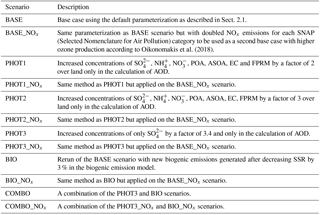
The impact of solar radiation changes due to the ARI on ozone chemistry was investigated via two pathways: (i) via impact on photolysis rates and (ii) via impact on biogenic volatile organic compound (BVOC) emissions. In order to quantify these impacts, we first simulated the summer of 2010, then applied sensitivity tests that would represent the radiation conditions in the summer of 1990 (i.e., different solar radiation due to ARI) and finally compared the two cases. In other words, we used the same meteorology and emissions for both cases (except for the BVOC emission sensitivity tests where we used different BVOC emissions) and we designed special sensitivity tests to isolate and quantify the effect of changes in the ARI between those years on ozone concentrations. Finally, it is noted that the chemistry simulated by CAMx (for any scenario) does not affect the meteorology, as it is prescribed (see Sect. 2.1), and hence the impact of ARI on atmospheric dynamics and other meteorological related effects (e.g., vertical mixing, dry deposition, Xing et al., 2017) are excluded in this study.
2.3.1 Impact via photolysis rates
In order to quantify only the changes in ARI, we had to isolate them from other effects such as the gas–aerosol chemical interactions. For this reason, we modified the radiative transfer algorithm in CAMx (i.e., the in-line version of TUV) by applying an adjustment factor (pf) in the AOD calculation to represent the aerosol concentrations in 1990 but without changing the concentrations themselves and thus avoiding any change due to chemistry. So, the adjusted AOD for N vertical layers and M aerosol species was calculated as shown below:
where μext is the aerosol dry extinction efficiency (see Table S1), f(RH) is the relative humidity (RH) adjustment factor (FLAG, 2000), C is the aerosol species concentration, and Δz is the layer's thickness. Hence, the product pf⋅C represents the PM concentrations in 1990 but purely in AOD calculations in order to generate only AOD, solar radiation and photolysis rates as in 1990. The value of pf for sulfate (), ammonium (), nitrate (), primary organic aerosol (POA), anthropogenic secondary organic aerosol (ASOA), elemental carbon (EC) and fine other primary aerosol (FPRM) varies with the sensitivity test, while there was no adjustment (i.e., pf=1) for biogenic secondary aerosol (BSOA), sodium chloride (NaCl), fine (FCRS) and coarse (CCRS) crustal aerosols, and coarse other primary aerosol (CPRM). We have excluded the natural aerosols (biogenic SOA, sea salt and dust (FCRS + CCRS)) from the AOD adjustment since the anthropogenic aerosol concentration reductions were suggested as a likely explanation for the brightening (see Sect. 1); moreover, no significant change in their contribution to the AOD trends was reported (Streets et al., 2009). Although large natural aerosol contributors like volcanic eruptions (e.g., El Chichón in 1986 and Pinatubo in 1991) can introduce large spikes in the SSR time series, they do not alter the longer-term trends (Wild, 2009). In addition, we also excluded the coarse mode (PM10–PM2.5) of the anthropogenic aerosols from the AOD adjustment, assuming that the fine mode (PM2.5) dominated the decreasing trend of the total aerosol mass (discussed in detail in Sect. 3; Barmpadimos et al., 2012; Tørseth et al., 2012). The pf values 2 and 3 (corresponding to ∼ 50 and 65 % reductions in PM2.5 concentrations, respectively, in 2010 compared to 1990) for the first two sensitivity tests (PHOT1 and PHOT2, respectively, in Table 1), were inferred by a PM trend analysis based on observations (discussed in detail in Sect. 3) and they represent an estimated range of reductions in PM2.5 concentrations between 1990 and 2010 in Europe, i.e., PM2.5_1990 = PM2.5_2010 ⋅ pf. The assumption for PHOT1 and PHOT2 scenarios is that the estimated observed changes in PM2.5 are the same for all species, which does not necessarily correspond to reality as some species decreased more () than others (), while for some others (EC) trends are not known as there were no measurements during the 1990s in Europe (Tørseth et al., 2012). However, sulfate was and still is one of the single most important components that contribute to the total aerosol mass concentration in Europe (Putaud et al., 2010; Tørseth et al., 2012). Moreover, the sulfate measurements started in 1972, so its trends and changes (between −60 and −80 %) are well known for our period of study (Tørseth et al., 2012; Banzhaf et al., 2015; Xing et al., 2015c; Colette et al., 2016) and are within the same range as the changes considered in PHOT1 and PHOT2 scenarios. Therefore, we consider the PHOT1 and PHOT2 scenarios to be good proxies for the purpose of this study, at a regional scale. Furthermore, in order to investigate the impact of sulfate in more detail, we included another sensitivity test (PHOT3 scenario) where we adjusted only the sulfate concentrations in 2010 by a factor of 3.4, which represents approximately a −70 % total change in sulfate concentrations between 1990 and 2010 based on the aforementioned studies. Another aspect to be considered was the anthropogenic aerosols originating directly or indirectly from ship emissions. Since marine emissions were not regulated during 1990–2010 (Eyring et al., 2005; Aksoyoglu et al., 2016), we did not adjust the AOD (i.e., pf=1) over the sea and ocean (for PHOT1, PHOT2 and PHOT3 scenarios), where the contribution of ship emissions to the PM2.5 concentrations is more significant (up to 50 %) compared to continental Europe (up to 10 %) as shown by Aksoyoglu et al. (2016) for the summer of 2006. This way, we expect that the photolysis rate sensitivity tests will represent in general more consistently the AOD conditions of 1990, even though this approach might be conservative as the European maritime AOD trends suggest a decline (significant at the 95 or 99 % level) since the early/mid-1990s (Mishchenko et al., 2007; Cermak et al., 2010; Li et al., 2014a).
2.3.2 Impact via BVOC emissions
We investigated the effect of changes in the solar radiation on biogenic VOC emissions and the subsequent impact on ozone, in two steps. The first step was to generate new biogenic emissions after decreasing the solar radiation input values in the biogenic emission model by 3 % (corresponding to the SSR conditions of 1990), as the observed relative change of SSR in Europe in the summer season between 1990 and 2009 (i.e., the SSR was 3 % lower in 1990 compared to 2009) according to Turnock et al. (2015). These new emissions would correspond to 1990 conditions with respect to the SSR factor; changes in other parameters due to SSR changes, like temperature and photosynthesis as well as diffuse to direct radiation ratio, were not taken into account. The second step was to rerun CAMx with these new biogenic emissions (BIO scenario) and compare with the base case (BASE scenario, Table 1). Finally, we included a scenario (COMBO) with the combined effects of biogenic emissions (BIO scenario) and photolysis rates (PHOT3 scenario; it was chosen as it was considered to be the least uncertain scenario compared to PHOT1 and PHOT2) to assess the overall impact of the ARI changes on surface ozone.
As discussed in Sect. 2.3, the adjustment factor (pf) used in the sensitivity tests represents the total relative change in aerosol concentrations between 1990 and 2010 for the summer season. Although for the SSR such a value was available in the literature (Turnock et al., 2015) for a similar time period (1990–2009) as in this study for the summer season, this was not the case for the total aerosol concentrations. Therefore, we performed a trend analysis to estimate the total relative change of aerosol concentrations for the time period 1990–2010. Several studies report a decreasing trend in both PM10 and PM2.5 concentrations in Europe since the 1990s, following the reductions in the anthropogenic emissions of PM10, PM2.5 and gas precursors responsible for secondary aerosol formation (EEA, 2014, 2017). Barmpadimos et al. (2012) and Tørseth et al. (2012) suggested that the decreasing trend in PM10 concentrations was dominated by the reductions in the PM2.5 concentrations for the periods 1998–2010 and 2000–2009, respectively, as the aerosol coarse mode (PM10–PM2.5) had either a very small decrease or in some cases even a small increase. Although Wang et al. (2012b) claimed a smaller decrease in PM2.5 than in PM10 during 1992–2009, this could be attributed to the difference in number and type of the sites as discussed by Fuzzi et al. (2015). Hence, for our trend analysis, we assumed that the aerosol coarse mode remained constant throughout the period 1990–2010. Therefore, we subtracted the 2010 aerosol coarse mode from the PM10 concentrations of all years to infer the PM2.5 concentrations' trend, as there are no PM2.5 measurements available for the whole examined period (i.e., from 1990–1992 to 2010), and calculate their total change over the period of study. The adjustment factors (pf) were then based on the total relative changes of the estimated PM2.5 concentrations for the summer season (see Table 2).
Table 2Trends (and their standard errors) and total changes in PM10 concentrations measured at three stations in Switzerland (1990–2010) and at three stations in the Netherlands (1992–2010). The total relative changes in the estimated PM2.5 concentrations are also reported in parentheses. All trends are statistically significant (at the 99 % confidence level).
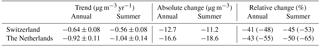
The linear trends were calculated with the Theil–Sen method (Sen, 1968) and their significance was evaluated with the Mann–Kendall test (Mann, 1945; Kendall, 1948). The stations selected for the trend analysis (three for Switzerland and three for the Netherlands) fulfilled the following criteria: (i) they covered the whole period (1990–2010) (Switzerland) or 1992–2010 (the Netherlands) for PM10 data; (ii) they had at least 70 % of daily PM10 and PM2.5 data in each month; and (iii) they had both PM10 and PM2.5 data for 2010 in order to calculate the 2010 aerosol coarse mode (PM10–PM2.5). An overview of the stations is given in Table S3. Regarding the data treatment, the monthly average was calculated initially for each station separately and the 2010 aerosol coarse mode was subtracted to estimate PM2.5 concentrations as discussed above. Then, an average over the stations was taken before the annual (or summer) average was calculated requiring all 12 (or 3) months to be available for a year to be considered in the analysis. The slope of the Theil–Sen trend gave the absolute concentration change per year (µg m−3 yr−1), which was then multiplied by the number of year intervals (number of years − 1) to yield the total absolute change for the respective period. The total relative change was estimated by dividing the total absolute change by the regression value of the respective period's initial year.
The changes in the measured PM10 and estimated PM2.5 concentrations at selected stations over the studied period and the results of the trend analysis are shown in Fig. 1 and Table 2, respectively, for summer as well as for the whole year. A steeper decreasing trend in PM10 concentrations is evident for the Netherlands (−0.92 ± 0.11 µg m−3 yr−1) compared to Switzerland (−0.64 ± 0.08 µg m−3 yr−1), especially in the summer (−1.04 ± 0.14 and −0.56 ± 0.08 µg m−3 yr−1, respectively). The annual total relative change in PM10 concentrations is −43 % for the Netherlands and −41 % for Switzerland. This is in line with the −44 % PM10 change in Europe for the time period 1992–2009 that was reported by Wang et al. (2012b). Our PM10 trend results for Switzerland are also in line with the results (−0.53 and −0.58 µg m−3 yr−1, for annual and summer trends, respectively) reported by Barmpadimos et al. (2011) for the time period 1991–2008; small differences in the trends between the studies are attributed to the inclusion of more sites (with available data later than 1990) in Barmpadimos et al. (2011).
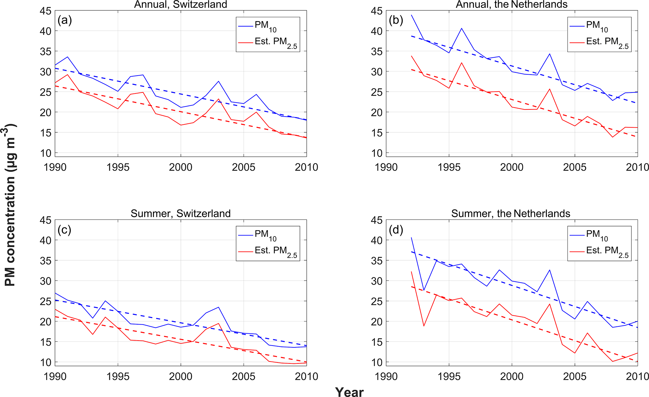
Figure 1Annual (a, b) and summer (c, d) concentrations of PM10 (blue) and PM2.5 (red) measured at three stations in Switzerland (a, c) and at three stations in the Netherlands (b, d) for the period 1990–2010 and 1992–2010, respectively. Dashed lines show the linear regression fit. PM2.5 concentrations were estimated as described in Sect. 3.
4.1 Model evaluation
The model performance evaluation for both WRF and CAMx models was carried out and discussed in detail in Oikonomakis et al. (2018). A summary of the statistical metrics and model performance evaluation is given in Tables 3 and 4, respectively, for the daily mean O3, PM2.5 and PM10 (see also Fig. S1). The model performance for O3 and PM2.5 was satisfactory, as discussed in detail by Oikonomakis et al. (2018). On the other hand, there was a consistent underestimation of PM10 with a mean bias (MB) of −6 µg m−3 and normalized mean bias (NMB) of −33 %. However, the correlation coefficient for the PM10 is 0.5, suggesting that the model can capture the observed PM10 temporal evolution (Fig. S1). Also, since the model performance for PM2.5 is better, this implies that the discrepancy in the PM10 is more likely due to missing emissions in the coarse mode such as sea salt, mineral dust and wildfires (see Sect. 2.1). Even with the inclusion of such emissions, models still have difficulties simulating the PM10 concentrations accurately, as the uncertainties related to these emissions are large and meteorological uncertainties (e.g., in wind speed, vertical mixing) also play an important role (Karamchandani et al., 2017; Solazzo et al., 2017).
Table 3Definition of statistical metrics for model performance evaluation. Mi and Oi stand for modeled and observed values, respectively, and N is the total number of paired values.
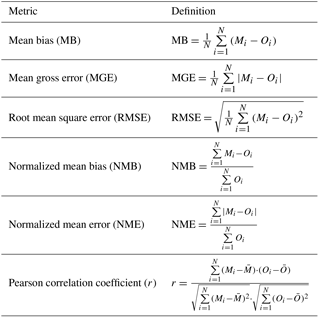
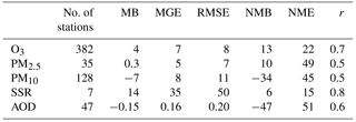
Table 4Statistical summary of model performance evaluation for summer 2010. The units for MB, MGE and RMSE are in ppb for O3, in µg m−3 for PM and in W m−2 for SSR, while the units for NMB and NME are in percent.
The systematic model underestimation of the PM10 concentrations is also evident in the AOD (Table 4), where the model consistently underestimates the AERONET observations (MB of −0.15, MGE of 0.16). Despite this systematic negative bias, the model is able to represent quite accurately the spatial and temporal variability of the observed AOD, indicated by the relatively high correlation (r=0.6) between the model and the observations which is shown in more detail in Fig. S1. Other possible error sources for the modeled AOD could be (i) the simplified treatment of the aerosol size distribution, the optical properties and the mixing state (Curci et al., 2015); (ii) the use of the constant climatological aerosol Elterman (1968) profile for the upper troposphere and stratosphere; (iii) uncertainties in RH and f(RH) for inorganic aerosols; and/or (iv) uncertainties due to grid resolution (horizontal or vertical). Overall, our model AOD discrepancies are within range with other modeling studies (Cesnulyte et al., 2014; Im et al., 2015), where they underline the importance of dust and sea salt treatment in the models.
In the case of SSR, the model performance is better, with a slight overestimation (NMB of 6 %; Table 4). The diurnal and inter-daily variability was captured as well (Figs. 2 and S1; r=0.8). In general, the overestimation of the downward shortwave radiation is a long-standing issue in the models (Wild, 2008; Wild et al., 2013), which indicates that it might be related not only to aerosols but also to other important sources of uncertainty such as parameters related to clouds and water vapor. Since the modeling framework of this study is based on the PM2.5, we believe that the systematic PM10 model bias would not affect the results and conclusions significantly.
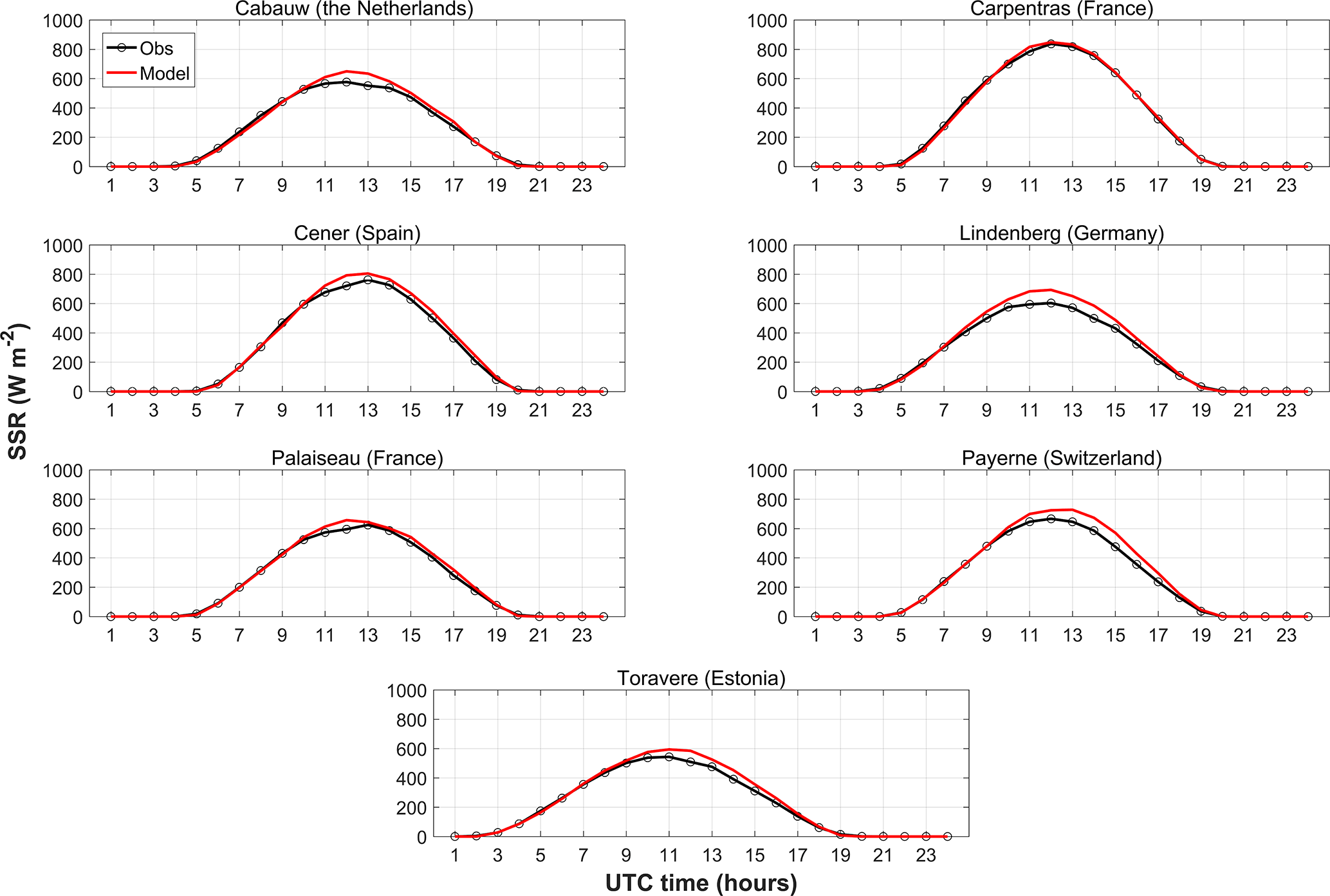
Figure 2Mean diurnal profiles of observed and modeled (BASE scenario) SSR at seven European sites from the BSRN network in summer 2010.
4.2 PM species
The modeled daytime (10:00–18:00 LMT) concentrations of the fine PM species to be adjusted for AOD and SSR calculations are shown in Fig. 3. Sulfate concentrations were predicted to be the highest in summer among all seven species (Fig. 3a) especially over the Mediterranean Sea and southeastern Europe. Although ship emissions are considered to be the main source of elevated sulfate concentrations over the sea, their contribution to the land areas in Southeastern Europe (e.g., Greece and Turkey) is much smaller compared to other emission sources, such as power generation, industries and road transport (Tagaris et al., 2015; Aksoyoglu et al., 2016). Particulate nitrate concentrations, on the other hand, are higher in regions with high NOx and NH3 emissions (around the English Channel, Benelux region, northern Italy). The concentrations of anthropogenic SOA (Fig. 3d) are very low, and the spatial distribution of primary species POA, EC and FPRM is similar to their emission patterns (Fig. 3e–g). The high POA concentrations on the eastern boundary of the model domain are consistent with the summer 2010 Russian wildfires, which influenced mainly the areas around Moscow and to a lesser extent the eastern part of Europe (Mei et al., 2011; Portin et al., 2012; Péré et al., 2015). It is noted that, although wildfire emissions are not included in the model (see Sect. 2.1), they enter the model domain from the model boundaries.
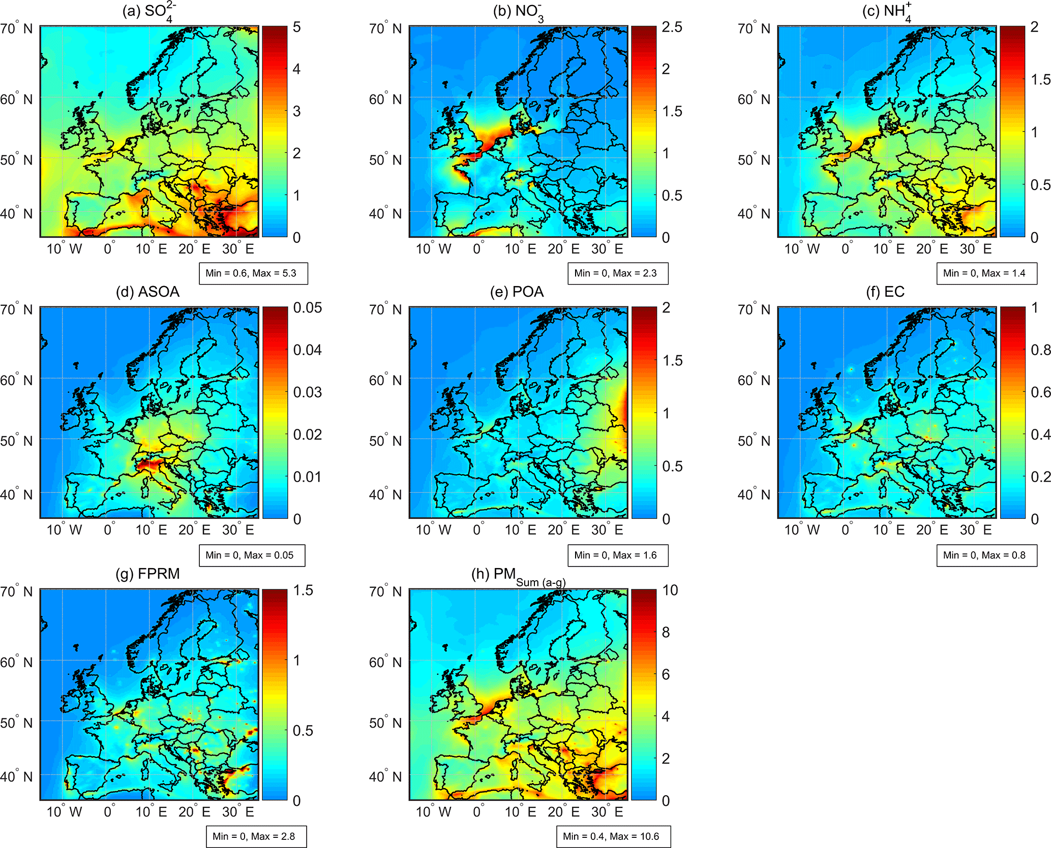
Figure 3Seasonal daytime (10:00−18:00 LMT) mean concentrations (µg m−3) of (a) sulfate (), (b) nitrate (), (c) ammonium (), (d) anthropogenic secondary organic aerosol (ASOA), (e) primary organic aerosol (POA), (f) elemental carbon (EC), (g) fine other primary aerosols (FPRM) and (h) sum of panels (a–g), for the BASE scenario in summer 2010.
4.3 Results of PM adjustment scenarios
4.3.1 Changes in AOD
In this section, the AOD in the base case (BASE) is compared to the AOD after the adjustment of fine PM species to represent the conditions in 1990 (see Table 1 for the adjustment scenarios). The simulated AOD in the base case (Fig. 4a) has a similar spatial distribution over the European domain to the anthropogenic aerosols (see Fig. 3h), although the highest AOD values in the whole grid are in the dust-enriched northwest Africa (in the model, dust is included only in the boundary conditions). The European (i.e., excluding northwest Africa) land (land and marine) grid mean of the AOD is 0.14 (0.13), while in more polluted regions (e.g., Po Valley, Benelux region, western Turkey), the AOD values are as high as 0.20–0.25. The spatial distribution of modeled AOD is in line with modeling results and satellite observations (at around 550 nm) from other studies for different summer periods (Real and Sartelet, 2011; Xing et al., 2015b; Mailler et al., 2016), as well as with the eight-model ensemble results of the PM10 spatial distribution for 2010 by Colette et al. (2017).
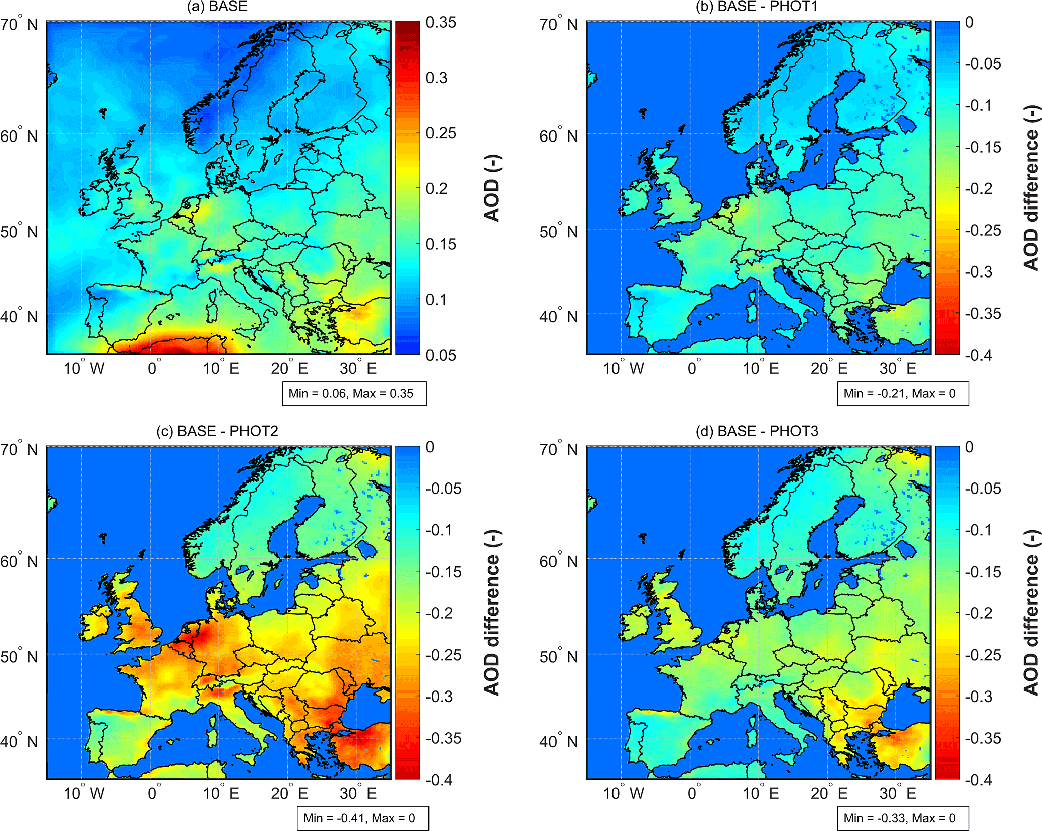
Figure 4Seasonal daytime (10:00−18:00 LMT) mean AOD at 350 nm for the BASE scenario (a) and AOD differences between the BASE scenario and the PHOT1, PHOT2 and PHOT3 scenarios (b–d), respectively, in summer 2010. Note the reversed color order in the color scales of panels (b–d).
The changes in the calculated AOD after the adjustment of the PM species according to the descriptions given in Table 1 are shown in Fig. 4b–d. The largest difference in AOD was obtained with the PHOT2 scenario (Fig. 4c) of up to −0.41, followed by the PHOT3 (Fig. 4d) and PHOT1 scenarios (Fig. 4b) with up to −0.33 and −0.21, respectively. The continental European grid averages for the AOD differences between the base case (BASE) and PHOT1, PHOT2 and PHOT3 scenarios are −0.10, −0.21 and −0.15, respectively. The changes in AOD in all three tests consistently follow the spatial distribution of anthropogenic aerosols (see Fig. 3h), with southwestern and northern Europe having the smallest values due to higher contribution of dust and BSOA, respectively, to aerosol concentrations in these regions (Fig. S2). The spatial distribution of the simulated AOD differences (Fig. 4b–d) is similar to that from the modeled difference in PM10 concentrations between 1990 and 2010 (Colette et al., 2017), supporting the assumptions used in our sensitivity tests. Xing et al. (2015b) reported that the simulated trends of AOD (at 533 nm) in summer in Europe were −0.007 and −0.003 yr−1, for the periods 1990–2000 and 2000–2010, respectively, resulting in −0.1 for the whole period (1990–2010). They also calculated an AOD summer trend of −0.002 to −0.007 yr−1 from the analysis of satellite observations for the period of 2000–2010. Turnock et al. (2015) reported modeled and observed (from AERONET sites) summer AOD (at 440 nm) trends of −0.005 and −0.014 yr−1, respectively, for the period 2000–2009, which are higher than the ones reported by Xing et al. (2015b) probably due to the lower wavelength used by Turnock et al. (2015). This could be an indication that the fine-mode particles were mainly responsible for the decreasing AOD trends, as their scattering efficiency is higher at smaller wavelengths (Seinfeld and Pandis, 2016). Li et al. (2014b) also suggested that the AOD reduction in Europe might have been driven by decreases in the fine-mode particles. The authors reported decreasing trends in the AOD (at 440 nm), as well as in the Ångström exponent (at 440/870 nm), for the vast majority of the European AERONET sites between 2000 and 2013; the largest AOD decrease was observed in western Europe with −0.1 decade−1 (i.e., −0.010 yr−1). Another study by Bin et al. (2017) further supported the conclusions about the AOD decreasing due to the smaller particles. They showed that the AOD (at 555 nm) trend from satellite observations for western Europe in summer was yr−1 between 2001 and 2015. Assuming that the AOD trend between 1990–2000 and 2000–2010 was the same, we estimated the AOD trend in Europe for 1990–2010 to be , −0.010 and −0.008 yr−1 for the PHOT1, PHOT2 and PHOT3 scenarios, respectively. Our results about the change in AOD are in the same range as the other studies, by taking into account that (i) for smaller wavelengths (350 nm in our case and > 440 nm in the aforementioned studies) larger changes are expected due to the higher decreasing trend in the fine-mode particle concentrations as discussed above; (ii) the AOD reduction might have been larger for 1990–2000 than 2000–2010 (Xing et al., 2015b).
4.3.2 Changes in SSR
In this section, the SSR in the base case (BASE) is compared to the SSR after the adjustment of fine PM species to represent the conditions in 1990 (see Table 1 for the adjustment scenarios). The modeled SSR for the base case (BASE) is shown in Fig. 5a. The model captured both the magnitude and the spatial distribution with the south–north latitudinal gradient and the lowest values over the northwest Atlantic Ocean, as also shown by other studies (Forkel et al., 2012, 2015). The average (maximum) differences in SSR over land between the base case (BASE) and PHOT1, PHOT2 and PHOT3 tests are 9 (20), 17 (35) and 11 (26) W m−2, respectively (Fig. 5b–d). Following the same method as for the AOD, we estimated the SSR trend as 0.45, 0.85 and 0.55 W m−2 yr−1 for PHOT1, PHOT2 and PHOT3, respectively. Other studies reported modeled and observed SSR trends within a range of 0.35–0.55 W m−2 yr−1 for different periods between 1986 and 2012 (Norris and Wild, 2007; Allen et al., 2013; Cherian et al., 2014; Nabat et al., 2014; Sanchez-Lorenzo et al., 2015; Turnock et al., 2015). Based on these studies, PHOT1 and PHOT3 are more realistic scenarios than PHOT2 which seems to present a slight overestimation of the ARI changes. Xing et al. (2015a) reported for Europe SSR changes between 1990 and 2010 in the range of 6–18 W m−2 in line with PHOT1 and PHOT3 scenarios (Fig. 5b and d). In general, our simulated AOD and SSR changes between 1990 and 2010 for PHOT1 and PHOT3 scenarios seem to be consistent with respective observed and modeled changes from other studies, while the PHOT2 scenario can be considered rather an upper limit of the ARI changes.
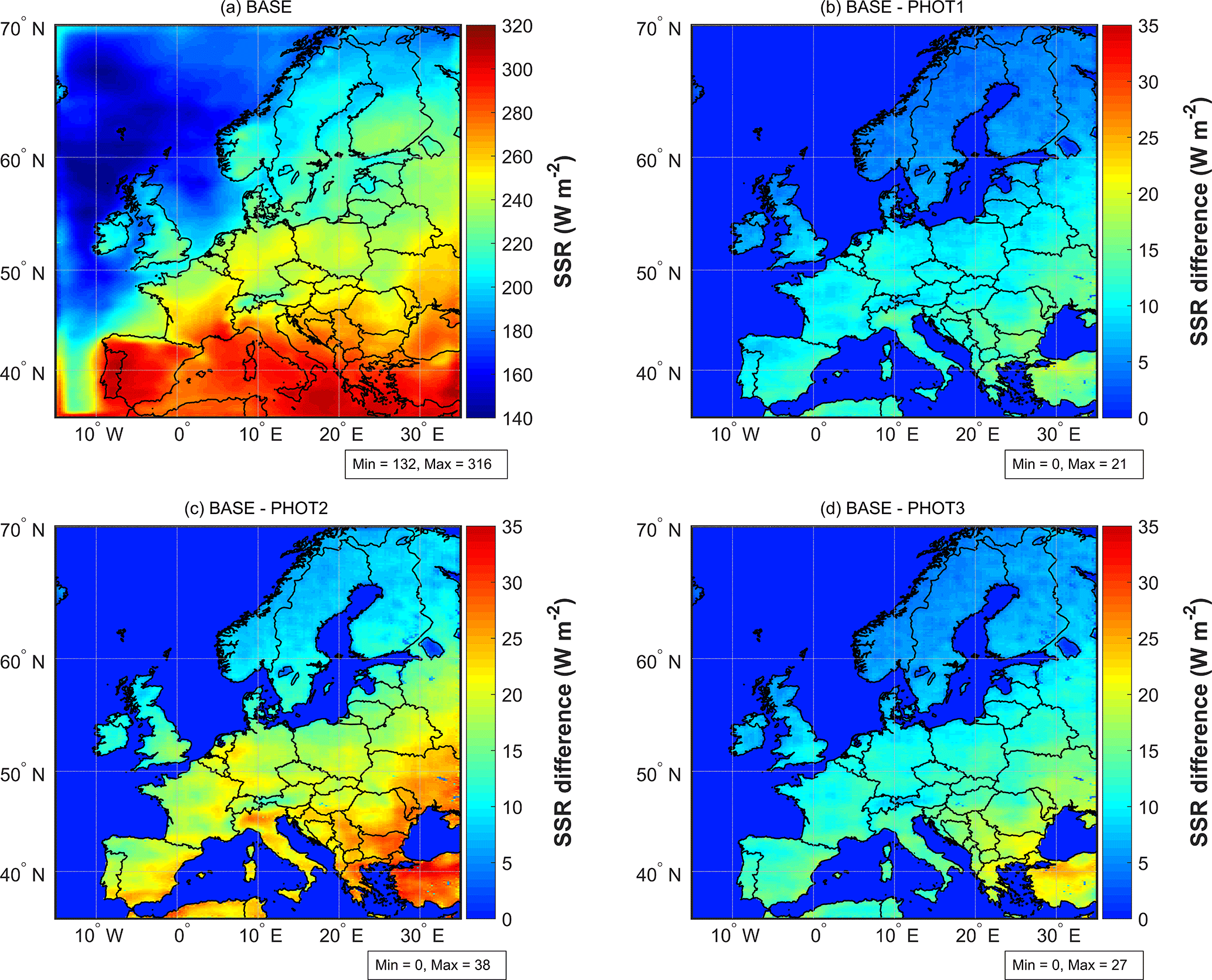
Figure 5Seasonal daily mean SSR for the BASE scenario (a) and SSR differences between the BASE scenario and the PHOT1, PHOT2 and PHOT3 scenarios (b–d), respectively, in summer 2010. Note the different color scale between panel (a) and panels (b–d).
4.4 Effects on ozone via photolysis rates
The simulated (in the base case) ground-level photolysis rate of NO2, J(NO2), consistently follows the south-to-north latitudinal gradient of SSR and temperature, as shown in Fig. 6a. The modeled continental mean absolute (relative) differences in ground-level J(NO2) between the base case (BASE) and PHOT1, PHOT2 and PHOT3 tests are 0.7 (3 %), 1.3 (6 %) and 0.9 (4 %) h−1, respectively (Fig. 6b–d). The spatial distribution and relative changes are the same for the ground-level photolysis rate of O3, J(O3 → O1D), with changes in absolute terms being 0.0015, 0.0029 and 0.0020 h−1, respectively, for PHOT1, PHOT2 and PHOT3 tests (Fig. S3). As discussed in Sect. 1, changes in the photolysis rates will affect the chemical production and destruction of ozone as well as other chemical processes in the troposphere such as the secondary aerosol (SA) formation, which in turn can affect the photolysis rates. This implication, however, is rather small with the change in SA concentration (continental grid mean) between base case (BASE) and PHOT1, PHOT2 scenarios being 0.01 and 0.02 µg m−3, respectively (Figs. S4–S5) or in relative terms 0.3 and 0.6 %, respectively (the respective results for the PHOT3 test are very similar to the ones of the PHOT1 test and are therefore not shown). We conclude that these changes in SA have negligible impact on the photolysis rates. However, the changes in SA might not be negligible if the impact of ARI on meteorology and subsequent effects on chemistry are also taken into account (which is not the case for this study).
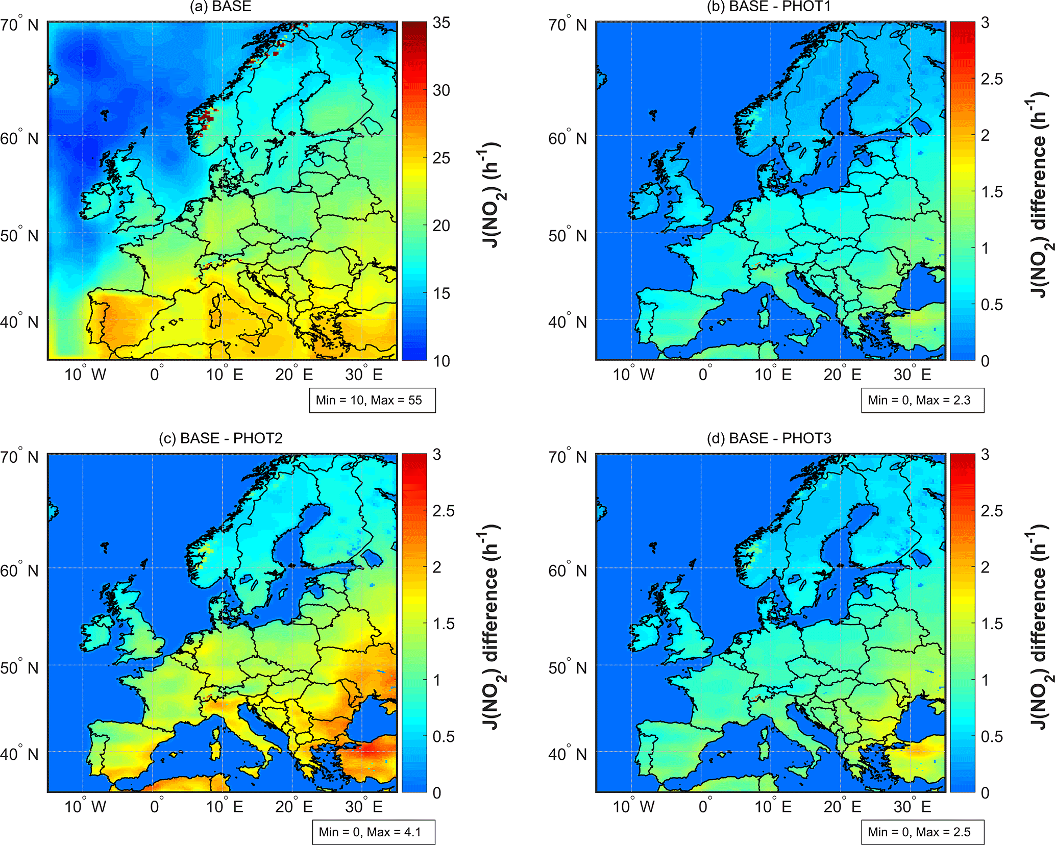
Figure 6Seasonal daytime (10:00−18:00 LMT) mean J(NO2) at ground level for the BASE scenario (a) and J(NO2) differences between the BASE scenario and the PHOT1, PHOT2 and PHOT3 scenarios (b–d), respectively, in summer 2010. Note the different color scale between panel (a) and panels (b–d).
The enhancement of the photolysis rates leads to higher ozone formation especially in regions where there are significant ozone precursor emissions (i.e., central Europe, northern Italy; Fig. 7). The magnitude of the effect of enhanced photolysis rates is, however, rather small on average. The difference in the surface ozone between BASE and PHOT2 scenarios during the daytime (10:00–18:00 LMT) varies between 0.4 and 0.7 ppb (1–1.5 %) over central Europe and up to 1.4 ppb (2.5 %) in the Po Valley, while it is smaller for the other two scenarios (up to 0.7–0.8 ppb, 0.7–1.4 %). However, on an hourly resolution, the largest difference in surface ozone between BASE and PHOT2 scenarios can go up to 8 ppb (16 %) and up to 4 ppb (10 %) for the PHOT1 and PHOT3 scenarios in high-NOx areas on land (Fig. S6).
We repeated similar tests based on a second base case (BASE_NOx) with increased NOx emissions which improved the model performance for ozone production as discussed in Oikonomakis et al. (2018). In the BASE_NOx case, ozone production was higher over a larger area compared to the BASE (see Figs. 7a and 8a). Consequently, the difference in ozone between BASE_NOx and the PHOT1_NOx, PHOT2_NOx and PHOT3_NOx scenarios was more pronounced over a larger area; the magnitude of the impact, however, only slightly increased (Figs. 8 and S6).
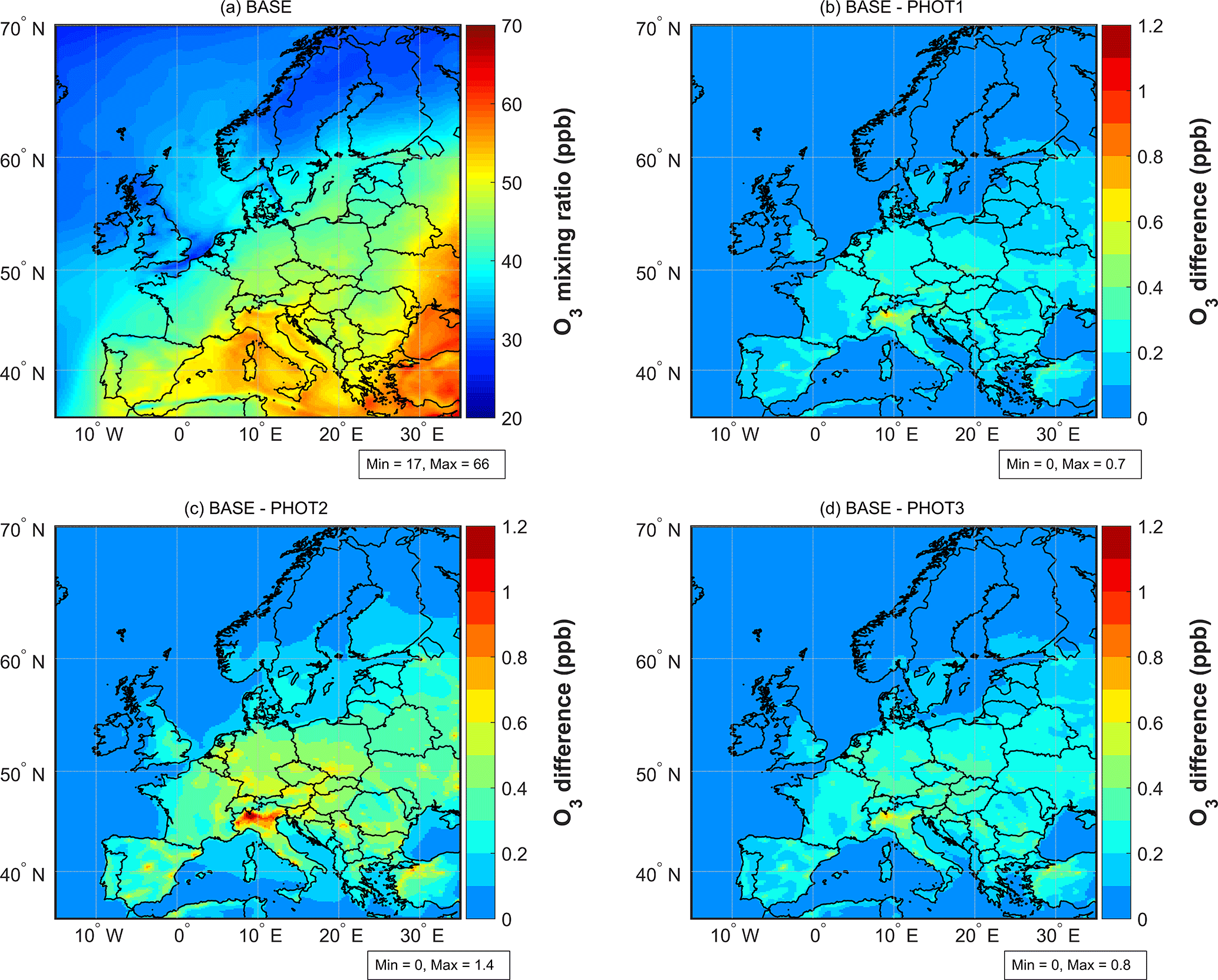
Figure 7Seasonal daytime (10:00−18:00 LMT) mean O3 mixing ratios for the BASE scenario (a) and O3 differences between the BASE scenario and the PHOT1, PHOT2 and PHOT3 scenarios (b–d), respectively, in summer 2010. Note the different color scale between panel (a) and panels (b–d).
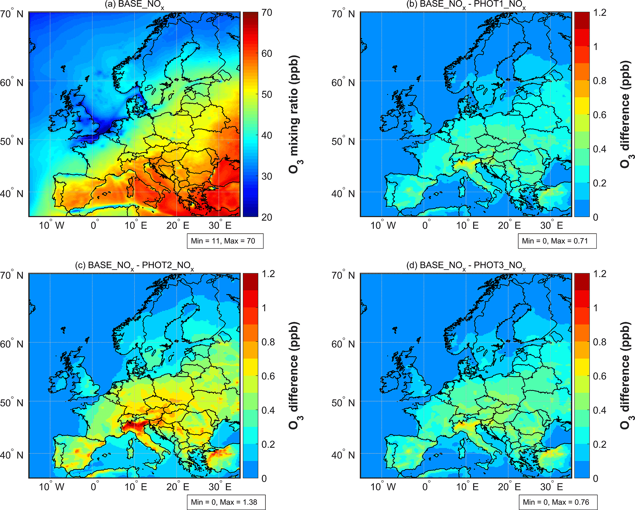
Figure 8Seasonal daytime (10:00–18:00 LMT) mean O3 mixing ratios for the BASE_NOx scenario (a) and O3 differences between the BASE_NOx scenario and the PHOT1_NOx, PHOT2_NOx and PHOT3_NOx scenarios (b–d), respectively, in summer 2010. Note the different color scale between panel (a) and panels (b–d).
We also investigated the impact of ARI changes on daily maximum ozone, but it was higher only by up to ∼ 0.1 ppb (not shown) compared to the daytime (10:00−18:00 LMT) average. Therefore, the ARI did not have a significantly higher impact on daily maximum ozone. The reason is that the daily maximum ozone occurs at a different time (mid-afternoon) than the times the maximum ARI occurs (morning and evening), as also shown in other studies (Xing et al., 2015a, 2017).
4.5 Effects on ozone via BVOC emissions
The response of isoprene emissions (2.5–3 % changes) to SSR changes (3 %) is nearly linear (Fig. 9), in line with the literature (Guenther et al., 2006). On the contrary, terpene (monoterpene and sesquiterpene) emissions are less sensitive to SSR with changes up to 0.7 % (Fig. 9). Nevertheless, the BVOC emissions' sensitivity to solar radiation can vary depending on the model parameterization of physical processes such as the emission dependence on light and the canopy calculations of diffuse and direct radiation as well as the relative contribution between shaded and sunlit leaves over multiple leaf area index (LAI) layers (Messina et al., 2016). In general, BVOC emission estimates have high uncertainties (a factor of 2–3) due to uncertainties in the land use, LAI and parameterization of physical processes, the large number of compounds and biological sources, and the lack of observations (Guenther et al., 2006; Karl et al., 2009; Guenther, 2013; Oderbolz et al., 2013). Despite these uncertainties, Stavrakou et al. (2014) also reported a linear response of isoprene emissions with the respective SSR changes in Asia between 1979 and 2012, using a different biogenic emission model. On the other hand, other studies suggested that the photosynthetically active radiation (PAR), which depends more on the diffuse component of solar radiation, did not have a significant impact on the increasing BVOC trends in Europe during the solar brightening (after 1980) probably due to the diffuse to direct radiation ratio decrease, compensating for the total increase in SSR (Mercado et al., 2009; Yue et al., 2015). In fact, during the solar dimming (i.e., when the total SSR decreased) between 1960 and 1980, both the diffuse fraction of PAR and the photosynthesis were enhanced (Mercado et al., 2009). It is further suggested that the BVOC emissions are less sensitive to the SSR compared to the temperature, which is identified as a more important driver for the BVOC emission trends (Guenther et al., 2006; Lathière et al., 2006; Yue et al., 2015; Gustafson et al., 2017).
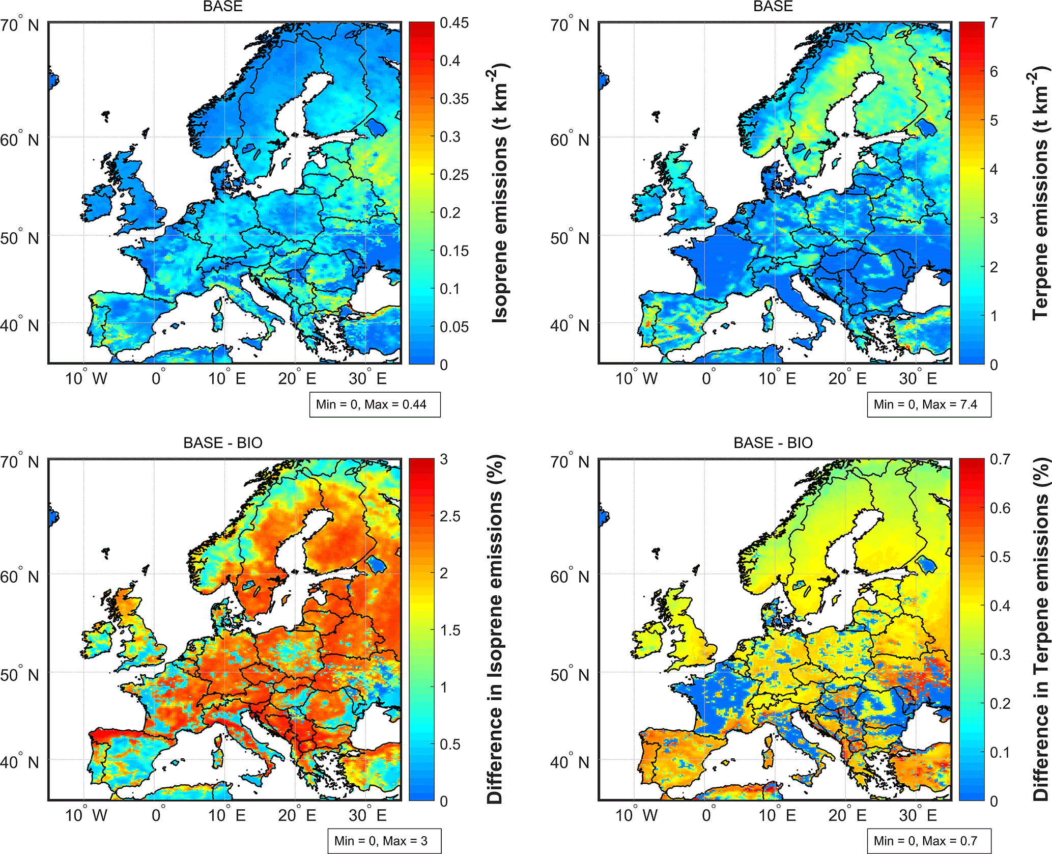
Figure 9Total (i.e., JJA sum) of isoprene (left panels) and terpene (monoterpene and sesquiterpene; right panels) emissions per km2 for the BASE scenario (top panels) and relative difference between BASE and BIO scenarios (bottom panels) in summer 2010.
The impact of a 2.5–3 and 0.7 % increase in isoprene and terpene emissions (BIO scenario), respectively, on daytime (10:00–18:00 LMT) average surface ozone is rather small (up to 0.08 ppb, ∼ 0.2 %; Fig. 10a) and an order of magnitude smaller than the respective ozone impact via photolysis rates (see Fig. 8). Both the daytime average and largest hourly (∼ 1 ppb) impacts are higher in central Europe where both BVOC and NOx emissions are ample (Figs. 10a and S7). The effects of increased BVOC emissions are higher in magnitude (up to 0.11 ppb, ∼ 0.3 %) and spatial coverage when applied to the base case with higher NOx emissions (i.e., BASE_NOx–BIO_NOx), as shown in Figs. 10b and S7. The combined effects via BVOC emissions and photolysis rates (COMBO and COMBO_NOx scenarios) on surface ozone appear to be roughly additive, with the photolysis rates effects dominating the overall impact (daytime average difference was up to 0.8 ppb, 1.5 %; Figs. 10c–d and S7). Overall, the direct effects of SSR changes on the BVOC emissions (with the assumptions and parameterizations of this study) were small, and as a result this was also the case for the consequent impact on surface ozone. However, SSR trend implications related to temperature and CO2 changes (Wild et al., 2007; Storelvmo et al., 2016) might have a more significant impact on BVOC emissions and thus on surface ozone, but this was beyond the scope of this study.
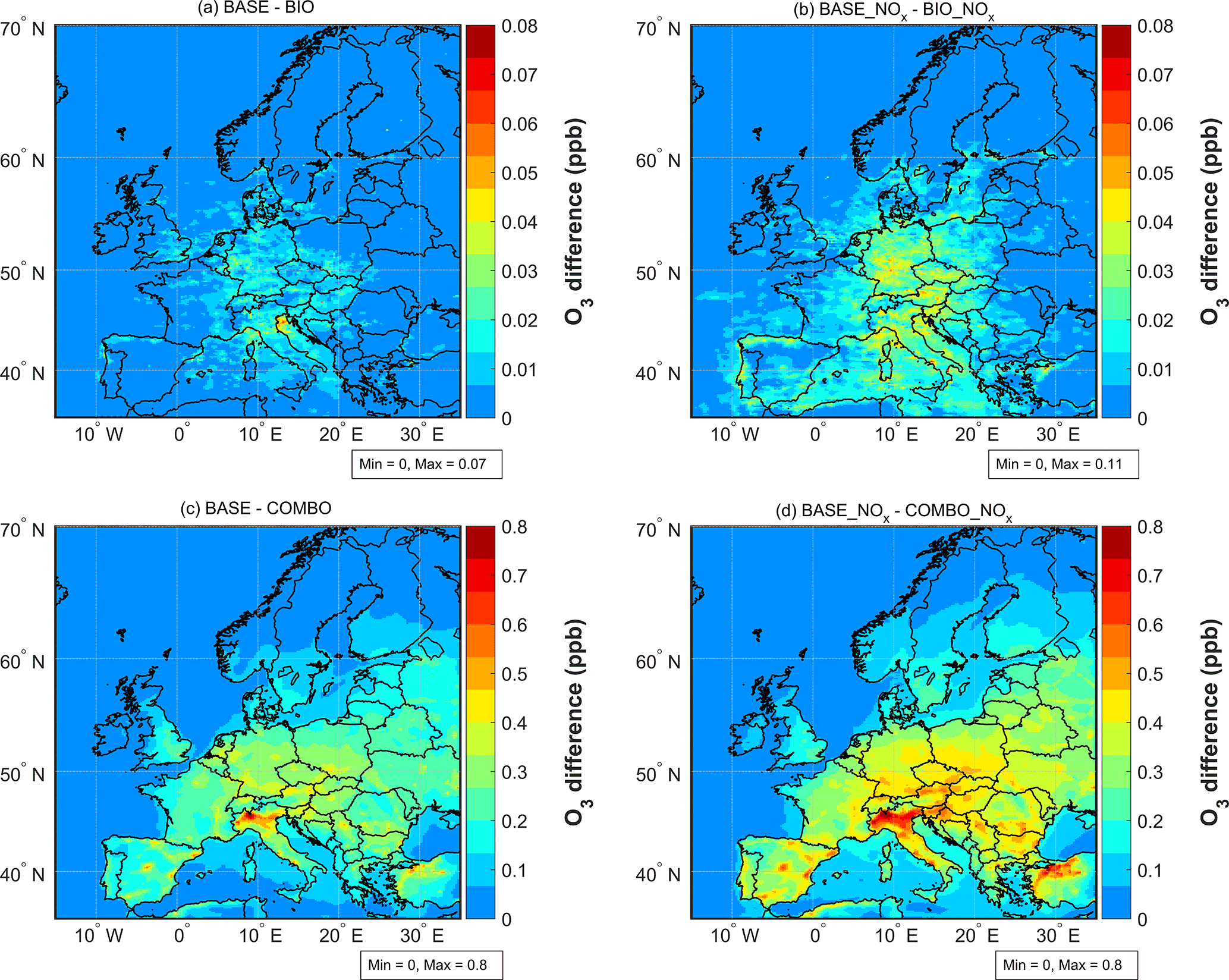
Figure 10Seasonal daytime (10:00–18:00 LMT) mean O3 differences between the (a) BASE and BIO, (b) BASE_NOx and BIO_NOx, (c) BASE and COMBO, and (d) BASE_NOx and COMBO_NOx scenarios in summer 2010.
4.6 ARI and ozone trends
Although the effects of ARI changes via photolysis rates and BVOC emissions on surface ozone seem to be small compared to the total ozone concentrations, it might be more meaningful to compare with the magnitude of the observed ozone concentration trends. Wilson et al. (2012) reported an annual (summer) increasing trend of 0.16 ± 0.02 (0.12 ± 0.06) ppb yr−1 in the European ground-level ozone (stations' average) for the period 1996–2005. The total ozone difference (0.2–0.8 ppb) via both the effects on photolysis rates and BVOC emissions (COMBO scenario) would translate (considering the full 20-year time period) to a summer trend of 0.01–0.04 ppb yr−1. These values should not be considered for a direct comparison with the absolute values of the aforementioned observed ozone trends, not only due to differences in the data analysis like time averaging and spatial coverage but most importantly due to the exclusion of other physical and chemical processes influencing the ozone trends. Nevertheless, the comparison of the order of magnitude between the aforementioned values and the reported ozone trends suggests a higher importance of the impact of ARI (only via photolysis rates and BVOC emissions) on surface ozone than when just comparing to the total ozone concentrations. Therefore, this comparison indicates that the ARI (as investigated in this study) might have had an accountable impact on the European surface ozone trends since the 1990s and could have partially dampened the effects of ozone precursor emissions' reduction along with other more influential physical processes like intercontinental transport and stratosphere–troposphere exchange (Ordóñez et al., 2007; Derwent et al., 2008, 2015).
We investigated the impact of the ARI changes on European summer surface ozone between 1990 and 2010 using the CAMx air quality model. We modeled the summer of 2010 as base case and designed various sensitivity tests based on literature review as well as an observational PM trend analysis performed in this study to represent the AOD and SSR conditions of the year 1990. One of the main assumptions in this study was that the change in ARI was the main driver for the solar brightening in Europe and thus excluded the ACI and cloud cover natural variability. Moreover, this study focused on the less uncertain effects of ARI via the impact on photolysis rates and BVOC emissions, compared to the more uncertain ARI-induced meteorological effects. Lastly, in the model scenarios, we assumed that the AOD changes between 1990 and 2010 in Europe were predominantly driven by changes in the anthropogenic PM2.5 concentrations, and hence we excluded any AOD changes due to variations in PM10 or natural PM2.5 concentrations.
Regarding the impact on ozone via photolysis rates, the PHOT1 and PHOT3 model scenarios (doubling anthropogenic PM2.5 concentrations and increasing only sulfate concentrations by 3.4 times, respectively) were considered to be closer to the observed and modeled AOD and SSR changes reported by other studies (see Sect. 4.3.1 and 4.3.2) compared to PHOT2 scenario (tripling anthropogenic PM2.5 concentrations) that should be regarded as an upper limit. Furthermore, the PHOT3 scenario was based on less uncertain assumptions (well-documented sulfate concentration trends; see Sects. 2.3.1 and 3), and therefore we considered it to be more realistic (except for southeastern Europe where the effects might be overestimated). The differences in AOD, SSR and the main ground-level photolysis rates (J(NO2) and J(O3 → O1D)) between the BASE and PHOT3 scenarios (representing the changes between summer of 1990 and 2010) were −0.33, 11 W m−2 and 4 %, respectively, and the consequent impact on daytime (10:00–18:00 LMT) surface ozone was on average 0.2–0.4 ppb (0.5–1 %) over central and western Europe. Moreover, the largest hourly difference in surface ozone could be as high as 4 ppb (10 %), while the same test performed on a base case with higher NOx emissions and ozone production (BASE_NOx–PHOT3_NOx) resulted in an extension of the spatial coverage of the ARI effects on ozone (apart from the VOC-limited Benelux region).
On the other hand, the impact of −3 % SSR change resulted in a near-linear response in isoprene emissions (2.5–3 %) but less in the terpene (monoterpene and sesquiterpene) emissions (0.7 %), with the subsequent effects on daytime ozone being small (up to 0.08 ppb, ∼ 0.2 %). Compared to the impact on ozone via the photolysis rates, the effects of BVOC emission changes were about an order of magnitude smaller, and thus the former dominated the latter impact when they were combined, as their effects were nearly additive. Therefore, the overall impact of SSR changes on ozone remained relatively small. Nevertheless, the role of the ARI changes (as quantified in this study) in the European summer surface ozone trends was suggested to be more important when comparing to the order of magnitude of the ozone trends instead of the total ozone concentrations.
Finally, the inclusion of the impact of ARI on meteorology and ACI might have additional increasing or, conversely, decreasing effects on surface ozone as discussed in Sect. 1. However, climate modeling studies show that the decline of aerosols can also affect the global atmospheric circulation as well as the atmospheric stability (Rotstayn et al., 2014; Wang et al., 2016; Navarro et al., 2017) and this entanglement might have compelling implications for air quality at a regional scale. It is therefore suggested that future air quality studies take into account the possible repercussions of declining aerosols on climate and atmospheric circulation at a global scale for a better understanding of the anthropogenic influence on air quality and climate as well as their complex interlinkage.
All data are available upon request from the corresponding authors.
The supplement related to this article is available online at: https://doi.org/10.5194/acp-18-9741-2018-supplement.
EO carried out the model simulations and data analysis. GC contributed to the model setup. SA, AP and UB planned and supervised the project and provided critical suggestions. MW co-supervised the analysis and provided reconstructive feedback. EO drafted the manuscript. All authors discussed and contributed to the writing of the final manuscript.
The authors declare that they have no conflict of interest.
We would like to thank the following agencies for preparing the datasets
used in this study: TNO for the anthropogenic emission inventory; the
European Environmental Agency (EEA) and the Swiss National Air Pollution
Monitoring Network (NABEL) for the air quality data; the European Centre for
Medium-Range Weather Forecasts (ECMWF) and Baseline Surface Radiation
Network (BSRN) for the meteorological data; the National Aeronautics and
Space Administration (NASA) and its data-contributing agencies (NCAR, UCAR,
AERONET) for the TOMS, MODIS and AOD data, the global air quality model data
and the TUV model. Calculations of meteorological data were performed with
the Swiss National Supercomputing Centre (CSCS). Our thanks extend to
RAMBOLL and especially Cristopher Emery for their continuous support
of the CAMx model. Finally, we would like to thank the two anonymous
referees for their constructive comments that helped to improve our
manuscript. This work was financially supported by the Swiss Federal Office
of Environment (FOEN).
Edited by: Jason West
Reviewed by: two anonymous referees
Aksoyoglu, S., Keller, J., Ciarelli, G., Prévôt, A. S. H., and Baltensperger, U.: A model study on changes of European and Swiss particulate matter, ozone and nitrogen deposition between 1990 and 2020 due to the revised Gothenburg protocol, Atmos. Chem. Phys., 14, 13081–13095, https://doi.org/10.5194/acp-14-13081-2014, 2014.
Aksoyoglu, S., Baltensperger, U., and Prévôt, A. S. H.: Contribution of ship emissions to the concentration and deposition of air pollutants in Europe, Atmos. Chem. Phys., 16, 1895–1906, https://doi.org/10.5194/acp-16-1895-2016, 2016.
Allen, R. J., Norris, J. R., and Wild, M.: Evaluation of multidecadal variability in CMIP5 surface solar radiation and inferred underestimation of aerosol direct effects over Europe, China, Japan, and India, J. Geophys. Res., 118, 6311–6336, https://doi.org/10.1002/jgrd.50426, 2013.
Andreani-Aksoyoglu, S. and Keller, J.: Estimates of monoterpene and isoprene emissions from the forests in Switzerland, J. Atmos. Chem., 20, 71–87, https://doi.org/10.1007/BF01099919, 1995.
Andreani-Aksoyoglu, S., Keller, J., Ordóñez, C., Tinguely, M., Schultz, M., and Prévôt, A. S. H.: Influence of various emission scenarios on ozone in Europe, Ecol. Model., 217, 209–218, https://doi.org/10.1016/j.ecolmodel.2008.06.022, 2008.
Augustine, J. A. and Dutton, E. G.: Variability of the surface radiation budget over the United States from 1996 through 2011 from high-quality measurements, J. Geophys. Res., 118, 43–53, https://doi.org/10.1029/2012JD018551, 2013.
Baklanov, A., Schlünzen, K., Suppan, P., Baldasano, J., Brunner, D., Aksoyoglu, S., Carmichael, G., Douros, J., Flemming, J., Forkel, R., Galmarini, S., Gauss, M., Grell, G., Hirtl, M., Joffre, S., Jorba, O., Kaas, E., Kaasik, M., Kallos, G., Kong, X., Korsholm, U., Kurganskiy, A., Kushta, J., Lohmann, U., Mahura, A., Manders-Groot, A., Maurizi, A., Moussiopoulos, N., Rao, S. T., Savage, N., Seigneur, C., Sokhi, R. S., Solazzo, E., Solomos, S., Sørensen, B., Tsegas, G., Vignati, E., Vogel, B., and Zhang, Y.: Online coupled regional meteorology chemistry models in Europe: current status and prospects, Atmos. Chem. Phys., 14, 317–398, https://doi.org/10.5194/acp-14-317-2014, 2014.
Banzhaf, S., Schaap, M., Kranenburg, R., Manders, A. M. M., Segers, A. J., Visschedijk, A. J. H., Denier van der Gon, H. A. C., Kuenen, J. J. P., van Meijgaard, E., van Ulft, L. H., Cofala, J., and Builtjes, P. J. H.: Dynamic model evaluation for secondary inorganic aerosol and its precursors over Europe between 1990 and 2009, Geosci. Model Dev., 8, 1047–1070, https://doi.org/10.5194/gmd-8-1047-2015, 2015.
Barmpadimos, I., Hueglin, C., Keller, J., Henne, S., and Prévôt, A. S. H.: Influence of meteorology on PM10 trends and variability in Switzerland from 1991 to 2008, Atmos. Chem. Phys., 11, 1813–1835, https://doi.org/10.5194/acp-11-1813-2011, 2011.
Barmpadimos, I., Keller, J., Oderbolz, D., Hueglin, C., and Prévôt, A. S. H.: One decade of parallel fine (PM2.5) and coarse (PM10–PM2.5) particulate matter measurements in Europe: trends and variability, Atmos. Chem. Phys., 12, 3189–3203, https://doi.org/10.5194/acp-12-3189-2012, 2012.
Bessagnet, B., Pirovano, G., Mircea, M., Cuvelier, C., Aulinger, A., Calori, G., Ciarelli, G., Manders, A., Stern, R., Tsyro, S., García Vivanco, M., Thunis, P., Pay, M.-T., Colette, A., Couvidat, F., Meleux, F., Rouïl, L., Ung, A., Aksoyoglu, S., Baldasano, J. M., Bieser, J., Briganti, G., Cappelletti, A., D'Isidoro, M., Finardi, S., Kranenburg, R., Silibello, C., Carnevale, C., Aas, W., Dupont, J.-C., Fagerli, H., Gonzalez, L., Menut, L., Prévôt, A. S. H., Roberts, P., and White, L.: Presentation of the EURODELTA III intercomparison exercise – evaluation of the chemistry transport models' performance on criteria pollutants and joint analysis with meteorology, Atmos. Chem. Phys., 16, 12667–12701, https://doi.org/10.5194/acp-16-12667-2016, 2016.
Bian, H. and Prather, M. J.: Fast-J2: Accurate Simulation of Stratospheric Photolysis in Global Chemical Models, J. Atmos. Chem., 41, 281–296, https://doi.org/10.1023/a:1014980619462, 2002.
Bian, H., Prather, M. J., and Takemura, T.: Tropospheric aerosol impacts on trace gas budgets through photolysis, J. Geophys. Res., 108, 4242, https://doi.org/10.1029/2002JD002743, 2003.
Bin, Z., Jonathan, H. J., Yu, G., David, D., John, W., Kuo-Nan, L., Hui, S., Jia, X., Michael, G., and Lei, H.: Decadal-scale trends in regional aerosol particle properties and their linkage to emission changes, Environ. Res. Lett., 12, 054021, https://doi.org/10.1088/1748-9326/aa6cb2, 2017.
Boers, R., Brandsma, T., and Siebesma, A. P.: Impact of aerosols and clouds on decadal trends in all-sky solar radiation over the Netherlands (1966–2015), Atmos. Chem. Phys., 17, 8081–8100, https://doi.org/10.5194/acp-17-8081-2017, 2017.
Cermak, J., Wild, M., Knutti, R., Mishchenko, M. I., and Heidinger, A. K.: Consistency of global satellite-derived aerosol and cloud data sets with recent brightening observations, Geophys. Res. Lett., 37, L21704, https://doi.org/10.1029/2010GL044632, 2010.
Cesnulyte, V., Lindfors, A. V., Pitkänen, M. R. A., Lehtinen, K. E. J., Morcrette, J.-J., and Arola, A.: Comparing ECMWF AOD with AERONET observations at visible and UV wavelengths, Atmos. Chem. Phys., 14, 593–608, https://doi.org/10.5194/acp-14-593-2014, 2014.
Cherian, R., Quaas, J., Salzmann, M., and Wild, M.: Pollution trends over Europe constrain global aerosol forcing as simulated by climate models, Geophys. Res. Lett., 41, 2176–2181, https://doi.org/10.1002/2013GL058715, 2014.
Chiacchio, M. and Wild, M.: Influence of NAO and clouds on long-term seasonal variations of surface solar radiation in Europe, J. Geophys. Res., 115, D00D22, https://doi.org/10.1029/2009JD012182, 2010.
Chiacchio, M., Ewen, T., Wild, M., Chin, M., and Diehl, T.: Decadal variability of aerosol optical depth in Europe and its relationship to the temporal shift of the North Atlantic Oscillation in the realm of dimming and brightening, J. Geophys. Res., 116, D02108, https://doi.org/10.1029/2010JD014471, 2011.
Colette, A., Aas, W., Banin, L., Braban, C. F., Ferm, M., González Ortiz, A., Ilyin, I., Mar, K., Pandolfi, M., Putaud, J.-P., Shatalov, V., Solberg, S., Spindler, G., Tarasova, O., Vana, M., Adani, M., Almodovar, P., Berton, E., Bessagnet, B., Bohlin-Nizzetto, P., J., B., Breivik, K., Briganti, G., Cappelletti, A., Cuvelier, K., Derwent, R., D'Isidoro, M., Fagerli, H., Funk, C., Garcia Vivanco, M., Haeuber, R., Hueglin, C., Jenkins, S., Kerr, J., de Leeuw, F., Lynch, J., Manders, A., Mircea, M., Pay, M. T., Pritula, D., Querol, X., Raffort, V., Reiss, I., Roustan, Y., Sauvage, S., Scavo, K., Simpson, D., Smith, R. I., Tang, Y. S., Theobald, M., Tørseth, K., Tsyro, S., van Pul, A., Vidic, S., Wallasch, M., and Wind, P.: Air pollution trends in the EMEP region between 1990 and 2012, Joint report of: EMEP Task Force on Measurements and Modelling (TFMM), Chemical Co-ordinating Centre (CCC), Meteorological Synthesizing Centre-East (MSC-E), Meteorological Synthesizing Centre-West (MSC-W), Norwegian Institute for Air Research, https://www.unece.org/index.php?id=42906 (last access: 2 July 2018), 2016.
Colette, A., Andersson, C., Manders, A., Mar, K., Mircea, M., Pay, M.-T., Raffort, V., Tsyro, S., Cuvelier, C., Adani, M., Bessagnet, B., Bergström, R., Briganti, G., Butler, T., Cappelletti, A., Couvidat, F., D'Isidoro, M., Doumbia, T., Fagerli, H., Granier, C., Heyes, C., Klimont, Z., Ojha, N., Otero, N., Schaap, M., Sindelarova, K., Stegehuis, A. I., Roustan, Y., Vautard, R., van Meijgaard, E., Vivanco, M. G., and Wind, P.: EURODELTA-Trends, a multi-model experiment of air quality hindcast in Europe over 1990–2010, Geosci. Model Dev., 10, 3255–3276, https://doi.org/10.5194/gmd-10-3255-2017, 2017.
Curci, G., Hogrefe, C., Bianconi, R., Im, U., Balzarini, A., Baró, R., Brunner, D., Forkel, R., Giordano, L., Hirtl, M., Honzak, L., Jiménez-Guerrero, P., Knote, C., Langer, M., Makar, P. A., Pirovano, G., Pérez, J. L., San José, R., Syrakov, D., Tuccella, P., Werhahn, J., Wolke, R., Žabkar, R., Zhang, J., and Galmarini, S.: Uncertainties of simulated aerosol optical properties induced by assumptions on aerosol physical and chemical properties: An AQMEII-2 perspective, Atmos. Environ., 115, 541–552, https://doi.org/10.1016/j.atmosenv.2014.09.009, 2015.
Derwent, R. G., Stevenson, D. S., Doherty, R. M., Collins, W. J., and Sanderson, M. G.: How is surface ozone in Europe linked to Asian and North American NOx emissions?, Atmos. Environ., 42, 7412–7422, https://doi.org/10.1016/j.atmosenv.2008.06.037, 2008.
Derwent, R. G., Utembe, S. R., Jenkin, M. E., and Shallcross, D. E.: Tropospheric ozone production regions and the intercontinental origins of surface ozone over Europe, Atmos. Environ., 112, 216–224, https://doi.org/10.1016/j.atmosenv.2015.04.049, 2015.
Dutton, E. G., Nelson, D. W., Stone, R. S., Longenecker, D., Carbaugh, G., Harris, J. M., and Wendell, J.: Decadal variations in surface solar irradiance as observed in a globally remote network, J. Geophys. Res., 111, D19101, https://doi.org/10.1029/2005JD006901, 2006.
Eck, T. F., Holben, B. N., Reid, J. S., Dubovik, O., Smirnov, A., O'Neill, N. T., Slutsker, I., and Kinne, S.: Wavelength dependence of the optical depth of biomass burning, urban, and desert dust aerosols, J. Geophys. Res., 104, 31333–31349, https://doi.org/10.1029/1999JD900923, 1999.
EEA: Emissions of primary PM2.5 and PM10 particulate matter, European Environment Agency, Copenhagen, 2014.
EEA: Emissions of the main air pollutants in Europe, European Environment Agency, Copenhagen, 2017.
Elterman, L.: UV, Visible, and IR Attenuation for Altitudes to 50 km, Technical Report AFCRL-68-0153, Air Force Geophysics Laboratory, Hanscom Air Force Base, Bedford, MA, USA, 1968.
Emery, C., Jung, J., Johnson, J., Yarwood, G., Madronich, S., and Grell, G.: Improving the Characterization of Clouds and their Impact on Photolysis Rates within the CAMx Photochemical Grid Model, Prepared for the Texas Commission on Environmental Quality, Austin, TX, Prepared by ENVIRON International Corporation, Novato, CA and the National Center for Atmospheric Research, Boulder, CO (27 August 2010), 2010.
Empa: Technischer Bericht zum Nationalen Beobachtungsnetz für Luftfremdstoffe (NABEL), Empa, Duebendorf, Switzerland, https://doi.org/10.3929/ethz-a-006173107, 2010.
Eyring, V., Köhler, H. W., van Aardenne, J., and Lauer, A.: Emissions from international shipping: 1. The last 50 years, J. Geophys. Res., 110, D17305, 10.1029/2004JD005619, 2005.
FLAG: Federal Land Managers' Air Quality Related Values Workgroup (FLAG), Phase I Report, Prepared by the US Forest Service, Air Quality Program; National Park Service, Air Resources Division; and US Fish and Wildlife Service, Air Quality Branch (December 2000), Lakewood, Colorado, USA, 2000.
Folini, D. and Wild, M.: Aerosol emissions and dimming/brightening in Europe: Sensitivity studies with ECHAM5-HAM, J. Geophys. Res., 116, D21104, https://doi.org/10.1029/2011JD016227, 2011.
Forkel, R., Werhahn, J., Hansen, A. B., McKeen, S., Peckham, S., Grell, G., and Suppan, P.: Effect of aerosol-radiation feedback on regional air quality – A case study with WRF/Chem, Atmos. Environ., 53, 202–211, https://doi.org/10.1016/j.atmosenv.2011.10.009, 2012.
Forkel, R., Balzarini, A., Baró, R., Bianconi, R., Curci, G., Jiménez-Guerrero, P., Hirtl, M., Honzak, L., Lorenz, C., Im, U., Pérez, J. L., Pirovano, G., San José, R., Tuccella, P., Werhahn, J., and Žabkar, R.: Analysis of the WRF-Chem contributions to AQMEII phase2 with respect to aerosol radiative feedbacks on meteorology and pollutant distributions, Atmos. Environ., 115, 630–645, https://doi.org/10.1016/j.atmosenv.2014.10.056, 2015.
Fuzzi, S., Baltensperger, U., Carslaw, K., Decesari, S., Denier van der Gon, H., Facchini, M. C., Fowler, D., Koren, I., Langford, B., Lohmann, U., Nemitz, E., Pandis, S., Riipinen, I., Rudich, Y., Schaap, M., Slowik, J. G., Spracklen, D. V., Vignati, E., Wild, M., Williams, M., and Gilardoni, S.: Particulate matter, air quality and climate: lessons learned and future needs, Atmos. Chem. Phys., 15, 8217–8299, https://doi.org/10.5194/acp-15-8217-2015, 2015.
Genio, A. D. D., Yao, M.-S., Kovari, W., and Lo, K. K.-W.: A prognostic cloud water parameterization for global climate models, J. Climate, 9, 270–304, https://doi.org/10.1175/1520-0442(1996)009<0270:apcwpf>2.0.co;2, 1996.
Guenther, A.: Biological and chemical diversity of biogenic volatile organic emissions into the atmosphere, ISRN Atmospheric Sciences, 2013, 786290, https://doi.org/10.1155/2013/786290, 2013.
Guenther, A., Karl, T., Harley, P., Wiedinmyer, C., Palmer, P. I., and Geron, C.: Estimates of global terrestrial isoprene emissions using MEGAN (Model of Emissions of Gases and Aerosols from Nature), Atmos. Chem. Phys., 6, 3181–3210, https://doi.org/10.5194/acp-6-3181-2006, 2006.
Gustafson, E. J., Miranda, B. R., De Bruijn, A. M. G., Sturtevant, B. R., and Kubiske, M. E.: Do rising temperatures always increase forest productivity? Interacting effects of temperature, precipitation, cloudiness and soil texture on tree species growth and competition, Environ. Modell. Softw., 97, 171–183, https://doi.org/10.1016/j.envsoft.2017.08.001, 2017.
Hildebrandt Ruiz, L. H. and Yarwood, G.: Interactions between Organic Aerosol and NOy: Influence on Oxidant Production, Final Report for AQRP project 12–012, available at: http://aqrp.ceer.utexas.edu/projectinfoFY12_13/12-012/12-012 Final Report.pdf (last access: 2 July 2018), 2013.
Hogrefe, C., Pouliot, G., Wong, D., Torian, A., Roselle, S., Pleim, J., and Mathur, R.: Annual application and evaluation of the online coupled WRF-CMAQ system over North America under AQMEII phase 2, Atmos. Environ., 115, 683–694, https://doi.org/10.1016/j.atmosenv.2014.12.034, 2015.
Holben, B. N., Eck, T. F., Slutsker, I., Tanré, D., Buis, J. P., Setzer, A., Vermote, E., Reagan, J. A., Kaufman, Y. J., Nakajima, T., Lavenu, F., Jankowiak, I., and Smirnov, A.: AERONET – A Federated Instrument Network and Data Archive for Aerosol Characterization, Remote Sens. Environ., 66, 1–16, https://doi.org/10.1016/S0034-4257(98)00031-5, 1998.
Horowitz, L. W., Walters, S., Mauzerall, D. L., Emmons, L. K., Rasch, P. J., Granier, C., Tie, X., Lamarque, J. F., Schultz, M. G., and Tyndall, G. S.: A global simulation of tropospheric ozone and related tracers: Description and evaluation of MOZART, version 2, J. Geophys. Res., 108, 4784, https://doi.org/10.1029/2002JD002853, 2003.
Im, U., Bianconi, R., Solazzo, E., Kioutsioukis, I., Badia, A., Balzarini, A., Baró, R., Bellasio, R., Brunner, D., Chemel, C., Curci, G., Denier van der Gon, H., Flemming, J., Forkel, R., Giordano, L., Jiménez-Guerrero, P., Hirtl, M., Hodzic, A., Honzak, L., Jorba, O., Knote, C., Makar, P. A., Manders-Groot, A., Neal, L., Pérez, J. L., Pirovano, G., Pouliot, G., San Jose, R., Savage, N., Schroder, W., Sokhi, R. S., Syrakov, D., Torian, A., Tuccella, P., Wang, K., Werhahn, J., Wolke, R., Zabkar, R., Zhang, Y., Zhang, J., Hogrefe, C., and Galmarini, S.: Evaluation of operational online-coupled regional air quality models over Europe and North America in the context of AQMEII phase 2, Part II: Particulate matter, Atmos. Environ., 115, 421–441, https://doi.org/10.1016/j.atmosenv.2014.08.072, 2015.
Imamovic, A., Tanaka, K., Folini, D., and Wild, M.: Global dimming and urbanization: did stronger negative SSR trends collocate with regions of population growth?, Atmos. Chem. Phys., 16, 2719–2725, https://doi.org/10.5194/acp-16-2719-2016, 2016.
Karamchandani, P., Long, Y., Pirovano, G., Balzarini, A., and Yarwood, G.: Source-sector contributions to European ozone and fine PM in 2010 using AQMEII modeling data, Atmos. Chem. Phys., 17, 5643–5664, https://doi.org/10.5194/acp-17-5643-2017, 2017.
Karl, M., Guenther, A., Köble, R., Leip, A., and Seufert, G.: A new European plant-specific emission inventory of biogenic volatile organic compounds for use in atmospheric transport models, Biogeosciences, 6, 1059–1087, https://doi.org/10.5194/bg-6-1059-2009, 2009.
Kendall, M. G.: Rank correlation methods, Griffin, Oxford, England, 1948.
Kong, X., Forkel, R., Sokhi, R. S., Suppan, P., Baklanov, A., Gauss, M., Brunner, D., Barò, R., Balzarini, A., Chemel, C., Curci, G., Jiménez-Guerrero, P., Hirtl, M., Honzak, L., Im, U., Pérez, J. L., Pirovano, G., San Jose, R., Schlünzen, K. H., Tsegas, G., Tuccella, P., Werhahn, J., Žabkar, R., and Galmarini, S.: Analysis of meteorology-chemistry interactions during air pollution episodes using online coupled models within AQMEII phase-2, Atmos. Environ., 115, 527–540, https://doi.org/10.1016/j.atmosenv.2014.09.020, 2015.
König-Langlo, G., Sieger, R., Schmithüsen, H., Bücker, A., Richter, F., and Dutton, E.: The baseline surface radiation network and its world radiation monitoring centre at the Alfred Wegener Institute, GCOS – 174, WCRP Report 24/2013, World Meteorological Organization (WMO), Geneva, Switzerland, 30 pp., https://doi.org/10013/epic.42596.d001, 2013.
Kuenen, J. J. P., Visschedijk, A. J. H., Jozwicka, M., and Denier van der Gon, H. A. C.: TNO-MACC_II emission inventory; a multi-year (2003–2009) consistent high-resolution European emission inventory for air quality modelling, Atmos. Chem. Phys., 14, 10963–10976, https://doi.org/10.5194/acp-14-10963-2014, 2014.
Kuik, F., Lauer, A., Churkina, G., Denier van der Gon, H. A. C., Fenner, D., Mar, K. A., and Butler, T. M.: Air quality modelling in the Berlin-Brandenburg region using WRF-Chem v3.7.1: sensitivity to resolution of model grid and input data, Geosci. Model Dev., 9, 4339–4363, https://doi.org/10.5194/gmd-9-4339-2016, 2016.
Kushta, J., Kallos, G., Astitha, M., Solomos, S., Spyrou, C., Mitsakou, C., and Lelieveld, J.: Impact of natural aerosols on atmospheric radiation and consequent feedbacks with the meteorological and photochemical state of the atmosphere, J. Geophys. Res., 119, 1463–1491, https://doi.org/10.1002/2013JD020714, 2014.
Kvalevåg, M. M. and Myhre, G.: Human Impact on Direct and Diffuse Solar Radiation during the Industrial Era, J. Climate, 20, 4874–4883, https://doi.org/10.1175/jcli4277.1, 2007.
Lathière, J., Hauglustaine, D. A., Friend, A. D., De Noblet-Ducoudré, N., Viovy, N., and Folberth, G. A.: Impact of climate variability and land use changes on global biogenic volatile organic compound emissions, Atmos. Chem. Phys., 6, 2129–2146, https://doi.org/10.5194/acp-6-2129-2006, 2006.
Li, J., Carlson, B. E., and Lacis, A. A.: Revisiting AVHRR tropospheric aerosol trends using principal component analysis, J. Geophys. Res., 119, 3309–3320, https://doi.org/10.1002/2013JD020789, 2014a.
Li, J., Carlson, B. E., Dubovik, O., and Lacis, A. A.: Recent trends in aerosol optical properties derived from AERONET measurements, Atmos. Chem. Phys., 14, 12271–12289, https://doi.org/10.5194/acp-14-12271-2014, 2014b.
Lohmann, U. and Feichter, J.: Global indirect aerosol effects: a review, Atmos. Chem. Phys., 5, 715–737, https://doi.org/10.5194/acp-5-715-2005, 2005.
Long, C. N., Dutton, E. G., Augustine, J. A., Wiscombe, W., Wild, M., McFarlane, S. A., and Flynn, C. J.: Significant decadal brightening of downwelling shortwave in the continental United States, J. Geophys. Res., 114, D00D06, https://doi.org/10.1029/2008JD011263, 2009.
Madronich, S. and Flocke, S.: The Role of Solar Radiation in Atmospheric Chemistry, in: Environmental Photochemistry, edited by: Boule, P., Springer Berlin Heidelberg, Berlin, Heidelberg, 1–26, 1999.
Mailler, S., Menut, L., di Sarra, A. G., Becagli, S., Di Iorio, T., Bessagnet, B., Briant, R., Formenti, P., Doussin, J.-F., Gómez-Amo, J. L., Mallet, M., Rea, G., Siour, G., Sferlazzo, D. M., Traversi, R., Udisti, R., and Turquety, S.: On the radiative impact of aerosols on photolysis rates: comparison of simulations and observations in the Lampedusa island during the ChArMEx/ADRIMED campaign, Atmos. Chem. Phys., 16, 1219–1244, https://doi.org/10.5194/acp-16-1219-2016, 2016.
Makar, P. A., Gong, W., Hogrefe, C., Zhang, Y., Curci, G., Žabkar, R., Milbrandt, J., Im, U., Balzarini, A., Baró, R., Bianconi, R., Cheung, P., Forkel, R., Gravel, S., Hirtl, M., Honzak, L., Hou, A., Jiménez-Guerrero, P., Langer, M., Moran, M. D., Pabla, B., Pérez, J. L., Pirovano, G., San José, R., Tuccella, P., Werhahn, J., Zhang, J., and Galmarini, S.: Feedbacks between air pollution and weather, part 2: Effects on chemistry, Atmos. Environ., 115, 499–526, https://doi.org/10.1016/j.atmosenv.2014.10.021, 2015a.
Makar, P. A., Gong, W., Milbrandt, J., Hogrefe, C., Zhang, Y., Curci, G., Žabkar, R., Im, U., Balzarini, A., Baró, R., Bianconi, R., Cheung, P., Forkel, R., Gravel, S., Hirtl, M., Honzak, L., Hou, A., Jiménez-Guerrero, P., Langer, M., Moran, M. D., Pabla, B., Pérez, J. L., Pirovano, G., San José, R., Tuccella, P., Werhahn, J., Zhang, J., and Galmarini, S.: Feedbacks between air pollution and weather, Part 1: Effects on weather, Atmos. Environ., 115, 442–469, https://doi.org/10.1016/j.atmosenv.2014.12.003, 2015b.
Manara, V., Brunetti, M., Celozzi, A., Maugeri, M., Sanchez-Lorenzo, A., and Wild, M.: Detection of dimming/brightening in Italy from homogenized all-sky and clear-sky surface solar radiation records and underlying causes (1959–2013), Atmos. Chem. Phys., 16, 11145–11161, https://doi.org/10.5194/acp-16-11145-2016, 2016.
Mann, H. B.: Nonparametric tests against trend, Econometrica, 13, 245–259, https://doi.org/10.2307/1907187, 1945.
Mei, L., Xue, Y., de Leeuw, G., Guang, J., Wang, Y., Li, Y., Xu, H., Yang, L., Hou, T., He, X., Wu, C., Dong, J., and Chen, Z.: Integration of remote sensing data and surface observations to estimate the impact of the Russian wildfires over Europe and Asia during August 2010, Biogeosciences, 8, 3771–3791, https://doi.org/10.5194/bg-8-3771-2011, 2011.
Mercado, L. M., Bellouin, N., Sitch, S., Boucher, O., Huntingford, C., Wild, M., and Cox, P. M.: Impact of changes in diffuse radiation on the global land carbon sink, Nature, 458, 1014, https://doi.org/10.1038/nature07949, 2009.
Messina, P., Lathière, J., Sindelarova, K., Vuichard, N., Granier, C., Ghattas, J., Cozic, A., and Hauglustaine, D. A.: Global biogenic volatile organic compound emissions in the ORCHIDEE and MEGAN models and sensitivity to key parameters, Atmos. Chem. Phys., 16, 14169–14202, https://doi.org/10.5194/acp-16-14169-2016, 2016.
Mishchenko, M. I., Geogdzhayev, I. V., Rossow, W. B., Cairns, B., Carlson, B. E., Lacis, A. A., Liu, L., and Travis, L. D.: Long-term satellite record reveals likely recent aerosol trend, Science, 315, 1543–1543, https://doi.org/10.1126/science.1136709, 2007.
Mol, W., and de Leeuw, F.: AirBase: a valuable tool in air quality assessments, Proceedings of the 5th International Conference on Urban Air Quality, edited by: Sokhi, R. S, Millán, M. M, and Moussiopoulos, N., Valencia, Spain, 2005,
Monks, P. S.: Gas-phase radical chemistry in the troposphere, Chem. Soc. Rev., 34, 376–395, https://doi.org/10.1039/B307982C, 2005.
Nabat, P., Somot, S., Mallet, M., Sanchez-Lorenzo, A., and Wild, M.: Contribution of anthropogenic sulfate aerosols to the changing Euro-Mediterranean climate since 1980, Geophys. Res. Lett., 41, 5605–5611, https://doi.org/10.1002/2014GL060798, 2014.
Navarro, J. C. A., Ekman, A. M. L., Pausata, F. S. R., Lewinschal, A., Varma, V., Seland, Ø., Gauss, M., Iversen, T., Kirkevåg, A., Riipinen, I., and Hansson, H. C.: Future response of temperature and precipitation to reduced aerosol missions as compared with increased greenhouse gas concentrations, J. Climate, 30, 939–954, https://doi.org/10.1175/jcli-d-16-0466.1, 2017.
NCAR: The Tropospheric Visible and Ultraviolet (TUV) Radiation Model web page, National Center for Atmospheric Research, Atmospheric Chemistry Division, Boulder, Colorado, available at: https://www2.acom.ucar.edu/modeling/tropospheric-ultraviolet-and-visible-tuv-radiation-model (last access: 2 July 2018), 2011.
Nenes, A., Pandis, S. N., and Pilinis, C.: ISORROPIA: A new thermodynamic equilibrium model for multiphase multicomponent inorganic aerosols, Aquat. Geochem., 4, 123–152, https://doi.org/10.1023/A:1009604003981, 1998.
Nenes, A., Pandis, S. N., and Pilinis, C.: Continued development and testing of a new thermodynamic aerosol module for urban and regional air quality models, Atmos. Environ., 33, 1553–1560, https://doi.org/10.1016/S1352-2310(98)00352-5, 1999.
Norris, J. R. and Wild, M.: Trends in aerosol radiative effects over Europe inferred from observed cloud cover, solar “dimming,” and solar “brightening”, J. Geophys. Res., 112, D08214, https://doi.org/10.1029/2006JD007794, 2007.
Oderbolz, D. C., Aksoyoglu, S., Keller, J., Barmpadimos, I., Steinbrecher, R., Skjøth, C. A., Plaß-Dülmer, C., and Prévôt, A. S. H.: A comprehensive emission inventory of biogenic volatile organic compounds in Europe: improved seasonality and land-cover, Atmos. Chem. Phys., 13, 1689–1712, https://doi.org/10.5194/acp-13-1689-2013, 2013.
Ohmura, A.: Observed decadal variations in surface solar radiation and their causes, J. Geophys. Res., 114, https://doi.org/10.1029/2008JD011290, D00D05, 2009.
Oikonomakis, E., Aksoyoglu, S., Ciarelli, G., Baltensperger, U., and Prévôt, A. S. H.: Low modeled ozone production suggests underestimation of precursor emissions (especially NOx) in Europe, Atmos. Chem. Phys., 18, 2175–2198, https://doi.org/10.5194/acp-18-2175-2018, 2018
O'Neill, N. T., Eck, T. F., Smirnov, A., Holben, B. N., and Thulasiraman, S.: Spectral discrimination of coarse and fine mode optical depth, J. Geophys. Res., 108, 4559, https://doi.org/10.1029/2002JD002975, 2003.
Ordóñez, C., Mathis, H., Furger, M., Henne, S., Hüglin, C., Staehelin, J., and Prévôt, A. S. H.: Changes of daily surface ozone maxima in Switzerland in all seasons from 1992 to 2002 and discussion of summer 2003, Atmos. Chem. Phys., 5, 1187–1203, https://doi.org/10.5194/acp-5-1187-2005, 2005.
Ordóñez, C., Brunner, D., Staehelin, J., Hadjinicolaou, P., Pyle, J. A., Jonas, M., Wernli, H., and Prévôt, A. S. H.: Strong influence of lowermost stratospheric ozone on lower tropospheric background ozone changes over Europe, Geophys. Res. Lett., 34, L07805, https://doi.org/10.1029/2006GL029113, 2007.
Parding, K. M., Liepert, B. G., Hinkelman, L. M., Ackerman, T. P., Dagestad, K.-F., and Olseth, J. A.: Influence of Synoptic Weather Patterns on Solar Irradiance Variability in Northern Europe, J. Climate, 29, 4229–4250, https://doi.org/10.1175/jcli-d-15-0476.1, 2016.
Péré, J. C., Bessagnet, B., Pont, V., Mallet, M., and Minvielle, F.: Influence of the aerosol solar extinction on photochemistry during the 2010 Russian wildfires episode, Atmos. Chem. Phys., 15, 10983–10998, https://doi.org/10.5194/acp-15-10983-2015, 2015
Petropavlovskikh, I.: Evaluation of photodissociation coefficient calculations for use in atmospheric chemical models, PhD thesis, University of Brussels/National Center for Atmospheric Research, Cooperative Thesis No. 159, NCAR, Boulder, Colorado, USA, 1995.
Portin, H., Mielonen, T., Leskinen, A., Arola, A., Pärjälä, E., Romakkaniemi, S., Laaksonen, A., Lehtinen, K. E. J., and Komppula, M.: Biomass burning aerosols observed in Eastern Finland during the Russian wildfires in summer 2010 – Part 1: In-situ aerosol characterization, Atmos. Environ., 47, 269–278, https://doi.org/10.1016/j.atmosenv.2011.10.067, 2012.
Putaud, J. P., Van Dingenen, R., Alastuey, A., Bauer, H., Birmili, W., Cyrys, J., Flentje, H., Fuzzi, S., Gehrig, R., Hansson, H. C., Harrison, R. M., Herrmann, H., Hitzenberger, R., Hüglin, C., Jones, A. M., Kasper-Giebl, A., Kiss, G., Kousa, A., Kuhlbusch, T. A. J., Löschau, G., Maenhaut, W., Molnar, A., Moreno, T., Pekkanen, J., Perrino, C., Pitz, M., Puxbaum, H., Querol, X., Rodriguez, S., Salma, I., Schwarz, J., Smolik, J., Schneider, J., Spindler, G., ten Brink, H., Tursic, J., Viana, M., Wiedensohler, A., and Raes, F.: A European aerosol phenomenology – 3: Physical and chemical characteristics of particulate matter from 60 rural, urban, and kerbside sites across Europe, Atmos. Environ., 44, 1308–1320, https://doi.org/10.1016/j.atmosenv.2009.12.011, 2010.
Ramboll Environ: User's guide to the Comprehensive Air Quality Model with Extensions (CAMx), Version 6.3, available at: http://www.camx.com (last access: 2 July 2018), 2016.
Real, E. and Sartelet, K.: Modeling of photolysis rates over Europe: impact on chemical gaseous species and aerosols, Atmos. Chem. Phys., 11, 1711–1727, https://doi.org/10.5194/acp-11-1711-2011, 2011.
Rotstayn, L. D., Plymin, E. L., Collier, M. A., Boucher, O., Dufresne, J.-L., Luo, J.-J., Salzen, K. v., Jeffrey, S. J., Foujols, M.-A., Ming, Y., and Horowitz, L. W.: Declining aerosols in CMIP5 Projections: effects on atmospheric temperature structure and midlatitude jets, J. Climate, 27, 6960–6977, https://doi.org/10.1175/jcli-d-14-00258.1, 2014.
Ruckstuhl, C., Philipona, R., Behrens, K., Collaud Coen, M., Dürr, B., Heimo, A., Mätzler, C., Nyeki, S., Ohmura, A., Vuilleumier, L., Weller, M., Wehrli, C., and Zelenka, A.: Aerosol and cloud effects on solar brightening and the recent rapid warming, Geophys. Res. Lett., 35, https://doi.org/10.1029/2008GL034228, L12708, 2008.
Ruckstuhl, C., and Norris, J. R.: How do aerosol histories affect solar “dimming” and “brightening” over Europe?: IPCC-AR4 models versus observations, J. Geophys. Res., 114, D00D04, https://doi.org/10.1029/2008JD011066, 2009.
Ruckstuhl, C., Norris, J. R., and Philipona, R.: Is there evidence for an aerosol indirect effect during the recent aerosol optical depth decline in Europe?, J. Geophys. Res., 115, D04204, https://doi.org/10.1029/2009JD012867, 2010.
Sanchez-Lorenzo, A. and Wild, M.: Decadal variations in estimated surface solar radiation over Switzerland since the late 19th century, Atmos. Chem. Phys., 12, 8635–8644, https://doi.org/10.5194/acp-12-8635-2012, 2012
Sanchez-Lorenzo, A., Calbó, J., and Martin-Vide, J.: Spatial and temporal trends in sunshine duration over western Europe (1938–2004), J. Climate, 21, 6089–6098, https://doi.org/10.1175/2008jcli2442.1, 2008.
Sanchez-Lorenzo, A., Calbó, J., Brunetti, M., and Deser, C.: Dimming/brightening over the Iberian Peninsula: Trends in sunshine duration and cloud cover and their relations with atmospheric circulation, J. Geophys. Res., 114, D00D09, https://doi.org/10.1029/2008JD011394, 2009.
Sanchez-Lorenzo, A., Calbó, J., and Wild, M.: Increasing cloud cover in the 20th century: review and new findings in Spain, Clim. Past, 8, 1199–1212, https://doi.org/10.5194/cp-8-1199-2012, 2012.
Sanchez-Lorenzo, A., Wild, M., Brunetti, M., Guijarro, J. A., Hakuba, M. Z., Calbó, J., Mystakidis, S., and Bartok, B.: Reassessment and update of long-term trends in downward surface shortwave radiation over Europe (1939–2012), J. Geophys. Res., 120, 9555–9569, https://doi.org/10.1002/2015JD023321, 2015.
Sanchez-Lorenzo, A., Enriquez-Alonso, A., Calbó, J., González, J.-A., Wild, M., Folini, D., Norris, J. R., and Vicente-Serrano, S. M.: Fewer clouds in the Mediterranean: consistency of observations and climate simulations, Sci. Rep.-UK, 7, 41475, https://doi.org/10.1038/srep41475, 2017a.
Sanchez-Lorenzo, A., Enriquez-Alonso, A., Wild, M., Trentmann, J., Vicente-Serrano, S. M., Sanchez-Romero, A., Posselt, R., and Hakuba, M. Z.: Trends in downward surface solar radiation from satellites and ground observations over Europe during 1983–2010, Remote Sens. Environ., 189, 108–117, https://doi.org/10.1016/j.rse.2016.11.018, 2017b.
San José, R., Pérez, J. L., Balzarini, A., Baró, R., Curci, G., Forkel, R., Galmarini, S., Grell, G., Hirtl, M., Honzak, L., Im, U., Jiménez-Guerrero, P., Langer, M., Pirovano, G., Tuccella, P., Werhahn, J., and Žabkar, R.: Sensitivity of feedback effects in CBMZ/MOSAIC chemical mechanism, Atmos. Environ., 115, 646–656, https://doi.org/10.1016/j.atmosenv.2015.04.030, 2015.
Seinfeld, J. H. and Pandis, S. N.: Atmospheric chemistry and physics: from air pollution to climate change, John Wiley & Sons, Hoboken, New Jersey, USA, 2016.
Sen, P. K.: Estimates of the regression coefficient based on Kendall's Tau, J. Am. Stat. Assoc., 63, 1379–1389, https://doi.org/10.1080/01621459.1968.10480934, 1968.
Skamarock, W., Klemp, J., Dudhia, J., Gill, D., Barker, D., Duda, M., Huang, X., Wang, W., and Powers, J. G.: A description of the advanced research WRF version 3, NCAR technical note, National Center for Atmospheric Research, Boulder, Colorado, USA, 2008.
Solazzo, E., Bianconi, R., Hogrefe, C., Curci, G., Tuccella, P., Alyuz, U., Balzarini, A., Baró, R., Bellasio, R., Bieser, J., Brandt, J., Christensen, J. H., Colette, A., Francis, X., Fraser, A., Vivanco, M. G., Jiménez-Guerrero, P., Im, U., Manders, A., Nopmongcol, U., Kitwiroon, N., Pirovano, G., Pozzoli, L., Prank, M., Sokhi, R. S., Unal, A., Yarwood, G., and Galmarini, S.: Evaluation and error apportionment of an ensemble of atmospheric chemistry transport modeling systems: multivariable temporal and spatial breakdown, Atmos. Chem. Phys., 17, 3001–3054, https://doi.org/10.5194/acp-17-3001-2017, 2017.
Stamnes, K., Tsay, S.-C., Wiscombe, W., and Jayaweera, K.: Numerically stable algorithm for discrete-ordinate-method radiative transfer in multiple scattering and emitting layered media, Appl. Opt., 27, 2502–2509, https://doi.org/10.1364/AO.27.002502, 1988.
Stanhill, G. and Cohen, S.: Global dimming: a review of the evidence for a widespread and significant reduction in global radiation with discussion of its probable causes and possible agricultural consequences, Agr. Forest. Meteorol., 107, 255–278, https://doi.org/10.1016/S0168-1923(00)00241-0, 2001.
Stanhill, G., Achiman, O., Rosa, R., and Cohen, S.: The cause of solar dimming and brightening at the Earth's surface during the last half century: Evidence from measurements of sunshine duration, J. Geophys. Res., 119, 10902–910911, https://doi.org/10.1002/2013JD021308, 2014.
Stavrakou, T., Müller, J.-F., Bauwens, M., De Smedt, I., Van Roozendael, M., Guenther, A., Wild, M., and Xia, X.: Isoprene emissions over Asia 1979–2012: impact of climate and land-use changes, Atmos. Chem. Phys., 14, 4587–4605, https://doi.org/10.5194/acp-14-4587-2014, 2014.
Stjern, C. W., Kristjánsson, J. E., and Hansen, A. W.: Global dimming and global brightening – an analysis of surface radiation and cloud cover data in northern Europe, Int. J. Climatol., 29, 643–653, https://doi.org/10.1002/joc.1735, 2009.
Storelvmo, T., Leirvik, T., Lohmann, U., Phillips, P. C. B., and Wild, M.: Disentangling greenhouse warming and aerosol cooling to reveal Earth's climate sensitivity, Nat. Geosci., 9, 286–289, https://doi.org/10.1038/ngeo2670, 2016.
Strader, R., Lurmann, F., and Pandis, S. N.: Evaluation of secondary organic aerosol formation in winter, Atmos. Environ., 33, 4849–4863, https://doi.org/10.1016/S1352-2310(99)00310-6, 1999.
Streets, D. G., Wu, Y., and Chin, M.: Two-decadal aerosol trends as a likely explanation of the global dimming/brightening transition, Geophys. Res. Lett., 33, https://doi.org/10.1029/2006GL026471, L15806, 2006.
Streets, D. G., Yan, F., Chin, M., Diehl, T., Mahowald, N., Schultz, M., Wild, M., Wu, Y., and Yu, C.: Anthropogenic and natural contributions to regional trends in aerosol optical depth, 1980–2006, J. Geophys. Res., 114, https://doi.org/10.1029/2008JD011624, D00D18, 2009.
Tagaris, E., Sotiropoulou, R. E. P., Gounaris, N., Andronopoulos, S., and Vlachogiannis, D.: Effect of the Standard Nomenclature for Air Pollution (SNAP) Categories on Air Quality over Europe, Atmosphere, 6, 1119–1128, https://doi.org/10.3390/atmos6081119, 2015.
Takemura, T., Nakajima, T., Dubovik, O., Holben, B. N., and Kinne, S.: Single-Scattering Albedo and Radiative Forcing of Various Aerosol Species with a Global Three-Dimensional Model, J. Climate, 15, 333–352, https://doi.org/10.1175/1520-0442(2002)015<0333:ssaarf>2.0.co;2, 2002.
Toon, O. B., McKay, C. P., Ackerman, T. P., and Santhanam, K.: Rapid calculation of radiative heating rates and photodissociation rates in inhomogeneous multiple scattering atmospheres, J. Geophys. Res., 94, 16287–16301, https://doi.org/10.1029/JD094iD13p16287, 1989.
Tørseth, K., Aas, W., Breivik, K., Fjæraa, A. M., Fiebig, M., Hjellbrekke, A. G., Lund Myhre, C., Solberg, S., and Yttri, K. E.: Introduction to the European Monitoring and Evaluation Programme (EMEP) and observed atmospheric composition change during 1972–2009, Atmos. Chem. Phys., 12, 5447–5481, https://doi.org/10.5194/acp-12-5447-2012, 2012.
Turnock, S. T., Spracklen, D. V., Carslaw, K. S., Mann, G. W., Woodhouse, M. T., Forster, P. M., Haywood, J., Johnson, C. E., Dalvi, M., Bellouin, N., and Sanchez-Lorenzo, A.: Modelled and observed changes in aerosols and surface solar radiation over Europe between 1960 and 2009, Atmos. Chem. Phys., 15, 9477–9500, https://doi.org/10.5194/acp-15-9477-2015, 2015.
Vetter, T. and Wechsung, F.: Direct aerosol effects during periods of solar dimming and brightening hidden in the regression residuals: Evidence from Potsdam measurements, J. Geophys. Res., 120, 11299–211305, https://doi.org/10.1002/2015JD023669, 2015.
Voulgarakis, A., Savage, N. H., Wild, O., Carver, G. D., Clemitshaw, K. C., and Pyle, J. A.: Upgrading photolysis in the p-TOMCAT CTM: model evaluation and assessment of the role of clouds, Geosci. Model Dev., 2, 59–72, https://doi.org/10.5194/gmd-2-59-2009, 2009.
Wang, H., Xie, S.-P., and Liu, Q.: Comparison of climate response to anthropogenic aerosol versus greenhouse gas forcing: distinct patterns, J. Climate, 29, 5175–5188, https://doi.org/10.1175/jcli-d-16-0106.1, 2016.
Wang, K., Zhang, Y., Yahya, K., Wu, S.-Y., and Grell, G.: Implementation and initial application of new chemistry-aerosol options in WRF/Chem for simulating secondary organic aerosols and aerosol indirect effects for regional air quality, Atmos. Environ., 115, 716–732, https://doi.org/10.1016/j.atmosenv.2014.12.007, 2015.
Wang, K. C., Dickinson, R. E., Wild, M., and Liang, S.: Atmospheric impacts on climatic variability of surface incident solar radiation, Atmos. Chem. Phys., 12, 9581–9592, https://doi.org/10.5194/acp-12-9581-2012, 2012a.
Wang, K. C., Dickinson, R. E., Su, L., and Trenberth, K. E.: Contrasting trends of mass and optical properties of aerosols over the Northern Hemisphere from 1992 to 2011, Atmos. Chem. Phys., 12, 9387–9398, https://doi.org/10.5194/acp-12-9387-2012, 2012b.
Wild, M.: Short-wave and long-wave surface radiation budgets in GCMs: a review based on the IPCC-AR4/CMIP3 models, Tellus, 60, 932–945, https://doi.org/10.1111/j.1600-0870.2008.00342.x, 2008.
Wild, M.: Global dimming and brightening: A review, J. Geophys. Res., 114, https://doi.org/10.1029/2008JD011470, D00D16, 2009.
Wild, M.: Enlightening Global Dimming and Brightening, B. Am. Meteorol. Soc., 93, 27–37, https://doi.org/10.1175/bams-d-11-00074.1, 2012.
Wild, M., Gilgen, H., Roesch, A., Ohmura, A., Long, C. N., Dutton, E. G., Forgan, B., Kallis, A., Russak, V., and Tsvetkov, A.: From dimming to brightening: decadal changes in solar radiation at Earth's surface, Science, 308, 847–850, https://doi.org/10.1126/science.1103215, 2005.
Wild, M., Ohmura, A., and Makowski, K.: Impact of global dimming and brightening on global warming, Geophys. Res. Lett., 34, https://doi.org/10.1029/2006GL028031, 2007.
Wild, M., Folini, D., Schär, C., Loeb, N., Dutton, E. G., and König-Langlo, G.: The global energy balance from a surface perspective, Clim. Dynam., 40, 3107–3134, https://doi.org/10.1007/s00382-012-1569-8, 2013.
Wild, O., Zhu, X., and Prather, M. J.: Fast-J: Accurate Simulation of In- and Below-Cloud Photolysis in Tropospheric Chemical Models, J. Atmos. Chem., 37, 245–282, https://doi.org/10.1023/a:1006415919030, 2000.
Wilson, R. C., Fleming, Z. L., Monks, P. S., Clain, G., Henne, S., Konovalov, I. B., Szopa, S., and Menut, L.: Have primary emission reduction measures reduced ozone across Europe? An analysis of European rural background ozone trends 1996–2005, Atmos. Chem. Phys., 12, 437–454, https://doi.org/10.5194/acp-12-437-2012, 2012.
Xing, J., Mathur, R., Pleim, J., Hogrefe, C., Gan, C.-M., Wong, D. C., Wei, C., and Wang, J.: Air pollution and climate response to aerosol direct radiative effects: A modeling study of decadal trends across the northern hemisphere, J. Geophys. Res., 120, 12221–212236, https://doi.org/10.1002/2015JD023933, 2015a.
Xing, J., Mathur, R., Pleim, J., Hogrefe, C., Gan, C.-M., Wong, D. C., and Wei, C.: Can a coupled meteorology-chemistry model reproduce the historical trend in aerosol direct radiative effects over the Northern Hemisphere?, Atmos. Chem. Phys., 15, 9997–10018, https://doi.org/10.5194/acp-15-9997-2015, 2015b.
Xing, J., Mathur, R., Pleim, J., Hogrefe, C., Gan, C.-M., Wong, D. C., Wei, C., Gilliam, R., and Pouliot, G.: Observations and modeling of air quality trends over 1990–2010 across the Northern Hemisphere: China, the United States and Europe, Atmos. Chem. Phys., 15, 2723–2747, https://doi.org/10.5194/acp-15-2723-2015, 2015c.
Xing, J., Wang, J., Mathur, R., Wang, S., Sarwar, G., Pleim, J., Hogrefe, C., Zhang, Y., Jiang, J., Wong, D. C., and Hao, J.: Impacts of aerosol direct effects on tropospheric ozone through changes in atmospheric dynamics and photolysis rates, Atmos. Chem. Phys., 17, 9869–9883, https://doi.org/10.5194/acp-17-9869-2017, 2017.
Yu, H., Kaufman, Y. J., Chin, M., Feingold, G., Remer, L. A., Anderson, T. L., Balkanski, Y., Bellouin, N., Boucher, O., Christopher, S., DeCola, P., Kahn, R., Koch, D., Loeb, N., Reddy, M. S., Schulz, M., Takemura, T., and Zhou, M.: A review of measurement-based assessments of the aerosol direct radiative effect and forcing, Atmos. Chem. Phys., 6, 613–666, https://doi.org/10.5194/acp-6-613-2006, 2006
Yue, X., Unger, N., and Zheng, Y.: Distinguishing the drivers of trends in land carbon fluxes and plant volatile emissions over the past 3 decades, Atmos. Chem. Phys., 15, 11931–11948, https://doi.org/10.5194/acp-15-11931-2015, 2015.
Zhang, L., Brook, J. R., and Vet, R.: A revised parameterization for gaseous dry deposition in air-quality models, Atmos. Chem. Phys., 3, 2067–2082, https://doi.org/10.5194/acp-3-2067-2003, 2003.
Zhang, Y.: Online-coupled meteorology and chemistry models: history, current status, and outlook, Atmos. Chem. Phys., 8, 2895–2932, https://doi.org/10.5194/acp-8-2895-2008, 2008