2.1 CloudSat/CALIPSO data

CloudSat (Stephens et al., 2008) and CALIPSO (Winker et al., 2009) are two satellites that exist within the NASA A-Train, a constellation of satellites with identical orbits that pass over the same parts of the earth within a narrow time window (less than 1 km apart 90 % for the time period used in this study (Mace and Zhang, 2014). CloudSat carries a millimetre-wavelength (94 GHz) cloud profiling radar (CPR) with a vertical resolution of 240 m and a sea-level footprint of 1.4 km×1.7 km. It detects tiny water droplets within clouds while also penetrating through optically dense upper layers to detect further layers at lower altitudes; however, studies have shown that it struggles to resolve cloud below 1 km above ground level due to ground clutter (Mace et al., 2009). The Cloud-Aerosol Lidar with Orthogonal Polarization (CALIOP) instrument carried by the CALIPSO satellite provides vertical resolution of the order of 30 to 60 m with a roughly circular sea-level footprint of 100 m in diameter. It is able to accurately detect cloud down to ground level, but has reduced sensitivity during daylight operations and cannot penetrate thick cloud. In particular, this study uses the 2B-GEOPROF-LIDAR R04 (2BGL4) and R05 (2BGL5) products (Mace and Zhang, 2014; Mace et al., 2009) which combine the CALIOP and CPR observations to examine the vertical distribution of cloud occurrence. We also use the 2BCL4 product which provides cloud occurrence, phase, and cloud type information using a combination of CPR, CALIOP, and MODIS output with ancillary temperature information from the European Centre for Medium-Range Weather Forecasts (ECMWF). Analysis presented in Sect. 3 shows that the pre-R04 2B-GEOPROF-LIDAR products (Adhikari et al., 2012; Bromwich et al., 2012; Verlinden et al., 2011) display a discontinuity at 8.2 km which appears to be limited to the poles in both regions. Mace et al. (2009) indicates that the CALIOP data have a centre-to-centre pacing of 333 m between profiles in the horizontal and a 30 m vertical resolution below 8.2 km. Above 8.2 km, further averaging is applied to create a 1 km along-track resolution and a 60 m resolution in the vertical. Thus, we believe that the observed discontinuity is related to this change. We therefore focus our analysis on the use of the 2BCL4 product.

The 2BCL4 product classifies clouds by examining the vertical profiles and horizontal extent of clouds derived from the CPR and CALIOP measurements, the presence of precipitation, cloud temperature from ancillary ECMWF predictions, and upward radiances from MODIS measurements (Wang et al., 2012) and is consistent with the previous ISCCP classification (Rossow and Schiffer, 1999). The clustering algorithm uses a combination of rule-based and fuzzy logic classification schemes to achieve this end. The cloud types identified by the 2BCL4 product and their main defining characteristics are identified in Table 1. Factors taken into account in the classifier include cloud top and base height and temperature, as well as cloud phase, thickness, horizontal extent and cover. Different thresholds for cloud top/base heights are chosen for polar regions, tropics, and mid-latitudes. Reported cloud phase is restricted by cloud base and cloud top temperature. For cloud base temperature below −38.5 ^∘C, only ice cloud is permitted. For cloud base temperature between −38.5 and 1 ^∘C, all phases are permitted (liquid, ice and mixed). For cloud base temperature above 1 ^∘C, the cloud is classified as liquid when cloud top temperature is above −7 ^∘C, liquid or mixed when the cloud top temperature is between −38.5 and −7 ^∘C or mixed for cloud top temperature below −38.5 ^∘C (Wang et al., 2012). Although CALIOP provides the depolarization ratio to identify cloud phase, it is not reliable alone due to multiple scattering and the fact that the CALIOP signal is quickly attenuated in multi-layer and thick clouds. Instead, it is used in combination with the attenuated backscatter coefficient and radar reflectivity, and exploits differences in the number concentration, vertical distribution, and radiative properties of ice particles and water droplets to distinguish different phase clouds when this cannot be uniquely determined by cloud top/base temperature alone. In this study, the stratus (St) and stratocumulus (Sc) cloud types have been agglomerated based on advice released on the CloudSat website (CloudSat Data Processing Center, 2016).

Table 1Cloud types identified by the 2BCL4 cloud classification algorithm and some of the properties upon which the algorithm is based. Abbreviations: cloud base (CB), horizontal extent (HE), vertical extent (VE), liquid water content (LWP). Adapted from Table 3 in Wang et al. (2012).

Download Print Version | Download XLSX

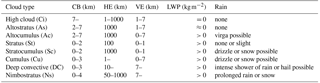
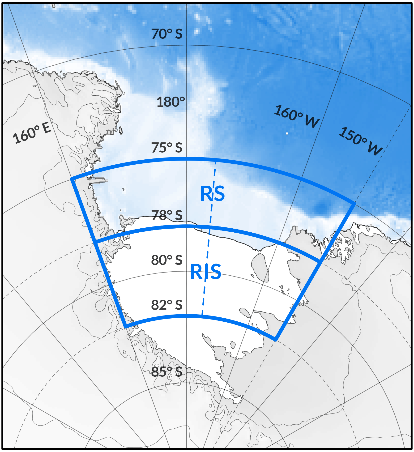
Figure 1Topographic map of the RIS and Ross Sea including the boundaries of the study area (thick blue line) and border between the RIS and Ross Sea sectors. (Map derived from the SCAR Antarctic Digital Database.)

Download

The area of interest in this study covers as much of the RIS as possible and extends into the southern Ross Sea. Defined by the edges of the ice shelf (160 to −150^∘ E), it extends from the bottom of the A-Train track at 82^∘ S north to 75^∘ S. The area is divided into two sectors (RIS and the Ross Sea) along the 78^∘ S circle of latitude, each of which are further divided into east/west sectors to form four quadrants. Figure 1 identifies the study region and its bounds. Note that despite the larger area of the Ross Sea compared to the RIS defined in this study, the number of vertical profiles linked to the RIS region is far higher than that for the Ross Sea (4.1 vs. 1.8 million). This disparity is associated with a strong latitudinal variation in the sampling density associated with the satellite orbits. This study uses observations made between 1 January 2007 and 31 December 2010 when both the CloudSat and CALIPSO satellites were fully operational and aligned.

In Sect. 3 we inspect cloud occurrence as a function of altitude for different cloud phases and the cloud fraction. The cloud occurrence is derived by counting the occurrence of cloud at a particular altitude using the CloudLayerBase and CloudLayerTop fields of the 2BCL4 product. This is in contrast to the methodology used in Verlinden et al. (2011), which used a threshold of 50 % for the CloudFraction field (fraction of lidar volumes in a radar resolution volume that contains hydrometeors) for determination of cloud occurrence. In this study we calculate the cloud fraction (not related to the CloudFraction field) as the complement of the clear sky fraction, which is the number of clear sky profiles divided by the total number of profiles. As such, it is independent of altitude.

2.2 Synoptic climatology

To provide context on atmospheric circulation over the duration of this study, classifications and regimes developed in the work of Coggins et al. (2014) and Coggins and McDonald (2015) are used. Five broad synoptic-scale regimes, hereafter referred to as “Coggins regimes”, encompass 20 classes created by applying the k means clustering technique to 10 m winds from 33 years of ERA-Interim reanalysis (Dee et al., 2011) over the RIS/Ross Sea region. The 20 classes grouped into five regimes were found to be representative of conditions in the area and span the entire time period of available cloud observations, and so are an obvious choice for this analysis. The first two Coggins regimes are the weak northern cyclonic (WNC) and strong northern cyclonic (SNC) regimes which feature cyclones to the north of the RIS, with the “weak” and “strong” ratings referring to their effect on the winds over the RIS; WNC generally provides weak forcing and low wind speeds, while SNC features a strong synoptic pressure gradient force and high wind speeds over the RIS. The Ross Ice Shelf airstream (RAS) Coggins regime covers the strongest winds over the RIS and typically features a strong cyclone to the north and east that provides a large pressure gradient over the ice shelf which forms RAS-like signatures (Parish et al., 2006), while the weak southern cyclonic (WSC) regime is associated with relatively weak cyclones and mesocyclones positioned over the RIS with medium wind speeds. Finally, the weak synoptic (WS) Coggins regime covers periods where a very weak pressure gradient and very low winds are present over the RIS.

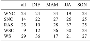
Table 2 shows the relative frequency of occurrence of the regimes over the entire observational period examined and a normalized seasonal frequency. Examination of the “all” column shows that the WSC regime is relatively rare (9 % annual frequency), while the WS regime is observed frequently (29 %). The WNC and RAS regimes are also quite common (25 and 23 % respectively), while SNC is less common (14 %). Seasonal analysis of the frequency of occurrence shows the WNC regime occurs most frequently during austral autumn (34 %) but much less frequently during winter (19 %), while the SNC regime is more uniform across all four seasons – this likely reflects the ubiquitous nature of synoptic-scale cyclonic storms around Antarctica (Hoskins and Hodges, 2005). The RAS regime is seen much more frequently in winter (37 %) than summer (10 %), while the WSC and WS regimes alternately favour autumn (WSC 36 %) and summer (WS 36 %) at the expense of summer (WSC 12 %) and autumn (WS 17 %). It must be noted that Table 2 is structured for seasonal analysis of individual regimes (rows sum to 100 %) and does not provide a comparable statistic of regime frequency in each season (season columns do not sum to 100 %).

Table 2Relative frequency of occurrence of the Coggins regimes annually (all) and seasonally (DJF–SON) in the ERA-Interim reanalysis (%). DJF/MAM/JJA/SON correspond to austral summer/autumn/winter/spring respectively. Values for seasons are normalized so that rows sum to 100 % (not including “all”).

Download Print Version | Download XLSX

3.1 Discontinuity in the 2B-GEOPROF-LIDAR R04 product

As an initial point of comparison with the previous Antarctic-wide studies of Verlinden et al. (2011) and Adhikari et al. (2012) we display seasonal mean cloud occurrence statistics in Fig. 2 derived from the 2BGL4, 2BGL5 and 2BCL4 products for the Ross Sea and the RIS. A visual comparison between the three products generally shows good agreement (within a few percentage points), though the 2BGL4 values of cloud occurrence are a little above the values derived from the other two products everywhere below 8 km. A step change in the cloud occurrence can also be observed at 8.2 km in all seasons and over both the Ross Sea and the RIS in the 2BGL4 product. It should be noted that this step change is particularly large in the winter and spring and is also significantly larger over the RIS than the Ross Sea. The 2BGL5 and 2BCL4 values do not display this discontinuity and are much more similar to each other, though it is noticeable that the 2BCL4 values of cloud occurrence are always smaller than the other two products below 1 km. Interestingly the temporal average cloud occurrence for the 2BGL4 product is always larger than that for the 2BCL4 product, which in turn is always greater than the 2BGL5 product.

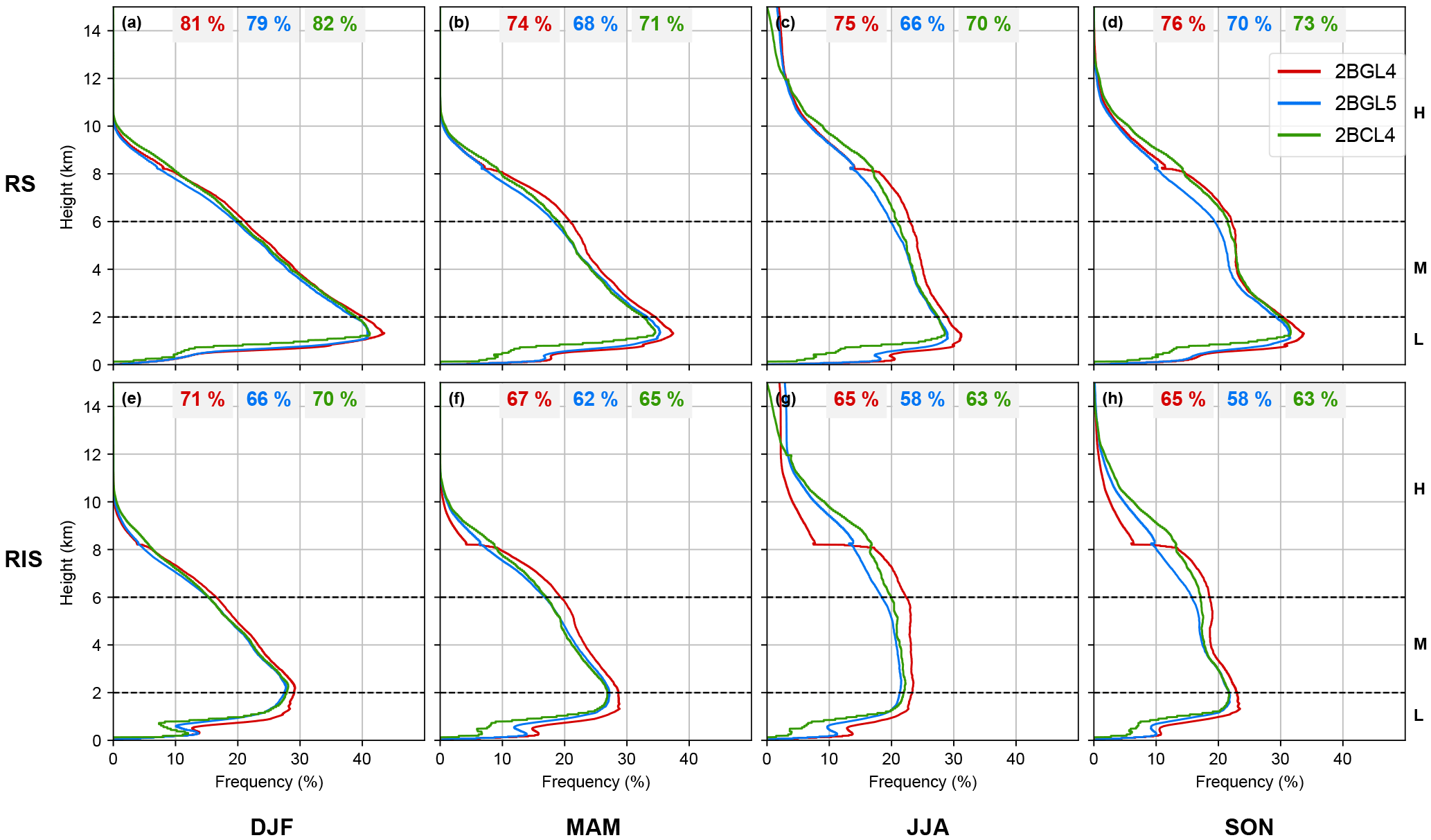
Figure 2Mean vertical profiles of cloud occurrence derived from the 2BGL4, 2BGL5 and 2BCL4 data for the Ross Sea (a–d) and RIS sectors (e–h) for different seasons. Total sector cloud fraction (temporal average cloud occurrence independent of altitude) is annotated at the top of each sub-figure. L, M, and H labels indicate the low, medium, and high cloud regions, respectively, as discussed in the text.

Download

To further examine the extent of this issue, Fig. 3 displays the zonal mean value of the ratio of the cloud occurrence at 8.3 km to the cloud occurrence at 8.0 km derived from the three products. The two altitude bins are in consecutive height bins, but are linked to different vertical and horizontal resolutions in the 2BGL4 processing scheme according to Mace et al. (2009). Inspection of Fig. 3 shows that the ratio varies between 0.9 and 1.1 for all three products near the Equator and at mid-latitudes. However, the 2BGL4 value of the ratio deviates significantly from that derived from the other two products at latitudes poleward of 75^∘ in both hemispheres. The deviation between the 2BGL5 product and the 2BCL4 product is also relatively large in the Northern Hemisphere above 60^∘ N. Previous studies (Adhikari et al., 2012; Bromwich et al., 2012; Verlinden et al., 2011) have highlighted this discontinuity near 8 km, but have questioned whether it is an instrumental artefact or a physical feature. The analysis in Fig. 3 clearly suggests that this is an instrumental artefact specific to both polar regions. The larger discontinuity observed in Fig. 2 in winter may suggest a temperature-dependent issue. But, further analysis is beyond the scope of this study given the good correspondence between the 2BCL4 and 2BGL5 products.

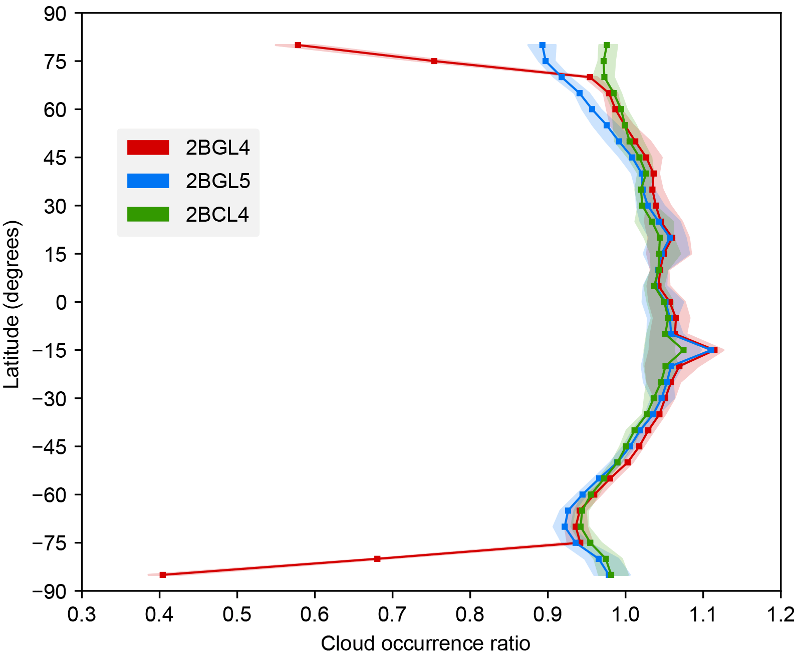
Figure 3Latitudinal variation of the ratio of cloud occurrence at 8.3 km to cloud occurrence at 8.0 km derived from the 2B-GEOPROF-LIDAR products and the 2B-CLDCLASS-LIDAR products. The envelopes represent the interquartile ranges of the ratio observed at that latitude. Note that consistently anomalous values ≪1 are confined to the polar latitudes.

Download

3.2 Cloud occurrence and phase by season

Given the uncertainty identified within the 2BGL4 (GEOPROF) product, we choose to deviate from previous studies and use the 2BCL4 (CLD-CLASS) product. We consider this preferable to the 2BGL5 product, despite the apparent resolution of the uncertainties in 2BGL4, as it provides information on cloud phase and type, which are particularly interesting in this region. We initially examine cloud occurrence as a function of cloud phase. Adhikari et al. (2012) reported that the largest seasonal variations in cloud occurrence were observed over the RIS and sea ice region in the surrounding Ross Sea, suggesting this region may be of particular interest in understanding the controls of cloud in the region. Cloud occurrence is separated into two sectors: the Ross Sea and the RIS (see Fig. 1). For the purpose of this analysis we separate clouds into three vertical ranges: low-level clouds (0–2 km), mid-level clouds (2–6 km) and high-level clouds (6– km) identified by horizontal lines in Figs. 2, 4 and 5.

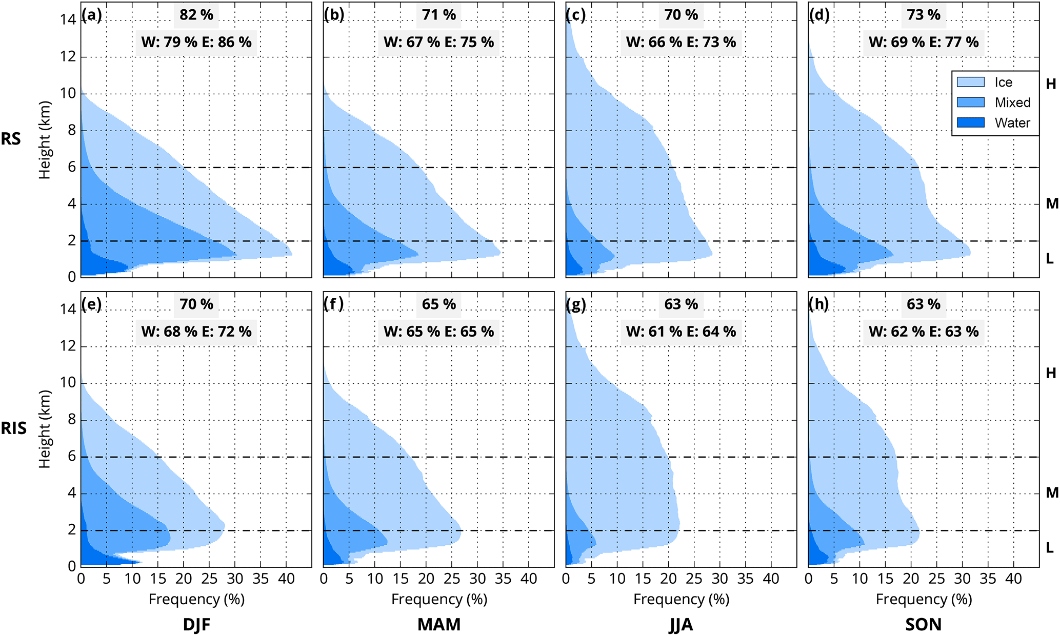
Figure 4Mean vertical profiles of cumulative cloud occurrence for different cloud phases derived from 2BCL4 data for the Ross Sea (a–d) and RIS sectors (e–h) for different seasons. Total sector cloud fraction (temporal average cloud occurrence independent of altitude) is annotated at the top of each sub-figure, along with values for the western (W) and eastern (E) halves of each sector. L, M, and H labels indicate the low, medium, and high cloud regions, respectively, as discussed in the text.

Download

Figure 4a–d display the cloud occurrence for the Ross Sea region in each season broken into different cloud phases (shaded areas). The maximum cloud fraction (82 %) is observed during summer, with the minimum cloud fraction (70 %) observed during winter. The largest cloud fraction is observed over the eastern portion of the Ross Sea in every season, with the greatest seasonal cloud fraction in summer (86 %). The smallest cloud fraction (66 %) was observed in winter over the western portion of the Ross Sea. Cloud occurrence as a function of altitude shows the same pattern, with the maximum (about 40 %) occurring in summer and the minimum (about 27 %) during winter. Though all maxima occur between 1.5 and 2 km above sea level (a.s.l.), the winter maximum is noticeably weaker. Mixed phase clouds are predominant near the cloud occurrence altitudinal maximum, with water and ice cloud contributing roughly equally to the remainder. Changes in the occurrence of mixed phase cloud appear to constitute the majority of the change in the cloud occurrence at that altitude.

Cloud occurrence reduces uniformly at increasing altitude from the maxima in summer and autumn, while in winter the cloud occurrence reduces rapidly between the peak and 3.5 $\mathrm{km}\mathrm{a}.\mathrm{s}.\mathrm{l}.$, and then remains relatively uniform before a more rapid reduction at higher altitudes (8 km in winter and 6 km in spring). Previous work detailed in Verlinden et al. (2011) highlighted a discontinuity in cloudiness near 8 $\mathrm{km}\mathrm{a}.\mathrm{s}.\mathrm{l}.$ over much of the continent which appears to be linked to the processing artefact identified previously.

Unlike the study of Verlinden et al. (2011) we do not observe two distinct maxima in the vertical profiles of the cloud occurrence; however, this feature was relatively weak over the WAIS (Verlinden et al., 2011), which may hint at the specific drivers of the cloud environment in this region. In particular, the absence of a secondary peak in mid- and high-level cloud occurrence is interesting given the ubiquitous nature of cyclones in the region (Hoskins and Hodges, 2005), and the muted seasonal signal in cloud occurrence above 2 $\mathrm{km}\mathrm{a}.\mathrm{s}.\mathrm{l}.$ could be explained by the lack of a strong seasonal signal in cyclone frequency in this region (supported by the small seasonal signal in the frequency of the SNC regime displayed in Table 2). The difference in our cloud occurrence calculation methodology to that used by Verlinden et al. (2011) may have some impact; however, it is unlikely to explain all of the difference.

As might be expected, the liquid water phase occurs predominantly in low-level clouds with a local maximum between 300 and 900 $\mathrm{m}\mathrm{a}.\mathrm{s}.\mathrm{l}.$ in all seasons, the largest enhancement occurring during summer. The difficulty of detecting cloud within 1 km of the ground using CloudSat due to ground clutter (Haynes et al., 2011; Mace et al., 2009) may bias low-level cloud detection in favour of periods of reduced attenuation of the CALIOP lidar instrument (clear sky or optically thin mid- to high-level cloud). Mid-level (between 2 and 6 $\mathrm{km}\mathrm{a}.\mathrm{s}.\mathrm{l}.$) cloud occurrence varies little between seasons at the upper limit (6 km) at close to 20 %, but mid-level cloud fraction is greatest in summer and lowest in winter. More high-level cloud (above 8 $\mathrm{km}\mathrm{a}.\mathrm{s}.\mathrm{l}.$) is observed during winter than summer, which matches with the results identified in Adhikari et al. (2012). We also note that clouds were not observed in this study above 10 $\mathrm{km}\mathrm{a}.\mathrm{s}.\mathrm{l}.$ in both the summer and autumn, or 12 km in spring, but were seen above 14 km in the winter. Haynes et al. (2011) suggest that the maximum cloud height over the Southern Ocean will be impacted by the seasonal variations in tropopause depth likely explains this pattern, which interestingly shows a similar seasonal progression to that for polar stratospheric cloud occurrence (Alexander et al., 2011, 2013).

The mean seasonal cloud occurrence vertical profiles for the RIS are displayed in Fig. 4e–h. The eastern portion of the RIS has slightly greater cloud occurrence than the western portion of the RIS in all seasons apart from autumn. The cloud fraction for the RIS area is 70 % in summer and between 63 and 65 % in all other seasons. The greatest cloud fraction by sector is observed over the eastern RIS during summer (72 %), while the lowest is observed in winter over the western RIS (61 %). Inspection of the cloud occurrence as a function of altitude shows a maximum at approximately 2 $\mathrm{km}\mathrm{a}.\mathrm{s}.\mathrm{l}.$ in every season, slightly higher than the altitude of the peak observed over the Ross Sea. This peak in cloud occurrence matches with a similar peak in ice water content (IWC) and liquid water content (LWC) values discussed in Scott and Lubin (2016) over Ross Island (located at the south-western corner of the Ross Sea region in this study). Summer experiences the greatest cloud occurrence as a function of altitude at this peak, but the seasonal variability is rather muted (just under 5 % variation across all seasons) relative to that observed over the Ross Sea (approximately 12 %), with the minimum in winter. The mixed phase class is a contributor to this peak in all seasons, but is dominant in summer. The cloud occurrence linked to the ice phase is slightly larger than that for mixed phase cloud in autumn.

Again, the water phase occurs predominantly for low-level clouds (below 2 $\mathrm{km}\mathrm{a}.\mathrm{s}.\mathrm{l}.$) with maxima below 600 m observed in every season (this is particularly clear for summer). The ice phase is effectively the only contributor for high-level clouds (above 6 km) and is the largest contributor to cloud occurrence in every season, though mixed phase cloud is dominant up to approximately 3 km in summer. The quantity of mixed and water phase cloud as a proportion of total cloud occurrence is substantially lower than that observed over the Ross Sea, possibly suggesting a lack of moisture in this region and the impact of colder temperatures.

The seasonal variation in cloud occurrence at mid-levels (between 2 and 6 $\mathrm{km}\mathrm{a}.\mathrm{s}.\mathrm{l}.$) is approximately 5–10 %, which is smaller than the variations observed at the peak occurrence level. Within this altitude range, cloud occurrence is more constant in winter and spring and reduces with altitude in spring and summer. The cumulative occurrence of mid-level clouds is marginally higher in summer than other seasons, with a minimum value in winter. High-level clouds (above 6 km) are distinctly more common in autumn and winter than spring and summer. Similar to the Ross Sea case, the majority of clouds are limited to below 10 $\mathrm{km}\mathrm{a}.\mathrm{s}.\mathrm{l}.$ in both the summer and autumn, with maximum high-cloud occurrence in winter. Over the entire vertical profile, the seasonal variation over the RIS is smaller than that observed over the Ross Sea (cf. Fig. 4a–d and e–h).

3.3 Cloud occurrence and phase by synoptic regime

We now examine composites of the vertical distribution of cloud occurrence and cloud fraction for these two regions based on the synoptic-scale Coggins regimes. Figure 5a–e display the cloud occurrence profiles over the Ross Sea for the five different Coggins regimes. Comparison of Fig. 5a–e shows that the combined cloud occurrence (associated with the three different cloud phase classes) in every regime again maximizes just below 2 $\mathrm{km}\mathrm{a}.\mathrm{s}.\mathrm{l}.$ The greatest occurrence at that peak is observed in the SNC regime and the smallest occurrence in the WSC regime. At middle altitudes (4 to 6 km), the difference in cloud occurrence between regimes is very large, with the SNC regime again displaying the largest cloud occurrences (between 28 and 35 % in this altitude range) and the WSC regime the least (between 7 and 17 %). The WSC and WS regimes have rather similar vertical profiles, with the vast majority of cloud occurrence linked to low- to mid-level clouds below 4 $\mathrm{km}\mathrm{a}.\mathrm{s}.\mathrm{l}.$ The SNC type on the other hand has high cloud occurrence at nearly all levels compared to the other regimes and has signs of a secondary maximum at 5 km. The RAS and WNC have intermediate levels of cloud occurrence between the SNC and WSC/WS regimes, with shallower rates of reduction in the cloud occurrence above the peak.

Inspection of the distribution of phases linked to the SNC regime (linked to strong cyclonic activity in the north of the Ross Sea) suggests that this regime is dominated by ice cloud at all levels down to about 2 $\mathrm{km}\mathrm{a}.\mathrm{s}.\mathrm{l}.$ (i.e. mid- to high-level clouds are predominately comprised of ice). A small amount of water phase cloud is observed very close to the surface and a peak in mixed phase cloud is observed just below the peak in the combined cloud occurrence. The quantity of mixed phase cloud being larger than the ice phase only occurs in the WS and WNC types near the low-level maxima. The SNC and RAS regimes feature the largest proportion of ice cloud overall. The cloud fraction (see labels in Fig. 5) varies from 82 % for the SNC regime to 58 % for the WSC regime, with the other regimes having values between 72 and 77 %. This variation is significantly larger than that observed when observations are composited based on season. This result suggests that cloud fraction is strongly impacted by synoptic situation. In particular, the SNC regime has high occurrence frequencies in the mid- to high-level cloud region above 2 $\mathrm{km}\mathrm{a}.\mathrm{s}.\mathrm{l}.$ Additionally, we note that the variation between the western and eastern portions of the Ross Sea is larger in the SNC, RAS, and WSC regimes (10–13 %) than over the seasons (7–8 %), while the WNC regime shows little variation longitudinally. This suggests that synoptic forcing is a more important control on longitudinal differences than season, though this should be expected because the strength and position of cyclonic centres is a principal determinant of the Coggins regimes. While overall the synoptic typing seems to be important, we note that the proportion of liquid and mixed phase cloud varies relatively little over the Ross Sea as a function of the Coggins regimes (between approximately 15 and 20 % at the altitude of maximum occurrence), while the seasonal variation is substantially larger (between approximately 9 and 30 % at the altitude of maximum occurrence). This result supports the view that temperature is a strong driver of the occurrence of ice cloud as previously identified by Haynes et al. (2011), though the variability observed between synoptic types suggests that temperature anomalies associated with specific synoptic types also have some influence.

Figure 5f–j display composites for the RIS for the Coggins regimes. Cloud occurrence is significantly smaller in every regime relative to the profiles over the Ross Sea (cf. Fig. 5a–e). Examination of the cloud occurrence profiles as a function of altitude for each regime suggests that the WNC, WSC, and WS regimes have similar forms, as do the SNC and RAS regimes (to each other). Interestingly, cloud occurrence is higher in the RAS regime between 2 and 6 km than SNC. This likely suggests that the impact of cyclones in the northern Ross Sea is not as strong an influence on cloud over the RIS. At mid to high levels (above 4 km), RAS and the SNC have the largest cloud occurrences, with ice cloud dominating in this region. The variation at upper levels is also noticeably larger between the various synoptic regimes in Fig. 5 than between the seasons displayed in Fig. 4. This seems to suggest that the synoptic state is a stronger driver of mid- to high-level cloud than seasonal variations, this being particularly clear when we consider that the regime with most high-level cloud (the SNC regime) displays almost no seasonality (see Table 2). Figure 5 therefore shows an advantage in using a classification scheme based on synoptic states relative to one using seasons in this region. Previous work by Haynes et al. (2011) also suggested that seasonality might not be a strong influence on the Southern Ocean, with two exceptions, these being the quantity of ice cloud and the height at which the maximum cloud fraction occurs in the upper troposphere.

Examination of the cloud fraction over the entire RIS and the western and eastern sectors shows less variability than over the Ross Sea. The cloud fraction varies only between 55 and 68 % and the differences in cloud fraction between the western and eastern sectors are only sizeable (9 %) for the WSC regime. The difference between the cloud fraction between the western and eastern sectors is 5 % or less in all other regimes. Given that the WNC and SNC regimes are dominated by the positions of cyclones over the Ross Sea, this may not be surprising in those cases. However, the lack of longitudinal variation associated with the RAS which is traditionally linked to flow near the TAM is a surprise.

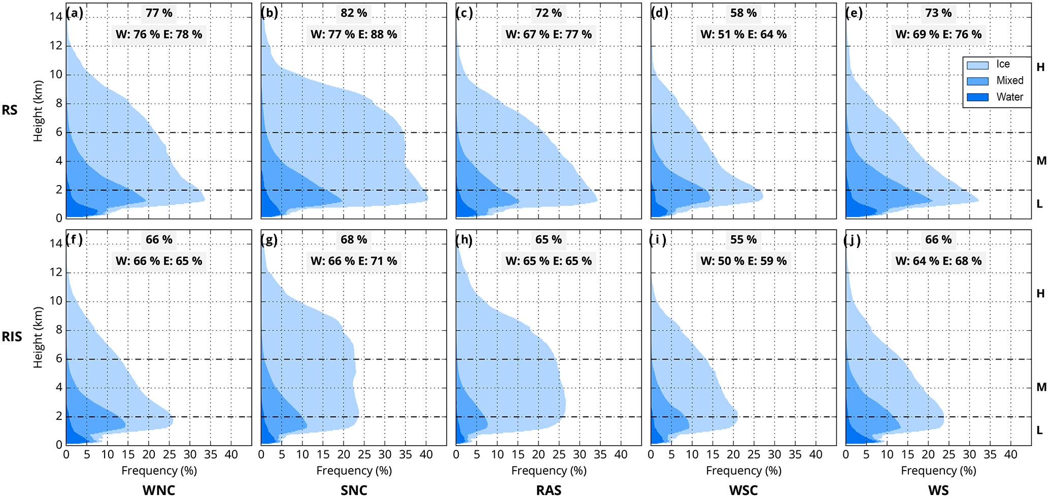
Figure 5Mean vertical profiles of cumulative cloud occurrence for different cloud phases derived from 2BCL4 data for the Ross Sea (a–e) and RIS regions (f–j) for the Coggins regimes. L, M, and H labels indicate the low, medium, and high cloud regions, respectively, as discussed in the text.

Download

3.4 Multilayer cloud by season and regime

While useful, the mean vertical profiles of cloud occurrence displayed in Figs. 4 and 5 do not fully represent the individual profiles composited in that season or regime. For example, two states associated with a distinct high and low cloud type might be combined in the averaging process to form the mean cloud occurrence observed. Alternatively, multi-layered cloud might be present and contribute to the mean cloud occurrence profiles. In an effort to display this variability, Fig. 6 shows the quantity of clear skies, single-layer cloud, and multi-layer cloud for the Coggins regimes and seasons over the Ross Sea and RIS. Inspection of Fig. 6a for the Ross Sea region suggests that clear skies are observed 26 % of the time on average. However, when the cloud occurrence information is composited based on the Coggins regime, the frequency of occurrence of clear skies varies between 18 % for the SNC regime and 42 % for the WSC regime. Seasonal variations in clear sky occurrence are considerably smaller at 18 to 30 %. Again, this highlights that clouds are observed preferentially in the Ross Sea when strong cyclonic centres are observed in the northern Ross Sea. Changes in the frequency of multi-layer clouds are also notable, with the frequency varying from 15 % for the WSC regime to 33 % for the SNC regime. The occurrence of multi-layer cloud is considerably more constant as a function of season, varying between 21 and 25 %, which highlights that the quantity of multi-layer cloud is also strongly impacted by synoptic conditions.

Figure 6b displays the occurrence of clear skies, single-layer cloud and multi-layer cloud for the RIS region. The variability as a function of both Coggins regime and season is again muted relative to the Ross Sea region. The occurrence of clear skies varies from 32 % for the SNC regime to 45 % for WSC, with the other three regimes having frequencies between 34 and 35 %, which is similar to that for the SNC regime. This suggests that only the synoptic conditions linked to the WSC regime are strongly linked to clear skies. When clear sky occurrence is examined as a function of season, a very small seasonal variability is observed (values fall between 30 and 37 %). This reinforces our previous conclusion for the Ross Sea region: that clear skies are not strongly influenced by season and therefore surface temperatures. Examination of multi-layer cloud values shows a variation between 15 % for WSC and 23 % for both the RAS and SNC types. This suggests that the RAS regime is also preferentially related to multi-layer cloud over the RIS. Work by Steinhoff et al. (2009) has previously suggested that the RAS regime might be linked to the occurrence of low- and mid-level cloud, the latter being associated with vertical ascent generated by low-level convergence as the RAS decelerates downstream of wind speed maximum along the TAM. This relationship also appears to be observed based on our statistical analysis. The high occurrence of cloud at mid-levels (between 2 and 6 $\mathrm{km}\mathrm{a}.\mathrm{s}.\mathrm{l}.$) displayed in Fig. 2g therefore suggests that the RAS and possibly the marine air intrusions identified in Nicolas and Bromwich (2011) have a noticeable climatological impact on cloud occurrence over the RIS. In addition, the seasonal progression and variation linked to synoptic typing display very different impacts over the Ross Sea and RIS. This perhaps highlights the stronger influence of cyclones on cloud occurrence over the Ross Sea than the RIS. The higher frequency of occurrence of multi-layer cloud linked to the SNC type over the Ross Sea than the RIS also suggests the position of the cyclone centre plays an important role in cloud distributions.

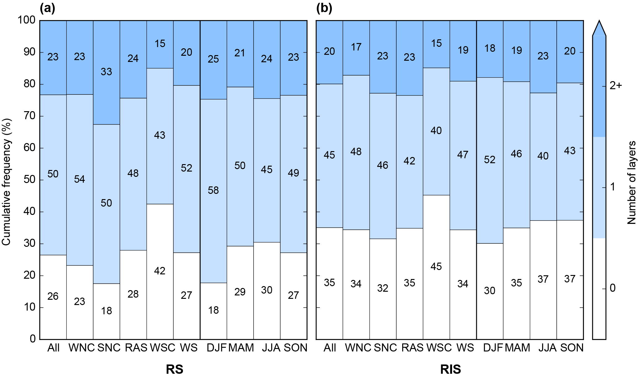
Figure 6Distribution of the number of cloud layers over the Ross Sea and RIS for all cases, the Coggins regimes and season.

Download

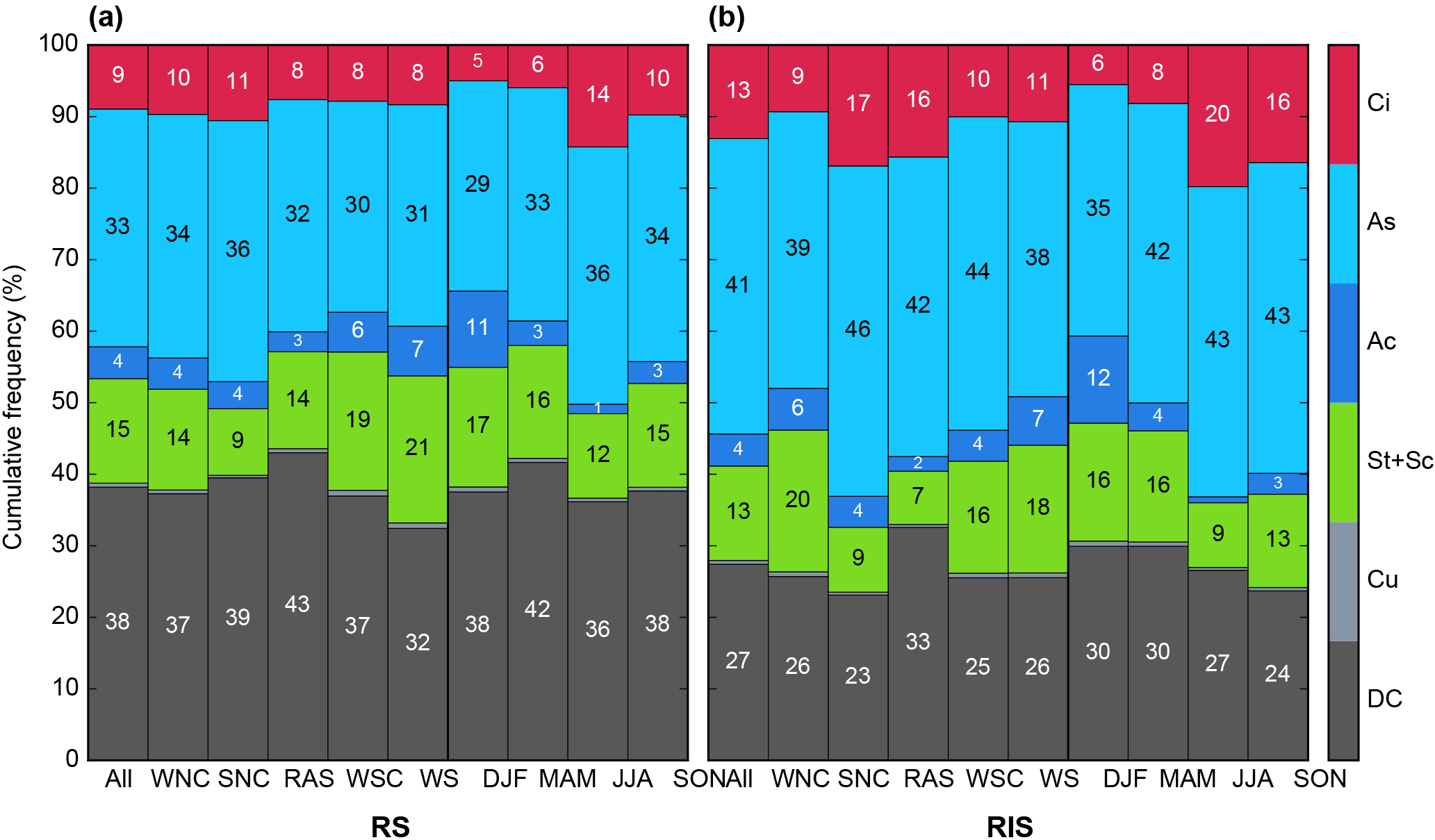
3.5 Cloud type by season and regime

Figure 7 displays the fractional occurrence of the various cloud types over the Ross Sea and RIS composited based on Coggins regime and season. For the sake of conciseness, we will only discuss the types which have substantial fractional occurrence rates (above 15 % in any class). The frequency of nimbostratus (Nb) is so small over these regions that this type is not included in Fig. 7. For the Ross Sea, the most commonly occurring cloud type is deep convective (DC), which varies from 32 % for the WS regime to 43 % for the RAS regime, with the other regimes ranging between 32 and 39 % (see Fig. 6a). This cloud type is likely identified due to large horizontal and vertical extents of the cloud rather than the presence of deep convection in the polar region. The seasonal variation has a maximum in autumn of 42 % with a minimum of 36 % in winter. Thus, in this high-level cloud type, more variation between classes is associated with synoptic classification than season. Interestingly the maximum occurrence of this type over the Ross Sea is associated with the RAS regime rather than the SNC regime, previously identified as the regime associated with the highest cloud occurrence. When we additionally include the impact of clear skies (values displayed in Fig. 6), this conclusion remains unchanged.

The next most common cloud type over the Ross Sea is the altostratus (As) type, which varies between 30 and 36 % based on Coggins regimes and between 29 and 36 % based on season. In particular, the fractional occurrence of this cloud type maximizes in winter and minimizes in summer over the Ross Sea. However, when the frequency of clear skies (see Fig. 6) is also considered, the seasonal variation becomes very small (23 to 25 %), while the regime variation is enhanced to 17 to 30 %. Thus, in this case close inspection also suggests that synoptic forcing is a driver of the occurrence of this cloud type, with the highest occurrence in the SNC regime and lowest occurrence in the WSC regime. Note that the As type is predominantly a mid- to high-level cloud dominated by ice and thus may not be strongly impacted by seasonally varying quantities, such as sea ice cover and surface temperature.

Low-level clouds (combined stratus/stratocumulus or St∕Sc types) are observed relatively frequently in the WS (21 %) and WSC (19 %) regimes over the Ross Sea. Both these regimes are associated with weaker synoptic forcing and observed less frequently than the regimes with stronger synoptic forcing. Seasonal variation in these types changes from 17 % in summer to 12 % in winter. Thus, it seems that the occurrence of this class is more associated with periods of weak synoptic forcing; note that these conditions occur more often in summer (see Table 2), which in turn might suggest that local factors are important. Inclusion of information on clear sky rates does not change this result.

Figure 7b displays cloud type fractional frequency information for the RIS region. Over the RIS, the As cloud type is most prevalent, varying between 38 and 46 % based on synoptic regime and 25 and 43 % based on season. However, when clear sky occurrence is considered these values reduce to 24 to 32 % for the regimes and 25 to 27 % for the seasons. This suggests that the quantity of altostratus remains nearly constant seasonally. The highest occurrence of the As type when clear skies are taken into consideration is linked to the SNC and RAS regimes, with very similar low occurrences (24 to 25 %) for the other regimes.

The next most prevalent cloud type over the RIS is the DC type, which changes between occurrence rates of 23 and 33 % for the various Coggins regimes and 24 and 30 % based on seasons. The highest fractional occurrence of the DC type occurs for the RAS regime and the minimum is, surprisingly, linked to the SNC type. Thus, two regimes which are related to strong synoptic forcing in the region have very different impacts on this cloud type. This latter result might be explained by the position of the cyclonic centres, preferentially in the north-eastern Ross Sea for the SNC type, relative to the RIS. When the frequency of clear skies is included in our analysis, a larger variation in this cloud type is linked to synoptic forcing than seasonal changes.

The combined St and Sc cloud types also have an appreciable occurrence rate over the RIS (13 %). When the Coggins regimes are considered this type has a minimum occurrence of 7 % linked to the RAS regime and a maximum occurrence of 20 % linked to the WNC regime. It should be noted that there is an obvious change in the fractional frequency of this type between strong synoptic forcing regimes (RAS and SNC) and weaker synoptic forcing regimes (WNC, WSC, and WS). This separation again suggests that these clouds are linked to periods of weak synoptic forcing. The range of the fractional occurrence rates associated with the different seasons is again smaller than that associated with the synoptic types; summer displays the highest occurrence rate. When clear sky frequencies are included in calculations this result is unchanged.

The fraction of the cirrus (Ci) cloud type is also appreciable over the RIS and has the same frequency of fractional occurrence as the combined St and Sc cloud type (13 %). The fraction of this cloud type maximizes at 17 % for the SNC regime and has a minimum occurrence of 9 % for the WNC regime. The Ci type is observed most frequently in winter (20 %) and least in summer (6 %). Thus, synoptic variations do not appear to be a very strong control on this cloud type. This conclusion is unchanged when the occurrence of clear skies is included in our analysis. We note that the larger fractional occurrence of Ci over the RIS compared to the Ross Sea could be associated with the proximity of the TAM to the RIS and the influence of isolated cirrus generated by orographically forced waves, this conjecture being supported by Haynes et al. (2011) and Scott and Lubin (2016).

Figure 7Percent fraction of cloud types over the Ross Sea and RIS for all cases, the Coggins regimes and seasons. The cloud types are identified in Table 1.

Download

3.6 Cloud height and thickness

Figure 8a and f display joint histograms of the cloud top height vs. the geometric cloud thickness over the Ross Sea and RIS respectively. Figure 8a shows that low-level (below 2 $\mathrm{km}\mathrm{a}.\mathrm{s}.\mathrm{l}.$) thin cloud (thicknesses below 3 km) has a high occurrence over the Ross Sea, an observation previously identified by Adhikari et al. (2012). However, thin clouds are observed relatively frequently for cloud top heights between the surface and approximately 8 km over the Ross Sea. Clouds that effectively cover nearly the complete vertical column to cloud top (i.e. that have similar thicknesses to their cloud top height) are also observed frequently. We also note that clouds with high cloud tops (above 6 km) are relatively rare. The logarithmic scale associated with Fig. 8 highlights that thin low-level cloud is very common. A similar pattern is observed over the RIS region overall (see Fig. 8f), though cloud occurrence is higher in general for the Ross Sea, particularly at lower levels. This is to be expected, given the differences in solar heating of the surface, sea ice concentration changes and sea surface temperatures. In particular, the greater availability of moisture over the Ross Sea associated with open water in summer would likely be an important contributor. The overall pattern is similar to the joint histograms identified by Haynes et al. (2011) over the Southern Ocean.

To further understand the distribution of clouds over the two regions, Fig. 8b–e and g–j display anomalies from the annual means for each season for the Ross Sea and RIS respectively. Examination of Fig. 8b–e suggests that the anomaly patterns are rather similar in the summer and autumn, with higher cloud occurrence observed for low-level (below 2 km) and mid-level (2 to 6 km) cloud which covers the majority of the vertical column up to the cloud top height. Lower cloud occurrence is associated with thin high top clouds for summer and autumn. The anomaly patterns in winter and spring are near mirror images of those in summer and autumn, with higher cloud occurrence for thin high top cloud and lower occurrence (relative to the annual mean) for low-level and mid-level cloud covering the vertical column. High top clouds (above 8 km) with a range of thicknesses are also enhanced in winter and spring, with the enhancement being more noticeable for thick clouds in winter. Haynes et al. (2011) previously identified that the increase in thicker clouds in winter over the Southern Ocean may be associated with storm track activity. Haynes et al. (2011) also suggest that the maximum cloud height might vary seasonally based on the tropopause height; therefore, this also seems like a reasonable explanation for the enhanced occurrence of high-level cloud above 8 km in the winter relative to the summer. The anomaly patterns for each season are generally rather similar over the Ross Sea and the RIS. This is surprising since this may imply that moisture availability is not a large driver of cloud.

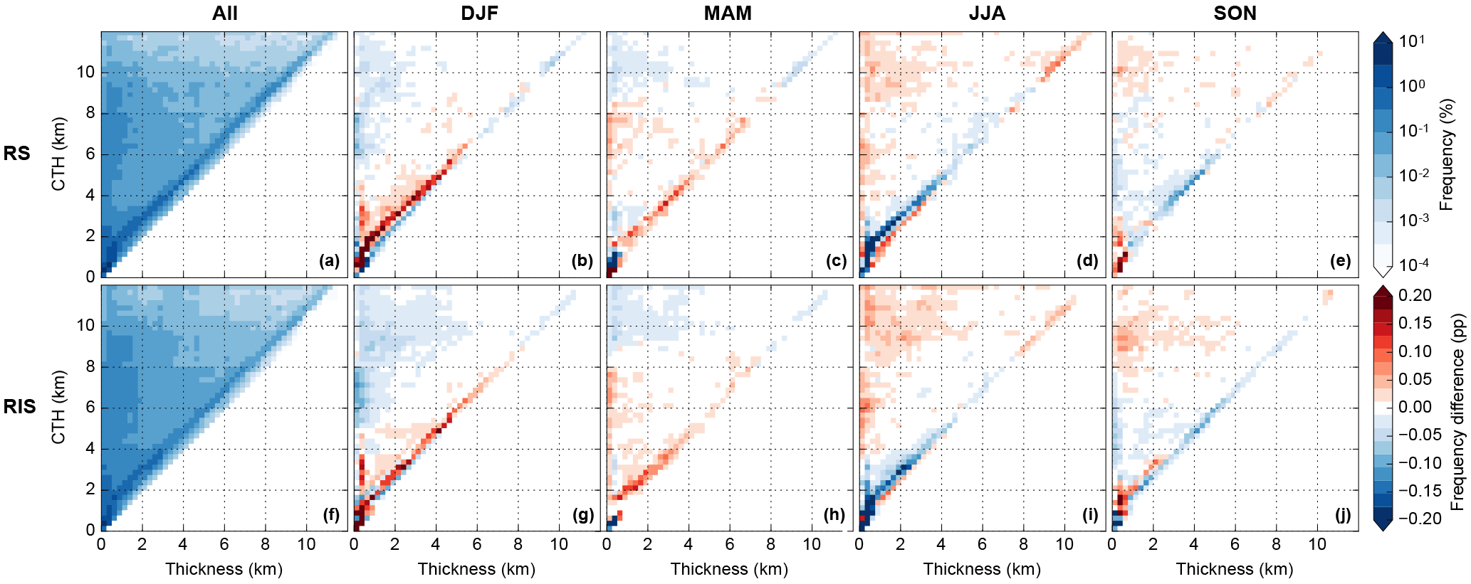
Figure 8Joint histogram of the cloud top height vs. geometric cloud thickness over the Ross Sea and RIS for the entire year on a logarithmic scale (a, f) and the difference from the annual mean over the respective region (RS and RIS) for each season on a linear scale (b–e, g–j).

Download

Figure 9b–f and h–l display the anomalies from the mean associated with the Coggins regimes for the Ross Sea and RIS respectively. Figure 9a and g display histograms of the frequency of occurrence as a function of thickness and cloud top height for the Ross Sea and RIS respectively, are exact reproductions of Fig. 8a and f and are included to aid in interpretation. Inspection of the anomalies from the mean linked to different synoptic regimes shows some interesting structures. The SNC regime is linked to a dearth of low-level cloud relative to the mean, particularly over the Ross Sea, while the WSC regime is linked to a considerable enhancement in the frequency of low- and mid-level cloud which covers the majority of the vertical column up to the cloud top height. These variations may also explain the small quantity of multi-layer cloud in this regime over the Ross Sea. The enhancement in the WSC regime is also observed in the WS regime, but that regime is also related to a stronger reduction in clouds covering the vertical column above 4 km. For the SNC regime, the dearth in low-level cloud over the Ross Sea is counter-balanced by an increase in thick (greater than 7 km deep) high-level cloud relative to the mean, which also accounts for the increased cumulative cloud occurrence for the SNC regime identified in Figs. 5b and 6a. While some aspects of the anomaly for the RAS regime (see Fig. 9d) are similar to the SNC regime pattern (see Fig. 9c), notably a reduction in low-level cloud relative to the mean, differences can be observed. For example, the clouds with high cloud tops (above 8 $\mathrm{km}\mathrm{a}.\mathrm{s}.\mathrm{l}.$) are under- rather than over-represented relative to the mean for the entire thickness range for RAS compared to SNC. Enhanced cloud occurrence in the RAS regime is primarily limited to mid-level clouds, most notably linked to clouds with thicknesses below 2 km and the region identifying that the cloud covers nearly the full atmospheric column.

To put the anomaly patterns identified for the Ross Sea into context, it is also worthwhile considering the patterns over the RIS (Fig. 9h–l). Unlike the seasonal analysis presented in Fig. 8, which displayed large similarities for the anomaly patterns over the Ross Sea and RIS, the patterns show more variability for the WNC, SNC, and RAS regimes between the two regions. In particular, the WNC regime displays a strong enhancement in the quantity of low- and mid-level cloud below 4 $\mathrm{km}\mathrm{a}.\mathrm{s}.\mathrm{l}.$, with thin cloud and cloud covering the majority of the atmospheric column up to the cloud top height being enhanced. The SNC type shows a similar pattern to that over the Ross Sea, but the strong enhancement of deep, high cloud top height cloud is not observed in this case. The RAS regime joint histogram shows a stronger reduction in low- and mid-level cloud below 4 km over the RIS than the Ross Sea and the enhanced cloud occurrence region now occurs for high-level cloud (cloud top height above 6 $\mathrm{km}\mathrm{a}.\mathrm{s}.\mathrm{l}.$). Thus, the vertical extent of the RAS regime changes considerably between the Ross Sea and the RIS. Based on previous work detailed in Steinhoff et al. (2009) this may be associated with vertical ascent over the RIS.

Figure 9Joint histogram of the cloud top height vs. geometric cloud thickness over the Ross Sea and RIS for the entire year on a logarithmic scale (a, f) and the difference from the annual mean over the respective region (RS and RIS) for each Coggins regime on a linear scale (b–e, g–j).

Download